Design and Implementation of a

Prognostic and Health Monitoring System

for the Power Electronics Converter

of a FEV Powertrain

DISSERTATION

submitted in partial fulfillment of the requirements for the degree of

Doctor of Philosophy in Applied Engineering by

Daniel Astigarraga Trespaderne

under the supervision of

Dra. Ainhoa Galarza Rodríguez

and

Dr. Luis Fontán Agorreta

Donostia – San Sebastián

July 2016

Acknowledgements

El trabajo contenido en el presente documento no se podría haber desarrollado sin la ayuda y el apoyo de muchas personas e instituciones, por lo cual, me gustaría agradecérselo de antemano.

Primeramente, me gustaría agradecer a TECNUN (Escuela de Ingenieros de la Universidad de Navarra) y a CEIT-IK4 la oportunidad que me brindaron al permitirme desarrollar el presente trabajo de investigación, por la confianza depositada en mí para el desarrollo de los proyectos en los que he estado envuelto y por poner a mi disposición todos los medios humanos y materiales. Asimismo, querría expresar mi gratitud al Departamento de Educación, Universidades e Investigación del Gobierno Vasco por el apoyo financiero a través del Programa Predoctoral de Formación de Personal Investigador (Beca: PRE_2014_2_200).

Estoy profundamente agradecido a mi directora, Ainhoa Galarza, por la confianza, la guía, y el ánimo otorgados en los buenos y en los malos momentos, así como por enseñarme la importancia de los detalles y el trabajo bien realizado. De la misma forma, me siento infinitamente endeudado con mis co-directores, Luis Fontán y Miguel Martínez-Iturralde. Por sus sabios consejos, por introducirme en la investigación y por depositar en mí su confianza para arrancar uno de los proyectos más bonitos en los que posiblemente trabaje. Gracias por vuestra entrega durante estos años, por dedicarme tiempo cuando no lo había y por el placer de trabajar con vosotros.

Debo agradecer a Joseba Echeverría y Joaquín de Nó, su apoyo y permitirme ser parte de la familia de TECNUN-CEIT en general, y de la División de Transporte y Energía en particular. No puedo olvidar a mi asesor académico durante los años de universidad, Francis Planes, y a la profesora Noemí Pérez por su ayuda, disponibilidad y simpatía. A pesar de llevarme alguna

ii Acknowledgements

reprimenda, gracias especialmente a Fernando Arizti por mostrarme parte de su sabiduría. Sin su ayuda este trabajo no habría sido posible.

Thanks to the HEMIS Project partners, especially to Beatriz, for your help and support. La ringrazio molto per il Dipartimento di Energia Nucleare presso il Politecnico di Milano per avermi accolto per tre mesi. Soprattutto gli Prof. P. Baraldi e Prof. E. Zio. Mi mancano i miei amici, “I tori di Bovisa”, Francesco, Matteo, Marco e Allegra. Chi vediamo presto.

Gracias a todos mis compañeros del laboratorio de Electrónica de Potencia en el presente, Ignacio, Federico, Ander, Fernando, Javi y en el pasado, Iker, Jorge, Jose Ángel, por hacer que cada día haya sido un placer ir a trabajar, así como por todo lo aprendido a vuestro lado. Aipamen berezia eman behar dizut, Ane Miren, zure laguntza irribarre batekin beti emateagatik. De la misma forma, gracias a todos con los que he compartido momentos entrañables de cenas y viajes, que espero sigamos organizando, Borja, Marco, Dámian, Gurutz, Goya, Aitor, Ainhoa, David.

Gracias a todos los alumnos que formáis el equipo del vehículo eléctrico, TECNUN SEED RACING, por hacer que cada día sea una nueva aventura y por luchar juntos para lograr los objetivos. De forma especial a Mikel, Beñat y Javi G., y a los alumni, Imanol, Lander, Peral, Álex, Edu, espero que continuéis cambiando el mundo con vuestra energía. Gracias José Macayo por tu disposición a enseñar y a ayudar siempre con una sonrisa, sin ti, muchos retos no habrían sido posibles. Gracias Manu Sánchez por las conversaciones agradables y por preocuparte de los demás antes que de ti mismo.

Por supuesto, no puedo olvidar a todos mis amigos fuera del entorno laboral. Empezando por los exalumnos de Tecnun, Ekain, Ibon, Jabi, Josu, Asier, Beñat, Jorge, Urko, Irene, Leire, Eider, Nerea, hemos disfrutado y lo seguiremos haciendo de buenos y divertidos momentos juntos.

Gracias a mis amigos y compañeros del Waterpolo Easo, Arizti, Gorka, Totti, Urtzi, Imanol, Santi, Jon, Iván, Ainara y en especial, Óscar, por ayudarme a mejorar cada día, por compartir tantos buenos momentos y por hacer que el esfuerzo merezca la pena.

Gracias a la kuadri, Unai, Diego, Iñaki, Julen, César, Iker, Jon, Iñigo, David, Potxo, Javi. Hace mucho que nos conocemos y sabéis lo importantes

Acknowledgements iii

que sois para mí. A pesar de no poder vernos tan a menudo, siempre me habéis apoyado, animado y nos hemos alegrado juntos por los pequeños logros.

Por último, debo dar las GRACIAS a mi familia; a mis hermanos Iván y Javi, por ser unos cracks y sentirme verdaderamente orgulloso de ver las personas en las que os habéis convertido; a mis aitonas, José Luis, Hipólito, Teresa y Asunción, por enseñarnos tantas cosas y cuidarnos, sin pedir jamás nada a cambio; a mis tíos, tías y primos, en especial a la tía María, por tu sencillez e inmensa alegría; a mis padres, Juanma e Isabel, por el cariño que nos dais, por escucharme, por apoyarme en los momentos de alegría y en los de dificultad, por darme todas las facilidades que vosotros no tuvisteis, pero principalmente, por ser como sois. En último lugar, a ti y a tu familia, Ainhoa, gracias por compartir conmigo este maravilloso viaje llamado vida y hacer que cada día merezca la pena ser vivido. Esta tesis está especialmente dedicada a vosotros.

Es probable que en éstas líneas esté olvidando a personas que merezcan unas palabras de agradecimiento. A aquéllos que deberían estar, mis más sinceras disculpas, pero es imposible mentar a todos en tan breve espacio. Por ello, a todos vosotros, mencionados o no…

¡Un millón de gracias!

Resumen

Los sistemas prognósticos para la predicción y monitorización del estado de salud de sistemas complejos han atraído gran interés en los últimos tiempos. Las industrias que emplean sistemas en infraestructuras críticas para la seguridad, tales como, plantas nucleares, industria ferroviaria o aeroespacial, han descubierto su potencialidad, siendo capaces de mejorar la confiabilidad y la seguridad, así como de reducir los costes asociados al mantenimiento.

El principal objetivo de los sistemas prognósticos es el de determinar el estado de salud de los componentes monitorizados, permitiendo conocer la Vida Útil Remanente (VUR), para así poder implementar políticas avanzadas de mantenimiento, alejadas del clásico mantenimiento correctivo. Esto conlleva prolongar la explotación del sistema de forma segura, reduciendo los costes debidos a las paradas no programadas y aumentando la disponibilidad.

El incremento en el número y la variedad de los sensores introducidos, tanto en sistemas mecánicos como eléctricos, unido al desarrollo de algoritmos avanzados para el tratamiento de datos, ha permitido la introducción de los sistemas prognósticos en variedad de aplicaciones.

La irrupción del vehículo eléctrico en el mercado, ha generado incertidumbre con respecto a su fiabilidad, mayormente, en sus componentes eléctricos y electrónicos, dada la sensibilidad de la industria automovilística en este aspecto. La industria del automóvil se ve especialmente afectada por el fallo de sistemas, debido a su impacto negativo en la percepción del cliente sobre la marca. En este sentido, el empleo de tecnologías poco testadas en estas aplicaciones, tales como motores de imanes permanentes e inversores de potencia, sugieren que el vehículo eléctrico es un candidato para la aplicación de sistemas prognósticos.

vi Resumen

En el presente trabajo, se desarrolla una metodología para la implementación de sistemas prognósticos en el tren de potencia de un vehículo eléctrico. Se ha llevado a cabo un caso de estudio en un inversor de potencia, para validar y testear la metodología. Las principales contribuciones de este trabajo son: la metodología seguida, la definición y selección de variables precursoras de fallo, así como el desarrollo de algoritmos para la predicción de la vida útil remanente de los componentes bajo estudio.

Abstract

Prognostic and Health Monitoring Systems (PHMS) have increased their importance in the last years. Safety critical applications, such as: nuclear power plants, aerospace, railway or automotive industries, have found that PHMS increases overall system reliability and safety while reducing maintenance costs. The objective of PHMS is to determine the health state of the components under study, being able to predict their Remaining Useful Life (RUL) in order to implement advanced maintenance policies. This allows to further exploit component’s life before replacement.

The increased number and variety of sensors introduced both in mechanical and electrical systems, together with the development of advanced algorithms for data treatment, allow the implementation of PHMS in a wide range of applications.

The introduction of Fully Electric Vehicles (FEV) in the mainstream, have raised concerns on their reliability, mainly, on their electric and electronic components. Automotive industry is specially affected by system failure due to their high impact on customer’s image of the brand. In fact, the employment of Permanent Magnet Motors and Pulse Width Modulation inverters on new environments in which they have not been intensively tested, such as the automotive industry, suggests FEVs are candidates for PHMS implementation.

In this work, a methodology was developed for PHMS implementation in FEV powertrain. A case study has been carried out on the power electronics converter to validate and test the methodology. The main contributions of this work are the discovery of failure precursor parameters and the prediction of the RUL of the components under study.

Glosary

ADC Analog-to-Digital Converter ANN Artificial Neural Network CBM Condition-Based Maintenance CPU Central Processing Unit CTE Coefficient of Thermal Expansion DUT Device Under Test ECU Electronic Control Unit EU European Union EOS Electrical Overstress ESD Electro-Static Discharge ESR Equivalent Series Resistance FEM Finite Element Analyis FEV Fully Electric Vehicle FIT Failure-In-Time FMEA Failure Mode and Effects Analysis FP7 7th Framework Programme of Investment of the EU HEMIS Electrical Powertrain Health Monitoring for Increased Safety of

HEV Hybrid Electric Vehicle HUMS Health and Usage Monitoring System IC,max Maximum collector current ICE Internal Combustion Engine KF Kalman Filter LOO Leave One Out strategy LSB Least Significant Bit MC Monte Carlo MD Mahalanobis Distance MIL-HDBK-217 Reliability Prediction Handbook of the military equipment

x Glosary

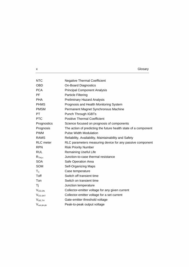
NTC Negative Thermal Coefficient OBD On-Board Diagnostics PCA Principal Component Analysis PF Particle Filtering PHA Preliminary Hazard Analysis PHMS Prognosis and Health Monitoring System PMSM Permanent Magnet Synchronous Machine PT Punch Through IGBTs PTC Positive Thermal Coefficient Prognostics Science focused on prognosis of components Prognosis The action of predicting the future health state of a component PWM Pulse Width Modulation RAMS Reliability, Availability, Maintainability and Safety RLC meter RLC parameters measuring device for any passive component RPN Risk Priority Number RUL Remaining Useful Life RTHj-c Junction-to-case thermal resistance SOA Safe Operation Area SOM Self-Organizing Maps TC Case temperature Toff Switch off transient time Ton Switch on transient time Tj Junction temperature VCE,ON Collector-emitter voltage for any given current VCE,SAT Collector-emitter voltage for a set current VGE,TH Gate-emitter threshold voltage Vout pk-pk Peak-to-peak output voltage

Table of Contents

1 INTRODUCTION ........................................................................................ 23

1.1 PROGNOSIS, PREDICTIVE MAINTENANCE AND PHMS ............................... 25 1.2 HEMIS PROJECT DESCRIPTION .............................................................. 29 1.3 THESIS OBJECTIVES ............................................................................... 34 1.4 PHMS IMPACT AND MAIN FEATURES ....................................................... 35 1.5 METHODOLOGY FOR PHMS DEVELOPMENT ............................................ 36

1.5.1 Identification of failure modes and mechanisms .......................... 39 1.5.2 Identification of failure precursor parameters ............................... 39 1.5.3 Development of on-board systems hardware .............................. 41 1.5.4 Development of accelerated aging tests ...................................... 42 1.5.5 Development of the prognostic algorithm .................................... 43 1.5.6 Algorithm validation ...................................................................... 44

1.6 DOCUMENT STRUCTURE ......................................................................... 44 1.7 REFERENCES ........................................................................................ 46

2 STATE-OF-THE-ART ................................................................................. 51

2.1 PHMS IMPLEMENTATION ........................................................................ 52 2.2 POWER ELECTRONICS RELIABILITY ......................................................... 56 2.3 ACCELERATED AGING TESTS .................................................................. 62

2.3.1 Accelerated Aging Tests on capacitors ........................................ 63 2.3.2 Accelerated Aging Tests on IGBTs .............................................. 65

2.4 PROGNOSIS ........................................................................................... 66 2.4.1 Prognostic models ........................................................................ 71

2.5 PROGNOSIS OF CAPACITORS .................................................................. 73

xii Table of Contents

2.6 PROGNOSIS OF IGBTS ........................................................................... 74 2.6.1 Physics-based models for IGBT prognosis .................................. 75 2.6.2 Data-driven models for IGBT prognosis ....................................... 77 2.6.3 Ensemble methods for IGBT prognosis ....................................... 77

2.7 CONCLUSIONS ABOUT THE STATE-OF-THE-ART ........................................ 78 2.7.1 Conclusions about PHM implementations ................................... 78 2.7.2 Conclusions about Power Electronics Reliability ......................... 78 2.7.3 Conclusions about Accelerated Aging tests ................................. 78 2.7.4 Conclusions about Prognosis in Capacitors ................................. 79 2.7.5 Conclusions about Prognosis in IGBTs ........................................ 80

2.8 REFERENCES ......................................................................................... 82

3 FAILURE MODES & FAILURE PRECURSOR PARAMETERS ............... 91

3.1 ELECTROLYTIC CAPACITOR PHYSICS ....................................................... 92 3.2 ELECTROLYTIC CAPACITOR FAILURE MODES ............................................ 95

3.2.1 Electrolytic capacitors failure mode conclusions .......................... 97 3.3 ELECTROLYTIC CAPACITOR FAILURE PRECURSOR PARAMETERS ................ 97

3.3.1 Conclusions on failure precursor parameters for electrolytic

capacitors monitoring .................................................................................. 98 3.4 INSULATED GATE BIPOLAR TRANSISTORS (IGBT) PHYSICS ...................... 99 3.5 IGBT FAILURE MODES .......................................................................... 104

3.5.1 Chip-related failures ................................................................... 109 3.5.2 Package-related failures ............................................................. 111 3.5.3 IGBT failure mode conclusions .................................................. 114

3.6 IGBT FAILURE PRECURSOR PARAMETERS ............................................ 114 3.6.1 Conclusions on failure precursor parameters for IGBT monitoring ..

.................................................................................................... 116 3.7 GENERAL CONCLUSIONS OF FAILURE MODE AND FAILURE PRECURSOR

PARAMETERS ................................................................................................. 117 3.8 REFERENCES ....................................................................................... 118

4 ACCELERATED AGING TESTS ............................................................. 123

Table of Contents xiii

4.1 CAPACITOR FAILURE PRECURSOR MONITORING HARDWARE .................... 124 4.1.1 Laboratory tests measuring hardware........................................ 125 4.1.2 Onboard monitoring hardware ................................................... 127

4.2 CAPACITORS ACCELERATED AGING MODE ............................................ 139 4.2.1 Constant temperature degradation ............................................ 140 4.2.2 Varying temperature degradation ............................................... 140

4.3 CAPACITORS ACCELERATED AGING TESTS RESULTS ............................. 141 4.3.1 Constant temperature degradation results ................................. 141 4.3.2 Varying temperature degradation results ................................... 144

4.4 IGBT FAILURE PRECURSOR MONITORING HARDWARE ............................. 148 4.4.1 Laboratory tests measuring hardware........................................ 148 4.4.2 Onboard monitoring hardware ................................................... 151

4.5 IGBT ACCELERATED AGING TESTS MODE ............................................ 155 4.5.1 Measurement types .................................................................... 159

4.6 IGBT ACCELERATED AGING TESTS RESULTS ........................................ 162 4.6.2 Degradation mechanisms analysis ............................................ 170 4.6.3 IGBT Accelerated Aging Tests Results Summary ..................... 172

4.7 ACCELERATED AGING TESTS CONCLUSIONS ......................................... 175 4.8 REFERENCES ...................................................................................... 176

5 PROGNOSTIC ALGORITHMS ................................................................ 179

5.1 RUL PREDICTION OF CAPACITORS ....................................................... 180 5.1.1 Particle filter-based prognostics theory ...................................... 182 5.1.2 Capacitor Degradation Model .................................................... 185 5.1.3 Case study of Electrolytic Capacitors ......................................... 188 5.1.4 Results of algorithm application ................................................. 191 5.1.5 Conclusions of capacitor prognosis ........................................... 196

5.2 RUL PREDICTION OF IGBTS ................................................................. 197 5.2.1 Prognostic method ..................................................................... 199 5.2.2 Applying the “Bagging” method for RUL and uncertainty prediction

.................................................................................................... 206

xiv Table of Contents

5.2.3 Case study of IGBTs .................................................................. 208 5.2.4 Results of prognostic algorithms ................................................ 212 5.2.5 Conclusions of IGBT prognosis .................................................. 219

5.3 CONCLUSION OF PROGNOSTIC ALGORITHMS .......................................... 220 5.4 REFERENCES ....................................................................................... 221

6 RESEARCH FINDINGS AND FUTURE WORK ...................................... 227

6.1 FINDINGS OF THE INVESTIGATION .......................................................... 227 6.1.1 Regarding the State-of-the-art .................................................... 228 6.1.2 Regarding the Failure Modes and Failure Precursor Parameters

on electrolytic capacitors and IGBTs ........................................................ 229 6.1.3 Regarding the Accelerated Aging Tests ..................................... 230 6.1.4 Regarding the Prognostic Algorithms ......................................... 231

6.2 FUTURE WORK .................................................................................... 231

7 I. APPENDIX A: INTRODUCTION TO RELIABILITY ENGINEERING ... 233

7.1 RELIABILITY ENGINEERING .................................................................... 233 7.2 REFERENCES ....................................................................................... 239

8 II. APPENDIX B: FEV RAMS ANALYSIS ................................................ 241

8.1 INTRODUCTION..................................................................................... 242 8.1.1 Tolerable Hazard Rate assignment to ASIL ............................... 243

8.2 RAMS ANALYSIS ................................................................................. 244 8.2.1 Generic architecture ................................................................... 244 8.2.2 PHA ............................................................................................ 252 8.2.3 RAMS apportionment ................................................................. 259

8.3 RAMS ANALYSIS CONCLUSIONS .......................................................... 265 8.4 MONTE-CARLO SIMULATIONS THEORY ................................................... 266 8.5 REFERENCES ....................................................................................... 268

9 III. APPENDIX C: ENSEMBLE METHOD UNCERTAINTY ASSESSMENT . .................................................................................................................. 271

Table of Contents xv

10 IV. APPENDIX D: CONTRIBUTIONS TO CONFERENCES AND JOURNALS ..................................................................................................... 275

List of Figures

Figure 1.1. Maintenance intervention policies ................................................................. 28

Figure 1.2. HEMIS Project Concept ................................................................................ 30

Figure 1.3. HEMIS PHMS Concept ................................................................................. 32

Figure 1.4. PHM methodology ........................................................................................ 38

Figure 1.5. Bad monotonicity (Left) and good (Right) ..................................................... 40

Figure 1.6. Bad prognosticability (Left) and good (Right) ................................................ 41

Figure 1.7. Bad trendability (Left) and good (Right) ........................................................ 41

Figure 2.1: HUMS system ............................................................................................... 54

Figure 2.2. Source of stressors for electronic equipment failures (% may vary for different applications and designs [21]). ....................................................... 57

Figure 2.3. Failure distribution on industrial power electronic components [26] .............. 59

Figure 2.4. Fragile components distributed by sector type [26] ....................................... 59

Figure 2.5. Fragile components distribution [27] ............................................................. 60

Figure 2.6. Capacitance variation for thermal overstress [36] ......................................... 64

Figure 2.7. ESR and C variation for EOS [36] ................................................................. 64

Figure 2.8. Framework for prognostics [47] ..................................................................... 70

Figure 3.1. Electrolytic capacitor physical layout ............................................................. 92

Figure 3.2. Electrolytic capacitor model [6] ..................................................................... 93

Figure 3.3. Electrolytic capacitor model [2] ..................................................................... 94

Figure 3.4. Capacitor impedance vs frequency plot ........................................................ 94

Figure 3.5. FMEA electrolytic capacitors [1] .................................................................... 96

Figure 3.6. (a) IGBT schematic [4]; (b) IGBT schematic with parasitic elements [17] ... 100

Figure 3.7. IGBT technologies overview [9] .................................................................. 102

xviii List of Figures

Figure 3.8. IGBT module package overview [22] .......................................................... 103

Figure 3.9. Device (IGBT) FIT rate evolution [22] ......................................................... 104

Figure 3.10. IGBT FMEA for extrinsic mechanisms [25] ............................................... 106

Figure 3.11. Power Cycling capability of IGBT Modules [26] ........................................ 107

Figure 3.12. Cosmic ray caused damage [29] .............................................................. 110

Figure 3.13. Bond-wire lift off process [6] ..................................................................... 111

Figure 3.14. Bond-wire lift off examples [34] ................................................................. 112

Figure 3.15. Bond-wire heel cracking IGBT [5] ............................................................. 112

Figure 3.16. Solder fatigue [6] ...................................................................................... 113

Figure 3.17. Solder fatigue crack propagation [6] ......................................................... 113

Figure 3.18. Pros and cons failure precursor parameters [23] ...................................... 116

Figure 4.1. Phase diagram ........................................................................................... 125

Figure 4.2. Equivalent phase diagram .......................................................................... 126

Figure 4.3. Hartley Oscillator ........................................................................................ 127

Figure 4.4. Bode plot of ESR circuit Matlab .................................................................. 131

Figure 4.5. Simulation circuit schematic ....................................................................... 132

Figure 4.6. Simulated output waveforms: a) Current in the tank; b) OPAMP output voltage; c) Tank output voltage (Vout) ....................................................... 133

Figure 4.7. Bode plot pSpice simulations ...................................................................... 135

Figure 4.8. Experiments waveforms ............................................................................. 136

Figure 4.9. Relationship between Vout in simulations and experiments ....................... 137

Figure 4.10. Prototype PCB .......................................................................................... 137

Figure 4.11. Capacity vs frequency at different degradation cycles .............................. 142

Figure 4.12. ESR vs- frequency at different degradation cycles ................................... 142

Figure 4.13. Capacity variation for 3A and 4A .............................................................. 143

Figure 4.14. ESR variation for 3A, 4A and equation from [7] ........................................ 143

Figure 4.15. Capacity variation with degradation .......................................................... 145

Figure 4.16. ESR variation with degradation ................................................................ 145

Figure 4.17 ESR measurement vs Temperature variation ............................................ 147

Figure 4.18. IGBT Degradation monitoring circuit ......................................................... 149

List of Figures xix

Figure 4.19. IGBT degradation Circuit board ................................................................ 150

Figure 4.20. IR25750 internal schematic diagram [13] .................................................. 153

Figure 4.21. Sensor board ............................................................................................ 154

Figure 4.22. (a) Degradation temperature profile; (b) Current profile ............................ 157

Figure 4.23. Designed inverter ...................................................................................... 161

Figure 4.24. IGBT threshold voltage for (a) IR, (b) FUJI, (c) IXYS ................................ 164

Figure 4.25. IGBTs Vce,sat voltage for (a) IR, (b) FUJI, (c) IXYS ................................. 166

Figure 4.26. IGBTs Vce,sat voltage for continuous degradation for (a) IR, (b) FUJI, (c) IXYS ..................................................................................................... 168

Figure 4.27. (a) Vce voltage for normal conditions (b) Vce value for the same Ic and Tc conditions .............................................................................................. 169

Figure 4.28. (a) Gate-oxide destruction IR (b) and (c) die-attach degradation on IR1 and IR4 (d) and (e) voids and crack propagation on FUJI1 and 4. (f) bond-wire on FUJI5 .................................................................................... 174

Figure 5.1. Sketch of the PF approach to fault prognostics ........................................... 183

Figure 5.2. ESR measurement vs Temperature variation ............................................. 189

Figure 5.3. RUL prediction and corresponding 10th and 90th percentiles. The top Figure refers to a process noise standard deviation of 0.1, the Figure in the middle to 0.2, the bottom Figure to 0.3 ................................................ 193

Figure 5.4. Expected RUL of PF with varying temperature ........................................... 195

Figure 5.5. Expected ESR of PF with varying temperature ........................................... 195

Figure 5.6. Vce,sat evolution with degradation for (a) IR, (b) FUJI and (c) IXYS .......... 200

Figure 5.7. Sketch of the Hybrid Model approach to fault prognostics .......................... 206

Figure. 5.8. Lifetime vs. Delta Tj ................................................................................... 210

Figure. 5.9: Accumulated damage predicted by the physics-based model ................... 210

Figure. 5.10. Data-driven algorithm residuals for IR 4 ................................................... 211

Figure. 5.11. RUL predictions for IR 4 only employing (a) raw data, (b) data-driven models, (c) physics-based model, (d) data-driven and physics-based ....... 216

Figure. 5.12. RUL predictions for (a) IR 6, (b) FUJI 4, (c) IXYS 5 and (d) IR 6 with Mixed data ................................................................................................. 219

Figure 7.1. Bathtub curve .............................................................................................. 235

Figure 7.2. New European Driving Cycle ...................................................................... 237

xx List of Figures

Figure 8.1. ISO 26262 V Process model ...................................................................... 243

Figure 8.2. Generic electric vehicle architecture: functional view ................................. 247

Figure 8.3. Expanded view of Electrical Transmission from architecture functional view ........................................................................................................... 249

Figure 8.4. Hierarchical view of generic Traction Machine ........................................... 251

Figure 8.5.Hierarchical view of generic Power electronics ............................................ 252

Figure 8.6. Functional failure analysis steps ................................................................. 256

Figure 8.7. Undemanded vehicle acceleration fault tree ............................................... 261

Figure 8.8. Structure of Ishikawa diagram .................................................................... 264

Figure 8.9. Ishikawa diagram of Undemanded vehicle acceleration ............................. 265

Figure 8.10. Inverse transform method: continuous distribution ................................... 267

List of Tables

Table 3.1. FMEA for IGBT failures [24] ......................................................................... 105

Table 3.2. CTEs for common electronic materials [27].................................................. 108

Table 4.1. Simulation component values ...................................................................... 132

Table 4.2. Simulation results ......................................................................................... 134

Table 4.3. Results of experiments ................................................................................. 136

Table 4.4. Varying degradation temperature values per week ...................................... 141

Table 4.5. IGBT Nominal Characteristics ...................................................................... 156

Table 4.6. Selected degradation temperature values .................................................... 158

Table 4.7 Number of thermal cycles endured ............................................................... 162

Table 4.8. Accelerated Aging Tests Results Summary ................................................. 173

Table 5.1. Experimental values for α, β and γ parameters ............................................ 189

Table 5.2. Average value of the Performance Indexes AI, PI, SI, RI, COV over the 6 available real ESR measures ...................................................................... 194

Table 5.3. Performance Indexes of RUL prediction for varying temperature ................. 196

Table 5.4. Pseudo code for the hybrid ensemble application ........................................ 208

Table 5.5. Number of thermal cycles endured .............................................................. 209

Table 5.6. Average values of the PI for RUL predictions for IR4 ................................... 214

Table 5.7. Average values of the PI for RUL prediction for IR 4 .................................... 214

Table 5.8. Average values of the PI for RUL prediction of IR 6, FUJI 4, IXYS 4 and IR 6 with mixed data.................................................................................... 217

Table 8.1. Mapping between ASIL of ISO 26262, SIL of IEC 61508, and THR ............. 244

Table 8.2. Classification of severity of functional safety hazards .................................. 254

Table 8.3. Classification of “probability of exposure” to functional safety hazards ........ 254

xxii List of Tables

Table 8.4. Classification of “controllability” of functional safety hazards ....................... 255

Table 8.5. Risk classification criteria ............................................................................. 256

Table 8.6. Hazard analysis and risk classification results: functional (FHAZ_x) and physical (PHAZ_x) safety hazards .............................................................. 258

Table 8.7. Fault Tree Symbols ...................................................................................... 260

Table 8.8. FMECA sample of electrical transmission inverter components .................. 263

Chapter 1

1 Introduction

On United Nations words (2013) [1]: “The human influence on the climate system is clear and is evident from the increasing greenhouse concentrations in the atmosphere. Warming of the climate system is unequivocal, and since the 1950s, many of the observed changes are unprecedented over decades to millennia. The atmosphere and ocean have warmed, the amounts of snow and ice have diminished, sea level has risen, and the concentrations of greenhouse gases have increased.”

Upon the previous negative affirmation, many are the positive counteractions that several countries are trying to implement and develop. One of those is the meaningful employment of natural resources and energy.

From this point of view, transportation is one of the main contributors to the increase of CO2 gas in the atmosphere, accounting for 25% of the total amount of emissions in the EU. Oil based transportation is still the most important one.

In this sense, the EU has developed a bunch of policies to change the trend; i.e. tax reduction for low CO2 emission vehicles, investments on renewable energies and electric and hybrid vehicle development. It is in this last point were great effort has been done, being one of the groups of investment within the FP7 programme of the EU [2]. This research was developed within the European Community funded project called: “HEMIS: Electrical Powertrain Health Monitoring for Increased Safety of FEVs”, which is further explained.

24 Introduction

As a result of this impulse and the introduction of the new policies, car manufacturers are giving steps towards a change for the electrification of road transport; beginning from newly appeared manufacturers such as Tesla motors, to Renault, Audi, BMW, Toyota or Nissan.

FEV has attracted much attention in research communities as well as in the market. In 2011 electric vehicle sales were estimated to reach about 20,000 units worldwide, increasing to more than 500,000 units by 2015 and 1.3 million by 2020, which accounts for 1.8 per cent of the total number of passenger vehicles expected to be sold that year [3].

It is well known that Fully Electric Vehicles (FEV) have some advantages over the conventional internal combustion engine (ICE) vehicles due to the absence of tailpipe emissions, high efficiency, and quiet and smooth operation. Over the last years, EVs have improved significantly in their system integration, dynamic performance, compact design and cost. On the other hand, the reduced autonomy of FEVs compared to ICEs is still a main drawback. The initial costs associated to FEV acquisition and the lack of knowledge on system degradation, and thus, on maintenance costs, have discouraged many potential customers.

The automotive industry is especially affected by systems failure due to the high impact on customers’ image of the brand. Opinion polls show that consumers are concerned about the reliability of FEV technology; reliability is one of the main reasons why potential consumers would choose a hybrid vehicle instead of a FEV [4, 5]. Hence, the business case for electric vehicles is affected by component performance and lifetime issues [2] and any failure in this field can potentially damage consumers’ confidence.

The introduction of FEV in the mainstream has raised concerns on reliability issues regarding the electric and power electronic components [6]. Although the electric machines and associated power electronics have been largely developed in the last decades and their manufacturing processes are well established, their reliability and failure mechanisms are still a pending issue on this type of applications [6, 7, 8]. Indeed, following batteries large space requirement, electric drives design has sought to reduce space, and thus, large power densities and compact design have been the main priorities, negatively influencing the reliability of components, due to higher operating temperatures.

Chapter 1 25

Moreover, extreme and demanding environmental conditions are major challenges for the automotive industry suppliers in general, and so, they add to the mentioned problem.

In this work, in order to improve FEV reliability and safety, the previously presented problems were addressed through the implementation of a Prognostic and Health Monitoring System (PHMS) for the most critical power electronic components.

In the following points of this chapter the origins of PHM are described as well as the interests of introducing this kind of maintenance policies and their fundamentals.

1.1 Prognosis, predictive maintenance and PHMS The origins of prognosis can be found in medicine, applied to humans,

rather than applied to machinery. One of the earliest written works of medicine is the Book of Prognostics of Hippocrates, written around 400 BC. This work opens with the following statement: "It appears to me a most excellent thing for the physician to cultivate Prognosis; for by foreseeing and foretelling, in the presence of the sick, the present, the past, and the future, and explaining the omissions which patients have been guilty of, he will be the more readily believed to be acquainted with the circumstances of the sick; so that men will have confidence to entrust themselves to such a physician." [9]

From the previous statement, it can be derived that Prognosis is related to the health state of components, either a person or a machine. More precisely, based on foreseeing the future state in the presence of a problem and taking into account the past and the present events. Therefore, a major issue of the prognostic system is being able to assess the lifetime and be able to predict or foresee the future health state of the system. In recent years, the implementation of prognostic systems has been done through the development of Prognostic and Health Monitoring Systems (PHMS).

In spite of the long time passed since Hippocrates, PHMS is at an infant stage. Great advances have been done on prognostics in medicine applied to humans, but very few have been done related to machinery. Indeed, it is in the last decade that the name has been recovered and established for these

26 Introduction

applications. The foundation of the PHM Society in 2009 showed the clear increasing interest that is arising around monitoring systems. The introduction of PHM systems has been mainly associated to safety critical applications, such as aerospace, nuclear, military and railway industries. Following the novelty of PHMS, different approaches have been suggested depending on the industry [10].

In [11], PHM is defined as the capabilities of a system that preserves the system’s ability to function as intended. In this way, it addresses the design, development, operation, and lifecycle management of components with the purpose of maintaining nominal system behavior and function and assuring mission safety and effectiveness under nominal conditions.

Now, the different characteristics that PHM operation should enable are described [11]:

1. Efficient fault detection, isolation, mitigation and recovery.

2. Prediction of impending failures or functional degradation.

3. Increased reliability and availability of systems.

4. Enhanced vehicle situational awareness.

5. Condition-based and just-in-time maintenance practices.

6. Increased asset availability.

The fulfillment of all the previous points would mean the application of a whole bunch of management policies to research and apply strict procedures on the lifecycle of products, from design to decommissioning. It is believed that PHM embraces and expands the capabilities of traditional safety and reliability engineering methods. It should not be limited to real-time operation, but it should cover the entire systems lifecycle from design to verification and from operation to logistics [12, 13, 14].

From the previous assessments, the main objective of PHMS is to provide information on the failsafe state of the component and enable the application of a predictive maintenance policy. Furthermore, a PHM system should predict the probability of failure and the Remaining Useful Life (RUL) of

Chapter 1 27

the equipment, thus, providing valuable aid deciding when maintenance actions should be performed to avoid catastrophic failures of the system.

The previous characteristics will lead to improve safety and maintainability, together with a reduction of maintenance costs, which are the highest ones during the operational life of the system [10], due to the enhanced knowledge of failure mechanisms affecting the powertrain.

Since PHMS enables continuously monitoring the system operation, PHMS application can be observed as an advanced maintenance policy. Provided that the PHMS is monitoring the component, it allows replacing the component exactly prior to a failure occurrence, thus, extending to the limit its operative life. The evolution of maintenance policies has been possible due to the understanding of the degradation processes affecting the complex systems that humans have built.

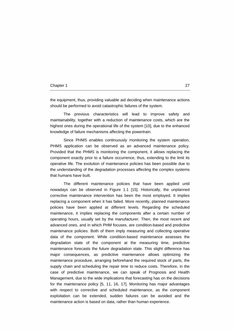
The different maintenance policies that have been applied until nowadays can be observed in Figure 1.1 [15]. Historically, the unplanned corrective maintenance intervention has been the most employed. It implies replacing a component when it has failed. More recently, planned maintenance policies have been applied at different levels. Regarding the scheduled maintenance, it implies replacing the components after a certain number of operating hours, usually set by the manufacturer. Then, the most recent and advanced ones, and in which PHM focuses, are condition-based and predictive maintenance policies. Both of them imply measuring and collecting operative data of the component. While condition-based maintenance assesses the degradation state of the component at the measuring time, predictive maintenance forecasts the future degradation state. This slight difference has major consequences, as predictive maintenance allows optimizing the maintenance procedure, arranging beforehand the required stock of parts, the supply chain and scheduling the repair time to reduce costs. Therefore, in the case of predictive maintenance, we can speak of Prognosis and Health Management, due to the wide implications that forecasting has on the decisions for the maintenance policy [5, 11, 16, 17]. Monitoring has major advantages with respect to corrective and scheduled maintenance, as the component exploitation can be extended, sudden failures can be avoided and the maintenance action is based on data, rather than human experience.

28 Introduction

Nowadays, the knowledge on complex system degradation mechanisms, advances on sensory components, data mining and machine learning techniques, has made it possible to introduce PHM systems and improve maintenance policies. However, PHM system development require high research and investment costs, and so, its employment has been restricted to safety critical applications.

In this sense, PHM application has been avoided in the automotive industry taking into account the associated costs. Still nowadays, corrective maintenance is the leading policy; mainly supported on a vast market of parts making profit from maintenance. Another issue that delays the application of PHMS are confidential clauses. As a consequence of such a competitive market, automakers refuse to publish any data or results of researches related to reliability of components.

As a result, to the author’s best knowledge, the HEMIS project is the first attempt to implement a PHM system on a FEV.

Figure 1.1. Maintenance intervention policies

Chapter 1 29

Nevertheless, car manufacturers have given some steps forward regarding vehicle performance and failure analysis with the introduction of the On Board Diagnostics (OBD) system. The employment of OBD-II system was made mandatory since 1996 for all light vehicles. The OBD system gives the operator access to the status of the various vehicle subsystems. Modern OBD implementations use a standardized digital communications port to provide real-time data and standardized diagnostic trouble codes. The main target was to reduce the repair time and ease the procedure to the repair technician, gathering relevant information provided by the different ECUs within the vehicle. However, this system is not provided with any intelligence, there is not data analytics implemented that could predict a RUL of the components, and it forces letting the vehicle on the garage for inspection. As a result, given the concern of customer’s on FEV reliability and safety, PHM is a trend that is foreseen to become a truth in the near future.

After this brief introduction to prognosis and PHMS, the main features of the HEMIS project are described, as its development greatly influenced the outcome of this work.

1.2 HEMIS Project description The “HEMIS: Electrical powertrain Health Monitoring for Increased

Safety of FEVs” project (www.hemis-eu.org) was a European Community funded project within the 7th Framework Programme with reference number: FP7-ICT-314609, beginning in June 2012 and finishing on February 2015. Seven partners formed the consortium: CEIT-IK4 (Spain), as coordinator of the project, York EMC Services (UK), Applus IDIADA (Spain), VTT (Finland), Politecnico di Milano (Italy), MIRA Ltd. (UK) and JEMA Energy (Spain).

Firstly, the project focused on the problems associated to the previously mentioned advent of FEVs in mass production. This implied immaturity of the new building blocks, which can reduce FEV’s safety and reliability. Among them, the project focused on the electric powertrain, i.e. electric traction motor and the power electronics converter. Another point taken into account by the project was the emitted electromagnetic fields (EMF) analysis, due to the high currents flowing from the battery to the electric motor, including Low Frequency (LF) emissions not covered within current automotive EMC standards.

30 Introduction

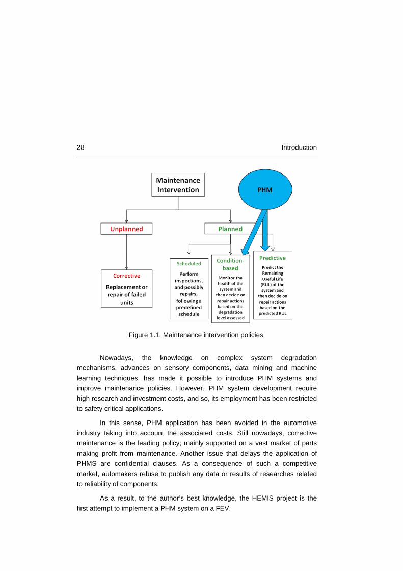
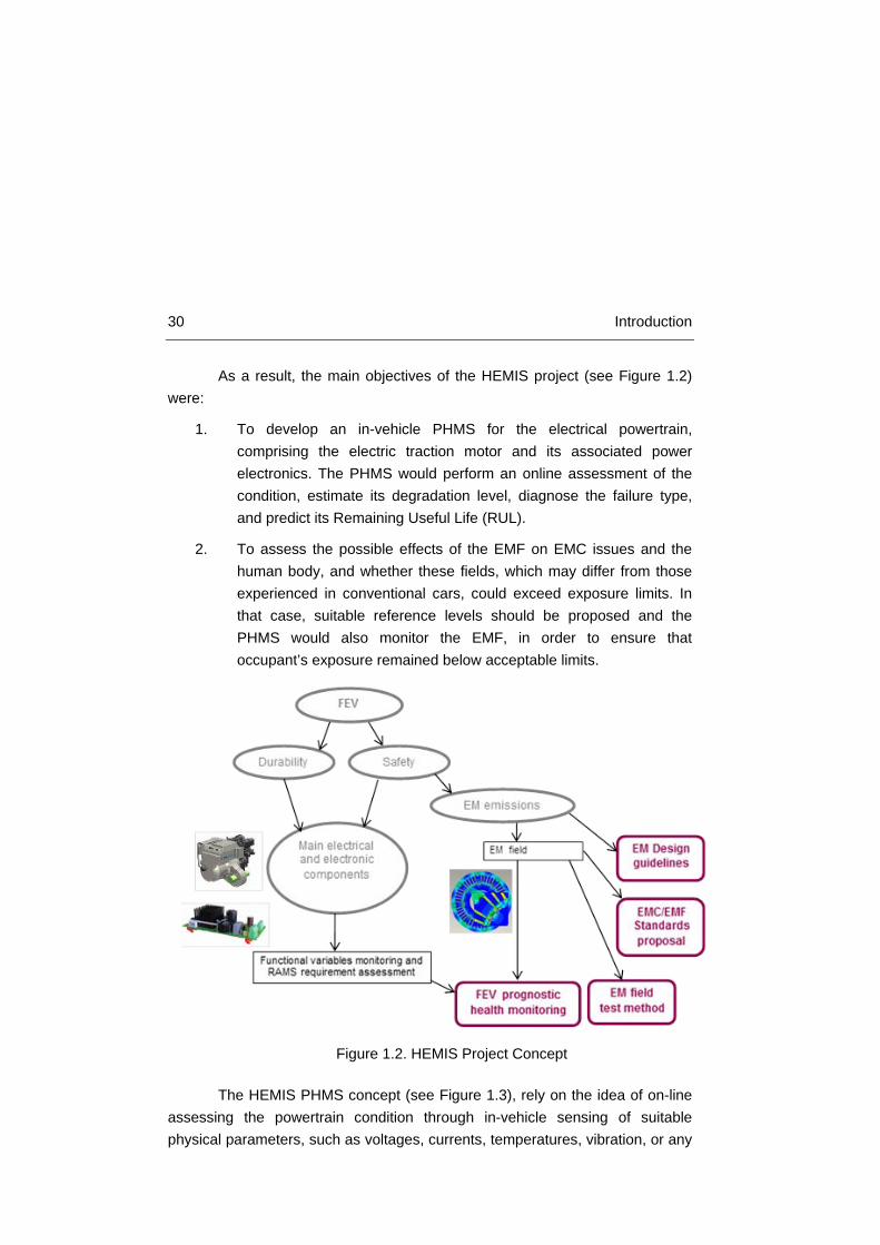
As a result, the main objectives of the HEMIS project (see Figure 1.2) were:

1. To develop an in-vehicle PHMS for the electrical powertrain, comprising the electric traction motor and its associated power electronics. The PHMS would perform an online assessment of the condition, estimate its degradation level, diagnose the failure type, and predict its Remaining Useful Life (RUL).

2. To assess the possible effects of the EMF on EMC issues and the human body, and whether these fields, which may differ from those experienced in conventional cars, could exceed exposure limits. In that case, suitable reference levels should be proposed and the PHMS would also monitor the EMF, in order to ensure that occupant’s exposure remained below acceptable limits.

The HEMIS PHMS concept (see Figure 1.3), rely on the idea of on-line assessing the powertrain condition through in-vehicle sensing of suitable physical parameters, such as voltages, currents, temperatures, vibration, or any

Figure 1.2. HEMIS Project Concept

Chapter 1 31

other relevant variable available. Diagnostic and prognostic algorithms developed within the project would then be used to assess the powertrain health condition and estimate the RUL of its critical components. Therefore, optimizing the maintenance actions and saving costs.

The main features of the PHMS should be:

• Safety. This aspect is essential to increase the safety of the vehicle. The PHM system must have low missing alarm rates. The failure rate of the PHMS should also be low compared to the powertrain in order to be useful.

• Cost-effectiveness. During the project development some industrial representatives formed an Industrial Advisory Panel. It suggested that in order to be an interesting option to be introduced in commercial vehicles the main drawback was the cost of the system. Indeed, the cost of developing and installing the PHMS on the FEV should be repaid by the reduction of the maintenance costs. In this context, false alarm rates should be low to avoid unnecessary stops.

32 Introduction

The project focused on the study of the powertrain of the vehicle, excluding the high voltage batteries from the beginning. The main reason was that projects addressing batteries health state monitoring were already run by other researches. Although HEMIS PHMS intended to be a broad and general application tool, independently of the powertrain architecture (1, or 2 motors, Permanent Magnet or Asynchronous Machines, etc.), it focused on powertrains working with an inverter and a Permanent Magnet Synchronous Machine (PMSM), since it is the most employed architecture in modern FEVs [18, 19, 20, 21].

A key point of the project was the development of a Reliability, Availability, Maintainability and Safety (RAMS) analysis of the FEV. The goals of the RAMS analysis were:

• Identify the most critical functional failures of FEV systems, focusing on the ones derived from the powertrain subsystem.

• Identify reliability critical components of the powertrain subsystem.

• Assess whether the Tolerable Hazard Risk target was fulfilled.

• Evaluate the benefits of introducing the PHMS.

Figure 1.3. HEMIS PHMS Concept

Chapter 1 33

Minimum Endogenous Mortality is a risk acceptance principle which suggests that the introduction of a new system does not significantly contribute to the existing mortality caused by technical systems. In this sense, the target was fulfilled.

RAMS techniques have been extensively applied to the electro-technical engineering field in risk engineering. RAMS techniques allow reliability engineers to forecast failures from the observation of operational field data [22]. RAMS analysis is well-structured, usually based on standards and follows systematic procedures. Different steps are required prior to the RAMS analysis, which are, the definition of the architecture of a generic system i.e. FEV, the preliminary hazards analysis (PHA), the establishment of a tolerable hazard rate and the definition of safety goals. An extract and the description of the main parts of the RAMS analysis, as well as the basic theory of Reliability Engineering, can be found in Appendix I and II. One of the most important tools of RAMS analysis, the Failure Modes and Effect Analysis (FMEA), helped to discover the most critical components of the powertrain. They were found to be:

Most critical components of power electronics converter:

• Insulated Gate Bipolar Transistors (IGBT).

• DC Bus Link Electrolytic Capacitors.

Most critical components of the PMSM:

• Bearings.

• Permanent Magnet field source.

• Stator windings.

In order to quantify and evaluate the improvement on reliability and availability regarding the introduction of a PHMS in the FEV powertrain, Monte-Carlo (MC) simulations were run. This simulation method is extensively employed for complex system reliability and availability modeling [23]. In MC simulations, a logical model of the system being analyzed is repeatedly evaluated. The logical model contains the different states in which the system could be (i.e. working, degraded, failed, etc.). Each run of the simulation, randomly sampled values of the parameters for the transitions are employed.

34 Introduction

The results of the MC simulations were published on [24] and [25]. A description of the MC method theory can be found in Appendix II. A 10 % improvement on reliability was obtained when a PHMS was introduced in the FEV powertrain.

Following the results of the RAMS analysis of the HEMIS project, the starting point of this thesis was set. In order to develop a PHMS the most critical components of power electronics were selected to be further studied. This selection was also supported on the results of other industrial reliability researches (see Chapter 2.2), which draw attention over the same components.

The development of PHMS is not standardized and scarce examples are available in the literature (see Chapter 2.1) for the different industries. Following the introduction that has been done on PHMS and on the HEMIS project, the objectives of this thesis are presented.

1.3 Thesis objectives The main goal and contributions to knowledge of this research are

presented.

• Main goal: Propose and validate a Prognostic and Health Monitoring System (PHMS) for the inverter of a FEV powertrain, in order to improve its reliability, maintainability and safety.

The milestones for the achievement of the main goal are listed below:

o Identification of the main failure modes and mechanisms.

o Identification of the failure precursor parameters.

o Development of on-board systems for failure precursor parameter monitoring.

o Development of accelerated aging tests for experimental data collection.

o Development of the prognostic algorithms.

o Validation of the algorithms on the collected experimental data.

Chapter 1 35

In the next section the selected main features for the PHMS to be developed for the power electronics converter are presented, and then, the methodology is explained.

1.4 PHMS impact and main features Having analyzed the main focus of the research, which is, the

development of a PHM system for the power electronics converter of a FEV powertrain, it can be described the main features for the PHM system.

First of all, the driving objectives and impact of the PHM system must be set. The knowledge of the state of equipment and the ability to predict its future evolution are the basis of condition-based maintenance strategies. According to these strategies, maintenance actions are carried out when a measurable equipment condition shows the need for corrective repair or preventive replacement [10, 26]. From the point of view of equipment safety and durability, by identifying potential problems in the early stages of their development, it is possible to allow the equipment to run as long as it is safe and to opportunely schedule the maintenance interventions. Thus, the driving objectives for PHM design in an automotive application are maximum availability, minimum unscheduled shutdowns and economical maintenance [24, 27].

Taking into account the previous considerations, the proposed PHMS is based on the following features:

1. A set of sensors to monitor key physical characteristics (i.e. currents, temperatures, etc.) related to the health of the power electronic components.

2. Analytical and empirical laws that allow predicting the evolution of the selected physical characteristics. In short, they will allow predicting the Remaining Useful Life (RUL) of the monitored equipment. Consequently, the online RUL estimation should be the main outcome of the methodology.

3. Most critical failures and components must be addressed. Therefore, the failure modes and mechanisms of the monitored components must be deeply studied and understood.

36 Introduction

4. Minimal impact (minimal intrusiveness) on vehicle design and manufacturing [27]. Sensor layout, wiring and control boards included within the PHM system, must be optimized to minimize the need for modifications of the adjacent structure and topology of the integrated systems within the car. Non-intrusive sensors and components are desired, in order to reduce the complexity and the mounting process of the items.

5. The system must be reliable and robust. Firstly, it is expected that the PHM system lifecycle itself will be longer than the monitored system. Besides, the false positive and false negative cases need to be small in order to be a trustworthy system. Automotive industry is highly concerned on new system introduction unless it has been well tested.

6. Minimum and optimized cost. This feature implies simplified and reduced hardware.

In short, the PHMS consists of:

1. Hardware monitoring variables related to the degradation process of components.

2. Prognostic algorithms which predict the Remaining Useful Life (RUL) of the components based on the measured data.

Taking into account the results of the HEMIS project and the analysis of the Reliability of Power Electronic components in Chapter 2.2, the selected items to be monitored by the PHMS are:

1. Electrolytic Capacitors.

2. Switching Semiconductor Devices.

Now, a detailed description of the methodology that has been followed for PHMS development is presented.

1.5 Methodology for PHMS development Once the objectives and main features of the PHMS have been set, the

methodology that has been followed to develop the PHMS is explained.

Chapter 1 37

The development of a PHMS for a new technological design such as the power electronics converter of a FEV powertrain is a complex task which requires the management of multiple and hybrid sources of information and knowledge, i.e. expert judgment, analytical models of degradation mechanisms and experimental data [28]. In order to do so, a systematic procedure for the development of the PHMS is presented.

As it has been previously introduced, since dealing with an immature technology whose functional behavior has not been completely tested, the first step of the system analysis should be the identification of the most critical components and the corresponding failure modes. In this sense, RAMS analysis, and more precisely, FMECA tool with the computation of the Risk Priority Number (RPN) are of major importance [29, 30].

Once the most critical components and their failure modes have been identified, it is necessary to investigate the degradation mechanisms which cause the identified failure modes. This analysis provides a physical point of view on the degradation process occurring in the system, augmenting the comprehension of the system possible behavior. Then, it is necessary to select the signals to be measured in order to monitor the health state, the so-called failure precursor parameters. This selection is driven by both physical and economic considerations, taking into account whether it is physically possible to measure a specific signal, the precision required and the cost of the measurement system.

At that point, once the data is available and the knowledge of the physical laws driving the degradation process is known, the development of the PHM algorithms can be started. Depending on the characteristics of the degradation mechanisms (i.e. sudden or gradual), the objective can be the diagnosis or the prognosis of the failure. The diagnostic system would provide a detection of the onset of a component anomalous behavior and the identification of its causes. Meanwhile, a prognostic system aims at the prediction of the system RUL. The availability of degradation data or physical degradation models drives the choice of the monitoring algorithms, which can be model-based, data-driven or hybrid.

Finally, in order to verify the performance of the developed algorithms, a validation strategy must be defined. In this case, the verification process has

38 Introduction

been done through testing the algorithm with real experimental data and checking the results with performance indexes.

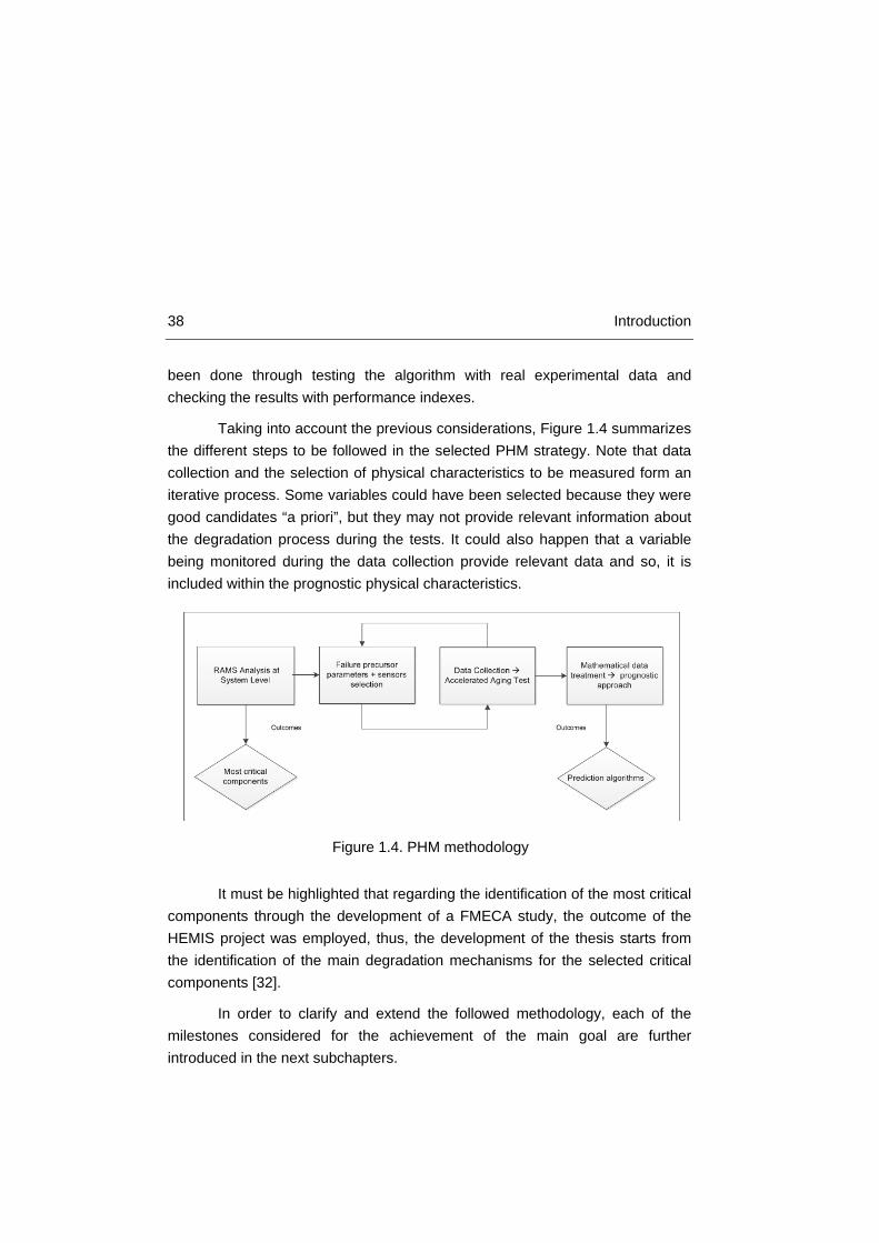
Taking into account the previous considerations, Figure 1.4 summarizes the different steps to be followed in the selected PHM strategy. Note that data collection and the selection of physical characteristics to be measured form an iterative process. Some variables could have been selected because they were good candidates “a priori”, but they may not provide relevant information about the degradation process during the tests. It could also happen that a variable being monitored during the data collection provide relevant data and so, it is included within the prognostic physical characteristics.

It must be highlighted that regarding the identification of the most critical components through the development of a FMECA study, the outcome of the HEMIS project was employed, thus, the development of the thesis starts from the identification of the main degradation mechanisms for the selected critical components [32].

In order to clarify and extend the followed methodology, each of the milestones considered for the achievement of the main goal are further introduced in the next subchapters.

Figure 1.4. PHM methodology

Chapter 1 39

1.5.1 Identification of failure modes and mechanisms The main failure modes and mechanisms for the electrolytic capacitor

and semiconductor devices have been studied through a literature review. Once the failure modes are clear, it is necessary to identify the corresponding responsible degradation mechanisms. This is a complex task, as degradation processes are closely related to physical characteristics of materials, mechanical properties, package technologies and manufacturing processes. Therefore, this task has required the analysis of the failure mode from a physical point of view.

In this sense, a deep review on components physics has been done. Then, the failure mechanisms reported by other researches were analyzed. Information coming from experts or the analysis from failures in similar components was considered. If several degradation mechanisms cause the same failure mode (i.e. short circuit) the most likely to occur should be identified and the successive analysis focus on it.

1.5.2 Identification of failure precursor parameters The objective of this step is to identify those physical characteristics

which can provide useful information to the PHM for monitoring the component degradation state and predicting its useful life. With the term failure precursor parameters, signals that can be measured thanks to sensors and which are correlated to the health state or which describe the component operation mode and environment is meant. Operation mode and environmental variables should be considered since it has been shown that they can have a strong impact on component degradation [10].

This step is performed by firstly identifying a list of possible physical characteristics by considering the following sources of information:

• Information and knowledge on the degradation process, such as, signals used in analytical and/or empirical models of the degradation process.

• Expert judgment on factors that may influence the component degradation state.

40 Introduction

• Literature review.

Once the candidate physical characteristics have been identified the final selection of those to effectively predict the component RUL is driven by the following considerations:

• The possibility of predicting the components RUL using the proposed physical characteristics.

• An assessment of the feasibility and cost of performing the measurements, their accuracy and the complexity of the data processing.

With respect to the detection of the system degradation, physical characteristics which have different behaviors in case of normal operation or in case of system degradation are searched. Prognosis requires that the measurements collected during the degradation process leading to different failure modes should show clear trends and patterns, appearing in different zones of the space formed by the physical characteristics.

Finally, with respect to the prognostic task, the following three properties of the physical characteristics are desirable [33]:

• Monotonicity: physical characteristics are wished to present an overall positive or negative trend in time.

• Prognosticability: the distribution of the final value that a physical characteristic takes at failure is wished to be “peaked”, i.e. not too wide-spread.

Figure 1.5. Bad monotonicity (Left) and good (Right)

Chapter 1 41

• Trendability: the entire histories of evolution of the physical characteristics towards failure are wished to have quite similar underlying shapes, describable with a common underlying functional form.

1.5.3 Development of on-board systems hardware Once the physical characteristics to be monitored are selected “a priori”,

sensor boards to monitor them online should be designed. In order to do so, the main features to be considered in the PHMS shall be considered, i.e. minimum intrusiveness, minimum cost, required accuracy levels, etc.

It needs to be taken into account during the boards’ component selection process the required accuracy, as well as the variation of the signals due to external environmental effects. The variations in the measurements due to the measuring system could introduce noise, and, if big enough, it could avoid observing the underlying degradation patterns.

Figure 1.7. Bad trendability (Left) and good (Right)

Figure 1.6. Bad prognosticability (Left) and good (Right)

42 Introduction

1.5.4 Development of accelerated aging tests This is a critical point of the development and validation process of the

PHMS. Data coming from the degradation process of components may be required for each one of the following actions:

• Check whether the selection of the degradation mechanisms and failure modes is correct.

• Assessment of the real effect of the degradation on the selected precursor parameters.

• Development of the prognostic algorithm, i.e. data-driven models.

• Validation of the prognostic algorithm.

It can be observed that the employment of data regarding components degradation is of vital importance. Three are the major possible sources of data.

• Open-access databases developed by the research community are one of them. Databases regarding bearing degradation [35] or even IGBT degradation [34] have been found. However, it is crucial, in order to develop the prognostic algorithms, to know in which conditions the tests have been run. This is not always available, or even they may suffer from missing data.

• Data provided by the manufacturer. An agreement with the manufacturer of components can be negotiated. However, reliability issues are usually internally and confidentially treated in companies, and thus, access to those sources of information is rare.

• The development of accelerated aging tests. Accelerated aging tests are a common practice for data collection regarding components degradation for reliability and durability testing. The objective is to obtain degradation data results in a reduced period of time. The procedure is to apply stresses well in excess of those that will be seen during the service period. Thus, failures are caused to occur much faster, typically, several orders of magnitude less than would be observed in service.

Chapter 1 43

No agreements were possible with manufacturers due to confidentiality issues. The studied open-access databases did not provide with the desired amount of information. As a result, accelerated aging tests were developed on selected components in this research. The procedure is later explained. As a final consideration, a selection of components is required in order to develop the tests.

The selected capacitor was a general purpose electrolytic capacitor, ALS30 series from KEMET [36]. This capacitor model was selected due to its similarity to the ones employed in FEVs, following the same physical structure [8]. The selected capacitor rated values were a maximum voltage of 100 V and 2200 uF of capacity. The manufacturer assures 20,000 h of operation under rated voltage and current values for a nominal temperature of 85 ºC.

Accelerated aging tests were also developed for semiconductor devices test case. The selected semiconductor device was IGBTs, as it is the one most employed in FEVs (see Chapter 2). Three different types of discrete IGBTs were selected for testing: IR’s IRG4BC30KDpbf punch-through IGBT, FUJI’s FGW15N120VD Trench Field-Stop IGBT and the IXYS IXXN110N65C4H1 Trench XPT GenX4 IGBT. The IR IGBT was selected in order to compare the results with those from previous studies on accelerated aging tests [37] and to validate the selected methodology. The other two IGBT types were selected to represent new IGBT technologies. The FUJI and IR IGBTs have similar packages and nominal currents. The IXYS IGBTs are characterized by a higher nominal current than the other two types. These three IGBT types were selected taking into account that they could be employed in a FEV, although the IXYS is the IGBT with higher current rating, and thus, the one with more possibilities to be embarked on a real inverter. The differences between the three selected IGBT technologies are explained on Chapter 3.

1.5.5 Development of the prognostic algorithm The objective of this step is the practical implementation of the PHM

algorithms. The nature of this algorithm strictly depends on the characteristics of the degradation mechanisms and the data available. According to this, the prognostic algorithms which predict the system RUL depend on the type and sources of data obtained by the accelerated aging tests. Furthermore,

44 Introduction

depending on the availability of physical degradation models, or degradation data, or both, the PHM algorithms could be model-based, data-driven or hybrid, respectively.

1.5.6 Algorithm validation Once the algorithms have been developed, different strategies could be

followed to validate them. The different options are listed below:

1. Testing of the algorithm with data from simulated data. This could be done on the first stages of the algorithm development, if no real data is available.

2. Testing of the algorithm with data from accelerated aging tests. This would be a more close-to-reality approach; thus, if the tests are successful, the algorithm is highly probable to work on real applications.

3. Testing of the algorithms with real data collected during operation of the component on the final application. This last validation is only possible if the final test equipment is built and can be introduced within the vehicle.

In this research, the validation of the algorithms was done following the second validation process, given the lack of a final prototype to be tested within a car, although it would have been the ideal solution. Nevertheless, the application of the proposed validation strategy is able to provide reliable information about the effective applicability of the developed algorithm to the real operation of the system and to quantify its performance.

1.6 Document structure The chapters of the thesis follow the same organization as the

objectives except for Chapter 2. These are:

Chapter 2 studies the state-of-the-art for prognosis of the power electronic components of the FEV powertrain.

Chapter 1 45

The identification of the main failure mechanisms and the selection of the failure precursor parameters to be monitored are included in Chapter 3.

Chapter 4 explains the development of the experimental tests and a description of the hardware employed.

The development and validation of prognostic algorithms for Remaining Useful Life (RUL) estimation of components is explained in Chapter 5.

Chapter 6 contains the conclusions of the research.

46 Introduction

1.7 References [1] T.F. Stocker. “Climate change 2013: the physical science basis: Working

Group I contribution to the Fifth assessment report of the Intergovernmental Panel on Climate Change,” Cambridge University Press. 2014

[2] N. Hill, C. Brannigan, R. Smokers, A. Schroten, H. Van Essen and I. Skinner, “eu Transport ghg: Routes to 2050 ii. Final Project Report Funded by the European Commission’s Directorate-General Climate Action,” Brussels, 2012

[3] B. Ji, “In-situ Health Monitoring of IGBT,” PhD Thesis, Newcastle University, 2011

[4] J.S. Krupa, D.M. Rizzo, M.J. Eppstein, D.B. Lanute, D.E. Gaalema, K. Lakkaraju and C.E. Warrender, “Analysis of a consumer survey on plug-in hybrid electric vehicles,” Transportation Research Part A: Policy and Practice, vol. 64, pp. 14-31, 2014

[5] B. Caulfield, S. Farrell and B. McMahon, “Examining individuals preferences for hybrid electric and alternatively fuelled vehicles,” Transport Policy, vol. 17, issue 6, 381-387, 2010

[6] A. Hensler, J. Lutz, M. Thoben and K. Guth. “First power cycling results of improved packaging technologies for hybrid electrical vehicle applications,” Integrated Power Electronics Systems (CIPS), 2010 6th International Conference on, pp. 1, 2010

[7] F. Adams and A.J. Brock, “Hippocratic writings,” Encyclopaedia Britannica, 1995

[8] Y. Song and B. Wang, “Survey on Reliability of Power Electronic Systems,” Power Electronics, IEEE Transactions on, vol. 28, no. 1. 2013

[9] I. K Jennions, “Integrated vehicle health management: perspectives on an emerging field,” Training, vol. 2009, pp. 9-12. 2011

[10] M. Pecht, “Prognostics and health management of electronics,” Wiley Online Library, 2008

[11] S.B. Johnson, T. Gornley, S. Kessler, C. Mott, A. Patterson-Hine, K. Reichard and P. Scandura,; “System Health Management with Aerospace Applications,” Wiley Online Library, 2011, ISBN: 978-0-470-74133-7

Chapter 1 47

[12] Integrated Vehicle Health Management. Technical Plan, Version 2.03, NASA

[13] J.J. Fox and B.J. Glass. “Impact of integrated vehicle health management (IVHM) technologies on ground operations for reusable launch vehicles (RLVs) and spacecraft,” Aerospace Conference Proceedings, 2000 IEEE, 2000

[14] M. Schwabacher, J. Samuels and L. Brownston. “NASA integrated vehicle health management technology experiment for X-37,” AeroSense 2002, 2002

[15] M. Pecht, “Product Reliability, Maintainability, and Supportability Handbook,” CRC Press, ARINC Research Corporation, 1995, ISBN: 0-8493-9457-0

[16] N.M. Vichare and M. Pecht, "Prognostics and health management of electronics," Components and Packaging Technologies, IEEE Transactions on, vol.29, no.1, pp.222-229, March 2006 doi: 10.1109/TCAPT.2006.870387

[17] A. Ramakrishnan and M. Pecht, “A life consumption monitoring methodology for electronic systems,” Components and Packaging Technologies ,IEEE Transactions on, vol. 26, no. 3, pp. 625–634, Sep. 2003

[18] C.C. Chan, “The State of the art of Electric Vehicles,” Proceedings of the IEEE, Vol. 95, No. 4, April 2007

[19] G. Wu, X. Zhang and Z. Dong; “Powertain architectures of electrified vehicles: Review, classification and comparison,” Journal of the Franklin Institute, vol. 352, 2015, pp. 425-448, 2014

[20] K. Rajasherkara, “Present Status and Future Trends in Electric Vehicle Propulsion Technologies,” Emerging and Selected Topics in Power Electronics, IEEE Journal of, vol. 1, no. 1, march 2013

[21] J. de Santiago, H. Bernhoff, B. Ekergard, S. Eriksson, S. Ferhatovic, R. Waters, M. Leijon; “Electrical Motor Drivelines in Commercial All-Electric Vehicles: A Review,” Vehicular Technology, IEEE Transactions on, Vol. 61, no. 2, 2012

[22] E.J. Henley, H. Kumamoto, “Probabilistic Risk Assessment,” IEEE Press, 1991

[23] P. O’Connor and, A. Kleyner; “Practical reliability engineering,” John Wiley & Sons. ISBN: 0-470-84463-9, 2011

48 Introduction

[24] P. Baraldi, F. Barbissotia, R. Capannaa, S. Colomboa, M. Rigamonti, and E. Zio, “Assessment of the Performance of a Fully Electric Vehicle Subsystem in Presence of a Prognostic and Health Monitoring System,” Chemical Engineering, vol. 33, pp. 787-792, 2013

[25] B. Sedano, D. Astigarraga, P. Baraldi and M. Rigamonti “Assessment of the improvement of the safety and reliability embedding an Electrical Powertrain Health Monitoring in a FEV,” European Electric Vehicle Congress Brussels, Belgium, December 3-5, 2014

[26] S. Mishra, M. Pecht and D.L. Goodman. “In-situ sensors for product reliability monitoring,” Symposium on Design, Test, Integration, and Packaging of MEMS/MOEMS 2002, vol. 4755, pp. 10–19, 2002

[27] J. Finda and R. Hendl; “On- board SHM System Architecture and Operational Concept for Small Commuter Aircraft,” European Conference of the Prognostics and Health Management Society 2014, 2014

[28] M. Jouin, R. Gouriveau, D. Hissel, M.C. Péra, N. Zerhouni, “Prognostics and Health Management of PEMFC – State of the art and remaining challenges,” International Journal of Hydrogen Energy, vol. 38, no. 35, pp. 15307-15317, 2013

[29] J.B. Bowles, “The new SAE FMECA standards,” Reliability and Maintainability Symposium, 1998. Proceedings., Annual, pp. 48-53, 1998

[30] J.B. Bowles, “An assessment of RPN prioritization in a failure modes effects and criticality analysis,” Reliability and Maintainability Symposium, 2003. Annual. pp. 380-386, 2003

[31] P. Baraldi, D. Maio, M. Rigamonti, E. Zio, A. Galarza, D. Astigarraga, and S. Rantala, “A procedure for practical prognostics and health monitoring of fully electric vehicles for enhanced safety and reliability,” in Hybrid and Electric Vehicles Conference (HEVC 2014), 5th IET, pp. 1-7, IET, November 2014

[32] B. Sedano, A. Ruddle, I. Unanue, L. Low, D. Astigarraga, I. Ibarra and A. Galarza, “HEMIS: electrical powertrain health monitoring for increased safety of FEVs,” Chemical Engineering Transactions, vol. 33, 2013

Chapter 1 49

[33] E. Zio “Prognostics and Health Management of Industrial Equipment, Diagnostics and Prognostics of Engineering systems: Methods and Techniques,” Seifedine, Kadry, pp. 333-356, 2012

[34] J. Celaya, P. Wysocki, and K. Goebel, "IGBT accelerated aging data set," NASA Ames Prognostics Data Repository, [/tech/dash/pcoe/prognostic-data-repository/], NASA Ames, Moffett Field, CA., 2009

[35] P. Nectoux, R. Gouriveau, K. Medjaher, E. Ramasso, B. Morello, N. Zerhouni, C. Varnier, “PRONOSTIA: An Experimental Platform for Bearings Accelerated Degradation Tests,” IEEE International Conference on Prognostics and Health Management, Denver, CO, USA, 2012

[36] ALS30 series datasheet. Available on: http://www.kemet.com/Lists/ProductCatalog/Attachments/389/KEM_A4031_ALS30_31.pdf

[37] N. Patil, J. Celaya, D. Das, K. Goebel and M. Pecht;, "Precursor Parameter Identification for Insulated Gate Bipolar Transistor (IGBT) Prognostics," Reliability, IEEE Transactions on, vol.58, no.2, pp.271-276, June 2009

Chapter 2

2 State-of-the-art

In the previous chapter, the motivation of the present work and an introduction to PHMS were presented, as well as the methodology that will be followed for its implementation. However, several points are still missing to fully understand the benefits of introducing a PHMS in a vehicle. The state-of-the-art on the different topics that will be discussed needs to be presented before explaining the contributions of this research. The state-of-the-art is splitted in the following steps:

1. PHMS implementations. The different examples available about PHM systems are reviewed.

2. Power electronics reliability. The aim is to understand why power electronics and which parts may need to be monitored.

3. Accelerated Aging Tests. The different possibilities to develop the accelerated aging tests to collect data regarding component degradation process will be reviewed.

4. Prognosis. The different approaches to prognosis of components life will be reviewed.

52 State-of-the-art

2.1 PHMS implementation Prior to the explanation on the different PHM implementations, it must

be introduced the origins that derived into the evolution for PHM systems. PHM systems are the consequence of the researches developed in the risk and reliability engineering fields in order to assess the lifetime of components. In this sense, reliability analysis has been related historically to predictions with an unknown uncertainty about a components life, therefore, predictions with poor confidence. Now, the advances on the knowledge of the degradation physics, sensory systems and mathematical algorithms allow making optimized predictions, thus reducing the uncertainty.

The origin of the modern meaning of reliability comes from the World War II (WWII). The U.S. military meant by reliability “that a product would operate when expected”, which is nowadays more related to “mission readiness”. Later, the definition of reliability evolved into: “the ability of an item to perform a required function under stated conditions for a stated period of time” [1].

During the WWII big issues arose from the inherent unreliability of electronics and fatigue issues, due to the new manufacturing processes. As a result, major effort was put by the Department of Defense (DoD) into improving the reliability and the quality of the products in the whole manufacturing process and supply chain. Later, that philosophy was exported by J. R. Juran and W. E. Deming to Japan and created the so-called “Japanese quality revolution”, applying the principles of “total quality management”. In 1952, the Advisory Group on Reliability of Electronic Equipment (AGREE) was set in the US. AGREE concluded that in order to break with the high ownership costs due to low reliability, disciplines must be laid down as integral activities in the development cycle. This mainly implied increasing the component testing hours prior to selling. The AGREE report was set as the US Military Standard (MIL-STD 781) [2]. From that moment on, most of reliability predictions were based on handbooks.

Reliability prediction for electronic equipment using handbooks can be traced back to MIL-HDBK-217, published in 1960, which was based on fitting the curve of a mathematical model to historical field data to determine the constant failure rate. Traditional reliability prediction methods for electronic

Chapter 2 53

products include Mil-HDBK-217, 217-PLUS, Telcordia, PRISM and FIDES databases. However, posterior studies recommended avoiding them, as they provide misleading predictions which can result in poor designs and logistics [3].

Handbook based reliability prediction was overcome when in 1992, the U.S. Army Material Acquisition Activity (AMSAA) and the Center for Advanced Life Cycle Engineering (CALCE) spoke to the Department of Defense (DoD) about the problem of the current standards. After that, the AMSAA and CALCE started working with the IEEE Reliability Society to develop a new Standard for Reliability Prediction of Hardware. The outcome from that partnership was the IEEE Std 1413, which proposes a framework with guidelines for the correct implementation of electronic hardware reliability prediction [1, 4]. The purpose of the standard is to “identify the elements for an understandable and useful reliability prediction”, so that a prediction in compliance with the standard will identify critical pieces of information necessary for a user of the prediction to determine the accuracy, uncertainty, and, ultimately, value of the prediction.

Having said that, when reliability predictions are not accurate enough, online monitoring systems that warn of the degradation state of the equipment has been used, in order to improve the reliability. These systems called PHM have been used in different applications which are reviewed now.

One of the first applications at system level can be found on aerospace industry [5]. The so-called Integrated Vehicle Health Management (IVHM) project at NASA, which started in 2009, had the following title: “Automated detection, diagnosis, prognosis to enable mitigation of adverse events during flight.” This system was embarked and tested on the Space Shuttle, Deep Space-1, X-33, X-34 and X-37; and it is still under development for the NextGen programme.

The three elements that compose flight IVHM are advanced sensors, distributed data acquisition architecture with storage and extensive real-time distributed data processing by system health diagnostic algorithms. The diagnostic algorithms are a key point of the system, including Livingstone software [6]. Livingstone is a model-based inference engine that reasons about system-wide interactions to detect and isolate failures. It relies on models of system structure and definitions of nominal behavior, in comparison with actual system behavior to identify and isolate current and predicted future faults.

54 State-of-the-art

However, the IVHM system is not a stand-alone application working on the space, but an “integrated” system, which implies a ground IVHM as well. The information is sent to a control room with advanced applications and automated information processing systems.

On company’s words, the incorporation of the IVHM into the launch vehicle and spacecraft design would mean a potential for significant savings in operations costs. Three were the main objectives. First addressed objective was more autonomous operation in flight and on the ground, which directly translates to reduced workload on the ground controller team through reduction of raw vehicle data into “health summary information”. Secondly, a reduced ground processing of reusable vehicles was sought due to more performance of system health checks in flight, as well as more automated ground servicing. Lastly, safety and reliability were enhanced due to increased capability to monitor system health using modern sensing systems.

Therefore, we could take IVHM as a primary example of the implementation of an onboard PHM system with clear focus on the improvement not only in the maintenance costs, but also in safety and reliability.

Figure 2.1: HUMS system

Chapter 2 55

Another application of a PHM system called pHUMS – Prognostic Health and Usage Monitoring of Military Land Systems, was developed by nCode International [7] (Figure 2.1). Its main objective was to improve operational capability by providing enhanced decision support information on the operational condition of ground vehicles. That information was key to: a. ensure the most reliable vehicles were deployed; b. establish supply of necessary replacement components; c. rapidly identify aging or damaged onboard systems. Three were the elements composing the system: a network of sensors, an onboard processor and an off-board server. They can be seen in Figure 2.1.

Two were the tasks of the HUMS system: diagnosis and prognosis. In the diagnostic task the system was focused on detecting the presence of a fault. On the prognostic task it was focused on predicting the residual life of a component independently from the presence of a fault. The failure of only mechanical systems was addressed.

PHM systems are also expanding on aircraft industry. One of the first commercially available systems was developed by the U.S. Air Force. A system completely focused on semiconductor prognostics was developed by the U.S. Air Force Ridgetop Group, InstaCell [8]. Given the lack of a general approach to semiconductor device reliability, the Cell was designed to reside on-chip with the host application. The Cell captured the real environmental and operating conditions with a family of sensors. The gathered information provided the prognostic cell with the capacity to replicate the behavior of the transistors employed in the host application and make the output useful in determining the effects of the stresses on the application’s performance and service life.

A broad portfolio of products is being offered regarding different aircraft technologies by Honeywell. Under these circumstances, they realized about the operative costs of stopped helicopters. They developed a PHM system also called HUMS for rotor bearing state monitoring, based on accelerometers and a central system with intelligence. HUMS monitors the health of vibrating and spinning parts, and records the operational context of events so that flight and maintenance crews can analyze trends and perform condition-based maintenance.

56 State-of-the-art

Regarding the automotive industry, as it has been previously claimed, no real application cases of PHMS have been found. Nevertheless, it is known that car manufacturers find appealing the benefits of PHMS; Chevrolet has been the first manufacturer to announce that a prognostic system will provide feedback information to the driver about different aspects of the car. The system is announced to be accessible since 2016 for some of their customers. All in all, some tests have been developed regarding electronic products reliability on in-vehicle environments, such as [9] and [10].

As an example of the interest of automotive manufacturers on PHMS, the patents published in recent years can be taken [11-16]. They all are focused on diagnostic and prognostic ideas applied to both hybrid and electric vehicles in particular [14]. The patents suggest in most cases the employment of sensors and advanced algorithms for RUL prediction. Vehicles would be connected to the Internet and real-time information could be collected to inform the driver on any issue. Daimler, Ford, Toyota and General Motors are listed as assignees of the patents. Another remarkable fact is the appearance of IBM, which might be a subcontractor for data analytics and data mining with prognostic objectives.

2.2 Power Electronics Reliability Now that different PHM applications have been shown, the interest on

monitoring the power electronic components of a FEV needs to be explained. There is a wide perception on car consumers that the electronics reliability is low [17]. This perception has spread among consumers for the electric vehicle case, being reliability one of the main reasons why potential consumers would choose a hybrid vehicle instead of a FEV [17]. In order to understand the focus on power electronic components the results of surveys about reliability in industrial applications will be reviewed, due to the lack of experimental results on real FEVs.

To begin with, the employment of power electronic components on FEVs will be explained. Power electronics are not present only on the DC/AC converter (inverter) for electric motor driving. Despite, they can be found in the battery charger as an AC/DC converter. A DC/DC converter could also be employed to increase the battery voltage in order to feed the inverter of the motors, and thus, reduce the current flow. DC/DC converters are also employed

Chapter 2 57

to reduce the main battery voltage to feed the low voltage systems, such as the Electronic Control Units (ECUs). The wide variety and importance of the applications of power electronics on FEVs suggest the improvement on cost savings that their monitoring could carry.

Nevertheless, we will focus on the inverter for the electric motor, as it is a key component for functional operation of the powertrain and the operative loads that it suffers are the biggest ones within the car. The inverter provides with power the traction motor, which implies high temperature variations and highly dynamic conditions. The fact that it operates within a car provides some added sources of damage: high cooling system temperatures, vibrations, shocks, particular thermal and humidity conditions, etc. Therefore, they all affect the components degradation, reducing their life time and compromising overall system reliability [18, 19, 20]. The published reports concerning power electronic failures [21] explain that a powertrain must cope with vibrations and changes of humidity and ambient temperatures, which are source of stressors for electronic equipment failures as shown in Figure 2.2.

Figure 2.2. Source of stressors for electronic equipment failures (% may vary for different applications and designs [21]).

A DC/AC converter system topology commonly employed in FEV operation consists of a filtering capacitor in the input of the DC supply, power switching semiconductor devices, a power converter control board with its

58 State-of-the-art

switching strategy and the drivers, and usually, a closed-loop control system of the motor. The selection of the previous attributes and final system integration is of utmost importance for the development of efficient and high-performance vehicles. The challenges of power electronic converters for FEV applications lie in obtaining a high-efficient, rugged, small sized and low-cost system. Most of the current FEV and HEVs use a three-leg bridge inverter topology with hard switching methodology for converting the dc voltage of the battery to alternating voltage to power the motor [18, 19, 22, 23].

A critical point of inverter design is the semiconductor device selection [24]. With the advancement of semiconductor device technology, several types of power devices with varying degrees of performance are available in the market. In the past, the selection of components was done through expert knowledge and the employment of application notes. Now, semiconductor device manufacturers already provide component selection tools depending on the constraints of the application. These new selection tools only require the introduction of the operating parameters (duty cycle, ambient temperature, cooling system temperature, load power, voltage range, etc…) and they select the right component for the application. Examples of these tools are IPOSIM from Infineon Technologies and Semisel from SEMIKRON.

One of the first FEVs designed for mass production, the IMPACT, was made by General Electric in 1990. It employed 144 MOSFETs per inverter [20]. Each inverter had 24 MOSFETs connected in parallel, in order to carry the required current. Later, the 24 were replaced by a single IGBT. Currently, IGBT devices are being used in almost all commercially available FEVs and HEVs [25]. The IGBTs will continue to be the leading technology in the near future until the silicon carbide (SiC) and gallium nitride (GaN)-based devices are commercially available at a cost similar to IGBTs [74]. Much expectation has been placed on these devices, which are still under research.

Reliability of power electronics is now studied. There have been industrial surveys on power converter reliability in order to determine the most fragile components. Figure 2.3 shows that capacitor and semiconductor failures in power modules account for a total 51 %, according to a survey based on over 200 products from 80 companies [26].

Chapter 2 59

Figure 2.4 shows the results of the survey carried in [26], distributed depending on the industry.

Figure 2.4. Fragile components distributed by sector type [26]

Figure 2.3. Failure distribution on industrial power electronic components [26]

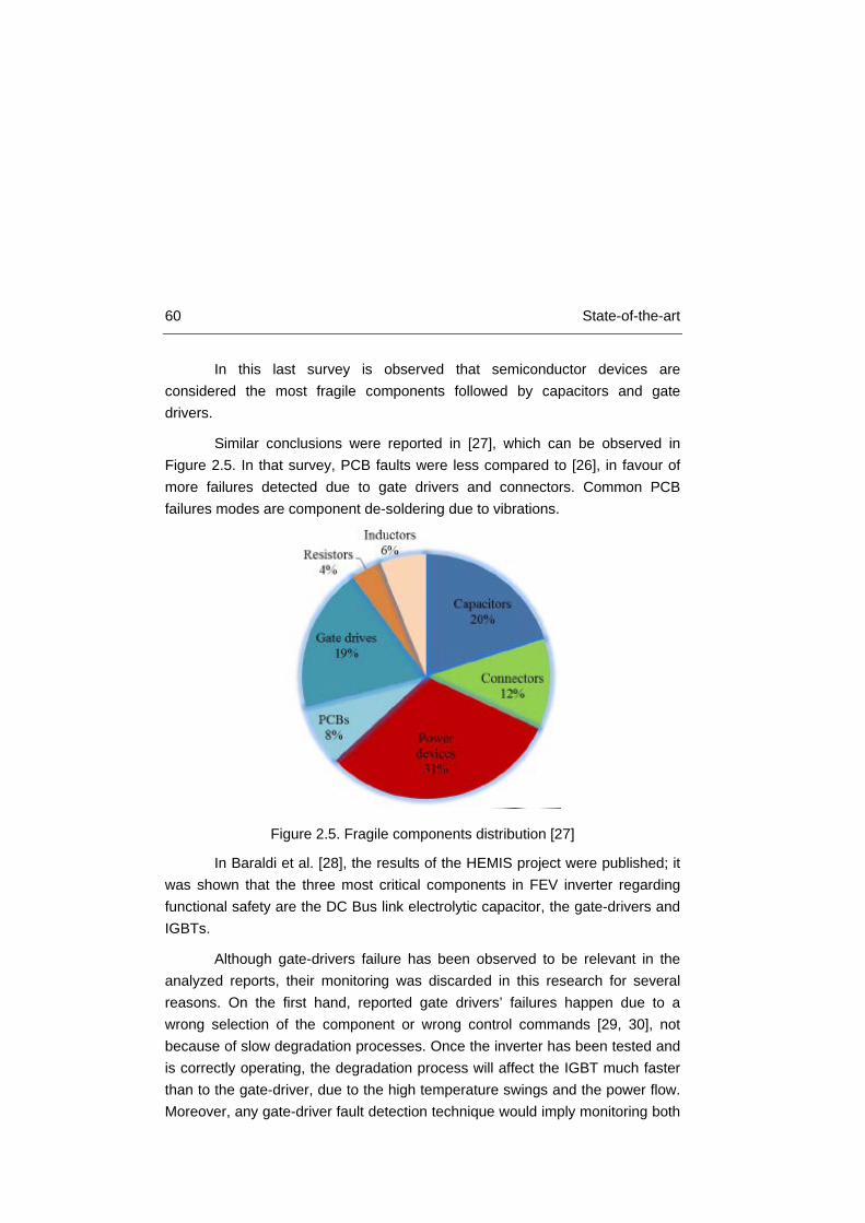
60 State-of-the-art

In this last survey is observed that semiconductor devices are considered the most fragile components followed by capacitors and gate drivers.

Similar conclusions were reported in [27], which can be observed in Figure 2.5. In that survey, PCB faults were less compared to [26], in favour of more failures detected due to gate drivers and connectors. Common PCB failures modes are component de-soldering due to vibrations.

Figure 2.5. Fragile components distribution [27]

In Baraldi et al. [28], the results of the HEMIS project were published; it was shown that the three most critical components in FEV inverter regarding functional safety are the DC Bus link electrolytic capacitor, the gate-drivers and IGBTs.

Although gate-drivers failure has been observed to be relevant in the analyzed reports, their monitoring was discarded in this research for several reasons. On the first hand, reported gate drivers’ failures happen due to a wrong selection of the component or wrong control commands [29, 30], not because of slow degradation processes. Once the inverter has been tested and is correctly operating, the degradation process will affect the IGBT much faster than to the gate-driver, due to the high temperature swings and the power flow. Moreover, any gate-driver fault detection technique would imply monitoring both

Chapter 2 61

the input and the output signals and comparing both of them. This option was not considered interesting from the cost and the intrusiveness points of view, following the suggestions of the IAP.

In addition to the previously mentioned failures, there are some other negative points affecting the reliability of inverters, which are a consequence of the control strategies that are implemented nowadays, i.e. Pulse Width Modulation (PWM). In order to generate the AC voltage, the inverter usually works in a “hard switching” mode. In this mode, the inverter switches the semiconductor devices at high speed, involving high voltage slew rates (dv/dt) and high common mode voltages [31]. This situation causes problems such as electromagnetic interference, winding failures, ground leakage currents and faster degradation of semiconductors. Three consequences of these problems are presented:

• Device Stress: The overlapping of voltage and current waves during each switch-on and switch-off produce some high energy losses, thus an increase in the operating temperature. Consequently, the operating frequency of the inverter must be limited to reduce this effect.

• EMI: It is known that high dv/dt, and high di/dt at the switching of fast devices can produce severe EMI problems that can affect the reliability of nearby systems, such as the control boards.

• Wiring Insulation Degradation: The high dv/dt across the insulation of the stator windings of the traction machine can create large current displacement, which can lead to deterioration of the machine insulation.

The main issues regarding inverter reliability have been reviewed and the employment of a PHMS is justified in order to improve the safety and reliability. A key point for PHMS development, which is demonstrated in the different applications reviewed, is the requirement of acquisition of relevant data showing the degradation process of components in order to develop the monitoring algorithms. Therefore, a review of accelerated aging tests performed in power electronic devices in order to obtain degradation data will be reviewed.

62 State-of-the-art

2.3 Accelerated Aging Tests In the way for PHMS implementation, data belonging to the degradation

process of components is required for different actions, following the needs observed in Chapter 1.

Accelerated aging tests are a common practice for data collection regarding components degradation and lifetime analysis [29, 30, 32]. Accelerated aging tests are a common practice for reliability and durability testing, as well as a quick way to collect operating data. Accelerated aging tests have also been employed as a validation process for new components before hitting the market. They allow the effects of failure modes and mechanisms to be analyzed and failure precursor parameters to be identified. Accelerated aging test development was widely studied by G. Hobbs [33].

The procedure consists on applying stresses well in excess of those that will be seen during the service period. Thus, failures are caused to occur much faster. Typically, the times or cycles to failure in accelerated tests will be several orders of magnitude less than would be observed in service [24]. A metric employed to determine the stress quantity is the acceleration factor AF.

𝐴𝐹 = 𝑡𝑜𝑝𝑡𝑠𝑡𝑟𝑒𝑠𝑠

(Eq. 2.1)

Where, 𝑡𝑠𝑡𝑟𝑒𝑠𝑠 is the operating point set higher than the nominal operating point, 𝑡𝑜𝑝. However, the AF metric is rarely employed, as it assumes a constant degradation rate and it is not useful when variable conditions are tested. The induced physical stresses can be electrical, mechanical or thermal. Typically, high temperatures, large currents, vibrations or even shock tests are developed [24].

In [34], the key features that accelerated aging tests must have are presented:

• The dominant failure mode under normal stress and under accelerated stress should be the same.

• The engineering properties associated with the failure mechanisms of a material under accelerated stress should be the same before and after the test.

Chapter 2 63

• The shape of the failure probability density function for the failure mechanisms at rated and higher stress levels should be the same.

Usually, accelerated aging tests have also been related to stress tests, although they are different. Stress tests would be included in the tests for a new component before making it available to the general public. However, they differ with accelerated aging tests, in that the first looks to drive the component to the limit, but without failing; while the latter seek to know when and how the component will fail under certain circumstances. Stress tests are standardized depending on the industry of application. Electronic components to be embarked within a vehicle follow the standards set by the Automotive Electronics Council. However, there are not specific standards regarding power electronic components testing for electric vehicles yet. As a result, manufacturers are developing their traditional qualifying tests for standard industrial components [24] (i.e. High Temperature Reverse Bias, High Humidity, Thermal Shock, Power and Thermal Cycling).

Given the variety of accelerated aging test developed for both capacitors and IGBTs they are separately reviewed in the next sub-sections. It must be highlighted that a great amount of the relevant literature on the topic has been developed by the CALCE research group with many and varied contributions.

2.3.1 Accelerated Aging Tests on capacitors Aluminum electrolytic capacitor degradation has been investigated by

several authors.

In [35], Kulkarni et al. employed an electrical overstress (EOS) method for studying the degradation effects of electrolytic capacitors subjected to loading under extreme operating conditions. The method consisted on rapidly charging/discharging of capacitors. A square-wave of 200 mHz was employed to charge the capacitors and then, a RC circuit was used for discharging.

Celaya et al. [36], applied separately electrical and thermal overstresses on electrolytic capacitors. In the electrical overstress (EOS) the capacitors were subjected to voltage stresses, similar to the ones developed in [35]. It was observed that the higher the amplitude level of the charge/discharge signal, the

64 State-of-the-art

higher the degradation rate was. During the thermal overstress, high storage temperature conditions were replicated, rising the temperature in an oven to 125 ºC in time steps. Electrolytic capacitors Equivalent Series Resistance (ESR) and Capacitance where measured during the degradation process. The variation of Capacitance due to thermal stress can be observed in Figure 2.6, where capacitance is plotted vs. the aging time.

Now, the variation of the ESR which is plotted vs. the aging time is shown in Figure 2.7 during electrical overstress.

Figure 2.7. ESR and C variation for EOS [36]

Figure 2.6. Capacitance variation for thermal overstress [36]

Chapter 2 65

A great percentage variation of both the capacitance and the ESR are observed. Thus, they could be selected as failure precursor parameters.

In [37], the main degradation mechanisms of a capacitor were analyzed and its equivalent circuit model developed. A degradation model with an exponential trend was suggested following the data provided by the vendor. The accelerated aging tests conditions to which the components were submitted are: ambient temperature 105 ºC, and 1 Arms at 120 Hz. Therefore, a mixture of temperature and electrical overstresses was applied.

2.3.2 Accelerated Aging Tests on IGBTs Accelerated aging tests are a common practice for assessing the

reliability of semiconductor devices [10, 32, 38, 39, 40]. Junction temperature has been described as the main variable affecting and describing the degradation of IGBTs [29, 30]. As a result, most reports suggested increasing its value further than the limits provided by the manufacturer to accelerate the degradation process.

In Hensler et al. [10], and Smet et al. [32], accelerated aging tests were performed on IGBT modules for automotive applications. Electro-thermal aging was considered in both articles, in which the junction temperature was driven to values higher than its maximum nominal value. Different test procedures were applied: DC and PWM signals were applied to the gate and their influence on the degradation process was analyzed. The authors observed changes in the values of collector-emitter on-state voltage (VCE,ON) and thermal resistance (RTH) before IGBT failure. In Patil et al. [38], degradation was induced by considering temperature values well above the nominal, observing over 315 ºC on the case. Changes in component transconductance, collector-emitter on-state voltage and threshold voltage were observed during the degradation process. Celaya et al. [40], developed an accelerated aging system for different types of semiconductors. Since the study was focused on electrical stresses, the accelerated test conditions were attained by electrical operation of the devices at temperatures within the range that was below maximum ratings and above room temperature. This was done by controlling case temperature. Changes in threshold voltage were observed.

66 State-of-the-art

A common practice for product qualifying among manufacturers is power cycling [24]. A power cycling test followed by Infineon Technologies is commuting the component to obtain junction temperature variations of 60 ºC between 2 and 5 sec. However, the maximum junction temperature is never driven above the maximum operating limits; therefore, it would not be a properly called accelerated aging test, although some ideas can be drawn on how the tests could be developed.

Once the reliability of power electronics has been studied and the different approaches to data collection through accelerated aging tests have been presented, we can proceed with the state-of-the-art on how to estimate the RUL of components.

2.4 Prognosis The previous introduction to power electronics reliability and accelerated

aging tests to collect degradation data, allows us to properly move to prognosis, which is the ability to estimate the health of a component. The key point is to answer the following question: what can be done when the requirements of standards are followed when designing an item, but the required safety levels of the item are not met? This could be the case in safety critical applications, where the predicted failure time of a given item is inherently below the objective established by the safety level.

There might be systems that do not fulfill the required safety levels, but need to be embarked. This is the case of certain power electronic devices (i.e. semiconductor devices), which intrinsic manufacturing process leads to very stochastic (time varying) degradation processes, and thus, they are very unreliable. On the other hand, they greatly allow reducing weight and space, which are appreciated benefits. Therefore, several techniques have been proposed traditionally to counteract the effect of low reliability levels of equipment [2, 34]. The most extended are:

• Redundant systems.

• Fault-tolerant design.

• Fault diagnosis.

Chapter 2 67

• Prognosis.

The principle of redundant systems operation is several elements working simultaneously, but they are capable of carrying the ‘load’ themselves if required, such as the engines on civil airliners. Other redundant systems principle consists on having idle elements that ‘awake’ when the system needs them, such as backup generators. Therefore, reliability can be increased by employing redundancy on part or at a system level, without affecting the safety level of the system.

Fault-tolerant design is based on the principle that systems’ most critical failure modes can be identified and addressed specifically. A fault-tolerant device can maintain the system performance in the presence of a component failure. When a part of the device fails, another will take over for a time, until the faulty device is replaced. An example of fault-tolerant electric-machines design is provided by B. Prieto [41]. Upon the criteria that the most common failures in machines are phase short and open circuits, a multi-phase permanent magnet synchronous machine (PMSM) design is suggested. In case one of the phases fails, firstly, it is able to withstand the short-circuit current, and then, the rest of the phases are still able to carry on with the operation of the machine. This design has great impact on the associated power electronics topology and the motor control algorithm. Despite the benefits of fault-tolerant and redundant systems, they increase overall cost, size and weight of the machine, attributes the automotive industry is very concerned about.

Another approach is fault diagnosis [42]. It is based on the capability of assessing the failure of a system, and thus, warning the operator about the situation. A certain kind of intelligence must be placed within the system in order to identify the root source of the failure. An example on the automotive industry is found with On Board Diagnostics (OBD) system. It gathers information related to the operation of the vehicle and provides useful information for repair and maintenance operations. Nevertheless, diagnosis operates once the failure has occurred, negatively influencing on the availability and costs of the system, due to the repair time.

Under the previous considerations, prognosis is understood to be a possible optimum solution. Prognosis is the ability to predict the RUL and the health state of a degrading item. The main advantage compared with the rest of

68 State-of-the-art

the techniques proposed is that prognosis warns in advance of the impending failure. Thus, it is possible to define predictive maintenance policies that allow the optimal exploitation of the useful life of the monitored equipment, with benefits in terms of costs reduction and improvement of safety.

Prognostic systems have received several terms to refer to Prognosis and Health Monitoring (PHM), including Integrated Systems Health Management (ISHM), Integrated Vehicles Health Management (IVHM), Condition-Based Maintenance (CBM), and Health and Usage Monitoring systems (HUMS). Despite the recent emphasis on the field of PHM, health state monitoring for subsystems such as aircraft engines has been part of the engineering practice [43].

Nevertheless, PHM integration has found different implementation approaches, as it has been previously stated in section 2.1. Each of the presented cases had a certain way to implement the prognostic model. In Vichare et al. [44], the different prognostic models are summarized in four:

• Built-In-Test (BIT).

• Use of fuses and canary devices.

• Modeling accumulated damage based on measured life-cycle loads.

• Monitoring and reasoning of failure precursors.

The employment of these different approaches faces challenges and the most appropriate for each application should be selected. Once the potential failure modes, mechanisms, and effects have been identified, a combination of BIT, canaries, precursor reasoning, and life-cycle damage modeling may be necessary, depending on the failure attributes. In fact, different approaches can be implemented based on the same sensory data.

BIT is defined as an on-board hardware-software diagnostic meant to identify and locate faults, which may include error detection and correction circuits, totally self-checking and self-verifying [44]. However, BIT system lacks any information of the operating component itself; therefore, operating component’s lifetime is unknown and the failure is detected once it happens. As the degradation conditions are not fully known in this research, provided the absence of data in a FEV, this approach is discarded.

Chapter 2 69

Another approach is the employment of canary devices. The name comes from the canaries employed in mines to detect the presence of gases. Canary devices mounted on the product have been used to provide advanced warning of failure due to specific wear out failure mechanisms. Mishra et al. [45], studied the applicability of semiconductor-level health monitors by using pre-calibrated cells (circuits) located on the same chip of the actual circuitry. It was aforementioned the example of InstaCell [46], which follows this same strategy. The main disadvantage of this approach is the absence of knowledge of when the failure is going to happen exactly, although the canary provides a prior warning.

The third approach is based on modeling the accumulated damage. The damage accounted during the life-cycle of the item, including: manufacturing, storage, handling, operating and non-operating conditions, is considered. These life-cycle loads may lead to physical degradation of the component, reducing its service life. The aim of these systems is to measure the loads in-situ and in conjunction with damage models to assess the degradation. Ramakrishnan et al. [47] introduced the life consumption monitoring methodology, which combined in-situ measured loads with physics-based stress and damage models for assessing the life consumed. The lack of a test bench in real operational conditions in which to collect the information of the whole life cycle prevents us from applying this prognostic approach.

Finally, the monitoring and reasoning of failure precursor parameters is studied. Failure precursors are physical or operational characteristics of the component directly related to its degradation. For example, a drift from the nominal voltage of a power supply under certain conditions could mean an impending failure of the feedback sensing circuitry. Measuring the precursor parameters and a clever interpretation of the signals, could lead to the detection of the impending failure. If the event of a failure is gradual and follows a certain trend, the trend could be identified, and upon the selection of an appropriate limit threshold, a warning alarm could be provided in order to avoid the failure. This is one of the most common approaches to prognostics in modern systems, mainly due to the advances on non-intrusive sensors, statistical inference and machine learning algorithms, which allow an accurate prediction of the RUL of the components. As it has been introduced in Chapter 1, this last option is the selected choice for the PHM system that will be implemented, provided the

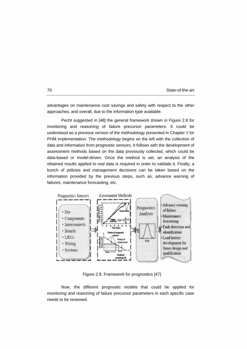
70 State-of-the-art

advantages on maintenance cost savings and safety with respect to the other approaches, and overall, due to the information type available.

Pecht suggested in [48] the general framework shown in Figure 2.8 for monitoring and reasoning of failure precursor parameters. It could be understood as a previous version of the methodology presented in Chapter 1 for PHM implementation. The methodology begins on the left with the collection of data and information from prognostic sensors. It follows with the development of assessment methods based on the data previously collected, which could be data-based or model-driven. Once the method is set, an analysis of the obtained results applied to real data is required in order to validate it. Finally, a bunch of policies and management decisions can be taken based on the information provided by the previous steps, such as, advance warning of failures, maintenance forecasting, etc.

Now, the different prognostic models that could be applied for monitoring and reasoning of failure precursor parameters in each specific case needs to be reviewed.

Figure 2.8. Framework for prognostics [47]

Chapter 2 71

2.4.1 Prognostic models Prognostics of failures in engineered equipment are based on the

capability of predicting future degradation paths, so as to estimate the Remaining Useful Life (RUL) of the equipment [49]. On this basis, it is possible to define predictive maintenance strategies to set the best maintenance actions for allowing the optimal exploitation of the useful life of the monitored equipment, with benefits in terms of reduction of costs and improvement of safety [50].

In practice, industrial equipment works in varying operating conditions. These variations can have remarkable effects on the degradation process and on the values of the signals measured to monitor it [51]. For example, structures operating in environments characterized by high temperatures usually show faster degradation than structures operating at low temperatures, besides high temperatures may modify the measurement of electrical signals used to estimate the degradation of an electrical device. Thus, it is fundamental that prognostic methods properly take into account the effects of variations due to operating conditions [52].

In order to provide useful and reliable predictions, prognostic models need to take into account the different sources of noise or uncertainty when making a prediction. The degradation process of power electronic components has been demonstrated to be affected by several sources of uncertainty [30, 40, 53]. Among them, the stochasticity of the degradation process of semiconductor devices is a major difficulty. Given the characteristics and constraints of the problem, there are many factors influencing the performance of prognostic systems, such as, (i) the dependence of the algorithm’s accuracy on the quantity of valid reference patterns; (ii) the variability associated to manufacturing conditions and uncertainties in environmental and operating conditions; and (iii) the sensory signal relationships with different health states. The prognostic models have to overcome these sources of noise and provide measurements of the uncertainty affecting the RUL predictions.

The implementation of the algorithms for RUL prediction hugely depends on the data type or information available. Consequently, prognostic methods have commonly been splitted depending on the information available. They are splitted in two, data-driven models and physics-based models, which

72 State-of-the-art

we proceed to explain now. Some researches have also employed the so-called hybrid models, which is the combination of data-driven and model-based approaches. A final approach has been suggested as well, which is an ensemble of models. Ensemble of models has been employed in data-driven approaches. It relies on the idea that the combination of different data-driven approaches improves the final result.

2.4.1.1 Data-driven models

Data-driven models are based on statistical or artificial intelligence approaches, such as Artificial Neural Networks (ANN) [54], Autoregressive Moving Average techniques [55] and Relevance Vector Machines [56] that ‘learn’ trends from collected data [57]. Wang and Vachtsevanos proposed architecture for prognosis employed dynamic wavelet neural networks (DWNN), reinforcement learning and genetic algorithms [57]. Most popular data-driven approaches to prognostics are Artificial Neural Networks (ANN). Although, decision trees, Support Vector Machines (SVM), wavelets, regression, statistical methods and fuzzy logic have been reported as well [57].

2.4.1.2 Physics-based models

Model-based prognostic approaches use an explicit physics-based model of the degradation process to assess the current degradation state and to predict its future evolution. This is, mathematical representations of the equipment degradation process are employed to predict the equipment RUL However, in several prognostic applications the degradation state of the system is not directly observable and measurements can be affected by noise. Thus, many approaches rely on Bayesian methods that iteratively assess the component degradation state [58]. Examples belonging to the latter are the exact and extended Kalman Filters (KF). Recently, numerical approximations based on the use of Monte Carlo sampling techniques, such as Particle Filtering, have gained popularity for their ability to deal with non-linear degradation models and non-Gaussian noises [58].

In model-based prognostics, it is possible to distinguish between two different situations: i) the effects of operating conditions on the degradation process and on the measured signals are known and represented in the mathematical models, ii) the effects are not fully known and a mathematical

Chapter 2 73

model of the operating conditions influence is not available. In the former situation i), traditional model-based prognostic approaches, such as those based on Bayesian Filters [59], can be directly used, whereas in the latter one ii) tailored prognostic approaches need to be developed.

2.5 Prognosis of Capacitors Although prognostic model examples applied in FEVs are not available,

the research developed in discrete components on the prognosis field is wide. In this sense, the researches developed on capacitors prognosis are reviewed now.

In this work we face the problem of predicting the RUL of aluminum electrolytic capacitors installed in Fully Electric Vehicles (FEVs) [52]. The main task of this component, which is the most commonly used in the electronics industry [60], is to filter the rail voltage provided to the inverter of the electric motor [61]. According to [27], electrolytic capacitors are very critical components, being responsible for almost 30% of the total number of failures in electrical systems and, thus, it is of paramount importance to develop predictive maintenance approaches for them, as we saw in Chapter 2.2.

The failure mechanisms of the aluminum electrolytic capacitors can be catastrophic or gradual. In case of catastrophic failures, capacitors completely and abruptly lose its function due to short or open circuits, whereas gradual failures are characterized by a gradual functionality loss [62, 63, 64]. Similarly to gate drivers’ case, catastrophic failures are related to a wrong selection of components or poor testing prior to final deployment. The main cause of gradual degradation mechanism, which is the most common in electrolytic capacitors, is the vaporization of electrolyte (see Chapter 3). This degradation process is strongly influenced by the capacitor operating conditions, such as voltage, current, frequency, and working temperature [35]. In capacitors installed in FEVs, these conditions would tend to continuously change due to external factors such as season, geographical area and driving style. In particular, the temperature experienced by the capacitor, which depends on the applied loads and on the ambient temperature, has a remarkable influence on the evolution of the degradation process: higher the temperature, faster the vaporization process due to the increase of the self-heating effects [65].

74 State-of-the-art

Aluminum electrolytic capacitor degradation has been investigated by several authors. A direct degradation indicator for capacitors operating at constant temperature and load is the Equivalent Series Resistance (ESR) [37, 66, 67, 68]. A capacitor is considered failed, i.e. not able to properly accomplish to its functions, when its ESR exceeds the double of its initial value [69]. In [37], the main degradation mechanisms of a capacitor were analyzed and its equivalent circuit model developed.

In [66], a degradation model based on the physics of the wear-out mechanism was presented. In [70], a method based on the use of genetic algorithm for the identification of the parameters of the degradation model was discussed. In [35], a method for studying the degradation effects of electrolytic capacitors subjected to loading under extreme operating conditions was proposed. Furthermore, some approaches for monitoring capacitor degradation and for predicting its RUL were proposed. In [71], a method for real-time monitoring and RUL prediction for electrolytic capacitor used in uninterruptible power supplies (UPSs) was developed.

However, the temperature at which the ESR measurement is performed has a remarkable influence on the observed ESR value (higher the temperature, lower the ESR). Moreover, the models mentioned above consider capacitors aging at constant temperature and do not quantify the uncertainty on their predictions. A Bayesian approach for the prediction of the capacitor RUL probability distribution has been proposed in [61], where a prognostic methodology based on the application of a KF for tracking the capacitor health state, forecasting the capacitance evolution and predicting the capacitor RUL was presented. This approach does not consider the possibility of variable operating and environmental conditions and, as underlined by the authors themselves, it is not able to cope with the abrupt change of the capacitor functional behavior arising near the end of the component life, thus providing inaccurate RUL predictions.

2.6 Prognosis of IGBTs The degradation process of IGBTs has been demonstrated to be

affected by several sources of uncertainty [30, 40, 53]. Two failure types are reported for IGBTs: sudden and progressive. Sudden failures could be

Chapter 2 75

addressed through diagnostic approaches, but their prediction through prognostic rules is a most difficult task and for this reason they are typically disregarded in prognostic studies [30, 72, 73]. Therefore, they are left out of the scope of this work. Lifetime estimations consider that sudden failures have a constant occurrence probability during the lifetime of the component.

With respect to progressive failures, the understanding and analysis of IGBT degradation mechanisms have advanced. According to [30, 32, 39, 53], the parameter more influencing the degradation process is the junction temperature variation. Thus, a great number of the reviewed researches try to measure or get a precise approach of the junction temperature [29, 30]; however, they are not prognostic approaches.

In this section, we review the methods proposed for modeling the IGBT degradation process and predicting IGBT RUL. The first three subsections are devoted to the discussion of i) physics-based models ii) data-driven models, and iii) ensemble models, and a fourth subsection presents a summary of the conclusions drawn from the literature review.

2.6.1 Physics-based models for IGBT prognosis Celaya et al. [40], exploit the on-state resistance exponential variation

model to assess the degradation state of MOSFETs through the application of a KF. Lifetime modeling techniques are applied in order to predict the fatigue life of wire bonds and solder joints of IGBTs under cyclic loading conditions [29]. The LESIT project equation, which relies on the Arrhenius law, has been used to predict IGBT lifetime in several works [30, 74]. Denk et al. [75], proposed a method for measuring the junction temperature online, which, when combined with the equation from Bayerer et al. [53], provided lifetime predictions.

The results of power cycling tests were employed by Huang and Mawby to fit a degradation model based on the Coffin-Mason law and on the assumption that solder joint fatigue was the dominant IGBT failure mechanism [29, 38]. The approach applied the rainflow counting algorithm developed by Matsuishi and Endo [76] to take into account the average and the swing values of the junction temperature. Then, Miner’s rule, which assumes linear damage accumulation, was applied to assess IGBT degradation.

76 State-of-the-art

𝐷𝑎𝑚𝑎𝑔𝑒 = ∑ 𝑁𝑖𝑁𝑓𝑖

𝑛𝑖=1 (Eq. 2.2)

where, Ni is the number of cycles at a stress level i, and Nfi represents the number of cycles to failure at that particular stress level. It is assumed that the damage is complete when Damage = 1.

A physics-based model was developed as part of the LESIT project [74], which has been largely employed by different researches. It provides the number of cycles to failure at a particular stress level, given by the average (TJ,med) and swing (∆TJ) junction temperature.

𝑁𝑓𝑖 = 𝐴∆𝑇𝐽𝛼𝑒( 𝑄𝑅∗𝑇𝐽,𝑚𝑒𝑑

) (Eq. 2.3)

Where, A = 640 and α = -5 are constants, Q = 7.8 ∗ 1014 J/mol and R is the gas constant. This model, based on the Arrhenius law, has been adopted since experimental tests suggest that IGBT degradation is mainly caused by thermally activated creeping processes. Furthermore, the model is able to cope with junction temperatures above the nominal temperature such as those encountered in accelerated aging tests.

Bayerer et al. [53] proposed a more refined model for assessing the number of cycles (Nfi) taking into account other parameters that influence the degradation process, such as the power on time or the current per wire. It also takes into account the results of a large campaign of experimental tests on IGBTs. This model only applies to IGBTs working with a junction temperature in the range 50 to 150 ºC. This constraint comes from the statistical treatment of the vast amount of data employed to obtain the value of the parameters of the model. As a result, the equation is not valid outside the boundaries of the fitted data. Thus, the value of the β parameters in Eq. 2.4 was set, and therefore the variation of the curve was restricted.

𝑁𝑓𝑖 = 𝐾∆𝑇𝐽𝛽1𝑒

𝛽2𝑇𝐽+273𝑡𝑜𝑛

𝛽3𝐼𝛽4𝑉𝛽5𝐷𝛽6 (Eq. 2.4)

Where, K is a constant, ∆TJ is the junction temperature variation, ton is the power on time, I is the current per wire, V is the breakdown voltage which is related to the chip thickness and D is the diameter of the bonding wires.

Chapter 2 77

2.6.2 Data-driven models for IGBT prognosis Given the lack of sufficient public data collected during the degradation

of IGBTs, examples of applications of data-driven approaches to IGBT degradation modeling and IGBT RUL prediction are scarce. In Rigamonti et al. [77] a Self-Organizing Map (SOM) was tested on healthy and degraded IGBTs working in an electric inverter. The algorithm was able to assess IGBT degradation level, but it did not provide a RUL prediction. In Celaya et al [78], Mahalanobis Distance (MD) was computed and when an anomaly was detected, a particle filtering algorithm based on a polynomial regression of data was triggered to predict the RUL of MOSFETs. This approach showed limitations to obtain good results, since it applied a specific polynomial curve that not all the components degradation patterns followed.

2.6.3 Ensemble methods for IGBT prognosis The idea behind the use of an ensemble of models is that the

combination of several model outcomes provides better performance than what a single model does. Ensemble of models is commonly employed for data-driven models.

Different techniques for aggregating the outcomes of individual models into an ensemble outcome were investigated in [79], moving from algebraic combination rules (majority voting, max/min, average [80]) to fuzzy integral combination, Dempster-Shafer based fusion and bagging and boosting predictors. In Tamilselvan et al. [81], the aggregation of the degradation states provided by an ensemble of classifiers was performed by resorting to a weighted majority voting with dominance. In practice, the aggregation is guided by the local performance of each model. These methods rely on the idea that each model can perform well in some regions of the input space and poorly in others.

In Baraldi et al. [48], a hybrid prognostic methodology was proposed in which a degradation dataset was available but a physical model was missing. It was suggested that a dataset could be used to train a bootstrapped ensemble of Artificial Neural Networks (ANN), which was then embedded in a Particle Filtering algorithm as an empirical measurement model.

78 State-of-the-art

2.7 Conclusions about the state-of-the-art The main conclusions extracted from the review of the state-of-the-art

on the different topics are presented. Then, the contributions of the present research to that state-of-the-art are exposed.

2.7.1 Conclusions about PHM implementations It is concluded that PHM implementations are very new and are mostly

employed on safety critical applications, such as aerospace and military industries. The architecture and implementation of the systems widely vary from one application to another. However, no applications in the automotive industry have been found, although interest on them is high following the number of patents published.

As a result, the proposed PHMS is designed to be applied to the FEV powertrain electronics.

2.7.2 Conclusions about Power Electronics Reliability The employment of power electronic converters on FEVs was reviewed.

The converter with higher power requirements and demanding operating conditions is the inverter driving the electric motor. The absence of failure statistics and studies on real data collected on a FEV powertrain forced to analyze the results on industrial applications. Capacitors and power semiconductor devices were pointed as the main failure causes. Other components such as PCBs and gate drivers were also pointed as important possible failure causes. However, monitoring of these components was discarded in a first stage due to different issues with the selected PHM features. Consequently, the ongoing studies are focused on electrolytic capacitors and power semiconductor devices.

2.7.3 Conclusions about Accelerated Aging tests It is concluded that several researches have obtained data through the

development of accelerated aging tests. Different methodologies have been observed depending on the component type. The researches have stated

Chapter 2 79

different degradation mechanisms and failure precursor parameters for both IGBT and capacitor technologies. Nevertheless, a deep review on the reported degradation mechanisms on both components is required, in order to select appropriate failure precursors and a good understanding of the physics behind the degradation. On the other hand, the development of accelerated aging tests for both components is an unavoidable duty in order to obtain data from the degradation process.

Regarding the degradation modes and mechanisms of capacitors, they have been studied and analyzed in previous researches. However, the accelerated aging tests have helped to confirm them and to validate the prognostic algorithm development with the collected data.

Regarding the degradation mechanisms of IGBTs, it has been observed that there is controversy on the most important one. It has also been observed that tests have been developed on both new and old IGBT technologies, but the results have never been compared. As a consequence, accelerated aging tests have been developed and a deep analysis of the root causes underlying component degradation is done. The accelerated aging tests are employed to identify the failure precursor parameters. They were carried out on different IGBT technologies to evaluate the applicability of the prognostic model.

2.7.4 Conclusions about Prognosis in Capacitors Regarding the literature review done on prognosis of electrolytic

capacitors, several conclusions can be extracted. To begin with, there are several points that previous researches are missing:

• They assume constant degradation temperatures. Therefore, the estimation of the lifetime of capacitors working on variable operating conditions, such as a FEV powertrain, would not be possible.

• The effect of temperature on ESR measurements is not considered.

• The predictions are not supplied with any uncertainty boundary.

Nevertheless, a major achievement of these researches is the development of useful mathematical models of the degradation process, as well as the identification of the main failure mechanisms. Taking into account the

80 State-of-the-art

previous conclusions, the contributions of the present work beyond the state-of-the-art will be presented. The objective of the present work will be to provide a method for the prediction of the RUL for a capacitor working in variable operating conditions, which ESR can be measured at different temperatures. The method will also be able to estimate the uncertainty affecting the RUL prediction.

In order to give an answer to the previous objectives, a sequential Bayesian approach for the estimation of component degradation will be employed. The Bayesian approach is able to account for the uncertainty affecting: i) the ESR and temperature measurement process, ii) the possible inaccuracy of the degradation model, iii) the stochasticity of the degradation process. In this type of problems, KF have been applied, however, due to the presence of non-additive (non-Gaussian) noise terms, a Particle Filtering (PF) approach will be implemented. PF allows to properly take into account the uncertainty on the present degradation state estimation and the uncertainty on the future evolution of the operating conditions.

To the best of the author’s knowledge, the implementation and application of a PF approach for RUL uncertainty estimation has not been yet considered for electrolytic capacitors.

2.7.5 Conclusions about Prognosis in IGBTs Several conclusions can be extracted from the review done. The

techniques present in the literature are few and still have difficulty assessing the RUL of IGBTs accurately. On the one hand, physical degradation models are not capable of adapting to the characteristics of each particular component. On the other hand, data-driven models are not able to accurately predict RUL in the long run, mainly because of the minute variation in the degradation estimation precursor parameters [32], which usually change rapidly in the end-of-life of the component. Thus, for long periods of time little information regarding the health state is available. Such models also have to overcome the lack of databases on IGBT degradation, and thus it is difficult to generalize data-driven models.

Another issue observed regarding IGBT RUL prediction is that they do not provide uncertainty boundaries of the predictions.

Chapter 2 81

Taking into account the previous conclusions, the contributions of this work beyond the state-of-the-art are presented. In this work, we consider the benefits of gathering both sources of information, data-driven and physics-based models, with specific reference to the problem of predicting the RUL of IGBTs installed in FEVs [10].

Given the characteristics and constraints of the problem, a single data-driven or model-based approach is not expected to meet performance requirements. Thus, we have developed an ensemble approach which leverages the strengths of different algorithms to form a robust unified algorithm [81].

The three main novelties of the proposed prognostic method are:

• The employment of a bootstrapped aggregation ensemble for directly estimating the RUL of IGBTs together with RUL estimation uncertainty.

• The application and validation of the method with real experimental data from three different IGBT types.

• From the methodology point of view, the input to the prognostic model of a mixture of data-driven and physics-based model information for IGBT monitoring.

To the best of the author’s knowledge, a hybrid ensemble based on the use of both physics-based and data-driven models has not been yet considered for predicting IGBT RUL.

Following the results of the review on Section 2.7.3., the next Chapter will proceed with a deep analysis of the failure modes and mechanisms as well as failure precursor parameters of electrolytic capacitors and IGBTs, before the explanation of accelerated aging tests.

82 State-of-the-art

2.8 References [1] “IEEE Standard Framework for Reliability Prediction of Hardware," in IEEE

Std 1413-2010 (Revision of IEEE Std 1413-1998), pp.1-20, April 9, 2010

[2] P.D.T. O’Connor, “Practical Reliability Engineering,” Wiley Online Library, 4th Edition, 2004, ISBN: 0-470-84463-9

[3] M. J. Cushing, D.E. Mortin, T.J. Stadterman, and A. Malhotra, “Comparison of Electronics-Reliability Assessment Approaches,” in Reliability, IEEE Transactions on, vol. 42, no. 4, pp. 542-546, 1993

[4] “IEEE Guide for Selecting and Using Reliability Predictions Based on IEEE 1413," in IEEE Std 1413.1-2002, pp. 0-1, 2003

[5] J.J. Fox and B.J. Glass. “Impact of integrated vehicle health management (IVHM) technologies on ground operations for reusable launch vehicles (RLVs) and spacecraft,” Aerospace Conference Proceedings, 2000 IEEE, 2000

[6] M. Schwabacher, J. Samuels and L. Brownston. “NASA integrated vehicle health management technology experiment for X-37,” AeroSense 2002, 2002

[7] A. Halfpenny and S. Kellett, “pHUMS- Prognostic Health and Usage Monitoring of Military Land Systems,” Proceedings of the 6th Australasian Congress on Applied Mechanics, Perth, pp. 1158-1166, 2010

[8] InstaCell Diagnostic/Prognostic IP Library, Ridgetop Group, Inc., January 30, 2002

[9] S. Mishra and M. Pecht, “Remaining Life Prediction of Electronic Products using Life Consumption Monitoring Approach,” European Microelectronics Packaging and Interconnection Symposium, Poland, June 2002

[10] A. Hensler, J. Lutz, M. Thoben and K. Guth, "First power cycling results of improved packaging technologies for hybrid electrical vehicle applications," Integrated Power Electronics Systems (CIPS), 2010 6th International Conference on, pp. 1, 2010

[11] Patent US 6330499, Chou et al. “System and method for vehicle diagnostics and health monitoring,” Assignee: IBM, 2001

Chapter 2 83

[12] Patent US 6609051, Fietcher et al, “Method and System for condition monitoring of vehicles,” Assignee: Daimler Chrysler AG, 2003

[13] Patent US 7260501, Pattipatti et al.,”Intelligent model-based diagnostics for system monitoring, diagnosis, and maintenance,” Assignee: Univ. of Connecticut, Toyota Technical Center, 2007

[14] Patent US 7558655, Garg et al., “Prognostic method and system for hybrid and electric vehicle components,” Assignee: Ford Global Technologies, 2009

[15] Patent US 8095261, Howell et al., “Aggregated Information fusion for enhanced diagnostics, prognostics and maintenance practices of vehicles,” Assignee: GM Global Technology Operations, 2012

[16] Patent US 0336869, Bou-Ghannam et al., “Automotive Predictive maintenance for automobiles,” Assignee: IBM, 2014

[17] J.S. Krupa, D.M. Rizzo, M.J. Eppstein, D.B. Lanute, D.E. Gaalema, K. Lakkaraju and C.E. Warrender, “Analysis of a consumer survey on plug-in hybrid electric vehicles,” Transportation Research Part A: Policy and Practice, vol. 64, pp. 14-31, 2014

[18] C.C. Chan, “The State of the art of Electric Vehicles,” Proceedings of the IEEE, Vol. 95, No. 4, April 2007

[19] G. Wu, X. Zhang, Z. Dong; “Powertain architectures of electrified vehicles: Review, classification and comparison,” Journal of the Franklin Institute, vol. 352, pp. 425-448, 2014

[20] K. Rajasherkara, “Present Status and Future Trends in Electric Vehicle Propulsion Technologies,” Emerging and Selected Topics in Power Electronics ,IEEE Journal of, vol. 1, no. 1, march 2013

[21] B. Ji, “In-situ Health Monitoring of IGBT,” PhD Thesis, Newcastle University, 2011

[22] M. Guarnieri, "Looking back to electric cars," Proceedings HISTELCON 2012, IEEE History of Electro - Technology Conference: The Origins of Electrotechnologies, 2012

[23] K. Rajashekara, “History of electric vehicles in general motors,” Industrial Application, IEEE Transactions on. Vol. 30, no. 4, pp. 897-904, 1994

84 State-of-the-art

[24] A. Volke, M. Hornkamp; “IGBT Modules. Technologies, Driver and Application,” Infineon Technologies AG, Munich, 2nd Edition, 2015

[25] J. de Santiago, H. Bernhoff, B. Ekergard, S. Eriksson, S. Ferhatovic, R. Waters and M. Leijon; “Electrical Motor Drivelines in Commercial All-Electric Vehicles: A Review,” Vehicular Technology, IEEE Transactions on, Vol. 61, no. 2, 2012

[26] S. Yang, A. Bryant, P. Mawby, D. Xiang, L. Ran and P. Tavner, “An industry-based survey of reliability in power electronic converters,” Proceedings of IEEE Energy Conversion Congress and Exposition (ECCE), pp. 3151–3157, Sept.2009

[27] E. Wolfgang, “Examples for failures in power electronics systems,” ECPE Tutorial on Reliability of Power Electronic Systems, April 2007

[28] P. Baraldi, F. Di Maio, M. Rigamonti, E. Zio, A. Galarza, D. Astigarraga, I. Unanue, A. Ruddle and S. Rantala;, "A procedure for practical prognostics and health monitoring of fully electric vehicles for enhanced safety and reliability," Hybrid and Electric Vehicles Conference (HEVC 2014), 5th IET, pp. 1, 2014

[29] H. Oh, B. Han, P. McCluskey, C. Han, B.D. Youn, "Physics-of-Failure, Condition Monitoring and Prognostics of Insulated Gate Bipolar Transistor Modules: A Review,” in Power Electronics, IEEE Transactions on, vol. 30, pp. 2413-2426, 2015

[30] S. Yang, D. Xiang, A. Bryant, P. Mawby, L. Ran, and P. Tavner, "Condition monitoring for device reliability in power electronic converters: a review," in Power Electronics, IEEE Transactions on, vol. 25, no. 11, pp. 2734-2752, 2010

[31] N. Patil, “Prognostics of Insulated Gate Bipolar Transistors,” PhD Thesis, University of Maryland, 2011

[32] V. Smet, F. Forest, J. Huselstein, F. Richardeau, Z. Khatir, S. Lefebvre and M. Berkani;, "Ageing and Failure Modes of IGBT Modules in High-Temperature Power Cycling,” in Industrial Electronics, IEEE Transactions on, vol. 58, no. 10, pp. 4931-4941, 2011

Chapter 2 85

[33] G. Hobbs, “Accelerated Relaibility Engineering: HALT and HASS,” Wiley Online Library, 2001

[34] M. Pecht, “Product Reliability, Maintainability, and Supportability Handbook,” CRC Press, ARINC Research Corporation, 1995, ISBN: 0-8493-9457-0

[35] C. Kulkarni, G. Biswas, X. Koutsoukos, J. Celaya, K. Goebel, ”Integrated diagnostic/prognostic experimental setup for capacitor degradation and health monitoring,” IEEE AUTOTESTCON 2010, 2010

[36] J.R. Celaya, C. Kulkarni, S. Saha, G. Biswas, and K. Goebel; "Accelerated aging in electrolytic capacitors for prognostics," Reliability and Maintainability Symposium (RAMS), 2012 Proceedings - Annual, pp. 1. 2012

[37] M. Hao, and L. Wang, “Fault diagnosis and failure prediction of aluminum electrolytic capacitors in power electronic converters,” Industrial Electronics Society, IECON 2005, 31st Annual Conference of IEEE, pp. 6., 2005

[38] N. Patil, J. Celaya, D. Das, K. Goebel, M. Pecht, "Precursor Parameter Identification for Insulated Gate Bipolar Transistor (IGBT) Prognostics," in Reliability, IEEE Transactions on , vol.58, no.2, pp.271-276, June 2009

[39] R. Amro, J. Lutz, J. Rudzki, R. Sittig and M. Thoben, "Power Cycling at High Temperature Swings of Modules with Low Temperature Joining Technique," Power Semiconductor Devices and IC's, 2006. ISPSD 2006. IEEE International Symposium on, pp. 1, 2006

[40] J. Celaya, P. Wysocki, V. Vashchenko, S. Saha and K. Goebel;, "Accelerated aging system for prognostics of power semiconductor devices," IEEE AUTOTESTCON 2010, pp. 1, 2010

[41] B. Prieto, “Design and Analysis of Fractional-Slot Concentrated-Winding Multiphase Fault-Tolerant Permanent Magnet Synchronous Machines,” PhD Thesis, University of Navarra, 2015

[42] I. Albizu, I. Zamora, A.J. Mazon, A. Tapia; “Techniques for Online Diagnosis of Stator Shorted Turns in Induction Motors,” in Electric Power Components and Systems, vol. 34, pp. 97-114, 2005

86 State-of-the-art

[43] S.B. Johnson, T. Gornley, S. Kessler, C. Mott, A. Patterson-Hine, K. Reichard and P. Scandura, “System Health Management with Aerospace Applications,” Wiley Online Library, 2011, ISBN: 978-0-470-74133-7

[44] N.M. Vichare, M. Pecht, "Prognostics and health management of electronics," Components and Packaging Technologies, IEEE Transactions on, vol.29, no.1, pp.222-229, March 2006

[45] S. Mishra and M. Pecht, “In-situ sensors for product reliability monitoring,” in Proc. SPIE, vol. 4755, pp. 10–19, 2002

[46] I. K Jennions, “Integrated vehicle health management: perspectives on an emerging field,” Training, vol. 2009, pp. 9-12. 2011

[47] A. Ramakrishnan and M. Pecht, “A life consumption monitoring methodology for electronic systems,” in Components and Packaging Technologies, IEEE Transactions on, vol. 26, no. 3, pp. 625–634, Sep. 2003

[48] P. Baraldi; M. Compare; S. Sauco; E. Zio;, “Ensemble neural network-based particle filtering for prognostics,” Mechanical Systems and Signal Processing, Volume 41, Issues 1–2, Pages 288-300, ISSN 0888-3270, Dec. 2013

[49] E. Zio, “Prognostics and health management of industrial equipment,” Diagnostics and Prognostics of Engineering Systems: Methods and Techniques. 2012

[50] J.H. Sheppard and T.J. Wilmering; “IEEE Standards for Prognostics,” IEEE A&E Systems Magazine, 2009

[51] E. Zio and G. Peloni, “Particle filtering prognostic estimation of the remaining useful life of nonlinear components,” Reliability Engineering & System Safety, 2011

[52] B. Ji, V. Pickert, W. Cao, B. Zahawi, “In situ diagnostics and prognostics of wire bonding faults in IGBT modules for electric vehicle drives,” in Power Electronics, IEEE Transactions on, vol. 28, pp. 5568-5577, 2013

[53] R. Bayerer, T. Herrmann, T. Licht, J. Lutz and M. Feller, "Model for Power Cycling lifetime of IGBT Modules: various factors influencing lifetime," Integrated Power Systems (CIPS), 2008 5th International Conference on VDE, pp. 1, 2008

Chapter 2 87

[54] P. Baraldi; F. Cadini; F. Mangili and E. Zio, “Model-based and data-driven prognostics under different available information,” Probabilistic Engineering Mechanics, Elsevier, vol. 32, pp.66-79, 2013

[55] B. Saha; K. Goebel; J. Christophersen;, “Comparison of Pronostic Algorithms for Estimating Remaining Useful Life of Batteries,” Transactions of the Institute of Measurement and Control, vol. 31, pp. 293-308, 2009

[56] K. Goebel, B. Saha and A. Saxena, “A Comparison of Three Data-Driven Algorithms for Prognostics,” in 62nd meeting of the society for machinery failure prevention technology (MFPT) , pp. 119-131, 2008

[57] M. A. Schwabacher;, “A Survey of Data-Driven Prognostics,” in Proceedings of the AIAA Infotech@ Aerospace Conference. 2005. pp. 1-5, 2005

[58] Rigamonti, M.; Baraldi, P.; Zio, E.; Astigarraga, D.; Galarza, A., "Particle Filter-Based Prognostics for an Electrolytic Capacitor Working in Variable Operating Conditions," in Power Electronics, IEEE Transactions on , vol.31, no.2, pp.1567-1575, Feb. 2016

[59] A. Doucet, “On sequential Monte Carlo methods for Bayesian filtering,” Dept. Eng., Univ. Cambridge, UK, Technical Report, 1998.

[60] A. Shrivastava, M.H. Azarian, C. Morillo, B. Sood and M. Pecht,” Detection and reliability risks of counterfeit electrolytic capacitors,” in Reliability, IEEE Transactions on, vol. 63, pp. 468-479, 2014

[61] Celaya, J.R., Kulkarni, C., Saha, S., Biswas, G. & Goebel, K.; "Accelerated aging in electrolytic capacitors for prognostics," Reliability and Maintainability Symposium (RAMS), 2012 Proceedings - Annual, pp. 1. 2012

[62] K. Harada, A. Katsuki and M. Fujiwara, “Use of ESR for deterioration diagnosis of electrolytic capacitors,” in Power Electronics, IEEE Transactions on, vol. 8, no. 4, pp. 355–361, 1993

[63] M.L. Gasperi,; “Life prediction model for aluminum electrolytic capacitors,” Conference Record - IAS Annual Meeting, IEEE Industry Applications Society, vol. 3, pp. 1347-1351, 1996

[64] B. Alvsten,; “Electrolytic capacitors theory and application,” RIFA Electrolytic Capacitors, Sweden, 1995

88 State-of-the-art

[65] A. Lahyani, P. Venet, G. Grellet and P.J.Viverge, “Failure prediction of electrolytic capacitors during operation of a switch-mode power supply,” in Power Electronics, IEEE Transactions on, vol. 13, pp. 1199-1207, 1998

[66] M.L. Gasperi, “Life prediction model for aluminum electrolytic capacitors,” Conference Record - IAS Annual Meeting, IEEE Industry Applications Society, pp. 1347-1351, 1996

[67] A. Braham, A. Lahyani, P. Venet, and N. Rejeb, “Recent developments in fault detection and power loss estimation of electrolytic capacitors,” in Power Electronics, IEEE Transactions on, vol. 25, pp. 33-43., 2010

[68] M.A. Vogelsberger, T. Wiesinger and H. Ertl, “Life-cycle monitoring and voltage-managing unit for DC-link electrolytic capacitors in PWM converters,” in Power Electronics, IEEE Transactions on, vol. 26, pp. 493-503, 2011

[69] P. Venet, H. Darnand, and G. Grellet, “Detection of faults of filter capacitors in a converter,” Application to predictive maintenance, in Proceedings International Telecommunication Energy Conference, pp. 229–234, 1993

[70] F. Perisse, P. Venet, G. Rojat, and J.M. Rétif, “Simple model of an electrolytic capacitor taking into account the temperature and aging time,” Electrical Engineering, vol. 88, pp. 89-95, 2006

[71] K. Abdennadher, P. Venet, G. Rojat, J.M. Rétif and C. Rosset, “A real-time predictive-maintenance system of aluminum electrolytic capacitors used in uninterrupted power supplies,” in Industry Applications, IEEE Transactions on, vol. 46, pp. 1644-1652, 2010

[72] M. Pecht, “Prognostics and health management of electronics,” Wiley Online Library, 2008

[73] J. Gu, N. Vichare, T. Tracy and M. Pecht,; “Prognostics implementation Methods for Electronics,” in Reliability and Maintainability Symposium (RAMS), 2007 Proceedings Annual, pp. 101-106, 2007

[74] M. Held, P. Jacob, G. Nicoletti, P. Scacco and M.H. Poech, "Fast power cycling test of IGBT modules in traction application," in Power Electronics and Drive Systems, 1997. Proceedings, 1997 International Conference on, vol.1, pp.425-430, 26-29, May 1997

Chapter 2 89

[75] M. Kanechika, T. Uesugi, and T. Kachi “Advanced SiC and GaN power electronics for automotive systems,” in Proceedings IEEE International Electronic Devices Meeting, pp. 1-4, Dec. 2010

[76] M. Matsuishi and T. Endo, “Fatigue of metals subjected to varying stress,” Japan Society of Mechanical Engineers, Fukuoka, Japan, 37-40, Mar. 1968

[77] M. Rigamonti, P. Baraldi, E. Zio, A. Alessi, D. Astigarraga, A. Galarza, "A Self-Organizing Map-Based Monitoring System for Insulated Gate Bipolar Transistors Operating in Fully Electric Vehicle," Annual Conference of the Prognostic and Health Management Society 2015, vol. 6, 2015

[78] J. Celaya, A. Saxena, S. Kulkarni, S. Saha, K. Goebel, “Prognostics approach for power MOSFET under thermal-stress aging,” in Reliability and Maintainability Symposium (RAMS), 2012 Proceedings Annual, pp. 1-6, 2012

[79] R. Polikar, "Ensemble based systems in decision making," in Circuits and Systems Magazine, IEEE, vol.6, no.3, pp.21-45, 2006

[80] P. Baraldi, E. Zio, G. Gola, D. Roverso and M. Hoffmann, “Aggregation of Randomized Model Ensemble Outcomes for Reconstructing Nuclear Signals from Faulty Sensors,” In Proceedings of ESREL Conference, vol. 1, pp. 83-88, 2009

[81] P. Tamilselvan, P. Wang, M. Pecht, "A multi-attribute classification fusion system for insulated gate bipolar transistor diagnostics," Microelectronics Reliability, vol. 53, no. 8, pp. 1117-1129, 2013

Chapter 3 91

Chapter 3

3 Failure modes & Failure

Precursor Parameters

In the previous Chapter, the state-of-the-art was presented and conclusions were extracted from it. Among them, the necessity to further analyze and understand the physics and the failure modes of components was claimed prior to the development of accelerated aging tests. In this Chapter, the failure modes and failure precursor parameters of Capacitors and IGBTs will be deeply reviewed.

It is recalled that failure precursor parameters are physical characteristics or variables directly related to the degradation process of components. Their identification will allow determining the RUL of components, which is the final objective of the PHM system. Consequently, a deep understanding of the physics underlying the components behavior is required and will be done first. Then, the degradation mechanisms and failure modes associated to the physics will be introduced. Finally, the failure precursor parameters linked to those failure modes will be assessed.

In order to follow the previous steps, information will be compiled through a literature review given the lack of other sources of information. The

92 Failure Modes & Failure Precursor Parameters

outcome of the literature review will be confirmed in the next Chapter with the development of the accelerated aging tests.

3.1 Electrolytic Capacitor physics A critical point of inverter design is the selection of passive components.

One of them is the DC Bus Link capacitor. The DC Bus Link capacitor is employed for smoothing and noise filtering in DC voltages [1].

Aluminum electrolytic capacitors are the ones most commonly employed in power supplies, switched mode power supplies and DC/DC converters [2]. They are polarized capacitors which anode is made of aluminum, on which an insulating oxide layer works as dielectric. The electrolyte covering the rough surface of the oxide layer operates as the second electrode. The most commonly employed electrolyte is a mixed solution of ethylene glycol and ammonium borate. The electrolyte maintains the integrity of the aluminum oxide dielectric, but it is also the main responsible for the series resistance [1, 3]. The main advantage of electrolytic capacitors and the reason why they are widely employed is that they show a relatively high capacitance compared to their volume and low impedance values even at low frequencies. They are able to withstand high voltage values as well. Figure 3.1 shows typical configuration of these capacitors.

Figure 3.1. Electrolytic capacitor physical layout

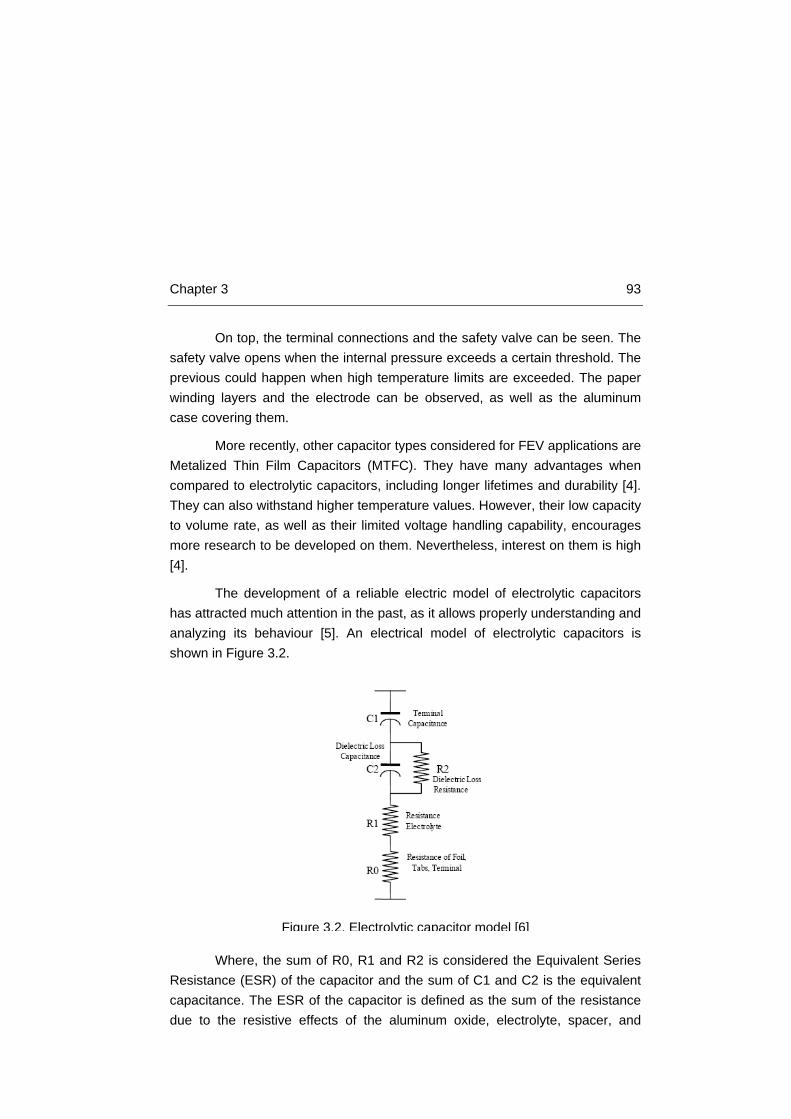
Chapter 3 93

On top, the terminal connections and the safety valve can be seen. The safety valve opens when the internal pressure exceeds a certain threshold. The previous could happen when high temperature limits are exceeded. The paper winding layers and the electrode can be observed, as well as the aluminum case covering them.

More recently, other capacitor types considered for FEV applications are Metalized Thin Film Capacitors (MTFC). They have many advantages when compared to electrolytic capacitors, including longer lifetimes and durability [4]. They can also withstand higher temperature values. However, their low capacity to volume rate, as well as their limited voltage handling capability, encourages more research to be developed on them. Nevertheless, interest on them is high [4].

The development of a reliable electric model of electrolytic capacitors has attracted much attention in the past, as it allows properly understanding and analyzing its behaviour [5]. An electrical model of electrolytic capacitors is shown in Figure 3.2.

Where, the sum of R0, R1 and R2 is considered the Equivalent Series Resistance (ESR) of the capacitor and the sum of C1 and C2 is the equivalent capacitance. The ESR of the capacitor is defined as the sum of the resistance due to the resistive effects of the aluminum oxide, electrolyte, spacer, and

Figure 3.2. Electrolytic capacitor model [6]

94 Failure Modes & Failure Precursor Parameters

electrodes (foil, tabbing, leads, and ohmic contacts). This parameter is of paramount importance for capacitor RUL estimation. Other researches also include the inductive effect due to the wound structure of the capacitor, which is represented by the L or Equivalent Series Inductance (ESL). It can be observed in Figure 3.3 [2].

Consequently, the impedance of the capacitor is frequency dependent; this is an important fact for measuring the ESR parameter. The resonant frequency is calculated as:

𝑓𝑟 = 12𝜋√𝐸𝑆𝐿∗𝐶

(Eq. 3.1)

The previous behavior can be demonstrated through Figure 3.4, where the complex impedance Z is plotted versus the frequency. The figure belongs to the bode plot of a capacitor of 4700 μF. It can be observed that there are three separated frequency bands. The capacitance is dominant in the low-frequency band (Hz), the ESL in the high-frequency band (MHz) and the ESR in the mid-frequency one (kHz).

Figure 3.4. Capacitor impedance vs frequency plot

Figure 3.3. Electrolytic capacitor model [2]

Chapter 3 95

3.2 Electrolytic capacitor failure modes Now that the main physical characteristics of electrolytic capacitors have

been introduced, the failure modes and mechanisms will be reviewed. Most common faults in electrolytic capacitors include catastrophic failures due to manufacturing process introduced defects or wrong component selection, and gradual faults, which cannot be avoided [1]. Capacitors degradation process is well known under certain operating conditions (environmental temperature, voltage level, current, etc.). Manufacturers provide a reference lifetime of operating hours depending on the environmental conditions and the capacitor package type [3]. However, it only considers stationary conditions, and not varying operating conditions. Thus, preventive maintenance has been mostly employed on these components, simply replacing them after a given number of operating hours, independently of their real healthy state.

The failure modes of electrolytic capacitors and root causes have been widely studied [6, 7, 8]. Degradation of these components is due to a combined effect of electrical, thermal, mechanical, and environmental stresses [7]. Its main degradation mechanism is caused by the vaporization of the electrolyte, which is strongly influenced by the capacitor working temperature [9]. The following operating parameters, voltage, current and frequency are known to have second order effects regarding the operating temperature of the capacitor, and thus, on the degradation process of it; however, their correlation with the temperature and the degradation has not been strictly determined. It is assumed that they affect at different degrees the internal temperature of the capacitor, which is the one directly degrading it.

High electrical stress is known to accentuate the degradation of the oxide layer due to localized dielectric breakdown [7], although high electrical stresses are related to sudden failure causes. The literature on capacitor degradation shows a direct relationship between electrolyte decrease and increase in the ESR of capacitor [10]. An ESR increase implies a slow decrease in the average output voltage as well.

Another mechanism occurring simultaneously is the increase of the internal pressure due to an increased rate of chemical reactions, which are attributed to the internal temperature increase in the capacitor due to the

96 Failure Modes & Failure Precursor Parameters

activation of chemical reactions. A FMEA analysis was developed for electrolytic capacitors in [1]. It is shown in Figure 3.5.

This FMEA shows the different failures modes. In this summary, either gradual or sudden failures that could take place are shown. In this thesis, the main focus is failures due to the degradation with time, this is, gradual failures and not sudden failures, following the conclusions that were observed in Chapter 2.6 for sudden failures and why their study was discarded.

The different literature studies state that the degradation of capacitors involves a loss of functionality. The main consequences of gradual degradation are a decrease in capacitance and an increase in the ESR, which further increases the losses, and therefore, the internal temperature, accelerating the degradation process [8].

Figure 3.5. FMEA electrolytic capacitors [1]

Chapter 3 97

Manufacturers suggest the following guidelines to define the end of life of a component [1, 3]:

• ESR > 2 x initial ESR value.

• Variation of the initial capacitance > 10 %.

• Leakage current > specified on datasheet.

As a consequence, the previous guidelines are commonly considered as failure thresholds to replace the capacitor.

3.2.1 Electrolytic capacitors failure mode conclusions The most reported gradual failure mode of electrolytic capacitors is

electrolyte vaporization, mainly produced by thermal stresses. The thermal stresses might be influenced by other factors such as the voltage level and the frequency range of operation. However, models describing the relationship of voltage and frequency to the operating temperature have not been discovered on the literature.

It is observed that most researches claim that a direct consequence of the thermal stresses is an increase of the internal pressure and of the leakage current, as well as a variation of the capacitance and the ESR.

3.3 Electrolytic capacitor failure precursor parameters

Following the analysis done on electrolytic capacitor failure modes, it has been observed that the different authors suggest the following variables as possible failure precursor parameters related to the time degradation of capacitors [4, 6, 7, 8, 11, 12, 13]:

• Capacitance

• ESR

• Temperature

• Leakage current

98 Failure Modes & Failure Precursor Parameters

• Internal pressure

Other prognostic approaches for switched mode power supplies were presented in [6, 14, 15]. One of the approaches consisted on measuring the power losses of the capacitor, which could be attributed to the ESR, and thus, an indirect measurement of it [6]. On the other approaches, the output ripple voltage and leakage current were presented as a function of time and degradation level of the capacitor, but there was not an associated physics model of the degradation. Finally, manufacturers claim that internal pressure and temperature are failure precursor parameters [1].

3.3.1 Conclusions on failure precursor parameters for electrolytic capacitors monitoring

Having analyzed the different possibilities suggested on the literature review, the selected failure precursor parameters to be further studied and monitored in the accelerated aging tests were: the capacitance, the ESR and the surface temperature. The reasons to select them will be now explained.

On the first hand, the output ripple voltage and the leakage current were discarded for several reasons. They can be affected by the operating conditions of the rest of the components in the circuit. In case other component fails or misbehaves, it could be reflected in those parameters. Another negative aspect is that they would require accurate measurements under varying operating conditions, which would require high sampling rates and processing memory. These features are not compatible with a PHM system for online monitoring the health state of FEV components.

Internal temperature and pressure would have been good candidates for PHMS, unless for their intrusiveness. Opening the case and introducing a sensor is not a sensible change for a system operator. A possible suggestion for capacitor manufacturers would be to provide the components with integrated sensors; however, this is not the case yet.

Finally, the selection of the failure precursor parameters is explained. A major positive point is that the capacitance and the ESR have shown good prognosticability on the reviewed researches [7]. Given the high impact of the temperature on the degradation process and the variation of the ESR with

Chapter 3 99

respect to the measurement temperature, the surface temperature was also selected to be monitored. A major advantage of these variables is that they have good trendability during component lifetime, thus, they do not need to be continuously monitored with high sampling rates. They are also measurable from the connection terminals, therefore, they are not considered intrusive.

Cost is a key point that must be taken into account for online monitoring of the suggested variables. In lab environments measurements are carried out with expensive RLC meters. Thus, the measurement of ESR and capacity for vehicle on-board systems will require self-developed equipment, which is explained in Chapter 4.

3.4 Insulated Gate Bipolar Transistors (IGBT) physics

IGBT is a semiconductor device that combines the high current and voltage capabilities of a Bipolar Junction Transistor (BJT) and the gate drive characteristics of a Metal-Oxide Semiconductor Field-Effect Transistor (MOSFET). Hence, the IGBT is a minority carrier device with high input impedance and high current carrying capability. The structure of an IGBT is similar to that of a vertical diffusion power MOSFET, except for an additional p+ layer above the collector [16]. The additional p+ layer in the IGBT acts as a source of holes that are injected into the drift region during operation. These injected holes enable quick turn-off by recombination with the excess of electrons that remain in the body of the IGBT after switch-off. Figure 3.6.a represents the schematic structure of the IGBT [24].

100 Failure Modes & Failure Precursor Parameters

(a)

(b)

Figure 3.6. (a) IGBT schematic [4]; (b) IGBT schematic with parasitic

elements [17]

Chapter 3 101

Figure 3.6.b shows the schematic of the IGBT with the parasitic elements. These are:

• Three pn-junctions J1, J2, J3.

• One pnp-transistor structure T1.

• One npn-transistor structure T2.

• One diode structure D1.

• One thyristor structure V1.

• One MOSFET structure T3.

• One JFET structure T4 between two adjacent IGBT cells.

Parasitic elements play a key role in failure mechanisms of IGBTs, being the root cause of several failure modes.

Compared to MOSFETs, IGBTs are better suited to scale in current handling capability at higher voltage levels due to their bipolar output characteristics. On the other hand, IGBT turn on and turn off times are bigger, increasing overall switching losses, and thus, reducing efficiency. The IGBT has a high current fall time that restricts the use of IGBT to moderate frequencies operation (less than 50 kHz) in conventional PWM switching applications. Since most automotive motor drive applications work in this frequency range, the IGBT is usually selected [18, 19].

Regarding IGBT employment, one of the main problems arose when placing them in parallel for higher power rates [17]. First generation IGBTs, the so-called punch-through (PT) IGBTs, had a negative thermal coefficient (NTC). This means that if one of the paralleled components gets hotter, it becomes more conductive, and thus, it carries higher current values. This would end up with a thermal runaway of the IGBT. However, the successive IGBT technologies (non punch-through, Trench-FS) overcome this problem, obtaining positive thermal coefficients (PTC). Figure 3.7 shows a comparison of the different IGBT technologies [16, 17]. Some other names have been given to similar technologies; however, this is done depending on the manufacturer. It must be noticed the different die sizes required for each one, which has contributed to the reduction of manufacturing costs.

102 Failure Modes & Failure Precursor Parameters

A final consideration when talking about IGBTs is their package technology. In fact, the most important degradation mechanisms are associated to it, rather than to the electric behavior of the component. The manufacturing process and package technology influence on IGBT reliability were reported in both the LESIT project [20] and the research developed by Bayerer et al. [21]. The package of an IGBT module is shown in Figure 3.8.

Figure 3.7. IGBT technologies overview [9]

Chapter 3 103

The main functionality of the IGBT is contained in the IGBT die, where the different Silicon substrates (see Figure 3.6) are manufactured. The rest of the package is mainly a support for the functioning of the die. Bonding wires are commonly made of aluminum, they provide the means for electrical connection between the die and the terminals; depending on the manufacturer process it may connect either to the emitter or the collector. The die is connected to a substrate and then to a base plate, through solder joints of the sequential layers. The aim is to dissipate the heat generated on the die, through the base plate, usually made of copper. The encapsulant is made of epoxy or resin, which is intended to provide higher electrical insulation than air to avoid the formation of electrical arcs. The temperature reached in the junction between the die and the die solder is called the junction temperature. This temperature is critical for IGBT reliability [20-24], as the highest temperature values are reached there. A critical parameter of IGBT design is junction-to-case thermal resistance (Rthj-c). The lower the Rthj-c is, the better for the reliability of the component. It provides information regarding heat transfer from the junction to the base plate, where the heat is dissipated. It must be noticed that IGBT manufacturing package includes layers of different materials, such as copper (base plate), aluminum (bonding wires), silicon (die) and SnPb40Ag1 (solder joint).

Figure 3.8. IGBT module package overview [22]

104 Failure Modes & Failure Precursor Parameters

3.5 IGBT failure modes Factors affecting IGBT reliability during its operational life are various:

electrical loading, mechanical vibration and environmental conditions, etc. Most of them have influence on the junction temperature variation, which is claimed to be the most important degradation force for IGBTs [20-24]. For example, the electrical traction drive for an urban tram may experience 106-108 power cycles, with temperature swings up to 80 ºC during its lifetime [23]. The effects of temperature swings critically affect IGBT reliability and lifetime. Figure 3.9 shows the improvement on IGBT reliability in recent years, reducing the failure rate from 1000 FIT (failures-in-time, tipically, 10−9 failures/h) in 1995 to 20 FIT in 2000 [21]. This change is the result of improvements introduced on the manufacturing processes and package design. Much improvement has been made regarding solder-joint bonding and junction-to-case thermal resistance reduction. Hence, on the one hand, the electrical path is secured through a better bonding, and besides, heat is more efficiently removed to the cooling plate.

Figure 3.9. Device (IGBT) FIT rate evolution [22]

Chapter 3 105

Several previous projects studied IGBT reliability. Among them, the LESIT project investigated the reliability of IGBT modules for traction applications, including IGBT bond-wire liftoff and solder fatigue [23]. The physics-based model extracted from it was refined in [21]. The EU RAPSDRA project improved and achieved agreement on standardized accelerated tests. The outcome from most of these projects is the research on IGBT failure mechanisms analysis and the presentation of methods to improve the reliability, such as precursor parameter identification for condition monitoring. In [24] a FMEA shown in Table 3.1 was presented as an example. It shows some potential failures sites on IGBTs, together with the potential failure modes, the causes and the mechanisms. A deeper insight of all of them is reviewed in sections 3.5.1 and 3.5.2.

In [25], a FMEA analysis was also developed showing the failures as a consequence of poor handling or selection of the component (extrinsic mechanisms).

Potential Failure

Sites

Potential Failure

Modes

Potential Failure

Causes

Potential Failure

Mechanisms

Oxide

Short circuit, loss of

gate control, increased

leakage current

High temperature,

high electric field,

overvoltage

Time Dependent

Dielectric Breakdown

(TDDB)

Oxide,

oxide/substrate

interface

High leakage current Overvoltage, high

current densities Hot-electrons

Device body Loss of gate control,

device burn-out

High electric field,

overvoltage, ionizing

radiation

Latch-up

Table 3.1. FMEA for IGBT failures [24]

106 Failure Modes & Failure Precursor Parameters

The previous two figures show failures of IGBTs commonly observed in real applications, when a wrong selection of components is done. There is an extended feeling that semiconductors failure rate is high due to the previous figures, which include extrinsic (sudden) failure mechanisms. Although the literature is wide regarding sudden failures on semiconductors devices, in this research it is assumed that these failure types have been overcome through testing prior to the component operation, and we will be focusing on gradual failures. Regarding gradual failures, only time dependent dielectric breakdown was considered in [24].

Figure 3.10. IGBT FMEA for extrinsic mechanisms [25]

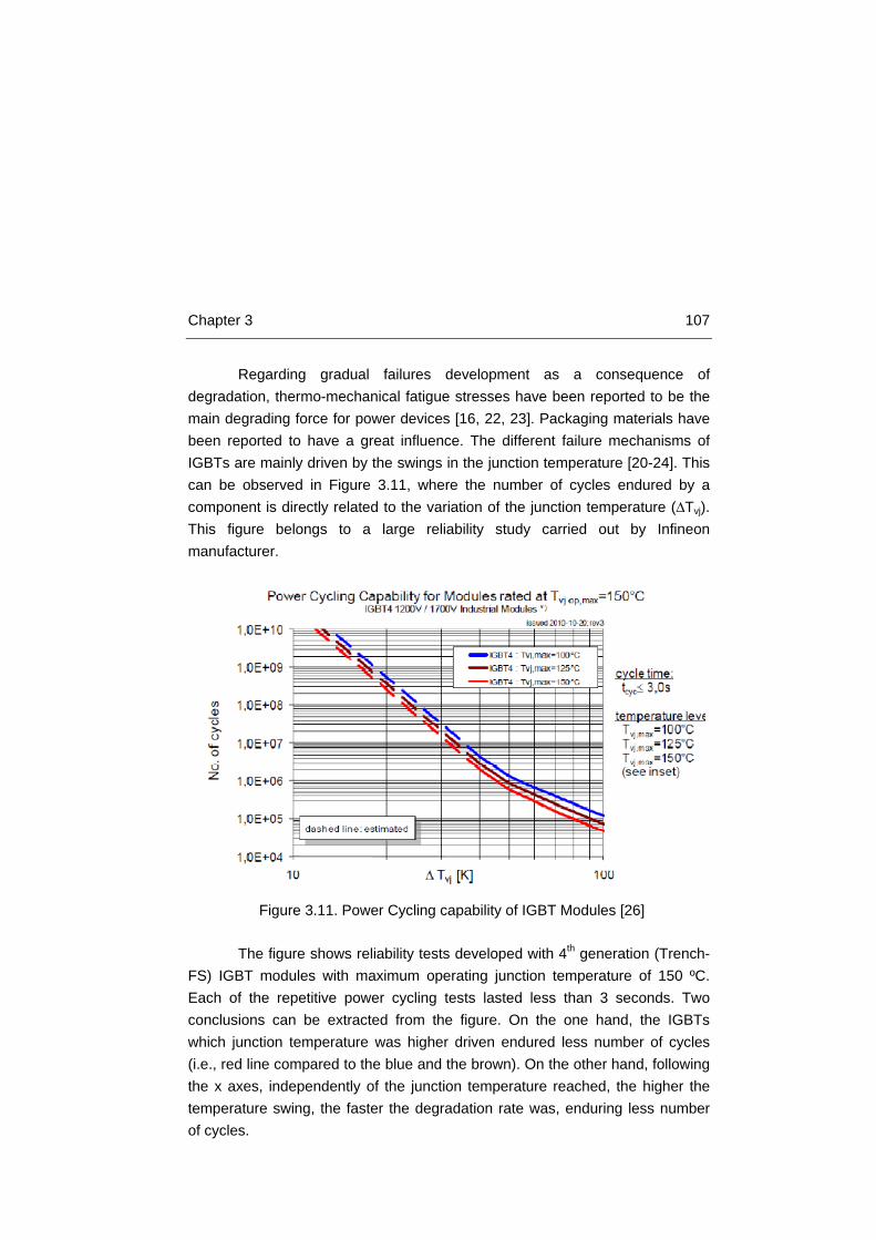
Chapter 3 107

Regarding gradual failures development as a consequence of degradation, thermo-mechanical fatigue stresses have been reported to be the main degrading force for power devices [16, 22, 23]. Packaging materials have been reported to have a great influence. The different failure mechanisms of IGBTs are mainly driven by the swings in the junction temperature [20-24]. This can be observed in Figure 3.11, where the number of cycles endured by a component is directly related to the variation of the junction temperature (∆Tvj). This figure belongs to a large reliability study carried out by Infineon manufacturer.

The figure shows reliability tests developed with 4th generation (Trench-FS) IGBT modules with maximum operating junction temperature of 150 ºC. Each of the repetitive power cycling tests lasted less than 3 seconds. Two conclusions can be extracted from the figure. On the one hand, the IGBTs which junction temperature was higher driven endured less number of cycles (i.e., red line compared to the blue and the brown). On the other hand, following the x axes, independently of the junction temperature reached, the higher the temperature swing, the faster the degradation rate was, enduring less number of cycles.

Figure 3.11. Power Cycling capability of IGBT Modules [26]

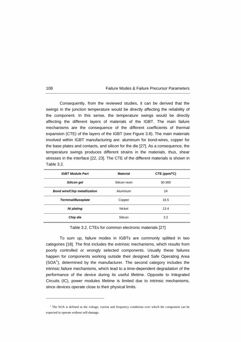
108 Failure Modes & Failure Precursor Parameters

Consequently, from the reviewed studies, it can be derived that the swings in the junction temperature would be directly affecting the reliability of the component. In this sense, the temperature swings would be directly affecting the different layers of materials of the IGBT. The main failure mechanisms are the consequence of the different coefficients of thermal expansion (CTE) of the layers of the IGBT (see Figure 3.8). The main materials involved within IGBT manufacturing are: aluminum for bond-wires, copper for the base plates and contacts, and silicon for the die [27]. As a consequence, the temperature swings produces different strains in the materials, thus, shear stresses in the interface [22, 23]. The CTE of the different materials is shown in Table 3.2.

IGBT Module Part Material CTE (ppm/ºC)

Silicon gel Silicon resin 30-300

Bond wire/Chip metallization Aluminum 24

Terminal/Baseplate Copper 16.5

Ni plating Nickel 13.4

Chip die Silicon 3.2

Table 3.2. CTEs for common electronic materials [27]

To sum up, failure modes in IGBTs are commonly splitted in two categories [18]. The first includes the extrinsic mechanisms, which results from poorly controlled or wrongly selected components. Usually these failures happen for components working outside their designed Safe Operating Area (SOA1), determined by the manufacturer. The second category includes the intrinsic failure mechanisms, which lead to a time-dependent degradation of the performance of the device during its useful lifetime. Opposite to Integrated Circuits (IC), power modules lifetime is limited due to intrinsic mechanisms, since devices operate close to their physical limits.

1 The SOA is defined as the voltage, current and frequency conditions over which the component can be

expected to operate without self-damage.

Chapter 3 109

IGBT failure mechanisms have also been divided from a different point of view, which is depending on the place of the failure. They are: chip-related failures and package related failures. Provided their importance in the following studies each of them is briefly addressed.

3.5.1 Chip-related failures Chip related failures are the ones that ultimately destroy the device,

disabling any possibility of normal operation. Although they are splitted from package-related failures, both may be interlinked for a failure event. Most reported chip-related failures are:

1. Transient Electrical Stresess: Electrostatic discharge (ESD) and Electrical Overstress (EOS) would be included within this group. Both of them provide similar failure modes [22, 23, 27], including gate oxide puncture and internal short circuit. ESD failure is related to inappropriate handling of the device. Meanwhile, EOS is associated to voltage and current conditions outside of the component SOA. Heating effects due to overvoltage conditions and heat sinking may lead to component destruction. Large 𝜕𝑖

𝜕𝑡 values could also contribute

to component heating.

2. Latch-up and Triggering of parasitics: Switch on and especially, switch off times must be properly calculated. Loss of gate control or latch-up failures may appear due to large 𝜕𝑣

𝜕𝑡 during the switch off

process of the component, triggering the inherent parasitic thyristor of IGBT body [25]. High junction temperature also contributes to this failure.

3. Time Dependent Dielectric Breakdown (TDDB): Dielectric breakdown occurs when a strong electric field induces a current channel through an originally insulated medium. High temperature and strong electric field may impart energy into an electron or a hole which becomes a “Hot Carrier”. It gets enough energy to overcome the energy barrier and to be injected into the gate oxide by tunneling, resulting in charge trap and interface state generation [28]. The latter may lead to shifts in the performance characteristics of the device, i.e. the threshold

110 Failure Modes & Failure Precursor Parameters

voltage, transconductance; ultimately leading to the loss of gate control.

4. Electromigration: This is a wear-out mechanism in silicon interconnection owing to high current densities. Extremely high density current flows displace atoms within thin-film conductors, leaving a void at one end. The formation of the void causes open circuit or high resistive paths.

5. External radiation - Cosmic rays: There is a minute probability of high energy mobile ions and neutrons travelling on space to hit the devices. This produces tunneling and destruction of the chip. This failure mode is rare [25]. In [29], a figure of the damage caused by a cosmic ray is shown (see Figure 3.12).

Figure 3.12. Cosmic ray caused damage [29]

Chapter 3 111

3.5.2 Package-related failures Package-related failures are, as the name says, failures due to the way

components are manufactured and layers of materials assembled (see Figure 3.8). Package-related failures are reported to be the main cause of time-dependent degradation processes. The most frequently reported package related failure modes are: bond wire lift off and solder fatigue [22, 23]. Bond wire lift off is a consequence of crack growth at the bond wire/chip interface. Solder fatigue is the propagation of cracks or voids between the module substrate and base plate. They are explained below.

1. Bond-wire lift off: Bond wire lift off is a consequence of crack growth at the bond wire/chip interface. Owing to temperature swings and different CTEs between Silicon and Aluminum. The difference in strain in both materials creates a stress in the interface. These strain-stress cycles initiate cracks that propagate, ending with the wire complete disconnection [23]. The process is shown in Figure 3.13.

A bond-wire liftoff failure can be observed in a real component on Figure 3.14, when observed through Scanning Electron Microscope (SEM).

Figure 3.13. Bond-wire lift off process [6]

112 Failure Modes & Failure Precursor Parameters

Bond-wire heel cracking rarely occurs on advanced IGBTs, although it can be observed after long endurance tests [5]. An example can be observed in Figure 3.15.

2. Solder fatigue: Solder fatigue is the propagation of cracks or voids between the module substrate and the base plate and/or the device chip and substrate. Solder fatigue arises because of the different CTEs of the silicon die and copper substrate, resulting in shear stresses in the solder layer. In the case of solder, elastic, plastic and creep-induced strains are all significant. Eventually, leading to cracks and voids formation. Due to the creep strain, and the relationship of the crack length with the number of thermal cycles, Arrhenius Law has been employed to explain this degradation process [21]. The propagation of voids reduces the effective area to dissipate heat, and

Figure 3.15. Bond-wire heel cracking IGBT [5]

(a) (b)

Figure 3.14. Bond-wire lift off examples [34]

Chapter 3 113

thus, the thermal resistance (RTH) is increased. Ultimately, thermal runaway is the critical failure. In Figure 3.16 and Figure 3.17 the process of solder fatigue is shown. More precisely Figure 3.16 shows the most common solder fatigue failures depending on the junction temperature swings. The tests developed in [6] show that temperature swings bigger than 100 K destroyed faster the bond wire solder; meanwhile, swings smaller that 80 K destroyed faster chip/base-plate interface. Figure 3.17 shows the latter case.

Figure 3.17. Solder fatigue crack propagation [6]

Figure 3.16. Solder fatigue [6]

114 Failure Modes & Failure Precursor Parameters

3.5.3 IGBT failure mode conclusions A large amount of researches have dealt with the problem of assessing

the failure modes and mechanisms in IGBTs. The reported gradual failure modes with higher importance are package related failures: a) bond-wire liftoff and b) solder fatigue. Chip-related failures have also been investigated, but their identification is done through the analysis of the atomic structure of the component. In this sense, advanced microscopy techniques (Scanning Electron Microscope (SEM) and Scanning Acoustic Microscope (SAM) have been employed to assess them. Whereas, package related failures are analyzed through optic microscopes.

Finally, in this research we will be focusing on the identification of the failures taking place at package level which are the failures directly related to gradual degradation due to temperature variations.

3.6 IGBT Failure Precursor Parameters IGBT health state estimation is an incredibly challenging task. The

stochasticity of the degradation process has been demonstrated [24], showing different degradation patterns even for the same IGBT types. Furthermore, the continuously varying operating conditions of traction applications forces to carefully select the appropriate physical characteristics to be monitored.

IGBT failure precursor parameters have been widely studied [20-24]. A great number of researches focus on junction temperature measurement. Junction temperature measurement allows junction-to-case thermal resistance measuring (RTHj-c) and the application of thermal models. The latter researches employ the measurement of the junction temperature to supply with information Finite Element Analysis (FEM) or mathematical approaches. Then, the employment of a cycles counting algorithm [32] is employed for average and swing temperatures assessment. Finally, this kind of techniques relies on physics-based thermal models (i.e. Arrhenius law) which employ the counted average and swing temperatures to assess the degradation state. As it can be observed, the complexity of the procedure is high with poor results [22, 23].

Chapter 3 115

It needs to be considered that an IGBT is a three terminal component. Therefore, apart from temperature monitoring, the measurement of currents and voltages at the terminals have been suggested in different ways.

The possibility of assessing the degradation state of the IGBT through ringing characterization was studied in [33]. The ringing of the voltage on inductive switching of the IGBT was analyzed with successful results. However, the measuring accuracy and sampling rates (MHz) were very high. In [24], a gate capacitance variation was observed for degraded components. A variation of the switching on times and of the gate threshold voltage (VGE,TH) were also observed.

In Hensler et al. [25], Smet et al. [34], and Patil et al. [24] accelerated aging tests were performed on IGBT modules. The authors observed changes in the values of collector-emitter on-state voltage (VCE,ON) and thermal resistance (RTHj-c) before IGBT failure. Thermal resistance was measured through thermo-optical sensors. The required accuracy was very high and it implied measuring the junction and the baseplate temperatures under a fixed thermal flux. A criterion adopted for IGBT failure was a variation higher than 20 % for RTHj-c. Therefore, the measurements were made at regular intervals. It was observed that crack and voids propagation due to the degradation increased the RTHj-c. Regarding the variation of the VCE,ON, changes of 2 to 4 % were observed. Measurement accuracy on the decades of volts was required. On-state resistance (RON), has also been included in some studies [23], however, this is a term more employed for MOSFETs. RON stands for the fraction of the VCE,ON by the instantaneous flowing current.

Consequently, different variables have been suggested and employed for failure precursor parameters. Gate signal analysis, switching times, junction-to-case thermal resistance and collector-emitter on state voltage have been proposed. They are now summarized with their corresponding definition [23]:

• VCE,ON: collector-emitter voltage when the IGBT is on-state.

• VGE,TH: gate-emitter threshold voltage. It stands for the measured gate voltage at which the IGBT is considered to be in the on-state.

• Switching times (TON, TOFF): transition times from the on-state to off-state and vice versa.

116 Failure Modes & Failure Precursor Parameters

• TJ: junction-temperature. Temperature measured at the closest point to the die.

• RTHj-c: junction-to-case thermal resistance. Heat transfer capability from junction to case measured as: 𝑅𝑇𝐻𝑗−𝑐 = 𝑇𝐽−𝑇𝐶

𝑉𝐶𝐸,𝑂𝑁∗𝐼𝑂𝑁, where TC is

the case temperature, and ION is the on-state current.

These physical characteristics were summarized in [22]. Figure 3.18 compiles them and some of their pros and cons.

3.6.1 Conclusions on failure precursor parameters for IGBT monitoring

Once the different possibilities suggested on the literature review were analyzed, the failure precursor parameters were selected. The physical characteristics selected to be monitored during the accelerated aging tests were:

• Collector-emitter voltage (VCE).

• Collector current (IC).

• Case temperature (TC).

• Gate voltage (VG).

• Gate current (IG).

Figure 3.18. Pros and cons failure precursor parameters [23]

Chapter 3 117

These variables allow monitoring the following failure precursor parameters, VCE,ON and VGE,TH. The gate current (IG) parameter was initially selected in order to monitor the gate in the switching events. If the gate capacitance changes with the degradation, the current consumption during these transient periods could change as well.

Different issues with respect to the discarded failure precursor parameters are discussed now. Firstly, the junction temperature (TJ) was discarded for one reason, its intrusiveness [7, 24]. Some manufacturers have started to implement on-chip temperature sensors on their IGBT modules, but still, they claim to have some difference with respect to the junction temperature [17], as well as possibly electrical noise adding to the measurements in tractive applications. Therefore, accurately monitoring the TJ is an unsolved problem. Furthermore, it would be impossible to have access to the inner side of the component in discrete IGBTs, which are encapsulated in polymer. As a consequence of avoiding TJ monitoring, RTH monitoring was restricted as well. Finally, although the selected parameters allowed monitoring the switching times (TON and TOFF) of the IGBT, they were discarded. High sampling rates (MHz) and measuring accuracies are required, as well as complex data processing at high speeds.

3.7 General conclusions of Failure Mode and Failure Precursor Parameters

First, the physics of both components have been explained. Their structure and package have been deeply analyzed. This knowledge allowed understanding the most common failure modes and mechanisms reported by different researches. On this basis, failure precursor parameters related to them were studied.

Finally, a preliminary selection of the failure precursor parameters to be monitored in this research has been done, following the criteria and features defined in Chapter 1 for PHM development. The next Chapter will study the behavior of the selected failure precursor parameters during the degradation process through the development of accelerated aging tests. The problems arising from the measurement of failure precursor parameters will be also treated.

118 Failure Modes & Failure Precursor Parameters

3.8 References [1] “Technical Guide of Aluminum Electrolytic Capacitor,” Panasonic, Matsushita

Electronic Components Co Ltd, Capacitor Division, March 2000

[2] A. M. Imam; “Condition monitoring of electrolytic capacitors for power electronics applications,” PhD Thesis, Georgia Institute of Technology, 2007

[3] ALS30 series datasheet. Available online on: http://www.kemet.com/Lists/ProductCatalog/Attachments/389/KEM_A4031_ALS30_31.pdf

[4] J. Flicker, R. Kaplar, M. Marinella and J. Granata, "Lifetime testing of metallized thin film capacitors for inverter applications," Photovoltaic Specialists Conference (PVSC), 2013 IEEE 39th, Tampa, FL, pp. 3340-3342, 2013

[5] M. Hao, and L. Wang, “Fault diagnosis and failure prediction of aluminum electrolytic capacitors in power electronic converters, Industrial Electronics Society,” IECON 2005, 31st Annual Conference of IEEE, pp. 6., 2005

[6] E.C. Aeloíza, J. Kim, P. Enjeti and P. Ruminot, "A real time method to estimate electrolytic capacitor condition in PWM adjustable speed drives and uninterruptible power supplies," Power Electronics Specialists Conference, 2005. PESC'05. IEEE 36thIEEE, pp. 2867, 2005

[7] J. Celaya, C. Kulkarni, S. Saha, G. Biswas, and K. Goebel, "Accelerated aging in electrolytic capacitors for prognostics," Reliability and Maintainability Symposium (RAMS), 2012 Proceedings - Annual, pp. 1. 2012

[8] C. Kulkarni, J. Celaya, K. Goebel, and G. Biswas, "Bayesian framework approach for prognostic studies in electrolytic capacitor under thermal overstress conditions," Proceedings of the Annual Conference of the Prognostics and Health Management Society, pp. 503, 2012

[9] C. Kulkarni, G. Biswas, X. Koutsoukos, J. Celaya, K. Goebel, ”Integrated diagnostic/prognostic experimental setup for capacitor degradation and health monitoring,” IEEE AUTOTESTCON, 2010

[10] J. Celaya, C. Kulkarni, G. Biswas, S. Saha and K. Goebel, “A Model-based Prognostics Methodology for Electrolytic Capacitors Based on Electrical

Chapter 3 119

Overstress Accelerated Aging,” Annual Conference of the Prognostics and Health Management Society, 2011

[11] K. Abdennadher, P. Venet, G. Rojat, J.M. Rétif, C. Rosset, “A real-time predictive-maintenance system of aluminum electrolytic capacitors used in uninterrupted power supplies,” in Industry Applications, IEEE Transactions on, vol. 46, pp. 1644-1652, 2010

[12] A. Braham, A. Lahyani, P. Venet, N. Rejeb, ”Recent developments in fault detection and power loss estimation of electrolytic capacitors,” in Power Electronics , IEEE Transactions on, 25 (1), art. no. 5200514, pp. 33-43, 2010

[13] M.A. Vogelsberger, T. Wiesinger, H. Ertl, “Life-cycle monitoring and voltage-managing unit for DC-link electrolytic capacitors in PWM converters,” in Power Electronics, IEEE Transactions on, vol. 26, no. 2, pp. 493-503, 2011

[14] D. Goodman, J. Hofmeister, and J. Judkins, “Electronic prognostics for switched mode power supplies,” Microelectronics Reliability, vol. 47, pp. 1902-1906, 2007

[15] J.B. Judkins, J. Hofmeister, and S. Vohnout, “A prognostic sensor for voltage regulated switch-mode power supplies,” in Aerospace conference, 2007 IEEE, pp. 1-8, 2007

[16] N. Patil, “Prognostics of Insulated Gate Bipolar Transistors,” PhD Thesis, University of Maryland, 2011

[17] A. Volke and M. Hornkamp, “IGBT Modules. Technologies, Driver and Application,” Infineon Technologies AG, Munich, 2nd Edition, 2015

[18] M. Ciappa and Alberto Castellazi; “Reliability of High-Power IGBT Modules for Traction applications”, in 45th Annual International Reliability Physics Symposium, Phoenix, 2007

[19] M. Denk and M. Bakran;, “Online Junction Temperature Cycle Recording of an IGBT Power Module in a Hybrid Car,” Advances in Power Electronics, 2015

[20] R. Amro, J. Lutz, J. Rudzki, R. Sittig and M. Thoben, "Power Cycling at High Temperature Swings of Modules with Low Temperature Joining Technique,"

120 Failure Modes & Failure Precursor Parameters

Power Semiconductor Devices and IC's, 2006. ISPSD 2006. IEEE International Symposium on, pp. 1, 2006

[21] R. Bayerer, T. Herrmann, T. Licht, J. Lutz, and M. Feller, "Model for Power Cycling lifetime of IGBT Modules: various factors influencing lifetime," Integrated Power Systems (CIPS), 2008 5th International Conference on VDE, pp. 1, 2008

[22] H. Oh, B. Han, P. McCluskey, C. Han and B.D. Youn, "Physics-of-Failure, Condition Monitoring and Prognostics of Insulated Gate Bipolar Transistor Modules: A Review," in Power Electronics, IEEE Transactions on, vol. 30, pp. 2413-2426, 2015

[23] Yang, S., Xiang, D., Bryant, A., Mawby, P., Ran, L. and Tavner, P., "Condition monitoring for device reliability in power electronic converters: a review," in Power Electronics, IEEE Transactions on, vol. 25, no. 11, pp. 2734-2752, 2010

[24] N. Patil, J. Celaya, D. Das, K. Goebel and M. Pecht, "Precursor Parameter Identification for Insulated Gate Bipolar Transistor (IGBT) Prognostics," in Reliability, IEEE Transactions on , vol.58, no.2, pp.271-276, June 2009

[25] A. Hensler, J. Lutz, M. Thoben, K. Guth;, "First power cycling results of improved packaging technologies for hybrid electrical vehicle applications," in 6th International Conference on Integrated Power Electronics Systems (CIPS), Mar 16-18. IEEE, 2010

[26] Infineon’s AN2010-02, Technical Information IGBT modules, Use of Power Cycling curves for IGBT 4.

[27] B. Ji, “In-situ Health Monitoring of IGBT,” PhD Thesis, University of Newcastle, 2011

[28] J.B. Bernstein, M. Gurfinkel, X. Li, J. Walters, Y. Shapira and M. Talmor,;”Electronic circuit reliability modeling,” Microelectronics Reliability, vol. 46, no. 12, pp. 1957-1979, 2006

[29] D.J. Chamund, L. Coulbeck, D.R. Newcombe, P.R. Waind, ”High power density IGBT module for high reliability applications,” in Power Electronics and Motion Control Conference, 2009. IPEMC'09. IEEE 6th International, pp. 274-280, IEEE. 2009

Chapter 3 121

[30] M. Ciappa; “Selected failure mechanisms of modern power modules,” in Microelectronics Reliability, vol. 42, pp. 653-667, 2002

[31] A. Morozumi, K. Yamada, T. Miyasaka, S. Sumi and Y. Seki “Reliability of Power Cycling for IGBT Power Semiconductor Modules,” in Industrial Applications, IEEE Transactions on, vol. 39, no. 3, 2003

[32] M. Matsuishi and T. Endo, “Fatigue of metals subjected to varying stress,” Japan Society of Mechanical Engineers, Fukuoka, Japan, 37-40, Mar. 1968

[33] A. Ginart, M.J. Roemer, P.W. Kalgren, K. Goebel, “Modeling Aging Effects of IGBTs in Power Drives by Ringing Characterization,” 2008 International Conference on Prognostics and Health Management, 2008

[34] V. Smet, F. Forest, J. Huselstein, F. Richardeau, Z. Khatir, S. Lefebvre, M. Berkani, "Ageing and Failure Modes of IGBT Modules in High-Temperature Power Cycling," in Industrial Electronics, IEEE Transactions on, vol. 58, no. 10, pp. 4931-4941, 2011

Chapter 4

4 Accelerated Aging Tests

In the previous chapter, the failure modes and candidate failure precursor parameters of the two most critical components of the inverter were analyzed with a deep literature review. However, in the way for the implementation of the PHM system, failure modes and failure precursor parameters need to be confirmed. In this basis, data belonging to the degradation process of both components is required, as we stated in Chapter 1 and 2. Therefore, the development of accelerated aging tests is explained now.

A major issue about experiments development is the hardware architecture to measure the different physical characteristics. Measurement types and accuracy are critical aspects that need to be clarified before experiments development. Hence, this Chapter follows the next guideline for each of the components (capacitor and IGBT):

1. Failure precursor monitoring hardware. The hardware employed for laboratory tests and the hardware that would be employed in online tests is explained.

2. Accelerated Aging Tests Mode. A description of the development of the accelerated aging tests is provided.

3. Accelerated Aging Tests Results.

124 Accelerated Aging Tests

Failure precursor monitoring hardware section is especially important for its relevance on the PHM system configuration. It is on the way hardware is implemented that the features considered for the PHMS on Chapter 1 should be compiled.

In this Chapter, the hardware employed for the lab tests (i.e. accelerated aging tests) and the hardware that would be employed in the real application on a PHMS (Online monitoring hardware) is shown. It must be taken into account that different measuring systems may be employed depending on the test environment. For example, it is interesting for tests developed in lab that the measurements are collected with the highest possible accuracy and resolution, in order to be able to observe any small variations that can provide with information to the researcher. However, the measurements developed online, this is, in the final system to be onboard, they may require less accuracy, but enough to observe the desired change. Regarding intrusiveness, intrusive sensors could be employed in a lab, but never on the final system. These considerations are crucial, as they have direct impact on the final cost of the system.

Finally, the most important results of the accelerated aging tests are compiled and presented for each of the components. The employment of the selected failure precursor parameters is evaluated and the main failure mechanisms are analyzed. Special mention must be given to the analysis of IGBT failure mechanisms, where the physical structure of components is observed through an optic microscope.

4.1 Capacitor failure precursor monitoring hardware

It was stated in the previous Chapter that the selected failure precursor parameters were the ESR, the Capacity and the surface temperature.

It was also stated that the online monitoring of the ESR and capacity was a challenge. During lab tests they are monitored through expensive RLC meters, which operation is further explained now. However, an RLC meter cannot be o on the final system, as it would dramatically raise the cost of the equipment. In this sense, a prototype sensory system was developed for online

Chapter 4 125

Figure 4.1. Phase diagram

monitoring the ESR and the capacity. Firstly, the laboratory tests measuring hardware is explained, and secondly, the hardware developed for the online monitoring.

4.1.1 Laboratory tests measuring hardware The ESR and the capacity were measured in set intervals of time during

the experiments. In order to measure them a RLC meter was employed. The measuring device selected for the experiments was the FLUKE PM6306 RLC meter. The procedure that it employs to measure the parameters is briefly exposed.

Component measurement is based on the current and voltage technique. The voltage and current of the connected component are measured and converted into binary values. From these values, the CPU calculates the electrical parameters of the component. The microprocessor uses the measured values to calculate the equivalent series resistance Rs, the equivalent series reactance Xs, and the quality factor Q = Xs/Rs;

The following phase diagrams and formulas show the mathematic basics for the internal calculation.

In the example Figure 4.1, the phase relation between I and V is a lossy inductance, due to the Ф angle of V with respect to the I. In each measurement cycle, the Vp, Vq, Ip, Iq are determined. The series resistance and reactance are calculated from these components.

𝑅𝑠 = 𝑉𝑝𝐼𝑝+𝑉𝑞𝐼𝑞𝐼𝑝2+ 𝐼𝑞2

(Eq. 4.1)

126 Accelerated Aging Tests

Figure 4.2. Equivalent phase diagram

𝑋𝑠 = 𝑉𝑞𝐼𝑝+𝑉𝑝𝐼𝑞𝐼𝑝2+ 𝐼𝑞2

(Eq. 4.2)

Therefore, the equivalent circuit shown in Figure 4.2 is valid.

Once the previous parameters are obtained (Rs, Xs and Ф), the RLC meter is able to provide a value for the main parameter, i.e. capacitance, inductance or resistance, and the secondary parameter.

4.1.1.1.1 Measurement accuracy

As it has been previously claimed, measurement accuracy during lab tests is of major importance, in order to obtain relevant and reliable information. The detection of minimal changes on the failure precursor parameters depends on the accuracy of the measurements.

First, it is necessary to know the minimum accuracy required for the measurements. In order to analyze it, the variation range of the selected failure precursor parameters needs to be studied. The ESR is employed to assess the accuracy. The selected capacitors for testing from KEMET have an initial ESR value provided by the manufacturer of 30 mOhm. On Chapter 3, following manufacturer’s advice, it was stated that a capacitor should be replaced when its ESR value doubled the initial one. Therefore, the selected capacitor type would finish its operative lifecycle when an ESR of 60 mOhm has been reached. The manufacturer provides an estimation of the operative lifetime of the capacitor at rated voltage and current ripple conditions, which for the selected capacitor is set to 11000 h. Consequently, an accuracy within ±1 mOhm is asked to the measuring device in the lab, which is considered enough to be able to distinguish clearly the degradation trend. This selection would mean being able to observe variations on the ESR of around 360 h (15 days), if

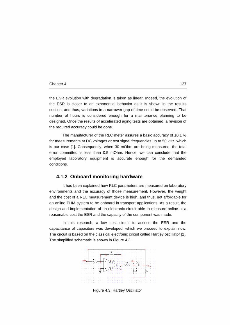
Chapter 4 127

the ESR evolution with degradation is taken as linear. Indeed, the evolution of the ESR is closer to an exponential behavior as it is shown in the results section, and thus, variations in a narrower gap of time could be observed. That number of hours is considered enough for a maintenance planning to be designed. Once the results of accelerated aging tests are obtained, a revision of the required accuracy could be done.

The manufacturer of the RLC meter assures a basic accuracy of ±0.1 % for measurements at DC voltages or test signal frequencies up to 50 kHz, which is our case [1]. Consequently, when 30 mOhm are being measured, the total error committed is less than 0.5 mOhm. Hence, we can conclude that the employed laboratory equipment is accurate enough for the demanded conditions.

4.1.2 Onboard monitoring hardware It has been explained how RLC parameters are measured on laboratory

environments and the accuracy of those measurement. However, the weight and the cost of a RLC measurement device is high, and thus, not affordable for an online PHM system to be onboard in transport applications. As a result, the design and implementation of an electronic circuit able to measure online at a reasonable cost the ESR and the capacity of the component was made.

In this research, a low cost circuit to assess the ESR and the capacitance of capacitors was developed, which we proceed to explain now. The circuit is based on the classical electronic circuit called Hartley oscillator [2]. The simplified schematic is shown in Figure 4.3.

Figure 4.3. Hartley Oscillator

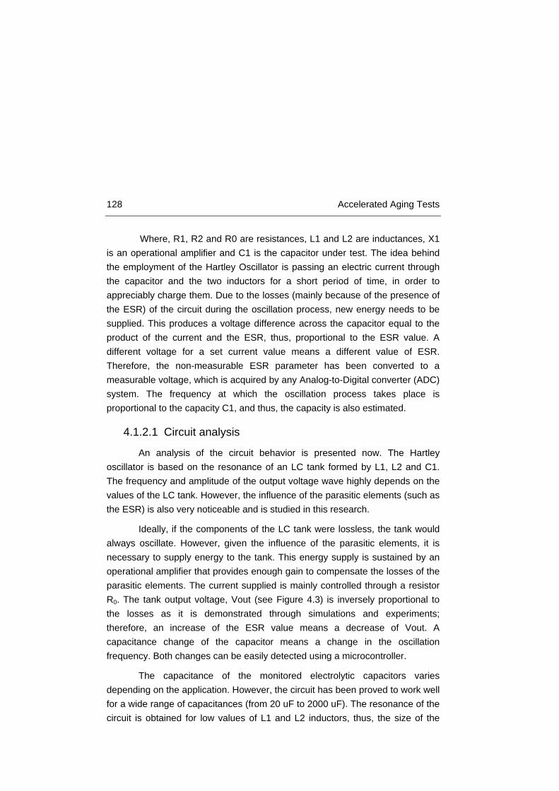
128 Accelerated Aging Tests

Where, R1, R2 and R0 are resistances, L1 and L2 are inductances, X1 is an operational amplifier and C1 is the capacitor under test. The idea behind the employment of the Hartley Oscillator is passing an electric current through the capacitor and the two inductors for a short period of time, in order to appreciably charge them. Due to the losses (mainly because of the presence of the ESR) of the circuit during the oscillation process, new energy needs to be supplied. This produces a voltage difference across the capacitor equal to the product of the current and the ESR, thus, proportional to the ESR value. A different voltage for a set current value means a different value of ESR. Therefore, the non-measurable ESR parameter has been converted to a measurable voltage, which is acquired by any Analog-to-Digital converter (ADC) system. The frequency at which the oscillation process takes place is proportional to the capacity C1, and thus, the capacity is also estimated.

4.1.2.1 Circuit analysis

An analysis of the circuit behavior is presented now. The Hartley oscillator is based on the resonance of an LC tank formed by L1, L2 and C1. The frequency and amplitude of the output voltage wave highly depends on the values of the LC tank. However, the influence of the parasitic elements (such as the ESR) is also very noticeable and is studied in this research.

Ideally, if the components of the LC tank were lossless, the tank would always oscillate. However, given the influence of the parasitic elements, it is necessary to supply energy to the tank. This energy supply is sustained by an operational amplifier that provides enough gain to compensate the losses of the parasitic elements. The current supplied is mainly controlled through a resistor R0. The tank output voltage, Vout (see Figure 4.3) is inversely proportional to the losses as it is demonstrated through simulations and experiments; therefore, an increase of the ESR value means a decrease of Vout. A capacitance change of the capacitor means a change in the oscillation frequency. Both changes can be easily detected using a microcontroller.

The capacitance of the monitored electrolytic capacitors varies depending on the application. However, the circuit has been proved to work well for a wide range of capacitances (from 20 uF to 2000 uF). The resonance of the circuit is obtained for low values of L1 and L2 inductors, thus, the size of the

Chapter 4 129

circuit is kept small. Now, a mathematical analysis of the circuit in Figure 4.3 is done.

4.1.2.1.1 Mathematical analysis

This initial analysis does not consider the parasitic elements of the circuit, and thus, it is an ideal lossless case. The gain of the circuit is provided by the operational amplifier as A = -R2/R1.

Let’s assume Z0 is the equivalent impedance of the parallel of L1 with L2 and C:

𝑍0 = (𝑗𝜔𝐿1)‖ 𝑗𝜔𝐿2 + 1𝑗𝜔𝐶

(Eq. 4.3)

Therefore, VIN is:

𝑉𝐼𝑁 = 𝑍0𝑍0+𝑅0

𝐴𝑉𝑂𝑈𝑇 ≡ 𝐾1𝐴𝑉𝑂𝑈𝑇 (Eq. 4.4)

VIN can also be put as a function of VOUT as:

𝑉𝑂𝑈𝑇 = 𝑍𝐿𝑍𝐿+𝑍𝐶

𝑉𝐼𝑁 ≡ 𝐾2𝑉𝐼𝑁 (Eq. 4.5)

As a result, given Eqs. 4.4 and 4.5, the following expression could be written:

𝑉𝐼𝑁 = 𝐴𝐾1𝐾2 𝑉𝐼𝑁 (Eq. 4.6)

Therefore, the circuit is capable of sustaining the oscillations as long as AK1K2=1. Where, AK1K2 is defined in Eq. 4.7:

𝐴𝐾1𝐾2 = 𝑅2𝑅1

1

−1+ 1𝜔2𝐿2𝐶

−𝑗𝑅0𝜔 ( 1𝜔2𝐿2𝐿1

− 1𝐿2− 1𝐿1

) (Eq. 4.7)

As AK1K2 is a real value, the imaginary part should be zero. So, the resonance frequency can be obtained as:

𝑓0 = 12𝜋𝐶(𝐿1+𝐿2)

(Eq. 4.8)

And the real part determines the minimum gain to sustain the oscillation: 𝑅2𝑅1

𝐿2𝐿1

= 1 (Eq. 4.9)

The previous equations only describe the basic behavior of the circuit for ideal components. However, in this application, it is of paramount importance to understand the behavior of the circuit considering the parasitic

130 Accelerated Aging Tests

elements (the series resistance of the inductors and the ESR). In order to do so, two actions were taken. On the first hand, a detailed mathematical analysis of the circuit was carried out considering the parasitic elements. On the other hand, simulations were run with pSpice.

The transfer function of the circuit was obtained employing the laplace transform. The impedances, assuming null the initial conditions and introducing the parasitic elements are: ZL1=sL1 + RL1; ZL2=sL2 + RL2; ZL1= RC + 1/sC; now, Z0

is assumed:

𝑍0 = (𝑍𝐿1)‖(𝑍𝐿2 + 𝑍𝐶) (Eq. 4.10)

Therefore, the transfer function of the circuit can be obtained from equation 4.6, where AK1K2 = 1.

𝐴𝐾1𝐾2 = −𝑅2𝑅1

∗ 𝑍𝐿1∗(𝑍𝐿2+𝑍𝐶)𝑍𝐿1∗(𝑍𝐿2+𝑍𝐶)+𝑅0∗(𝑍𝐿1+𝑍𝐿2+𝑍𝐶)

∗ 𝑍𝐿2𝑍𝐿2+𝑍𝐶

(Eq. 4.11)

After some little algebra, the following transfer function of the circuit was

obtained:

𝐺(𝑠) =

𝐴 ∗[𝑠𝐶]∗[𝑅𝐿1𝑅𝐿2+𝑠(𝐿1𝑅𝐿2+𝑅𝐿1𝐿2)+𝑠2𝐿1𝐿2]

(𝑅𝑜+𝑅𝐿1)+𝑠(𝐿1+𝐶𝑅𝐿1𝑅𝐶+𝐶𝑅𝐿1𝑅𝐿2+𝐶𝑅0𝑅𝐿1+𝐶𝑅0𝑅𝐿2+𝐶𝑅0𝑅𝐶)+𝑠2(𝐶𝐿1𝑅𝐶+𝐶𝐿2𝑅𝐿1+𝐶𝐿1𝑅𝐿2+𝐶𝑅0𝐿1+𝐶𝑅0𝐿2)+𝑠3𝐶𝐿1𝐿2

(Eq. 4.12)

The behavior of the transfer function observed in eq. 4.12 was analyzed in Matlab, obtaining the following bode plot with the same parameter values considered in the simulations section. It can be observed that the resonance frequency is obtained close to a 1 kHz frequency.

Chapter 4 131

4.1.2.1.2 Simulations

Several simulations were developed in order to assess the circuit behavior and check whether the mathematical analysis was correct. The simulation software is ICAP4 from Intusoft®. The real circuit parameters were introduced in the model. The selected operational amplifier is OPA541.

The parasitic elements considered in the simulations are the ESR of the capacitor and the series resistance of inductors. At the time of the circuit development the final capacitors to be tested had not been selected, and thus, the values of a reference capacitor of 300 uF were employed. In Table 4.1 the values measured with the RLC meter of the considered capacitor are shown, as well as the other important parameters of the circuit.

Figure 4.4. Bode plot of ESR circuit Matlab

132 Accelerated Aging Tests

Name Value Unit

Capacity 300 uF

ESR (Typical) 0.002 Ohm

L1≈L2 47 uH

ESR of L (R7, R8) 0.070 Ohm

Gain(R2/R1) 500k/10k Ohm

R0 5 Ohm

Table 4.1. Simulation component values

The simulation results for the parameters in Table 4.1 of the circuit shown in Figure 4.5, give the waveforms shown in Figure 4.6.

Figure 4.5. Simulation circuit schematic

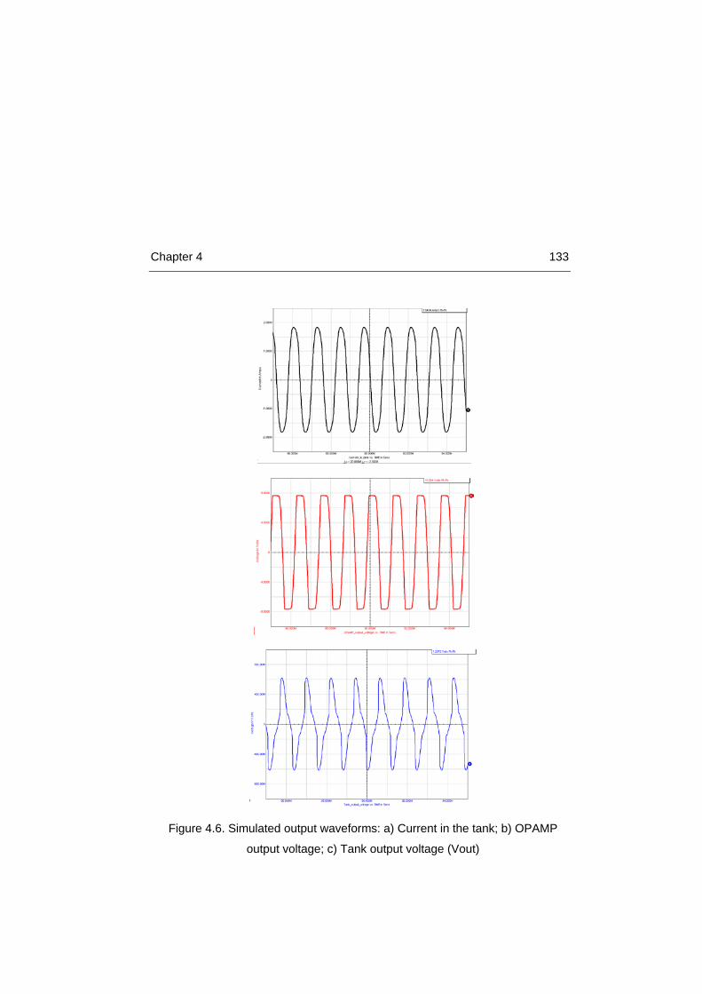
Chapter 4 133

Figure 4.6. Simulated output waveforms: a) Current in the tank; b) OPAMP

output voltage; c) Tank output voltage (Vout)

134 Accelerated Aging Tests

The results of the different simulations can be seen in Table 4.2. The characteristic parameters are: the frequency, the peak to peak current value and the output voltage of the tank (VOUT pk-pk). Notice that a variation of the ESR produces a change in the VOUT pk-pk; a variation in the capacitance produces a change in the oscillation frequency f0.

Simulation 1 2 3 4

Capacitance 300 uF 300uF 300uF 280 uF

ESR 0.002 Ω 0.01 Ω 0.05 Ω 0.002 Ω

f0 800 Hz 800 Hz 775 Hz 862 Hz

Ipk-pk 3.64 A 3.43 A 2.685 A 3.82 A

VOUT pk-pk 1.23 V 1.17 V 923.19 mV 1.34 V

Table 4.2. Simulation results

The simulations proved the following statements:

• An increase of the ESR decreases the output voltage, keeping the frequency almost constant (simulations 1, 2, 3).

• A small decrease in capacity increases the oscillation frequency and the output voltage (simulation 4).

• Once the gain is tuned through R1 and R2, that value is enough to sustain the oscillation for the ESR variation range.

• It is observed that inductors with high values of parasitic resistance reduce the output voltage, and so, the sensibility of the circuit for the variation of capacitor’s ESR is reduced.

• The relationship between the output voltage and the ESR is not strictly linear, but it could be easily approximated and tuned.

Finally, an analysis of the AC transfer characteristic of the circuit was also developed in order to obtain a bode plot with the simulation software. It can be observed that the results from the mathematical analysis (Figure 4.4) and the simulations (Figure 4.7) match.

Chapter 4 135

4.1.2.2 Experimental results

The prototype is shown in Figure 4.10. When the experimental results were developed, the accelerated aging tests have not been done yet, and thus, the ESR was artificially increased through the addition of copper wires. Three copper wires of 8.6 cm, 17 cm and 26 cm length with equivalent series resistances of 70 mΩ, 108 mΩ and 150 mΩ respectively, were used to increase the ESR. The gain of the circuit was set in 60 and R0 in 5 Ohm.

Figure 4.7. Bode plot pSpice simulations

136 Accelerated Aging Tests

The results obtained for the capacitor are shown in the following table:

Experiment 1 2 3 4

Capacity 303 uF 303 uF 303 uF 303 uF

ESR 0.006 Ω 0.07 Ω 0.108 Ω 0.150 Ω

f0 833 Hz 800 Hz 790 Hz 781 Hz

Ipk-pk 3.49 A 2.67 A 2.23 A 1.92 A

VOUT pk-pk 1.10 V 850 mV 710 mV 590 mV

Table 4.3. Results of experiments

The waveforms of the measured signals on the oscilloscope for the experiment of Table 4.3 can be seen on Figure 4.8. The red line is the current in the tank; the yellow line is the input voltage to the tank from the OPA445 operational amplifier and the green line is the output voltage of the tank (VOUT).

It can be seen that the output waveforms of the circuit (Figure 4.8) are very close to the ones predicted by the simulations (Figure 4.6). It must be highlighted the low standard deviation of the measurements, therefore a high

Figure 4.8. Experiments waveforms

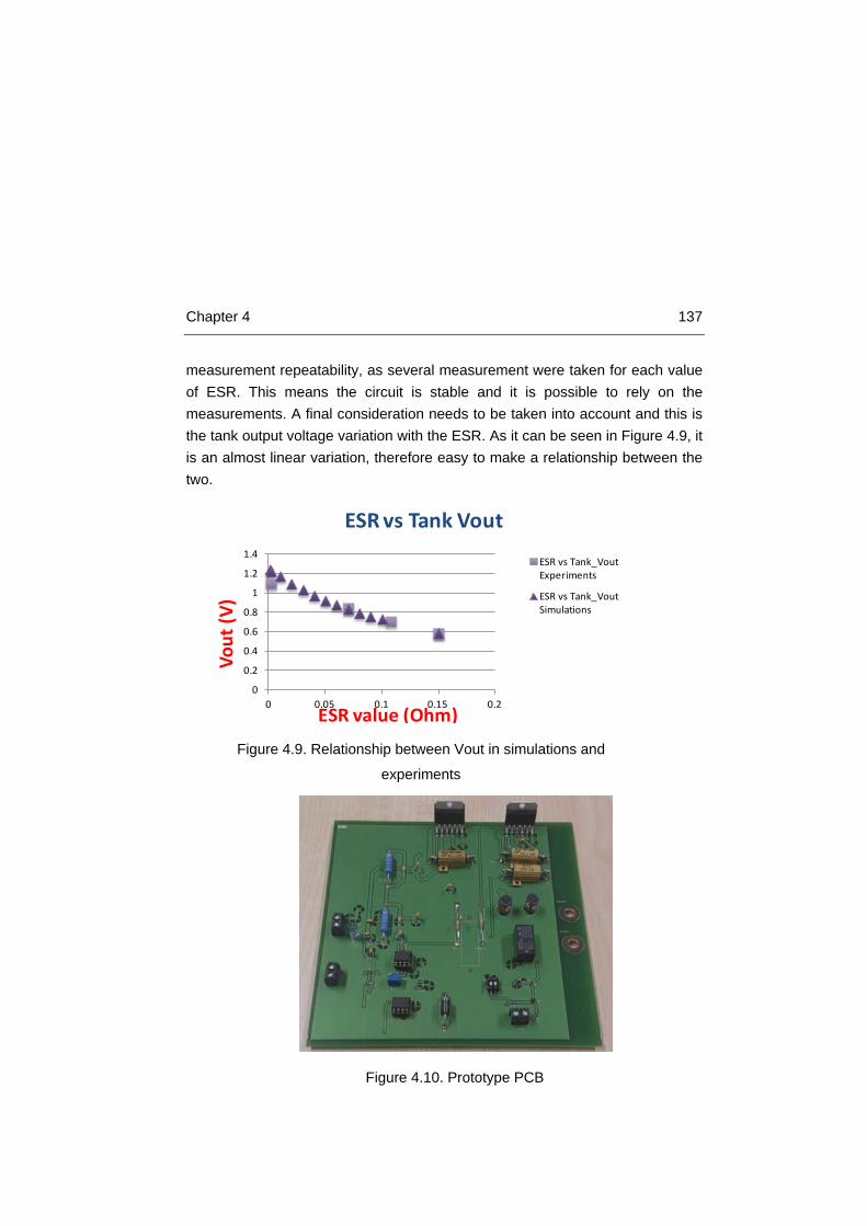
Chapter 4 137

measurement repeatability, as several measurement were taken for each value of ESR. This means the circuit is stable and it is possible to rely on the measurements. A final consideration needs to be taken into account and this is the tank output voltage variation with the ESR. As it can be seen in Figure 4.9, it is an almost linear variation, therefore easy to make a relationship between the two.

Figure 4.10. Prototype PCB

Figure 4.9. Relationship between Vout in simulations and

experiments

0

0.2

0.4

0.6

0.8

1

1.2

1.4

0 0.05 0.1 0.15 0.2

Vout

(V)

ESR value (Ohm)

ESR vs Tank Vout

ESR vs Tank_Vout Experiments

ESR vs Tank_Vout Simulations

138 Accelerated Aging Tests

4.1.2.3 Measurements accuracy

Previously, a desired accuracy of ±1 mOhm had been set for the lab tests. It would be a great monitoring system if that value could be obtained for the online monitoring system. The measurement accuracy of online monitoring systems greatly depends on the selected ADC employed, which is the one evaluating the output voltage level of the system dependent on the ESR.

The results of the experiments developed with the ESR measuring device for online monitoring show a voltage amplitude variation of 7.5 mV/mOhm. During the lab tests it was observed that the series resistance of the inductors had an impact on the previous amplitude variation. The greater the resistances, the losses became higher, and thus, the output voltage variation was much smaller. Consequently, the selection of inductors with small parasitic resistance was a critical point in order to achieve the desired accuracy.

A common ADC of 10 bits on a 5 V variation range has a resolution of 5 V/1023 bits = 4.887 mV/bit. Consequently, the selection of a 10 bit ADC system would be enough to observe variations of 1 mOhm on the ESR of the capacitor. A final consideration should be taken into account with respect to temperature. A deep analysis on the influence of the environmental temperature on the measuring device accuracy was not developed, and thus, it should be carried out prior to a final deployment of the system.

4.1.2.4 Conclusions of capacitor online monitoring system

Knowing that the ESR and the capacitance are precursor parameters of capacitors degradation, a cost effective solution has been given in order to convert them into measurable quantities. The results prove that the measurement accuracy is good enough, in order to take decisions on maintenance actions. The PCB size could be optimized, but it has a small number of components.

In conclusion, this design can be used in portable applications where size and cost are the main issue. Together with a reliable prognostic algorithm the capacitor could be replaced before a faulty event occurs, saving costs and increasing the overall reliability of the system.

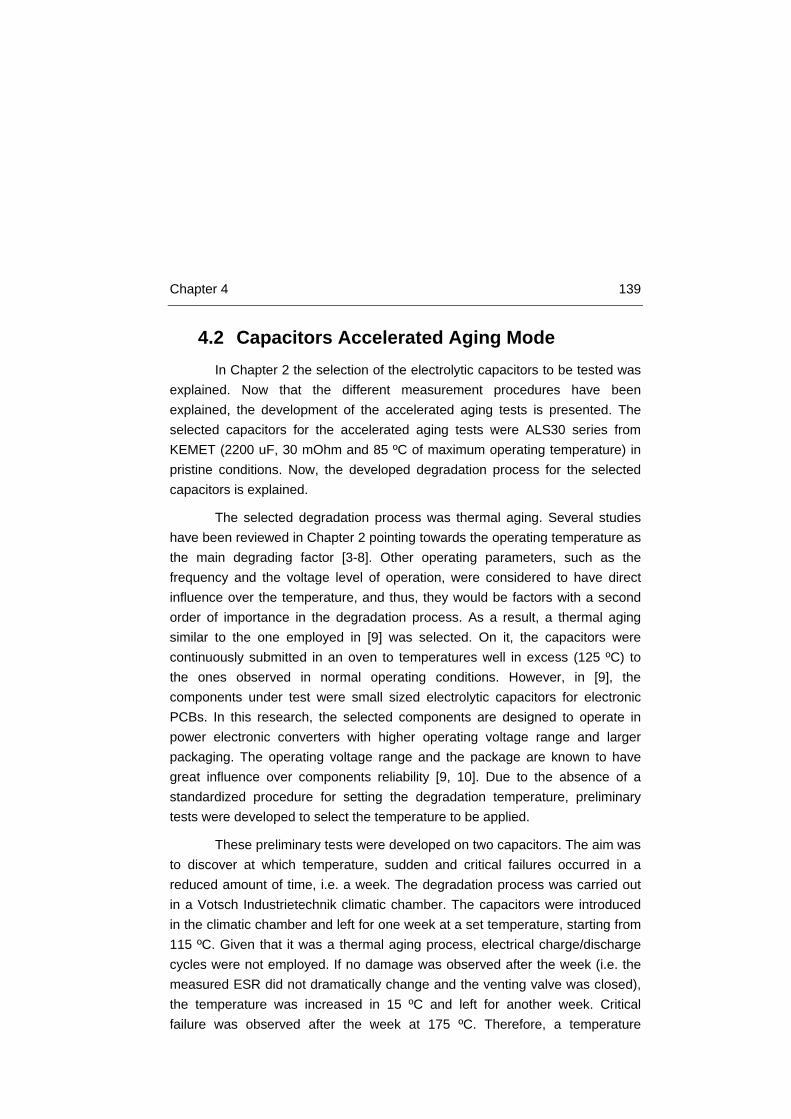
Chapter 4 139

4.2 Capacitors Accelerated Aging Mode In Chapter 2 the selection of the electrolytic capacitors to be tested was

explained. Now that the different measurement procedures have been explained, the development of the accelerated aging tests is presented. The selected capacitors for the accelerated aging tests were ALS30 series from KEMET (2200 uF, 30 mOhm and 85 ºC of maximum operating temperature) in pristine conditions. Now, the developed degradation process for the selected capacitors is explained.

The selected degradation process was thermal aging. Several studies have been reviewed in Chapter 2 pointing towards the operating temperature as the main degrading factor [3-8]. Other operating parameters, such as the frequency and the voltage level of operation, were considered to have direct influence over the temperature, and thus, they would be factors with a second order of importance in the degradation process. As a result, a thermal aging similar to the one employed in [9] was selected. On it, the capacitors were continuously submitted in an oven to temperatures well in excess (125 ºC) to the ones observed in normal operating conditions. However, in [9], the components under test were small sized electrolytic capacitors for electronic PCBs. In this research, the selected components are designed to operate in power electronic converters with higher operating voltage range and larger packaging. The operating voltage range and the package are known to have great influence over components reliability [9, 10]. Due to the absence of a standardized procedure for setting the degradation temperature, preliminary tests were developed to select the temperature to be applied.

These preliminary tests were developed on two capacitors. The aim was to discover at which temperature, sudden and critical failures occurred in a reduced amount of time, i.e. a week. The degradation process was carried out in a Votsch Industrietechnik climatic chamber. The capacitors were introduced in the climatic chamber and left for one week at a set temperature, starting from 115 ºC. Given that it was a thermal aging process, electrical charge/discharge cycles were not employed. If no damage was observed after the week (i.e. the measured ESR did not dramatically change and the venting valve was closed), the temperature was increased in 15 ºC and left for another week. Critical failure was observed after the week at 175 ºC. Therefore, a temperature

140 Accelerated Aging Tests

between 175 ºC and 125 ºC was selected, this is, 145 ºC. With a temperature of 145 ºC, a fast degrading path was assured, while a sudden failure, due to high internal pressure, was avoided.

Two different rounds of test types were developed, one with constant temperatures and another with varying temperatures.

4.2.1 Constant temperature degradation The main characteristic of these accelerated aging tests is that the

temperature of 145 ºC was kept constant during the whole experimental process. Two capacitors were submitted to these experiments.

The experimental test procedure was based on the following steps:

1. Prior to any damaging, components’ parameters in pristine conditions were measured.

2. The capacitors were introduced in the climatic chamber.

3. The temperature was increased in steps of 20 ºC each 10 minutes;

4. Once stationary conditions were reached in the climatic chamber, the components were left for a week at the set constant temperature (145 ºC).

5. After a week, the components were extracted. ESR and capacity measurements were done when the components were at room temperature.

This procedure was repeated from step 2, until components’ ESR value doubled the initial one.

4.2.2 Varying temperature degradation The 2nd round of capacitor degradation through accelerated aging tests

was focused on obtaining experimental data for validation of the prognostic algorithm. Although the constant temperature tests were enough for developing the algorithm, a major contribution of the algorithm is claimed to be the assessment of the degradation of capacitors working under variable operating conditions (Chapter 5). In order to test it, 3 different degradation temperature

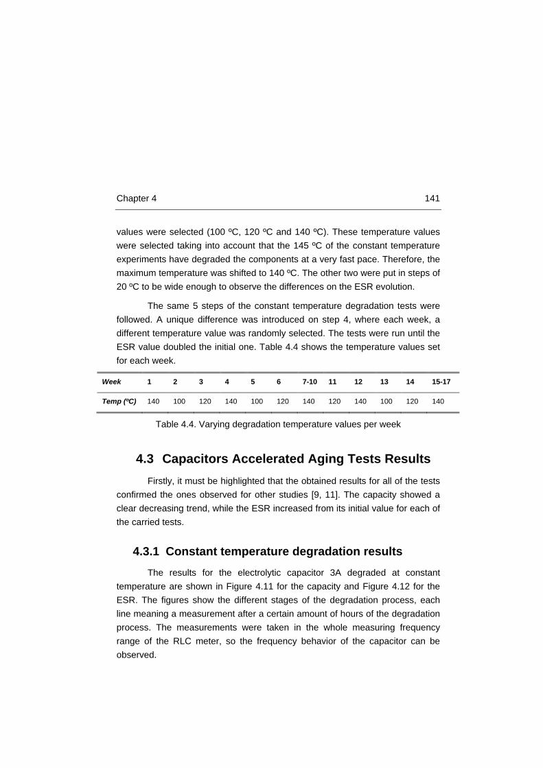
Chapter 4 141

values were selected (100 ºC, 120 ºC and 140 ºC). These temperature values were selected taking into account that the 145 ºC of the constant temperature experiments have degraded the components at a very fast pace. Therefore, the maximum temperature was shifted to 140 ºC. The other two were put in steps of 20 ºC to be wide enough to observe the differences on the ESR evolution.

The same 5 steps of the constant temperature degradation tests were followed. A unique difference was introduced on step 4, where each week, a different temperature value was randomly selected. The tests were run until the ESR value doubled the initial one. Table 4.4 shows the temperature values set for each week.

Week 1 2 3 4 5 6 7-10 11 12 13 14 15-17

Temp (ºC) 140 100 120 140 100 120 140 120 140 100 120 140

Table 4.4. Varying degradation temperature values per week

4.3 Capacitors Accelerated Aging Tests Results Firstly, it must be highlighted that the obtained results for all of the tests

confirmed the ones observed for other studies [9, 11]. The capacity showed a clear decreasing trend, while the ESR increased from its initial value for each of the carried tests.

4.3.1 Constant temperature degradation results The results for the electrolytic capacitor 3A degraded at constant

temperature are shown in Figure 4.11 for the capacity and Figure 4.12 for the ESR. The figures show the different stages of the degradation process, each line meaning a measurement after a certain amount of hours of the degradation process. The measurements were taken in the whole measuring frequency range of the RLC meter, so the frequency behavior of the capacitor can be observed.

142 Accelerated Aging Tests

Figure 4.12. ESR vs- frequency at different degradation cycles

Figure 4.11. Capacity vs frequency at different degradation cycles

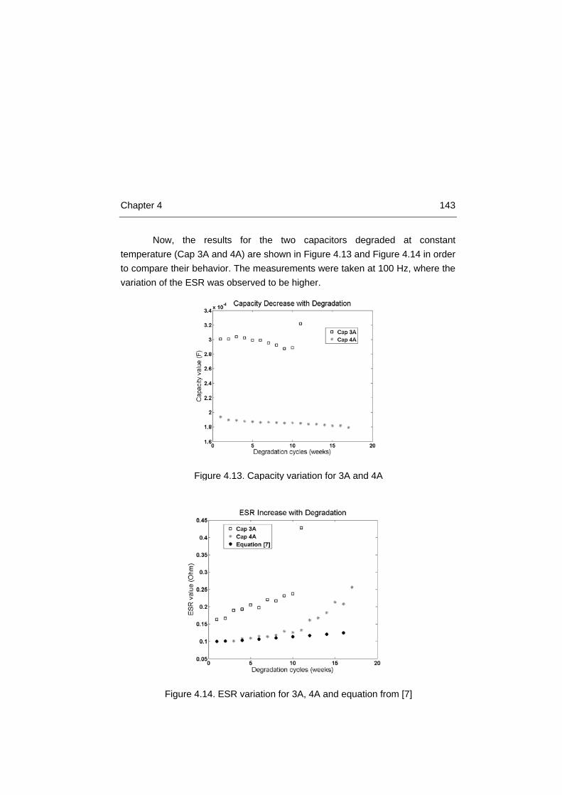
Chapter 4 143

Now, the results for the two capacitors degraded at constant temperature (Cap 3A and 4A) are shown in Figure 4.13 and Figure 4.14 in order to compare their behavior. The measurements were taken at 100 Hz, where the variation of the ESR was observed to be higher.

Figure 4.14. ESR variation for 3A, 4A and equation from [7]

Figure 4.13. Capacity variation for 3A and 4A

144 Accelerated Aging Tests

Following the constant temperature value, the ESR and the capacity showed a constant increasing and decreasing degradation patterns, respectively. The results for a commonly employed equation on model-based prognostics, the model from Abdennaher et al. [8] for the evolution of the ESR, are shown in Figure 4.14 as well. This equation is of vital importance for the development of the prognostic algorithm, thus, the model is deeply revised on Chapter 5, although it is worthy observing the difference of its results with respect to the real degradation curve. The initial ESR value taken for the equation is the same as capacitor 4A. Here, the results of the equation for a constant temperature of 145 ºC are plotted, in order to assess the error on modeling the degradation process of the capacitor. This error needs to be taken into account by the algorithm.

It can be observed that the last measurement of Cap 3A suffered a dramatic change. That capacitor showed great damage after the degradation process (pressure valve opened). It can also be concluded that although the manufacturer claimed that the capacitors had 2200 μF initially, the real measured parameters are slightly different.

4.3.2 Varying temperature degradation results Now, the results for the varying temperature degradation results are

shown. The patterns for all the degraded capacitors are shown in Figure 4.15 and Figure 4.16.

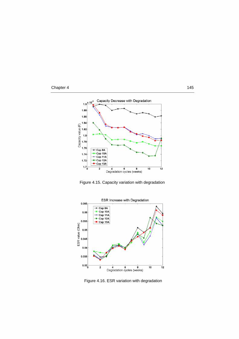
Chapter 4 145

Figure 4.16. ESR variation with degradation

Figure 4.15. Capacity variation with degradation

146 Accelerated Aging Tests

It can be observed that the initial value of the capacity has a wide standard deviation with differences of almost 0.1 mF for capacitors in pristine conditions. It can also be observed that the initial value of 2200 μF claimed by the manufacturer is not reached. It can also be concluded that capacitor 8A and 10A follow the same trend, which slightly differs from the one followed by capacitors 11A, 12A and 13A.

Regarding the ESR, it can be observed that the standard deviation of the initial value is low. It can be also concluded that the patterns of the ESR for the different capacitors are very similar. Therefore, the good prognosticability of the ESR is the most valuable conclusion of these results.

A final test was developed regarding the ESR parameter. The ESR is a parameter known to be temperature dependent. In order to develop the prognostic algorithm, the influence of the temperature in the ESR needs to be known. In particular, ESR was measured at different temperatures on a new capacitor using the FLUKE PM6306 RLC meter in the climatic chamber. The experimental test procedure has been based on the following three steps:

• Setting of the desired temperature in the climatic chamber.

• Once stationary conditions are reached in the climatic chamber, the temperature is maintained for 20 minutes in order to allow the internal layers of the capacitor to heat up and reach the thermodynamic equilibrium with the chamber.

• The ESR is measured.

This procedure has been repeated at 7 different temperatures in the range [15 ºC, 110 ºC], which is expected to be experienced by the capacitor during operation in a FEV.

Therefore, the ESR was measured on a new capacitor for varying thermal conditions. The results of the experiment can be observed on Figure 4.17. It can be observed that the higher the temperature is, the lower the ESR value. This conclusion is provided in other researches [21]. The physical explanation is that for higher temperature values the conductivity of the electrolyte increases, and thus, the ESR decreases.

Chapter 4 147

Figure 4.17 ESR measurement vs Temperature variation

148 Accelerated Aging Tests

4.4 IGBT failure precursor monitoring hardware Similarly to the measurement systems developed for the capacitors

case, for the IGBT two different systems were developed. One was done for lab tests and the other for online monitoring tests.

The circuit designed for lab tests studied IGBT degradation in order to characterize it. The influence of the degradation on the selected preliminary failure precursor parameters needed to be studied. Given the uncertainty of the impact that degradation would have on them, the precision required was high; therefore, tests were run with high accuracy laboratory instruments. From the outcome of these tests, a final set of failure precursor parameters was selected.

The second circuit designed was intended for failure precursor parameter online monitoring. The purpose was to measure the final selected variables under normal operating conditions; this is, during operation of the IGBTs within a real inverter. The online monitoring system was tested with an inverter connected to a resistor load.

Prior to the beginning of the explanation of the measuring hardware the employed failure precursor parameters are recalled:

• Collector-emitter voltage (VCE);

• Collector current (IC);

• Case temperature (TC);

• Gate voltage (VG);

• Gate current (IG).

4.4.1 Laboratory tests measuring hardware It was observed during the literature review on Chapter 3 that the

variation of VCE,ON and VTH due to the degradation was small, in the order of tenths of mV. Therefore, low variation of the signals and possibly low signal-to-noise ratio can be expected. In order to have enough accuracy on the measurements, a minimum resolution of the data acquisition system of 1 mV was set as desired. In this sense, a 16-bit resolution laboratory data acquisition system fulfilling the previous condition was selected: the NI USB-6259 from

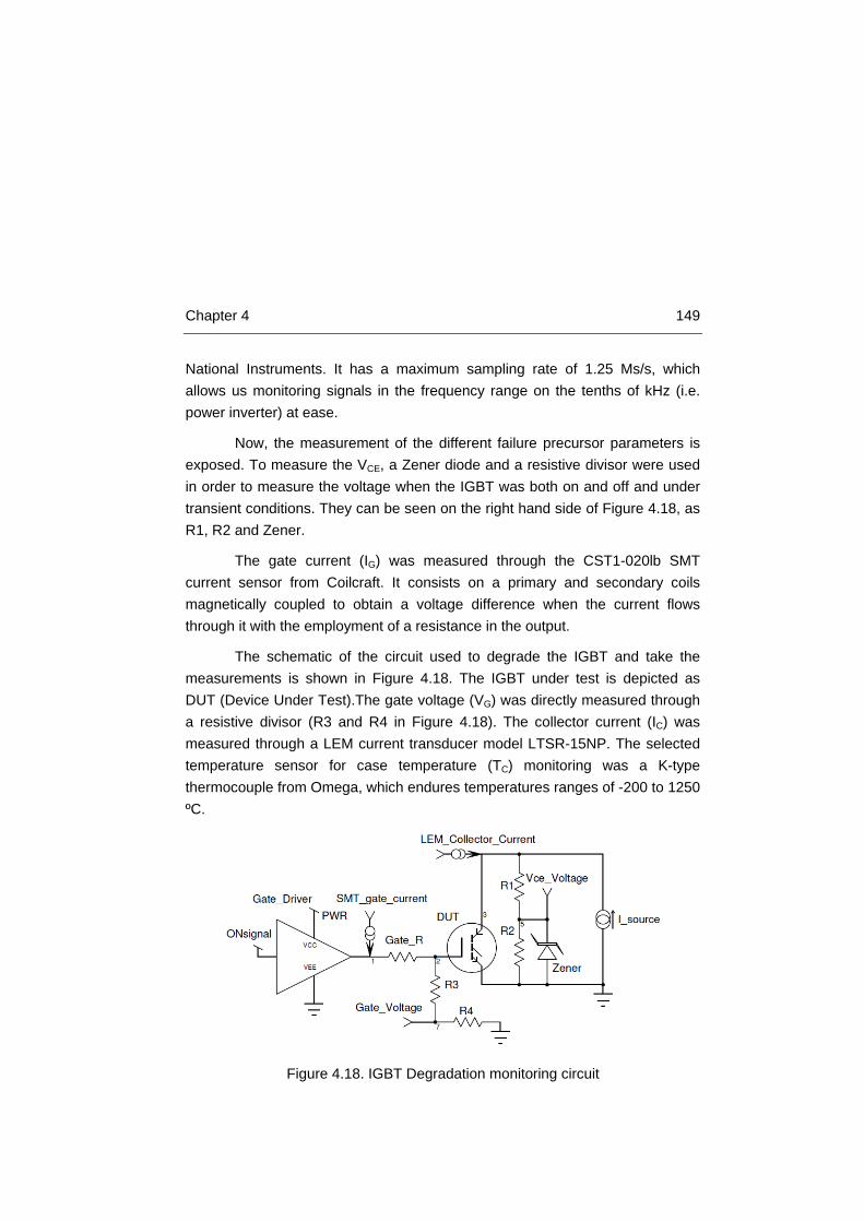
Chapter 4 149

National Instruments. It has a maximum sampling rate of 1.25 Ms/s, which allows us monitoring signals in the frequency range on the tenths of kHz (i.e. power inverter) at ease.

Now, the measurement of the different failure precursor parameters is exposed. To measure the VCE, a Zener diode and a resistive divisor were used in order to measure the voltage when the IGBT was both on and off and under transient conditions. They can be seen on the right hand side of Figure 4.18, as R1, R2 and Zener.

The gate current (IG) was measured through the CST1-020lb SMT current sensor from Coilcraft. It consists on a primary and secondary coils magnetically coupled to obtain a voltage difference when the current flows through it with the employment of a resistance in the output.

The schematic of the circuit used to degrade the IGBT and take the measurements is shown in Figure 4.18. The IGBT under test is depicted as DUT (Device Under Test).The gate voltage (VG) was directly measured through a resistive divisor (R3 and R4 in Figure 4.18). The collector current (IC) was measured through a LEM current transducer model LTSR-15NP. The selected temperature sensor for case temperature (TC) monitoring was a K-type thermocouple from Omega, which endures temperatures ranges of -200 to 1250 ºC.

Figure 4.18. IGBT Degradation monitoring circuit

150 Accelerated Aging Tests

To degrade the IXYS IGBT some modifications to the previous circuit

were required. The IXYS is capable of carrying 110 A in nominal conditions at case temperature of 110 ºC. Given the power limitations of the power supply, 110 A was not reachable, and thus, a resistive divisor at the gate that set the operating conditions in the active region was built. As a result, a power loss of 60 W was dissipated.

4.4.1.1 Measurement accuracy

A critical challenge for the degradation characterization is the measurement accuracy of the signals. A major benefit of the accelerated aging tests, and thus, the lab tests, is that the environment is greatly controlled and the power employed is low. In the accelerated aging tests the highest current flow was 17 A, which limits the electrical noise of the circuits. In this sense, the failure precursor measuring sensors were selected with high accuracy, but small range of measurement.

In lab tests, the accuracy was limited by the data acquisition system, and thus, the measurement error was analyzed on it. Therefore, absolute accuracy for analog inputs was evaluated for the NI USB 6259. A nominal range

Figure 4.19. IGBT degradation Circuit board

Chapter 4 151

of ±5 V was selected to run the calculations. The followed procedure to assess it is established within the component datasheet [12].

Where, Reading = 5 V, GainError = 93 ppm, Range = 5 V, OffsetError = 101 ppm, NoiseUncertainty = 83 μV;

The variables included in Eq. 4.13 receive different values depending on the settings of the data acquisition system, which are included in the component datasheet. The calculations are standardized and so, they are not included here. The outcome of Eq. 4.13 was an absolute accuracy of 1.012 mV. The resolution provided by the manufacturer is 56 μV.

Now, the accuracy of the employed sensors is analyzed. During the accelerated aging tests, the applied on/off switching frequencies was very low, close to DC behavior, taking into account that the on period last around 6 seconds. As a result, the noise that a resistive divisor may produce is negligible, and its accuracy is directly related to the data acquisition system. The LTSR 15-NP current transducer was selected due to its sensitivity of 41.6 mV/A and accuracy of ±0.2 % on full scale, which means an error 0.06 A. Finally, the K-thermocouple sensor adapter device accuracy at full scale is ±1 %, which provides a 3 ºC error.

The range of variation observed in the results for the VCE due to the degradation was in the order of the tenths of mV, which means that the required accuracy needs to be high. According to the obtained results and the analysis of the measured data, it can be concluded that the accuracy of the measuring system was acceptable.

4.4.2 Onboard monitoring hardware A second measurement circuit was built in order to test degraded IGBTs

under normal operating conditions within an inverter, which would replicate the conditions of online monitoring. The aim was to test not only that the selected variables and sensors were appropriate for online prognostics, but also that the measurement procedure was correct and whether it allowed the degradation to

AbsoluteAccuracy = Reading*GainError +

+ Range*OffsetError + Noiseuncertainty (Eq. 4.13)

152 Accelerated Aging Tests

be assessed online. This way, an inverter was also built for testing the degraded components under load.

In this new framework, a sensor system prototype that was closer to what could be integrated in the vehicle for on-board monitoring was developed. This system would also require complying with the features of the PHMS set in Chapter 1. In this sense, the selected variables to be implemented in the final monitoring system would not be the same as the ones selected to monitor in accelerated aging tests. This new selection is a direct consequence of the results observed in the accelerated aging tests, so some of the results are being put forward, but they are later explained.

The final selection of the variables to be monitored in the online system for IGBTs were:

• Collector-emitter voltage (VCE).

• Collector current (IC).

• Case temperature (TC).

In this respect, the VCE, IC and TC measuring sensors, as well as the ADC component were chosen. It must be noted that the measurement resolution within an onboard system, greatly depends on the ADC converter, as it was explained in the capacitors case. During lab tests the data acquisition system from NI was employed, thus, highly reducing the noise of the measurements and improving the accuracy. However, onboard systems employ cheaper and less accurate microcontrollers to collect it. This is an issue to take into account when implementing the final system, as it must be accurate enough to register the minute degradation trends of the parameters.

Another major issue when selecting the components is their power rating. The final inverter employed in a FEV may need to flow powers in the order of kW, and so, the current ratings are larger than in experimental setup. The selected collector-current sensor was a LEM HTFS-200P [13]. There is no connection between the sensor and the power wires, therefore increasing reliability and safety. The output voltage of the sensor ranges from 0 to 5 V.

The temperature sensor used was the same K-Type from OMEGA used in the lab setup. The signal supplied by the sensor needs to be compensated

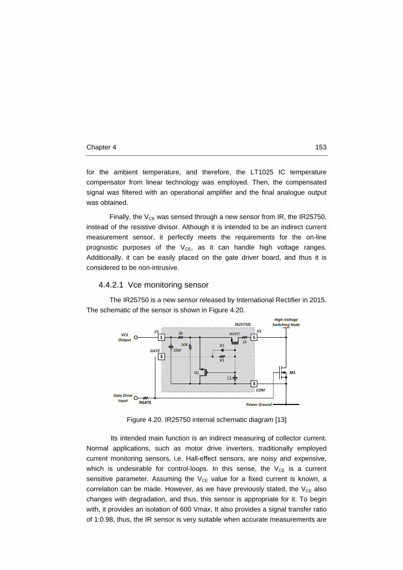
Chapter 4 153

for the ambient temperature, and therefore, the LT1025 IC temperature compensator from linear technology was employed. Then, the compensated signal was filtered with an operational amplifier and the final analogue output was obtained.

Finally, the VCE was sensed through a new sensor from IR, the IR25750, instead of the resistive divisor. Although it is intended to be an indirect current measurement sensor, it perfectly meets the requirements for the on-line prognostic purposes of the VCE, as it can handle high voltage ranges. Additionally, it can be easily placed on the gate driver board, and thus it is considered to be non-intrusive.

4.4.2.1 Vce monitoring sensor

The IR25750 is a new sensor released by International Rectifier in 2015. The schematic of the sensor is shown in Figure 4.20.

Its intended main function is an indirect measuring of collector current. Normal applications, such as motor drive inverters, traditionally employed current monitoring sensors, i.e. Hall-effect sensors, are noisy and expensive, which is undesirable for control-loops. In this sense, the VCE is a current sensitive parameter. Assuming the VCE value for a fixed current is known, a correlation can be made. However, as we have previously stated, the VCE also changes with degradation, and thus, this sensor is appropriate for it. To begin with, it provides an isolation of 600 Vmax. It also provides a signal transfer ratio of 1:0.98, thus, the IR sensor is very suitable when accurate measurements are

Figure 4.20. IR25750 internal schematic diagram [13]

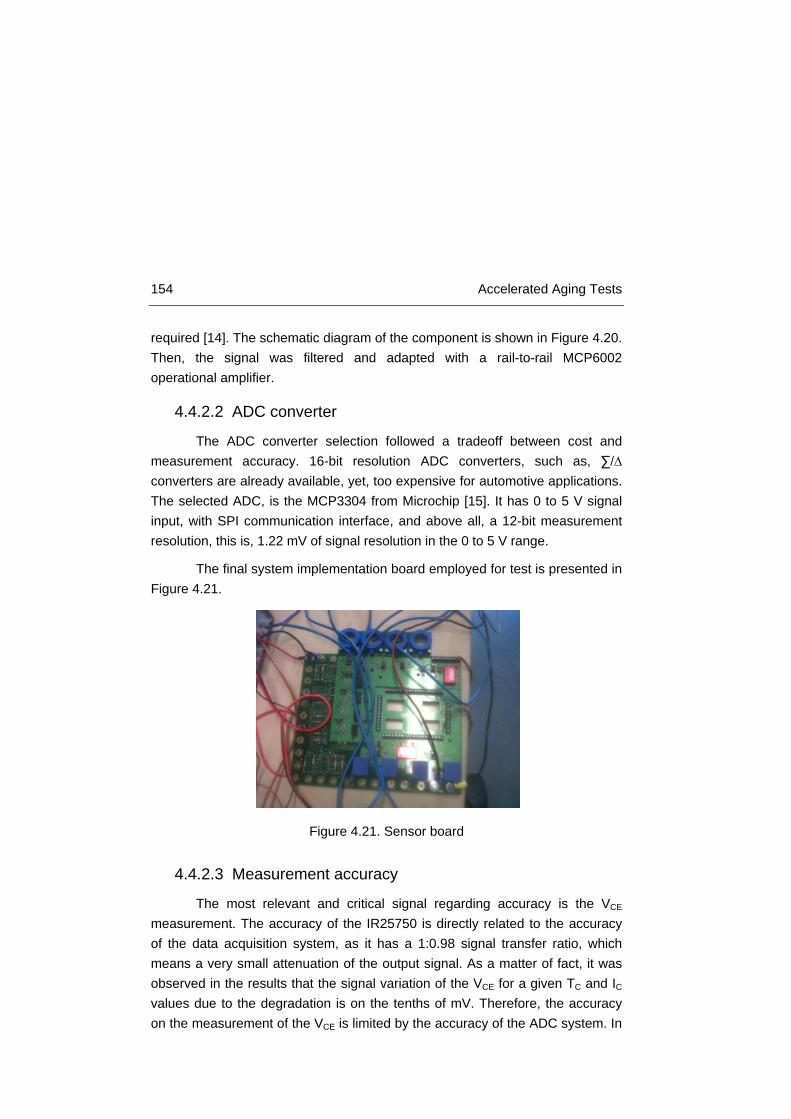
154 Accelerated Aging Tests

required [14]. The schematic diagram of the component is shown in Figure 4.20. Then, the signal was filtered and adapted with a rail-to-rail MCP6002 operational amplifier.

4.4.2.2 ADC converter

The ADC converter selection followed a tradeoff between cost and measurement accuracy. 16-bit resolution ADC converters, such as, ∑/∆ converters are already available, yet, too expensive for automotive applications. The selected ADC, is the MCP3304 from Microchip [15]. It has 0 to 5 V signal input, with SPI communication interface, and above all, a 12-bit measurement resolution, this is, 1.22 mV of signal resolution in the 0 to 5 V range.

The final system implementation board employed for test is presented in Figure 4.21.

4.4.2.3 Measurement accuracy

The most relevant and critical signal regarding accuracy is the VCE measurement. The accuracy of the IR25750 is directly related to the accuracy of the data acquisition system, as it has a 1:0.98 signal transfer ratio, which means a very small attenuation of the output signal. As a matter of fact, it was observed in the results that the signal variation of the VCE for a given TC and IC values due to the degradation is on the tenths of mV. Therefore, the accuracy on the measurement of the VCE is limited by the accuracy of the ADC system. In

Figure 4.21. Sensor board

Chapter 4 155

this sense, the manufacturer of the MCP3304 claims that a maximum error of 6 Least Significant Bits (LSB) could be made on the measurements. This error would mean a maximum deviation of 8 mV for any measurement. The accuracy and error of the measurement system is good enough to be able to detect the signal variations due to the degradation. Nevertheless, given the noisy environment of a FEV powertrain, the fulfillment of the accuracy requirements for the given ADC system should be validated on the final application.

4.5 IGBT Accelerated Aging Tests Mode The selected accelerated aging test mode for IGBT was thermoelectric

degradation process. Several researches suggested its employment for failure mechanism and failure precursor parameter identification [16, 17]. The purpose of thermoelectric degradation process is to increase the junction temperature of the component well above its nominal operating value, in order to accelerate the degrading process. In this process, the component is switched on for a set amount of time while a current flows through it. Due to the power losses generated within the IGBT, its junction temperature raises.

Different application of thermo-electrical degradation processes have been described, some use DC current supply while others apply PWM signals. IGBTs submitted to DC currents endured less number of cycles than the ones with PWM [16], which means that DC current application is more demanding for the IGBT. Given the time constraint at the time of the experiments development and without the observation of any advantage of applying PWM signals, the DC current supply was selected to be applied.

During the accelerated aging tests, 7 IR IGBTs, 5 FUJI IGBTs and 5 IXYS IGBTs were subjected to ageing tests. Each of the selected IGBT types has different maximum junction temperature values. This is due to their manufacturing technologies (see Chapter 3). FUJI and IXYS use newer technology than IR. As previously noticed, the IR IGBTs are PT technology with a TJ,max = 125 ºC and a IC,nom = 16 A. The Trench-FS FUJI can carry the same nominal current with TJ,max = 175 ºC. Finally, the XPT IXYS can carry IC,nom = 110 A with TJ,max = 175 ºC. The IGBT package and design technology had a great influence on the number of lifecycles they can endure [18]. The characteristics of each IGBT type are compiled in Table 4.5.

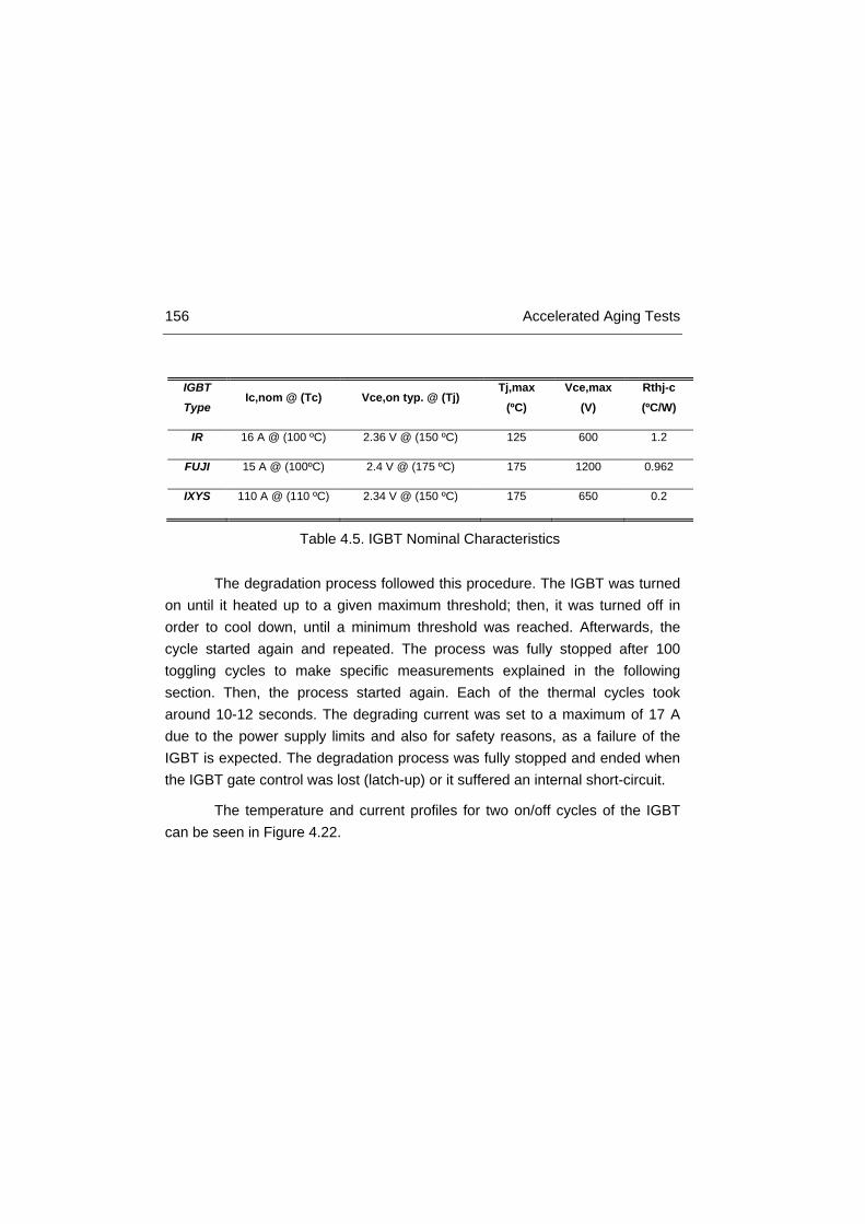
156 Accelerated Aging Tests

The degradation process followed this procedure. The IGBT was turned on until it heated up to a given maximum threshold; then, it was turned off in order to cool down, until a minimum threshold was reached. Afterwards, the cycle started again and repeated. The process was fully stopped after 100 toggling cycles to make specific measurements explained in the following section. Then, the process started again. Each of the thermal cycles took around 10-12 seconds. The degrading current was set to a maximum of 17 A due to the power supply limits and also for safety reasons, as a failure of the IGBT is expected. The degradation process was fully stopped and ended when the IGBT gate control was lost (latch-up) or it suffered an internal short-circuit.

The temperature and current profiles for two on/off cycles of the IGBT can be seen in Figure 4.22.

IGBT Type

Ic,nom @ (Tc) Vce,on typ. @ (Tj) Tj,max

(ºC) Vce,max

(V) Rthj-c (ºC/W)

IR 16 A @ (100 ºC) 2.36 V @ (150 ºC) 125 600 1.2

FUJI 15 A @ (100ºC) 2.4 V @ (175 ºC) 175 1200 0.962

IXYS 110 A @ (110 ºC) 2.34 V @ (150 ºC) 175 650 0.2

Table 4.5. IGBT Nominal Characteristics

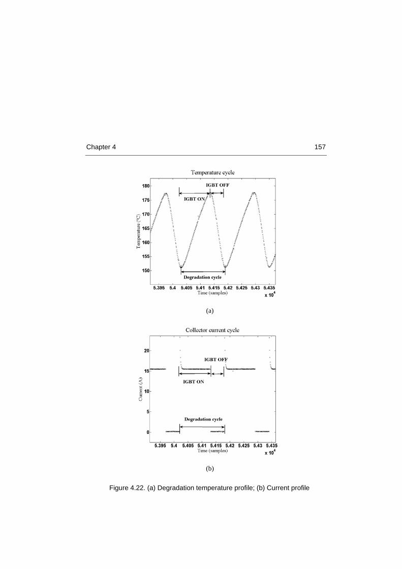
Chapter 4 157

Figure 4.22. (a) Degradation temperature profile; (b) Current profile

(a)

(b)

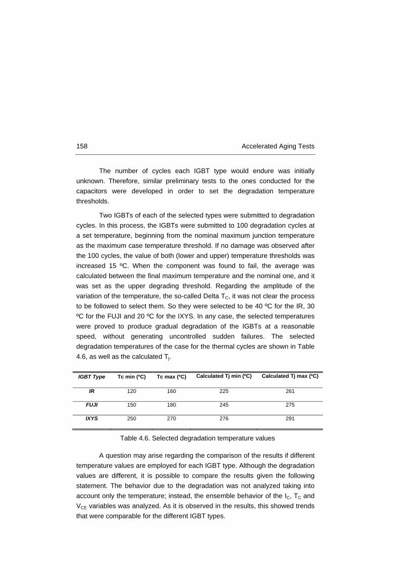
158 Accelerated Aging Tests

The number of cycles each IGBT type would endure was initially unknown. Therefore, similar preliminary tests to the ones conducted for the capacitors were developed in order to set the degradation temperature thresholds.

Two IGBTs of each of the selected types were submitted to degradation cycles. In this process, the IGBTs were submitted to 100 degradation cycles at a set temperature, beginning from the nominal maximum junction temperature as the maximum case temperature threshold. If no damage was observed after the 100 cycles, the value of both (lower and upper) temperature thresholds was increased 15 ºC. When the component was found to fail, the average was calculated between the final maximum temperature and the nominal one, and it was set as the upper degrading threshold. Regarding the amplitude of the variation of the temperature, the so-called Delta TC, it was not clear the process to be followed to select them. So they were selected to be 40 ºC for the IR, 30 ºC for the FUJI and 20 ºC for the IXYS. In any case, the selected temperatures were proved to produce gradual degradation of the IGBTs at a reasonable speed, without generating uncontrolled sudden failures. The selected degradation temperatures of the case for the thermal cycles are shown in Table 4.6, as well as the calculated Tj.

A question may arise regarding the comparison of the results if different temperature values are employed for each IGBT type. Although the degradation values are different, it is possible to compare the results given the following statement. The behavior due to the degradation was not analyzed taking into account only the temperature; instead, the ensemble behavior of the IC, TC and VCE variables was analyzed. As it is observed in the results, this showed trends that were comparable for the different IGBT types.

IGBT Type Tc min (ºC) Tc max (ºC) Calculated Tj min (ºC) Calculated Tj max (ºC)

IR 120 160 225 261

FUJI 150 180 245 275

IXYS 250 270 276 291

Table 4.6. Selected degradation temperature values

Chapter 4 159

Due to time limitations, the IXYS IGBTs were degraded following a continuous process, that is, the degradation process was not stopped every 100 cycles to take measurements. Instead, the measurements were taken at 900 cycles, 1800 cycles and 2700 cycles. This fact is represented in the different shapes of the figures shown in the results for the IXYS IGBTs. After the final measurement at 2700 cycles, the IGBTs were replaced and the degradation was not followed. This procedure was done in order to have IGBTs degraded at different levels but still alive.

Although the failure precursor parameters have been explained, in order to obtain certain measurements, different procedures were followed that are further explained now.

4.5.1 Measurement types Three different measurement types were carried out for the

characterization of the IGBTs: continuous measurements during the degradation process, discrete measurements after each degradation process step (each 100 cycles) and measurements during normal operating conditions in a switching frequency inverter with an ad-hoc designed prototype. They are explained in detail now.

4.5.1.1 Discrete measurements after degradation cycles

After each of the 100 degradation cycles had finished, discrete measurements were taken. These measurements were taken only when the IGBT reached room temperature. The main characteristic of these measurements is that the signals were less noisy and, therefore easier to analyze, and the procedure was controlled and repeatable. There were two types of discrete measurements. On the one hand, the threshold voltage (VGE,TH) was measured. The VGE,TH has been previously defined as the minimum gate voltage (VG) for the IGBT to be considered in the on-state. Therefore, its measurement consisted on slowly increasing the gate voltage until the flowing collector current (IC) value showed a dramatic change, meaning the IGBT is on. During the process, the gate voltage was accurately monitored and recorded. The current supplied to the IGBT was limited to 250 mA in order to keep low the heating rate and the temperature as constant as possible, but big enough to

160 Accelerated Aging Tests

observe the change. The second measurement focused on the VCE,SAT. The VCE,SAT is defined as the VCE value at which the IGBT is in the on state while a set IC flows. The IGBT was switched on for three seconds, letting a fixed current rate of 10 A to flow. The sampling frequency of these measurements was 100 Hz.

4.5.1.2 Continuous measurements during degradation cycles

Continuous degradation measurements of the five variables (IG, VG, IC, TC, VCE) were collected during each of the degradation cycles. Although this kind of measurement is noisy and includes some transient information, it allows the dynamic behavior of IGBTs to be studied for a given collector current and case temperature range. The selected temperature range and collector current values to plot the VCE were:

• IR:

o Tc: 150 and 160 ºC.

o Ic: 15 and 16 A.

• FUJI:

o Tc: 170 and 180 ºC.

o Ic: 15 and 16 A.

• IXYS:

o Tc: 260 and 270 ºC.

o Ic: 14 and 15 A.

This process makes it possible to compare the behavior of the different IGBT types operating under the same conditions. The sampling frequency of the data acquisition system during this process was set to 10 Hz. On the one hand, the selected sampling frequency allows monitoring the degradation behavior with enough detail, which is shown in Figure 4.22. Besides, the size of the data file was small enough to be managed during the data treatment phase.

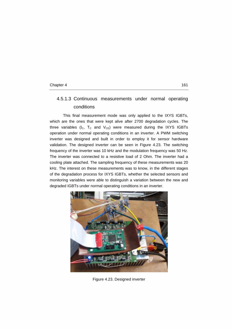
Chapter 4 161

4.5.1.3 Continuous measurements under normal operating

conditions

This final measurement mode was only applied to the IXYS IGBTs, which are the ones that were kept alive after 2700 degradation cycles. The three variables (IC, TC and VCE) were measured during the IXYS IGBTs operation under normal operating conditions in an inverter. A PWM switching inverter was designed and built in order to employ it for sensor hardware validation. The designed inverter can be seen in Figure 4.23. The switching frequency of the inverter was 10 kHz and the modulation frequency was 50 Hz. The inverter was connected to a resistive load of 2 Ohm. The inverter had a cooling plate attached. The sampling frequency of these measurements was 20 kHz. The interest on these measurements was to know, in the different stages of the degradation process for IXYS IGBTs, whether the selected sensors and monitoring variables were able to distinguish a variation between the new and degraded IGBTs under normal operating conditions in an inverter.

Figure 4.23. Designed inverter

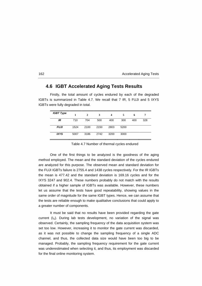
162 Accelerated Aging Tests

4.6 IGBT Accelerated Aging Tests Results Firstly, the total amount of cycles endured by each of the degraded

IGBTs is summarized in Table 4.7. We recall that 7 IR, 5 FUJI and 5 IXYS IGBTs were fully degraded in total.

One of the first things to be analyzed is the goodness of the aging method employed. The mean and the standard deviation of the cycles endured are analyzed for this purpose. The observed mean and standard deviation for the FUJI IGBTs failure is 2755.4 and 1438 cycles respectively. For the IR IGBTs the mean is 477.42 and the standard deviation is 169.16 cycles and for the IXYS 3247 and 902.4. These numbers probably do not match with the results obtained if a higher sample of IGBTs was available. However, these numbers let us assume that the tests have good repeatability, showing values in the same order of magnitude for the same IGBT types. Hence, we can assume that the tests are reliable enough to make qualitative conclusions that could apply to a greater number of components.

It must be said that no results have been provided regarding the gate current (IG). During lab tests development, no variation of the signal was observed. Certainly, the sampling frequency of the data acquisition system was set too low. However, increasing it to monitor the gate current was discarded, as it was not possible to change the sampling frequency of a single ADC channel, and thus, the collected data size would have been too big to be managed. Probably, the sampling frequency requirement for the gate current was underestimated when selecting it, and thus, its employment was discarded for the final online monitoring system.

IGBT Type 1 2 3 4 5 6 7

IR 710 704 500 400 300 400 328

FUJI 1524 2100 2150 2803 5200

IXYS 5007 3186 2742 3200 3000

Table 4.7 Number of thermal cycles endured

Chapter 4 163

The results are now presented. The VGE,TH and VCE,SAT from the discrete measurements are initially shown. Then, the degradation patterns obtained from the continuous measurements during the degradation cycles are presented. In third place, data from continuous measurements under normal operating conditions of IXYS IGBTs in an inverter is shown. Finally, a description of the possible failure mechanisms occurred in the components during the degradation process is provided looking at the inner structure with an optic microscope.

164 Accelerated Aging Tests

Figure 4.24. IGBT threshold voltage for (a) IR, (b) FUJI, (c) IXYS

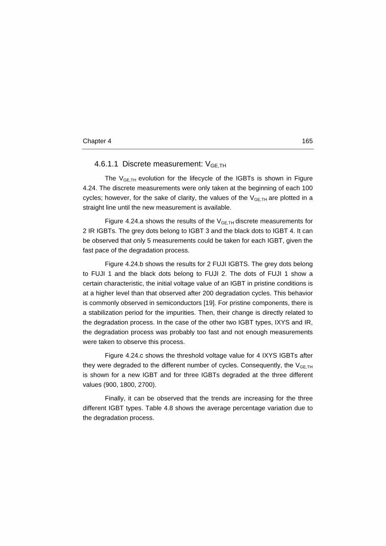
Chapter 4 165

4.6.1.1 Discrete measurement: VGE,TH

The VGE,TH evolution for the lifecycle of the IGBTs is shown in Figure 4.24. The discrete measurements were only taken at the beginning of each 100 cycles; however, for the sake of clarity, the values of the VGE,TH are plotted in a straight line until the new measurement is available.

Figure 4.24.a shows the results of the VGE,TH discrete measurements for 2 IR IGBTs. The grey dots belong to IGBT 3 and the black dots to IGBT 4. It can be observed that only 5 measurements could be taken for each IGBT, given the fast pace of the degradation process.

Figure 4.24.b shows the results for 2 FUJI IGBTS. The grey dots belong to FUJI 1 and the black dots belong to FUJI 2. The dots of FUJI 1 show a certain characteristic, the initial voltage value of an IGBT in pristine conditions is at a higher level than that observed after 200 degradation cycles. This behavior is commonly observed in semiconductors [19]. For pristine components, there is a stabilization period for the impurities. Then, their change is directly related to the degradation process. In the case of the other two IGBT types, IXYS and IR, the degradation process was probably too fast and not enough measurements were taken to observe this process.

Figure 4.24.c shows the threshold voltage value for 4 IXYS IGBTs after they were degraded to the different number of cycles. Consequently, the VGE,TH

is shown for a new IGBT and for three IGBTs degraded at the three different values (900, 1800, 2700).

Finally, it can be observed that the trends are increasing for the three different IGBT types. Table 4.8 shows the average percentage variation due to the degradation process.

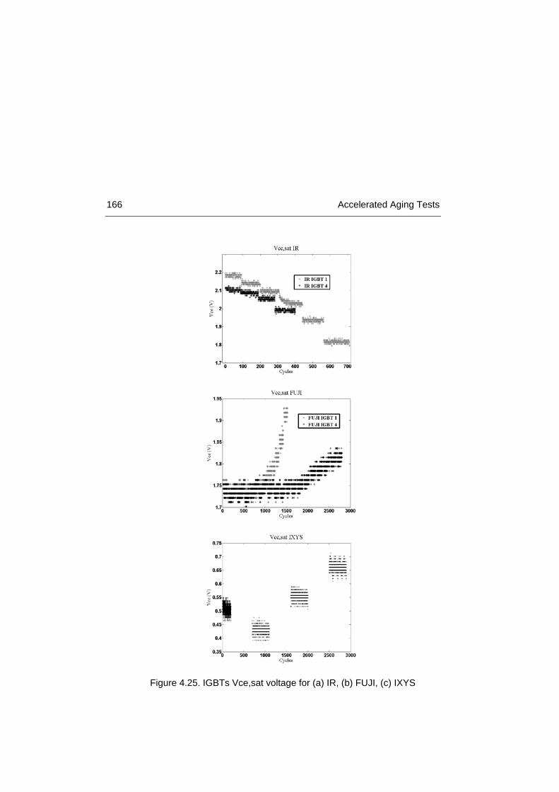
166 Accelerated Aging Tests

Figure 4.25. IGBTs Vce,sat voltage for (a) IR, (b) FUJI, (c) IXYS

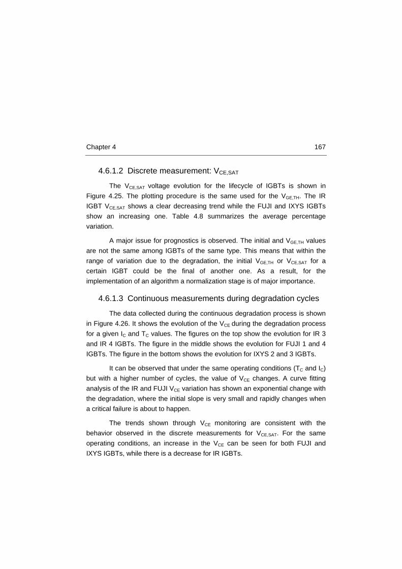
Chapter 4 167

4.6.1.2 Discrete measurement: VCE,SAT

The VCE,SAT voltage evolution for the lifecycle of IGBTs is shown in Figure 4.25. The plotting procedure is the same used for the VGE,TH. The IR IGBT VCE,SAT shows a clear decreasing trend while the FUJI and IXYS IGBTs show an increasing one. Table 4.8 summarizes the average percentage variation.

A major issue for prognostics is observed. The initial and VGE,TH values are not the same among IGBTs of the same type. This means that within the range of variation due to the degradation, the initial VGE,TH or VCE,SAT for a certain IGBT could be the final of another one. As a result, for the implementation of an algorithm a normalization stage is of major importance.

4.6.1.3 Continuous measurements during degradation cycles

The data collected during the continuous degradation process is shown in Figure 4.26. It shows the evolution of the VCE during the degradation process for a given IC and TC values. The figures on the top show the evolution for IR 3 and IR 4 IGBTs. The figure in the middle shows the evolution for FUJI 1 and 4 IGBTs. The figure in the bottom shows the evolution for IXYS 2 and 3 IGBTs.

It can be observed that under the same operating conditions (TC and IC) but with a higher number of cycles, the value of VCE changes. A curve fitting analysis of the IR and FUJI VCE variation has shown an exponential change with the degradation, where the initial slope is very small and rapidly changes when a critical failure is about to happen.

The trends shown through VCE monitoring are consistent with the behavior observed in the discrete measurements for VCE,SAT. For the same operating conditions, an increase in the VCE can be seen for both FUJI and IXYS IGBTs, while there is a decrease for IR IGBTs.

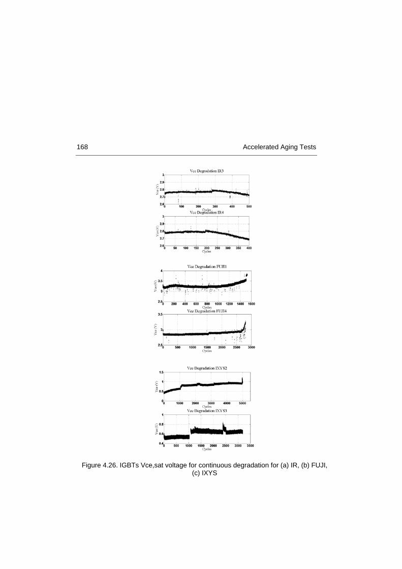
168 Accelerated Aging Tests

Figure 4.26. IGBTs Vce,sat voltage for continuous degradation for (a) IR, (b) FUJI, (c) IXYS

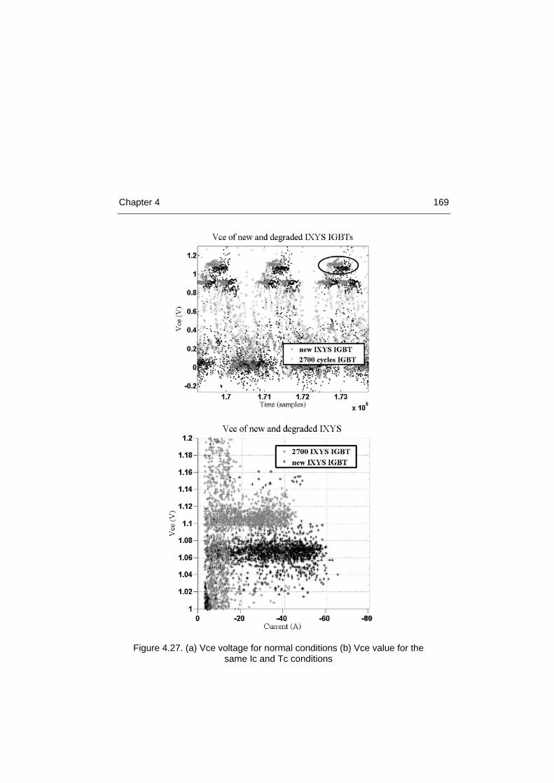
Chapter 4 169

Figure 4.27. (a) Vce voltage for normal conditions (b) Vce value for the same Ic and Tc conditions

170 Accelerated Aging Tests

4.6.1.4 Continuous measurements under normal operating

conditions

Finally, the results obtained for the IXYS IGBTs under normal operating conditions are presented. A new IGBT and a close to end-of-life degraded one (2700 cycles) were tested.

Figure 4.27.a shows the VCE signal during inverter operation for both IGBTs. In the figure, three switching transients can be observed. The grey dots represent the degraded IGBT and the black ones represent the new one.

Figure 4.27.b shows the VCE signal for the new and the degraded one for the same TC operating conditions (30 to 40 ºC). It was observed for the continuous measurements that during the degradation process the VCE value tends to increase. Figure 4.27.b shows this behavior, where the dots of the degraded IGBT are on top of the new one, for a given TC and IC. The average maximum value of the degraded IGBT is 1.105 V, while the new one shows an average of 1.060 V. Therefore, we observe a drift of 40 mV on the VCE signal. It must be highlighted that using the IR25750 VCE sensor along with the current and temperature ones and together with the data acquisition system it was possible to distinguish the variation between the older and the newer IGBT. This shows that if the VCE is measured accurately enough, the degradation can be assessed under normal operating conditions. The measurements were not carried out with the ADC system due to problems with the SPI interface, so testing whether its accuracy is enough is still pending. However, these tests allow observing that the variation of the VCE during the operation on an inverter is possible.

4.6.2 Degradation mechanisms analysis Once the degradation process was over, a destructive analysis of the

components was carried out in order to discover the degradation mechanisms. Given the nature of thermoelectric degradation process, mechanical damage of the IGBTs inner structure was expected, mainly produced by mechanical fatigue and creeping effects of the large thermal cycles. Some of the components were cut, while others were attacked with H2SO4 to discover the metallization state on

Chapter 4 171

the chip surface. Then, the samples were studied with a LEICA optic microscope.

Firstly, the severity of the developed degradation process must be highlighted. Huge damages were observed in the samples as a consequence of the degradation cycles. A first major difference appears when looking at chip thickness. IR wafer thickness is 380 µm, while FUJI is 120 µm and IXYS is 270 µm.

Figure 4.28.a shows the surface of the gate oxide, once the encapsulant was removed. It can be observed that IR IGBTs suffered gate oxide degradation, which explains the increase of VGE,TH. An increase in VGE,TH is related to gate oxide damage due to hot carrier injection resulting in charge trap [9].

Following other studies results [17, 20] and observing Figure 4.28.b and c, it can be concluded that IR degradation mechanism was related to die-attach solder degradation. Crack appearance on chip-solder interface points to die-attach degradation as a main degradation mechanism. Cracks were created at the extremes of the die attach and propagated to the center of the die. Die attach degradation was probably followed by an increase of temperature at the PN junction, increasing the intrinsic carrier concentration as well, concluding with a VCE,SAT decrease.

Other studies concluded that the increase of VCE,SAT in IGBT modules is a consequence of bond-wire lift off [16, 17, 20]. However, after attacking one of the FUJI samples with H2SO4 and looking at Figure 4.28.f, the operation of bond wire lift off failure mechanism was discarded. The attachment of the bond wires showed full contact.

Observing Figure 4.28.d and e related to FUJI IGBTs, a great destruction of the chip was discovered. It included void and crack propagation on the die attach as well. Similar cracks were observed on IXYS IGBTs. It was concluded that the destruction on the die attach increased the conduction resistance and therefore, the VCE,SAT increased for a given current value. This effect demonstrated to have more importance on FUJI and IXYS IGBTs than the effect of intrinsic carrier concentration, as explained for IR IGBTs case. It

172 Accelerated Aging Tests

can be concluded that the thermo-mechanical fatigue stress induced on the die attach was the main degradation mechanism.

4.6.3 IGBT Accelerated Aging Tests Results Summary First of all, conclusions on the selected failure precursor parameters are

analyzed. To begin with, the selection of the triplet formed by IC, TC and VCE variables have demonstrated to sensibly change due to the degradation of IGBTs when measured together with enough accuracy. The sensor and data acquisition system selection were proved to be able to identify the degradation of IGBTs as well. The employment of the discrete measurements of VCE,SAT and VTH were also valuable for identifying IGBT degradation, so their employment is encouraged. As a result, the gate voltage monitoring (VG) under certain conditions have been proved to be useful. However, in order to measure it, a different procedure from just measuring the operating conditions during normal operation is required, therefore, its implementation in the final measuring system for online monitoring was not done. The IAP also discouraged the employment of this variable.

A positive conclusion of the research is the similar results that have been obtained compared to [17]. IR IGBTs were selected in order to verify that the followed degradation methodology was correct and that the results were reliable. In this sense, similar degradation trends and behavior of the signals were observed when compared to the results of [17].

Finally, a summary extracted from the results is shown in Table 4.8. The percentage variation of the variables due to the degradation process is shown. The main degradation mechanisms and their consequences are presented as well. Finally, the physical damages observed through optic microscopic inspection are included.

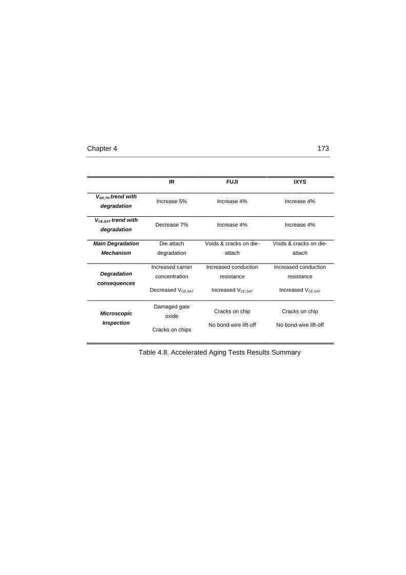
Chapter 4 173

IR FUJI IXYS

VGE,TH trend with degradation

Increase 5% Increase 4% Increase 4%

VCE,SAT trend with degradation

Decrease 7% Increase 4% Increase 4%

Main Degradation Mechanism

Die attach

degradation

Voids & cracks on die-

attach

Voids & cracks on die-

attach

Degradation consequences

Increased carrier

concentration

Decreased VCE,SAT

Increased conduction

resistance

Increased VCE,SAT

Increased conduction

resistance

Increased VCE,SAT

Microscopic Inspection

Damaged gate

oxide

Cracks on chips

Cracks on chip

No bond-wire lift-off

Cracks on chip

No bond-wire lift-off

Table 4.8. Accelerated Aging Tests Results Summary

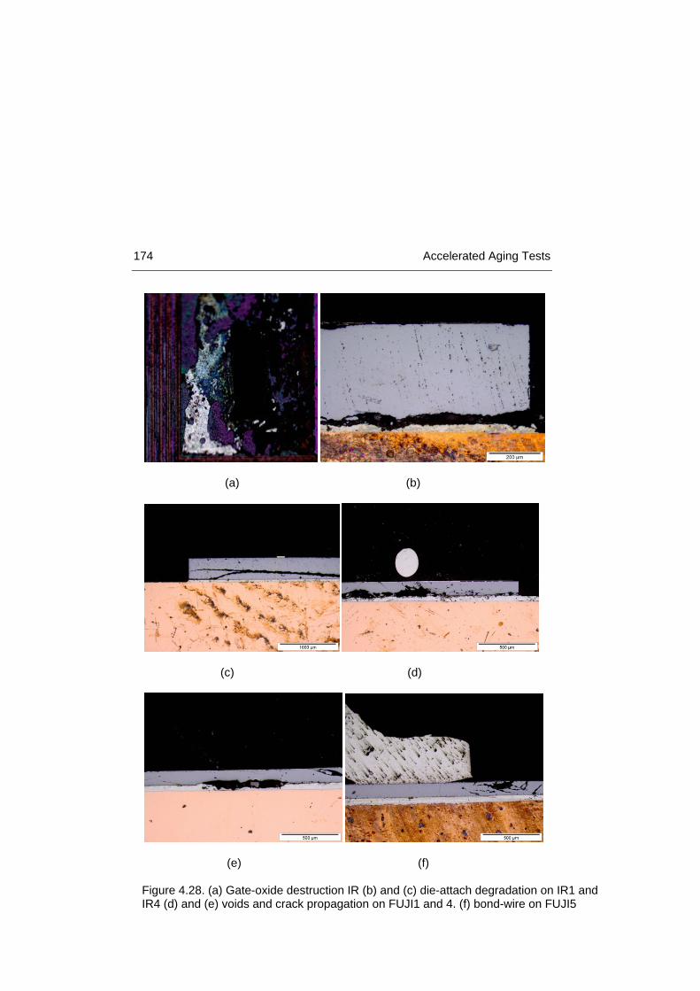
174 Accelerated Aging Tests

(a) (b)

(c) (d)

(e) (f)

Figure 4.28. (a) Gate-oxide destruction IR (b) and (c) die-attach degradation on IR1 and IR4 (d) and (e) voids and crack propagation on FUJI1 and 4. (f) bond-wire on FUJI5

Chapter 4 175

4.7 Accelerated Aging Tests Conclusions In this Chapter, taking into account the failure precursor parameters

reviewed in Chapter 3, they were analyzed through the development of accelerated aging tests. The hardware required in order to monitor them, both in lab tests and online monitoring tests was presented. The required accuracy for the measurements was also provided and stated for each of the cases.

The behavior and the degradation patterns of the failure precursor parameters were presented in the results of the degradation process. Evidences were provided on the IGBT case for the degradation modes and mechanisms.

In the next Chapter, the development of the prognostic algorithms for RUL prediction of components is explained. The results and the data collected during the development of the accelerated aging tests are demonstrated to be of vital importance.

176 Accelerated Aging Tests

4.8 References [1] Programmable Automatic RLC meter PM 6306. User Manual. February,1999

[2] J. Celaya, P. Wysocki, V. Vashchenko, S. Saha and K. Goebel;, "Accelerated aging system for prognostics of power semiconductor devices," AUTOTESTCON, 2010 IEEE, pp. 1, 2010

[3] M. Hao, and L. Wang, “Fault diagnosis and failure prediction of aluminum electrolytic capacitors in power electronic converters, Industrial Electronics Society,” IECON 2005, 31st Annual Conference of IEEE, pp. 6, 2005

[4] A. Braham, A. Lahyani, P. Venet, N. Rejeb, “Recent developments in fault detection and power loss estimation of electrolytic capacitors,” in Power Electronics, IEEE Transactions on, vol. 25, pp. 33-43, 2010

[5] M.A. Vogelsberger, T. Wiesinger and H. Ertl, “Life-cycle monitoring and voltage-managing unit for DC-link electrolytic capacitors in PWM converters,” in Power Electronics, IEEE Transactions on, vol. 26, pp. 493-503, 2011

[6] P. Venet, H. Darnand, and G. Grellet, “Detection of faults of filter capacitors in a converter,” Application to predictive maintenance, in Proceedings International Telecommunications Energy Conference, pp. 229–234.74, 1993

[7] F. Perisse, P. Venet, G. Rojat, and J.M. Rétif, “Simple model of an electrolytic capacitor taking into account the temperature and aging time,” Electrical Engineering, vol. 88, pp. 89-95, 2006

[8] K. Abdennadher, P. Venet, G. Rojat, J.M. Rétif and C. Rosset, “A real-time predictive-maintenance system of aluminum electrolytic capacitors used in uninterrupted power supplies,” in Industry Applications, IEEE Transactions on, vol. 46, pp. 1644-1652, 2010

[9] J. Celaya, C. Kulkarni, S. Saha, G. Biswas, K. Goebel; "Accelerated aging in electrolytic capacitors for prognostics," Reliability and Maintainability Symposium (RAMS), 2012 Proceedings - Annual, pp. 1. 2012

Chapter 4 177

[10] ALS30 series datasheet. Available on: http://www.kemet.com/Lists/ProductCatalog/Attachments/389/KEM_A4031_ALS30_31.pdf

[11] M.L. Gasperi, “Life prediction model for aluminum electrolytic capacitors,” Conference Record - IAS Annual Meeting, IEEE Industry Applications Society, vol. 3, pp. 1347-1351, 1996

[12] Datasheet NI-USB-6259. http://www.ni.com/datasheet/pdf/en/ds-20

[13] LEM HTFS-200P, (2001) (online) Available at: http://www.farnell.com/datasheets/1524365.pdf

[14] IR25730 datasheet (2015) (Online). Available at: http://www.irf.com/product-info/datasheets/data/ir25750lpbf.pdf

[15] MCP3304, (2008), (online) Available at: http://ww1.microchip.com/downloads/en/DeviceDoc/21697e.pdf

[16] V. Smet, F. Forest, J. Huselstein, F. Richardeau, Z. Khatir, S. Lefebvre, M. Berkani;, "Ageing and Failure Modes of IGBT Modules in High-Temperature Power Cycling," Industrial Electronics, IEEE Transactions on, vol. 58, no. 10, pp. 4931-4941, 2011

[17] N. Patil, J. Celaya, D. Das, K. Goebel and M. Pecht;, "Precursor Parameter Identification for Insulated Gate Bipolar Transistor (IGBT) Prognostics," in Reliability, IEEE Transactions on, vol.58, no.2, pp.271-276, June 2009

[18] R. Bayerer, T. Herrmann, T. Licht, J. Lutz and M. Feller, "Model for Power Cycling lifetime of IGBT Modules: various factors influencing lifetime," Integrated Power Systems (CIPS), 2008 5th International Conference on VDE, pp. 1, 2008

[19] A. Christou, W.M. Webb; “Reliability of Compound Analogue Semiconductor Integrated Circuits,” RIAC, 2006

[20] H. Oh, B. Han, P. McCluskey, C. Han, B.D. Youn, "Physics-of-Failure, Condition Monitoring and Prognostics of Insulated Gate Bipolar Transistor

178 Accelerated Aging Tests

Modules: A Review," in Power Electronics, IEEE Transactions on, vol. 30, pp. 2413-2426, 2015

[21] E.C Aeloíza, J-H. Kim, P. Ruminot, P.N. Enjeti; “A real Time Method to Estimate Electrolytic Capacitor Condition in PWM Adjustable Speed Drives and Uninterruptible Power Systems,” in Power Electronics Specialists Conference, PESC’05. IEEE 36th, pp. 2867-2872, 2005

Chapter 5

5 Prognostic Algorithms

In the previous chapter, the development and the results of the accelerated aging tests have been analyzed. The sensors and hardware to be employed have been described, enabling the collection of accurate data. The failure mechanisms and failure precursor parameters have been identified. Moreover, valuable data of components degradation process have been collected. Consequently, on the way for a PHMS implementation, enough data and information are available to proceed with the development of the prognostic algorithms in order to predict the RUL and the health state of the degrading components.

Prognostics of failures in equipment is based on the capability of predicting future degradation paths, so as to estimate the Remaining Useful Life (RUL) of the equipment and the potential risks associated to its failure [1]. On this basis, it is possible to define predictive maintenance strategies to set the best maintenance actions for allowing the optimal exploitation of the useful life of the monitored equipment, with benefits in terms of reduction of costs and improvement of safety.

On this Chapter, the development and implementation of the prognostic algorithms will be explained. The algorithms will be validated with data collected in accelerated aging tests.

180 Prognostic Algorithms

A special mention must be cited prior to the explanation of prognostic algorithms. The prognostic algorithm for electrolytic capacitor RUL estimation, in which the author cooperated, was designed and implemented by Marco M. Rigamonti within the Nuclear Energy Department of Politecnico di Milano. Besides, during the stay of the author in Politecnico di Milano, the development of the prognostic algorithm for IGBT RUL estimation was guided and supervised by Prof. Piero Baraldi and Prof. Enrico Zio.

5.1 RUL Prediction of Capacitors The objective of the present Chapter is to provide a method for the

prediction of the RUL for a capacitor working in variable operating conditions. The method should also allow estimating the uncertainty affecting the RUL prediction. A complete literature review was presented in Chapter 2 regarding electrolytic capacitor prognosis. However, some of the most relevant conclusions will be revised here.

Major issues were found during the literature review regarding prognosis of electrolytic capacitors. Among them, the following three points were concluded:

• The previous prognostic algorithms cannot cope with variable operating conditions and abrupt changes of the degradation parameters.

• The effect of temperature on ESR measurements is not considered.

• The predictions are not supplied with any uncertainty boundary.

However, previous investigations proved useful models of components degradation process with close relationship to the physical effect taking place on real applications. Regarding the information and the models available on electrolytic capacitors degradation the employment of a model-based rather than a data-driven approach is suggested. Consequently, in this work, a model-based prognostic approach will be employed, which uses mathematical representations of the degradation process to predict the RUL of components.

In model-based prognostics, it is possible to distinguish between two different situations: i) the effects of operating conditions on the degradation

Chapter 5 181

process and on the measured signals are known and represented in the mathematical models, ii) the effects are not fully known and a mathematical model of the operating conditions influence is not available. In the former situation i), traditional model-based prognostic approaches, such as those based on Bayesian Filters [2], can be directly used, whereas in the latter ii) properly tailored prognostic approaches must be developed. As it was shown in Chapter 2, Kalman Filters (KF) have been employed in other researches despite of their limitations. In this work, the employment of a sequential Bayesian approach was decided, which is able to deal with the described uncertainties of type ii) and overcome the limitations of KF.

The two main novelties of the proposed prognostic method are:

• the implementation and application to electrolytic capacitors of a particle filtering approach for RUL uncertainty estimation.

• the definition of a novel degradation indicator for capacitors operating at variable temperatures.

In order to take into account the temperature at which the ESR measurements are taken, and thus, to make the prognostic algorithm independent of it, a new degradation indicator was developed. The proposed degradation indicator is the ratio between the ESR measured on the degraded capacitor and the ESR value expected on a new capacitor at the same operational temperature. This index provides an indication of the capacitor degradation level and, since it is independent from the measurement temperature, it can be used for capacitors working in variable operating conditions. Its definition has required performing a series of laboratory experiments for investigating the relationship between the ESR and the temperature in a new capacitor, which have been explained in Chapter 4.

The physics-based model of the ESR evolution proposed in [3], has been applied to the new degradation indicator and used within a sequential Bayesian approach for the estimation of component degradation. The Bayesian approach has been employed to account for the uncertainty affecting: i) the ESR and temperature measurement processes, ii) the possible inaccuracy of the degradation model (see Chapter 4.3.1), iii) the stochasticity of the degradation process. These sources of uncertainty cannot be modeled as

182 Prognostic Algorithms

additive noises, since it is not expected them to be normally distributed in the time domain (Gaussian noise). Therefore, a classical Kalman Filter approach cannot be applied to this problem due to the presence of non-additive noise terms. Consequently, we resort to a Particle Filtering (PF) approach which is able to deal with non-additive noise terms [4]. Once the component degradation state probability distribution has been estimated by the PF method, Monte Carlo (MC) simulation has been used for the prediction of the future component degradation path and its RUL [5]. The MC simulation allows to properly take into account the uncertainty on the present degradation state estimation and the uncertainty on the future evolution of the operating conditions.

The performance of the proposed prognostic method will be verified with respect to the degradation data collected in laboratory accelerated aging tests.

5.1.1 Particle filter-based prognostics theory It is considered a situation in which a physics-based model of the

degradation process is available and can be formulated in the form of a first-order Markov Process:

( )11 , −−= ttt xgx γ (Eq. 5.1)

Where 𝑔(𝑥, 𝛾) is a recursive, possibly non-linear, transition function, 𝑥𝑡 is the indicator of the equipment degradation state at time t and 𝛾 is the process noise used to capture the degradation process stochasticity and the inaccuracy of the model.

It is assumed that the observation equation providing a link between the degradation state x and its measures is known and can be represented by a possibly non-linear function h:

( )ttt xhz σ,= (Eq. 5.2)

Where, σ is the noise of the measurement. The PF-based approach to prognostics relies on the following three steps (Figure 5.1):

1. A filtering step for the estimation of the equipment degradation state at the present time, which is based on the use of Eqs. (5.1) and (5.2) and the measures, z1:t, performed until the present time.

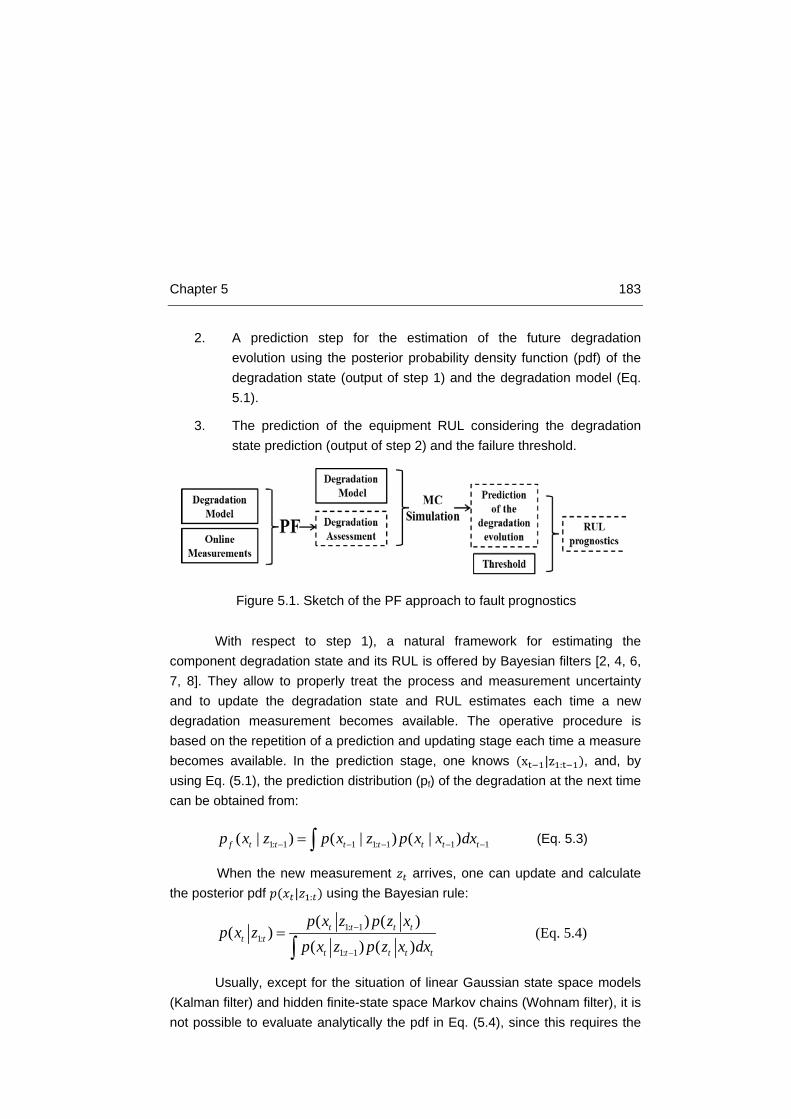
Chapter 5 183

2. A prediction step for the estimation of the future degradation evolution using the posterior probability density function (pdf) of the degradation state (output of step 1) and the degradation model (Eq. 5.1).

3. The prediction of the equipment RUL considering the degradation state prediction (output of step 2) and the failure threshold.

With respect to step 1), a natural framework for estimating the component degradation state and its RUL is offered by Bayesian filters [2, 4, 6, 7, 8]. They allow to properly treat the process and measurement uncertainty and to update the degradation state and RUL estimates each time a new degradation measurement becomes available. The operative procedure is based on the repetition of a prediction and updating stage each time a measure becomes available. In the prediction stage, one knows (xt−1|z1:t−1), and, by using Eq. (5.1), the prediction distribution (pf) of the degradation at the next time can be obtained from:

1: 1 1 1: 1 1 1( | ) ( | ) ( | )f t t t t t t tp x z p x z p x x dx− − − − −= ∫ (Eq. 5.3)

When the new measurement 𝑧𝑡 arrives, one can update and calculate the posterior pdf 𝑝(𝑥𝑡|𝑧1:𝑡) using the Bayesian rule:

1: 11:

1: 1

( ) ( )( )

( ) ( )t t t t

t tt t t t t

p x z p z xp x z

p x z p z x dx−

−

=∫

(Eq. 5.4)

Usually, except for the situation of linear Gaussian state space models (Kalman filter) and hidden finite-state space Markov chains (Wohnam filter), it is not possible to evaluate analytically the pdf in Eq. (5.4), since this requires the

Figure 5.1. Sketch of the PF approach to fault prognostics

184 Prognostic Algorithms

calculation of complex high-dimensional integrals. Particle Filter (PF) provides a numerical solution of the degradation state probability, which can be applied in the case of non-linear degradation models and non-Gaussian non-additive noises. The PF solution is based on the Monte Carlo sampling of a large number of samples (called particles) from a proposal pdf (𝑥𝑡|𝑧1:𝑡). Then, the estimated posterior pdf 𝑝𝑒(𝑥𝑡|𝑧1:𝑡) is approximated by:

( )1:1

( )N

i ie t t t t t

ip x z w x xδ

=

≈ −∑ (Eq. 5.5)

Where 𝑥𝑡𝑖(𝑖 = 1,2, … ,𝑁) are the particles sampled from 𝑞(𝑥𝑡|𝑧1:𝑡) and 𝑤𝑡𝑖 is the weight associated to the particle 𝑥𝑡 given by:

( ) ( ))(

':1:0

:0:0:1

ti

t

it

itti

t zxqxpxzp

w = (Eq. 5.6)

One of the most adopted choices is to consider the proposal pdf 𝑞(𝑥𝑡|𝑧1:𝑡) as the transition function, namely 𝑞(𝑥𝑡|𝑧1:𝑡) = 𝑝(𝑥𝑡|𝑥𝑡−1). In this way, using (Eq. 5.7), the particle weights 𝜔𝑡 at time t are provided by:

( )1

1

; i

i i i i tt t t t t N

it

i

ww w p z x ww

−

=

′′ ′= =

′∑ (Eq. 5.7)

Where 𝑝(𝑧𝑡|𝑥𝑡𝑖) is called the likelihood of measurement 𝑧𝑡 given the particle 𝑥𝑡𝑖, which can be derived from the observation function in Eq. (5.2). The reader interested in a detailed description of the PF method for the estimation of the degradation state can refer to [4, 9, 10, 11, 12].

With respect to step 2), once the posterior pdf of the equipment degradation state has been estimated, it is possible to predict the future evolution of the equipment degradation trajectory by computing [13]:

1

1: 1 1:1

( ) ( ) ( )t l t l

f t l t j j e t jtj t j t

p x z p x x p x z dx+ + −

+ −= + =

= ∏ ∏∫ ∫ (Eq. 5.8)

Chapter 5 185

Where pf(xt+i|z1:t) is the predicted pdf of degradation state at time t+l. In order to facilitate this computation, according to [13], we numerically estimate the pdf of the degradation state at time t+l, pf(xt+i|z1:t) by,

( ) ( )1:1

t l

Ni i

f t l t t t li

p x z w x xδ++ +

=

≈ −∑ (Eq. 5.9)

Where the particle state 𝑥𝑡+1𝑖 is obtained by iteratively applying Eq. (5.1) to the state 𝑥𝑡𝑖 at the previous time t.

Finally the estimate of the RUL pdf in step 3 is performed by [13, 14, 15, 16, 17, 18]:

1:1

( | , ) ( )N

i if t i th t t

ip RUL z x x w RUL RULδ

=

< ≈ −∑ (Eq. 5.10)

Where 𝑅𝑈𝐿𝑡𝑖 is the RUL associated to the i-th particle at the present time t given by:

( ) ( ) ( ) 11 , , , , ,i i

t t

i i i it t t th t thT T

RUL T t g x x g x xγ γ−

= − − < ≥p p

(Eq. 5.11)

and 𝑇𝑡𝑖 can be found by iteratively applying Eq. (5.1) to simulate the

particles evolution.

5.1.2 Capacitor Degradation Model

In this Section, we present the physics-based degradation model (Eq. 5.1) and the corresponding measurement equation (Eq. 5.2) for aluminum electrolytic capacitors working in variable operative conditions. The main degradation mechanism of this component is caused by chemical reactions occurring inside the component which induce the vaporization of the contained electrolyte. According to our measurements and the results of previous investigations [19, 20], ESR is a degradation indicator for capacitors operating in stationary operative conditions. In particular, from a physical point of view, the ESR can be considered as the sum of the inherent electrical resistances of the materials composing the capacitor.

186 Prognostic Algorithms

According to [3], the ESR time evolution for a capacitor aging at constant temperature Tag is given by:

tTCagagt

ag

eTESRTESR )(0 )()( = (Eq. 5.12)

Where, 𝐸𝑆𝑅0(𝑇𝑎𝑔) represents the initial ESR value of a capacitor at temperature Tag, t the age of the capacitor and C(Tag) a coefficient which defines the degradation rate of the capacitor. Resorting to the Arrhenius law, the temperature coefficient C(Tag) is given by:

⋅−

⋅⋅=

agnom

agnoma

nom

ag

TTTT

kELife

TCexp

2ln)( (Eq. 5.13)

Where, Ea is the activation energy, k is the Boltzmann constant (8.617*10-5 eV/K) and Lifenom represents the nominal life of the capacitor aged at the constant nominal temperature (Tnom). A detailed description of the semi-empirical procedure adopted for the definition of the macro-level physical model of Eqs. (5.12) and (5.13) can be found in [21]. By applying Eq. (5.14), one can obtain the RUL of a capacitor operating at the constant temperature Tag, for which, at the present time t, 𝐸𝑆𝑅𝑡(𝑇𝑎𝑔) is measured [3]:

=−=

)()(ln

)(1

agt

agth

agfailt TESRTESR

TCttRUL (Eq. 5.14)

Where, ESRth indicates the ESR value at which the capacitor is considered failed, usually considered as the double of its initial value ESR0 [22].

Notice, however, that Eq. (5.12) cannot be applied to a capacitor operating at variable temperatures since the measured ESR value depends on the temperature at which the measurement is performed, i.e., if we measure the ESR of the same capacitor at different temperatures, TESR, we obtain different ESR values. In the case of a new capacitor, the dependence of the ESR from the measurement temperature has been investigated by [3], who proposed the following model:

Chapter 5 187

γβαESRT

ESR eTESR−

+=)(0 (Eq. 5.15)

Where, α, β and γ are parameters characteristics of the capacitor. The results of Eq. (5.15) with respect to the values obtained in Chpater 4 are analyzed in section 5.1.3. Notice, however, that Eq. (5.15) does not apply to degraded capacitors and an analogous equation for degraded capacitors is not available. Thus, given the unavailability of a relationship between the measured ESR and the expected ESR at a reference temperature for a degraded capacitor, which would allow monitoring the degradation evolution, ESR “per se” is not a suitable degradation indicator for capacitors working at variable temperatures. For this reason, we take as a degradation indicator independent from the temperature at which ESR is measured, the ratio between the ESR measured at temperature TESR and its expected initial value at the same temperature TESR:

)()(

0ESR

ESRtnorm

t TESRTESRESR = (Eq. 5.16)

Where, ESR0(TESR) is obtained by using Eq. (5.15). Notice that the same degradation indicator, ESRnorm, would be associated to a degraded capacitor whose ESR value is measured at two different temperatures T1 and T2. In practice, the proposed degradation indicator allows overcoming the lack of knowledge on the relationship between the temperature and the measured ESR for a degraded capacitor, by considering the relative variation of the ESR with respect to that of a new capacitor at the same temperature.

Hence, the degradation process can be represented as a first order Markov Process between discrete time steps t and t-1:

1)(

11

−− += −t

TCnormt

normt

agteESRESR ω (Eq. 5.17)

Where, Tt−1ag represents the aging temperature at time t-1 and ω models

the process noise.

Notice that Eq. (5.17), which represents the degradation model (Eq. 5.1) in a sequential Bayesian approach, is independent from the measurement

188 Prognostic Algorithms

temperature TESR, but it depends from the temperature 𝑇𝑡−1𝑎𝑔 experienced by the

capacitor during its operation between time t-1 and t. Given the ESR measurement circuit described on Chapter 3, in order not to influence the behavior of the rest of the equipment, the ESR measurement could be performed during vehicle startup. This is, when the capacitor is in thermal equilibrium with the external temperature, whereas the capacitor aging occurs during motor operation when the capacitor temperature is higher, therefore, the two capacitor temperatures with the two different symbols TESR and 𝑇𝑎𝑔 are represented.

The equation linking the measurement of the degradation indicator, 𝑧𝑡 = 𝐸𝑆𝑅𝑡(𝑇𝑡𝐸𝑆𝑅), and the degradation indicator, 𝐸𝑆𝑅𝑡𝑛𝑜𝑟𝑚, is:

( )t

Tnormtt

ESRt

eESRz ηβα γ +

+⋅=

−−

15.273

(Eq. 5.18)

Where, 𝑇𝑡𝐸𝑆𝑅 represents the measurement temperature at time t and 𝜂𝑡 represents the measurement noise.

Notice that both temperatures, 𝑇𝑎𝑔 and 𝑇𝐸𝑆𝑅, are quantities affected by a measurement error 𝜀𝑇:

Tag

realag

meas TT ε+= (Eq. 5.19)

TESR

realESR

meas TT ε+= (Eq. 5.20)

Under the non-additivity and non-gaussianity of the noise terms, 𝜀𝑇, in Eqs. (5.17) and (5.18), a particle filter-based approach is applied for the estimate of the component degradation state at the present time. Then, the prediction of the future evolution of the degradation state is performed by Monte Carlo simulation, iteratively applying Eq. 5.17, where the noise on the aging temperature is properly sampled from the underlying distributions.

5.1.3 Case study of Electrolytic Capacitors In this Section, the proposed prognostic approach has been verified

considering experimental data collected during the accelerated degradation

Chapter 5 189

test. As previously explained, the selected capacitor for accelerated aging tests was the ALS30 series in pristine conditions produced by KEMET. In order to properly set parameters α, β and γ in Eq. (5.15) for this type of capacitor, experimental laboratory tests were performed (see Chapter 4.3.2). The figure is replicated here for clearance.

Parameters α, β and γ have been set to the values reported in Table 5.1

by using the exponential regression method [23, 24].

α 0.0817 Ω β 0.037 Ω γ 30.682 K

Table 5.1. Experimental values for α, β and γ parameters

5.1.3.1 Tests with experimental data

The data collected during the accelerated aging tests is now employed. As it has been explained in Chapter 4, two different rounds of tests were developed. On the first one, the set degradation temperature was 145 ºC (Tag) continuously. On the second one, the degradation temperature was randomly selected for each week between one of these three values: 100 ºC, 120 ºC and 140 ºC. During the accelerated degradation tests, capacitors have been

Figure 5.2. ESR measurement vs Temperature variation

190 Prognostic Algorithms

periodically taken out of the climatic chamber, cooled at room temperature (25 ºC, TESR) and the ESR measured. In order to evaluate the prediction performance of the developed algorithm, we have set the ESR failure threshold equal to ESRnorm = 200 %, following the recommendation of manufacturers [25].

5.1.3.2 Performance analysis metrics

In order to validate and assess the performance of the PF algorithm, it has been verified with respect to five metrics: precision, accuracy, steadiness, coverage and risk level [14, 26, 27].

The Precision Index (PI) computes the relative width of the prediction interval, which is defined by:

t

ttt RUL

IRULIRULPI )_inf()_sup( −= (Eq. 5.21)

Where, sup(RUL_It) and inf(RUL_It) are the upper and lower bounds of the 80% RUL prediction interval and RULt is the true RUL at time t. Small values of PIt indicate more precise predictions.

The Accuracy Index (AI) is defined as the relative error of the RUL prediction:

t

ttt RUL

RULRULAI

−= (Eq. 5.22)

Where 𝑅𝑈𝐿𝑡 is the RUL estimated at time t. Small values of AIt indicate more accurate predictions.

The Steadiness Index (SI) measures the volatility of the End-of-Life (EOL, the time at which the RUL becomes null) prediction when new measures become available. It is defined by:

)var( :)( tttt EOLSI ∆−= (Eq. 5.23)

Chapter 5 191

Where ∆t is the sliding time window. Small values of SIt indicate more stable predictions.

The Risk Index (RI) is the probability of obtaining a RUL estimate smaller than the true RUL.

( ) ∫∞−

=≤=tRUL

ftt dRULRULpRULRULPRI )( (Eq. 5.24)

Where, pf (RUL) is the estimate of the RUL pdf. Large RIt values indicate conservative RUL predictions, which are associated to lower risk from maintenance decisions.

The Coverage Index (COV) is a binary index which considers whether the true RUL lies within the 80% RUL prediction interval:

( ))_sup()_inf( tttt IRULRULIRULCOV ≤≤= (Eq. 5.25)

Where, sup(RUL_It) and inf(RUL_It) are the upper and lower bounds of

the 80% RUL prediction interval and RULt is the real RUL at time t. The average

value of COVt over the component life provides information on the ability of the

prognostic method to represent the uncertainty on the prediction. Coverage

values close to 0.8 indicate a good representation of the uncertainty [28].

5.1.4 Results of algorithm application The results obtained for both, constant temperature degradation and

varying temperature conditions are presented.

5.1.4.1 Constant degradation temperature results

We have applied the PF-based prognostic method described in Section 5.1.2 to the data collected in the accelerated aging tests with constant degradation temperature considering 1000 particles. Three different settings of the process noise standard deviation applied in Eq. 5.17 were selected, in order to assess its influence on the predictions: 0.1, 0.2 and 0.3 respectively.

Figure 5.3 shows the obtained RUL predictions and the corresponding 10th and 90th percentiles. Notice that in all the three cases, the RUL expected value tends to become closer to the true RUL value as new ESR measurements

192 Prognostic Algorithms

become available. It is also interesting to notice that, the higher the process noise standard deviation, the worse the results are when few ESR measurements are available. Indeed, the precision and accuracy indexes are worse for higher noise values. On the contrary, low noise values; imply more difficulties for the algorithm to change the initial prediction when new measurements are available. This can be seen for the case of 0.1, where the predictions have a constant offset from the True RUL that is not able to overcome.

Table 5.2 reports the five metrics previously considered to evaluate the prognostic performance of the method. The best performance is obtained by considering a process noise standard deviation equal to 0.2, whereas using a standard deviation process noise equal to 0.1 we obtain a too low coverage value that indicates that the method is not properly taking into account the uncertainty, since the true RUL values turn out to fall outside the prediction intervals in many cases. On the other side, when a process noise standard deviation equal to 0.3 is considered, the uncertainty of the prediction is overestimated; leading to a coverage of 100% but with very large prediction intervals (the precision index is 55% larger than that obtained considering a process noise standard deviation equal to 0.2). It is also interesting to observe that the process noise standard deviation has a significant effect on the accuracy of the prognosis, where higher noise values imply worse accuracy and larger boundaries of the prediction uncertainty. Given the difficulties of assessing the noise in the real application, the previous study was made.

Chapter 5 193

Figure 5.3. RUL prediction and corresponding 10th and 90th percentiles. The

top Figure refers to a process noise standard deviation of 0.1, the Figure in the

middle to 0.2, the bottom Figure to 0.3

194 Prognostic Algorithms

PF Process Noise Standard Deviation

σ(ωt)=0.1 σ(ωt)=0.2 σ(ωt)=0.3

Precision Index 0.30 0.64 1.40

Accuracy Index 0.23 0.28 0.75

Steadiness Index 0.50 0.54 0.56

Risk Index 0.85 0.72 0.51

Coverage Index 0.11 0.66 0.94

Table 5.2. Average value of the Performance Indexes AI, PI, SI, RI, COV over

the 6 available real ESR measures

5.1.4.2 Varying degradation temperature results

We have applied the PF-based prognostic method described in Section 5.1.2 to the data collected in the accelerated aging tests with varying degradation temperature considering 1000 particles.

Firstly, it must be highlighted the positive result on the predicted RUL. It can be observed in Figure 5.4 that the algorithm is able to assess the uncertainty due to the varying conditions, as it was stated in the requirements for the algorithm. On the other hand, the predicted ESR, which is required for the algorithm development, can be observed in Figure 5.5. It can be seen that the predictions follow the value of the ESR, except for two of the last three measurements, falling the predictions outside of the uncertainty boundaries.

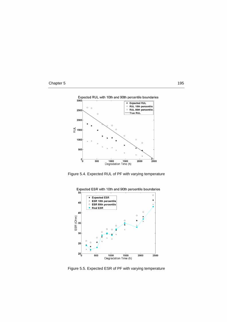
Chapter 5 195

Figure 5.5. Expected ESR of PF with varying temperature

Figure 5.4. Expected RUL of PF with varying temperature

196 Prognostic Algorithms

The goodness of the prediction is assessed through the previously introduced Performance Indexes, which are shown in Table 5.3. Indeed, the obtained PI values are very satisfactory, with good precision and accuracy indexes and a reasonable coverage of the predictions.

Precision Index 0.30

Accuracy Index 0.10

Steadiness Index 0.68

Risk Index 0.50

Coverage Index 0.75

Table 5.3. Performance Indexes of RUL prediction for varying temperature

5.1.5 Conclusions of capacitor prognosis The problem of predicting the RUL for electrolytic capacitors working in

variable operating conditions has been addressed. The data collected during accelerated aging tests have been employed to test the approach. Given the non-stationary operating conditions and, particularly, the varying operational temperature experienced by this kind of components, a new degradation indicator independent from temperature has been proposed. The indicator is defined as the ratio between the ESR measured at temperature TESR and its initial value at the same temperature TESR. Using a physics-based model of the degradation evolution, a Particle Filter-based modeling framework to predict the capacitor RUL have been developed and applied to real degradation data. The effects of the uncertainty of the degradation model associated to the process noise have also been investigated performing a sensitivity analysis on few noise values and evaluating the corresponding performance by means of commonly used prognostic metrics. The performance of the method on real data has been found satisfactory.

Chapter 5 197

5.2 RUL prediction of IGBTs The objective of the present work is to provide a method for predicting

the RUL of IGBTs. The method should also be able to estimate the uncertainty that affects RUL predictions. On Chapter 2 a complete literature review on IGBTs prognosis was provided, however, some of the results are revised here.

The degradation process of IGBTs has been demonstrated to be affected by several sources of uncertainty [32, 33]. Given the characteristics and constraints of the problem, several data-driven or model-based approaches have been suggested with different outcomes. However, RUL prediction has been scarcely addressed provided the difficulties to be faced. This statement is confirmed by the limited number of references with results on real data [29, 31, 32, 35].

A major challenge for the techniques present in the literature is the accurate assessment of IGBTs RUL. Several physical degradation models have been proposed; however, they are not capable of adapting to the different IGBT types and to varying operating conditions. Therefore, IGBT stochasticity is a problem for these predictions. On the other hand, data-driven models are not able to accurately predict the RUL in the long run, mainly because of the minute variation of the failure precursor parameters. Thus, in [29] and [30] a classification of the IGBT health state distributed in three levels (healthy, degraded and failed) was provided, the estimation of the RUL is still a pending issue.

Consequently, in this work, we consider a prognostic method based on both data-driven and physics-based model approaches. Model-based prognostics use an explicit mathematical model of the degradation process to predict the future evolution of the degradation state and, thus, the equipment’s RUL. On the other hand, data-driven prognostics are used when an explicit model of the degradation process is not available, but sufficient data have been collected.

Because of the many factors influencing the performance of prognostic systems, such as (i) the dependence of the algorithm’s accuracy on the quantity of valid reference patterns; (ii) the variability associated to manufacturing conditions and uncertainties in environmental and operating conditions; and (iii)

198 Prognostic Algorithms

the sensory signal relationships with different health states, a single data-driven or physics-based approach would not consider all the available information [29]. Thus, the benefits of gathering both sources of information with specific reference to the problem of predicting the RUL of IGBTs installed in Fully Electric Vehicles (FEVs) have been considered. An ensemble algorithm which leverages the strengths of different sources of information to form a robust unified algorithm for IGBT RUL prediction has been applied.

The three main novelties of the proposed prognostic method are:

• The employment of a bootstrapped aggregation ensemble [47, 48] for directly estimating the RUL of IGBTs together with RUL estimation uncertainty.

• The application and validation of the method with real experimental data from three different IGBT types.

• From the methodology point of view, the input to the prognostic model of a mixture of data-driven and physics-based model information for IGBT monitoring.

The data used to develop the prognostic method and verify its performance are taken from accelerated degradation tests performed on three different types of IGBTs: IR’s IRG4BC30KDpbf punch-through IGBT, FUJI’s FGW15N120VD Trench Field-Stop IGBT and the IXYS IXXN110N65C4H1 Trench XPT GenX4 IGBT, as it was explained on Chapter 4.

The selected variables for IGBT RUL prediction for an online monitoring system are: case temperature (TC), collector current (IC) and collector-emitter voltage (VCE). These variables were selected taking into account the results of accelerated aging tests previously developed and explained in Chapter 4 and confirmed by other researches [35, 36]. The results obtained show that accurately measuring these three variables allows the degradation state of IGBTs to be assessed [29, 35, 36, 37].

Now, the proposed prognostic methodology is explained.

Chapter 5 199

5.2.1 Prognostic method In this section, the implementation of the prognostic method is explained

following these steps:

1. The selection and use of the physics-based model is explained.

2. The employment of data-driven methods to get the degradation patterns is explained.

3. The process of combining the data-driven and physics-based model information into an ensemble method is shown.

Prior to the development of the prognostic method, a brief summary of the available information is done, in which the data collected in the accelerated aging tests is shown.

5.2.1.1 Available information

In order to test and develop the prognostic method, data collected during accelerated aging tests for the three different IGBT types was used. A detailed description of the accelerated aging tests is presented in Chapter 4.

For the sake of simplicity, the results shown in Figure 5.6 were not shown in Chapter 4. The data collected from the accelerated aging tests showed minute variation in the signals before a failure occurred, a characteristic that confirmed the conclusions drawn from the literature review [32, 35, 37, 38]. For a given TC and IC, the VCE value variation with degradation was minute, in the range of 4 to 7 %. This change can be observed in Figure 5.6, where the evolution of the variation of the VCE is shown with respect to the number of degradation cycles for a set TC and IC. Note that the degradation trajectories followed by each of the IGBTs are initially different from one IGBT type to the other. Nevertheless, it can be seen that each IGBT type shows a repeatable trend, which could be learnt by a prognostic algorithm.

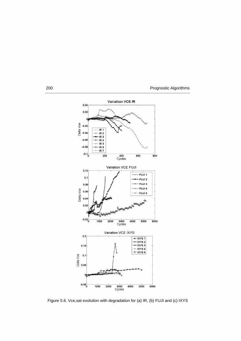
200 Prognostic Algorithms

Figure 5.6. Vce,sat evolution with degradation for (a) IR, (b) FUJI and (c) IXYS

Chapter 5 201

5.2.1.2 Use of the physical model for identifying the

accumulated damage

Now, an analysis of the selected physical model (Eq. 5.26) with respect to the collected data can be made.

The physics-based model selected for our study was developed as part of the LESIT project [39]. It provides the number of cycles to failure at a particular stress level, given by the average (TJ,med) and swing (∆TJ) junction temperature.

Nfi = A∆TJαe( QR∗TJ,med

) (Eq. 5.26)

where, A = 640 and α = -5 are constants, Q = 7.8 ∗ 104 J/mol and R is the gas constant. This model, based on the Arrhenius law, has been adopted since experimental tests suggest that IGBT degradation is mainly caused by thermally activated creeping processes. Furthermore, the model is able to cope with junction temperatures above the nominal temperature of the component such as those encountered in accelerated aging tests.

Bayerer et al. [33] proposed a more refined model based on the LESIT equation for assessing the number of cycles (Nfi) taking into account other parameters that influence the degradation process, such as the power on time or the current per wire. However, their model is not considered in this work since it only applies to IGBTs working with a junction temperature in the range 50 to 150 ºC.

Note that junction average and swing temperature values are employed in the physical model (5.26); however, only the case temperature was available from the measurements. Thus, the junction temperature was estimated from the case temperature, employing Eq. 5.27.

Tj = Tc + Rth ∗ PTOTAL (Eq. 5.27)

Where, Tj is the junction temperature, Tc is the case temperature, Rth is the thermal resistance (provided in component’s datasheet) and PTOTAL represents the total losses, which is the sum of switching and continuous conduction losses [40] that were estimated following the procedure in [41]. It is assumed that an error is being made in Eq. 5.27, as we already know that Rth,

202 Prognostic Algorithms

which this equation considers to be constant, changes slightly with degradation. However, it is expected that he ensemble method is able to cope with this source of noise or inaccuracy.

The junction temperature was then processed by employing the rainflow counting algorithm to obtain the average and swing temperatures during the lifetime for a set time window, as explained in [42]. This algorithm is widely employed for cycles counting in fatigue processes of mechanical devices and electronics [32]. The rainflow counting algorithm was implemented by employing the toolbox developed in [43].

Finally, Miner`s rule [44] was applied to get a value for the accumulated damage from the physics-based model. Miner’s rule assumes linear damage accumulation (Eq. 5.28);

Damage = ∑ NiNfi

ni=1 (Eq. 5.28)

Where, Ni is the number of cycles at a stress level i, and Nfi represents the number of cycles to failure at that particular stress level. It is assumed that the damage is complete when Damage = 1.

The outcome of this process is a prediction of the accumulated damage for each of the IGBTs, which will become an input pattern for the ensemble method.

5.2.1.3 Development of the data-driven degradation patterns

As previously mentioned, the data collected from the accelerated aging tests showed a minute variation in the signals before a failure occurred, confirming the results obtained in [35, 36]. Therefore, the employment of the raw data of the three collected variables together (VCE, IC, and TC), was insufficient to teach to a prognostic algorithm the degradation pattern of IGBTs, as will be later shown in the results section. As a result, the employment of multi-variate analysis was decided to be applied in order to obtain representative degradation patterns to train the hybrid ensemble method. It must be noticed that the aim of these algorithms is not to provide direct RUL predictions, but to generate degradation patterns that will be fed to the ensemble method to produce the RUL predictions.

Chapter 5 203

The selected data-driven models were the following: Self-Organizing Maps (SOM), Artificial Neural Networks (ANN), Mahalanobis Distance (MD) and Principal Component Analysis (PCA). These algorithms were initially selected for several reasons. Firstly, they all are state-of-the-art multi-attribute classification techniques (supervised learning, unsupervised clustering, classification, and statistical inference) which have been widely reported and tested in the literature in different data analysis problems [29, 32, 38]. The aim of such a wide selection is that the different algorithms may perform better than the others on some regions of the data, as stated in [29]. Indeed, the selected ensemble approach has the inherent flexibility to incorporate any desired advanced algorithm, such as Support Vector Machines. Therefore, it is not restricted the employment of any algorithm to obtain the degradation patterns and thus, the above list of selected data-driven models could be extended.

The degradation patterns or indicators, that will be part of the input for the ensemble method, were obtained from the extraction of “residuals” from the application of each of the mentioned data-driven models. “Residuals” are defined as the distance between the output of the data-driven models when trained with healthy operational data of the IGBT, and the actual measured value. This is, the algorithms are trained with raw data values belonging to the healthy state of the IGBT in a certain working conditions. Then, when operational data from degraded conditions is presented to the algorithm, it will still provide an output similar to the one from the healthy state, and thus, a distance can be calculated from the output provided by the algorithm and the actual measured value. The models were trained with data belonging to the initial 10 % of the lifetime operation of the IGBTs, assuming them as healthy state. Then, data measured from more degraded time windows were tested in the models. The distance or “residuals” between the output of the model and the actual measured data were calculated for each algorithm employing the Root Mean Square Error (RMSE). Now, a brief description of the employed data-driven models is provided.

5.2.1.3.1 Self-Organizing Maps (SOM)

SOMs are an unsupervised learning algorithm. SOMs, also known as Kohonen maps, are a neural network model for data clustering [30]. The SOM is

204 Prognostic Algorithms

a two-dimensional projection of a multi-dimensional feature space, which is able to maintain the relevant information about the data. In particular, two vectors that are close in the multidimensional feature space are located in two topologically close SOM units. The SOM uses a neighborhood function to preserve the topological properties of the input space and determine the closest unit distance to the input vector.

In our case, the SOM was trained and tested following the same procedure as in [30] to obtain the degradation patterns.

5.2.1.3.2 Artificial Neural Networks (ANN)

ANN are largely employed for supervised learning purposes, including data fitting or pattern recognition [28, 45]. A back-propagation neural network has been used as a data-driven model. This is a multi-layer NN, including a layer for the input, some hidden-layers and an output layer. The number of hidden layers and the number of neurons vary based on the complexity of the problem. During the training phase, the output values are compared with the correct answers to compute the value of some predefined error-function. The error is then fed back through the network. Using this information, the algorithm adjusts the weights of each connection in order to reduce the value of the error function by some small amount.

In this work, the NN was trained with the healthy data belonging to the Ic and Tc parameters, while the Vce was set as the target value. When new (Ic and Tc) data, belonging to more degraded time windows, was introduced to the algorithm it predicted a Vce value similar to the one observed for the healthy data. As a result, the RMSE value was computed for each of the outcomes from the algorithm and the measured Vce value, obtaining the “residual”.

5.2.1.3.3 Mahalanobis Distance (MD)

MD is a statistical technique employed for data treatment. It differs from the previous learning algorithms in that it is a distance measurement based on the correlations between variables. The MD of an observation x = (x1, x2, … , xN)T from a set of observation with mean µ = (µ1, µ2, … , µN)T and covariance matrix S is defined as:

Chapter 5 205

DM(x) = (x − µ)TS−1(x − µ) (Eq. 5. 29)

For the MD algorithm, the “residuals” where directly obtained through the application of the distance calculation between the healthy state data and data belonging to more degraded time windows.

5.2.1.3.4 Principal Component Analysis (PCA)

Principal Component Analysis is a widely employed method for dimension reduction. PCA is a statistical procedure that uses an orthogonal transformation to convert a set of possibly correlated variables into a set of values of linearly uncorrelated variables called principal components. This transformation is defined in such a way that the first principal component has the largest possible variance. The resulting vectors constitute an uncorrelated orthogonal basis set. The principal components are orthogonal because they are the eigenvectors of the covariance matrix [46].

In our problem, the “residuals” were calculated as follows. The principal component of the healthy state data was initially calculated. Then, the Vce variable belonging to more degraded time windows was projected into that basis. The residuals were calculated through the RMSE calculation between the resulting score of the projection and the actual value of the Vce.

5.2.1.4 Combining data-driven and physics-based models

information into the ensemble method: the

bootstrapped aggregation algorithm

The hybrid approach was considered given two premises. Firstly, data-driven degradation patterns were available, but the patterns were highly stochastic. Secondly, a physics-based model of the degradation was available, but its accuracy was poor (see Case Study below). Therefore, the logical step was to try to mix the different data sources in order to improve the outcome, thus, “hybridizing” the input of the algorithm.

The points previously explained in Sections, 5.2.1.2 and 5.2.1.3, now allow us to explain how to join both physics-based and data-driven models as inputs for the ensemble method.

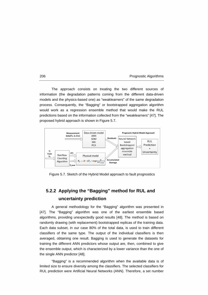
206 Prognostic Algorithms

The approach consists on treating the two different sources of information (the degradation patterns coming from the different data-driven models and the physics-based one) as “weaklearners” of the same degradation process. Consequently, the “Bagging” or bootstrapped aggregation algorithm would work as a regression ensemble method that would make the RUL predictions based on the information collected from the “weaklearners” [47]. The proposed hybrid approach is shown in Figure 5.7.

5.2.2 Applying the “Bagging” method for RUL and uncertainty prediction

A general methodology for the “Bagging” algorithm was presented in [47]. The “Bagging” algorithm was one of the earliest ensemble based algorithms, providing unexpectedly good results [48]. The method is based on randomly drawing (with replacement) bootstrapped replicas of the training data. Each data subset, in our case 80% of the total data, is used to train different classifiers of the same type. The output of the individual classifiers is then averaged, obtaining one result. Bagging is used to generate the datasets for training the different ANN predictors whose output are, then, combined to give the ensemble output, which is characterized by a lower variance than the one of the single ANN predictor [48].

“Bagging” is a recommended algorithm when the available data is of limited size to ensure diversity among the classifiers. The selected classifiers for RUL prediction were Artificial Neural Networks (ANN). Therefore, a set number

Figure 5.7. Sketch of the Hybrid Model approach to fault prognostics

Chapter 5 207

of different ANN was trained with the data belonging to the selected degradation patterns coming from the different IGBTs. The target for those training patterns was the corresponding RUL value for each data point.

5.2.2.1 Uncertainty boundaries assessment

A major issue with the previous algorithm was assessing the uncertainty of the predictions, or in other words, quantifying the confidence on RUL predictions. The possibility of assessing the main sources of uncertainty from bootstrapped ensembles was addressed in Baraldi et al. [28]. Three sources of uncertainty were accounted for when employing a bootstrapped aggregation ensemble. The first is the uncertainty due to model uncertainty (σB), which is studied through the variability in the predictions of the diverse models of the ensemble. Additionally, the uncertainties due to the stochasticity of the degradation process (σA ), and the input noise (σC) of the employed past degradation data were studied. They required that the relationship between the input data and the error of the prognostic model based on its performance on a validation dataset were studied. In this sense, the methodology of approach 2: Bootstrapped ensemble of empirical models trained on sequences of degradation observations and life time data, defined in [28] was followed (see Appendix III).

5.2.2.2 Leave One Out (LOO) Strategy

To analyze the algorithm performance on unseen data, the Leave One Out (LOO) method was employed [30]. This means that a trajectory from an IGBT is not used during the training phase; instead, it is employed only for testing. This is a key point for the algorithm validation. After following the LOO strategy, not only the algorithm performance is being tested, but the algorithm is being validated as well if the accuracy levels are met. It must be highlighted that the testing data has not been shown to the algorithm, and so, the prediction fully relies on the trends “learnt” by the algorithm.

5.2.2.3 Algorithm application pseudo-code

In Table 5.4 the pseudo code for the application of the hybrid ensemble algorithm is summarized.

208 Prognostic Algorithms

Input Raw data (Vce, Ic and Tc) for different IGBT degradation trajectories with the corresponding RUL value for each measurement

Algorithm

Step 1 Obtain the residuals with PCA, MD, ANN and SOM for each degradation trajectory

Step 2 Obtain the predicted damage by the physics-based model for each degradation

trajectory

Step 3 Normalize the data and generate the training matrix with the data from steps 1 and 2,

without the data of one trajectory (LOO procedure). Take a fraction of the training data

for validation

Step 4 Train H neural networks (“bagging ensemble”) with the training matrix and set the

training target as the corresponding RUL values

Step 5 Assess the uncertainty involved in the prediction with the validation dataset following

the procedure set in [28]

Step 6 Test the H neural networks with the trajectory of the component left out in Step 3

Step 7 Calculate the uncertainty boundaries

Output RUL prediction and uncertainty estimation of the left IGBT trajectory

Table 5.4. Pseudo code for the hybrid ensemble application

5.2.3 Case study of IGBTs As mentioned previously, the model was applied to the accelerated

aging tests carried out on different IGBTs, more precisely, 7 IR IGBTs, 5 FUJI IGBTs and 5 IXYS IGBTs were subjected to ageing tests. A detailed description of the aging tests is provided in Chapter 4.

The three selected variables for monitoring were based on the developed experiments and the literature: IC, TC and VCE [29, 32, 35, 49].

With regard to the recorded signals, several problems were observed for prognosis. The variation of the signals with degradation can be considered small, on the order of hundredths of mV, which is in line with other reports [35]. This is especially true for the VCE, whose variation for a given value of IC and TC is directly related to the degradation state. Secondly, the evolution of the Vce with the degradation of the IGBT shows an abrupt change at the end-of-life

Chapter 5 209

(EOL) of the component. However, with longer operation times within the safe operation area (SOA) of the component, more consistent and regular patterns are expected, thus showing better prognosticability.

In order to deal with the previously mentioned problems, it was decided to employ the residuals from the data-driven models, which allowed clear degradation patterns to be obtained.

After the degradation tests, the three recorded signals (TC, IC, VCE) containing the degradation patterns of the tested IGBTs were available. The cycles endured by each IGBT are recalled in Table 5.5.

In Figure. 5.8 the number of cycles that an IGBT would endure

depending on junction temperature swing is presented for different physical models. The line made up of squares represents the lifetime estimation provided by the LESIT equation (Eq. 5.26) for an average junction temperature of 125 ºC and different junction temperature deltas. The line made up of circles represents the lifetime estimation made by Bayerer et al. [33] for an average junction temperature of 125ºC. The line made up of diamonds represents the estimation of the LESIT equation for an average junction temperature of 230 ºC, which is the average junction temperature of the degraded components. Finally, the rest of the data points represent the failures of the different IGBTs tested. It can be seen that the physical model from Eq. 5.26 is able to approximately estimate the RUL of the components at least in the order of magnitude.

IGBT

Type 1 2 3 4 5 6 7

IR 710 704 500 400 300 400 328

FUJI 1524 2100 2150 2803 5200 - -

IXYS 5007 3186 2742 3200 3000 - -

Table 5.5. Number of thermal cycles endured

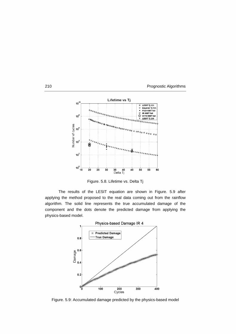
210 Prognostic Algorithms

Figure. 5.8. Lifetime vs. Delta Tj

The results of the LESIT equation are shown in Figure. 5.9 after applying the method proposed to the real data coming out from the rainflow algorithm. The solid line represents the true accumulated damage of the component and the dots denote the predicted damage from applying the physics-based model.

Figure. 5.9: Accumulated damage predicted by the physics-based model

Chapter 5 211

It can be seen that the prediction for the physics-based model is not accurate enough, underestimating the damage caused to the component. However, it can be observed that it is able to estimate it within the same order of magnitude. This means that the model is able to replicate at a certain level the behavior of the ongoing degradation mechanism represented.

The computation of the aforementioned data-driven algorithms allowed us to detect when the behavior of the signals was different from the one presented for the training and corresponding to the healthy state. The application of the multi-variate analysis discovered clear degradation patterns. Figure. 5.10 shows the residuals obtained for the lifetime of IR 4 IGBT for the different data-driven models.

Figure. 5.10. Data-driven algorithm residuals for IR 4

Figure. 5.10 shows that an abrupt change of the residuals was detected close to the end-of-life of the component, which indicates it is close to fail. However, such an abrupt change is a known problem for data-driven prognostics, as the signals are flat during most of the component life, thus showing a lack of relevant information for long periods of time. This problem is addressed here, through the mixture of both data-driven and physics based models.

212 Prognostic Algorithms

After collecting the different “weaklearners” (e.g. the results of the data-driven and physics based models application), the matrix for training the ensemble method was built. Columns contained the data for each “weaklearner”, e.g. the results from the application of the data-driven and physics-based models. Rows represented the values corresponding to a time window. The target of the algorithm was a column containing the associated RUL for each time window of the degradation process. Finally, the algorithm was trained and tested employing the LOO strategy.

In order to study the performance of the predictions made by the hybrid ensemble model, the following performance indexes (PI) were selected: precision and accuracy, which are defined in Chapter 5.1.3.2. and in [49]. Attending to the equations of the indexes, the lower the value, the better the prediction is. A final index was also studied in order to compare the results of the prognostic algorithm with respect to the one from other researches [34]. This is the Relative Accuracy (RA), defined as:

RA = 100 ∗ (1 − RUL∗−RUL′RUL∗

) (Eq. 5.30)

Where, RUL* is the True RUL and RUL’ is the predicted RUL. The True RUL stands for the RUL obtained experimentally. The closer the RA value to 100, the better the predictions are.

5.2.4 Results of prognostic algorithms The prognostic method described was applied to the accelerated aging

tests data. The method was separately applied to the data of 7 IR, 5 FUJI and 5 IXYS IGBTs. The LOO methodology was employed during the whole testing process. The figures show the following parameters. The True RUL is the experimentally measured RUL, which is a decreasing straight line beginning at the total lifetime of the IGBT and finishing at the end-of-life of the component at 0 remaining cycles. The Predicted RUL is the outcome of the algorithm, together with the lower and upper uncertainty boundaries.

In order to test and validate the hybrid-ensemble methodology, initially, different tests were carried out on IR IGBTs dataset. The results can be seen in Figure. 5.11, where the data of 6 IGBT degradation trajectories were employed for training and the data from IR 4 was employed for testing.

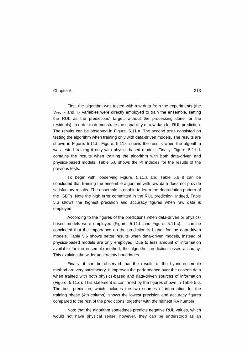
Chapter 5 213

First, the algorithm was tested with raw data from the experiments (the VCE, IC and TC variables were directly employed to train the ensemble, setting the RUL as the predictions’ target, without the processing done for the residuals), in order to demonstrate the capability of raw data for RUL prediction. The results can be observed in Figure. 5.11.a. The second tests consisted on testing the algorithm when training only with data-driven models. The results are shown in Figure. 5.11.b. Figure. 5.11.c shows the results when the algorithm was tested training it only with physics-based models. Finally, Figure. 5.11.d. contains the results when training the algorithm with both data-driven and physics-based models. Table 5.6 shows the PI indexes for the results of the previous tests.

To begin with, observing Figure. 5.11.a and Table 5.6 it can be concluded that training the ensemble algorithm with raw data does not provide satisfactory results. The ensemble is unable to learn the degradation pattern of the IGBTs. Note the high error committed in the RUL prediction. Indeed, Table 5.6 shows the highest precision and accuracy figures when raw data is employed.

According to the figures of the predictions when data-driven or physics-based models were employed (Figure. 5.11.b and Figure. 5.11.c), it can be concluded that the importance on the prediction is higher for the data-driven models. Table 5.6 shows better results when data-driven models, instead of physics-based models are only employed. Due to less amount of information available for the ensemble method, the algorithm prediction losses accuracy. This explains the wider uncertainty boundaries.

Finally, it can be observed that the results of the hybrid-ensemble method are very satisfactory. It improves the performance over the unseen data when trained with both physics-based and data-driven sources of information (Figure. 5.11.d). This statement is confirmed by the figures shown in Table 5.6. The best prediction, which includes the two sources of information for the training phase (4th column), shows the lowest precision and accuracy figures compared to the rest of the predictions, together with the highest RA number.

Note that the algorithm sometimes predicts negative RUL values, which would not have physical sense; however, they can be understood as an

214 Prognostic Algorithms

overestimation of the damage generated to the component under test, and thus, a prediction that the component lifetime should already be over.

A final validation test was done in order to state which of the data-driven models provide more information about the degradation of the IGBTs. Therefore, tests were run with both physics-based and data-driven models, but leaving out one of the data-driven models each time. Results are shown in Table 5.7. The worst results were obtained when the degradation trajectories extracted by the ANN algorithm were left out. Thus, ANN is the best data-driven algorithm for collecting information about IGBTs degradation trajectories. In this sense, MD would be the worst algorithm.

Following the results observed in this section, it can be concluded that the hybrid approach, thus, mixing the data-driven and physics-based models with the ensemble method, provides the best results.

Prediction without ANN

Prediction without PCA

Prediction without MD

Prediction without SOM

Precision 6.1539 4.4752 3.8526 5.2420

Accuracy 2.9711 2.2082 1.9832 2.0965

RA 62.6698 71.3462 74.44 66.0415

Table 5.7. Average values of the PI for RUL prediction for IR 4

Prediction with raw data IR 4

Prediction with data-driven models

Prediction with physics-based model

Prediction with all sources of information

Precision 5.0661 2.4731 3.1758 1.1216

Accuracy 1.6161 0.8385 0.9174 0.3479

RA 60.0661 82.1370 80.2555 92.3064

Table 5.6. Average values of the PI for RUL predictions for IR4

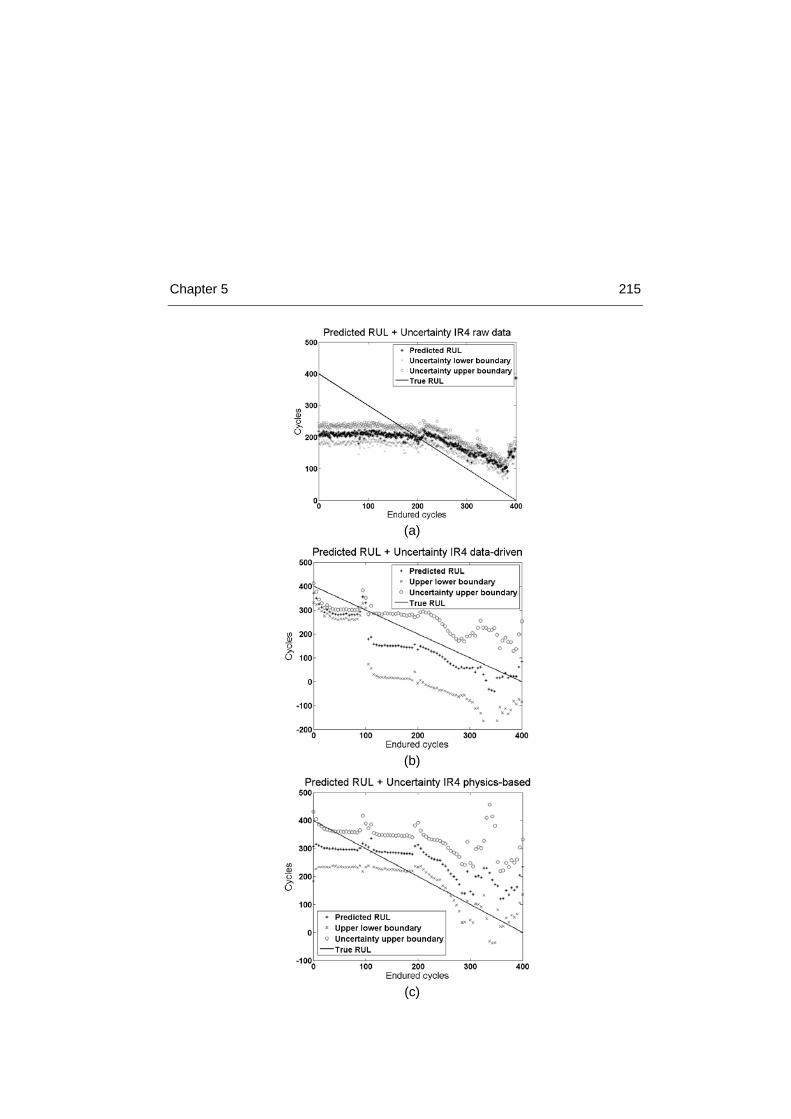
Chapter 5 215

(a)

(b)

(c)

216 Prognostic Algorithms

(d)

Figure. 5.11. RUL predictions for IR 4 only employing (a) raw data, (b) data-

driven models, (c) physics-based model, (d) data-driven and physics-based

Following the previous results, it was decided to do the ongoing tests including both physics-based and all the data-driven models to test the ensemble on the remaining IGBT models. Table 5.8 and Figure. 5.12 gather the results of the final tests made with the algorithm regarding the rest of IGBTs.

Figure. 5.12.a shows the results when the algorithm is trained only with IR IGBTs and testing it on IR6. Figure. 5.12.b shows the results when the algorithm is trained only with FUJI IGBTs and testing it on FUJI 4. Figure. 5.12.c shows the results when the algorithm is trained only with FUJI IGBTs and testing it on IXYS 4.

Despite the good values obtained in Table 5.8, some conclusions can be extracted. Firstly, the predictions made to IR IGBTs are better than the ones for the other IGBT types. This might be explained due to the bigger number of available trajectories for the training phase on IR IGBTs. Following the LOO strategy, there are only 4 IGBT trajectories available for FUJI and IXYS IGBTs during the ensemble method training. Nevertheless, the obtained accuracy and RA values are acceptable.

Finally, taking into account that the algorithm seemed to improve with more available data, we decided to include within the training matrix all the degradation patterns, independently from the IGBT type. In order to test this, the degradation patterns of all the available IGBTs, that is, the 16 degradation

Chapter 5 217

trajectories from IR, FUJI and IXYS IGBTs, were included within the training algorithm, except for the IGBT being tested, IGBT IR 6 indeed. The results are shown on the 4th column of Table 5.8 and Figure. 5.12.d. It can be concluded that overall the precision and accuracy were not improved with respect to the training of data coming solely from the IGBTs of its type. This is the consequence of the differences between the trends followed by each IGBT type. However, it has been observed that a greater number of degradation patterns from the same IGBT type improve the performance of the ensemble.

Given the scarce quantity of references regarding IGBT RUL predictions, it is difficult to compare the obtained results with other researches. However, in order to assess the goodness of the RUL predictions with the proposed ensemble method, precision values close to 1 and accuracy values around 0.3 were suggested in [49]. With respect to RA parameter, which employment is introduced in [34] for MOSFET RUL prediction assessment, values between 60 and 90 are found in good predictions. Therefore, we can confirm that the obtained values for the PI and the results of the predictions, overall, are very satisfactory.

PREDICTIONS IR 6

PREDICTIONS FUJI 4

PREDICTION IXYS 4

PREDICTIONS IR 6 MIX IGBT DATA

Precision 1.0055 3.4904 3.6226 1.9165

Accuracy 0.2143 0.5139 0.8938 0.5578

RA 92.7160 93.1602 86.2144 82.9975

Table 5.8. Average values of the PI for RUL prediction of IR 6, FUJI 4, IXYS 4

and IR 6 with mixed data

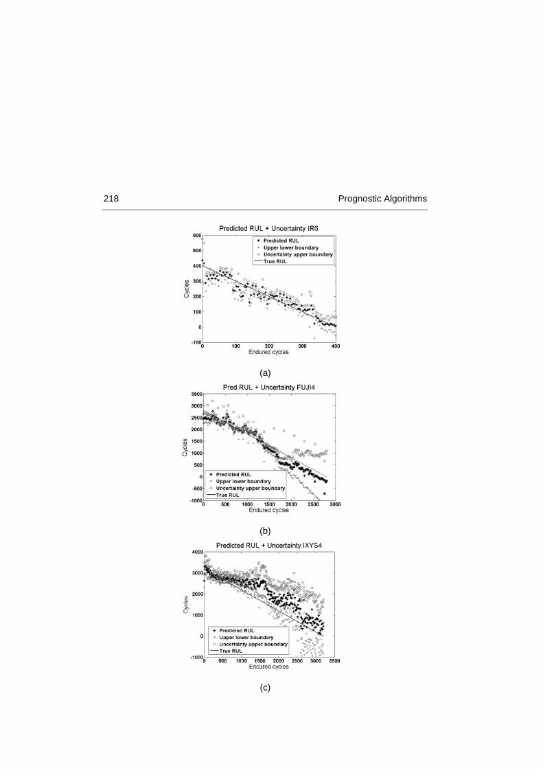
218 Prognostic Algorithms

(a)

(b)

(c)

Chapter 5 219

(d)

Figure. 5.12. RUL predictions for (a) IR 6, (b) FUJI 4, (c) IXYS 5 and (d) IR 6

with Mixed data

5.2.5 Conclusions of IGBT prognosis In this research, the problem of predicting the RUL of IGBTs has been

addressed. Although IGBT lifetime models have been previously suggested, IGBT RUL prediction is still a major issue given the stochasticity of their degradation process. In this work, a hybrid ensemble algorithm was presented and tested. Other researches [34, 50] rely on experimentally obtained degradation models and Particle Filter (PF) approaches to predict the RUL of semiconductors. The advantage of the proposed method is that small amounts of data are required. However, its performance decreases with components that do not follow the set trend.

The advantages of the algorithm proposed in this work are that it is able to “adapt” to the singularities of each IGBT type, providing accurate RUL predictions and the uncertainty boundaries related to them. However, it requires a bigger amount of data to be trained.

The goodness of the selected methodology can be concluded after analyzing the results. The hybrid ensemble has demonstrated its validity in predicting the RUL of IGBTs with information provided by physics-based and data-driven models. Moreover, the algorithm improves its performance when

220 Prognostic Algorithms

more information and degradation patterns become available. Therefore, the algorithm is able to “learn” the degradation behavior for each IGBT type. The algorithm has been successfully validated through the development of different tests, and its validity for IGBT RUL prediction has been proved. Thanks to the hybridization of the data sources, the performance of the algorithm is boosted.

To sum up, a hybrid ensemble based on the “Bagging” method for direct RUL prediction of IGBTs has been proposed. This model mixes the information coming from physics-based and data-driven models. The problem of assessing the uncertainty associated with RUL prediction has also been addressed. The performance of the method was analyzed using performance metrics. The hybrid model was tested on experimental data from accelerated aging tests of IGBTs. The satisfactory results support the employment of the method on a PHM system.

5.3 Conclusion of prognostic algorithms In this Chapter, the results of the accelerated aging tests were

employed to develop the prognostic algorithms for RUL estimation. The data of accelerated aging tests was employed for training of the algorithm in the case of IGBTs, and for validation of the algorithms in both cases for capacitors and IGBTs.

The obtained results were satisfactory, fulfilling the statements required for the PHM system stated in Chapter 1 and the work claimed to be beyond the state-of-the-art in Chapter 2. The predictions have been provided with uncertainty boundaries and the algorithms are able to take into account the varying operating conditions.

A still pending issue would be the testing of the suggested hardware and prognostic algorithms on a real FEV on-board application. This would imply porting the algorithms into a portable device with its limitations of memory and data processing. However, these topics are left out of the present work, due to the lack of a testing platform for the final system, although the final implementation of the algorithms should take into account these facts.

Chapter 5 221

5.4 References [1] E. Zio, “Prognostics and health management of industrial equipment,”

Diagnostics and Prognostics of Engineering Systems: Methods and Techniques, 2012

[2] A. Doucet, “On sequential Monte Carlo methods for Bayesian filtering,” Dept. Eng., Univ. Cambridge, UK, Technical Report, 1998

[3] K. Abdennadher, P. Venet, G. Rojat, J.M. Rétif, C. Rosset, “A real-time predictive-maintenance system of aluminum electrolytic capacitors used in uninterrupted power supplies,” IEEE Transactions on Industry Applications, vol. 46 ,pp. 1644-1652, 2010

[4] M.S. Arulampalam, S. Maskell, N. Gordon, T. Clapp, “A tutorial on particle filters for online nonlinear/non-Gaussian Bayesian tracking,” IEEE Transactions on Signal Processing, vol. 50, pp. 174-188, 2002

[5] Y. Hu, P. Baraldi, F. Di Maio, and E. Zio, “A particle filtering and kernel smoothing-based approach for new design component prognostics,” Reliability Engineering & System Safety, 2014

[6] B.D. Anderson, J.B. Moore, “Optimal filtering,” Englewood Cliffs (NJ), Prentice Hall, 1979

[7] A. Doucet, J.F.G. De Freitas, N.J. Gordon, “Sequential Monte Carlo methods in practice,” New York: Springer-Verlag, 2001

[8] P. Lall, R. Lowe, K. Goebel, “Extended kalman filter models and resistance spectroscopy for prognostication and health monitoring of lead free electronics under vibration,” in Reliability, IEEE Transactions on, vol. 61, pp. 858-871, 2012

[9] A. Doucet, N.J. Gordon, and V. Krishnamurthy, “Particle filters for state estimation of jump Markov linear systems,” in Signal Processing, IEEE Transactions on, vol. 49, pp. 613-624, 2001

[10] W. He, N. Williard, M. Osterman, M. Pecht, “Prognostics of lithium-ion batteries based on Dempster-Shafer theory and the Bayesian Monte Carlo method,” Journal of Power Sources, vol. 196, pp. 10314-10321, 2011

[11] F. Gustafsson, “Particle filter theory and practice with positioning applications,” IEEE Aerospace and Electronic Systems Magazine, vol. 25,, pp. 53-81, 2010

222 Prognostic Algorithms

[12] F. Cadini, E. Zio, D. Avram, “Monte Carlo-based filtering for fatigue crack growth estimation,” in Probabilistic Engineering Mechanics, vol. 24, pp. 367-373, 2009

[13] A. Doucet, S. Godsill, C. Andrieu, “On sequential Monte Carlo sampling methods for Bayesian filtering,” Statistical Computing, vol. 10, pp. 197-208, 2011

[14] M. Orchard, F. Tobar, G. Vachtsevanos; “Outer feedback correction loops in particle filtering-based prognostic algorithms,” Statistical performance comparison. Stud Inform Control, vol. 18, pp. 295-304, 2009

[15] S. Saha, K. Goebel, S. Poll, J. Christophersen; “Prognostics methods for battery health monitoring using a Bayesian framework,” Instrumentation and Measurement, IEEE Transactions on, vol. 58, pp. 291-296., 2009

[16] P. Baraldi, F. Cadini, F. Mangili, and E. Zio, “Model-based and data-driven prognostics under different available information,” Probabilistic Engineering Mechanics, vol. 32, pp. 66-79, 2013

[17] E. Zio, G. Peloni, “Particle filtering prognostic estimation of the remaining useful life of nonlinear components,” Reliability Engineering & System Safety, vol. 96, 2011

[18] D. An, J.H. Choi, N.H. Kim, “Prognostics 101: A tutorial for particle filter-based prognostics algorithm using Matlab,” in Reliability Engineering and System Safety, vol. 115, pp. 161-169, 2013

[19] M.L. Gasperi, “Life prediction model for aluminum electrolytic capacitors,” Conference Record - IAS Annual Meeting , IEEE Industry Applications Society, vol. 3, pp. 1347-1351, 1996

[20] M. Hao, and L. Wang, “Fault diagnosis and failure prediction of aluminum electrolytic capacitors in power electronic converters,” Industrial Electronics Society, IECON 2005, 31st Annual Conference of IEEE, pp. 6, 2005

[21] P. Baraldi, F. Cadini, F. Mangili, E. Zio; “Model-based and data-driven prognostics under different available information,” Probabilistic Engineering Mechanics, Elsevier, vol. 32, pp.66-79, 2013

[22] P. Venet, H. Darnand, and G. Grellet, “Detection of faults of filter capacitors in a converter. Application to predictive maintenance,” in Proceedings. International Telecommunication Energy Conference, pp. 229–234, 1993

Chapter 5 223

[23] A.C. Cameron, F.A.G. Windmeijer, “An R-squared measure of goodness of fit for some common nonlinear regression models,” Journal of Econometrics, vol. 77, pp. 329-342, 1997

[24] F. Di Maio, K.L. Tsui, E. Zio, “Combining Relevance Vector Machines and exponential regression for bearing residual life estimation,” Mechanical Systems and Signal Processing, 31, pp. 405-427, 2012

[25] KEMET Electronics Corporation, Technical Notes (2014). Screw Terminal Aluminum Electrolytic Capacitors ALS30/31 Series, pp. 1-14

[26] M.E. Orchard, G.J. Vachtsevanos, “A particle-filtering approach for on-line fault diagnosis and failure prognosis,” Transactions of the Institute of Measurement and Control, vol. 31, pp. 221-246., 2009

[27] B.E. Olivares, C. Munoz, M.E. Orchard, J.F. Silva, “Particle-filtering-based prognosis framework for energy storage devices with a statistical characterization of state-of-health regeneration phenomena,” in Instrumentation and Measurement, IEEE Transactions on, vol. 62, 2013

[28] P. Baraldi, F. Mangili, E. Zio, “Investigation of uncertainty treatment capability of model-based and data-driven prognostic methods using simulated data,” Reliability Engineering & System Safety, vol. 112, pp. 94-108, 2013

[29] P. Tamilselvan, P. Wang, M. Pecht; "A multi-attribute classification fusion system for insulated gate bipolar transistor diagnostics," Microelectronics Reliability, vol. 53, no. 8, pp. 1117-1129, 2013

[30] M. Rigamonti, P. Baraldi, E. Zio, A. Alessi, D. Astigarraga, A. Galarza; "A Self-Organizing Map-Based Monitoring System for Insulated Gate Bipolar Transistors Operating in Fully Electric Vehicle," Annual Conference of the Prognostic and Health Management Society 2015, vol. 6., 2015

[31] A. Hensler, J. Lutz, M. Thoben, K. Guth; "First power cycling results of improved packaging technologies for hybrid electrical vehicle applications," Integrated Power Electronics Systems (CIPS), 2010 6th International Conference on, IEEE, 2010

[32] S. Yang, D. Xiang, A. Bryant, P. Mawby, L. Ran, P. Tavner,; "Condition monitoring for device reliability in power electronic converters: a review," Power Electronics, IEEE Transactions on, vol. 25, no. 11, pp. 2734-2752, 2010

224 Prognostic Algorithms

[33] R. Bayerer, T. Herrmann, T. Licht, J. Lutz, M. Feller; "Model for Power Cycling lifetime of IGBT Modules: various factors influencing lifetime," Integrated Power Systems (CIPS), 2008 5th International Conference on VDE, pp. 1, 2008

[34] J. Celaya, A. Saxena, S. Kulkarni, S. Saha, K. Goebel; “Prognostics approach for power MOSFET under thermal-stress aging,” in Reliability and Maintainability Symposium (RAMS), 2012 Proceedings Annual, pp. 1-6, 2012

[35] V. Smet, F. Forest, J. Huselstein, F. Richardeau, Z. Khatir, S. Lefebvre, M. Berkani; "Ageing and Failure Modes of IGBT Modules in High-Temperature Power Cycling," Industrial Electronics, IEEE Transactions on, vol. 58, no. 10, pp. 4931-4941, 2011

[36] N. Patil, J. Celaya, D. Das, K. Goebel, M. Pecht; "Precursor Parameter Identification for Insulated Gate Bipolar Transistor (IGBT) Prognostics," in Reliability, IEEE Transactions on , vol.58, no.2, pp.271-276, June 2009

[37] Y. Xiong; X. Cheng; Z. Shen; C. Mi, H. Wu; V. Garg;, “A prognostic and warning system for power electronic modules in electric, hybrid, and fuel cell vehicles,” Industrial Electronics, IEEE Transactions on, vol. 55, no. 6, pp. 2268–2276, Oct. 2008

[38] H. Oh, B. Han, P. McCluskey, C. Han, B.D. Youn; "Physics-of-Failure, Condition Monitoring and Prognostics of Insulated Gate Bipolar Transistor Modules: A Review," Power Electronics, IEEE Transactions on, 30(5), 2413-2426, 2015

[39] M. Held, P. Jacob, G. Nicoletti, P. Scacco, M.H. Poech,; "Fast power cycling test of IGBT modules in traction application," in Power Electronics and Drive Systems, 1997. Proceedings, 1997 International Conference on , vol.1, no., pp.425-430 vol.1, 26-29, May 1997

[40] H. Huang and P.A. Mawby;, "A Lifetime Estimation Technique for Voltage Source Inverters," in Power Electronics, IEEE Transactions on, vol.28, no.8, pp.4113-4119, Aug. 2013

[41] SEMIKRON International GmbH, 2011, “Application Manual Power Semiconductors”, ISLE, ISBN: 978-3-938843-66-6, 2011

[42] M. Ciappa; F. Carbognani; P. Cova; W. Fichtner; “A novel thermomechanics-based lifetime prediction model for cycle fatigue,” Microelectronics Reliability, vol. 42, no. 9–11, pp. 1653–1658, 2002

Chapter 5 225

[43] A. Nieslony, “Determination of fragments of multiaxial service loading strongly influencing the fatigue of machine components,” Mechanical Systems and Signal Processing, Vol. 23, pp. 2712-2721, 2009

[44] M. Miner; “Cumulative damage in fatigue,” Transactions of the American Society of Mechanical Engineering, 67, pp. A159–A164, 1945

[45] K. Goebel; B. Saha; A. Saxena; “A Comparison of Three Data-Driven Algorithms for Prognostics,” in 62nd meeting of the society for machinery failure prevention technology (MFPT) , pp. 119-131, 2008

[46] H. Abdi, and L.J. Williams, "Principal component analysis," Wiley Interdisciplinary Reviews: Computational Statistics, vol. 2, pp. 433–459, 2010

[47] R. Polikar, "Ensemble based systems in decision making," in Circuits and Systems Magazine, IEEE, vol.6, no.3, pp.21-45, 2006

[48] L. Breiman; “Bagging predictors,” Machine Learning, vol. 24, no. 2, pp. 123-140, 1996

[49] M. Rigamonti, P. Baraldi, E. Zio, D. Astigarraga, A. Galarza; "Particle Filter-Based Prognostics for an Electrolytic Capacitor Working in Variable Operating Conditions," in Power Electronics, IEEE Transactions on , vol.31, no.2, pp.1567-1575, Feb. 2016

[50] N. Patil, D. Das, M. Pecht; “A prognostic approach for non-punch through and field stop IGBTs,” in Microelectronics Reliability, vol. 52, no 3, p. 482-488, 2012

[51] B. Alvsten, “Electrolytic capacitors theory and application,” RIFA Electrolytic Capacitors, Sweden, 1995

Chapter 6

6 Research Findings and

Future Work

In this chapter, the main research findings will be collected and summarized. The contributions made to the state-of-art will be compiled as well.

6.1 Findings of the investigation Initially, the background on different PHM systems development was

reviewed. It was stated that no examples on the automotive industry are publicly available, although examples referring to military and aerospace applications were found. The foundation of the PHM Society in 2009 showed the increasing interest that is arising around monitoring systems.

Then, the state-of-the-art for reliability analysis of components and the evolution towards prognostics was presented. A general description and the advantages of prognostic methodologies were explained.

A final introduction to the methodology that has been followed was done. All the previous information, allowed us moving to the chapters containing the information on the implementation of the PHM methodology on the FEV powertrain.

228 Research Findings & Future Work

The findings of the developed investigation are summarized for each chapter.

6.1.1 Regarding the State-of-the-art • Real cases of PHMS implementation were analyzed. PHMS were

found out to be at an infant stage. The few real applications observed are focused on safety critical industries, such as aerospace and military. The main reason is the initial high costs associated to its development with respect to research on sensory and data acquisition systems and advanced algorithms. No real applications were found on the automotive industry, although an increasing amount of patents in the recent years point to a great interest to PHMS implementation in the near future.

• Power Electronic systems reliability was analyzed. Power electronic systems are a good candidate to employ PHMS, given the failure rate of some of the components. Despite the lack of public data, this perception has extended to FEV consumers, which are concerned about their reliability and safety. Following the reports of industry based surveys and HEMIS project results, the electrolytic capacitor and semiconductor devices were selected to be further studied.

• In order to study the reliability and the degradation process of components, accelerated aging tests are a common practice in the industry. Different aging stressors are proposed (thermal, electrical, mechanical, etc.) depending on the component application. Accelerated aging tests are suggested for failure mechanism and failure precursor parameter identification, as well as, operating data collection. Data collected from accelerated aging tests is employed for algorithm development.

• A pending ability to be reviewed of PHMS is Prognosis. Prognosis is the ability of assessing the health state of components and predicting its RUL. Different prognostic approaches including physics-based, data-driven and hybrid were exposed. The selection of the approach depends on the data and information available. Different

Chapter 6 229

methodologies were suggested in literature for electrolytic capacitor and IGBT prognosis. However, some improvements to the suggested methodologies were observed.

6.1.2 Regarding the Failure Modes and Failure Precursor Parameters on electrolytic capacitors and IGBTs

The physical structure of components was reviewed. Then, the most reported failure mode and mechanisms were analyzed for both electrolytic capacitors and IGBTs.

• Electrolytic capacitors mainly degrade because of thermal-stresses, producing the dry-out of the wet electrolyte. This produces an increase of the ESR and a decrease of the capacity, thus, increasing overall losses, and finally, system malfunction.

• IGBTs degrade due to thermally activated induced fatigue stresses, worsening with higher junction temperature variations. IGBT failure mechanisms range from increased losses, to short-circuit or open circuit. The main failure mechanisms are package related failures, bond-wire lift-off and die-attach degradation.

The conclusions for the analyzed failure precursor parameters were:

• Capacity and ESR were selected to be monitored for electrolytic capacitor degradation assessment. In order to capture the environmental stressors, the surface temperature was also suggested.

• TC, IC, VCE, VG and IG variables were selected to be monitored for IGBT degradation assessment. Nevertheless, several researches claim that a small variation of the signal was observed and accurate measurement was required.

230 Research Findings & Future Work

6.1.3 Regarding the Accelerated Aging Tests • The hardware architecture to collect data for both laboratory

experiments and FEV onboard monitoring were exposed. The accuracy of the measurement systems was also studied. The selected sensors were proved to properly assess the degradation of components. The designed hardware for onboard monitoring was successfully tested on laboratory environment.

• Thermal accelerated aging tests were performed on electrolytic capacitors from KEMET. The tests proved the results reviewed, an increase of the ESR and a decrease of the capacitance were observed. Useful degradation data and patterns were collected for algorithm development.

• Electrothermal accelerated aging tests were performed on IGBTs. The tests proved a variation due to the degradation of the VCE signal for a given IC and TC values for the three different IGBT types. The measurement of the discrete variables VCE,SAT and VGE,TH was proved to provide useful information as well. However, owing to the different measurement process they were not suggested for a final system. In short, an accurate measurement of the three parameters (TC, IC, VCE) was identified to allow assessing the health state of IGBTs.

• The failure mechanisms of IGBTs were analyzed through destructive testing. The results of the degradation were observed with a LEICA optic microscope. The images show different consequences depending on the IGBT type. Die-attach degradation and cracks on the die were observed. The large junction temperatures produced severe damages on the components. Thus, it is assumed that in a nominal range of variation, different degradation mechanisms could also be induced, such as bond wire lift-off, which was not observed in this investigation. Consequently, the most relevant failure modes observed are package-related failures due to mechanical fatigue stresses.

Chapter 6 231

6.1.4 Regarding the Prognostic Algorithms Once the degradation data of the accelerated aging tests became

available, the development of the prognostic algorithms was addressed.

• A Particle-Filtering algorithm (PF) was selected for RUL prediction of capacitors. The tests performed on the collected data from accelerated aging tests showed that the model is able to accurately predict the RUL. Consequently, the algorithm is valid for implementation on a PHMS.

• A hybrid-ensemble of physics-based and data-driven algorithms was implemented for IGBT RUL prediction. The ensemble of different data sources enriched the model and boosted its performance. The training and validation phase done with accelerated aging tests data and following the LOO strategy, suggest that the algorithm is able to accurately predict the RUL of components when fed with enough data.

Hence, the final outcome of this research work shows that the followed methodology for PHM implementation allows predicting the RUL of components onboard a FEV. The steps of the followed methodology are:

o Identification of the main failure modes and mechanisms.

o Identification of the failure precursor parameters.

o Development of onboard systems for failure precursor parameter monitoring.

o Development of accelerated aging tests for experimental data collection.

o Development of the prognostic algorithms.

o Testing of the algorithms on the collected experimental data.

6.2 Future Work In this work the implementation of a PHM methodology for RUL

prediction of most critical components of FEV powertrain is addressed.

232 Research Findings & Future Work

However, certain aspects of the research are still pending and could be further investigated in future research works.

• A first major issue arises with respect to cost analysis. PHM systems have been implemented within safety critical applications, where costs are a secondary factor when introducing safety improving components. A detailed costs analysis should be carried out for PHM system design. The costs analysis should take into account the costs associated to accelerated aging tests, as well as the equipment and the expert knowledge required for prognostic software development. Finally, the advantages and cost savings due to the PHM implementation should be also analyzed. Cost saving related to the ability of maintenance planning and abrupt stoppage avoidance should be studied. Indeed, a detailed costs analysis would help to take management decisions.

• The implementation of PHM systems in the future should point towards Prognostic and Health Management systems. Fault management, including detection, diagnosis and prognosis should be included as a whole. As well as the analysis of the entire lifecycle of the component from its design phase to disposal.

• A pending issue regarding PHM implementation is the porting of the algorithms into portable computer devices for onboard analysis. The increased complexity of the prognostic algorithms developed in powerful PCs, makes it difficult to implement the algorithms into state-of-the-art portable microcontrollers such as the ones employed in automotive applications. In the HEMIS project, the PF algorithm was partially tested within a Linux based low cost portable computer (Beagle Board). However, the porting of the ensemble algorithm for IGBT was unsuccessful. Further research on algorithms porting should be done.

• Testing of the suggested sensory systems and algorithms should be done on a real FEV in order to fully validate the PHMS and analyze its industrialization possibility.

7 I. Appendix A:

Introduction to Reliability

Engineering

7.1 Reliability Engineering Reliability engineering covers a wide range of topics concerning items

lifetime. Due to historical misleading definitions, lack of proper documentation and difficulties on formulation, disparate views of the problem have been given.

The modern meaning of reliability comes from the World War II. The U.S. military meant by reliability “that a product would operate when expected”, which is nowadays more related to “mission readiness”. During the WWII big issues arose from the inherent unreliability of electronics and fatigue issues, due to the new manufacturing processes. As a result, major effort was put by the Department of Defense (DoD) into improving the reliability and the quality of the products in the whole manufacturing process and supply chain. Later, that philosophy was exported by J. R. Juran and W. E. Deming to Japan and created the so-called “Japanese quality revolution”, applying the principles of “total quality management”. In 1952, the Advisory Group on Reliability of Electronic Equipment (AGREE) was set in the US. AGREE concluded that in order to break with the high ownership costs due to low reliability, disciplines must be laid down as integral activities in the development cycle. This mainly

234 Reliability Engineering

implied increasing the component testing hours prior to selling. The AGREE report was set as the US Military Standard (MIL-STD 781). [3]

In [1] a common definition of reliability is provided: “Reliability is the ability of an item to perform a required function under stated conditions for a stated period of time”.

It can be derived from the definition that reliability is closely related to the probability that an item (it can be a system, product, subsystem, assembly, component, part, etc [2]) will perform its intended function for a specified interval under stated conditions. In classical reliability, a single product, unit, or component is generally considered to have two states, operational and failed. In classic reliability, R(t), is the probability that the product is in the operational state up to time t. At time 0, the product is assumed to be good, and the product must eventually fail, so R(0) = 1, R(∞) = 0, and R(t) is a non-increasing function. If there is a mission with duration T, the classic reliability for that mission is R(T). It can be expressed mathematically as:

𝑅(𝑡) = Pr𝑇 > 𝑡 = ∫ 𝑓(𝑥)𝑑𝑥∞𝑡 (Eq. 1)

Where, f(x) is the failure probability density function (pdf) and t is the length of the time period. Upon the previous probability model, a reliability theory was built, which meant that measures (metrics) for reliability could be obtained. In [4], several common metrics employed for reliability are presented. These are the failure rate, the mean time to failure (MTTF), the mean time to repair (MTTR) and the availability.

The failure rate of an item is an indication of the proneness to failure of the item after time t has elapsed. The shape of bathtub curve (Figure 7.1) is suggested in reliability to plot the life cycle of an item. The life cycle is divided into three different periods, the burn-in, the useful life and the wearout period. Failures occurring on the burn-in period are considered as infant mortality, usually related to defects of the manufacturing process. If the item survives that period, the failure rate stabilizes at a level where it remains for a long period until the wear-out process begins. In the wear-out period, it is assumed that the item has finished its operative life and the failure rate increases exponentially.

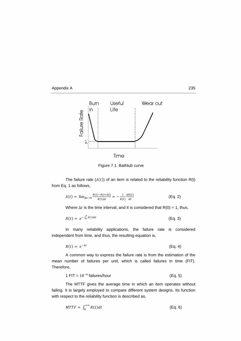
Appendix A 235

The failure rate (𝜆(𝑡)) of an item is related to the reliability function R(t) from Eq. 1 as follows,

𝜆(𝑡) = limΔ𝑡→0𝑅(𝑡)−𝑅(𝑡+∆𝑡)

𝑅(𝑡)∆𝑡= − 1

𝑅(𝑡)𝑑𝑅(𝑡)𝑑𝑡

(Eq. 2)

Where ∆𝑡 is the time interval, and it is considered that R(0) = 1, thus,

𝑅(𝑡) = 𝑒−∫ 𝜆𝑡0 (𝜏)𝑑𝜏 (Eq. 3)

In many reliability applications, the failure rate is considered independent from time, and thus, the resulting equation is,

𝑅(𝑡) = 𝑒−𝜆𝑡 (Eq. 4)

A common way to express the failure rate is from the estimation of the mean number of failures per unit, which is called failures in time (FIT). Therefore,

1 FIT = 10−9 failures/hour (Eq. 5)

The MTTF gives the average time in which an item operates without failing. It is largely employed to compare different system designs. Its function with respect to the reliability function is described as,

𝑀𝑇𝑇𝐹 = ∫ 𝑅(𝑡)𝑑𝑡+∞0 (Eq. 6)

Figure 7.1. Bathtub curve

236 Reliability Engineering

If the failure rate is considered constant in time, the MTTF is 1/𝜆. The MTTR is the mean time it takes to fully restore the system to a given state. It depends on the maintainability of the item, such as proper fault diagnosis, replaceable components, etc.

Finally, availability is defined as the probability that a system will be functioning at a given time. If the system is repaired each time to an “as good as new” state, the average availability is,

𝐴𝑣𝑎𝑖𝑙𝑎𝑏𝑖𝑙𝑖𝑡𝑦 = 𝑀𝑇𝑇𝐹𝑀𝑇𝑇𝐹+𝑀𝑇𝑇𝑅

(Eq. 7)

As a result, increasing the MTTF and decreasing MTTR improves availability, and for industrial applications, this means an increase of production. In the previous statements, we have considered the failure rate as a given parameter; however, it has been a major historical issue the discovery of this quantity. Indeed, reliability prediction has become an engineering subject itself.

While some people view reliability prediction as art more than science, others think they are useless or dangerous, and still others believe them to be indispensible to understanding reliability and formulating safety and business decisions. A major reason for these disparate views is the inconsistency among prediction methods, lack of proper documentation for the processes, and failure to quantify data sources and uncertainties [1].

First attempts to reduce the uncertainty and improve reliability prediction were based on reliability handbooks. They are employed for components showing constant failure rates. The failure rates are given summarized on tables arranged by part type. Multiplicative factors are provided depending on the environmental conditions to which the system is submitted. Therefore, in order to make a prediction, a complete description of the hardware is required. It is also required to know the intended functions and the operating and environmental conditions. The term given for the description of the operating and environmental conditions that the system must endure is mission profile. The mission profile will vary depending on the application, i.e. it will not be the same mission the one assigned to a space shuttle, than the one of a road vehicle. The common mission profile adopted for road vehicles in Europe has been the New European Driving Cycle (NEDC) (Figure 7.2). It shows the variation of the speed with respect to travel time for a typical journey of

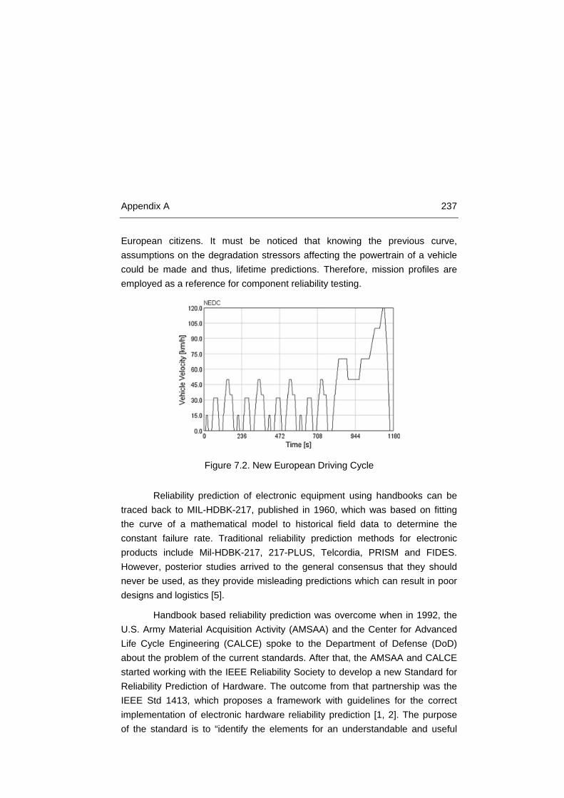
Appendix A 237

European citizens. It must be noticed that knowing the previous curve, assumptions on the degradation stressors affecting the powertrain of a vehicle could be made and thus, lifetime predictions. Therefore, mission profiles are employed as a reference for component reliability testing.

Reliability prediction of electronic equipment using handbooks can be traced back to MIL-HDBK-217, published in 1960, which was based on fitting the curve of a mathematical model to historical field data to determine the constant failure rate. Traditional reliability prediction methods for electronic products include Mil-HDBK-217, 217-PLUS, Telcordia, PRISM and FIDES. However, posterior studies arrived to the general consensus that they should never be used, as they provide misleading predictions which can result in poor designs and logistics [5].

Handbook based reliability prediction was overcome when in 1992, the U.S. Army Material Acquisition Activity (AMSAA) and the Center for Advanced Life Cycle Engineering (CALCE) spoke to the Department of Defense (DoD) about the problem of the current standards. After that, the AMSAA and CALCE started working with the IEEE Reliability Society to develop a new Standard for Reliability Prediction of Hardware. The outcome from that partnership was the IEEE Std 1413, which proposes a framework with guidelines for the correct implementation of electronic hardware reliability prediction [1, 2]. The purpose of the standard is to “identify the elements for an understandable and useful

Figure 7.2. New European Driving Cycle

238 Reliability Engineering

reliability prediction”, so that a prediction in compliance with the standard will identify critical pieces of information necessary for a user of the prediction to determine the accuracy, uncertainty, and, ultimately, value of the prediction.

All in all, apart from reliability predictions, different methodologies have been proposed in order to develop items with high reliability and safety levels. Not only it is taken into account the final item lifetime prediction, but it is influenced throughout the whole development process (lifecycle) of the item to obtain a certain degree. One of these is the Reliability, Availability, Maintainability and Safety (RAMS) methodology. Largely employed in the railway industry for safety critical applications, it is the fundamental of several standards. The aim of these standards is not setting availability, reliability or maintainability targets, but to address the system itself, including test and assessment requirements, and associated tasks and documentation.

One of the key points is the design of failure analysis, trying to anticipate them and mitigate the consequences of hazardous events. To derive the requirements in an effective manner, system engineering-based risk assessment and mitigation logic are used. Widely employed tools addressing failure and risk discovery are: Reliability Hazard Analysis (RHA), Fault Tree Analysis (FTA), Failure Mode and Effects Analysis (FMEA), Functional Hazard Analysis (FHA), etc.

One of the reference standards in the automotive industry is the ISO 26262 employed to comply with needs specific to the application of electrical and electronic (E/E) system within road vehicles. At the moment, there is not a specific standard for FEV electric and electronic systems. The standard applies to all activities during the safety lifecycle of safety-related systems. Some of the points content within the standard are shown to serve as a reference.

The ISO 26262 provides,

• an automotive safety lifecycle including: the management, the development, the production, the operation, the service, and even decommissioning;

• an automotive-specific risk-based approach to determine integrity levels (Automotive Safety Integrity Levels (ASIL));

Appendix A 239

• uses ASIL to specify applicable requirements to avoid unreasonable residual risks;

• requirements for validation and confirmation measures to ensure an acceptable risk level;

• requirements for relations with suppliers.

7.2 References [1] “IEEE Standard Framework for Reliability Prediction of Hardware," in IEEE Std

1413-2010 (Revision of IEEE Std 1413-1998), pp.1-20, April 9 2010

[2] “IEEE Guide for Selecting and Using Reliability Predictions Based on IEEE 1413," in IEEE Std 1413.1-2002, vol., no., pp.0_1-, 2003

[3] P.D.T. O’Connor “Practical Reliability Engineering”, Wiley Online Library, 4th Edition, 2004, ISBN: 0-470-84463-9

[4] Pecht, M (1995) “Product Reliability, Maintainability, and Supportability Handbook”, CRC Press, ARINC Research Corporation, ISBN: 0-8493-9457-0

[5] M. J. Cushing, D.E. Mortin, T.J. Stadterman, and A. Malhotra, “Comparison of Electronics-Reliability Assessment Approaches,” IEEE Transactions on Reliability, Vol. 42, no. 4, pp. 542-546, 1993

8 II. Appendix B: FEV RAMS

Analysis

An important task of reliability engineering is risk and hazards events assessment in case of failure of the systems, in order to counteract and diminish its negative effects. Reliability, Availability, Maintainability and Safety (RAMS) analysis is an efficient tool to discover and assess these critical functional failures. A RAMS analysis of the FEV powertrain was developed in the HEMIS project, in which the author was involved, and expert knowledge was required for criticality assessment of the failures. The reader can enlarge the content of this chapter accessing the public deliverables of the project (www.hemis-eu.org) available until 2019. Here, a brief introduction and a general idea of the methods employed is presented.

The final point of this Appendix deals with the theory of Monte-Carlo Simulations. Monte-Carlo simulations have been employed for reliability and availability analysis in safety critical applications, such as, nuclear power plants and aerospace systems. Monte Carlo simulations were employed in order to assess the improvement on Reliability and Availability when installing a PHMS on a FEV. The results are found on the publications Appendix within the conference paper called “Assessment of the improvement of the safety and reliability embedding an Electrical Powertrain Health Monitoring in a FEV”, by B. Sedano et al.

242 FEV RAMS Analysis

8.1 Introduction Reliability, Availability, Maintainability and Safety (RAMS) techniques

have been extensively applied to the electro-technical engineering field. RAMS techniques allow reliability engineers to forecast failures from the observation of operational field data [6, 16]. This study considers the possible applications of RAMS techniques to the case of FEV functional failures, focusing on the FEV powertrain.

RAMS analysis is well-structured, usually based on standards and follows systematic procedures. Different steps are required prior to the RAMS analysis, which are, the definition of the architecture of a generic FEV, the preliminary hazards analysis (PHA), the establishment of a tolerable hazard rate, the definition of safety goals, and finally, carrying out the RAMS analysis and apportionment. In this case, a Monte-Carlo simulation was also run to assess the improvement of reliability with the implementation of the PHM system as a risk reduction methodology.

The reference standard in automotive industry for electric and electronic (E/E) systems design within road vehicles, the ISO 26262, sets the steps through the whole lifecycle of a product. The so-called V development model (Figure 8.1) is employed, which comprises different actions to be followed during each phase of the lifecycle. It also establishes the tolerable hazard rate of new systems depending on the required safety level.

Following the V model implicit in ISO 26262, the risk analysis of a new system belongs to the concept phase. One way to analyze it is through the RAMS analysis. The purpose of the RAMS analysis is to assess and determine the most critical components within a system and its relationships with respect to the functional safety.

Appendix B 243

The next points are followed for the development of a RAMS analysis, the definition of a generic architecture, the development of a Preliminary Hazard Analysis (PHA) and finally, the RAMS apportionment is developed through established tools, such as FTA, FMECA and Ishikawa diagrams employed for failure criticality analysis. First of all, the tolerable hazard rate must be assigned with respect to the ASIL levels.

8.1.1 Tolerable Hazard Rate assignment to ASIL The approach for probabilistic Safety Integrity Level (SILs) can be found

in a number of standards, depending on the environment, such as EIC 61508 (generic), IEC 61513 (nuclear power), IEC 62061 (machinery), and EN 50129 (railway). These domains rely on the concept of safety functions as a mechanism of risk reduction. For the automotive industry, however, safety functions are not easily distinguished from non-safety functions. Hence in ISO 26262, which is the automotive interpretation of IEC 61508, no quantitative targets are associated with the ASILs.

The tolerable hazard rate (THR) is a rate of occurrence of dangerous events that is deemed to be acceptable from a piece of equipment in order to achieve overall safety targets. Although this concept is used in EN 50129, THR in the form of quantified safety targets for each particular railway application are

Figure 8.1. ISO 26262 V Process model

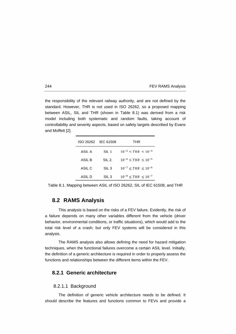
244 FEV RAMS Analysis

the responsibility of the relevant railway authority, and are not defined by the standard. However, THR is not used in ISO 26262, so a proposed mapping between ASIL, SIL and THR (shown in Table 8.1) was derived from a risk model including both systematic and random faults, taking account of controllability and severity aspects, based on safety targets described by Evans and Moffett [2].

ISO 26262 IEC 61508 THR

ASIL A SIL 1 10−5 ≤ 𝑇𝐻𝑅 ≤ 10−4

ASIL B SIL 2. 10−6 ≤ 𝑇𝐻𝑅 ≤ 10−5

ASIL C SIL 3 10−7 ≤ 𝑇𝐻𝑅 ≤ 10−6

ASIL D SIL 3 10−8 ≤ 𝑇𝐻𝑅 ≤ 10−7

Table 8.1. Mapping between ASIL of ISO 26262, SIL of IEC 61508, and THR

8.2 RAMS Analysis This analysis is based on the risks of a FEV failure. Evidently, the risk of

a failure depends on many other variables different from the vehicle (driver behavior, environmental conditions, or traffic situations), which would add to the total risk level of a crash; but only FEV systems will be considered in this analysis.

The RAMS analysis also allows defining the need for hazard mitigation techniques, when the functional failures overcome a certain ASIL level. Initially, the definition of a generic architecture is required in order to properly assess the functions and relationships between the different items within the FEV.

8.2.1 Generic architecture

8.2.1.1 Background

The definition of generic vehicle architecture needs to be defined. It should describe the features and functions common to FEVs and provide a

Appendix B 245

general overview. The relationships between the functions should also be included.

The generic electric vehicle architecture that is proposed must therefore reflect a balance between the desire to make the analysis generic (and therefore high level) whilst also considering sufficient detail to make the RAMS analysis practicable. It is anticipated that the architecture may need to be further developed in the course of the RAMS analysis activities.

Some assumptions must be made about the nature of the vehicle in order to describe the architecture at a level that is suitable for analysis. Firstly, it is assumed that the target application is probably a near-future, high-end passenger vehicle. Although the physical and electrical architectures of alternative powertrain vehicles vary widely, the focus is “fully electric vehicles” (FEVs). In the context of the European Green Cars Initially, FEVs are defined [6] as:

• electrically-propelled vehicles that provide significant driving range on purely battery-based power.

• including vehicles with range extenders. • including small light-weight passenger and light duty vehicles.

The FEV concept therefore includes series hybrid architectures and vehicles equipped with other energy sources such as fuel cells, as well as the purely battery powered.

At subsystem level many options and technologies are available. Electrical machines are available in many topologies: examples used in automotive traction applications include induction, DC brushed, synchronous permanent magnet, and synchronous brushed motors. Switched reluctance machines are also under investigation for automotive traction applications. Power ratings for automotive traction machines range from less than 5 kW to more than 200 kW for electric and hybrid electric passenger cars [3]. Traction currents are delivered in DC form between energy sources and inverters, but in three-phase form between machines and inverters.

Similarly, a wide variety of operating voltages (up to 650 V [4]) and cell chemistries (e.g. lead acid, lithium ion, nickel metal hydride) have also been deployed for automotive traction applications.

246 FEV RAMS Analysis

Consequently, the initial assumptions that have been made concerning the electric powertrain are:

• traction power will be provided only via PMSM electrical machines, and not mechanically from any on-board energy generator (such as an ICE);

• the electrical machine could be operated as a traction motor, or as a generator under braking conditions;

• the vehicle could contain at least one such machine, but possibly more (e.g. one in each wheel, or one for each axle).

• electrical energy storage is provided by a high voltage traction battery, as this is the most commonly used solution;

• energy may be obtained from the following sources: o the electricity grid (by conductive or inductive charging – note

that the latter may be achieved by wireless power transfer, during which the vehicle may active but temporarily stationary above a source coil embedded in the road, or possibly even while in motion);

o energy recovery during regenerative braking; o possibly from an on-board energy generator (which could be an

ICE or turbine coupled to a generator, or a fuel cell system generating electricity).

8.2.1.2 Definition

The generic electric vehicle architecture that is proposed must therefore reflect a balance between the desire to make the analysis generic (and therefore high level) whilst also considering sufficient detail to make the RAMS analysis practicable.

As it is not practicable to address the entire vehicle, this analysis focuses on those elements of the system that are important for the PHMS and the electric powertrain components that this system is intended to monitor.

8.2.1.2.1 Functional view

A functional view of the adopted vehicle architecture is illustrated in Figure 8.2, which focuses on those elements of the vehicle that are important

Appendix B 247

for the PHM system and the electric powertrain functions. In Figure 8.2 the Powertrain Domain is shown in great detail. Relevant interfaces, both internal and external to the vehicle, are also shown.

Interfaces between the vehicle systems and the driver are split into four

groups, depending on which of the functional domains is involved. These are:

• Driver Interfaces: Representing interactions via the Instrument Panel with the Body Electronics Domain (driver inputs include controls for climate, window position, lighting etc.)

• Driving Demand: Representing driver input to functions associated with the Chassis and Safety Domain, indicated by the steering wheel, brake pedal and ACC selector switches.

• Powertrain Demand: Representing Driver input to functions associated with the Powertrain Domain, indicated by the Driver via the accelerator pedal and the PNRD selector. Sensor signals

Figure 8.2. Generic electric vehicle architecture: functional view

Functional DomainsEnergySystem

HV TractionBattery

Electrical Transmission

Auxiliary LV Battery

Vehicle

Mechanical Transmission

HEMIS PHMS EM Field Monitor

LV SourceBus

HV DC Power Bus

LV DC Power Bus

INFOTAINMENT

BODY ELECTRONICS

Pedal and Direction Sensors

Transmission Sensors

TransmissionMechanicalThermalHigh voltage (HV)Low voltage (LV)Signals/DataGas

Environment

Wheels

Diagnostic Systems

Radiator

Nearby Vehicles

Vehi

cle

Back

bone

Net

wor

k

ControlHV AC

Power Bus

Electrical Machine

HV DCSourceBus Braking

System

Steering

DC/DC Converter

ACC System

Steering Sensors

ChassisSensors

External Networks

Communications Antennas

Driving Demand

Diagnostic Interface

ACC Radar Antenna

ExhaustAir Intake

On-board Energy Source

ChargingSystem

Instrument Panel

CHASSIS AND SAFETY

COMMUNICATIONS

Driver

ThermalBus

Atmosphere

Road

Infotainment Interfaces

ChargingPower

Interface

Charging Data

Interface

Vehicle Charging Station Passengers

POWERTRAIN

Powertrain Controller

Powertrain Domain Network

Powertrain Thermal Management

Analysis & WarningBattery Management

System

ThermalBus

Powertrain Demand

Driver Interfaces

248 FEV RAMS Analysis

reflecting the pedal positions and PNRD selector status are made available on the Powertrain Domain Network.

• Infotainment Interfaces: Mechanisms for receiving input from the Driver and the Passengers and providing infotainment services to the Driver and Passengers.

A deeper analysis of electrical transmission is required for a proper assessment of the failures. In this sense, the components belonging to the electrical transmission were further extended.

8.2.1.3 Electrical Transmission

A more refined description of the architecture of the Electrical Transmission identified in the generic vehicle architecture is described now.

8.2.1.3.1 Electrical Transmission Architecture

The generic Electrical Transmission, illustrated in Figure 8.3, includes one or more traction machines, power electronics to drive the traction machine(s), and local controls for the power electronics. Associated components include the HV DC Power Bus connecting the Electrical Transmission to the Energy System, the HV AC Power Bus connecting the traction machine to the power electronics, and various sensors that provide status information for control and monitoring of the traction machine and power electronics.

In the analysis that follows the HV AC Power Bus is regarded as part of the Electrical Machine, and the HV DC Power Bus is regarded as part of the Inverter.

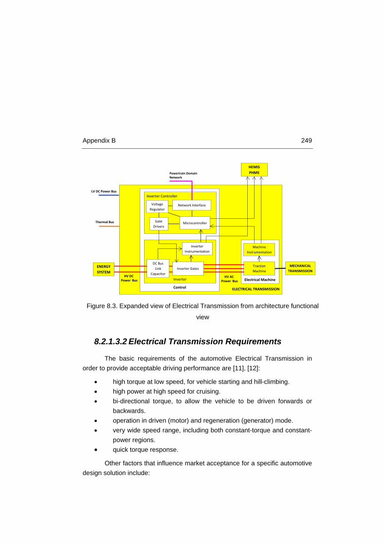
Appendix B 249

8.2.1.3.2 Electrical Transmission Requirements

The basic requirements of the automotive Electrical Transmission in order to provide acceptable driving performance are [11], [12]:

• high torque at low speed, for vehicle starting and hill-climbing. • high power at high speed for cruising. • bi-directional torque, to allow the vehicle to be driven forwards or

backwards. • operation in driven (motor) and regeneration (generator) mode. • very wide speed range, including both constant-torque and constant-

power regions. • quick torque response.

Other factors that influence market acceptance for a specific automotive design solution include:

Figure 8.3. Expanded view of Electrical Transmission from architecture functional

view

ELECTRICAL TRANSMISSIONControl

Electrical MachineInverter

Thermal Bus

LV DC Power Bus

Inverter Gates

HV AC Power Bus

Traction Machine

Powertrain Domain Network

ENERGY SYSTEM

MECHANICAL TRANSMISSION

HEMISPHMS

MachineInstrumentation

InverterInstrumentation

Inverter Controller

MicrocontrollerGate Drivers

Network Interface

HV DC Power Bus

Voltage Regulator

DC Bus Link

Capacitor

250 FEV RAMS Analysis

• high efficiency over wide speed and torque ranges, as well as when used as a generator (in regenerative mode), in order to minimize energy consumption and maximize vehicle range.

• high reliability and robustness over a wide range of vehicle operating conditions, as well as a degree of fault tolerance in order to ensure customer satisfaction and minimize maintenance requirements.

• high power density (i.e. small size and low weight) in order to simplify vehicle packaging, minimize energy consumption, and maximize range.

• reasonable cost, in order to ensure that the Electrical Transmission is affordable.

Different machine topologies offer different performance characteristics, as well as limitations that may be both technical and economic. Different machine designs also require different power electronics topologies and control algorithms. Thus, both the type of machine and its associated power converter and control technologies matter on the cost/benefit and performance trade-offs that must be carried out for any particular Electrical Transmission design.

8.2.1.4 Electrical Machine components

The carried out analysis aims to be as generic as possible, as it is not focused on a specific vehicle or even a narrow class of vehicles. However, at lower levels of description it becomes necessary to become more specific about the design details. In particular, electric motor/generator designs are wide-ranging and constantly evolving.

A view showing decomposition of a generic Traction Machine is shown in Figure 8.4, which illustrates its lower level subsystems.

Appendix B 251

The main differences between different motor types relate to the implementation of the Rotor Magnetic Field Source, here we consider the Permanent Magnet Synchronous Machine (PMSM), provided its high application on automotive drives:

• PMSM: In the PMSM, permanent magnets are used to provide a permanent magnetic field. In drive mode the permanent magnetic field of the rotor magnets interacts with the stator magnetic field (created by drive currents in the Stator Windings), causing the Rotor Shaft to rotate. In regeneration mode, the rotating magnetic field of the spinning Rotor Magnets induces currents in the Stator Windings.

The other components of the Traction Machine are similar for different machine types considered. Consequently, most of the failure mechanisms are also common.

8.2.1.5 Power Electronics components

A view showing the composition of a generic three-phase inverter (DC/AC) is shown in Figure 8.5, illustrating its lower level subsystems.

Figure 8.4. Hierarchical view of generic Traction Machine

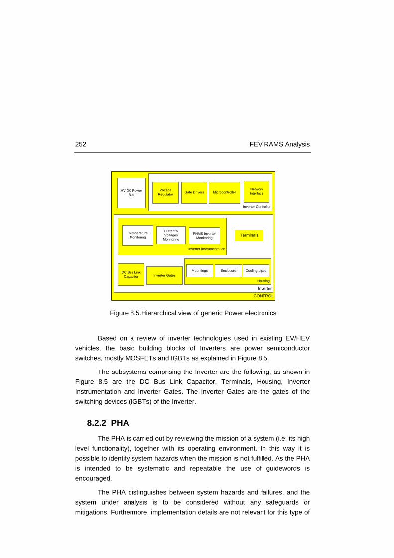
252 FEV RAMS Analysis

Based on a review of inverter technologies used in existing EV/HEV vehicles, the basic building blocks of Inverters are power semiconductor switches, mostly MOSFETs and IGBTs as explained in Figure 8.5.

The subsystems comprising the Inverter are the following, as shown in Figure 8.5 are the DC Bus Link Capacitor, Terminals, Housing, Inverter Instrumentation and Inverter Gates. The Inverter Gates are the gates of the switching devices (IGBTs) of the Inverter.

8.2.2 PHA The PHA is carried out by reviewing the mission of a system (i.e. its high

level functionality), together with its operating environment. In this way it is possible to identify system hazards when the mission is not fulfilled. As the PHA is intended to be systematic and repeatable the use of guidewords is encouraged.

The PHA distinguishes between system hazards and failures, and the system under analysis is to be considered without any safeguards or mitigations. Furthermore, implementation details are not relevant for this type of

Figure 8.5.Hierarchical view of generic Power electronics

CONTROL

HV DC Power Bus

Inverter

Inverter Controller

DC Bus Link Capacitor

Terminals

Inverter Gates

Inverter Instrumentation

Housing

Temperature Monitoring

Currents/Voltages

MonitoringPHMS Inverter

Monitoring

Mountings Enclosure Cooling pipes

Voltage Regulator Gate Drivers Microcontroller

Network Interface

Appendix B 253

study. The defined generic architecture forms the basis of the PHA. The focus of this analysis is to identify hazards.

The high level functions of the systems are specified, based on the architectural description, in order to identify functional failures that could result in hazards. The hazard identification was carried out in two parts: the first part identified hazards related to functional failures of the system; the second part identified non-functional hazards that are inherent in the novel technologies assumed to be used in the vehicle.

The objective of the PHA is to translate system hazards into design constraints, or functional safety requirements. Once the hazards were identified, each was assessed in terms of their potential consequences (“severity”), likelihood of occurrence (“exposure”) and opportunities for the driver to influence the outcome (“controllability”). A risk graph is then used in order to establish and classify the associated risks in terms of the Automotive Integrity Levels (ASILs)

The preliminary hazard analysis (PHA) is normally carried out by reviewing the mission of a system, i.e. its high level functionality, together with the environment around the system and its uses.

8.2.2.1 Hazard classification

The identified hazards were classified using the ISO 26262 risk criteria [6]0, which are briefly outlined below.

8.2.2.1.1 Severity

The ‘severity’ of potential harm shall be estimated based on a defined rationale for each hazardous event. The severity shall be assigned to one of the severity classes S0, S1, S2 or S3 in accordance with Table 8.2 below.

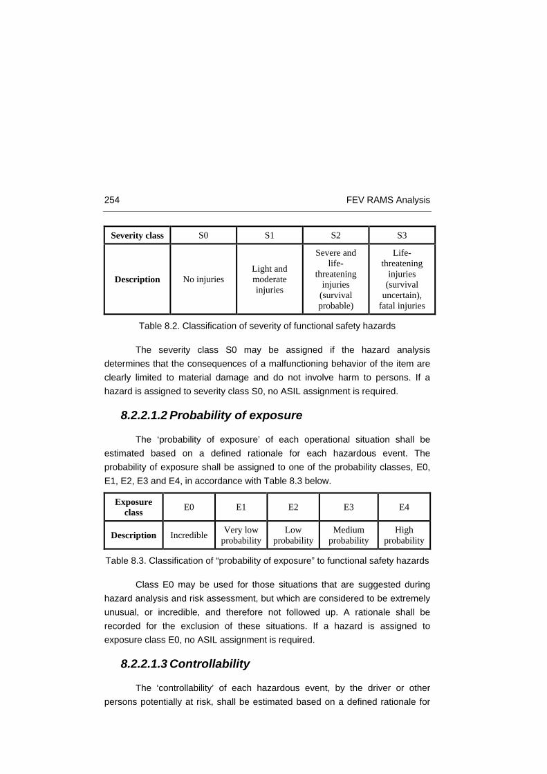
254 FEV RAMS Analysis

Severity class S0 S1 S2 S3

Description No injuries Light and moderate injuries

Severe and life-

threatening injuries

(survival probable)

Life-threatening

injuries (survival

uncertain), fatal injuries

Table 8.2. Classification of severity of functional safety hazards

The severity class S0 may be assigned if the hazard analysis determines that the consequences of a malfunctioning behavior of the item are clearly limited to material damage and do not involve harm to persons. If a hazard is assigned to severity class S0, no ASIL assignment is required.

8.2.2.1.2 Probability of exposure

The ‘probability of exposure’ of each operational situation shall be estimated based on a defined rationale for each hazardous event. The probability of exposure shall be assigned to one of the probability classes, E0, E1, E2, E3 and E4, in accordance with Table 8.3 below.

Exposure class E0 E1 E2 E3 E4

Description Incredible Very low probability

Low probability

Medium probability

High probability

Table 8.3. Classification of “probability of exposure” to functional safety hazards

Class E0 may be used for those situations that are suggested during hazard analysis and risk assessment, but which are considered to be extremely unusual, or incredible, and therefore not followed up. A rationale shall be recorded for the exclusion of these situations. If a hazard is assigned to exposure class E0, no ASIL assignment is required.

8.2.2.1.3 Controllability

The ‘controllability’ of each hazardous event, by the driver or other persons potentially at risk, shall be estimated based on a defined rationale for

Appendix B 255

each hazardous event. The controllability shall be assigned to one of the controllability classes C0, C1, C2 and C3 in accordance with Table 8.4 below.

Controllability class C0 C1 C2 C3

Description Controllable in general

Simply controllable

Normally controllable

Difficult to control or

uncontrollable

Table 8.4. Classification of “controllability” of functional safety hazards

Class C0 may be used for hazards addressing the unavailability of the item if they do not affect the safe operation of the vehicle (e.g. some driver assistance systems). Class C0 may also be assigned if dedicated regulations exist that specify the functional performance with respect to a defined hazard, and C0 is argued using the corresponding existing experience concerning sufficient controllability.

8.2.2.2 Determination of ASIL and safety goals

In ISO 26262 a risk-based approach is presented for determining automotive safety risk classes known as ‘automotive safety integrity levels’ (ASILs).

The ASILs are used for specifying the necessary safety integrity requirements for safety functions that are required to achieve an acceptable level of residual risk. In this scheme, four ASILs are defined: ASIL A, ASIL B, ASIL C and ASIL D; where class D represents the highest integrity category and class A the lowest. In addition to these four ASILs, the class QM (quality management) denotes no requirement to comply with ISO 262622.

The ASIL is determined for each hazardous event using the severity, exposure and controllability parameters, as indicated in Table 8.5 below.

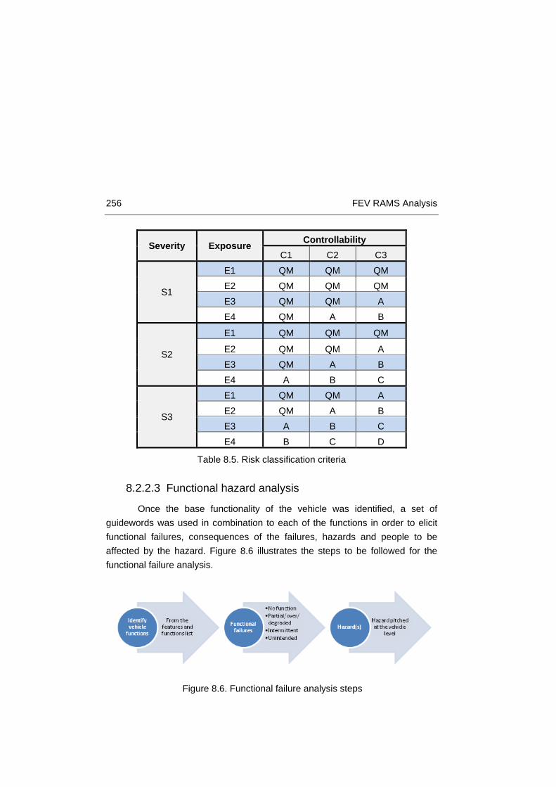
256 FEV RAMS Analysis

Severity Exposure Controllability C1 C2 C3

S1

E1 QM QM QM E2 QM QM QM E3 QM QM A E4 QM A B

S2

E1 QM QM QM

E2 QM QM A E3 QM A B E4 A B C

S3

E1 QM QM A E2 QM A B E3 A B C E4 B C D

Table 8.5. Risk classification criteria

8.2.2.3 Functional hazard analysis

Once the base functionality of the vehicle was identified, a set of guidewords was used in combination to each of the functions in order to elicit functional failures, consequences of the failures, hazards and people to be affected by the hazard. Figure 8.6 illustrates the steps to be followed for the functional failure analysis.

Figure 8.6. Functional failure analysis steps

Appendix B 257

Hazards causes have not been included but these will be identified in the RAMS analysis stage. For each functional failure a hazard title has been consolidated. The identified hazards were classified using the ISO 26262 risk criteria and the classification took into consideration example situations and the most severe outcome was recorded.

8.2.2.4 Hazard analysis and risk classification results

Based on the assumptions about the vehicle architecture and operation, a number of potential safety hazards related to the electrical powertrain were identified that were considered to be the most critical.

The FEV hazards identified for the study are:

• FHAZ_01 – Undemanded acceleration

• FHAZ_02 – Undemanded deceleration

• FHAZ_03 – No vehicle acceleration

• FHAZ_04 – No vehicle deceleration

• FHAZ_05 – Excessive acceleration

• FHAZ_06 – Insufficient acceleration

• FHAZ_07 – Reversed acceleration

• FHAZ_08 – Increased vehicle stopping distance

• FHAZ_09 – Vehicle instability

• FHAZ_10 – Vehicle roll-away

The results of the analysis are summarized in Table 8.6.

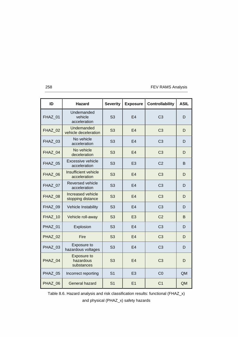
258 FEV RAMS Analysis

ID Hazard Severity Exposure Controllability ASIL

FHAZ_01 Undemanded

vehicle acceleration

S3 E4 C3 D

FHAZ_02 Undemanded vehicle deceleration S3 E4 C3 D

FHAZ_03 No vehicle acceleration S3 E4 C3 D

FHAZ_04 No vehicle deceleration S3 E4 C3 D

FHAZ_05 Excessive vehicle acceleration S3 E3 C2 B

FHAZ_06 Insufficient vehicle acceleration S3 E4 C3 D

FHAZ_07 Reversed vehicle acceleration S3 E4 C3 D

FHAZ_08 Increased vehicle stopping distance S3 E4 C3 D

FHAZ_09 Vehicle Instability S3 E4 C3 D

FHAZ_10 Vehicle roll-away S3 E3 C2 B

PHAZ_01 Explosion S3 E4 C3 D

PHAZ_02 Fire S3 E4 C3 D

PHAZ_03 Exposure to hazardous voltages S3 E4 C3 D

PHAZ_04 Exposure to hazardous substances

S3 E4 C3 D

PHAZ_05 Incorrect reporting S1 E3 C0 QM

PHAZ_06 General hazard S1 E1 C1 QM

Table 8.6. Hazard analysis and risk classification results: functional (FHAZ_x)

and physical (PHAZ_x) safety hazards

Appendix B 259

8.2.2.5 Safety goal identification

After the main functional hazards have been identified, a safety goal must be determined for each hazardous event with an ASIL evaluated in the previous hazard analysis. Safety goals are top level safety requirements for the FEV. Safety goals are expressed in terms of functional objectives. The case of undemanded vehicle acceleration is employed as an example.

FHAZ_01: Undemanded vehicle acceleration

Safety goal: The vehicle must not accelerate without valid acceleration demand.

8.2.3 RAMS apportionment RAMS apportionment is the application of the RAMS techniques to

deeply investigate the origins of the hazards identified by the PHA. In this sense, Fault Tree Analysis (FTA), Failure Mode Effects and Criticality Analysis (FMECA) and Ishikawa diagrams are employed.

It must be noted that the RAMS apportionment for the FEV powertrain was developed leaving aside the battery. Much research is being developed on battery degradation analysis [19, 20] and there are specific projects focused solely on FEV batteries, including new chemistries development. As a consequence, the failure modes affecting the electric machine and the inverter were addressed for the detected functional hazards.

8.2.3.1 FTA

Fault Tree Analysis (FTA) is a top-down approach to the failure analysis, starting from any potential adverse event and then setting out all the ways the event can happen. The analysis includes functionality, failure definition, architecture, and stress and operational profiles. It provides a methodical way of following the functional flow of products down to the low level assemblies, components, failure modes, and respective causes of events and their combinations. Flexibility of modeling of various functional conditions and interaction such as enabling events, events with specific priority of occurrence, etc. using FTA, provides for accurate representation of the interdependence of the functionality of the product.

260 FEV RAMS Analysis

A fault tree is a logic diagram that displays the interrelationships between a potential critical event (accident) in a system (i.e. a FEV), and the reasons for this event.

This logic diagram is a graphical model illustrating the state of the system’s subsystems (basic events), and the connections between these basic events and the system’s state (TOP event). The graphical symbols used to illustrate these connections are called ‘logic gates’. The output from a logic gate is determined by the input events.

SYMBOL LOGIC GATE NAME DESCRIPTION

AND gate

The ‘AND’ gate indicates that the

output event occurs if all of the

input events occurs simultaneously

OR gate

The ‘OR’ gate indicates that the

output event occurs if any of the

input events occurs

PASS-THROUGH gate The ‘PASS-THROUGH’ gate

Description of STATE The comment rectangle is for

supplementary information

BASIC event

The ‘Basic’ event represents a

basic equipment fault or failure

that requires no further

development into more basic faults

or failures

TRANSFER

The ‘Transfer’ symbol indicates

that the fault tree is developed

further at the occurrence of the

corresponding ‘Transfer’ symbol

Table 8.7. Fault Tree Symbols

Appendix B 261

Table 8.7 shows the most commonly used fault tree symbols, together with a brief description of their interpretation.

The fault tree analysis (FTA) is based on the previous FEV architecture definition and on the hazards defined in the preliminary hazard analysis (PHA), not considering the hazards assessed class QM (quality management) which denotes no requirement to comply with ISO 262622.

The undemanded vehicle acceleration fault tree is shown as an example in Figure 8.7.

Figure 8.7. Undemanded vehicle acceleration fault tree

Undemanded acceleration

Failure in Powertrain

Domain

Failure in Electrical

Transmission

Failure in Control

Failure in Electrical Machine

Failure in Inverter

Failure in Inverter

Controller

Fault Control of Inverter

Controller

Software failure

Hardware failure

Spurious current from

inverter

Failure in Microcontroller

262 FEV RAMS Analysis

8.2.3.2 FMECA

Following the V model implicit in ISO 26262 the FMEA belongs to the concept phase.

Failure Mode, Effects and Criticality Analysis (FMECA) is a bottom-up, inductive analytical method which studies the effects of single component or function failures on the system or subsystem. It is useful for exhaustive listing of all potential initiating faults. FMECA is a safety engineering technique aimed at identifying and classifying potential failure modes, their effect on the system and defining actions to avoid these failures. Its main use is to classify the effect of potential failure modes by severity, occurrence and detection and subsequently prioritize the actions needed to counteract or avoid these failures. This is done by calculating the risk priority numbers (RPN) for each failure mode. The Risk Priority Number (RPN) is computed as a simple product of the Severity, Occurrence and Detection ratings: RPN = Severity × Occurrence × Detection.

This value may then be used to prioritize the failure modes that require a corrective action. If the Risk Priority Number (RPN) is less than 35, actions must be recommended to counteract or avoid these failures. It should be noted that the ‘severity’ used here is similar but not identical to the severity parameter used in the hazard analysis. The FMECA analysis table results for the inverter most critical components are shown as reference in Table 8.8.

Appendix B 263

FMECA_ID

Subsystem and

Functions

Failure Mode

Causes Subsystem Effect

System Effect

Hazard at vehicle

level

Haz_ID S O D RPN Recommend Actions

2.5.1.1.1 DC Bus Link Capacitor

FMPWT_14/12/16

Stabilize HV DC Power Bus

Increased ripple

Thermal stress, self-heating

Low DC voltage

Poor efficiency. Batteries may get damaged

Insufficient vehicle acceleration / instability

FHAZ_09/06

3 1 3 9 PHMS measures capacitor variables

2.5.1.1.2 Inverter Gates

FMPWT_14/12/16

Switch the IGBTs to chop the DC current

Short circuit

Aging, overloads

Gate driver cut the current flow

Rotor may block

Undemanded vehicle deceleration / No vehicle acceleration

FHAZ_02/03

1 1 2 2 PHMS measures IGBTs internal variables

FMPWT_12/11/2

Loss of gate control

Time dependent breakdown, hot electrons

IGBT will burn out

Rotor may block

Undemanded vehicle deceleration / No vehicle acceleration

FHAZ_02/03

1 1 2 2 PHMS measures IGBTs internal variables

FMPWT_12/11

Burn out latch-up IGBT will burn out

Rotor may block

Undemanded vehicle deceleration / No vehicle acceleration

FHAZ_02/03

1 1 2 2 PHMS measures IGBTs internal variables

FMPWT_12/11/17

Open circuit

Bond wire lift off, solder fatigue

IGBT will overheat

Rotor may block. Motor will work in unsteady way

Instability / No vehicle acceleration

FHAZ_09/03

1 2 3 6 PHMS measures IGBTs internal variables

Table 8.8. FMECA sample of electrical transmission inverter components

264 FEV RAMS Analysis

8.2.3.3 Ishikawa Diagrams

The Ishikawa Diagram [5] (also described as Fishbone Diagram or Cause and Effect Diagram) is a tool that helps in the identification of the root causes of a problem. It provides an overview of the causes of a problem, using a structured representation of all causes that could contribute to produce the undesirable effect. This approach results in a graphical representation of the relationships between all of the potential causes from which one is more readily able to identify the root causes of the problem.

Major benefits of the Ishikawa diagram approach are that it reduces the risk of missing some causes in the analysis, provides a convenient mechanism for documenting the results of the analysis, and acts as an input for further study of potential solutions. This method makes it possible to identify causes, correct defects and provide solutions by employing corrective actions.

The basic structure of the Ishikawa diagram, shown in Figure 8.8, consists of a horizontal primary arrow that is directed towards the problem. Potential causes are sorted into groups that are represented with secondary arrows that terminate on the primary arrow.

Lower-level causes associated with each of the main groups are indicated by smaller horizontal arrows that terminate on the corresponding secondary arrow, with further levels of detail added as necessary in a similar manner. All potential causes are required, from which the real root causes of the problem must be sought, thus allowing corrective solutions to be proposed.

Figure 8.8. Structure of Ishikawa diagram

PROBLEM

Material MachineMeasurement

Manpower Milieu Method

Primary arrow

Secondary arrow

Causecategory

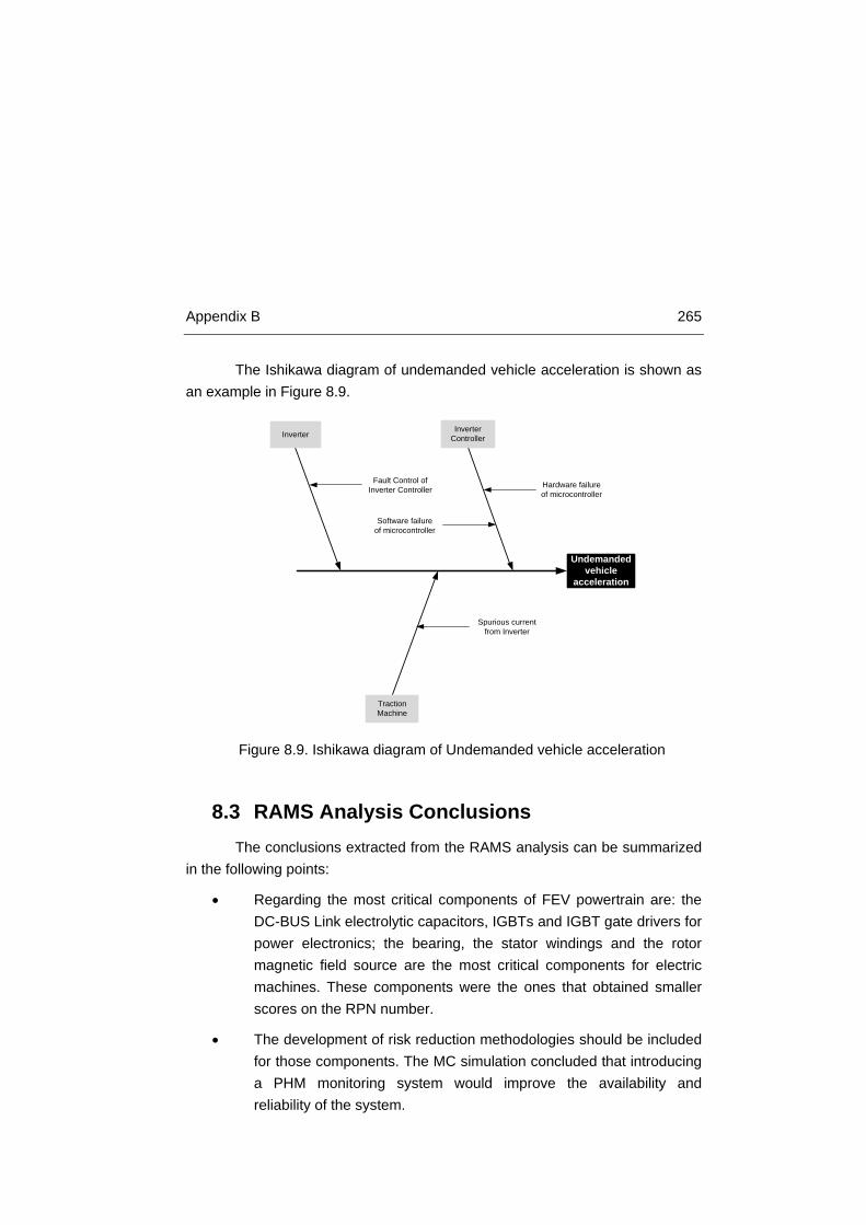
Appendix B 265

The Ishikawa diagram of undemanded vehicle acceleration is shown as an example in Figure 8.9.

8.3 RAMS Analysis Conclusions The conclusions extracted from the RAMS analysis can be summarized

in the following points:

• Regarding the most critical components of FEV powertrain are: the DC-BUS Link electrolytic capacitors, IGBTs and IGBT gate drivers for power electronics; the bearing, the stator windings and the rotor magnetic field source are the most critical components for electric machines. These components were the ones that obtained smaller scores on the RPN number.

• The development of risk reduction methodologies should be included for those components. The MC simulation concluded that introducing a PHM monitoring system would improve the availability and reliability of the system.

Figure 8.9. Ishikawa diagram of Undemanded vehicle acceleration

Undemanded vehicle

acceleration

InverterInverter

Controller

Traction Machine

Fault Control of Inverter Controller

Software failure of microcontroller

Hardware failure of microcontroller

Spurious current from Inverter

266 FEV RAMS Analysis

8.4 Monte-Carlo simulations theory As it was previously point out Monte-Carlo simulations were developed

to assess the improvement on Reliability and Availability of the FEV powertrain when introducing a PHMS. Here, the theory of Monte-Carlo simulations is explained for further understanding the work done on the publication.

Monte-Carlo simulations are extensively employed for complex system reliability and availability modeling [1]. In Monte-Carlo simulations, a logical model of the system being analyzed is repeatedly evaluated, using each run different values of the distributed parameters.

8.4.1.1 Theory

At the initial phase of the design process of a system, the engineer tries to anticipate to the possible problems and future realities of operation the system will be subjected to. Therefore, the engineer looks at a model, rather than at reality itself. By definition a model will never fit reality in all details; it will be at some “distance” from it. The model is based on the available information, the interactions between the elements and with the environment, the properties of components and how they move among their possible states. Once the model is established, questions can be asked about the future expected performance. It is at this point when mathematics comes into play [11].

Monte Carlo method is a powerful tool for the analysis of complex systems, owing to its capability of achieving a closer adherence to reality. It may be defined as a methodology for obtaining estimates of the solution of mathematical problems by means of random numbers sampling. By random numbers we mean numbers obtained through the roulette-like machine of the kind employed in gambling casinos at Montecarlo Principate, thus, the name comes after it. MC method can yield solutions to complex multidimensional problems; however, its employment has been limited to nuclear applications, mainly, due to its requirement for computer memory and time [8].

The MC approach is based on the sampling of random numbers from a given probability distributions (i.e. uniform, exponential, weibull, etc.).

Let 𝑋 ∈ (−∞, +∞) be a real number with cumulative density function (cmd) Fx(x) and probability density function fx(x),

Appendix B 267

𝐹𝑥(𝑥) = ∫ 𝑓𝑥(𝑥′)𝑑𝑥′𝑥−∞ = Pr𝑋 ≤ 𝑥 (Eq. 1)

Thus, through the application of the inverse transform of the corresponding extracted number, knowing the cumulative density function, it is possible to derive when the transition of a given state happens. Since Fx(x) is a non decreasing function, for any y ∈ [0,1), its inverse may be defined as,

𝐹𝑥−1(𝑦) = inf 𝑥:𝐹𝑥(𝑥) ≥ 𝑦 (Eq. 2)

This is a fundamental relationship of the inverse transform method which for any R value sampled from a distribution UR[0,1) gives the corresponding X value sampled from the Fx(x) distribution. The previous is shown in Figure 8.10.

𝑅~𝑈𝑅(𝑟) = 𝑟 𝑖𝑛 [0,1) → 𝑋~𝐹𝑥(𝑥) (Eq. 3)

Taking into account the previous definition, random number sampling can be applied to the system transport problem. Let us consider a system whose states are defined by the values of a set of variables, i.e. by a point P in the phase space Ω. Let us suppose that the evolution of the system is a stochastic process. Each of the possible trajectories of P is then a function of the ensemble generated by the process and the system’s dynamics can be studied by calculating the ensemble values of the quantities of interest, for example probability distributions and expected values.

The Monte Carlo method allows us to generate the sample function of the ensemble: every Monte Carlo history simulates a trajectory of P, in the course of which we accumulate quantities of interest in appropriate counters. At

Figure 8.10. Inverse transform method: continuous distribution

268 FEV RAMS Analysis

the end of the simulation, after a great deal of histories has been generated, the arithmetic averages of the desired quantities represent the Monte Carlo ensemble estimates of the quantities themselves [10-18]. These quantities represent the estimated reliability and availability of the system throughout its whole lifecycle following the studied model.

8.5 References [1] Patrick D. T. O’Connor (2004) “Practical Reliability Engineering”, Wiley Online

Library, 4th Edition, ISBN: 0-470-84463-9

[2] Evans R. Moffett J.D., “Derivation of Safety Targets for the Random Failure of Programmable Vehicle Based Systems”, Proceedings of the 19th International Conference on Computer Safety, Reliability and Security, 240-249, Springer-Verlag Lodon UK, 2000.

[3] J. de Santiago et al., “Electrical motor drivelines in commercial all-electric vehicles: a review”, IEEE Transactions on Vehicular Technology, Vol. 61, No. 2, February 2012, pp. 475–484.

[4] G. Schmid, R. Überbacher and P. Göth, “ELF and LF magnetic field exposure in hybrid- and electric cars”, Proc. Bio-electromagnetics Conf. 2009, Davos, Switzerland, June 2009, Paper 9–3.

[5] K. Ishikawa, “Introduction to Quality Control”, 3A Corporation, Tokyo, 1990.

[6] ISO 26262, Road Vehicles – Functional Safety, November 2011 (parts 1-9); ISO 26262-10 Guideline, July 2012.

[7] B. Sedano, A. R. Ruddle, I. Unanue, L. Low, D. Astigarraga, I. Ibarra, I. Cerro and A. Galarza, "HEMIS: Electrical Powertrain Health Monitoring for Increased Safety of FEVs, Chemical Engineering Transactions," vol. 33,

[8] E. Zio, The Monte Carlo Simulation Method for System Reliability and Risk Analysis, Springer London. Springer London, 2013,

[9] P. Baraldi, F. Barbisotti, R. Capanna, S. Colombo, M. Rigamonti and E. Zio, "Assessment of the Performance of a Fully Electric Vehicle Subsystem in Presence of a Prognostic and Health Monitoring System," Chemical Engineering Transactions, pp. 787, 2013.

[10] E. Zio, "The challenges of system health management and failure prognostics, IEEE Reliability Society 2008 Annual Technology Report," 2008.

Appendix B 269

[11] E. Zio, P. Baraldi and E. Patelli, "Assessment of the availability of an off-shore installation by Monte Carlo simulation, International Journal of Pressure Vessels and Piping," vol. 83 (4), pp. 321-320, 2006

[12] E. D. Cashwell, C.J. Everett, “A practical manual on the Monte Carlo method for random walk problems”, Pergamon Pree, N.Y., 1959.

[13] R.Y. Rubinstein, “Simulation and the Monte Carlo method”, Wiley, 1981.

[14] M.H. Kalos, P.A. Whitlock, “Monte Carlo methods. Volume I: basics”, Wiley, 1986

[15] I. Lux, L. Koblinger, “Monte Carlo particle transport methods: neutron and proton calculations”, CRC Press, 1991.

[16] E.J. Henley, H. Kumamoto, “Probabilistic Risk Assessment”, IEEE Press, 1991

[17] A. Dubi, “Monte Carlo Applications in systems Engineering”, Wiley, 1999

[18] M. Marseguerra, E. Zio, “Basic of the Monte Carlo Method with Application to System Reliability”, LiLoLe-Verlag GmbH (Pbl. Co. Ltd.), 2002

[19] F. Rufus Jr., S. Lee, A. Thakker, “Health Monitoring Algorithms for Space Applications Batteries”, in International Conference on Prognostics and Health Management 2008, 2008.

[20] C. Chen, M. Pecht, “Prognostics of Lithium-Ion Batteries Using Model-Based and Data-Driven Models”, in Prognostics and System Health Management Conference, IEEE, 2012

9 III. Appendix C: Ensemble

method uncertainty

assessment

The methodology to assess the uncertainty accounting the RUL predictions which were made through the employment of a “Bagging” ensemble method was studied and deeply analyzed by P. Baraldi, F. Mangili and E. Zio in “Investigation of uncertainty treatment capability of model-based and data-driven prognostic methods using simulated data” published in Reliability Engineering and System Safety. The methodology employed will be exposed and explained.

The problem faced in this Chapter is quantifying the confidence made in equipment RUL predictions. The prognostic task of RUL prediction is affected by large uncertainties. The sources of uncertainty were classified in three:

A. Randomness in the future degradation of the equipment. This intrinsic uncertainty has several causes, such as, the unknown future load profile, and operation and environmental conditions.

B. Modeling error, i.e. inaccuracy of the prognostic model used to perform the prediction. In model-based prognostic approaches, this source takes into account the assumptions and simplifications made

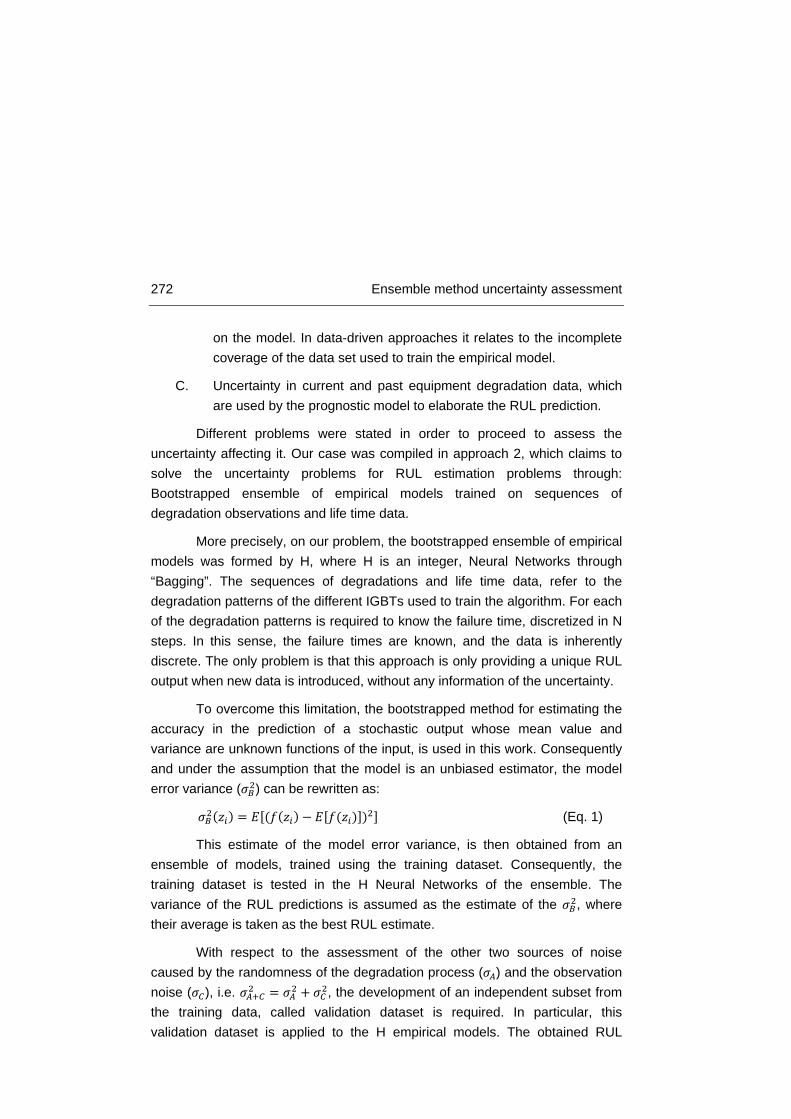
272 Ensemble method uncertainty assessment

on the model. In data-driven approaches it relates to the incomplete coverage of the data set used to train the empirical model.

C. Uncertainty in current and past equipment degradation data, which are used by the prognostic model to elaborate the RUL prediction.

Different problems were stated in order to proceed to assess the uncertainty affecting it. Our case was compiled in approach 2, which claims to solve the uncertainty problems for RUL estimation problems through: Bootstrapped ensemble of empirical models trained on sequences of degradation observations and life time data.

More precisely, on our problem, the bootstrapped ensemble of empirical models was formed by H, where H is an integer, Neural Networks through “Bagging”. The sequences of degradations and life time data, refer to the degradation patterns of the different IGBTs used to train the algorithm. For each of the degradation patterns is required to know the failure time, discretized in N steps. In this sense, the failure times are known, and the data is inherently discrete. The only problem is that this approach is only providing a unique RUL output when new data is introduced, without any information of the uncertainty.

To overcome this limitation, the bootstrapped method for estimating the accuracy in the prediction of a stochastic output whose mean value and variance are unknown functions of the input, is used in this work. Consequently and under the assumption that the model is an unbiased estimator, the model error variance (𝜎𝐵2) can be rewritten as:

𝜎𝐵2(𝑧𝑖) = 𝐸[(𝑓(𝑧𝑖) − 𝐸[𝑓(𝑧𝑖)])2] (Eq. 1)

This estimate of the model error variance, is then obtained from an ensemble of models, trained using the training dataset. Consequently, the training dataset is tested in the H Neural Networks of the ensemble. The variance of the RUL predictions is assumed as the estimate of the 𝜎𝐵2, where their average is taken as the best RUL estimate.

With respect to the assessment of the other two sources of noise caused by the randomness of the degradation process (𝜎𝐴) and the observation noise (𝜎𝐶), i.e. 𝜎𝐴+𝐶2 = 𝜎𝐴2 + 𝜎𝐶2, the development of an independent subset from the training data, called validation dataset is required. In particular, this validation dataset is applied to the H empirical models. The obtained RUL

Appendix C 273

predictions (𝑟𝑢𝑙 1:𝑁𝑠 ) , where s is the training trajectories, are used to calculate for

each validation observation 𝑧𝑖𝑣𝑎𝑙,𝑠, the prediction residual 𝑟𝑖𝑠:

𝑟𝑖𝑠 = (𝑟𝑢𝑙 𝑖𝑠 − 𝑟𝑢𝑙𝑖𝑠)2 − 𝜎𝐵2(𝑧𝑖

𝑣𝑎𝑙,𝑠) (Eq. 2)

Where, 𝑟𝑢𝑙𝑖𝑠 is the real RUL value of the S trajectory (1 IGBT). The set of input/output by associating to 𝑧𝑖

𝑣𝑎𝑙,𝑠to the corresponding 𝑟𝑖𝑠, is used to train a new empirical model (Χ(𝑧𝑖) = 𝜎𝐴+𝐶2 (𝑧𝑖)), i.e. a Neural Network, of the residual variance approximating the unknown relation between the input 𝑧𝑖 and the variance of the residuals.

When a new observation is collected, the following procedure is applied to obtain the estimate 𝑟𝑢𝑙 𝑖 of the equipment RUL and of the corresponding variance 𝜎𝑟𝑢𝑙2 :

• Compute the output 𝑟𝑢𝑙 𝑖ℎ of each H models of the ensemble

• Compute the point estimate of the RUL, through calculation of the average value of the obtained H rul values.

• Compute th RUL prediction uncertainty as follows:

𝜎𝑟𝑢𝑙2 = 𝜎𝐵2(𝑧𝑖) + 𝜎𝐴+𝐶2 (𝑧𝑖) = 𝑣𝑎𝑟 𝑓ℎ 𝑧𝑖𝐷𝑖𝑜

ℎ + Χ(𝑧𝑖) (Eq. 3)

The result of the previous equation accounts for all the three uncertainty sources previously described. Ideally, the training and validation data should be taken from different trajectories. If they were taken from the same, this procedure would underestimate the variance.

10 IV. Appendix D:

Contributions to

Conferences and Journals

Papers of Conferences and Journals results of the research time of the author are included in this appendix, chronologically:

Journal articles

[1] D. Astigarraga, A. Galarza, P. Baraldi, M. Rigamonti, F. Cannarile, E. Zio, “Predicting the Remaining Useful Life of IGBTs through a hybrid ensemble of physics-based and data-driven models,” submitted to Reliability, IEEE Transactions on, April 2016

[2] M. Rigamonti, P. Baraldi, E. Zio, A. Alessi, D. Astigarraga, A. Galarza, “Identification of the degradation state for insulated gate bipolar transistors: A self-organizing map approach,“ in Microelectronics Reliability, March 2016, doi: 10.1016/j.microrel.2016.02.015

[3] D. Astigarraga, F. Ibanez, A. Galarza, J.M. Echeverria, I. Unanue, P. Baraldi, E. Zio,; "Analysis of the results of accelerated aging tests in Insulated Gate Bipolar Transistors," in Power Electronics, IEEE Transactions on, vol. PP, no.99, pp.1-1, 2016, DOI:10.1109/TPEL.2015.2512923

276 Contributions to Conferences and Journals

[4] F.M. Ibanez, J.M. Echeverria, D. Astigarraga, L. Fontan,; "Soft-switching forward DC–DC converter using a continuous current mode for electric vehicle applications," in Power Electronics, IET, vol.8, no.10, pp.1978-1986, 2015

[5] M. Rigamonti, P. Baraldi, E. Zio, D. Astigarraga, A. Galarza, "Particle Filter-Based Prognostics for an Electrolytic Capacitor Working in Variable Operative Conditions," in Power Electronics, IEEE Transactions on, vol.31, no.2, pp.1567-1575, Feb. 2016

[6] B. Sedano, A.R. Ruddle, I. Unanue, L. Low, D. Astigarraga, I. Ibarra, I. Cerro, A. Galarza; “HEMIS: Electrical Powertrain Health Monitoring for Increased Safety of FEVs,” Chemical Engineering Transactions. vol. 33, 781-786, 2013

Conferences

[1] D. Astigarraga, A. Galarza, M. Rigamonti, P. Baraldi, E. Zio, “Estimation of a DC-Link Capacitor Equivalent Series Resistance for in-vehicle prognostic health monitoring with a Particle Filtering method,” The 3rd International Symposium on Energy Challenges and Mechanics – towards a big picture, Aberdeen Scotland, July 7-9, 2015

[2] M. Rigamonti, P. Baraldi, E. Zio, A. Alessi, D. Astigarraga, A. Galarza, "A Self-Organizing Map-Based Monitoring System for Insulated Gate Bipolar Transistors Operating in Fully Electric Vehicle," Annual Conference of the Prognostic and Health Management Society 2015, vol. 6., 2015

[3] B. Sedano, D. Astigarraga, P. Baraldi, M. Rigamonti “Assessment of the improvement of the safety and reliability embedding an Electrical Powertrain Health Monitoring in a FEV,” European Electric Vehicle Congress Brussels, Belgium, December 3-5, 2014

[4] P. Baraldi, F. Di Maio, M. Rigamonti, E. Zio, A. Galarza, D. Astigarraga, I. Unanue, S. Rantala; “A procedure for practical prognostics and health monitoring of fully electric vehicles for enhanced safety and reliability,” HEVC 2014: 5th Hybrid and Electric Vehicle Conference, Hatfields, London, November 5-6, 2014

[5] D. Astigarraga, F. Arizti, F.M. Ibanez, A. Galarza, “Online indirect measurement of ESR and capacity for PHM of capacitors,” in Control and Modeling for Power Electronics (COMPEL), 2014 IEEE 15th Workshop on, pp. 1-6., June, 2014

Appendix D 277

The most relevant articles related to this thesis are included in the following pages.