Design and Implementation of a Low-Cost Microcontroller ...

Design and Implementation of a Low-Cost Microcontroller-Based an

Industrial Delta Robot

Mechanical Engineering Department, Future University in Egypt End of 90th St., Fifth Settlement, New Cairo, EGYPT

Abstract: - This paper presents a practical design and control for a delta robot based on a low-cost microcontroller. The main purpose of the proposed delta robot is to improve and enhance industrial productivity such as fast pick-and-place tasks and fully autonomous production lines. Additionally, during a global pandemic similar to (COVID-19), some medical and food products suffer from a sudden increase and demand. Moreover, kinematics, workspace dynamics analysis took into consideration an optimized approach to achieve a viable yet efficient model representing them. Furthermore, stress analysis and material selection have been applied, targeting to achieve high customizability of the manipulator linages. Taking availability into considerations, most components are available locally for ease of manufacturing. To add a touch of machine vision to the robot, a camera module is mounted in an optimized fashion to optimize the robot's performance and increase its accuracy. Finally, various interchangeable end effectors can be mounted including a magnetic gripper, vacuum suction cup, soft-robotics grippers, and other types to suit our requirements and needs.

Key-Words: - Parallel Robot; Delta Robot; Microcontroller; Tracking Control. Received: May 3, 2021. Revised: October 2, 2021. Accepted: October 20, 2021. Published: November 9, 2021.

1 Introduction The delta robot was developed by Reymond Clavel

with his research team in early 1980. The objective of the new design of a parallel robot was to control the trajectory of light and small products at a very high speed which was useful in a lot of industrial applications [1-2]. Recently, the applications of delta robots increase gradually in several industrial fields due to their rapid rate of manipulation and the need for precise manufacturing [3].

In the last decades, there are various researchers studied the motion control of a Delta robot [4]. The adaptive controller had been designed to achieve an acceptable path planning for a Delta robot with uncertainties [5]. Moreover, the adaptive controller is combined with an observer because of the absence of the measurements of the joint velocities of the Delta robot [6]. A robust trajectory tracking had been investigated, where the controller is established on linear feedback control and can actively eliminating disturbance using a linear disturbance observer [7].

The conventional proportional-integral derivative (PID) control and the fractional-order PID control had been applied to a Delta robot to increase the trajectory tracking performances. These controller parameters are obtained using several types of optimization techniques such as Genetic Algorithm

(GA), Particle Swarm Optimization(PSO), and Harmony Search (HS) [8-9].

A smoothing robust control method and manifold deformation design scheme were implemented to guarantee the smoothly and robustly dynamic behavior as designed in [10-11]. This method has the competencies of

dynamics prediction and disturbance estimation and then outputs the control efforts to deform the dynamic manifold of the controlled plant into the desired manifold.

There are two categories of control techniques for robot manipulators, position and model-based control [6], [12]. The position-based control splits a manipulator into many separated active joint systems, and each active joint is considered as position control of a motor [13], [14-15]. This category of control technique might not always produce high positioning accuracy because of the lack of dynamics of manipulators. However, the model-based control integrates the dynamics in the controllers. Many researchers studied various model-based controls and applied them to robot manipulators [5,16-17].

A trajectory tracking of a 6-DOF parallel robot had been investigated in [3], where a model-based controller was proposed based on the off-line multibody dynamics of the robot. This approach can save the online computations [18].

In reviewing the literature, the computed torque control depends on inverse dynamics combined with a tracking control of angular displacements and velocities, and some researchers applied the control law with feedforward control. This paper aims to design and implement a simple model-based control scheme with low cost microcontroller industrial delta robot, where the computed torques are attained based on kinematics and dynamics of manipulators. The control scheme is a PID controller with auto tuning attached with the motor driver. The encoders are the only sensors used to compute the applied torques. The proposed approach is applied to a Delta robot. This article is organized as follows. “Kinematics and dynamics of a Delta robot” section introduces the kinematics and the dynamics of the Delta

EMAN EMAD, OMAR ALAA, MOHAMED HOSSAM, MOHAMED ASHRAF,

MOHAMED A. SHAMSELDIN

WSEAS TRANSACTIONS on COMPUTERS DOI: 10.37394/23205.2021.20.32

Eman Emad, Omar Alaa, Mohamed Hossam, Mohamed Ashraf, Mohamed A. Shamseldin

E-ISSN: 2224-2872 289 Volume 20, 2021

robot. “Mechanical design of delta robot” section proposes a mechanical design and stress analysis of delta robot structure. “Electrical design and control” section presents the Electrical component, actuator sizing, and the control technique. “Delta Robot performance and specifications” section demonstrates the experimental results and robot specifications.

2 Mathematical Model of Delta Robot

The Delta parallel robot is composed of two main platforms. The first platform is fixed while the second platform is movable. The two platforms are linked together by three independent, identical kinematic chains that are distributed at 120° [19]. The platform connects with each drive by two links forming a parallelogram. A parallelogram allows an output link to remain at a fixed orientation concerning an input link. This kind of architecture exhibits very good performances in terms of high speed, low inertia, and accuracy [20].

2.1 Inverse kinematics

First of all, let us present some important parameters

regarding robot geometry. Let the side length of the fixed (base) triangle as f, the side length of the moving platform (end effector) triangle as e, the upper joint length as rf, and the length of the lower link (longer side of the parallelogram) as re. All of these defining the physical parameters of the robot. Additionally, the main reference frame will be chosen with the origin at the center of the fixed triangle, with the z-axis facing upwards, so the z-coordinates of the moving platform will always be negatives demonstrated in Fig. 1 [3].

Fig. 1. Schematic Diagram of Delta robot.

The delta robot can move in the spherical workspace. So, one degree of freedom rotational joint, 𝐹1𝐽1 can only rotate in the YZ plane, forming a circle whose center is point 𝐹1 and radius rf. As opposed to 𝐹1, 𝐽1 and 𝐸1 are so-called universal joints, which means that 𝐸1𝐽1 can rotate freely relatively to 𝐸1, forming sphere with the center in point 𝐸1 and radius re. To facilitate the kinematic analysis, by considering a 2-dimensional problem accompanied by a shift. In Fig. 2, 𝐸1

′ is the projection of point 𝐸1 on the YZ plane, and the distance between point 𝐸1 and 𝐸1

′ is the given X coordinate. The intersection of this sphere and YZ plane is a circle with a center in point E'1 and a radius 𝐸1

′𝐽1, where 𝐸1′ is the projection of the

point 𝐸1 on YZ plane. The point 𝐽1 can be found now as the intersection of two circles of the known radius with centers in 𝐸1

′ and 𝐹1, taking into considerations that we should choose only one intersection point with a smaller Y-coordinate. And if we know 𝐽1, we can calculate 𝜃1 angle [10].

Fig. 2. Projection of point E on YZ plane.

where E is the center of the end effector, (𝑥0, 𝑦0, 𝑧0) are the coordinates of the point E, 𝐹1, is the midpoint of the fixed link triangle side length, 𝐸1 is the midpoint of the moving platform triangle side length, 𝐽1 is the upper spherical joint.

Considering only the YZ plane and the projection of the mechanism on it facilitates the realization of the actuating joint angle 𝜃1, using basic trigonometric equations as illustrated in Fig. 3.

Further simplifications and assigning eq (1) into eq (3) yields:

Solving the two simultaneous equations (4) and (5) yields the coordinates of the point 𝐽1, which using further trigonometry and inverse trig-equations, gives the required actuating angle θ1 where 𝐽1 = (0, 𝑦𝐽1, 𝑧𝐽1) and 𝑦𝐽1, 𝑧𝐽1are the Y- and Z-coordinates of point J1, respectively.

(𝑦𝑗1 +𝑓

2√3)

2

+ 𝑧𝐽12 = 𝑟𝑓

2 (4)

(𝑦𝐽1 − 𝑦0 +𝑒

2√3)2 + (𝑧𝐽1 − 𝑧0)2 = 𝑟𝑒

2 − 𝑥02 = (𝐸1

′𝐽1)2 (5)

𝑦𝐽1, 𝑧𝐽1are the Y- and Z-coordinates of point J1, respectively.

𝐸(𝑥0, 𝑦0, 𝑧0), 𝐹1 (0, −𝑓

2√3) , 𝐸𝐸1 =

𝑒

2tan 30°

𝐸1 (𝑥0, 𝑦0 −𝑒

2√3, 𝑧0) → 𝐸1

′ (0, 𝑦0 −𝑒

2√3, 𝑧0)

𝐸1𝐸1′ = 𝑥0 → 𝐸1

′𝐽1 = √𝐸1𝐽12 − 𝐸1𝐸1

′2 = √𝑟𝑒2 − 𝑥0

2

(1)

(𝑦𝐽1 − 𝑦𝐹1)2 + (𝑧𝐽1 − 𝑧𝐹1)2

= 𝑟𝑓2 (2)

(𝑦𝐽1 − 𝑦𝐸′1)2 + (𝑧𝐽1 − 𝑧𝐸′1)2

= 𝑟𝑒2 − 𝑥0

2 (3)



E-ISSN: 2224-2872 290 Volume 20, 2021

Fig. 3. YZ Projection of the chain.

Such algebraic simplicity follows from a good choice of reference frame: joint 𝐹1𝐽1 moving in YZ plane only, so we can completely omit X coordinate. To take this advantage for the remaining angles 𝜃2 and 𝜃3, we should use the symmetry of the delta robot.

2.2 Delta Robot Dynamics

The dynamic analysis can be performed by using only three generalized coordinates since it is a 3-DOF manipulator. However, due to the high complexity of the kinematics, three redundant coordinates 𝐸0(x0, y0, z0) are included. Thus, the generalized coordinates become:

𝒒 = [𝑥0 𝑦0 𝑧0 𝜃1 𝜃2 𝜃3]𝑇 (7)

To simplify the dynamic analysis can assume that the mass of each connecting rod, m2, is the parallelogram is distributed and concentrated at the two ends of 𝑟𝑒 and m1 is the mass of link 𝑟𝑓. Also, assuming the acceleration due to gravity is in the negative z-axis direction (g). Using the Lagrange formulations of the first type, the dynamics equations can be derived by:

where n = 6 is the number of generalized coordinates, k = 3 is the number of constraint functions, n -k = 3 is the number of actuated joint variables, Γ𝑖, denotes the ith constraint function, and 𝜆𝑖 is the Lagrangian multiplier. The first set of equations related to constraints can be written in the form:

∑ 𝜆𝑖

𝜕Γ𝑖

𝜕𝑞𝑗

𝑘

𝑖=1

=𝑑

𝑑𝑡(

𝜕𝐿

𝜕�̇�𝑗) − (

𝜕𝐿

𝜕𝑞𝑗) − �̂�𝑗 𝑓𝑜𝑟 𝑗 = 1,2,3 (9)

where �̂�𝑗 represents the generalized force excreted by an externally applied force. Once the Lagrangian multipliers are calculated from eq (9), another set of equations related to the actuating forces as[11][2]:

𝒬𝑗 =𝑑

𝑑𝑡(

𝜕𝐿

𝜕�̇�𝑗) − (

𝜕𝐿

𝜕𝑞𝑗) − ∑ 𝜆𝑖

𝜕Γ𝑖

𝜕𝑞𝑗

𝑘

𝑖=1

𝑓𝑜𝑟 𝑗 = 4,5,6 (10)

where 𝒬𝑗 is the actuator torque. The constraint functions are calculated by:

Γ𝑖 = 𝑟𝑒2

− 𝑟𝑒2 = (𝑥0 + 𝑏𝑐𝜙𝑖 − 𝑎𝑐𝜙𝑖 − 𝑟𝑓𝑐𝜙𝑖𝑐𝜃𝑖)

2+

(𝑦0 + 𝑏𝑠𝜙𝑖 − 𝑎𝑠𝜙𝑖 − 𝑟𝑓𝑠𝜙𝑖𝑐𝜃𝑖)2

+ (𝑧0 − 𝑟𝑒𝑠𝜃𝑖)2 −

𝑟𝑒2 𝑓𝑜𝑟 𝑖 = 1,2,3

(11)

Where 𝑎 =1

2𝑓, 𝑏 =

1

2𝑒 , 𝜙1 = +

𝜋

3, 𝜙2 = 𝜋 and 𝜙3 =

−𝜋

3.

The total kinetic energy, which consists of moving platform KE and the summation of KE of the upper and the lower links of each chain, can be computed by:

𝐾 = 𝐾𝑝 + ∑ (𝐾1𝑖 + 𝐾2𝑖)3𝑖=1

(12)

Where,

𝐾𝑝 =1

2𝑚2 ∑ �̇�0𝑖

2 , 𝐾1𝑖 =1

2(𝛾2𝐼𝑚 + 𝐼1)�̇�𝑖

2,

3

𝑖=1

𝐾2𝑖 =1

2𝑚2 ∑ �̇�0𝑖

2 +1

2𝑚2𝑟𝑓

2�̇�𝑖2

3

𝑖=1

where 𝛾 denotes the gear ratio and 𝐼𝑚 denotes its moment of inertia and 𝐼1 stands for the upper link moment of inertia.

The total potential energy can be obtained by:

𝑈 = 𝑈𝑝 + ∑(𝑈1𝑖 + 𝑈2𝑖)

3

𝑖=1

(13)

𝑈𝑝 = −𝑚𝑝𝑔𝑧0, 𝑈1𝑖 = −𝑚1𝑔𝑟𝑓𝑐𝑠𝜃𝑖 ,

𝑈2𝑖 = −𝑚2𝑔(𝑧0 + 𝑟𝑓𝑐𝑠𝜃𝑖)

Where 𝑚𝑝 is the mass of moving platform and payload, 𝑟𝑓𝑐 is length of link 's mass center.

Therefore, the Lagrangian function can be reduced to:

𝐿 = 𝐾 − 𝑈 =1

2(𝑚𝑝 + 3𝑚2) ∑ �̇�0𝑖

23𝑖=1 +

1

2(𝛾2𝐼𝑚 +

𝐼1 + 𝑚1𝑟𝑓2) ∑ �̇�𝑖

23𝑖=1 + (𝑚1𝑟𝑓𝑐 + 𝑚2𝑟𝑓)𝑔 ∑ 𝑠𝜃𝑖

3𝑖=1 +

(𝑚𝑝 + 3𝑚2)𝑔𝑧0 (14)

Using eq (9), the Lagrangian multipliers are calculated by the following linear simultaneous equations[2]:

2 ∑ 𝜆𝑖(𝑥0 + 𝑏𝑐𝜙𝑖 − 𝑎𝑐𝜙𝑖 − 𝑟𝑓𝑐𝜙𝑖𝑐𝜃𝑖)

3

𝑖=1

= (𝑚𝑝 + 3𝑚2)�̈�0 − 𝑓1

(15)

𝜃1 = tan−1 (𝑧𝐽1

𝑦𝐹1 − 𝑦𝐽1) (6)

𝑑

𝑑𝑡(

𝜕𝐿

𝜕�̇�𝑗) − (

𝜕𝐿

𝜕𝑞𝑗) = 𝒬𝑗 +

∑ 𝜆𝑖𝜕Γ𝑖

𝜕𝑞𝑗

𝑘𝑖=1 𝑓𝑜𝑟 𝑗 = 1,2, … , 𝑛

(8)



E-ISSN: 2224-2872 291 Volume 20, 2021

2 ∑ 𝜆𝑖(𝑦0 + 𝑏𝑠𝜙𝑖 − 𝑎𝑐𝜙𝑖 − 𝑟𝑓𝑠𝜙𝑖𝑐𝜃𝑖)

3

𝑖=1

= (𝑚𝑝 + 3𝑚2)�̈�0 − 𝑓2

2 ∑ 𝜆𝑖(𝑧0 − 𝑟𝑓𝑠𝜃𝑖) = (𝑚𝑝 + 3𝑚2)(�̈�0 − 𝑔)

3

𝑖=1

− 𝑓3

Where 𝐹 = [𝑓1 𝑓2 𝑓3]𝑇 is the applied force vector

at the moving platform. Once the Lagrangian multipliers are obtained, the joint

actuating torques are calculated by:

𝝉1 = (𝛾2𝐼𝑚 + 𝐼1 + 𝑚2𝑟𝑓2)�̈�1 − (𝑚1𝑟𝑓𝑐 + 𝑚2𝑟𝑓)𝑔𝑐𝜃1

− 2𝑟𝑓𝜆 1[(𝑥0𝑐𝜙1 + 𝑦0𝑠𝜙1 + 𝑏

− 𝑎)𝑠𝜃1 − 𝑧0𝑐𝜃1]


− 2𝑟𝑓𝜆 2[(𝑥0𝑐𝜙2 + 𝑦0𝑠𝜙2 + 𝑏

− 𝑎)𝑠𝜃2 − 𝑧0𝑐𝜃2]


− 2𝑟𝑓𝜆 3[(𝑥0𝑐𝜙3 + 𝑦0𝑠𝜙3 + 𝑏

− 𝑎)𝑠𝜃3 − 𝑧0𝑐𝜃3]

(16)

3 Mechanical Design and Methodology

This section demonstrates the mechanical design of a simple structure delta robot. The proposed design exhibits a low-cost implementation with acceptable accuracy. The desired robot has a maximum distance of 1110 mm long and a diameter of 967 mm, with a maximum payload of three kilograms, applied on three degrees of freedom. The components to build up this robot can be divided into two main categories. The first category consists of three motors that provide the rotating motion to the links. Each motor is connected with a gearbox to increase the output torque from the motor. The second category of links consists of upper links and lower links which are linked together with ball-socket joints. The lower links are attached by joints to an end effector with a suction cup. The components diagram is shown in Fig. 4. The most critical part is the motor placement because any misalignment would result in unwanted results as they should be positioned on an equilateral triangle. While the components are very clear, the assembly of the robot can be divided into some steps starting with the frame of the robot and ending with the caging.

Fig. 4. Mechanical components layout.

Satisfying some industry standards, the robot geometry was selected to meet the design requirements of a workspace with at least two conveyors for pick-and-place applications. The selected parameters: Base Side length (f) is 360 mm, Moving Platform Side length (e) is 80 mm, Upper arm length (Rf) is 397 mm and Lower links (Re) are 800 mm.

3.1 Robot Frame

The frame was made from T slot aluminum extrusion

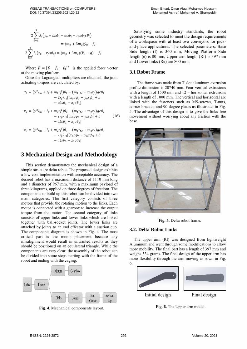
profile dimension is 20*40 mm. Four vertical extrusions with a length of 1500 mm and 12 – horizontal extrusions with a length of 1000 mm. The vertical and horizontal are linked with the fasteners such as M5-screws, T-nuts, corner bracket, and 90-degree plates as illustrated in Fig. 5. The advantage of this design is to give the links free movement without worrying about any friction with the base.

Fig. 5. Delta robot frame.

3.2. Delta Robot Links

The upper arm (Rf) was designed from lightweight Aluminum and went through some modifications to allow more mobility. The final part has a length of 397 mm and weighs 534 grams. The final design of the upper arm has more flexibility through the arm moving as sown in Fig. 6.

Fig. 6. The Upper arm model.

Initial design Final design



E-ISSN: 2224-2872 292 Volume 20, 2021

The upper arm loads the lower links with payload which are estimated at 41 N. Moreover, the motor torque can be determined with 3 N.m. After applying the previous loads on the upper arm, the displacement analysis of the upper arm is an acceptable range and safe as demonstrated in Fig. 7.

Fig. 7. Displacement analysis of the upper link.

The upper-link is formed by laser cutting for an aluminium sheet with 8mm thickness. After cleaning the link, it will be connected to the motor with a flange shown in Fig. 8.

Fig. 8. Flange connector for the upper link.

The steps of manufacturing and implementation of the upper link are illustrated in Fig. 9. The first step uses the aluminum sheet as a raw material to laser cut machine. The required form will be obtained after the machining. In the next step, the obtained upper arm needs to surface finish. The last step is connecting the flange to the upper arm.

Fig. 9. Manufacturing & Implementation of the upper

link.

The lower links are formed using 8mm diameter stainless steel rods. The manufacturing of the links made by a turning machine to reduce the length from 1000mm to 764mm and to thread the ends of the rod by 25mm long and diameter 5mm. While the manufacturing is completed, the upper link will be

connected with the ball-socket joint (Fig. 10) by spacer and screw as shown in Fig. 11. The lower link then will be attached with the joint by the threading. The steps are in Fig. 12.

Fig. 10. Ball-socket joint.

Fig. 11. Connecting joint with the upper link.

Fig. 12. Manufacturing & Implementation of the lower link.

3.3. End Effector of Delta Robot The components of the end effector as shown in Fig.

13 are formed with laser cutting for an aluminum sheet with 8mm thickness, a suction cup for grasping the object, and a flange to connect them. it will be connected to the lower link with the joint, and with the suction cup with the flange.

Fig. 13. End-effector components.



E-ISSN: 2224-2872 293 Volume 20, 2021

The procedure of implementing the end-effector is illustrated in Fig. 14. After connecting the end effector.

Fig. 14. Manufacturing & Implementation of the end-

effector.

3.4. Suction Gripper

Vacuum/suction cups grip a workpiece by evacuating air from the space inside the cup, creating a partial vacuum at a pressure below ambient. In simple terms, one can size a vacuum cup based on the load, available vacuum, and cup area. The theoretical suction force is the cup force acting perpendicular to the workpiece surface. Theoretical holding force (𝐹𝑡) is simply:

𝐹𝑡 = ΔP × A (17)

Where ΔP is the difference between ambient and system pressure and A acts the effective area of the suction cup under vacuum. But in the actual holding force, there are several other factors that should be considered. The first factor is the safety factor where calculations should include a safety factor due to many external influences affect actual performance. The value of the safety factor is at least 1.5.

Many vacuum-system manufacturers recommend a safety factor of at least 2.0. In high-speed swinging or swiveling operations, the safety of 2.5 or higher might be needed to ensure a tight grip on work pieces and the safety of nearby workers. The second factor are Load, orientation, and acceleration forces. The diameter should be calculated and the effective gripping area of a vacuum cup. So, it is preferred to determine the necessary holding force. range of cups can be chosen that meet the requirements based on size, shape, material, cost, and manufacturer.

For a horizontal vacuum cup with a vertical lifting force as shown in Fig. 15.

Fig. 15. Schematic for vacuum cup lifting force.

The following table 1 and Fig. 16 show the relationship between nozzle diameter and the pressure pump to optimize these parameters with each other. The suitable pump at maximum payload (mp=3Kg) has a minimum pressure of 118 KPa and a nozzle diameter of 27 mm.

Table 1. Relation between nozzle diameter and the pressure pump at mp=3Kg.

Fig. 16. Relation between nozzle diameter and the

pressure pump at m=3Kg and F=67.5N.

D(mm) P(KPa) D(mm) P(KPa)

5 3438 13 509

6 2387 14 438

7 1754 15 382 8 1343 16 336

9 1061 17 297

10 859 18 265

11 710 19 238

12 597 20 215

0

500

1000

1500

2000

2500

3000

3500

4000

5 6 7 8 9 1011121314151617181920

Pre

ssu

re(K

Pa)

Diameter (mm)



E-ISSN: 2224-2872 294 Volume 20, 2021

3.5. Robot Assembly

The mechanical components of the delta robot will be assembled as demonstrated in Fig. 17. The geared stepper motor is coupled with the upper arms which are connected with lower links. finally, the lower links are gathered with the end effector at one point.

Fig. 17. Final assembly of the delta robot.

4 Electrical Design and Control This section illustrates the actuator sizing steps of the

delta robot. Also, it displays the control algorithm and camera object detection. Moreover, it demonstrates the required pressure of the suction cup gripper. 4.1. Actuator Sizing and Control

This subsection determines the required torque of the

delta robot through the movement to execute the tasks with the desired speed and acceptable accuracy. It is known that stepper motors move in discrete steps of a revolution. For example, a stepper motor with a 1.8-degree step angle will make 200 steps for every full revolution of the motor (360÷1.8=200). This discrete motion means the motor’s rotation is not perfectly smooth, due to the relatively large step size. One way to improve the resolution and the movement is smooth is to reduce the size of the motor’s step, this is known as the micro-stepping process.

Micro-stepping control divides each full step into smaller steps to improve the resolution and the movement smoothly. For example, a 1.8-degree step can be divided up to 256 times, providing a step angle of 0.007 degrees (1.8 ÷ 256).

Micro stepping is achieved by using pulse-width modulation (PWM) voltage to control the current to the motor windings. The driver sends two voltage sine waves, 90 degrees out of phase, to the motor windings. While current increases in one winding, it decreases in the other winding. This achieves smoother motion than full or half-step control.

Table 2 shows the relation between the micro-step and

the torque output from the motor.

Table 2. The relation between micro step & torque.

Micro step/ Full Step % Torque/ Micro step

1 100% 2 70.71% 4 38.27% 8 19.51%

16 9.8% 32 4.91% 64 2.45%

128 1.23% 256 0.61%

The required torque motors equations were

demonstrated in equation (16). So, by substituting in delta robot designed parameters as shown in table 2. From equation (16) and the delta robot system parameters in table 3 can obtain the required torque (𝝉1 = 3.07 Nm, 𝝉2 = 2 Nm, and 𝝉3 =2.94 Nm). A gearbox has a reducer factor ratio of 5:1 to increase the torque output. So, the suitable motor torque is 8 Nm with micro-step (16). Where, 8 × (9.8 ÷ 100) × 5 = 3.92 Nm. Table 3. Parameters and their values of the torque equations (16).

Parameter Value Parameter value

𝜆 1 -15.1458 𝑟𝑓 366 mm 𝜆 2 -13.238 𝑟𝑓𝑐 183 mm 𝜆 3 -16.4696 𝛾 5:1 �̈�1 15.02 rad/s2 𝐼𝑚 0.5x10-4

kgm2 �̈�2 12.02 rad/s2 𝐼1 80x10-4

kgm2 �̈�3 17.36 rad/s2 m1 200 g g 9.81 m/s2 m2 400 g

X0 70.45 mm mp 200 g Y0 -116.6 mm a 370 mm Z0 -819 mm b 40 mm 𝜃1 15o 𝜙1 60o 𝜃2 25o 𝜙2 180o 𝜃3 35o 𝜙3 -60o

The technical specifications of the required stepper

motor are shown in table 4.



E-ISSN: 2224-2872 295 Volume 20, 2021

Table 4. Stepper motor NEMA 34 parameters

Step Angle 1.8°

Current /phase 4.2 A

Inductance /phase 6 mH

Holding Torque 85 Kg.cm = 8.3 Nm

leads 8 wires

Motor Wight 3.8 Kg

Length 118 mm

As mentioned in the previous section, the mechanism

requires using NEMA 34 Stepper motor, taking advantage of micro-stepping to achieve higher angular motion resolution, at the cost of decreasing the operating torque. The micro-stepping condition can achieve using an EM882S driver which is capable of powering and controlling 2-phase and 4-phase stepper motors with a smooth motion with low motor (stator) heating and noise. It requires a supply voltage range from 20-80 VDC and outputs from 0.5 to 8.2 Amps. It supports the Step-and-direction control type with smooth filtering that can be tuned and configured using the manufacturer software (Leadshine ProTuner). The Driver Pin Configuration is shown in Fig. 18.

Fig. 18. Stepper Drive.

There are two methods that can be used to achieve closed-loop control. In the first method, the PID controller will be programmed in the microcontroller (Arduino) and the driver works as an amplifier of the input signal as demonstrated in Fig. 19. The second method, the PID controller is built in the motor driver (using the auto-tuning option) as illustrated in Fig. 20. The setpoint is calculated using the inverse kinematics algorithm.

Fig. 19. The first method of the closed-loop delta robot

system.

Fig. 20. The second method of the closed-loop delta

robot system.

Fig. 21 demonstrates the flow chart of the delta robot control algorithm using Arduino mega microcontroller. In the beginning, the camera detects the product through the scanning area and determines the coordinates of the product. The next step, applying inverse kinematics equations to estimate the set points of the stepper motor. After that, the controller algorithm determines the path planning from delta robot home positioning to the initial position of the product (the first path) and from the initial position to the final destination of the product (the second path). The gripper will be activated to catch the product and translate it to the final destination.

Fig. 21. The flow chart of the delta robot control

algorithm.



E-ISSN: 2224-2872 296 Volume 20, 2021

4.2. Pixy2 Camera Contrary to the complexity in the mechanical design,

the robot needs to can complete the inverse kinematics and trajectory control tasks. The most important sensor element is the camera as demonstrated in Fig. 22. The Pixy 2 Camera was used to provide sensory feedback in the form of vision. This type of this camera can distinguish the color of the object but cannot estimate the object Topology as shown in Fig. 23. This camera can determine the coordinate of delta robot end effector. So, it is possible to estimate the angles of links using inverse kinematics calculations.

Fig. 22. Pixy2 Camera.

Fig. 23. Operating modes: Color Detection – Line Tracking.

5 Delta Robot Performance and

Specifications After the assembly of both mechanical and electrical

systems of the Delta Robot, it has been ready for testing to ensure the functionality and the reliability of each system and the robot as a complete unit. In this section, the results acquired are written alongside the safety procedures during maintenance and operation. This section also includes the robot specifications, advantages, and limitations. There are several tests done on each system of the Delta Robot to check its functionality with acceptable performance.

5.1. Camera Unit Tests In the camera unit, two tests were done to aiming to achieve to receive steady responses and ensure its function works reliably. In the first test, the camera is mounted at the same origin as the robot's global origin, then the camera setup software is opened to set the object color signatures. This test resulted in occlusion by the robot linages as shown in Fig. 24.

Fig. 24. Camera Output with Linkages Occlusion.

In the second test, To get a clear image without any occlusion, the robot linkages are moved to a specific preset position to clear any obstacles from the camera field of vision as shown in Fig. 25 and Fig. 26. After this test we achieved stable object coordinates, ready to be calibrated and adjusted to the robot coordinates.

Fig. 25. Camera vision without occlusion.



E-ISSN: 2224-2872 297 Volume 20, 2021

Fig. 26. Preset position of Robot links.

After the second test, the camera coordinates system

is manipulated through transformation equations to get the corresponding coordinates on the robot global coordinate system as shown in Fig. 27.

Fig. 27. Final Coordinates after Calibration.

5.2. Pneumatic Suction Unit Tests

Two tests were implemented to validate the maximum holding force of the suction cup at an operating nominal air pressure of 5 bar, which results in a negative pressure of 80 Kpa through the vacuum generator. The purpose of the first test is to make sure that the pneumatic circuit (presented in the previous section) is functioning reliably with the required holding torque as shown in Fig. 28.

Fig. 28. Suction Demo for Holding Force of 3 Kg.

The objective of the second test is to validate the functionality after mounting the suction cup on the end effector platform, as shown in Fig. 29, thus ensuring the rigidity of the mechanism after holding the rated payload. The pneumatic suction cup end effector was capable of providing a holding force of at least 3 Kg with a cup diameter of 50 mm at a nominal air pressure of 4 Bar.

Fig. 29. Holding while mounted on the robot.

5.3. Motors and Drivers Unit Tests In this section, the motor and drive system of the delta

robot will be validated to ensure that the end effector can execute the inverse kinematics commands to track a preselected path based on camera position reading. Several tests were developed to check the motor's max operating speed, acceleration, and positioning.

The first test examines the relationship between the pulses frequency and the motor speed. Through the test, the motor speed increases gradually with increasing the frequency of pulses.



E-ISSN: 2224-2872 298 Volume 20, 2021

Also, the robot vibration was in an acceptable range which did not affect the required tasks of the robot. The second test validates the three velocity profiles that were used: rectangular, trapezoidal, and S-Curve profile. The rectangular creates huge vibrations due to rapid change in acceleration. Although the S-curve (Fig. 30) is ideal, it was difficult to implement to change the frequencies of the pulse accordingly. The Trapezoidal profile was easier to use and resulted in minimal vibration.

Fig. 30. Simplified S-Curve Velocity Profile.

During this test, the gearbox was connected to the motors alongside the encoders to validate the positioning accuracy, considering the gear ratio. The motors can move with a velocity of 30 degrees per second with a trapezoidal velocity profile with 1/3 acceleration, 1/3 run velocity, and 1/3 deceleration. Moreover, the robot was able to accelerate and hold its position at the rated payload of 3 Kg. The actual positioning accuracy was computed by the built-in encoders with an accuracy of 0.09o deviation from the set point on the motor shaft and equals 0.018o on the gearbox output shaft.

The specifications of the Industrial Delta Robot

(IDR) are shown in Table 6.

Table 6. Delta Robot Specifications

Payload 3 Kg

Workspace (LxWxH) 560x560x300mm3

Accuracy ± 0.85 mm

Repeatability ± 1.5 mm

Velocity 0.5 m/s Acceleration 2 m/s2

It can be noted that the velocity and the acceleration can be higher but requires a stiffer base and an enhanced velocity profile.

6 Conclusion

An efficient with low-cost delta robot was designed

and implemented where the main functions of pick and place applications can be used to automate a production line with a workspace of 560x560x300 cubic millimeters with a maximum payload of 3 kg. Equipped with a camera to provide computer vision, using Pixy2 Cam. The main actuators used are NEMA-34 closed-loop stepper motors to achieve high positioning accuracy. The suction mechanism of the end effector is performed using a pneumatic vacuum generator alongside its supplementary components. In the end, the robot was designed, implemented, and tested. The robot was manufactured with the minimum possible cost of 34,000 EGP that achieve a high level of reliability. The robot operation cycle was tested, and problems were solved as much as possible to reach an appropriate performance.

Acknowledgements

I want to thank Eng. Shaima Zidan for her efforts through this project. References:

[1] K. Rosquist, “Modelling and Control of a Parallel

Kinematic Robot,” p. 65, 2013.

[2] S. B. Park, H. S. Kim, C. Song, and K. Kim, “Dynamics

modeling of a Delta-type parallel robot (ISR 2013),”

Yonsei University, 2013.

[3] A. J. Humaidi, A. I. Abdulkareem, and W. Zhang, “Design

of augmented nonlinear PD controller of Delta/Par4-like

robot,” J. Control Sci. Eng., vol. 2019, 2019, doi:

10.1155/2019/7689673.

[4] K. Miller, “Experimental verification of modeling of

DELTA robot dynamics by direct application of Hamilton’s

principle,” Proc. - IEEE Int. Conf. Robot. Autom., vol. 1,

pp. 532–537, 1995, doi: 10.1109/ROBOT.1995.525338.

[5] Q. Zhao, P. Wang, and J. Mei, “Controller parameter

tuning of delta robot based on servo identification,”

Chinese J. Mech. Eng. (English Ed., vol. 28, no. 2, pp.

267–275, 2015, doi: 10.3901/CJME.2014.1117.169.

[6] A. Codourey, “Dynamic Modeling of Parallel Robots for

Computed-Torque Control Implementation,” Int. J. Rob.

Res., vol. 17, no. 12, pp. 1325–1336, 1998, doi:

10.1177/027836499801701205.

[7] D. Kato, K. Yoshitsugu, T. Hirogaki, E. Aoyama, and K.

Takahashi, “Predicting positioning error and finding

features for large industrial robots based on deep

learning,” Int. J. Autom. Technol., vol. 15, no. 2, pp. 206–

214, 2021, doi: 10.20965/IJAT.2021.P0206.

[8] L. Angel and J. Viola, “Fractional order PID for tracking

control of a parallel robotic manipulator type delta,” ISA

Trans., vol. 79, no. May, pp. 172–188, 2018, doi:

10.1016/j.isatra.2018.04.010.

[9] Z. Sabir, M. A. Z. Raja, D.-N. Le, and A. A. Aly, “A neuro-

swarming intelligent heuristic for second-order nonlinear

Lane–Emden multi-pantograph delay differential system,”



E-ISSN: 2224-2872 299 Volume 20, 2021

Complex Intell. Syst., no. 0123456789, 2021, doi:

10.1007/s40747-021-00389-8.

[10] F. C. Can, M. Hepeyiler, and Ö. Başer, “A Novel Inverse

Kinematic Approach for Delta Parallel Robot,” Int. J.

Mater. Mech. Manuf., vol. 6, no. 5, pp. 321–326, 2018,

doi: 10.18178/ijmmm.2018.6.5.400.

[11] Y. L. Kuo, “Mathematical modeling and analysis of the

Delta robot with flexible links,” Comput. Math. with Appl.,

vol. 71, no. 10, pp. 1973–1989, 2016, doi:

10.1016/j.camwa.2016.03.018.

[12] M. H. Falsafi, K. Alipour, and B. Tarvirdizadeh, “Fuzzy

motion control for wheeled mobile robots in real-time,” J.

Comput. Appl. Res. Mech. Eng., vol. 8, no. 2, pp. 133–144,

2019, doi: 10.22061/jcarme.2018.2204.1205.

[13] M. A. Shamseldin, M. Sallam, A. M. Bassiuny, and A. M.

Abdel Ghany, “LabVIEW implementation of an enhanced

nonlinear PID controller based on harmony search for

one-stage servomechanism system,” J. Comput. Appl. Res.

Mech. Eng., vol. 12, pp. 4161–4179, 2019, doi:

10.15282/jmes.12.4.2018.13.0359.

[14] M. A. Shamseldin, M. Sallam, A. M. Bassiuny, and A. M.

A. Ghany, “A new model reference self-tuning fractional

order PD control for one stage servomechanism system,”

WSEAS Trans. Syst. Control, vol. 14, pp. 8–18, 2019.

[15] M. A. Shamseldin, “Optimal Coronavirus Optimization

Algorithm Based PID Controller for High Performance

Brushless DC Motor,” 2021.

[16] W. P. Feng, Z. L. Min, and Z. X. Man, “Dynamic

modeling, simulation and experiment of the delta robot,”

Lect. Notes Electr. Eng., vol. 141 LNEE, no. VOL. 1, pp.

149–156, 2012, doi: 10.1007/978-3-642-27311-7_20.

[17] C. Gallacher, J. Willes, and J. Kovecses, “Parasitic effects

of device coupling on haptic performance,” IEEE World

Haptics Conf. WHC 2015, no. November, pp. 266–272,

2015, doi: 10.1109/WHC.2015.7177724.

[18] S. Makita, T. Sasaki, and T. Urakawa, “Offline direct

teaching for a robotic manipulator in the computational

space,” Int. J. Autom. Technol., vol. 15, no. 2, pp. 197–

205, 2021, doi: 10.20965/IJAT.2021.P0197.

[19] S. A. Bortoff, “Object-Oriented Modeling and Control of

Delta Robots,” 2018 IEEE Conf. Control Technol. Appl.

CCTA 2018, no. August 2018, pp. 251–258, 2018, doi:

10.1109/CCTA.2018.8511395.

[20] M. Rachedi, “Model based control of 3 DOF parallel

delta robot using inverse dynamic model,” 2017 IEEE Int.

Conf. Mechatronics Autom. ICMA 2017, pp. 203–208,

2017, doi: 10.1109/ICMA.2017.8015814.

Creative Commons Attribution License 4.0 (Attribution 4.0 International, CC BY 4.0)

This article is published under the terms of the Creative Commons Attribution License 4.0 https://creativecommons.org/licenses/by/4.0/deed.en_US



E-ISSN: 2224-2872 300 Volume 20, 2021

Design and Implementation of a Low-Cost Microcontroller ...

Documents

Transcript of Design and Implementation of a Low-Cost Microcontroller ...