Design and experimental validation of a new bandwidth ... · The main idea is to prioritize...
100
Politecnico di Milano School of Industrial and Information Engineering Master of Science in Telecommunication Engineering Electronics, Information and Bioengineering Department Design and experimental validation of a new bandwidth sharing scheme based on dynamic queue assignment Supervisor: Prof. Antonio Capone Supervisor: Prof. Brunilde Sans` o Advisor: Eng. Carmelo Cascone Graduation Thesis of: Luca Bianchi Student ID 817219 Academic Year 2015-2016
Transcript of Design and experimental validation of a new bandwidth ... · The main idea is to prioritize...
Politecnico di MilanoSchool of Industrial and Information Engineering
Master of Science in Telecommunication EngineeringElectronics, Information and Bioengineering Department
2.2 . | il marchio, il logotipo: le declinaZioni
Design and experimental validation
of a new bandwidth sharing scheme
based on dynamic queue assignment
Supervisor: Prof. Antonio CaponeSupervisor: Prof. Brunilde SansoAdvisor: Eng. Carmelo Cascone
Graduation Thesis of:Luca Bianchi
Student ID 817219
Academic Year 2015-2016


Acknowledgements
First of all I would like to express my gratitude to my supervisors, Prof. Capone
and Prof. Sanso, for giving me the incredible opportunity to live a long and intense
experience abroad. Many thanks to Prof. Capone for the illuminating advices and
for following the project with passion.
Many thanks to Prof. Sanso for the numerous and precious advices in all areas,
for providing us all the spaces and devices to run tests and for correcting with
great care the thesis.
A special thanks to Carmelo, for the opportunity to work on such an interesting
project, for being a charismatic leader and example to me, for pushing me in the
right direction when I was loosing the focus and for giving me a lot of precise
technical advices and programming lessons.
I would like to thank Luca, for all the office talks that allowed me to face
problems from different points of view and for all the coffee breaks that helped to
carry on during the long working days.
Thanks to the GERAD’s technical staff for the help in the set up and mainte-
nance of the testbed and for not getting upset after the ”network benchmarking”
incident.
Finally, I would like to thank my parents for the encouragement and the sup-
port they gave me during all the academic career.
3


Contents
1 Introduction 15
1.1 Context . . . . . . . . . . . . . . . . . . . . . . . . . . . . . . . . 15
1.2 Objective . . . . . . . . . . . . . . . . . . . . . . . . . . . . . . . 16
1.3 Problem statement . . . . . . . . . . . . . . . . . . . . . . . . . . 17
1.4 Summary . . . . . . . . . . . . . . . . . . . . . . . . . . . . . . . 18
2 State of the art 19
2.1 End-to-end congestion control . . . . . . . . . . . . . . . . . . . . 20
2.2 Scheduling . . . . . . . . . . . . . . . . . . . . . . . . . . . . . . . 21
2.3 Active Queue Management . . . . . . . . . . . . . . . . . . . . . . 24
2.4 Dynamic assignment of queues . . . . . . . . . . . . . . . . . . . . 27
2.5 Analysis . . . . . . . . . . . . . . . . . . . . . . . . . . . . . . . . 28
3 Approach 30
3.1 Main idea . . . . . . . . . . . . . . . . . . . . . . . . . . . . . . . 30
3.1.1 UGUALE with two queues . . . . . . . . . . . . . . . . . . 31
3.1.2 UGUALE with more queues . . . . . . . . . . . . . . . . . 32
3.2 Pipeline . . . . . . . . . . . . . . . . . . . . . . . . . . . . . . . . 34
3.2.1 Flow Aggregation . . . . . . . . . . . . . . . . . . . . . . . 34
3.2.2 Metering . . . . . . . . . . . . . . . . . . . . . . . . . . . . 36
3.2.3 Classification . . . . . . . . . . . . . . . . . . . . . . . . . 36
3.2.4 Scheduling . . . . . . . . . . . . . . . . . . . . . . . . . . . 37
5
CONTENTS
3.3 Thresholds setting . . . . . . . . . . . . . . . . . . . . . . . . . . 37
3.3.1 First threshold . . . . . . . . . . . . . . . . . . . . . . . . 37
3.3.2 Other thresholds . . . . . . . . . . . . . . . . . . . . . . . 37
3.4 Enhancements . . . . . . . . . . . . . . . . . . . . . . . . . . . . . 40
3.4.1 Ad hoc thresholds . . . . . . . . . . . . . . . . . . . . . . . 40
3.4.2 Maximum Marking Rate . . . . . . . . . . . . . . . . . . . 41
3.4.3 Round Trip Time compensation . . . . . . . . . . . . . . . 42
4 Implementation 47
4.1 Testbed . . . . . . . . . . . . . . . . . . . . . . . . . . . . . . . . 47
4.2 Switch . . . . . . . . . . . . . . . . . . . . . . . . . . . . . . . . . 49
4.3 Pipeline . . . . . . . . . . . . . . . . . . . . . . . . . . . . . . . . 51
4.4 Strict Priority scheduler . . . . . . . . . . . . . . . . . . . . . . . 53
4.5 Meters . . . . . . . . . . . . . . . . . . . . . . . . . . . . . . . . . 55
4.5.1 Series of token bucket filters meter . . . . . . . . . . . . . 56
4.5.2 Iptables estimator meter . . . . . . . . . . . . . . . . . . . 58
4.6 Collecting data . . . . . . . . . . . . . . . . . . . . . . . . . . . . 60
4.7 Emulating more users . . . . . . . . . . . . . . . . . . . . . . . . . 62
4.7.1 Emulating users with different Round Trip Times . . . . . 64
5 Experimental results 68
5.1 Test . . . . . . . . . . . . . . . . . . . . . . . . . . . . . . . . . . 68
5.1.1 Test validation . . . . . . . . . . . . . . . . . . . . . . . . 69
5.1.2 Data analysis . . . . . . . . . . . . . . . . . . . . . . . . . 70
5.1.3 Data presentation . . . . . . . . . . . . . . . . . . . . . . . 71
5.1.4 Test configuration . . . . . . . . . . . . . . . . . . . . . . . 73
5.1.5 Outline of tests . . . . . . . . . . . . . . . . . . . . . . . . 74
5.2 Results . . . . . . . . . . . . . . . . . . . . . . . . . . . . . . . . . 75
5.2.1 Switch in standalone fail-mode . . . . . . . . . . . . . . . . 75
6

CONTENTS
5.2.2 UGUALE . . . . . . . . . . . . . . . . . . . . . . . . . . . 79
5.2.3 UGUALE with ad hoc thresholds . . . . . . . . . . . . . . 83
5.2.4 UGUALE with MMR . . . . . . . . . . . . . . . . . . . . . 85
5.2.5 UGUALE with RTT compensation . . . . . . . . . . . . . 87
5.2.6 Type of meter . . . . . . . . . . . . . . . . . . . . . . . . . 88
5.3 Length of switch queues . . . . . . . . . . . . . . . . . . . . . . . 90
6 Conclusion 92
6.1 Future works . . . . . . . . . . . . . . . . . . . . . . . . . . . . . 93
7

List of Figures
2.1 Example of hierarchical scheduler . . . . . . . . . . . . . . . . . . 22
3.1 Example of the UGUALE scheme with 2 bands . . . . . . . . . . 32
3.2 Example of the UGUALE scheme with 4 bands . . . . . . . . . . 33
3.3 UGUALE’s pipeline . . . . . . . . . . . . . . . . . . . . . . . . . . 34
3.4 UGUALE’s detailed pipeline . . . . . . . . . . . . . . . . . . . . . 35
3.5 Unfair assignment of bands . . . . . . . . . . . . . . . . . . . . . . 38
3.6 Fair assignment of bands . . . . . . . . . . . . . . . . . . . . . . . 39
3.7 Ad hoc assignment of bands . . . . . . . . . . . . . . . . . . . . . 40
3.8 Symmetric assignment of bands . . . . . . . . . . . . . . . . . . . 41
3.9 Assignment of bands with the Maximum Marking Rate strategy . 43
3.10 Rate dependence from the RTT . . . . . . . . . . . . . . . . . . . 44
3.11 Multiplier to compensate the rate dependence from the RTT . . . 45
3.12 Adjusted multiplier for the RTT compensation method . . . . . . 46
4.1 Photo of the testbed . . . . . . . . . . . . . . . . . . . . . . . . . 48
4.2 Scheme of the testbed . . . . . . . . . . . . . . . . . . . . . . . . 49
4.3 UGUALE’s pipeline with an OpenFlow switch . . . . . . . . . . . 52
4.4 UGUALE’s adapted pipeline . . . . . . . . . . . . . . . . . . . . . 52
4.5 Process to obtain a SP scheduler . . . . . . . . . . . . . . . . . . 54
4.6 Token bucket scheme . . . . . . . . . . . . . . . . . . . . . . . . . 55
4.7 OpenFlow meter . . . . . . . . . . . . . . . . . . . . . . . . . . . 56
4.8 Meter implemented with a series of token bucket filters . . . . . . 57
8

LIST OF FIGURES
4.9 Output of different types of meter . . . . . . . . . . . . . . . . . . 58
4.10 Meter implemented with iptables . . . . . . . . . . . . . . . . . . 59
4.11 Screenshot of plotServer . . . . . . . . . . . . . . . . . . . . . . . 61
4.12 Screenshot of plotServer . . . . . . . . . . . . . . . . . . . . . . . 62
4.13 Testbed configured to emulate many users . . . . . . . . . . . . . 63
4.14 PC configuration to emulate many users with different delays . . . 67
5.1 Test file structure . . . . . . . . . . . . . . . . . . . . . . . . . . . 69
5.2 Baseline test with OVS standalone . . . . . . . . . . . . . . . . . 76
5.3 Different TCP connections with OVS standalone . . . . . . . . . . 77
5.4 Different RTTs with OVS standalone . . . . . . . . . . . . . . . . 78
5.5 Different connections with UGUALE . . . . . . . . . . . . . . . . 79
5.6 Different RTTs with UGUALE . . . . . . . . . . . . . . . . . . . 80
5.7 Band assignment to study the fairness dependence from the width
of bands. . . . . . . . . . . . . . . . . . . . . . . . . . . . . . . . . 81
5.8 Fairness dependence from the width of bands . . . . . . . . . . . . 82
5.9 Result for the ad hoc thresholds assignment . . . . . . . . . . . . 84
5.10 Different TCP connections with UGUALE and the MMR . . . . . 85
5.11 Different RTTs with UGUALE and the MMR . . . . . . . . . . . 86
5.12 UGUALE with RTT comprensation . . . . . . . . . . . . . . . . . 87
5.13 RTT compensation statistics . . . . . . . . . . . . . . . . . . . . . 88
5.14 Different number of TCP connections with UGUALE and token
bucket meters . . . . . . . . . . . . . . . . . . . . . . . . . . . . . 89
5.15 Different RTTs with OVS standalone and long queues . . . . . . . 91
9
List of Tables
3.1 Example of aggregation table . . . . . . . . . . . . . . . . . . . . 35
5.1 Statistics of different meter implementations . . . . . . . . . . . . 89
10


Abstract
Even if the fair sharing of available resources in the network has been oneof the basic principles since the Internet beginnings, it is still today notfully implemented. The fairness among traffic flows is mainly managed bythe transport layer and the network does not have an active role but it justprovides a Best Effort type of service without quality guarantees.
The objective of the work is to present a practical solution to thebandwidth sharing problem in a network node. Therefore, the current ap-proaches were analyzed in order to propose an original and ready for usescheme. The new bandwidth sharing allocation engine (named UGUALE)works by assigning packets to the queues of a Strict Priority scheduler basedon the measured rate offered by users.
The main idea is to prioritize well-behaving users in order to collaboratewith the end-to-end congestion control mechanisms they implement at thetransport or application layer. The allocation engine was implemented withthe abstractions made available by the OpenFlow switch model and APIs,with the aim of proposing a solution amenable to be deployed in existingSoftware Defined Networking (SDN) architectures. Moreover, UGUALE iseasy to configure since the only requested parameters are the guaranteedrates that users should obtain.
To validate our approach, a real testbed composed of five PCs was set upand several automation and monitoring scripts were written. When tested,the proposed allocation engine proved to be very effective in guaranteeingminimum rates and in the fair allocation of the free capacity, even whenusers have a different number of TCP connections or different Round TripTimes (RTTs). In conclusion, the promising results obtained by UGUALEmakes us believe that such an approach is worth of further analysis.
12

Sommario
Sebbene l’equa condivisione delle risorse di rete sia stata uno dei principifondamentali sin dagli inizi di Internet, ad oggi non e ancora stata comple-tamente implementata. La ripartizione della banda tra i flussi di traffico egestita principalmente dal livello di trasporto, pertanto la rete non ha unruolo attivo ma fornisce semplicemente un tipo di servizio Best Effort senzagaranzie di qualita.
L’obiettivo del lavoro e di presentare una soluzione pratica al problemadella suddivisione della banda in un nodo della rete. Per questo motivoabbiamo analizzato le soluzioni attuali cosı da poter proporre uno schemainnovativo e di facile adozione. Il nuovo schema di allocazione di banda(chiamato UGUALE) e basato sull’assegnamento dei pacchetti alle code diuno scheduler Strict Priority in base al tasso d’arrivo offerto dagli utenti.
L’idea si basa sulla prioritizzazione degli utenti che rispettano i proprilimiti cosı da collaborare con i meccanismi di controllo di congestione im-plementati al livello di trasporto o applicativo. Lo schema di allocazione estato implementato con le astrazioni rese disponibili dal modello di switchOpenFlow e dalle sue API, con lo scopo di proporre una soluzione facil-mente utilizzabile nelle architetture Software Defined Networking (SDN)gia esistenti. UGUALE e facile da configurare siccome l’unico parametrorichiesto e la banda da garantire a ciascun utente.
Al fine di verificare la bonta della nostra soluzione, abbiamo configuratouna rete composta da cinque computer, inoltre abbiamo scritto diversi pro-grammi per automatizzare i test e per controllare in tempo reale la suddivi-sione della banda. Dai test emerge che UGUALE e efficace nel garantire labanda minima e nell’allocare equamente la banda eccedente, anche quandogli utenti hanno un numero diverso di connessioni TCP o dei Round TripTime (RTT) differenti. In conclusione, visti i risultati promettenti ottenuti,siamo convinti che il funzionamento dello schema di allocazione propostomeriti ulteriori approfondimenti.
13


Chapter 1
Introduction
1.1 Context
Today’s Internet is still facing the problem of congestion control, due to the in-
creasing number of users and the convergence of many services on the global
network. The architecture of the Internet is still too much Best Effort oriented, in
the sense that routers rarely implement technologies to guarantee fairness between
users and to maximize the network utilization at the same time. In the most com-
mon case users’ flows share the same link served with a First In First Out (FIFO)
queue, loosing any chance to apply fairness schemes able to guarantee a certain
rate to every one. In fact connections that do not implement any end-to-end con-
gestion control mechanism might end up monopolizing queues, finally preventing
other users to access the link capacity. Most Internet traffic is TCP-compatible [2]
but the end-to-end congestion control mechanisms apply only to separate flows.
This means that a user can obtain more bandwidth by instantiating many con-
nections to the same destination, thus violating the intrinsic TCP fairness at the
user level. Hence end-to-end mechanisms are not enough to guarantee per-user
fairness because they are not collaborative. Nevertheless telecommunication op-
erators need to sell services on a per-user basis, for example charging more users
who desire high bandwidth and low delay. Operators tend to solve the bandwidth
sharing problem implementing different solutions that perform good enough only
15

CHAPTER 1. INTRODUCTION
if combined with over-provisioned networks. Summarizing, the standard schemes
produce a coarse per-user fairness, oblige operators to stipulate contracts based
on the maximum rate achievable by users and result in a low network efficiency
from the point of view of the link utilization.
1.2 Objective
For the reason sustained in [5], we agree that fairness should be guaranteed and
enforced between users and not between connection layer flows. A user is defined
as an arbitrary aggregate of connection layer flows.
The objective of this work is to propose, implement and analyze a new for-
warding engine able to guarantee a weighted fairness between users in a network
node. The system, to be applied on real network switches, should produce some
features like:
Scalability The ability to operate with a large number of users.
Flexibility The parameters of the system must be easily modifiable.
Stability The system should produce a stable output, so that rate oscillations
are contained.
Performance The system should be able to manage an high total transmission
rate.
Efficiency In presence of elastic traffic the aggregate throughput must be always
the maximum allowed by the link.
16
CHAPTER 1. INTRODUCTION
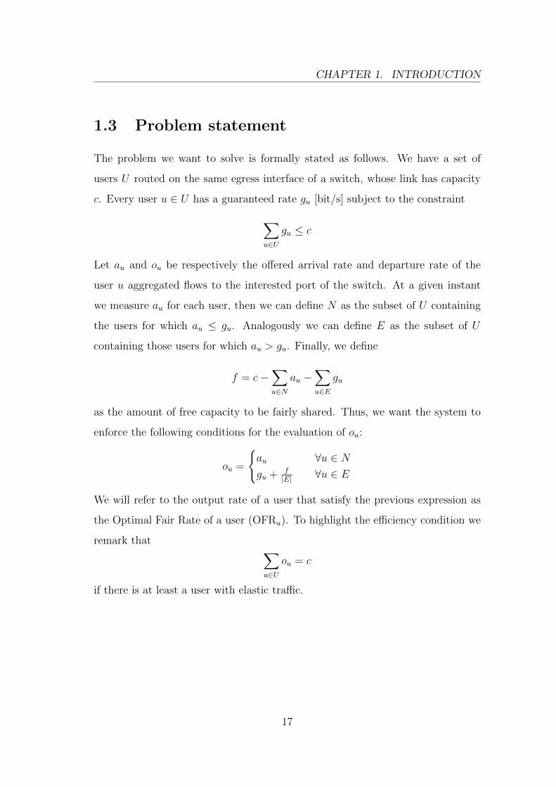
1.3 Problem statement
The problem we want to solve is formally stated as follows. We have a set of
users U routed on the same egress interface of a switch, whose link has capacity
c. Every user u ∈ U has a guaranteed rate gu [bit/s] subject to the constraint∑u∈U
gu ≤ c
Let au and ou be respectively the offered arrival rate and departure rate of the
user u aggregated flows to the interested port of the switch. At a given instant
we measure au for each user, then we can define N as the subset of U containing
the users for which au ≤ gu. Analogously we can define E as the subset of U
containing those users for which au > gu. Finally, we define
f = c−∑u∈N
au −∑u∈E
gu
as the amount of free capacity to be fairly shared. Thus, we want the system to
enforce the following conditions for the evaluation of ou:
ou =
{au ∀u ∈ N
gu + f|E| ∀u ∈ E
We will refer to the output rate of a user that satisfy the previous expression as
the Optimal Fair Rate of a user (OFRu). To highlight the efficiency condition we
remark that ∑u∈U
ou = c
if there is at least a user with elastic traffic.
17

CHAPTER 1. INTRODUCTION
1.4 Summary
The bandwidth sharing problem defined in section 1.3 is faced in the rest of
the document that is organized as follows. In chapter 2 the current standard
solutions to bandwidth sharing are analyzed to understand their main drawbacks.
In chapter 3 our approach to the problem is proposed and described in detail.
In chapter 4 the implementation of the proposed scheme on a real testbed is
illustrated, taking into considerations all the practical problems encountered and
the solutions found. The results obtained from the emulations are analyzed and
commented in chapter 5. Finally in chapter 6 the open issues are presented and
solutions to solve them are outlined.
18

Chapter 2
State of the art
For the Internet Engineering Task Force (IETF), Quality of Service (QoS) is a term
used to express a set of parameters and describes the overall performance offered
by a network. These parameters are measurable and include bit rate, bit error
rate, throughput, latency, delay, jitter and service availability [12]. Even though
the term QoS appeared in the last years of the twentieth-century, today’s Internet
is still very similar to the classic one: all packets are treated in the same way,
with the Best Effort (BE) paradigm, without providing many guarantees of QoS.
However, the convergence of various services on the Internet and the consequent
possibility to bill users in different ways, pushed the proposal of QoS strategies
to differentiate traffic and serve it based on its requirements. Despite the variety
of QoS parameters, the most used is the maximum rate that a user can get, just
like in a standard DSL contract. So the first problem to face is the allocation of a
certain bandwidth to every user. Today this allocation is coarsely obtained with a
combination of end-to-end mechanism and technologies implemented in network
nodes. Nevertheless these standard techniques are not enough to guarantee per-
user fairness, at least if they are not used in a collaborative way inside a joint
infrastructure. In sections 2.1,2.2 and 2.3 we analyze respectively end-to-end,
scheduling and AQM solutions applied to bandwidth management. In section 2.4
we cite some architectures strictly related to our work that is finally sustained in
section 2.5.
19
CHAPTER 2. STATE OF THE ART
2.1 End-to-end congestion control
In IP networks, the most used transport protocols are TCP and UDP. User Data-
gram Protocol (UDP) is a connectionless protocol: the packets, called datagrams,
are sent as soon as the application generates them. No congestion control is done
at the connection layer, but it will be hopefully enforced at the application layer
with a bigger time granularity.
On the other hand Transmission Control Protocol (TCP) is connection-oriented
because it assures the correct transmission of data between two ports. TCP ex-
ecutes a congestion control mechanism: the transmission rate is automatically
adjusted based on the acknowledgements packets (ACKs) received from the des-
tination. Since packets are mostly lost in congested nodes, to avoid this situation
and so further retransmissions, TCP tries to estimate the congestion status of
the network and to send only as much as sustainable at a time. This mechanism
provides a coarse per-flow fairness dependent on the characteristics of the flow,
such as the Round Trip Time (RTT).
When many TCP flows competing for the same link are queued in the same
First In Firt Out (FIFO) queue, there will be fairness between flows. This means
that each flow on the long period will converge to the same sending rate. This is a
well known phenomenon that however causes unfairness between users. In fact, a
user that opens many parallel TCP connections will get a higher share of the link
capacity with respect to a user with only one connection [30]. This observation is
at the base of applications like download enhancers and torrent clients. Another
factor that impairs the TCP fairness mechanism is the different Round Trip Time
(RTT) between flows. In fact when TCP flows with different RTTs are enqueued
in the same FIFO queue, they will experience throughputs inversely proportional
to their RTT [16]. This effect becomes less evident if there are many users or if
an AQM strategy is adopted, but it needs to be accounted in future solutions.
20

CHAPTER 2. STATE OF THE ART
2.2 Scheduling
Scheduling is the act of choosing the transmission order of packets. Each switch’s
port is equipped with a certain scheduler that manages the transmission on the
outgoing link. The simplest scheduling policy is First In First Out (FIFO): packets
are enqueued in a single buffer and served in the same order of the arrivals.
In a Best Effort (BE) architecture FIFO is the used policy, so users cannot be
distinguished because all packets share the same queue. If the total incoming
rate is greater than the serving rate, the FIFO policy becomes unfair. In fact, a
user that offers too much traffic can monopolize the entire buffer thus preventing
other users to enqueue packets. Moreover FIFO does not allow to prioritize some
packets with respect to others, making impossible to implement QoS policies.
Indeed to guarantee QoS a more complex scheduler must be used, in particular
a scheduler that utilizes various FIFO queues as base elements. The complexity
of schedulers increases with the number of queues, because the queuing and de-
queuing processes must consider a lot of information.
The queuing process is in charge of deciding to which queue assign the packet.
This task is called classification and it is usually based on the data written in the
IP packet header.
The dequeuing process is way more complicate because it takes into account
the actual and the past occupation of queues. The serving policies of queues can
be subdivided in two main categories: fair queuing and strict priority.
Fair Queuing (FQ) and its Weighted variant (WFQ) [18][3] serve queues cycli-
cally. Queues are allowed to transmit a certain number of packets in each round.
Since packets can have different sizes, FQ must take into account even this pa-
rameter, becoming very complex. The parameters for WFQ schedulers are the
weights assigned to each queue. A weight represents the percentage of the total
capacity that a queue should obtain. Said that, FQ can be viewed as a version of
WFQ where all queues have the same weight.
21

CHAPTER 2. STATE OF THE ART
In Strict priority schedulers each queue has a fixed priority. A packet of a
queue with priority i will be served if and only if the queue of priority i + 1 is
empty. Even though strict priority clearly risks to starve low-priority queues, this
policy is fundamental to guarantee low delays to packets assigned to high priority
queues.
However the classical approach in QoS networks is the mixed policy depicted
in figure 2.1 [4]. In the mixed policy, an external strict priority scheduler serves a
few queues and the output of a WFQ scheduler. Usually flows with low-rate and
low-delay requirements such as VoIP are served with the maximum priority, then
the capacity that they do not use is shared with a FQ policy.
Queue 1
Queue 2
Queue 3
Queue 4
Queue 5
Queue 6
Queue 7
Queue 8
Weighted FairQueuing
Scheduler
Strict PriorityScheduler
outputtraffic
weight 3
weight 4
weight 5
weight 6
weight 7
weight 8
priority 1
priority 2
priority 3
Figure 2.1: Example of hierarchical scheduler.
FQ schedulers constitute the text-book approach to bandwidth sharing be-
cause they are theoretically able to achieve the perfect short-time fairness between
queues. To obtain per-user fairness with schedulers, each user must be sent on a
different queue and served with a weight that reflects its requirements. Even if FQ
is normally implemented with the Deficit Round Robin (DRR) mechanism [29],
the complexity of FQ schedulers remains high and limits the number of available
queues. Some schemes such as Stochastic Fair Queuing (SFQ) [17] try to speed-up
the queuing operation and to reduce the number of queues by using hash func-
tions. However, to reach a fairness comparable to FQ, SFQ still need from 1000
22

CHAPTER 2. STATE OF THE ART
to 2000 queues [1].
We analyzed the QoS configuration manuals of commercial switches that some
vendors make freely available for consultation. The models studied are:
• Arista - 7500 Series
• Brocade - MLX Series
• Cisco - CRS Router
• Extreme Networks - BlackDiamond Series
• Fujitsu - XG2600
• HP - FlexFabric 7900 Switch Series
• Huawei - Quidway S300 Terabit Routing Switch
• Juniper - T-series
• Mellanox
• Pica8 - PicaOS
It clearly emerged that every switch has a scheduler for every output port.
These schedulers are configurable and they can always implement priority, round
robin and mixed policies. Priority policies are the pure Strict Priority and Rate
Limited versions. Rate Limited is a Strict Priority scheduler where each queue
has a maximum rate parameter. If a queue exceeds its maximum rate, the lower
priority queue is served. Round robin policies such as Weighted Round Robin,
Weighted Fair Queuing and Deficit Round Robin are different only for the imple-
mentation and for the configuration parameters. Finally mixed policies allow to
subdivide queues in subgroups and to serve them in a nested way, as illustrated
in figure 2.1.
23
CHAPTER 2. STATE OF THE ART
Nevertheless, the most important observation is that the number of queues is
always fixed to 8. The classic solution is to group flows and to let them share
queues, obtaining only a coarse graded fairness. For example architectures like
Differentiated Services (DiffServ) [28] aggregate traffic in classes based on the
value of the Type of Service (ToS) and serves queues with arbitrary weights. The
ToS is a field in the IP header and its value depends from the the application
that generates packets. The weights used in DiffServ are based on the operator
experience and they do not guarantee for sure the fairness between users. In fact,
in order to provide enough bandwidth to each class, operators tend to rate-limit
or delay packets at the ingress nodes and to over-provision the networks. These
operations produce a coarse fairness, a low network efficiency and oblige operators
to stipulate contracts based on the maximum rate reachable by users.
The complexity of schedulers makes impossible to have a queue for each user,
so the bandwidth sharing problem cannot be solved only with schedulers. This
observation triggered the development of Active Queue Management techniques,
nevertheless recently proposed architectures like Flow Aware Networking (FAN)
[21] are still based on variants of per-flow FQ. FAN’s authors motivate their work
saying that Internet needs a global rethinking that should consider congestion
control and QoS as built-in features. This opinion is supported also in [14], but
since the Internet architecture will hardly change in the next future, a solution
that do not involve more than 8 queues is still needed.
2.3 Active Queue Management
Another class of router algorithms for congestion control is Active Queue Man-
agement (AQM). The primary goal of AQM techniques is to maintain the queue
occupancy low while allowing bursts of packets. Since AQM techniques were
thought as alternatives to complicated scheduling algorithms, they are normally
applied on single FIFO queues. AQM algorithms have been well known for two
24

CHAPTER 2. STATE OF THE ART
decades and their effectiveness have been proved, but their adoption is still limited
because of the difficulty of carefully tuning their parameters [19]
The reference AQM scheme used in routers is Random Early Drop (RED)
that simply discards packets with a probability dependent on the estimated queue
occupancy. RED has only a few parameters for tuning the dropping reactivity
and the target number of packets in the controlled queue. Since these parameters
do not map directly to flow rates, they are still considered a complicated setting.
Even if a self-configuring RED that automatically reacts to the average queue
occupancy was proposed [33], its adoption is still very limited.
RED adapts well to the AQM’s main objective since queues are maintained
short and so latency, jitter and flows synchronization are reduced. Nevertheless
RED does not constitute a solution to fairly allocate bandwidth. In fact RED is
based on two wrong assumption [6]:
1. All flows adapt their sending rate.
2. Dropping packets randomly will affect more high rate flows.
The first assumption is clearly unrealistic because some protocols are non-
adaptive. These protocols do not slow down when they encounter drops since
they do not include congestion avoidance mechanisms. Furthermore there are
protocols that implement congestion avoidance algorithms too much robust to
dropping events.
The second assumption is wrong because it is based on the first one. In fact,
non-adaptive connections will keep the dropping probability of the system high.
As a consequence, on a long time scale every flow will see the same dropping
probability and even low-bandwidth flows will be prevented to grow.
To solve this unfairness problem, many variants implementing the differential
dropping idea were proposed. Differential dropping consists in recognizing high-
rate flows in order to penalize them. The penalization is made by dropping more
high-rate flows with respect to low-rate flows. Differential dropping schemes vary
25

CHAPTER 2. STATE OF THE ART
basically for how high-rate flows are recognized. These algorithms obtain a dif-
ferent degree of fairness based on the amount of per-flow information maintained:
they show a trade-off between fairness and complexity.
The first well-known proposal was Fair Random Early Drop (FRED) [6] that
calculates different dropping probabilities for flows based on their queue occu-
pancy and on their history in terms of fairness violations. In other words, FRED
estimates a flow rate by counting the number of enqueued packets belonging to
that flow. Since FRED executes per-flow operations, it requires too many states.
For this reason the authors of [11] proposed Core Stateless Fair Queuing (CSFQ).
In CSFQ edge routers estimate flow rates and write this information in an extra-
label of packets’ headers. Then core routers apply a probabilistic dropping based
on extra-labels and on the routers’ measurement of the aggregated traffic. While
performing good and maintaining the core-routers’ complexity low, CSFQ is not
practical because it requires to change all the network’s routers. In fact, CSFQ
involves non standard routers’ operations and a new IP header field.
CHOose and Keep for responsive flows, CHOose and Keep for unresponsive
flows (CHOKe) [26] constitutes a sort of stateless pre-filter for RED. When a
packet arrives, another packet is drawn in a random position from the buffer. If
the two packets belong to the same flow, a strike is declared and both packets are
dropped. Statistically, packets of high-rate flows are more likely to be picked or to
trigger a comparison, so they should be dropped more frequently. CHOKe is very
simple but it does not perform well if there are many flows and it achieves lim-
ited performance with high bandwidth unresponsive flows [9]. Moreover CHOKe
implies non-standard operations such as randomly choosing packets from a FIFO
and eliminating packets of a queue.
The first CHOKe’s variant XCHOKe [22] maintains a list of flows that in-
curred in strikes, while RECHOKe [31] eliminates the FIFO random draw by
adding another data structure. These CHOKe variants obtain good performance
26

CHAPTER 2. STATE OF THE ART
in detecting and controlling aggressive flows. Unfortunately they are stateful:
lookup tables are maintained to categorize active flows.
Other technologies such as Approximate Fair Dropping (AFD)[25], RED with
Preferential Dropping (RED-PD) [24] and BLACK (BLACKlisting unresponsive
flows) [9] proposed different solutions to estimate more accurately arrival rates and
fair rates. Moreover they keep the amount of data required low by maintaining
only information for flows suspected to be high-rate. AFD, RED-PD and BLACK
perform better than the simple RED, but they need extra features and they add
extra configuration problems to network administrators. For these reasons they
are still rarely utilized in todays networks.
At the end, tail-drop is still the most widely deployed (non) queue management
scheme.
2.4 Dynamic assignment of queues
We have seen that per-user scheduling and AQM techniques, if used alone, are
not precise and scalable solutions to per-user fairness. Hence we looked for QoS
architectures different from the classical DiffServ and IntServ that can solve our
problem.
The authors of [27] propose a feedback distribution architecture that provides
per-flow QoS in a scalable way. In this architecture, the rate of the traffic re-
ceived by a user is measured in the access network and communicated to markers
placed in proximity of the sending server. Subsequent packets of the same flow are
marked by the server into a few categories based on the feedback measurement.
Core-routers act as droppers by sending packets on different strict priority queues
based on packets’ mark and protocol. This proposal is very interesting because
it does not drop out-of-profile packets, but it simply puts them on different pri-
ority queues. Therefore, once in the network, low-priority packets will be served
only if there is spare capacity. Unfortunately the involved elements — meters,
27

CHAPTER 2. STATE OF THE ART
droppers and markers — are spread in different points of the network and so this
architecture does not constitute a one-link solution to our problem.
Approximate Flow-Aware Networking (AFAN) is a network architecture based
on FAN [13], so it implements admission control and router cross-protect mecha-
nisms. AFAN recognizes the drawbacks of per-flow scheduling and tries to solve
them using only two queues served by a strict priority scheduler. One queue is
used for priority flows and the other one for elastic flows. More precisely, the first
queue is reserved to packets belonging to well-behaving flows. Well-behaving flows
are defined as flows having less than Q bytes in the buffer. The other queue is
subject to a mechanism very similar to CHOke: the arriving packet and a random
packet from the elastic queue are compared. If the two packets belong to the
same flow, the picked packet is dropped while the one arriving is dropped with
a certain probability. AFAN is more compact than the architecture presented in
[27] because the assignment to queues is done based on measurements performed
by the switches. AFAN confirmed the idea of doing queue management and rate
control with strict priority schedulers.
2.5 Analysis
As showed in previous sections, per-flow FQ has complexity issues while active
queue management requires extra router features or non-intuitive configurations.
We tried to overcome these problems by taking inspiration from the schemes pre-
sented in section 2.4. Nevertheless our proposal aims to an immediate acceptance
in todays networks, so we tackled one by one the problems of the macro-categories
previously exposed.
The proposed solution uses only features already available in switches and
considers their actual limits. More specifically it involves only rate metering pro-
cesses, strict priority schedulers and a small number of queues. The used elements
are present in the OpenFlow’s abstractions, so we are very confident that they are
28
CHAPTER 2. STATE OF THE ART
widely diffused in todays switches. In fact, since the main objective of SDN and
OpenFlow is to provide commands able to manage different data planes, the ab-
stractions given should conform to the vast majority of switches.
Our solution is easy to configure because the only settings required are the
minimum rates that should be guaranteed to users. Indeed there is a mapping
one to one between the desired effect of the system and its parameters, so the
configuration is really intuitive and agnostic to its implementation.
29
Chapter 3
Approach
This chapter describes our proposal to solve the problem of bandwidth sharing
formulated in chapter 1. The proposed forwarding engine is called UGUALE, that
stands for User GUaranteed ALlocation Engine. The main idea of UGUALE is
described in section 3.1 while section 3.2 shows in detail the pipeline that packets
encounter in a switch. Section 3.3 proposes some rules to set up the system param-
eters. If more information about users is available, the system can be enhanced
with the methods presented in section 3.4.
3.1 Main idea
To understand the main idea of UGUALE, it is important to keep in mind three
key facts:
1. A Strict Priority (SP) scheduler serves packets of a queue only if all the
queues with higher priority are empty. We assume that the queue with the
highest priority is denoted as queue 1 or first queue.
2. A user is defined as an arbitrary aggregate of connection layer flows. E.g. a
user is identified by all the TCP flows between two IP addresses.
3. Elastic users adapt their sending rate to the rate permitted by the network
based on the end-to-end congestion control algorithm they implement.
30
CHAPTER 3. APPROACH
The notation used in this chapter is based on the notation introduced in chapter
1. N is the subset of users whose offered rate is lower or equal to their guaranteed
rate, while E is the subset of users whose offered rate is greater than their offered
rate. We will indicate users ∈ N as low-rate users and users ∈ E as high-rate
users.
The idea behind UGUALE is simple: to send packets on different priority
queues based on the measured offered rate. For the sake of simplicity, the system
is firstly explained when the available SP scheduler has only 2 queues and only later
extended to more queues. The set of scheduler’s queues is denoted by Q = 1..|Q|.
3.1.1 UGUALE with two queues
With |Q| = 2 queues, the proposed mechanism has only two rules:
• Packets of users whose measured input rate au is less or equal to gu will be
enqueued in the first queue.
• Packets of users whose measured input rate au is greater than gu will be
enqueued in the second queue.
This dynamic assignment of packets to queues is enough to collaborate with
the congestion control mechanisms implemented by elastic users and to stabilize
the transmission rates around the optimal fair rates. In fact, when some users
are requesting less than their gu, there will be some unused bandwidth. In this
situation, elastic users will try to increase their sending rate to use all the available
bandwidth. When elastic users’ offered rate becomes bigger than their guaran-
teed rates, their packets begin to be enqueued in the second queue. In queue 2,
elastic users can compete for bandwidth without stealing resources from the well-
behaving users of the first queue. Indeed the bandwidth available in the second
queue is the bandwidth not used by the first queue. So if low-rate users begin to
offer more traffic, high-rate users will have less bandwidth. If the service rates of
users in the second queue begin to decrease, they will reduce their offered rates.
31

CHAPTER 3. APPROACH
Finally, when the offered rates of elastic users return within their guaranteed rates,
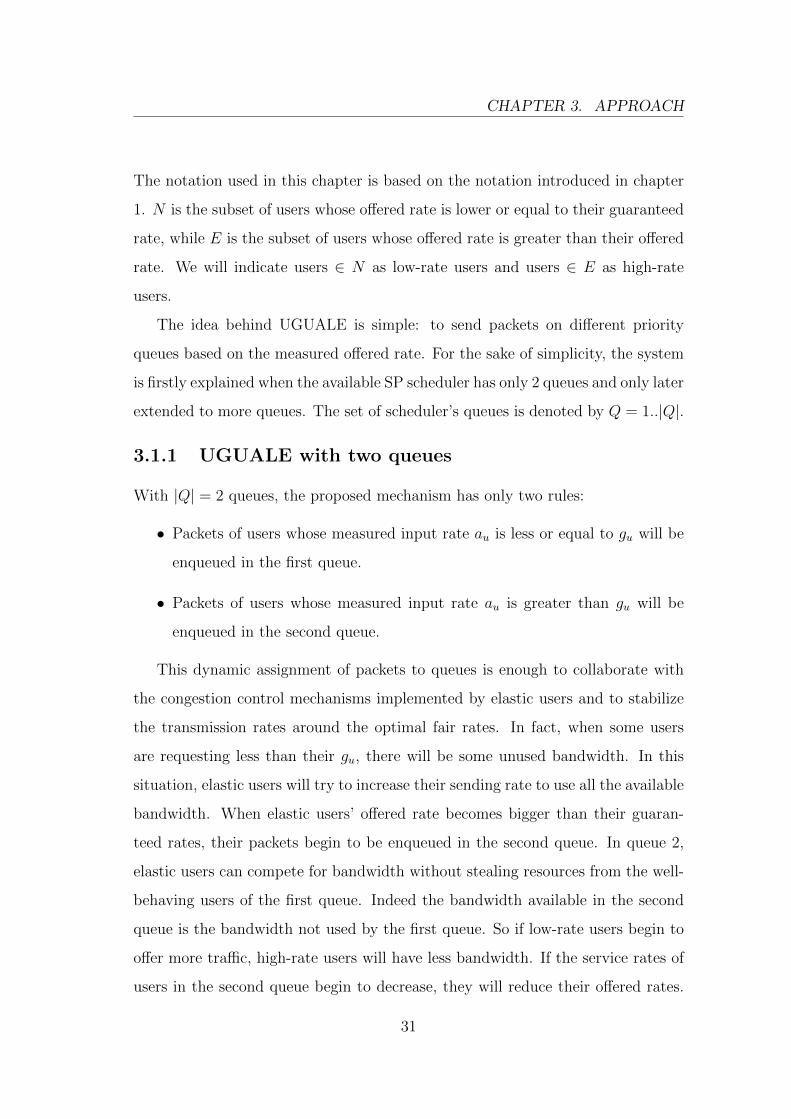
these users will be re-admitted in the first queue. An example of the forwarding
engine with two queues and three users is shown in figure 3.1
a2 ≤ g 2Strict Priority
schedulerLow priority queue
High priority queue
User 1 packet
a3 > g 3
OutputTraffic
a1 > g 1
User 2 packet
User 3 packet
c
Figure 3.1: Example of the UGUALE scheme with |Q| = 2 queues and |U | = 3 users.
With this mechanism, every user will always be able to reach its guaranteed
rate and the throughput of the link is maximized. UGUALE with two queues is
enough to assure guaranteed rates to an arbitrary number of users, but it does not
enforce fairness in the distribution of excess bandwidth. To reach better levels of
fairness and stability, UGUALE can operate with more than two queues.
3.1.2 UGUALE with more queues
As previously mentioned, the UGUALE scheme can be extended to more queues,
so that the more a user increases its rate, the less priority it will get.
For every user u, up to |Q| thresholds can be defined. Thresholds are indicated
by tu,q, where u ∈ U and q ∈ Q. For every user, the first threshold corresponds
to the guaranteed rate and the last threshold corresponds to the link capacity.
The other thresholds are spaced between the first and the last one, as explained
in section 3.3.
The new enqueueing rule is the following: when user u offers a rate au between
thresholds tu,q−1 and tu,q, its packets are enqueued in queue q.
Since there are many thresholds, from now on it is more practical to talk about
bands. Bands are interval of rates between two consecutive thresholds. Band 1
32
CHAPTER 3. APPROACH
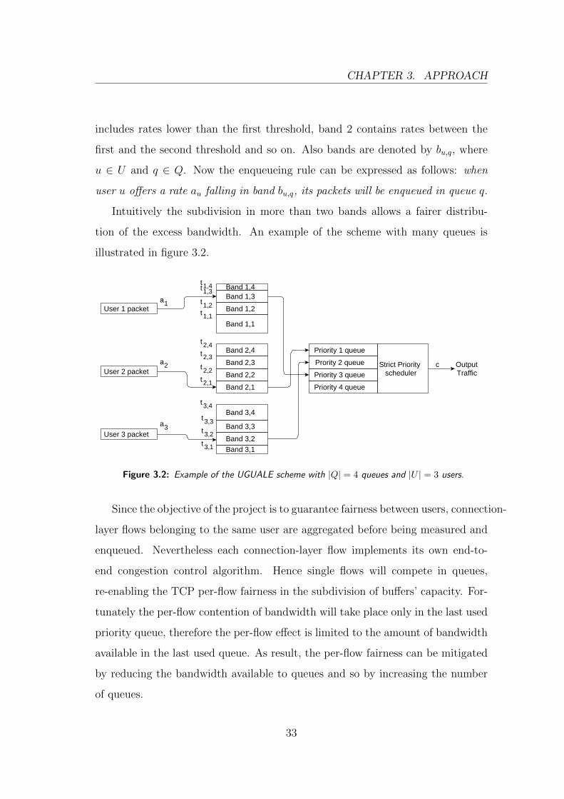
includes rates lower than the first threshold, band 2 contains rates between the
first and the second threshold and so on. Also bands are denoted by bu,q, where
u ∈ U and q ∈ Q. Now the enqueueing rule can be expressed as follows: when
user u offers a rate au falling in band bu,q, its packets will be enqueued in queue q.
Intuitively the subdivision in more than two bands allows a fairer distribu-
tion of the excess bandwidth. An example of the scheme with many queues is
illustrated in figure 3.2.
Band 3,1
Band 2,1
Band 2,2
Band 2,3
Band 2,4
Strict Priorityscheduler
Priority 4 queue
Priority 3 queue
Prority 2 queue
Priority 1 queue
User 1 packet
User 2 packet
User 3 packetBand 3,2
Band 3,3
Band 3,4
Band 1,1
Band 1,2
Band 1,3Band 1,4
OutputTraffic
t1,1
t1,2
t1,3t1,4
t2,1
t2,2
t2,3
t2,4
t3,1
t3,2
t3,3
t3,4
a2
a3
a1
c
Figure 3.2: Example of the UGUALE scheme with |Q| = 4 queues and |U | = 3 users.
Since the objective of the project is to guarantee fairness between users, connection-
layer flows belonging to the same user are aggregated before being measured and
enqueued. Nevertheless each connection-layer flow implements its own end-to-
end congestion control algorithm. Hence single flows will compete in queues,
re-enabling the TCP per-flow fairness in the subdivision of buffers’ capacity. For-
tunately the per-flow contention of bandwidth will take place only in the last used
priority queue, therefore the per-flow effect is limited to the amount of bandwidth
available in the last used queue. As result, the per-flow fairness can be mitigated
by reducing the bandwidth available to queues and so by increasing the number
of queues.
33
CHAPTER 3. APPROACH
3.2 Pipeline
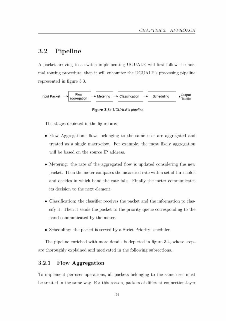
A packet arriving to a switch implementing UGUALE will first follow the nor-
mal routing procedure, then it will encounter the UGUALE’s processing pipeline
represented in figure 3.3.
Input PacketFlow
aggregationMetering Classification Scheduling Output
Traffic
Figure 3.3: UGUALE’s pipeline
The stages depicted in the figure are:
• Flow Aggregation: flows belonging to the same user are aggregated and
treated as a single macro-flow. For example, the most likely aggregation
will be based on the source IP address.
• Metering: the rate of the aggregated flow is updated considering the new
packet. Then the meter compares the measured rate with a set of thresholds
and decides in which band the rate falls. Finally the meter communicates
its decision to the next element.
• Classification: the classifier receives the packet and the information to clas-
sify it. Then it sends the packet to the priority queue corresponding to the
band communicated by the meter.
• Scheduling: the packet is served by a Strict Priority scheduler.
The pipeline enriched with more details is depicted in figure 3.4, whose steps
are thoroughly explained and motivated in the following subsections.
3.2.1 Flow Aggregation
To implement per-user operations, all packets belonging to the same user must
be treated in the same way. For this reason, packets of different connection-layer
34

CHAPTER 3. APPROACH
Input PacketMeasure
Rate
Strict Priority
SchedulerPriority 4 queue
Priority 3 queue
Prority 2 queue
Priority 1 queue
OutputTraffic
Band u,1
Band u,2
Band u,3
Band u,4
tu,1
tu,2
tu,3
tu,4
Meter u
234
1234
1Band Queue
Classification Table
Definitionof user u
Send tometer u
... ...
... ...
Match ActionAggregation table
Flow Aggregation Metering
Classification Scheduling
c
Activated band = 2
Figure 3.4: UGUALE’s detailed pipeline
flows must be aggregated as a single user. Practically, a user must be defined
by a set of rules related to the IP packet header: for instance a user can be
identified by a particular source IP address or by the couple source IP address
and destination TCP port. Therefore the matching fields of the aggregation rules
define users and to each rule corresponds an action to be applied on matching
packets. With UGUALE, the action is sending the packet to a user-dedicated
meter. For example, an aggregation table such as table 3.1 identifies users by the
source IP address and applies a user-specific action.
Match Rule ActionSRC IP = 192.168.1.1 Send to meter 1SRC IP = 192.168.1.2 Send to meter 2
... ...SRC IP = 192.168.1.N Send to meter N
Table 3.1: Example of aggregation table for a system in which users are identified by the sourceIP address. All packets belonging to the same user are sent to a user-dedicated meter.
35

CHAPTER 3. APPROACH
3.2.2 Metering
A meter is a switch element that can take actions based on the measured rate
of packets passing through it. In our scheme, a meter has a set of |Q| bands
defined by |Q| thresholds and each band has an associated action. These actions
are applied when the corresponding bands are activated, i.e. when the measured
rate falls in that band. Since bands are disjoint, a packet can activate only a band.
The meter receives a packet and updates the measured rate. Then the meter
decides to which band the rate belongs to and applies the corresponding action
on the packet: in our case the action is to communicate to the classifier the band
activated by the packet. This communication can be done by associating some
meta-data to the packet.
In our system there is a univocal correspondence between users and meters. In
fact a meter maintains information on the corresponding user, such as the offered
rate, the thresholds and the action. For this reason, UGUALE can manage a
number of users corresponding to the number of meters available in the switch.
3.2.3 Classification
Classification is the act of deciding to which queue a packet should be sent. Gen-
erally, the classification is done based on a packet’s header field, but in our system
it is based on the meta-data written by the meter. So at the end of the pipeline,
the packet will be sent on a certain port of the switch. Every port will have a
multi-queue SP scheduler and a classifier to decide in which queue to send the
packets. The information of the meter band is retrieved by the classifier that fi-
nally puts the packet on a certain queue. To keep the system simple, the classifier
executes a one to one mapping between bands and queues, so that band q will
correspond to queue q.
36

CHAPTER 3. APPROACH
3.2.4 Scheduling
Packets are served by a Strict Priority (SP) scheduler. Since no Active Queue
Management (AQM) is implemented, packets can experience tail drop: a packet
sent to a queue temporarily full will be dropped.
3.3 Thresholds setting
Thresholds must be set in a way that enforces guaranteed rates and fairness. The
rules to distribute bands are elucidated in this section.
3.3.1 First threshold
Since a SP scheduler is used, the only queue that is always able to transmit is
the first one. Moreover, rates lower than the guaranteed ones must always be
assured. To be enqueued in the first queue a user’s rate must remain within its
first threshold, so the first threshold corresponds to the guaranteed rate.
3.3.2 Other thresholds
The other thresholds must be properly set to obtain a fair sharing of the excess
bandwidth. Following the line of thinking of subsection 3.1.2, the dimension of
the bands must be minimized to enhance the control of rates. Since the subset of
bands effectively used in a certain moment is unknown, all bands should be kept
as short as possible. To achieve this principle we chose a uniform distribution: all
thresholds must be equally spaced.
The easiest solution is to assign the first threshold and then to divide the
non-guaranteed bandwidth in |Q| − 1 equal slices, as depicted in figure 3.5. The
non-guaranteed bandwidth of user u is defined as
fu = c− gu ∀u ∈ U
The figure highlights the fact that users will have bands of different width based
37
CHAPTER 3. APPROACH
Band b 1,1
Band b 2,1
Band b 1,3
Band b 1,4
Band b 1,5
Band b 1,6
Band b 1,7
Band b 1,8
Band b 2,2
Band b 2,3
Band b 2,4
Band b 2,5
Band b 2,6
Band b 2,7
Band b 2,8
Band b 1,2
User u=1 User u=2
g1
g2
∆1,q
∆2,q
Figure 3.5: A possible assignment of bands with |Q| = 8 available queues. Bands are obtained bydividing the non-guaranteed bandwidth in |Q| − 1 regular intervals.
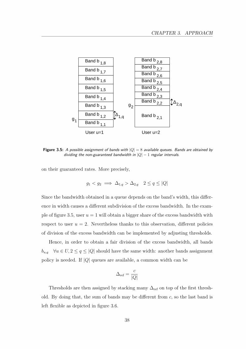
on their guaranteed rates. More precisely,
g1 < g2 =⇒ ∆1,q > ∆2,q 2 ≤ q ≤ |Q|
Since the bandwidth obtained in a queue depends on the band’s width, this differ-
ence in width causes a different subdivision of the excess bandwidth. In the exam-
ple of figure 3.5, user u = 1 will obtain a bigger share of the excess bandwidth with
respect to user u = 2. Nevertheless thanks to this observation, different policies
of division of the excess bandwidth can be implemented by adjusting thresholds.
Hence, in order to obtain a fair division of the excess bandwidth, all bands
bu,q ∀u ∈ U, 2 ≤ q ≤ |Q| should have the same width: another bands assignment
policy is needed. If |Q| queues are available, a common width can be
∆ref =c
|Q|
Thresholds are then assigned by stacking many ∆ref on top of the first thresh-
old. By doing that, the sum of bands may be different from c, so the last band is
left flexible as depicted in figure 3.6.
38

CHAPTER 3. APPROACH
Band 1
Band 2
Band 3
Band 4
Band 5
Band 6
Band 7
Band 8
Band b 1,1
c∆ref =c/|Q|
Band b 1,3
Band b 1,4
Band b 1,5
Band b 1,6
Band b 1,7
Band b 1,8
Referencedistribution
User u=1
g1 Band b 2,1
Band b 2,2
Band b 2,3
Band b 2,4
Band b 2,5
Band b 2,6
Band b 2,7
Band b 2,8
User u=2
g2
Band b 3,2
Band b 3,3
Band b 3,4
Band b 3,5
Band b 3,6
Band b 3,7
User u=3
g3Band b 1,2 Band b 3,1∆ref
Figure 3.6: Assignment of bands with |Q| = 8 available queues. Many ∆ref are stacked on top ofthe guaranteed rate and the last fitting band is adapted to the capacity.
If gu < ∆ref the sum of bands will be smaller than c:
gu < ∆ref =⇒ gu + (|Q| − 1) ·∆ref < c
In this case — user u = 1 in figure 3.6 — it will be necessary to enlarge the last
band. On the contrary, if gu > ∆ref there will be a band that does not fit in the
capacity:
gu > ∆ref =⇒ gu + (|Q| − 1) ·∆ref > c
In this case — users u = 2, 3 in figure 3.6 — the last stacked band will be squeezed
to fit c. If the last fitting band’s index is smaller than |Q|, the following bands
will not be used nor assigned for that user. The index of the last band assigned
to user u is denoted as qu,max ≤ |Q|.
To resume, bands of users are assigned such as
bu,q =
gu q = 1
∆ref 2 ≤ q < qu,max
c−∑
1≤q<qu,maxbu,q q = qu,max
∀u ∈ U
39

CHAPTER 3. APPROACH
3.4 Enhancements
The previously exposed policy to set thresholds assumes only the knowledge of
users’ guaranteed rates. If more information is available, the control on users’
rates can be enhanced using the methods presented in this section.
3.4.1 Ad hoc thresholds
If offered rates are known, the Optimal Fair Rate of users can be calculated as
done in subsection 1.2:
OFRu =
{au ∀u ∈ N
gu + f|E| ∀u ∈ E
where
f = c−∑u∈N
au −∑u∈E
gu
To obtain fairness in this situation it is enough to let the first threshold of user
u correspond to its Optimal Fair Rate OFRu as depicted in figure 3.7.
Band 1
Band 2
c
OFRu
Bands for user u
Figure 3.7: When the OFR of a user is known, a single threshold in the OFR is enough to obtainfairness.
To improve the stability of the system, other bands can be placed around the
OFR threshold, as depicted in figure 3.8. Since bands are placed only in the used
40

CHAPTER 3. APPROACH
c
OFR
(a) (b)
Figure 3.8: When the OFR is known, the assignment of bands (a) can emulate the presence ofmuch more bands (b) because the rates will oscillate only in a small interval.
rates interval, this assignment emulates the presence of much more than |Q| bands
as pointed out in figure 3.8.
Even if this policy might assure the perfect fairness, the system would require
a mechanism that continuously change thresholds based on users’ offered rates:
this proposal seems unpractical and not scalable, so it will be tested only for
theoretical reasons.
3.4.2 Maximum Marking Rate
The UGUALE’s enhancement presented in this subsection assumes the knowledge
of the maximum Optimal Fair Rate. The maximum OFR of the system is:
OFRmax = maxu∈U
OFRu
To obtain its value, offered rates must be known, but the solution proposed does
not require continuous adjustments of thresholds. If the OFRmax is very low
with respect to the link capacity, why bands should be distributed to cover all
41

CHAPTER 3. APPROACH
the link capacity? If the (|Q| − 1)th reference threshold is reduced to a common
value slightly greater than all users’ rates, the ∆ref is reduced, too. That means
enhancing the control on every user’s rate while maintaining the fairness in the
division of the free bandwidth. The new value of the (|Q|−1)th reference threshold
is indicated as the Maximum Marking Rate (MMR) of the system. The MMR
should be large enough to contain the rate of the user having OFRu = OFRmax
and is defined as:
MMR = OFRmax ·|Q| − 1
|Q| − w − 1(3.1)
where w is an integer number representing the number of guard bands. Guard
bands are bands over the OFRmax, without counting the last band. Guard bands
are necessary to contain the oscillations of the highest-rate user and to permit some
flexibility. Without guard bands, if a user reduces its offered rate, the output rates
of other users may grow and users might be regulated by a single large last band.
The optimal number of guard bands will be found experimentally.
From the MMR the new reference width of bands is obtained with the rule
∆ref,MMR =MMR
|Q| − 1=
OFRmax
|Q| − w − 1
as illustrated in figure 3.9
As before, many ∆ref,MMR are stacked on top of the guaranteed rate and the
last used band is adapted to fit the link capacity. Formally,
bu,q =
gu q = 1
∆ref,MMR 2 ≤ q < qu,max
c−∑
1≤q<qu,maxbu,q q = qu,max
∀u ∈ U
3.4.3 Round Trip Time compensation
The UGUALE’s enhancement presented in this subsection assumes the knowledge
of the RTTs of users.
Flows with different RTT competing for the same capacity will obtain different
rates. This aspect should be taken into account because it can notably impact
42

CHAPTER 3. APPROACH
Band 1
Band 2
Band 3
Band 4
Band 5
Band 6
Band 7
Band 8c
Referencedistribution
Band 1
Band 8
c
Referencedistribution
adapted withMMR
Band 2Band 3Band 4Band 5Band 6Band 7 MMR
OFRmax
∆ref ∆ref,MMR
Figure 3.9: Example of bands assignment with the Maximum Marking Rate strategy using w = 4guard bands (in grey).
the fairness of the system. In fact, a difference of RTT is translated in a different
goodput following the relation
goodput1goodputi
≈ RTTi
RTT1
(3.2)
as reported in [16]. With UGUALE it is possible to mitigate this effect by properly
enlarging or shrinking bands by a factor depending from the user’s RTT.
The goodput is defined as the difference between the throughput and the rate
lost for retransmission. For our scope the goodput can be approximated with the
throughput: from now on the goodput will be referred as throughput or rate and
it will be indicated by ru ∀u ∈ U .
Since a user is an arbitrary aggregate of flows, each user’s flow can experience
a different RTT. We define the RTT of a user as the average RTT of its flows.
For each user u ∈ U , we want to find a coefficient mu defined as the factor
that multiplies the estimated rate ru to get the OFRu:
ru ·mu ≡ OFRu ∀u ∈ U
43

CHAPTER 3. APPROACH
We assume that there are N users sharing the same FIFO queue served by a
link of capacity c. We also assume that the users’ RTTs are uniformly distributed
between a minimum and a maximum RTT. Following the relation 3.2 users will
obtain
ru =RTT1
RTTu
· r1 ∀u ∈ U
Fixing r1 = 1, the relation becomes:
ru =RTT1
RTTu
∀u ∈ U
The distribution of rates with r1 = 1,RTT1 = 1 is depicted in figure 3.10.
Assuming that all users deserve the same rate, the optimal fair rate is a con-
50 100 150 200RTT
0.0
0.2
0.4
0.6
0.8
1.0
Rate
Rate dependence from RTT
Theoretical RateOptimal Fair Rate
Figure 3.10: Flows with different RTTs sharing the same FIFO queue obtain different throughputs.There are 200 flows, each one with a different RTT in the range [20,220]
stant:
OFRu =c
N= OFR ∀u ∈ U
The coefficient mu is then
mu =OFR
ru∀u ∈ U
44

CHAPTER 3. APPROACH
By substituting the expressions of the optimal fair rate and of the estimated rate,
we obtain
mu =c · RTTu
N · RTT1 · r1∀u ∈ U
Finally c, N , RTT1 and r1 are constant and can be grouped under a common
factor k, so that the linear dependence of mu from RTTu is highlighted:
mu =c
N · RTT1 · r1· RTTu = k · RTTu ∀u ∈ U
The multiplier is represented in figure 3.11.
50 100 150 200RTT
0.0
0.5
1.0
1.5
2.0
2.5
3.0
Rate
Rate dependence from RTT
Theoretical RateMultiplier
Figure 3.11: The multiplication of the estimated rate by the multiplier produces a straight linecorresponding to the OFR.
The knowledge of users’ RTTs is enough to calculate the coefficient mu of
each user. We suppose that with UGUALE, by multiplying thresholds by these
coefficients, rates of users having different RTTs can be equalized. More precisely,
bands are assigned such that:
bu,q =
gu q = 1
∆ref ·mu 2 ≤ q < qu,max
c−∑
1≤q<qu,maxbu,q q = qu,max
∀u ∈ U
45

CHAPTER 3. APPROACH
Calibration of the multiplier
Multipliers obtained with the method previously proposed may have a too strong
effect when using UGUALE. In fact users are not sharing a simple FIFO queue
and their rates might be already quite similar to their optimal fair rates. For this
reason, the effect of the multiplier can be lightened as depicted in figure 3.12. To
50 100 150 200RTT
0.0
0.5
1.0
1.5
2.0
2.5
3.0
Rate
Rate dependence from RTT
Theoretical RateMultiplier with h=1Multiplier with h=0.2
Figure 3.12: The new multiplier line has a smaller angular coefficient and passes from the pointwhere the old multiplier line is unitary.
reduce the effect of the multiplier, the angular coefficient is multiplied by a factor
0 < h < 1. Moreover, the new multiplier line should pass from the point where
the old multiplier is unitary. If only the angular coefficient k were reduced, all
users will uselessly get a smaller multiplier. If the line were rotated with respect
to another point, all users might get a multiplier greater or bigger than one. The
optimal value of h will be searched experimentally.
46

Chapter 4
Implementation
The approach proposed in the previous chapter was implemented on the real
hardware testbed described in section 4.1. The chosen software switch was picked
following the reasoning presented in section 4.2. The pipeline of UGUALE was
adapted to the testbed and implemented as described in section 4.3. Section 4.4
shows the procedure necessary to obtain a Strict Priority scheduler with Open
vSwitch, while in section 4.5 the implementation of meters is discussed. Section
4.6 shows the softwares used to generate and collect data. Finally, to demon-
strate the effectiveness of UGUALE, an arbitrary number of users with different
characteristics is emulated as described in section 4.7.
4.1 Testbed
UGUALE has been implemented on a physical network in order to have a better
understanding of the available technologies and to discover all the real problems
that can affect computer network communications. This should also demonstrate
the feasibility of our solution.
The testbed was named Redfox and it is composed of five PCs. There are
four Dell Studio XPS 8100, with Intel i7 processor and named Redfox1, Redfox2,
Redfox3 and Redfox4. These PCs are connected through Ethernet CAT6 cables
to a Ciaratech PC, with processor Intel Qual Core 2 running at 3GHz, named
47

CHAPTER 4. IMPLEMENTATION
Redfox0. Redfox0 can act as a software switch thanks to an extra 4-NIC network
interface card, whose ports run at 1Gbps. All PCs run a standard distribution of
the operative system Ubuntu 14.04 LTS. Figure 4.1 shows a picture of the testbed.
Figure 4.1: Photo of the testbed.
The testbed is used with the scheme presented in figure 4.2: Redfox1, Redfox2
and Redfox3 send data to Redfox4. Hence the link (Redfox0, Redfox4) becomes
the bottleneck of the network on which fairness is evaluated. Given this working
scheme, from now on Redfox1, Redfox2 and Redfox3 will be indicated as the client
PCs, Redfox4 as the server and Redfox0 as the switch.
48
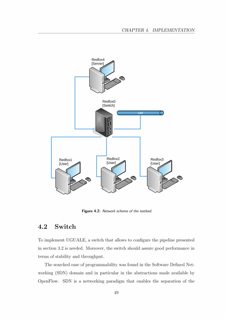
CHAPTER 4. IMPLEMENTATION
LAN
Redfox1[User]
Redfox2[User]
Redfox3[User]
Redfox0[Switch]
Redfox4[Server]
Figure 4.2: Network scheme of the testbed.
4.2 Switch
To implement UGUALE, a switch that allows to configure the pipeline presented
in section 3.2 is needed. Moreover, the switch should assure good performance in
terms of stability and throughput.
The searched ease of programmability was found in the Software Defined Net-
working (SDN) domain and in particular in the abstractions made available by
OpenFlow. SDN is a networking paradigm that enables the separation of the
49

CHAPTER 4. IMPLEMENTATION
control logic from the data plane, while Openflow is the most diffused controller
to data plane interface. OpenFlow compliant switches can be programmed with
a set of instructions that, acting on some abstractions of the physical elements of
the data plane, allow the configuration of the packet pipeline with good flexibility.
Hence, the ideal solution would have been to use a physical OpenFlow compli-
ant switch to have high-performance and compatibility with all the QoS features.
Unfortunately this kind of switches have a prohibitory cost.
We initially thought of implementing the whole testbed in a virtual environ-
ment such as Mininet, but the first simple tests, even with a standard switch
not implementing UGUALE, made clear the instability of the virtual solution in
particular for the evaluation of QoS parameters.
Then we decided to implement the whole system on real machines and to
equip a PC with an extra 4-NICs network card to use it as a software switch.
This solution is notably cheaper than an OpenFlow switch, in fact this kind of
network card costs around 600 CAD. When we got the network card, we replaced
it with the graphic card of a PC and we obtained our switch.
The last step was to find a switching software that could provide all the nec-
essary QoS OpenFlow abstractions and that could guarantee high performance in
terms of total throughput and stability. Although the only OpenFlow abstractions
necessary to implement the proposed scheme are meters and queues, we discovered
that the QoS support in software switches is still limited.
The most popular software switch is Open vSwitch (OVS) [32]. Today it
is widely deployed in data centers because it guarantees high performance and
stability while supporting all QoS features. Unfortunately we discovered that
OVS does not support meters.
Another software switch that we tried is Lagopus [15]. Lagopus implements
OpenFlow 1.3 and is based on the high-performance packet processing library
DPDK (Data Plane Development Kit) [7]. At the time we discovered it, in June
50

CHAPTER 4. IMPLEMENTATION
2015, Lagopus was still at version 0.1.2, supporting meters but not queues.
Another solution that we tried is ofsoftswitch13 [20] that is considered the
reference implementation of OpenFlow: all functionalities are implemented as de-
scribed in the standard. The main drawback is that ofsoftswitch13 is not optimized
for performance, imposing a maximum throughput of only tens on Mbps.
We thought to a workaround: implementing meters directly on client PCs and
using OVS as switching software. In this way we were able to use OVS that was
the only switch guaranteeing high performance and queue programmability.
4.3 Pipeline
The pipeline described in section 3.2 was modified to be executed on our testbed.
In particular the pipeline was adapted to the absence of meters on the switch.
In OpenFlow, a meter is an entity that measures the rate of packets assigned
to it and that applies actions subsequently. Each meter maintains a list of meter
bands, where each band specifies a rate and an action executed only if the packet
is processed with that band. The rate of a band can be specified in Kbit/s or
in packets/s and a meter can also take into account bursts. The action applied
by a band can be drop or remark. The drop action discards the packet while the
remark action marks the DSCP field of the IP packet header. Packets are always
processed by a single band: the meter chooses only the band with the highest
configured rate that is lower than the measured rate. Since the available actions
are only the two just presented, the only way for the meter to communicate to
the classifier which band is activated is to mark the packet.
The pipeline implemented with an OpenFlow compliant switch would look like
the one depicted in figure 4.3.
51

CHAPTER 4. IMPLEMENTATION
Input PacketLookup foroutput portand meter
Meteringand
marking
Lookup foroutputqueue
Scheduling OutputTraffic
Table 1 User's meter Table 2
Figure 4.3: UGUALE’s pipeline with an OpenFlow switch.
The arriving packet is first matched against a table whose fields determine the
output port and define the users. The matching rule appends the chosen output
port to the pipeline of the packet and sends it to the meter dedicated to the
user. The meter chooses a band depending on the measured rate and applies the
correspondent action, that is marking the DSCP field of the packet with a number
corresponding to the band activated. Then the packet is passed to another table
that acts as a classifier for the scheduler: the only matching field is the DSCP
value that corresponds to the queue on which to send the packet. The enqueue
action is appended to the packet’s pipeline that is finally executed.
With the workaround involving meter and marker in the client PC, the pipeline
is quite different and it is represented in figure 4.4.
Input PacketLookup foroutput portand queue
Scheduling OutputTraffic
Table 1
Newpacket
Meteringand
marking
SwitchClient's PC
Figure 4.4: UGUALE’s pipeline when meter and marker are placed in the client PC.
Packets generated by clients are marked just before exiting the network inter-
face. The switch receives the packets and match them against a table whose fields
are the source and destination IP addresses and the DSCP field. The IP address
determines the output port while the DSCP value determines the output queue.
Then the packet’s pipeline is immediately executed.
The meters that we managed to implement on client PCs are not the same
52

CHAPTER 4. IMPLEMENTATION
used in OpenFlow, but the pipeline is still coherent to the proposed approach. In
fact positioning meters at the output interface of client PCs is equivalent to have
them at the input interface of the switch.
4.4 Strict Priority scheduler
OVS supports and implements queues, but the only scheduling policy configurable
with the furnished utility ovs-vsctl is Weighted Round Robin (WRR): we found a
solution also for this problem, as described below.
First of all, using ovs-vsctl, we created a WRR scheduler with |Q| queues
of arbitrary weight. Then, inspecting the kernel configuration with the Traffic
Control (tc) command suite, we noticed that the scheduler was always created
with a fixed reference name ”1:” and its queues were named ”1:1”, ”1:2”, and so
on until ”1:|Q|”. To be precise, scheduler and queues in Linux Kernel are called
respectively Queuing Discipline (qdisc) and classes. The WRR configuration was
useful because it stored references of qdisc and classes in the OVS QoS database.
The next step was to substitute the WRR scheduler with a Strict Priority one.
Indeed thanks to tc commands, we could delete the old htb qdisc whose classes
were automatically destroyed. Then we created a new prio qdisc having the same
reference name ”1:” and |Q| classes. When instantiating a prio qdisc, it is possible
to specify only the number of priority queues |Q| that it should have. These classes
are automatically created with names ranging from ”1:1” to ”1:|Q|”. By default,
the queue with the highest priority is ”1:1” and the lowest one is ”1:|Q|”.
Finally, inspecting the OVS database with the ovs-vsctl utility, we checked
that the references to the qdisc and its classes had not been lost. We executed
some tests specifically designed to verify the correct behavior of the Strict Priority
scheduler and it worked as expected.
53

CHAPTER 4. IMPLEMENTATION
Queue 1
OVS
Queue 2
Queue 3
Queue 4
WeightedRound Robin
Scheduler
1:1
1:2
1:3
1:4
1:
OVS
1:1
1:2
1:3
1:4
1:
Queue 1
OVS
Queue 2
Queue 3
Queue 4
Strict PriorityScheduler
1:1
1:2
1:3
1:4
1:
Linux Kernel
Linux Kernel
Linux Kernel
(a)
(b)
(c)
Figure 4.5: Process to obtain a SP scheduler. A WRR scheduler is created with ovs-vsctl (a). Thenthe scheduler and the queues are deleted with tc commands (b) so that ovs pointersremain valid. Finally the new scheduler and the new queues are created with the samereferences using tc commands (c).
54

CHAPTER 4. IMPLEMENTATION
4.5 Meters
The reference implementation of OpenFlow meters is described in ofsoftswitch13’s
code and it is based on token buckets.
A token bucket is a data structure that enables the comparison of the packet
rate with a given threshold. The bucket collects tokens that arrive with a rate
equivalent to the reference threshold: each token is a grant to transmit a Byte.
When a packet arrives, its size B [Bytes] is compared to the number of tokens T
in the bucket.
• If T − B ≥ 0, B tokens are consumed and the packet rate is considered
below the threshold. The packet is said to be in-profile.
• If T − B < 0, the bucket is voided and the packet rate is considered above
the threshold. The packet is said to be out-of-profile.
A token bucket allows a certain burstiness of the packet rate based on the burst
size parameter. This parameter represents the maximum number of tokens that
the bucket can accumulate.
Packet rate
T-B ≥ 0?
Token rate
B
packetin-profile
T
packetout-profile
Token bucket
Burstsize
yes
no
Figure 4.6: Structure of a token bucket that enables the comparison of the packet rate with athreshold corresponding to the token arrival rate.
In the reference implementation, a meter is implemented like in figure 4.7. For
55

CHAPTER 4. IMPLEMENTATION
Tokenbucketband 4
Tokenbucketband 3
Tokenbucketband 2
Tokenbucketband 1
PacketMaxbandout
Applyaction for
band i
in/out
in/out
in/out
in/out
Band i
Figure 4.7: Scheme of an OpenFlow Meter. The meter has 4 bands.
every band, a token bucket is instantiated. All buckets are periodically refilled at
the same time with a number of tokens based on band rates. In other words, the
token rate corresponds to the band rate. A packet arriving to the meter consumes
tokens from every bucket, then the biggest band with an empty bucket is applied.
While this logic seems easy to implement, we did not find a way to obtain
it in Linux Kernel and with token buckets. Indeed, we proposed two different
implementations of meters: the first uses a cascade of token buckets and the second
uses the rate estimators made available by the Linux Kernel Firewall. The first
solution produces an output marking that is quite different from the OpenFlow
standard while the output of the second solution is more OpenFlow-like, yet not
compliant.
4.5.1 Series of token bucket filters meter
The first solution is illustrated in figure 4.8 and it is totally implemented with
the Linux Kernel suite tc. First of all a DSMARK Queuing Discipline (qdisc) is
instantiated. Even though DSMARK is a qdisc, it does not schedule, reorder or
56
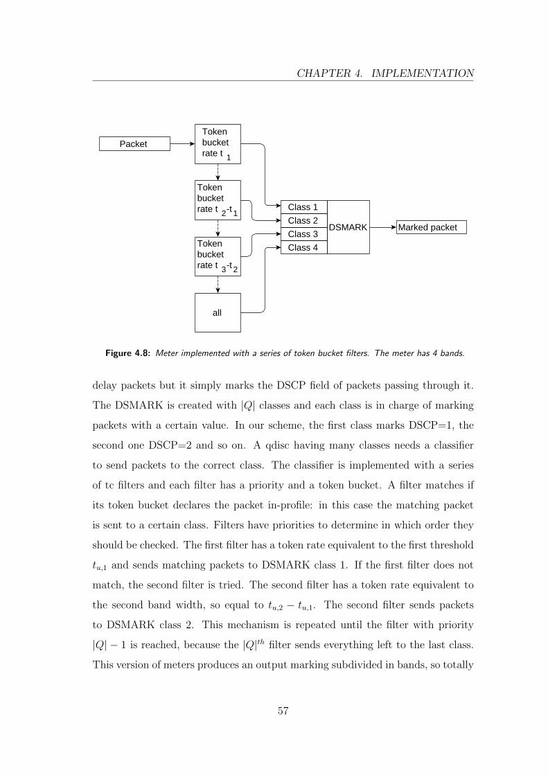
CHAPTER 4. IMPLEMENTATION
DSMARK Marked packet
Class 1
Class 2
Class 3
Class 4
Token bucket rate t 1
Token bucket rate t 2-t 1
Token bucket rate t 3-t 2
all
Packet
Figure 4.8: Meter implemented with a series of token bucket filters. The meter has 4 bands.
delay packets but it simply marks the DSCP field of packets passing through it.
The DSMARK is created with |Q| classes and each class is in charge of marking
packets with a certain value. In our scheme, the first class marks DSCP=1, the
second one DSCP=2 and so on. A qdisc having many classes needs a classifier
to send packets to the correct class. The classifier is implemented with a series
of tc filters and each filter has a priority and a token bucket. A filter matches if
its token bucket declares the packet in-profile: in this case the matching packet
is sent to a certain class. Filters have priorities to determine in which order they
should be checked. The first filter has a token rate equivalent to the first threshold
tu,1 and sends matching packets to DSMARK class 1. If the first filter does not
match, the second filter is tried. The second filter has a token rate equivalent to
the second band width, so equal to tu,2 − tu,1. The second filter sends packets
to DSMARK class 2. This mechanism is repeated until the filter with priority
|Q| − 1 is reached, because the |Q|th filter sends everything left to the last class.
This version of meters produces an output marking subdivided in bands, so totally
57

CHAPTER 4. IMPLEMENTATION
different from the OpenFlow standard.
As an example, a user transmits at a constant bit rate of 400Mbps and has
thresholds at 100Mbps, 200Mbps, 500Mbps and 800Mbps. With this kind of
meters the 25% of packets are marked as 1, another 25% are marked as 2 and
the remaining 50% are marked as 3. According to the OpenFlow standard these
packets should be all marked as 3. The example is depicted in figure 4.9.
t1=100Mbps
t2=200Mbps
t3=500Mbps
t4=800Mbps
Input trafficCBR 400Mbps
3 3 3 3
OpenFlow meter
t1=100Mbps
t2=200Mbps
t3=500Mbps
t4=800Mbps
3 3 2 1
Token b. meter
3 3 2 1
3 3 3 3
Input trafficCBR 400Mbps
(a)
(b)
Output packets DSCP
Output packets DSCP
Figure 4.9: Example showing the output of different meter implementations.
4.5.2 Iptables estimator meter
To obtain an OpenFlow-like behavior, we tried the implementation of meters
illustrated in figure 4.10. This version uses the Linux Kernel Firewall suite iptables
and the tc suite. First of all, a DSMARK qdisc and its classes are configured as
58

CHAPTER 4. IMPLEMENTATION
DSMARKrate> t 1all
Class 4
Class 3
Class 2
Class 1
Estimator
Marked packet
Packet
rate> t 2
rate> t 3
Figure 4.10: Meter implemented with an iptables estimator. The meter has 4 bands.
before. Then a firewall table is populated with an estimator and two rules for
each class.
Every table of iptables is composed of rules, and every rule has a matching
criterion and an action called target. The target is applied only if the packet
matches the rule. A packet is compared with all rules from the top to the bottom
until it encounters the target ACCEPT. This target lets the packet pass to an
eventual next table or to the Linux Kernel.
The first rule matches every packet and sends them to an estimator. Then,
for each class two rules are written:
1. The first rule compares the rate of the estimator with a threshold. If the
estimated rate is greater than the threshold, the packet matches and the
CLASSIFY target is applied. This action classifies the packet: it decides on
which DSMARK class the packet should be sent.
2. The second rule has the same matching criterion of the previous one, but it
applies the ACCEPT target.
Since we check if a rate is greater than a threshold, the first couple of rules has
thresholds corresponding to the (|Q| − 1)th band and sends packets to the |Q|th
class. All rules until the second band are specified in the same way. Also in this
case, the last rule is different because it will match everything left. The estimator
has a minimum measurement interval of 250ms with a Logarithmic Estimated
Weighted Moving Average (ewma-log) of 500ms. For this reason this meter does
not produce an output completely equivalent to the reference implementation.
59
CHAPTER 4. IMPLEMENTATION
4.6 Collecting data
To generate data and collect statistics we used two softwares: iPerf and Band-
width Monitor Next Generation (bwm-ng).
IPerf allows to establish TCP and UDP connections between two sockets and to
send data for the desired amount of time. The process receiving data is indicated
as the iPerf server, while the sender is called client. A client can open an arbitrary
number of parallel connections to the server. If TCP connections are used, the
transmitting rate is the maximum permitted by the network: for this reason iPerf
is commonly used to test links capacity. When using UDP connections, a sending
rate must be specified. This rate, if supported by the network, is maintained for
all the time specified. Both the server and the client processes produce reports
about the actual goodput of flows. These reports are produced with an arbitrary
time period. If a client opens parallel connections to a server, iPerf produces
client-aggregated reports.
Bwm-ng is a tool that reliably monitors the current bandwidth of network
interfaces in a specified direction. Bwm-ng produces reports with an arbitrary
time period and was used to check the total rate received by the server.
To have an immediate idea about the rates obtained by users, we needed a
tool to gather and visualize in real-time the reports generated by the mentioned
softwares. For this reason we wrote a Python script named plotServer that in-
stantiates many iPerf server processes and a bwm-ng process and then starts to
plot the reports received. A screenshot of plotServer is presented in figure 4.11.
The figure is composed of two subplots:
• The first one shows raw samples produced by iPerf aggregated by source
IP address and protocol. Connections from the same IP address of differ-
ent protocols are plotted with the same color but with different line styles.
In particular, continuous lines are used for TCP connections, while UDP
connections are represented by dashed lines. This plot shows also the raw
60

CHAPTER 4. IMPLEMENTATION
10 20 30 40 50 600.0
20.0M
40.0M
60.0M
80.0M
100.0M
bit/s
Per-user TCP/UDP raw rate2 users
SUM192.168.200.1192.168.200.2
10 20 30 40 50 600.0
20.0M
40.0M
60.0M
80.0M
100.0M
bit/s
Per-user smoothed rate (8s window)
Figure 4.11: Screenshot of plotServer with two users having both TCP and UDP connections.Users are defined only by the source IP address. In the first subplot, continuous linesrepresents TCP flows while dashed lines UDP flows. In the time interval [8sec,15sec],the difference between the goodput obtained by a TCP flow and the interface rate isobservable.
bwm-ng reports labeled as ”SUM”.
• The second subplot shows the total rate obtained by users, where a user is
only defined by the source IP address. Lines are smoothed by a weighted
moving average algorithm.
To execute many test cases with different users’ configurations, we wrote an-
other Python script called test that:
1. Configures the UGUALE’s pipeline on the switch.
2. Configures client PCs, e.g. by instantiating meters and markers.
3. Starts the plotServer script.
61
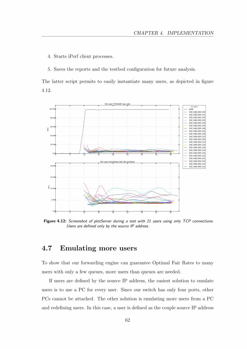
CHAPTER 4. IMPLEMENTATION
4. Starts iPerf client processes.
5. Saves the reports and the testbed configuration for future analysis.
The latter script permits to easily instantiate many users, as depicted in figure
4.12.
0 5 10 15 20 25 30 35 400.0
20.0M
40.0M
60.0M
80.0M
100.0M
bit/s
Per-user TCP/UDP raw rate21 users
SUM192.168.200.130192.168.200.131192.168.200.133192.168.200.132192.168.200.134192.168.200.135192.168.200.136192.168.200.124192.168.200.126192.168.200.123192.168.200.120192.168.200.113192.168.200.110192.168.200.116192.168.200.114192.168.200.115192.168.200.122192.168.200.121192.168.200.125192.168.200.112192.168.200.111
0 5 10 15 20 25 30 35 400.0
5.0M
10.0M
15.0M
20.0M
bit/s
Per-user smoothed rate (8s window)
Figure 4.12: Screenshot of plotServer during a test with 21 users using only TCP connections.Users are defined only by the source IP address.
4.7 Emulating more users
To show that our forwarding engine can guarantee Optimal Fair Rates to many
users with only a few queues, more users than queues are needed.
If users are defined by the source IP address, the easiest solution to emulate
users is to use a PC for every user. Since our switch has only four ports, other
PCs cannot be attached. The other solution is emulating more users from a PC
and redefining users. In this case, a user is defined as the couple source IP address
62
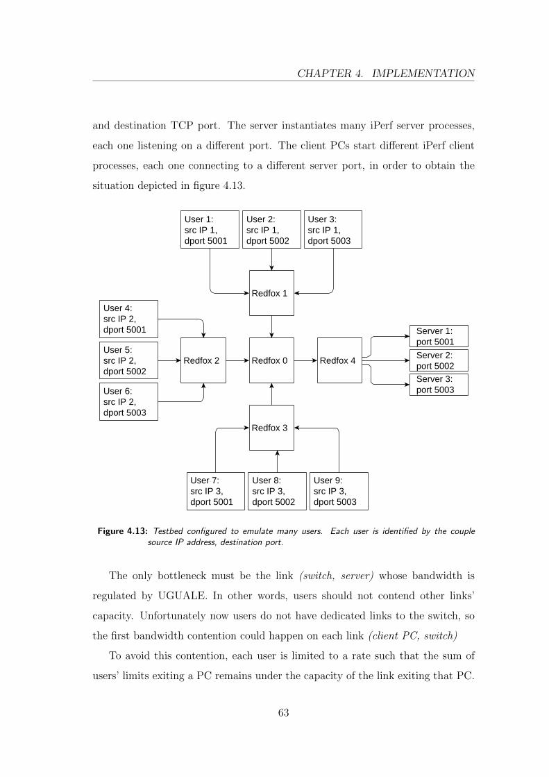
CHAPTER 4. IMPLEMENTATION
and destination TCP port. The server instantiates many iPerf server processes,
each one listening on a different port. The client PCs start different iPerf client
processes, each one connecting to a different server port, in order to obtain the
situation depicted in figure 4.13.
User 7: src IP 3, dport 5001
User 8: src IP 3, dport 5002
User 9: src IP 3, dport 5003
Redfox 0 Redfox 4
User 1: src IP 1, dport 5001
User 2: src IP 1, dport 5002
User 3: src IP 1, dport 5003
User 4: src IP 2, dport 5001
User 5: src IP 2, dport 5002
User 6: src IP 2, dport 5003
Server 1: port 5001
Server 2: port 5002
Server 3: port 5003
Redfox 1
Redfox 2
Redfox 3
Figure 4.13: Testbed configured to emulate many users. Each user is identified by the couplesource IP address, destination port.
The only bottleneck must be the link (switch, server) whose bandwidth is
regulated by UGUALE. In other words, users should not contend other links’
capacity. Unfortunately now users do not have dedicated links to the switch, so
the first bandwidth contention could happen on each link (client PC, switch)
To avoid this contention, each user is limited to a rate such that the sum of
users’ limits exiting a PC remains under the capacity of the link exiting that PC.
63
CHAPTER 4. IMPLEMENTATION
Then also the link (switch, server) should be limited to the same value, otherwise
it would not be the bottleneck: each user would obtain a rate corresponding to its
first limit. Formally, the emulated users and the bottleneck must be limited link
such that ∑u∈Ui
cu ≤ li ∀i ∈ I
cu = c ∀u ∈ U
where
• I is the set of PCs
• Ui is the set of users emulated on PC i ∈ I
• cu is the link bottleneck capacity for the emulated user u.
• li is the capacity of the link (i,switch)
• c is the bottleneck link capacity
The first constraint says that the total capacity available for users of the same
PC cannot be greater than the capacity of the link exiting the PC itself. The
second constraint puts the obtained capacity to a common value corresponding to
the bottleneck link capacity. To avoid perturbations, the bottleneck negotiates a
capacity of c=100Mbps. Since li = 1Gbps ∀i ∈ I, the maximum number of users
per PC is li/c = 10 ∀i ∈ I.
If all users would start to transmit at the same time, the capacity of the
bottleneck link would be the first to be contended, so it would not be strictly
necessary to limit users’ processes.
4.7.1 Emulating users with different Round Trip Times
To reproduce the situation of users with different Round Trip Times (RTTs)
described in subsection 3.4.3, a tool to delay processes is needed.
64

CHAPTER 4. IMPLEMENTATION
It possible to delay processes with softwares but the output is not realistic at
all. E.g. using Trickle, processes simply get throttled for regular time intervals,
modifying completely the TCP behavior.
A better solution is to use NetEm, that is able to delay and rate limit packets.
As reported in [10], the TCP sequence and windows obtained using NetEm are
very similar to the ones obtained with real links. NetEm is a Queueing Discipline
(qdisc) available in the tc suite, so it must be attached to an egress interface or
to another qdisc. The latter option is easy but unsuitable for our tests: the only
types of qdisc allowing to attach more than one qdisc are classful qdiscs. Classful
qdiscs are schedulers with more than one queue. In this case, each NetEm can
be attached to a different queue. This solution modifies the fairness between
emulated users because packets get scheduled for transmission on the real link
(client PC, switch) with an order different from FIFO. In other words, a classful
qdisc would begin to schedule its queues and all the emulated users would get
perfectly the same rate.
A solution that does not alter the bandwidth sharing between users is to attach
a NetEm to virtual interfaces (veth). Virtual interfaces must be linked to the real
Ethernet interface using an internal bridge. The internal bridge can be the default
Linux bridge or an instance of Open vSwitch (OVS). We chose OVS because it
seems more stable and because it does not apply any implicit fairness mechanism
between its ports. In this way, users are served as if they were flowing into a single
FIFO queue.
Another problem was to make packets generated by different processes pass
through different veths based on the definition of user. This problem was solved
using iptables, ip rules and routing tables together, as depicted in figure 4.14 and
described below:
1. The packet is generated in the main user space, with a certain destination
TCP port.
65

CHAPTER 4. IMPLEMENTATION
2. The packet is managed by the firewall (iptables), where it receives a firewall
mark based on the destination port.
3. Thanks to ip rule the packet is sent to a certain routing table based on the
carried firewall mark.
4. Each routing table contains a single entry that directs all packets to a certain
veth, to which a NetEm is attached.
Passing through a NetEm, the packet is delayed. If the PC is implementing also
meters and markers, the packet is marked when passing through the DSMARK
qdisc attached to the physical interface eth0.
66

CHAPTER 4. IMPLEMENTATION
eth0
veth1 veth2 veth3
InternalOVS
NetEmdelay1
DSMARK
dport fw mark
5001 1
5002 2
5003 3
iptables
fw mark
ip rule
routing table
1 1
2 2
3 3
routing table 1
default: veth1
routing table 2
default: veth2
routing table 3
default: veth3
NetEmdelay2
NetEmdelay3
output traffic
Generated packet
Figure 4.14: PC configuration to emulate many users with different delays.
67
Chapter 5
Experimental results
Section 5.1 describes how tests were executed and how data was validated, ana-
lyzed and presented. In section 5.2 the results obtained are showed and commented
to clarify the functioning of UGUALE.
5.1 Test
A test is defined by the configuration of the testbed and by the data collected
by the server using that configuration. The data consists in a set of rate samples
for every user. Each sample is identified by the time stamp (ts) in which the
sample was produced and by the value of the user’s rate (val) in that instant. The
structure of a test file is depicted in figure 5.1
The testbed is configured as shown in figure 4.13: Redfox0 is the switch,
Redfox4 executes several iPerf server processes and the other PCs act as iPerf
clients. Since the client PCs send data to the server, the link (Redfox0, Redfox4)
becomes the bottleneck on which fairness is evaluated. UGUALE will be used
only on the switch port of the bottleneck link toward the server. In the opposite
direction (from the server to the client PCs) there will be only flows of TCP ACKs
that for certain do not consume enough bandwidth to saturate the links’ capacity.
68

CHAPTER 5. EXPERIMENTAL RESULTS
Figure 5.1: Structure of a test file
5.1.1 Test validation
The data collected during the tests must be validated before proceeding with the
analysis. To evaluate fairness, all rate samples must belong to the same time
interval in which all users are in a steady state. In each test, the server processes
start at time t0 while the client processes start after a fixed time interval necessary
to transmit and apply the particular test configuration to the client PCs. All the
timestamps of a test are relative to its t0.
To declare a test valid:
• The number of recorded users must be equal to the number of instantiated
users.
• All users must begin to transmit within an instant indicated by tstart.
• All users must be still active at the end of the test, when the server processes
are stopped. This instant is indicated by tend.
• All users must produce approximately the same number of rate samples in
the interval [tstart, tend].
69

CHAPTER 5. EXPERIMENTAL RESULTS
• Every user can have just a few low rate samples, i.e. periods in which
transmission was interrupted.
The first instant tstart was set to 35 seconds. This interval is quite large since rates
become stable within a couple of seconds, but it is ensures that all connections
started and reached a stable rate. The final instant tend was set to 3 seconds
before the end of the test, so that all samples are taken strictly before the end of
transmissions. If the test is valid, data can be recorded and analyzed.
5.1.2 Data analysis
First of all, data is trimmed in order to consider only the rate samples falling in
the time interval [tstart, tend]. Then many statistics are calculated.
Jain’s Fairness Index To evaluate the fairness between users, the Jain’s Fair-
ness Index (JFI) can be used [23]. The Jain’s Fairness Index is defined as:
f(r1, r2, ...r|U |) =(∑
u∈U xu)2
|U | ·∑
u∈U x2u
where xu is the normalized throughput of a user u. The normalized throughput is
defined as the ratio between the measured throughput ru and the fair throughput
OFRu of a user u:
xu =ru
OFRu
This index is bounded between 0 and 1, where 1 is a fair distribution and 0 is
a discriminating one. The Jain’s Fairness Index can be calculated with the rate
allocation vector taken in different instants or with average rates. The first option
allows to evaluate also the variance of the JFI, but since iPerf does not produce
synchronized samples, the allocation vectors can be obtained only by interpolating
and re-sampling data at fixed time instants.
Throughput and goodput Another aspect to evaluate is the total link utiliza-
tion. For each instant of the previous re-sampling, the goodput is obtained as the
70

CHAPTER 5. EXPERIMENTAL RESULTS
sum of the allocation vector elements while the throughput samples are obtained
from the bwm-ng reports. Both the goodput and the throughput samples are nor-
malized with respect to the bottleneck link capacity c. Finally, to calculate the
ratio goodput/throughput in various time instants, also the throughput samples
should be interpolated and re-sampled. For all of the presented link utilization
indexes, the mean and the variance are calculated.
Data transformation To further analyze data, each raw sample ru,t of user u
at time t is transformed with the function
g(ru,t,OFRu, c) =ru,t −OFRu
c
The sample is related to the OFR, enabling the comparison between users with
different guaranteed rates and thus different OFRs. The normalization with re-
spect to the bottleneck capacity allows to express rates in the bounded interval
[−1,+1]. For instance, a transformed rate equal to 0 means that the raw rate is
equal to the OFR, while a transformed rate equal to −0.1 means that the raw
rate is the 10% lower than the OFR with respect to the bottleneck capacity.
To be precise, the assignment of guaranteed rates and the estimation of the
OFRs consider the maximum goodput achievable on the link instead of the nom-
inal link capacity. If it were not so, when all users offer their guaranteed rates no
one will be able to reach it. The practical link capacity is the maximum rate that
iPerf reports when only an elastic user is transmitting on the link. For instance
on 100 Mbps links the practical capacity was c = 94.1 Mbps.
5.1.3 Data presentation
Each test is presented in a figure composed of four subplots and a text box, e.g.
figure 5.2. The statistics exhibited in the subplots are calculated on transformed
rates. The figure is organized as follows:
71
CHAPTER 5. EXPERIMENTAL RESULTS
• Subplot (a) shows the discrete distribution of samples. The transformed
samples of all users are joined in a single list on which histograms and other
statistics are computed. Histograms count the occurrences of values grouped
by intervals called bins. In our case, the space of rates [−1,+1] was divided
in 500 symmetric bins.
• Subplot (b) shows the average and the standard deviation of users’ rates. In
this graph, users are ordered by ID (e.g. the IP address) in order to show
details about single users.
• Subplot (c) shows average and standard deviation of transformed rates for
users aggregated by the number of TCP connections. This subplot allows
to evaluate the dependence of rates from the number of TCP connections.
• Subplot (d) shows average and standard deviation of transformed rates for
users aggregated by RTT. This subplot allows to evaluate the dependence
of rates from the RTT.
• The text-box is divided in three sections. The first section lists the ID, the
number of TCP connections and the RTT of each user. The second and
third sections report respectively the configuration and other statistics of
the test.
To resume, the presented statistics are:
• The mean and the variance of the Jain’s Fairness Index.
• The mean and the variance of the throughput.
• The mean and the variance of the goodput.
• The mean and the variance of the ratio between the goodput and the
throughput.
72
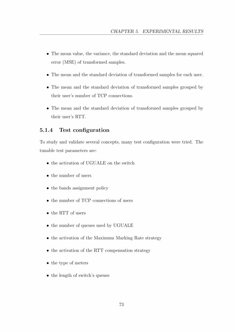
CHAPTER 5. EXPERIMENTAL RESULTS
• The mean value, the variance, the standard deviation and the mean squared
error (MSE) of transformed samples.
• The mean and the standard deviation of transformed samples for each user.
• The mean and the standard deviation of transformed samples grouped by
their user’s number of TCP connections.
• The mean and the standard deviation of transformed samples grouped by
their user’s RTT.
5.1.4 Test configuration
To study and validate several concepts, many test configuration were tried. The
tunable test parameters are:
• the activation of UGUALE on the switch
• the number of users
• the bands assignment policy
• the number of TCP connections of users
• the RTT of users
• the number of queues used by UGUALE
• the activation of the Maximum Marking Rate strategy
• the activation of the RTT compensation strategy
• the type of meters
• the length of switch’s queues
73

CHAPTER 5. EXPERIMENTAL RESULTS
5.1.5 Outline of tests
The first step is to run tests without UGUALE to evaluate the basic behavior of
the testbed. For this purpose OVS in standalone fail-mode is used: the switch
executes the standard MAC learning and does not enforce QoS policies. In this
configuration, when all users are in the same conditions (that is when all users
have the same number of TCP connections and the same RTT) they should obtain
the same rate. This case can be considered as a baseline, in other words as the
target fairness that the testbed can achieve. By contrast, executing tests with
users in different conditions is useful to show the TCP per-flow fairness and the
impairments caused by different RTTs.
The second step is to run tests with UGUALE to prove that the conditions
presented in section 1.2 are enforced. To verify that the guaranteed rates are
assured,∑
u gu should be set equal to c (free bandwidth equal to zero) and users
should be set in different conditions. Then, by increasing the free bandwidth, the
fairness in the allocation of the excess capacity can be evaluated. Finally other
tests can be executed to verify the effectiveness of the enhancements proposed in
section 3.4 and to calibrate their parameters.
74

CHAPTER 5. EXPERIMENTAL RESULTS
5.2 Results
This section presents the obtained results and observations about the texts exe-
cuted.
5.2.1 Switch in standalone fail-mode
When the switch is in standalone fail-mode, QoS is not enforced and fairness
depends on users’ conditions. In particular, three different situations can occur:
• If all users have the same number of TCP connections and the same RTT,
every user obtains the same throughput and the JFI is very high. This
situation, represented in figure 5.2, constitutes a baseline and demonstrates
the stability of the testbed.
• If users have a different number of TCP connections, the TCP per-flow
fairness shows up and the per-user fairness is impaired. The relation be-
tween the number of TCP connections and the rate obtained is linear, as
highlighted in figure 5.3(c).
• If users have different Round Trip Times, the fairness is impaired as dis-
cussed in subsection 3.4.3: rates are inversely proportional to the RTT, as
shown in figure 5.4(d).
The latter two situations, in which the JFI drops to approximately 0.8, explain
why a QoS enforcing mechanism like UGUALE is necessary.
75

CHAPTER 5. EXPERIMENTAL RESULTS
3N. of TCP connections
0.10
0.05
0.00
0.05
0.10
Dist
ance
from
OFR
nor
mal
ized
w.r.
t. bo
ttlen
eck
capa
city
(c)
Mean/std
40.0RTT [ms]
0.10
0.05
0.00
0.05
0.10 (d)
Mean/std
1 11 21User ID
0.10
0.05
0.00
0.05
0.10
Dist
ance
from
OFR
nor
mal
ized
w.r.
t. bo
ttlen
eck
capa
city
(b)
Mean/std
-0.15 0 0.15Distance from OFR normalized
w.r.t. bottleneck capacity
0
10
20
30
40
50
Disc
rete
dis
trib
utio
n
Mean: 0.0000291Var: 0.0000665Std: 0.0081561MSE: 0.0000665
(a)
Mean USERSUser 1: 3c, 40msUser 2: 3c, 40msUser 3: 3c, 40msUser 4: 3c, 40msUser 5: 3c, 40msUser 6: 3c, 40msUser 7: 3c, 40msUser 8: 3c, 40msUser 9: 3c, 40msUser 10: 3c, 40msUser 11: 3c, 40msUser 12: 3c, 40msUser 13: 3c, 40msUser 14: 3c, 40msUser 15: 3c, 40msUser 16: 3c, 40msUser 17: 3c, 40msUser 18: 3c, 40msUser 19: 3c, 40msUser 20: 3c, 40msUser 21: 3c, 40ms
CONFIGURATIONSwitch type: standaloneSwitch queue lenght: 126 pkt
STATISTICSJain's Index mean: 0.9720768Jain's Index var: 0.0000746Throughput mean: 0.9870592Throughput var: 0.0000003Goodput mean: 0.9414216Goodput var: 0.0000227Ratio G/T mean: 0.9537642Ratio G/T var: 0.0000232
Figure 5.2: When all users have the same number of TCP connections and the same RTT, QoSenforcing is not necessary to obtain fairness.
76
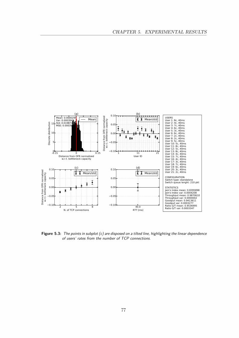
CHAPTER 5. EXPERIMENTAL RESULTS
2 5 8N. of TCP connections
0.10
0.05
0.00
0.05
0.10
Dist
ance
from
OFR
nor
mal
ized
w.r.
t. bo
ttlen
eck
capa
city
(c)
Mean/std
40.0RTT [ms]
0.10
0.05
0.00
0.05
0.10 (d)
Mean/std
1 11 21User ID
0.10
0.05
0.00
0.05
0.10
Dist
ance
from
OFR
nor
mal
ized
w.r.
t. bo
ttlen
eck
capa
city
(b)
Mean/std
-0.15 0 0.15Distance from OFR normalized
w.r.t. bottleneck capacity
0
5
10
15
Disc
rete
dis
trib
utio
n
Mean: 0.0000299Var: 0.0003949Std: 0.0198714MSE: 0.0003949
(a)
Mean USERSUser 1: 8c, 40msUser 2: 4c, 40msUser 3: 7c, 40msUser 4: 6c, 40msUser 5: 3c, 40msUser 6: 6c, 40msUser 7: 2c, 40msUser 8: 2c, 40msUser 9: 5c, 40msUser 10: 5c, 40msUser 11: 8c, 40msUser 12: 5c, 40msUser 13: 8c, 40msUser 14: 4c, 40msUser 15: 7c, 40msUser 16: 4c, 40msUser 17: 3c, 40msUser 18: 7c, 40msUser 19: 6c, 40msUser 20: 3c, 40msUser 21: 2c, 40ms
CONFIGURATIONSwitch type: standaloneSwitch queue lenght: 210 pkt
STATISTICSJain's Index mean: 0.8395898Jain's Index var: 0.0004208Throughput mean: 0.9870610Throughput var: 0.0000002Goodput mean: 0.9413611Goodput var: 0.0003277Ratio G/T mean: 0.9536995Ratio G/T var: 0.0003347
Figure 5.3: The points in subplot (c) are disposed on a tilted line, highlighting the linear dependenceof users’ rates from the number of TCP connections.
77
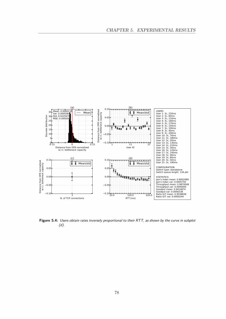
CHAPTER 5. EXPERIMENTAL RESULTS
3N. of TCP connections
0.10
0.05
0.00
0.05
0.10
Dist
ance
from
OFR
nor
mal
ized
w.r.
t. bo
ttlen
eck
capa
city
(c)
Mean/std
20.0 120.0 220.0RTT [ms]
0.10
0.05
0.00
0.05
0.10 (d)
Mean/std
1 11 21User ID
0.10
0.05
0.00
0.05
0.10
Dist
ance
from
OFR
nor
mal
ized
w.r.
t. bo
ttlen
eck
capa
city
(b)
Mean/std
-0.15 0 0.15Distance from OFR normalized
w.r.t. bottleneck capacity
0
5
10
15
20
25
30
35
Disc
rete
dis
trib
utio
n
Mean: 0.0000139Var: 0.0005084Std: 0.0225478MSE: 0.0005084
(a)
Mean USERSUser 1: 3c, 220msUser 2: 3c, 60msUser 3: 3c, 110msUser 4: 3c, 160msUser 5: 3c, 170msUser 6: 3c, 150msUser 7: 3c, 100msUser 8: 3c, 40msUser 9: 3c, 200msUser 10: 3c, 70msUser 11: 3c, 180msUser 12: 3c, 20msUser 13: 3c, 130msUser 14: 3c, 210msUser 15: 3c, 30msUser 16: 3c, 120msUser 17: 3c, 140msUser 18: 3c, 90msUser 19: 3c, 80msUser 20: 3c, 50msUser 21: 3c, 190ms
CONFIGURATIONSwitch type: standaloneSwitch queue lenght: 126 pkt
STATISTICSJain's Index mean: 0.8002089Jain's Index var: 0.0005750Throughput mean: 0.9870048Throughput var: 0.0000000Goodput mean: 0.9414874Goodput var: 0.0000238Ratio G/T mean: 0.9538836Ratio G/T var: 0.0000244
Figure 5.4: Users obtain rates inversely proportional to their RTT, as shown by the curve in subplot(d).
78
CHAPTER 5. EXPERIMENTAL RESULTS
5.2.2 UGUALE
The results presented in figures 5.5 and 5.6 show that the proposed allocation
engine is able to assure guaranteed rates to a big number of users in different
conditions.
2 5 8N. of TCP connections
0.10
0.05
0.00
0.05
0.10
Dist
ance
from
OFR
nor
mal
ized
w.r.
t. bo
ttlen
eck
capa
city
(c)
Mean/std
40.0RTT [ms]
0.10
0.05
0.00
0.05
0.10 (d)
Mean/std
1 11 21User ID
0.10
0.05
0.00
0.05
0.10
Dist
ance
from
OFR
nor
mal
ized
w.r.
t. bo
ttlen
eck
capa
city
(b)
Mean/std
-0.15 0 0.15Distance from OFR normalized
w.r.t. bottleneck capacity
010203040506070
Disc
rete
dis
trib
utio
n
Mean: -0.0000775Var: 0.0000311Std: 0.0055744MSE: 0.0000311
(a)
Mean USERSUser 1: 7c, 40msUser 2: 4c, 40msUser 3: 2c, 40msUser 4: 2c, 40msUser 5: 5c, 40msUser 6: 5c, 40msUser 7: 6c, 40msUser 8: 6c, 40msUser 9: 8c, 40msUser 10: 7c, 40msUser 11: 3c, 40msUser 12: 7c, 40msUser 13: 4c, 40msUser 14: 4c, 40msUser 15: 6c, 40msUser 16: 3c, 40msUser 17: 2c, 40msUser 18: 8c, 40msUser 19: 3c, 40msUser 20: 8c, 40msUser 21: 5c, 40ms
CONFIGURATIONSwitch type: ugualeMarking type: iptablesSwitch queue lenght: 210 pktUnused capacity: 0.0N. of bands: 8N. of guard bands: -1RTT compensation: False
STATISTICSJain's Index mean: 0.9902083Jain's Index var: 0.0000112Throughput mean: 0.9870587Throughput var: 0.0000002Goodput mean: 0.9393858Goodput var: 0.0001669Ratio G/T mean: 0.9517010Ratio G/T var: 0.0001707
Figure 5.5: UGUALE is able to assure guaranteed rates to users having a different number of TCPconnections: the points in subplot (c) remain on the horizontal axis.
79

CHAPTER 5. EXPERIMENTAL RESULTS
3N. of TCP connections
0.10
0.05
0.00
0.05
0.10
Dist
ance
from
OFR
nor
mal
ized
w.r.
t. bo
ttlen
eck
capa
city
(c)
Mean/std
20.0 120.0 220.0RTT [ms]
0.10
0.05
0.00
0.05
0.10 (d)
Mean/std
1 11 21User ID
0.10
0.05
0.00
0.05
0.10
Dist
ance
from
OFR
nor
mal
ized
w.r.
t. bo
ttlen
eck
capa
city
(b)
Mean/std
-0.15 0 0.15Distance from OFR normalized
w.r.t. bottleneck capacity
0
20
40
60
80
100
Disc
rete
dis
trib
utio
n
Mean: 0.0000074Var: 0.0000324Std: 0.0056928MSE: 0.0000324
(a)
Mean USERSUser 1: 3c, 180msUser 2: 3c, 60msUser 3: 3c, 170msUser 4: 3c, 40msUser 5: 3c, 200msUser 6: 3c, 160msUser 7: 3c, 220msUser 8: 3c, 30msUser 9: 3c, 50msUser 10: 3c, 150msUser 11: 3c, 140msUser 12: 3c, 70msUser 13: 3c, 190msUser 14: 3c, 100msUser 15: 3c, 90msUser 16: 3c, 120msUser 17: 3c, 20msUser 18: 3c, 110msUser 19: 3c, 80msUser 20: 3c, 210msUser 21: 3c, 130ms
CONFIGURATIONSwitch type: ugualeMarking type: iptablesSwitch queue lenght: 126 pktUnused capacity: 0.0N. of bands: 2N. of guard bands: -1RTT compensation: False
STATISTICSJain's Index mean: 0.9868650Jain's Index var: 0.0000236Throughput mean: 0.9870126Throughput var: 0.0000000Goodput mean: 0.9411788Goodput var: 0.0001692Ratio G/T mean: 0.9535632Ratio G/T var: 0.0001732
Figure 5.6: UGUALE is able to assure guaranteed rates to users having different RTTs: the pointsin subplot (d) remain on the horizontal axis.
When there is no free bandwidth, users oscillate around their first threshold
and rates are almost perfectly controlled. To test how the free bandwidth is shared,
the OFRs of users should be bigger than their guaranteed rates. To emulate this
situation, the sum of guaranteed rates of active users must be lower than c. Since
thresholds are assigned using the rules presented in section 3.3, bands are c/|Q|
wide and rate oscillations can be that big. In the unlucky case where the OFR
is far from thresholds, all packets are regulated by the same band and they end
up in the same queue, so fairness cannot improve significantly with respect to the
standalone case.
To confirm this idea and to clarify how the width of bands influences the
amplitude of rate oscillations, the bands assignment illustrated in figure 5.7 was
tried with several central band’s widths. Since the OFR should fall exactly in the
80
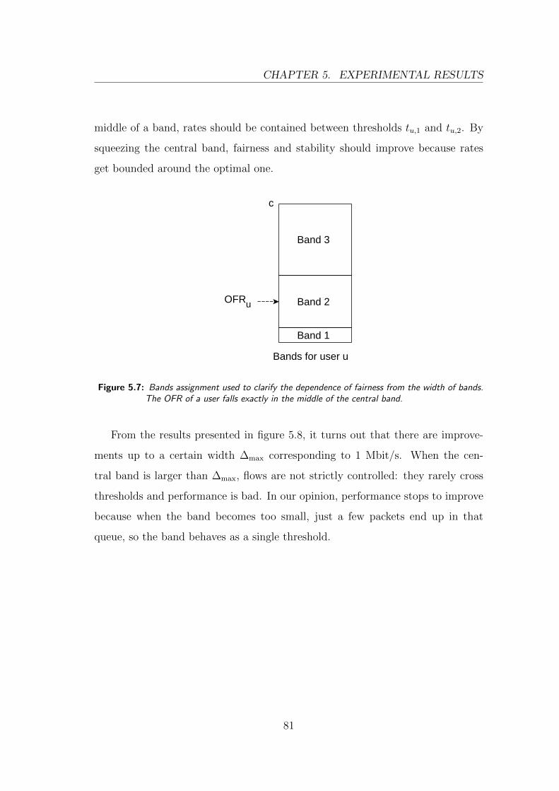
CHAPTER 5. EXPERIMENTAL RESULTS
middle of a band, rates should be contained between thresholds tu,1 and tu,2. By
squeezing the central band, fairness and stability should improve because rates
get bounded around the optimal one.
Band 1
Band 3
c
OFRu
Bands for user u
Band 2
Figure 5.7: Bands assignment used to clarify the dependence of fairness from the width of bands.The OFR of a user falls exactly in the middle of the central band.
From the results presented in figure 5.8, it turns out that there are improve-
ments up to a certain width ∆max corresponding to 1 Mbit/s. When the cen-
tral band is larger than ∆max, flows are not strictly controlled: they rarely cross
thresholds and performance is bad. In our opinion, performance stops to improve
because when the band becomes too small, just a few packets end up in that
queue, so the band behaves as a single threshold.
81

CHAPTER 5. EXPERIMENTAL RESULTS
1.00E+001.00E+011.00E+021.00E+031.00E+041.00E+051.00E+061.00E+071.00E+080.88
0.90
0.92
0.94
0.96
0.98
1.00
Central band width [bit/s]
Jain
's F
airn
ess
Inde
x m
ean
1.00E+001.00E+011.00E+021.00E+031.00E+041.00E+051.00E+061.00E+071.00E+080.00E+00
1.00E-04
2.00E-04
3.00E-04
4.00E-04
5.00E-04
6.00E-04
7.00E-04
Central band width [bit/s]
Jain
's F
airn
ess
Inde
x va
rianc
e
Figure 5.8: The graphs shows the mean and the variance of the Jain’s Fairness Index dependingon the width of the central band. Statistics were obtained using the band assignmentdepicted in figure 5.7 and 9 users having a different number of TCP connections. Atest was executed for each central width. The unitary width corresponds to a singlethreshold in the OFR.
82

CHAPTER 5. EXPERIMENTAL RESULTS
5.2.3 UGUALE with ad hoc thresholds
To exploit the band assignment proposed in subsection 3.4.1, the offered rates of
users must be known. Hence, this scheme were tried to test:
• if a single threshold in the OFR is enough to assure fairness
• if other bands can be concentrated around the OFR threshold to increase
fairness and stability
The results, presented in figure 5.9, show that generally performance does not
improve significantly by adding bands around the OFR threshold. When the
packets of a user are spread on too many queues, performance drops, e.g. when
small bands (125 Kbit/s, 250Kbit/s and 500Kbit/s) are used. On the contrary,
adding bands that will not be used is useless, as in the case of large bands (2
Mbit/s and 4 Mbit/s): at a certain point, performance remains stationary. In
conclusion, each flow should be regulated by not more than 4 bands at a time,
since this is the point that obtains the best fairness and stability. This rule of
thumb determines the optimal band’s width ∆opt, that in our case is still equal to
1 Mbit/s.
83

CHAPTER 5. EXPERIMENTAL RESULTS
2 4 6 8 10 120.98
0.982
0.984
0.986
0.988
0.99
0.992
0.994
0.996
0.998
1
125 Kbit/s250 Kbit/s500 Kbit/s1 Mbit/s2 Mbit/s4 Mbit/s
Jain
's F
airn
ess
Inde
x m
ean
Central bands'width
(a)
2 4 6 8 10 120
0.000005
0.00001
0.000015
0.00002
0.000025
0.00003
Number of bands
Jain
's F
airn
ess
Inde
x va
rianc
e
(b)
Band 1
Band 2
OFRBand 2Band 3 Band 4
Band 5
Band 2Band 3 Band 4
Band 5
Band 2Band 3
Band 6Band 7
Band 4Band 5
Band 2Band 3
Band 6Band 7Band 8Band 9
Band 4Band 5
Band 2Band 3
Band 6Band 7Band 8Band 9
Band 10Band 11
Band 1
Band 4
Band 1
Band 6
Band 1
Band 8
Band 1
Band 10
Band 1
Band 12
OFR
(c)
Figure 5.9: The graphs shows the mean and the variance of the Jain’s Fairness Index dependingon the width of the central bands. Statistics were obtained using the band assignmentdepicted in sub-figure (c) and 9 users having a different number of TCP connections.
84

CHAPTER 5. EXPERIMENTAL RESULTS
5.2.4 UGUALE with MMR
When the maximum Optimal Fair Rate is known, the Maximum Marking Rate
strategy presented in subsection 3.4.2 can be applied. Since bands in the used
range are small with respect to the basic case, UGUALE assures an excellent per-
user fairness even in the free bandwidth case. As shown in figures 5.10 and 5.11,
fairness is guaranteed to users having a different number of TCP connections or
a different RTT.
2 5 8N. of TCP connections
0.10
0.05
0.00
0.05
0.10
Dist
ance
from
OFR
nor
mal
ized
w.r.
t. bo
ttlen
eck
capa
city
(c)
Mean/std
40.0RTT [ms]
0.10
0.05
0.00
0.05
0.10 (d)
Mean/std
1 11 21User ID
0.10
0.05
0.00
0.05
0.10
Dist
ance
from
OFR
nor
mal
ized
w.r.
t. bo
ttlen
eck
capa
city
(b)
Mean/std
-0.15 0 0.15Distance from OFR normalized
w.r.t. bottleneck capacity
0
10
20
30
40
50
60
70
Disc
rete
dis
trib
utio
n
Mean: -0.0000517Var: 0.0000341Std: 0.0058431MSE: 0.0000341
(a)
Mean USERSUser 1: 4c, 40msUser 2: 7c, 40msUser 3: 5c, 40msUser 4: 3c, 40msUser 5: 5c, 40msUser 6: 8c, 40msUser 7: 2c, 40msUser 8: 3c, 40msUser 9: 6c, 40msUser 10: 7c, 40msUser 11: 8c, 40msUser 12: 3c, 40msUser 13: 7c, 40msUser 14: 4c, 40msUser 15: 4c, 40msUser 16: 6c, 40msUser 17: 2c, 40msUser 18: 6c, 40msUser 19: 5c, 40msUser 20: 8c, 40msUser 21: 2c, 40ms
CONFIGURATIONSwitch type: ugualeMarking type: iptablesSwitch queue lenght: 210 pktUnused capacity: 0.5N. of bands: 8N. of guard bands: 5RTT compensation: False
STATISTICSJain's Index mean: 0.9903255Jain's Index var: 0.0000110Throughput mean: 0.9870071Throughput var: 0.0000000Goodput mean: 0.9401060Goodput var: 0.0001846Ratio G/T mean: 0.9524812Ratio G/T var: 0.0001896
Figure 5.10: UGUALE with the MMR strategy improves the fairness of users having a differentnumber of TCP connections even in presence of free bandwidth: the points in subplot(c) remain on the horizontal axis.
The only parameter to optimize was the number of guard bands. In all the test
configurations tried, the best results were obtained using w = 4 or w = 5 guard
bands out of |Q| = 8 total bands: these values make one of the first thresholds fall
closer to the OFR. If less guard bands are used, the bands’ width results to small
and the rates above the OFR will not be regulated. If more guard bands are used,
85

CHAPTER 5. EXPERIMENTAL RESULTS
3N. of TCP connections
0.10
0.05
0.00
0.05
0.10
Dist
ance
from
OFR
nor
mal
ized
w.r.
t. bo
ttlen
eck
capa
city
(c)
Mean/std
20.0 120.0 220.0RTT [ms]
0.10
0.05
0.00
0.05
0.10 (d)
Mean/std
1 11 21User ID
0.10
0.05
0.00
0.05
0.10
Dist
ance
from
OFR
nor
mal
ized
w.r.
t. bo
ttlen
eck
capa
city
(b)
Mean/std
-0.15 0 0.15Distance from OFR normalized
w.r.t. bottleneck capacity
0
20
40
60
80
Disc
rete
dis
trib
utio
n
Mean: -0.0002898Var: 0.0000434Std: 0.0065846MSE: 0.0000434
(a)
Mean USERSUser 1: 3c, 200msUser 2: 3c, 60msUser 3: 3c, 190msUser 4: 3c, 210msUser 5: 3c, 110msUser 6: 3c, 160msUser 7: 3c, 150msUser 8: 3c, 180msUser 9: 3c, 40msUser 10: 3c, 50msUser 11: 3c, 70msUser 12: 3c, 220msUser 13: 3c, 130msUser 14: 3c, 100msUser 15: 3c, 120msUser 16: 3c, 170msUser 17: 3c, 90msUser 18: 3c, 30msUser 19: 3c, 20msUser 20: 3c, 140msUser 21: 3c, 80ms
CONFIGURATIONSwitch type: ugualeMarking type: iptablesSwitch queue lenght: 126 pktUnused capacity: 0.5N. of bands: 8N. of guard bands: 5RTT compensation: False
STATISTICSJain's Index mean: 0.9853120Jain's Index var: 0.0001721Throughput mean: 0.9870789Throughput var: 0.0000002Goodput mean: 0.9350705Goodput var: 0.0002698Ratio G/T mean: 0.9473338Ratio G/T var: 0.0002769
Figure 5.11: UGUALE with the MMR strategy improves the fairness of users having different RTTseven in presence of free bandwidth: the points in subplot (d) remain on the horizontalaxis.
bands remain large and performance does not improve significantly (with respect
to the no-MMR case) because wide oscillations are still permitted.
86
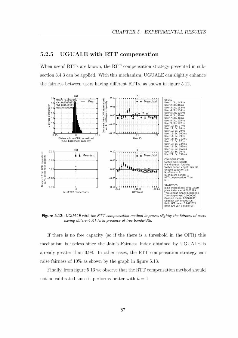
CHAPTER 5. EXPERIMENTAL RESULTS
5.2.5 UGUALE with RTT compensation
When users’ RTTs are known, the RTT compensation strategy presented in sub-
section 3.4.3 can be applied. With this mechanism, UGUALE can slightly enhance
the fairness between users having different RTTs, as shown in figure 5.12,
3N. of TCP connections
0.10
0.05
0.00
0.05
0.10
Dist
ance
from
OFR
nor
mal
ized
w.r.
t. bo
ttlen
eck
capa
city
(c)
Mean/std
20.0 115.0 210.0RTT [ms]
0.10
0.05
0.00
0.05
0.10 (d)
Mean/std
1 11 21User ID
0.10
0.05
0.00
0.05
0.10
Dist
ance
from
OFR
nor
mal
ized
w.r.
t. bo
ttlen
eck
capa
city
(b)
Mean/std
-0.15 0 0.15Distance from OFR normalized
w.r.t. bottleneck capacity
0
5
10
15
20
25
30
35
Disc
rete
dis
trib
utio
n
Mean: -0.0001955Var: 0.0002083Std: 0.0144343MSE: 0.0002084
(a)
Mean USERSUser 1: 3c, 143msUser 2: 3c, 86msUser 3: 3c, 153msUser 4: 3c, 134msUser 5: 3c, 115msUser 6: 3c, 58msUser 7: 3c, 48msUser 8: 3c, 105msUser 9: 3c, 172msUser 10: 3c, 77msUser 11: 3c, 96msUser 12: 3c, 29msUser 13: 3c, 200msUser 14: 3c, 39msUser 15: 3c, 210msUser 16: 3c, 67msUser 17: 3c, 124msUser 18: 3c, 181msUser 19: 3c, 162msUser 20: 3c, 20msUser 21: 3c, 191ms
CONFIGURATIONSwitch type: ugualeMarking type: iptablesSwitch queue lenght: 126 pktUnused capacity: 0.5N. of bands: 8N. of guard bands: -1RTT compensation: Trueh: 1
STATISTICSJain's Index mean: 0.9119550Jain's Index var: 0.0002299Throughput mean: 0.9870069Throughput var: 0.0000000Goodput mean: 0.9369281Goodput var: 0.0002406Ratio G/T mean: 0.9492624Ratio G/T var: 0.0002469
Figure 5.12: UGUALE with the RTT compensation method improves slightly the fairness of usershaving different RTTs in presence of free bandwidth.
If there is no free capacity (so if the there is a threshold in the OFR) this
mechanism is useless since the Jain’s Fairness Index obtained by UGUALE is
already greater than 0.98. In other cases, the RTT compensation strategy can
raise fairness of 10% as shown by the graph in figure 5.13.
Finally, from figure 5.13 we observe that the RTT compensation method should
not be calibrated since it performs better with h = 1.
87

CHAPTER 5. EXPERIMENTAL RESULTS
0.0 0.2 0.4 0.6 0.8 1.0 1.20.76
0.78
0.80
0.82
0.84
0.86
0.88
0.90
0.92
0.94
0.96
0.98
1.00
0
0.2
0.4
0.6
h
Jain
's F
airn
ess
Ind
ex M
ean
Unusedcapacity
Figure 5.13: Variation of the Jain’s Fairness Index based on the multiplier h applied to the RTTcompensation strategy. There are 21 users, each one with 3 TCP connections, withRTT uniformly distributed between 20ms and 220ms. Note that with h = 0, the RTTcompensation strategy is not applied.
5.2.6 Type of meter
In section 4.5 two different implementations of meters were discussed. UGUALE
enforces fairness with both implementations, but statistics are different.
The first meter type, implemented with a series of token bucket filters, produces
an output subdivided in bands even for constant rate flows: consecutive packets
can be marked differently and thus end up in different queues. This might cause
packet reordering and so many packet retransmissions.
The second type of meter, implemented with a rate estimator, ensures that
as long as the rate remains constant, packets are marked in the same way. This
meter might cause less packet reordering, but when the offered rate oscillates
around a threshold, consecutive bursts of packets receive different priorities and
the reactiveness of the control might decrease.
These considerations are confirmed by test results: the token bucket implemen-
tation causes a small degradation of the goodput with respect to the estimator
case. The goodput reduction affects all users in the same way, so the fairness
remains high but the mean rates are lower than expected. Nevertheless, the to-
88
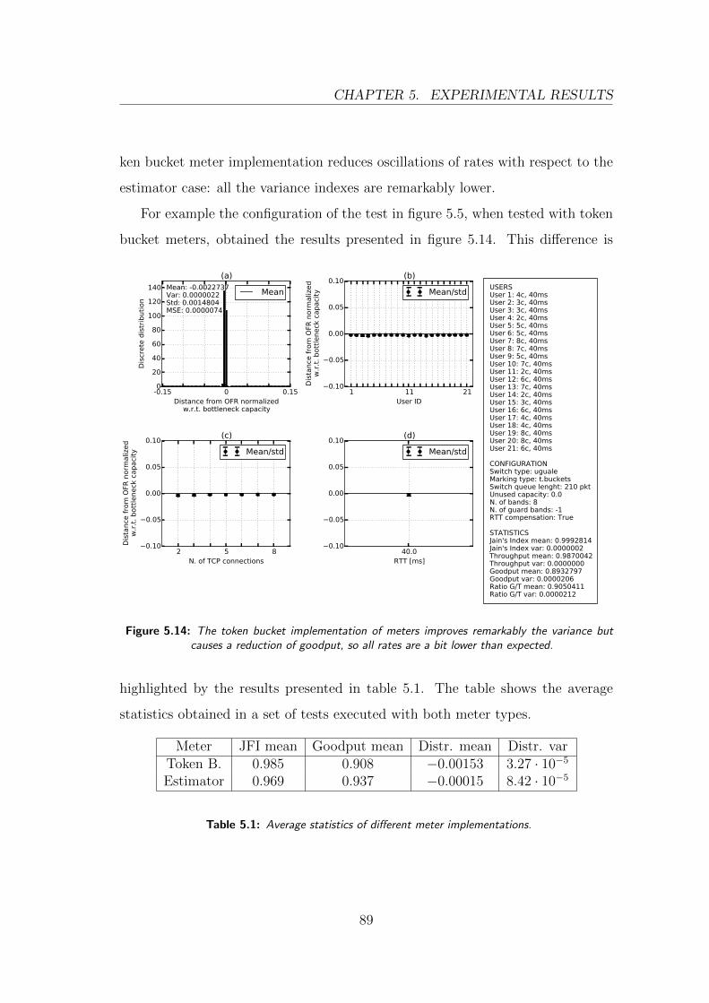
CHAPTER 5. EXPERIMENTAL RESULTS
ken bucket meter implementation reduces oscillations of rates with respect to the
estimator case: all the variance indexes are remarkably lower.
For example the configuration of the test in figure 5.5, when tested with token
bucket meters, obtained the results presented in figure 5.14. This difference is
2 5 8N. of TCP connections
0.10
0.05
0.00
0.05
0.10
Dist
ance
from
OFR
nor
mal
ized
w.r.
t. bo
ttlen
eck
capa
city
(c)
Mean/std
40.0RTT [ms]
0.10
0.05
0.00
0.05
0.10 (d)
Mean/std
1 11 21User ID
0.10
0.05
0.00
0.05
0.10
Dist
ance
from
OFR
nor
mal
ized
w.r.
t. bo
ttlen
eck
capa
city
(b)
Mean/std
-0.15 0 0.15Distance from OFR normalized
w.r.t. bottleneck capacity
0
20
40
60
80
100
120
140
Disc
rete
dis
trib
utio
n
Mean: -0.0022737Var: 0.0000022Std: 0.0014804MSE: 0.0000074
(a)
Mean USERSUser 1: 4c, 40msUser 2: 3c, 40msUser 3: 3c, 40msUser 4: 2c, 40msUser 5: 5c, 40msUser 6: 5c, 40msUser 7: 8c, 40msUser 8: 7c, 40msUser 9: 5c, 40msUser 10: 7c, 40msUser 11: 2c, 40msUser 12: 6c, 40msUser 13: 7c, 40msUser 14: 2c, 40msUser 15: 3c, 40msUser 16: 6c, 40msUser 17: 4c, 40msUser 18: 4c, 40msUser 19: 8c, 40msUser 20: 8c, 40msUser 21: 6c, 40ms
CONFIGURATIONSwitch type: ugualeMarking type: t.bucketsSwitch queue lenght: 210 pktUnused capacity: 0.0N. of bands: 8N. of guard bands: -1RTT compensation: True
STATISTICSJain's Index mean: 0.9992814Jain's Index var: 0.0000002Throughput mean: 0.9870042Throughput var: 0.0000000Goodput mean: 0.8932797Goodput var: 0.0000206Ratio G/T mean: 0.9050411Ratio G/T var: 0.0000212
Figure 5.14: The token bucket implementation of meters improves remarkably the variance butcauses a reduction of goodput, so all rates are a bit lower than expected.
highlighted by the results presented in table 5.1. The table shows the average
statistics obtained in a set of tests executed with both meter types.
Meter JFI mean Goodput mean Distr. mean Distr. varToken B. 0.985 0.908 −0.00153 3.27 · 10−5
Estimator 0.969 0.937 −0.00015 8.42 · 10−5
Table 5.1: Average statistics of different meter implementations.
89
CHAPTER 5. EXPERIMENTAL RESULTS
5.3 Length of switch queues
A parameter that impact fairness and stability is the length of switch queues. If
queues are long, packets have a big latency and the end-to-end congestion control
mechanisms cannot react in short times. Generally, this causes unfairness and
wide rate oscillations. By contrast, short queues keep the variance and the latency
low. The default Linux queue length (1000 packets for each NIC) is too big for
our testbed configuration. In fact, the best results were obtained when the queue
lengths were set with the rule presented in [8]:
L =RTT · c√
n[bit]
where:
• RTT is the average RTT of users
• c is the link capacity
• n is the number of TCP flows on the link
Since even UGUALE improved using this rule, it was used in all tests presented.
Only when users have different RTTs, long queues enhance the fairness. In
fact, the different reactiveness of users’ end-to-end congestion control is smoothed
and so the JFI is higher with respect to the equivalent case having short queues.
An example is presented in figure 5.15: the test in figure 5.4 was repeated with
long queues and fairness improved significantly.
90

CHAPTER 5. EXPERIMENTAL RESULTS
3N. of TCP connections
0.10
0.05
0.00
0.05
0.10
Dist
ance
from
OFR
nor
mal
ized
w.r.
t. bo
ttlen
eck
capa
city
(c)
Mean/std
20.0 120.0 220.0RTT [ms]
0.10
0.05
0.00
0.05
0.10 (d)
Mean/std
1 11 21User ID
0.10
0.05
0.00
0.05
0.10
Dist
ance
from
OFR
nor
mal
ized
w.r.
t. bo
ttlen
eck
capa
city
(b)
Mean/std
-0.15 0 0.15Distance from OFR normalized
w.r.t. bottleneck capacity
0
10
20
30
40
Disc
rete
dis
trib
utio
n
Mean: 0.0000191Var: 0.0001155Std: 0.0107450MSE: 0.0001155
(a)
Mean USERSUser 1: 3c, 150msUser 2: 3c, 210msUser 3: 3c, 20msUser 4: 3c, 200msUser 5: 3c, 120msUser 6: 3c, 220msUser 7: 3c, 110msUser 8: 3c, 70msUser 9: 3c, 90msUser 10: 3c, 50msUser 11: 3c, 30msUser 12: 3c, 60msUser 13: 3c, 100msUser 14: 3c, 130msUser 15: 3c, 180msUser 16: 3c, 190msUser 17: 3c, 40msUser 18: 3c, 80msUser 19: 3c, 170msUser 20: 3c, 140msUser 21: 3c, 160ms
CONFIGURATIONSwitch type: standaloneSwitch queue lenght: 1000 pkt
STATISTICSJain's Index mean: 0.9487407Jain's Index var: 0.0003195Throughput mean: 0.9870039Throughput var: 0.0000000Goodput mean: 0.9411627Goodput var: 0.0001463Ratio G/T mean: 0.9535551Ratio G/T var: 0.0001502
Figure 5.15: Test without QoS enforcing, where users have different RTTs and the switch has longqueues.
91
Chapter 6
Conclusion
Bandwidth sharing is still an issue in todays networks, since it is difficult to
provide fairness to a large number of users while fully exploiting the links’ capacity.
As discussed in the document, there are several solutions but they are either
complicate to set up or not scalable, so practically the problem remains unsolved
and Internet is still Best Effort oriented.
The bandwidth sharing problem was formally defined and the current ap-
proaches were analyzed in order to propose an original solution. The new band-
width allocation scheme (UGUALE) works by dynamically assigning users to the
queues of a Strict Priority scheduler, based on the measured input rate. In par-
ticular, the more traffic is offered, the less priority is obtained. This assignment
interacts with the end-to-end congestion control mechanisms implemented by users
and stabilizes the output rates around the desired ones. Since there are no the-
oretical models involving dynamic queue assignment, we decided to first assess
the approach using experiments. To do so, a real testbed composed of five PCs
was set up and one of those PCs was adapted to operate as the switch hosting
UGUALE. The bandwidth sharing scheme was implemented using the abstrac-
tions made available by the OpenFlow switch model and APIs. Finally, in order
to perform tests and collect data, several automation and monitoring scripts were
written.
The results show that when bandwidth sharing is not enforced by the net-
92

CHAPTER 6. CONCLUSION
work, users obtain a rate proportional to their number of TCP connections and
inversely proportional to their RTT. By contrast, with UGUALE, users obtain
their guaranteed rates, no matter the number of TCP connections instantiated
or the RTT of their flows. We noticed that the fairness in the assignment of the
spare capacity depends on the number and width of used bands. Hence, with a
simple enhancement that concentrate thresholds close to the used rate interval,
even the free bandwidth is optimally redistributed to elastic users. Moreover we
observed that the goodput and the stability of rates are influenced by the type of
meters and that performance depends on the length of switch queues.
In summary, the proposed allocation engine proved to be very effective in
guaranteeing minimum rates and in the fair repartition of the excess bandwidth
among users. In fact, UGUALE allows an easy assignment of bandwidth shares
to users and the maximum link utilization using only the instruments already
available in modern switches. In conclusion, the promising results obtained by
UGUALE makes us believe that such an approach is worth of further analysis.
6.1 Future works
The proposed forwarding engine performs well in tested situations, but further
cases and aspects need to be evaluated.
In static cases, users do not change their behavior during the test and the
system is evaluated in a steady state. Until now, only a set of static cases have
been examined but many others are necessary:
• A scalability test to discover the maximum number of users supported. The
number of users should be increased until the performance drops signifi-
cantly.
• Tests where users have different types of congestion control mechanisms
(including inelastic users).
93

CHAPTER 6. CONCLUSION
• Tests that clarify the effect of meters’ parameters on performance. In par-
ticular, the update frequency of the estimator (for iptables meters) and the
burst size (for token bucket meters) should be investigated.
• Tests using a real OpenFlow switch to verify the behavior of UGUALE with
OpenFlow meters.
Moreover, other QoS parameters can be evaluated, such as delay and jitter. Then
the dynamic performance of UGUALE should be studied by executing:
• Tests where the number of active users varies in time to evaluate the conver-
gence time of rates to the OFR. Users should implement different congestion
control mechanisms.
• Tests with realistic TCP traffic, i.e. composed of a combination of ele-
phant and mice flows. Elephant flows emulate bulk transfers, as the long-
lived connections already tested wit iPerf. By contrast, mice flows emulate
HTTP traffic that is usually composed of many short bursts. Mice flows are
very short-lived and end up transmissions before reaching their Slow Start
Threshold (SSTHRESH). For this reason, other parameter such as the Flow
Completion Time (FCT) can be considered.
Leaving the single node problem, the utilization of UGUALE in a network must
be considered. More precisely, the network architecture to embrace it should be
defined.
The first architectural option is to run UGUALE on every network node, so
that fairness is guaranteed on each link. This solution might present some scal-
ability and management issues, since all routers should know users’ guaranteed
rates and meter all packets.
Another option is to run UGUALE only on edge routers thus leaving a stateless
version in core routers. Core routers should send packets on different queues based
on the band previously chosen by edge routers. The band should be communicated
94

CHAPTER 6. CONCLUSION
to the core routers by writing some data in the packet header, e.g. by marking
the DSCP field. Nevertheless, to obtain fairness all packets sharing a link should
be marked consistently. This solution seems more practical since it resembles the
well-known DiffServ architecture.
In both the sketched architectures, a centralized control of the network is
necessary to set thresholds in a coherent way. This control can be enforced using
the standard network engineering protocols or more simply in the SDN domain.
Moreover, if a reactive control mechanism were available, thresholds could be
periodically tuned based on the network traffic so to enhance the performance of
the system.
95


Bibliography
[1] K. Ramakrishnan A. Manin. Gateway congestion control survey. IETF RFC
(Informational) 1254, aug 1991.
[2] S. Floyd A. Medina, M. Allman. Measuring the evolution of transport pro-
tocols in the internet. ACM SIGCOMM Computer Communication Review
35, no.2, apr 2005.
[3] Scott Shenker Alan Demers, Srinivasan Keshavt. Analysis and simulation of
a fair queueing algorithm. aug 1989.
[4] Grenville Armitage. Quality of service in ip networks. New Riders Publishing,
nov 2001.
[5] Bob Briscoe. Flow rate fairness: Dismantling a religion. apr 2007.
[6] Robert Morris Dong Lin. Dynamics of random early detection. acm, 1997.
[7] DPDK. Data plane development kit: what it is. http://dpdk.org.
[8] N. McKeown G. Appenzeller, I. Keslassy. Sizing router buffers. SIG-
COMM’04, 2004.
[9] Sujata Banerjee Gwyn Chatranon, Miguel A. Labrador. Black: Detection
and preferential dropping of high bandwidth unresponsive flows. 2003.
[10] Stephen Hemminger. Network emulation with netem. apr 2005.
97
BIBLIOGRAPHY
[11] Hui Zhang Ion Stoica, Scott Shenker. Core-stateless fair queueing: A scal-
able architecture to approximate fair bandwidth allocations in high-speed
networks. feb 2003.
[12] Rafal Stankiewicz Janusz Gozdecki, Andrzej Jajszczyk. Quality of service
terminology in ip networks. mar 2003.
[13] A.Jajszczyk J.Domzal. Approximate flow-aware networking. IEEE ICC Pro-
ceedings, 2009.
[14] Steven Hand Timothy Roscoe Andrew Warfield Jon Crowcroft, Steven Hand.
Qos’s downfall: At the bottom, or not at all! Proceedings of the ACM
SIGCOMM workshop on Revisiting IP QoS: What have we learned, why do
we care?, 2003.
[15] Lagopus. Lagopus switch: a high performance software openflow 1.3 switch.
https://lagopus.github.io.
[16] Srinivasan Keshav Lili Qiu, Yin Zhang. Understanding the performance of
many tcp flows. apr 2001.
[17] McKenney. Stochastic fairness queueing. INFOCOM conference, 1990.
[18] John B. Nagle. On packet switches with infinite storage. apr 1987.
[19] Van Jacobson Nichols, Kathleen. Controlling queue delay. jul 2012.
[20] ofsoftswitch13. Openflow 1.3 software switch.
https://github.com/CPqD/ofsoftswitch13.
[21] S. Oueslati and J. Roberts. A new direction for quality of service: Flow-aware
networking. 2005.
98

BIBLIOGRAPHY
[22] Anurag Goel Ajita John Abhishek Kumar Huzur Saran Rajeev Shorey Par-
minder Chhabra, Shobhit Chuig. Xchoke: Malicious source control for con-
gestionavoidance at internet gateways. Proceedings of the 10 th IEEE Inter-
national Conference on Network Protocols, 2002.
[23] D. Chiu R. Jain, W. Hawe. A quantitative measure of fairness and discrimi-
nation for resource allocation in shared computer systems. DEC-TR-301, sep
1984.
[24] David Wetherall Ratul Mahajan, Sally Floyd. Controlling high-bandwidth
flows at the congested router. IEEE, 2001.
[25] Balaji Prabhakar Scott Shenker Rong Pan, Lee Breslau. Approximate fairness
through differential dropping. apr 2003.
[26] Konstantinos Psounis Rong Pan, Balaji Prabhakar. Choke, a stateless ac-
tive queue management scheme for approximating fair bandwidth allocation.
IEEE, 2000.
[27] Akihiro OTAKA Noriki MIKl Ryo KURODA, Makoto KATSUKI. Providing
flow-based quality-of-service control in a large-scale network. IEEE, 2003.
[28] M. Carlson E. Davies Z. Wang W. Weiss S. Blake, D. Black. An architecture
for differentiated services. dec 1998.
[29] Varghese Shreedhar. Efficient fair queuing using deficit round-robin. jun
1996.
[30] Brian D. Athey Thomas J. Hacker, Brian D. Noble. The effects of systemic
packet loss on aggregate tcp flows. 2002.
[31] G.Balasekaran Visvasuresh Victor, Gergely Zaruba. Rechoke: A scheme for
detection, control and punishment of malicious flows in ip networks. IEEE
GLOBECOM, 2007.
99

BIBLIOGRAPHY
[32] Open vSwitch. Production quality, multilayer open virtual switch.
http://openvswitch.org.
[33] Debanjan Saha Kang G. Shin Wu-chang Feng, Dilip D. Kandlur. A self-
configuring red gateway. IEEE, 1999.
100