DESIGN AND DEVELOPMENT OF A LOW-COST HIGH RANGE …
140
University of Nebraska - Lincoln DigitalCommons@University of Nebraska - Lincoln eses, Dissertations, and Student Research from Electrical & Computer Engineering Electrical & Computer Engineering, Department of 8-2003 DESIGN AND DEVELOPMENT OF A LOW- COST HIGH NGE RESOLUTION X-BAND DAR Paul C. Cantu University of Nebraska at Lincoln Follow this and additional works at: hp://digitalcommons.unl.edu/elecengtheses Part of the Aviation Commons , Electromagnetics and Photonics Commons , Navigation, Guidance, Control and Dynamics Commons , and the Operations Research, Systems Engineering and Industrial Engineering Commons is Article is brought to you for free and open access by the Electrical & Computer Engineering, Department of at DigitalCommons@University of Nebraska - Lincoln. It has been accepted for inclusion in eses, Dissertations, and Student Research from Electrical & Computer Engineering by an authorized administrator of DigitalCommons@University of Nebraska - Lincoln. Cantu, Paul C., "DESIGN AND DEVELOPMENT OF A LOW-COST HIGH NGE RESOLUTION X-BAND DAR" (2003). eses, Dissertations, and Student Research om Electrical & Computer Engineering. 57. hp://digitalcommons.unl.edu/elecengtheses/57
Transcript of DESIGN AND DEVELOPMENT OF A LOW-COST HIGH RANGE …

University of Nebraska - LincolnDigitalCommons@University of Nebraska - LincolnTheses, Dissertations, and Student Research fromElectrical & Computer Engineering Electrical & Computer Engineering, Department of
8-2003
DESIGN AND DEVELOPMENT OF A LOW-COST HIGH RANGE RESOLUTION X-BANDRADARPaul C. CantuUniversity of Nebraska at Lincoln
Follow this and additional works at: http://digitalcommons.unl.edu/elecengtheses
Part of the Aviation Commons, Electromagnetics and Photonics Commons, Navigation,Guidance, Control and Dynamics Commons, and the Operations Research, Systems Engineeringand Industrial Engineering Commons
This Article is brought to you for free and open access by the Electrical & Computer Engineering, Department of at DigitalCommons@University ofNebraska - Lincoln. It has been accepted for inclusion in Theses, Dissertations, and Student Research from Electrical & Computer Engineering by anauthorized administrator of DigitalCommons@University of Nebraska - Lincoln.
Cantu, Paul C., "DESIGN AND DEVELOPMENT OF A LOW-COST HIGH RANGE RESOLUTION X-BAND RADAR" (2003).Theses, Dissertations, and Student Research from Electrical & Computer Engineering. 57.http://digitalcommons.unl.edu/elecengtheses/57

DESIGN AND DEVELOPMENT OF A LOW-COST
HIGH RANGE RESOLUTION X-BAND RADAR
by
Paul Cantu
A THESIS
Presented to the Faculty of
The Graduate College at the University of Nebraska
In Partial Fulfillment of Requirements
For the Degree of Master of Science
Major: Electrical Engineering
Under the Supervision of Professor Ram M. Narayanan
Lincoln, Nebraska
August, 2003

DESIGN AND DEVELOPMENT OF A LOW-COST HIGH RANGE RESOLUTION X-BAND RADAR
Paul C. Cantu, M.S.
University of Nebraska, 2003
Advisor: Ram M. Narayanan
Synthetic Aperture Radar (SAR) is one of the main tools for microwave remote sens-
ing because of its multi-dimensional high resolution characteristics and the capabil-
ity to operate in nearly all weather conditions, day and night. The University of
Nebraska-Lincoln (UNL) initiated the design and development of a low-cost airborne
SAR in January 2001 to support our Airborne Remote Sensing Program. The objec-
tives of this project are separated into various evolutionary stages. This thesis will
focus on the initial phase of design and construction of an X-band high range resolu
tion radar (HRR) using basic RF /microwave and digital components. The following
stages will expand on the HRR design to achieve a functioning X-band airborne SAR
for the remote sensing of underlying vegetation parameters (tree height, leaf area
index, biomass content, etc.) from a low altitude platform from a range of 1000
meters. The SAR system is an X-band, stepped-chirp FM, single polarization radar
system. One of its unique features is that the signal generation consists of a timing-
controlled D /A converter and VCO arrangement to generate the step-chirp signal,
thereby allowing for less design complexity and a much lower overall system cost.

The individual block-segments of the SAR include a stepped-chirp FM waveform
synthesizer, transmission and receive paths, antennas, quadrature detection and im
age signal processing. The system underwent rigorous in house laboratory testing and
subsequent outdoor field-testing from a van-mounted boom where preliminary HRR
one-dimensional images were obtained. It is anticipated that the following progres
sion of development for this HRR system will be to use this design as a basis towards
fully coherent, data acquisition from an airborne platform.

ii
Acknowledgments
I would like to acknowledge the following for help, encouragement, and support during
the preparation of this thesis. First, I thank God for giving me the endurance and
perseverance to complete this work. I could not have completed this work without
the continuous support of my wife and two children. The support and encouragement
of all my family members and friends are greatly appreciated.
Extended thanks for financial support form;
• NSF (for funding the airplane)
• NASA EPSCoR Program (for funding this research)
This project is supported through a grant from the NASA EPSCoR program
through the Nebraska Space Grant Consortium.
Special thanks to my committee members Dr. Donald C. Rundquist and Dr.
Robert D. Palmer for their support and contributions.
Extra-Special thanks to my team member; Mr. Guangdong Pan for his never
ending assistance in signal processing and field work. Without his help, the HRR
would simply be a heap of inert hardware. Thank you MR. Pan for putting up with
my impatience and I wish the best for you in all your endeavors. Additional gratitude
to team members; Mr. Xiaojian Xu for the initial design concept and Ms. Sujin Kim
for picking up where Mr. Pan left off.

III
I would like to acknowledge two special lab-mates; Mr. Brian" da man" Corner
and Mr. Cihan Kumru, both of whom contributed no significant knowledge, but
without their levity, humor and friendship made coming to the lab bearable.
I would like to express my utmost gratitude and greatest appreciation to Dr. Ram
M. Narayanan for allowing me to be one of his coveted research assistants and for
being my ad visor.

Abstract ..... .
Acknowledgments
Contents ....
List of Figures
List of Tables .
1
2
Introduction.
1.1 Motivations
1.2 Scope of the Thesis
Review of Radar Theory
2.1 Radar Fundamentals
2.2 The Radar Equation.
2.3 SAR Principles . .
2.4 Range Resolution
2.5 Azimuth Resolution
2.6 Doppler Bandwidth
Contents
2.7 Ambiguities and Pulse Repetition Frequency (PRF)
2.8 Linear Frequency Modulation (LFM)
3 System Design ....... .
3.1 Design Consideration
3.1.1 Design Parameters.
iv
11
IV
vii
x
1
1
2
4
4
5
7
9
10
12
14
16
18
18
21

4
3.2 System Description . . . . . . ..
3.2.1 Signal Generation Section
3.2.2 Radio Frequency (RF) Section
3.2.3 Receiver Section
3.2.4 Antenna Section
3.2.5 Data Acquisition Section.
Analysis and Results . . . . . . .
4.1 Laboratory Test Results
4.l.1 IF Gain-Saturation Problem.
4.1.1.1 LFM Transmitted Signal and Power Spec-
v
24
25
29
30
32
33
35
35
36
trum (Saturation UUT). . . . . . . 36
4.1.l.2 Saturation UUT - Include The IF BPF 40
4.1.1.3 Saturation UUT - Include The IF Amplifier 42
4.1.l.4 Saturation UUT - Include The LNA And IF
Amplifier ................ 44
4.l.2 LOW-FREQUENCY Interference Problem 46
4.1.2.1 Identifying Low Frequency (Low Frequency
UUT) . . . . . . . . . . . . . . . . . . . . . . . .. 47
4.1.2.2 Low Frequency UUT Changing the AID Sam
pling Rate . . . . . . . . . . . . . . . . . . . . .. 50
4.1.2.3 Low Frequency UUT - Including the IF BPF 51
4.l.2.4 Low Frequency UUT - Including the RF Am-
plifier .......... .
4.1.2.5 Low Frequency UUT - Normal System Con
figuration .. . . . . . .
4.l.3 Laboratory Testing Conclusions
54
55
59

5
4.2 HRR Radar Data Processing
4.2.1 Data Structure .....
4.2.1.1 Generating Pulse
4.2.1.2 Acquiring Data.
4.3 Field Test Results . . . . . . . .
4.3.1 HRR Radar Profiling Results.
4.3.1.1 Reference Target Range Results
4.3.1.2 4 meter range results
4.3.1.3 3 meter range results
4.3.1.4 2 meter range results
4.3.1.5 Truck range results
4.4 Concluding Analysis.
Conclusions . . . . . . ..
5.1 Summary of Work
5.2 Recommendations for Future Work
Bibliography
Appendix ..
A.l VCO Data Sheets
A.2 X-band Antenna Data Sheets
A.3 Analog E:dender Circuit . . . .
VI
60
60
61
62
64
64
68
69
70
71
72
73
77
77
78
79
80
80
81
83

List of Figures
2.1 Footprint Definition. .. . . . . . . . . . . . . . . . .
2.2 Definition of Range Resolution Between Two Points.
2.3 Doppler spread geometry of a synthetic aperture . . .
2.4 Slant range swath geometry to discern range ambiguity
2.5 Linear Frequency Modulation (LFM) waveform . ....
3.1 Synthesized transmitted chirp waveform characteristics.
3.2 Overview of radar platform in relation to target
3.3 Top-level block schematic of SAR design. . . . .
3.4 (a) Ideal LFM Waveform. (b) Actual LFM Waveform.
3.5 D/A Output Bit Resolution.
3.6 Waveform parameters. . ..
vii
8
9
13
15
16
19
20
24
25
28
29
4.1 UUT- Testing LFM, Transmit, Receive and Data Acquisition. 37
4.2 VCO-50dB-LNA-9.8GHz-Mixer-200m V. 38
4.3 VCO-70dB-LNA-9.8GHz-Mixer-50m V. 39
4.4 UUT-Testing IF passband. . . . . . . . 40
4.5 VCO-50dB-LNA-9. 79GHz-Mixer-BPF-I00m V. 41
4.6 UUT-Testing IF Amplifier and AGC Saturation Level. . 42
4.7 VCO-50 dB-LNA-9.78GHz-Mixer-IF-I0v (Gain 70 dB). . 43
4.8 VCO-50dB-LNA-9.78GHz-Mixer-IF-AGC2v-l0v{Gain < 70dB). 44

viii
4.9 UUT-Testing Complete System Design. . . . . . . . . . . . . . . 45
4.10 VCO-50dB-9. 78GHz-Mixer-IF-AGC2v-BPF-I0v(Gain < 70 dB) 46
4.11 UUT- Testing the Low Frequency System Component. 47
4.12 VCO-BW40-PD-Mixer-2V.. . 48
4.13 VCO-BW40-PD-Mixer-20m V. 48
4.14 VCO-BW40-PD-Mixer-20m V. 50
4.15 VCO-BW40-PD-Mixer-500m V-Sampling Rate 500 MHz. 51
4.16 UUT- Filtering Out the Low-Frequency Effect. 52
4.17 VCO-BW40-PD-Mixer-BPF-50mV. . 53
4.18 VCO-BW400-PD-Mixer-BPF-50m V. 53
4.19 UUT Testing the Effect of the RF Amplifier. 54
4.20 VCO-BW40-PD-RF-40dB-Mixer-200m V. 55
4.21 Testing Normal System Configuration. . 56
4.22 VCO-B W400-PD-50dB-LNA-MIXER-IF(A GC3v)-BPF-2v. 56
4.23 VCO-B W400-PD-50dB-LNA-MIXER-IF(A GC3v)-BPF-lv. 57
4.24 VCO-B W400-PD-50dB-LNA-MIXER-IF(A GC3v)-BPF-500mv. . 57
4.25 VCO-BW400-PD-50dB-LNA-MIXER-IF(AGC3v)-BPF-200mv.. 58
4.26 Parameters of the LFM Chirp waveform. . . . . . . 61
4.27 Point Data Structure of the Transmitted Waveform. 62
4.28 Sampled Data Points from received waveform. 63
4.29 Target arrangement profile. . 65
4.30 Seconda'f'7j target offset. . . . 66
4.31 A single Trihedral target at 20 meters down range (Reference Target.) 68
4.32 Reference Target at 20 meters and Secondary Target at 24 meters. 69
4.33 Reference Target at 20 meters and Secondary Target at 23 meters. 70
4.34 Reference Target at 20 meters and Secondary Target at 22 meters. 71

ix
4.35 Reference Target at 20 meters and Truck Target at 25 meters. 73
4.36 VCO Linearity Effects. . . . . . . . . . . . . . . . . . . . . . . 76
A.l VCO tuning characteristics.
A.2 Antenna: E-Plane radiation pattern.
A.3 Antenna: H-Plane radiation pattern.
A.4 Antenna: Return-Loss. . . .
A.5 Analog EXTENDER circuit.
80
81
81
82
83

x
List of Tables
3.1 Summary of Design Considerations 21
3.2 SAR System Design Parameters. 23
3.3 Range Resolutions. . . ...... 26
3.4 D/ A Bit-Resolution vs. Pulse Duration 27
3.5 Antenna Specifications ......... 32

1.1 Motivations
Chapter 1
Introduction
1
Monitoring the status and condition of the earth's terrain, such as vegetation fields,
forests and soil surfaces is of primary importance to the understanding and the pro
tection of the environment, as well as for natural resource management. It has been
recognized that the use of microwaves in remote sensing is a suitable approach as
microwave signals are able to penetrate cloud and vegetation cover and can operate
independent of solar illumination. Moreover, microwaves have the ability to pen
etrate more deeply into vegetation compared to optical signals. In general, longer
wavelengths penetrate vegetation much better than shorter wavelengths. Currently,
there exist operational C-band and L-band systems operating in the 5 GHz and 1
GHz frequency bands, respectively, that are routinely used for sea surface and soil
moisture remote sensing. However, higher frequencies such as X-band (10 GHz) are
used for radar systems where the size of the antenna constitutes a physical limitation;
this becomes especially important when considering an airborne platform. The main
thrust in developing the X-band Synthetic Aperture Radar (SAR) is to provide a
light-weight, low-cost system to ultimately operate from an airborne platform. The
fact that the system operates in the X-band microwave range will allow for smaller RF
(radio frequency) components and antennas, relative to C-band and L-band, making

2
it ideal for airborne operations. The system design is one which is easy to maintain
and operate, and capable of quick turn-around in data acquisition.
Ultimately, X-band SAR will provide remote sensing of underlying terrain param
eters (tree height, soil moisture, biomass content, etc.) from an airborne platform;
however, there are several evolutionary steps needed towards accomplishing this goal.
This thesis will focus on the design and construction of the X-band high range res
olution (HRR) radar, which will be the core hardware design to the airborne SAR
system. The HRR radar will be tested and validated using ground-based tests from
a mobile boom-mounted van.
1.2 Scope of the Thesis
In this thesis project, a ground-based HRR radar system has been designed, con
structed and tested. This system is mounted on a mobile, van boom-arm during the
testing phase and validation phases. There are three objectives identified for this
project:
i. To design, construct and test a H RR radar system
The system design will be simple and straight forward. Simple, light
weight, compact, and low-cost design are the overall top-level requirements.
ii. To validate the HRR radar resolution
The HRR will produce a ground range resolution better than 4 meters.
iii. To use this technology as a basis towards the next evolution stage,
i. e., graduating this HRR radar system to an airborne BAR platform
The experience gained in this project will be used for future evolutions
towards an airborne platform SAR system.

3
This thesis reports on the design, development and testing results of the HRR radar
system. Chapter 2 will review radar fundamentals, especially as they relate towards
the design of a synthetic aperture radar system using the HRR radar as the sys
tem hardware. In particular, the concept of the stepped-chirp signal generation is
highlighted.
A detailed description of the system design and its operation is presented in Chap
ter 3. In general, the construction of the SAR can be subdivided into five parts. These
include (a) the signal generation, (b) the radio frequency (RF) section, (c) the an
tennas, (d) the receiver section and (e) the data acquisition section. The HRR is a
quasi-monostatic radar, where a dual antenna system, in close relation to each other,
is employed in this design. This design configuration will eliminate the problems
associated with transmit/receive isolation, to minimized design complexity and the
potential to expand the system for interferometric applications. The RF section is
constructed from individual RF components. These include the use of a power split
ter, band pass filter and RF amplifier. The main function of the receiver section is to
filter and amplify the intermediate frequency signals received from the mixer output.
The pre-processed signals are then converted into digital data by the data acquisition
section, which includes an analog-to-digital (A/D) computer card, computer software
and the computer storage. Analysis and processing of the data can be performed
virtually in real-time while still gathering data on the aircraft or in the field.
Several radar cross section measurements have been carried out to verify the
operation of the SAR system. These include the measurements of standard targets
such as trihedrals of differing sizes at various downrange distances. The analysis,
results and observations are presented in Chapter 4.
Finally, Chapter 5 will conclude with a summary of work performed and future
recommendations for this X-band high-resolution radar.

4
Chapter 2
Review of Radar Theory
2.1 Radar Fundamentals
The term "radar" stands for RAdio Dectection And Ranging, This term was coined in
the early 1950s, at a time when detection of ships and determination of their ranges
were its primary purpose. However, after the proliferation of high speed computing,
digital processing and other advances, radar has graduated beyond simple detection
and ranging of targets, and is used in a wide range of applications for the military,
air traffic control, police departments and remote sensing, to mention a short list.
Generally, remote sensing refers to the process of recording/observing/perceiving
(sensing) objects or events at far away (remote) places. In remote sensing, the sensors
are not in direct physical contact with the objects or events being observed. The
technique requires an electromagnetic wave, of suitable characteristics, to travel from
the objects/events to the sensors through the atmospheric medium. The choice of
electromagnetic radiation wavelength (or frequency) depends upon the specific remote
sensing application.
Synthetic aperture radar is basically a method of ground mapping and imaging
that uses computer processing to sharpen the azimuthal resolution over what can
be achieved by a conventional antenna. This technique first appeared in the early
1950s, but did not reach a high state of development for almost 30 more years. With
the introduction of high-speed digital processing and other advances, SAR is rapidly
emerging as a powerful remote sensing tool (Ulaby, et al.,1981).

5
2.2 The Radar Equation
In microwave remote sensing, the distinction between different ground targets being
sensed is primarily caused by the difference in the signal strength received by the
radar. Therefore, it is understood the received signal strength is the most important
measurement in remote sensing. In the simplest case, the radar equation can be
stated verbally as suggested by [Ulaby et.al, 1981]:
(power "I ~.ecei\.'edj =
(Power per uniJ '" (Effective scattermg] * Larea at target trea of the target
[Spreading/oss Of] • (E-ffecfive antenna] ~'adJated signal l'ecclvmg arca
where the power at the receiver is the energy scattered back from the target (Le.
backscatter). The power per unit area at the target is the amount of energy inter-
cepted by the ground target as a result of its physical characteristics. The effective
scattering at the target represents the re-radiation of energy in all directions from
the point source (ground target), to include that fraction of power received at the
receiver. The spreading loss of radiated signal stems from the nature of the radiated
power from the point source spreading out in all directions in the area of a sphere of
radius R. The further away from the point source, or the greater the radius R, the
less power received at the receiving antenna. The actual size of the receiving antenna
will also affect the total power received.
The phonetic equation can be used to assist in deriving the fundamental radar
equation as follows:
(2.1)

Pr = Power received
Pt = Power transmitted
Gt = Gain of the transmitting antenna
(7 = Radar cross section
Gt = Gain of the transmitting antenna
Gt = Gain of the transmitting antenna
This equation can be broken down further for clarification:
Pr = P, * Gt * 47r~2 * (7 * 47r1R2 * Ar
(1) (2) * (3) * (4) * (5) * (6) * (7)
6
(2.2)
The power received (1) by the radar system Pc> is a function of a linear frequency
modulated chirp pulse of electromagnetic energy, Pt (2), that has been focused down
by the transmitting antenna to a beam width, so that the energy level increases
by a factor of Gt (3) over a spherically expanding wave (4). This focused energy
illuminates an area on the ground that has a radar cross section (ReS) of (5). The
backscattered power then radiates isotropically (or spherically) in all directions from
the point scatter (6). The receiving antenna area, Ar (7), intercepts a fraction of this
backscatter signal for processing.
Although the SAR sports a two-antenna design, both antennas are generally iden
tical to each other in all characteristics, including gain, i.e. G = Gt = Gr. As per
[Ulaby, et al.,1983J, the relationship between the antenna directive gain and receiving
aperture area is:
(2.3)
or equivalently;
(2.4)

7
where A is the wavelength of the radar system. Substituting Equation (2.4) into
Equation (2.2) or (2.1) results in a modified radar equation:
(2.5)
There are several forms of this radar equation; however, one common form equates
the ratio of the returned signal power, S (or Pr ), to the receiver noise power, N. The
noise figure of the receiver, FN , and the thermal noise power, kTB (k = Boltzman
constant, T = Temperature, B = Bandwidth), as well as the system and environ
mental losses, L, are integrated into Equation (2.6) to become the radar equation of
interest. The Signal-to-Noise (power) ratio at the receiver antenna port is
(2.6)
2.3 SAR Principles
SAR systems can produce maps (or images) of radar reflectivity versus range and
azimuth, typically in the form of a two-dimensional (2-D) image. One dimension in
the image is called range and is a measure of the "line-of-sight" distance from the
radar to the target. Range measurement and resolution are determined by precisely
measuring the time from transmission of a pulse to receiving the echo from a target.
Fine range resolution can be accomplished through pulse compression techniques,
such as in this design: linear frequency modulation (LFM) chirp.
The other dimension is called azimuth (cross-range) and is perpendicular to range.
It is the ability of the SAR to produce a relatively fine azimuth resolution which
differentiates it from other radars. To obtain fine azimuth resolution, a physically
large antenna is needed to focus the transmitted and received energy into a sharp
beam. The sharpness of the beam defines the azimuth resolution. Fine azimuth

8
resolution is enhanced by taking advantage of the radar motion in order to synthesize
a larger antenna aperture, which exploits the Doppler effect. The distance the radar
platform travels in synthesizing the antenna length is known as the synthetic aperture.
A narrow synthetic beamwidth results from the relatively long synthetic aperture,
which yields finer resolution than is possible from a smaller physical antenna.
The quality of SAR images is heavily dependent on the size of the map resolu
tion cell. The resolution cell is the area comprised of the range resolution by the
azimuth resolution. In the following subsections, the range and azimuth resolutions
are explained and calculated for this design.
R' .
-] .................... c=J.~r~:~ ;..- R "'El3dB *secS;-+i : (swath width) i
Figure 2.1: Footprint Definition.
Figure 2.1 shows the geometry for the standard side looking SAR. As noted, the
intersection of the antenna beam with the ground defines a footprint. As the platform
moves, the footprint scans a swath on the ground, whose width is determined by the
antenna beamwidth, range and incidence angle. The antenna 3 dB beamwidth is
e3dS , the range from the platform to the target is R, and the incidence angle is ei .
Therefore, the size of the footprint painted on the ground is
e e Re3dB R>' ( d .) R 3dB sec i = --e- = range irectlon cos i LvCOSei

ROadB = R>' (azimuth direction) Lh
9
where Lv is the vertical length and Lh is the horizontal length of the physical antenna,
and >. is the radar wavelength.
2.4 Range Resolution
Ground range resolution is defined as the minimum distance on the ground at which
two object points can be imaged separately, shown in Figure 2.3, as the distance 5Rg •
Figure 2.2: Definition of Range Resolution Between Two Points
Two individual point targets can be distinguished if the leading edge of the pulse
echo from the more distant point target arrives at the antenna later than the trailing
edge of the pulse echo from the nearer object. Thus, if their distances to the antenna
are different by at least half of the pulse length (product of the pulse width, t, and
the wave propagation speed, c), then the two objects are resolvable [Wehner, 1995].
Range resolution is determined primarily by the transmitted pulse bandwidth, i.e. a
narrower pulse yields a finer range resolution. Therefore the ground range resolution
oR. = CT 2
(2.7)

10
oR _ oR. _ T _ c 9 - sinOi - 2sinOi - 2BsinOi
(2.8)
where oR. is the slant resolution, Oi is the incident angle, T is the pulse length, t is
the pulse width, B is the frequency bandwidth of the transmitted radar pulse and c
is the speed of light.
The ground range resolution is infinite for a vertical look angle (Oi = 0°) and
improves as the look angle is increased. Also, note that the ground range resolu-
tion is independent of the height of the radar platform. In order to achieve a fine
range resolution, the pulse width must be minimized, which is accomplished via the
frequency-modulated pulse (chirp) rather than resorting to using very short physical
pulses. This, in affect, will reduce the average transmitted power and increase the
operating bandwidth. Achieving fine range resolution while maintaining adequate
average transmitted power can be accomplished by using a pulse compression (i.e.
modulation) technique as described in Section 2.8.
2.5 Azimuth Resolution
The SAR system has a major advantage over the real-aperture side looking airborne
radar (SLAR) in that the resolution in the azimuth direction is independent of the
radar platform altitude or range distance to the target. SAR systems depend upon
two conditions; (1) the motion of the radar platform relative to a stationary target,
and (2) signal processing. Both of these conditions are used to synthesize an antenna
(aperture) that is much longer in length than the actual antenna hardware. Condi
tion (1) achieves this by taking advantage of the Doppler effect, and condition (2) by
achieving a much narrower beamwidth in the along-track direction than that attain
able with the real-aperture systems. Therefore, a larger synthetic aperture produces
a finer azimuth resolution.

11
The SAR system transmits the microwave pulses to the imaging area and the
echoes are received as "raw" SAR data, which are coherently recorded onto storage. It
is these recorded echoes, which generate a coarse (raw) microwave reflectance 'image'
of the illuminated ground area. The natural dimensions of this image are range and
azimuth. Whereas the range resolution of the raw image is dictated by the pulse
width (as described in Section 2.4), the 'raw' azimuth resolution is determined by
the azimuth extent of the antenna pattern footprint on the ground, the antenna size,
wavelength and the imaging geometry (SLAR properties). This 'raw' data in azimuth,
would exhibit an unacceptable image for this dimension. Subsequent image processing
of the 'raw' SAR data is required to dramatically improve the azimuth resolution by
taking advantage of the coherence of successive echo signals as the antenna moves.
This unacceptable "raw" image is a product of the broad antenna pattern, i.e. a
SLAR property, which is based only upon the magnitude of the received signal. It is
the signal phase histories over azimuth that exhibits an extremely sensitive measure
for the instantaneous distance between the radar receiver and the point target. After
correlation of the transmitted chirp signal and the receivers echo 'raw' data in signal
processing, the SAR data are focused to an azimuth resolution on the order of
oR' = Lh a 2 (2.9)
where Lh is the length of the antenna. This is the finest potential synthetic azimuth
resolution that can be theoretically achieved. However, Equation (2.9) is not the only
parameter that has an impact on the SAR data. The coherent nature of the SAR
signal will produce speckle in the image. To remove the speckle, the image is processed
in digital signal processing (DSP) by averaging several looks. By increasing the looks,
the interpretability of the SAR image is significantly enhanced; however this is at the

12
cost of the azimuth resolution. Therefore, the azimuth resolution Equation (2.9) must
be adjusted to include the effects of averaging, i.e.,
(2.10)
where n is the number of looks to be averaged. Since it is desired to have a virtual
square resolution cell, the nominal range resolution can be adjusted to meet this goal
by selecting an appropriate value for n.
2.6 Doppler Bandwidth
Tracking the Doppler shift history of a point target as it is illuminated by the radar
provides the information necessary to resolve the azimuth location of the target. The
Doppler shift history is obtained by comparing the reflected signals from a ground
target with a reference signal that incorporates the same frequency of the transmitted
pulse. The output is known as a phase history, and it contains a record of the Doppler
frequency changes plus the amplitude of the returns from each ground target as it
passed through the beamwidth of the antenna. Therefore, the Doppler bandwidth
can be viewed as being constrained by the antenna beamwidth as
and since () = t, Equation (2.11) becomes
~fD = Doppler bandwidth
A = Transmitted wavelength
Af 2Vrel llD~--
Laz
()az = Antenna beamwidth in the azimuth dimension
Vrel = Relative radial velocity of the radar platform to the target
Laz = Length of antenna along the azimuth dimension
(2.11 )
(2.12)

13
A further detailed derivation for the Doppler bandwidth is illustrated with Fig
ure 2.3.
------------~------------<l> <1>
Figure 2.3: Doppler spread geometry of a synthetic aperture
The Doppler frequencies received from ground-target return signals will increase
as the radar platform moves from position (D, where there is a maximum Doppler
shift of -0 fd, towards position ®, where the Doppler frequency shift will become
zero. As the radar platform passes through position ®, the Doppler frequency shift
will continue towards +ofd as the radar platform approaches position @. It is the
frequency range between positions (D to @, where the maximum Doppler shifts occur
or when the target first enters and exits the radar beam width, respectively, which
determines the Doppler bandwidth, 6.ID;
OlD = 216.Idl = 22v Is = 22vre/sinq, c = 2 2vrel~ c C A A
(2.13)
substituting Ls = R~a. and ea. = ..fl- in Equation (2.13) leads to 1.Jaz
6.1 D = 2 2Vrcl RA = 2 Vrel AR 2Laz Laz
(2.14)
where
La = Synthetic aperture length of beamwidth
R = Distance from radar platform to target at bore sight
c = Speed of wave propagation
Is = Operating frequency
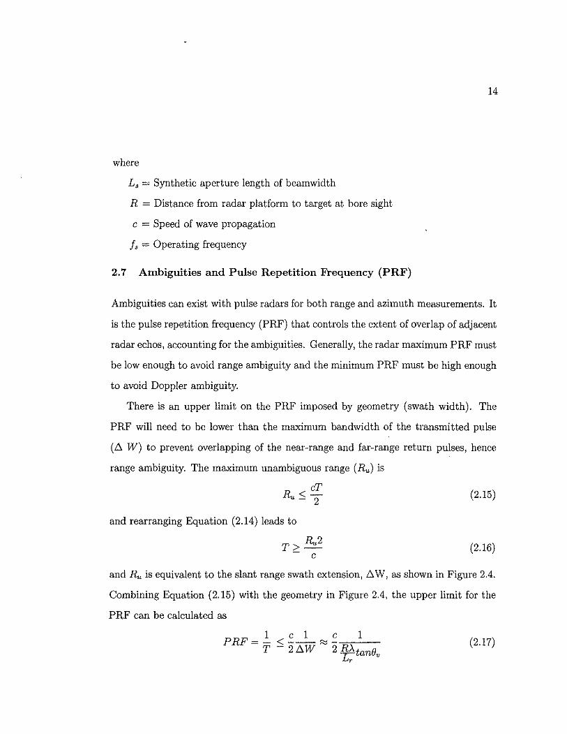
2.7 Ambiguities and Pulse Repetition Frequency (PRF)
14
Ambiguities can exist with pulse radars for both range and azimuth measurements. It
is the pulse repetition frequency (PRF) that controls the extent of overlap of adjacent
radar echos, accounting for the ambiguities. Generally, the radar maximum PRF must
be low enough to avoid range ambiguity and the minimum PRF must be high enough
to avoid Doppler ambiguity.
There is an upper limit on the PRF imposed by geometry (swath width). The
PRF will need to be lower than the maximum bandwidth of the transmitted pulse
(,6. W) to prevent overlapping of the near-range and far-range return pulses, hence
range ambiguity. The maximum unambiguous range (Ru) is
o < cT ""u - 2
and rearranging Equation (2.14) leads to
T> Ru2 - c
(2.15)
(2.16)
and Ru is equivalent to the slant range swath extension, .6. W, as shown in Figure 2.4.
Combining Equation (2.15) with the geometry in Figure 2.4, the upper limit for the
PRF can be calculated as
1 c 1 c 1 PRF = T :s: -2-A W- "" 2 R'
L> -t;tanBv (2.17)

Figure 2.4: Slant range swath geometT1J to discern range ambiguity
where
R = Line of sight range from antenna to target
b.W = Transmitted pulse bandwidth
L / = Length of antenna along the range dimension
Bv = antenna vertical beamwidth
Bi = incidence angle
15
On the other hand, Equation (2.11) pointed out that the Doppler bandwidth is
constrained [Ulaby, et aI., 1981} by the antenna beamwidth as it is repeated here to
be
(2.18)
The radar PRF must be chosen to be greater than this as to limit aliasing and avoid
Doppler (azimuth) ambiguity, thereby yielding an overall expression for the lower
limit of the PRF given by
(2.19)

16
2.8 Linear Frequency Modulation (LFM)
Most SAR systems use some form of linear frequency modulation (LFM) to achieve
a high range resolution. Actually, this design is more interested in the chirp radar
signal, which uses a combination of a pulse and FM signals. However, the area
where the chirp and the LFM generally differentiates themselves in that the chirp
requires a matched filter to de-chirp the echo signal for processing (thereby achieving
maximum SNR), whereas the LFM simply uses the heterodyne process to prepare
the echo for interpretation by the DSP. This thesis will use the terms; chirp and
LFM, interchangeably since the design will use the process of implementing a psuedo
matched filter by shifting the echo signal.
The general principle of the transmitted chirp waveform is illustrated in Figure 2.5.
T H-----PRI----.....
(a) Frequency-Time Plot
A
(b) Amplitude-Time Plot
Figure 2.5: Linear Frequency Modulation (LFM) waveform
The SAR design synthesizes a stepped-chirp FM pulsed wave as it is transmitted
waveform. Part (a) of Figure 2.5 shows the instantaneous frequency transmitted, that
is, the FM begins with an upward sweep for a period of ~, followed by a downward
sweep for the remainder of the pulse width. The transmitted waveform shown in
Part (b) is modulated in frequency from a lower frequency to a higher frequency and
return to the lower frequency in the time duration of the pulse width (T).

17
One of the remarkable aspects of this SAR design lies with the simple synthesis
of the chirp waveform. A software programmable AID card supplies a linear voltage
signal to an RF yeO, which then produces the chirp FM waveform. A computer
timing card manages the overall timing and control of the system, to include the
creation of the synthesized wave.

3.1 Design Consideration
Chapter 3
System Design
18
This chapter provides a simplified system design for a rudimentary, low-altitude, low
velocity synthetic aperture radar. This thesis provides for a baseline, or rather, an
introductory step-evolution towards this goal. The goal of this project is to design
and develop a high range resolution (HRR) radar with system parameters that can
be expanded into an X-band SAR system in the future. The HRR radar is able to
detect various simultaneous targets (trihedrals) and also be able to distinguish these
targets in the slant-range configuration. Some important design issues that have been
considered include:
(a) 'Transmit Waveform
In radar remote sensing, there are two widely used configurations, namely the
pulse and FM-CW (frequency modulated continuous wave) schemes. The finite
duration of the pulse permits range discrimination for the pulse radar at an
increased average power than that of the CW signal. However, a third scheme
combines the pulse and the FM: this is the chirp waveform. The duration of the
chirp waveform is longer than would be required for the range discrimination,
but the energy in the pulse is the same as it would be for the equivalent short
pulse. This permits the same maximum range that could be achieved with a high

19
peak-power short pulse. Figure 3.1 shows the transmit waveform used in this
system.
F t)
PRI=25ms
Figure 3.1: Synthesized transmitted chirp waveform characteristics.
The pulse duration width, Tis 172.4 f-ts; up-ramp of 86.4 11,8 (216 x 200 ns x 2 =
86.4 f-ts), plus the down-ramp of 215 Its (215 x 200 ns x 2 = 86.0 Its). The pulse
repetition interval (PRI) is 2.5 ms (or equivalently, PRF = 400 Hz). The need
to start the chirp 2.0 ms into the period is to ensure that the returns arrive only
from the footprint illuminated on the ground at the specified aircraft altitude and
incidence angle.
(b) Operating Frequency
The operating frequency of any radar system is primarily based on the function
the system is to accomplish. At this preliminary stage of this SAR system,
the functional goal is to simply distinguish between simultaneous slant-range
targets at a determined resolution. However, ultimately this SAR will serve as an
airborne-platform, remote-sensing radar for underlying terrain parameters. With
this function in mind, the radar system is operated in the X-band range with
a frequency band between 9.8 GHz to 10.2 GHz and a bandwidth of 400 MHz.
The extent of penetration into vegetation depends upon the moisture content
and density of the vegetation as well as upon the wavelength of the signal. At
X-band, the wavelength is approximately 3 cm in length and roughly on the

20
same scale of the crop sterns or vegetation it will be measuring. Since X-band
signals do not penetrate into the tree canopy, it will be able to yield information
about the upper layers of the vegetation and superficial layers of certain types
of ground cover. Parameters that are of interest include: leaf area index (LAI),
above ground biomass, and tree height.
(c) Operating Platform
To simulate the low altitude (an indication of grazing angle), low-velocity (an
indication of Doppler) effects of the SAR, the radar system is mounted on a
telescopic boom-mounted van. The altitude, grazing angle and velocity param
eters considered by the system are restricted to the limitations imposed by this
platform. Figure 3.2 shows the ground testing geometry.
... ................... ...... ~ .. ,., .. , .................... .. Grazing angle
.. ..... Downrange
Figure 3.2: Overview of radar platform in relation to target
(d) Calibration
Calibration is needed to remove measurement errors due to inherent instrumenta-
tion measurements and measurement techniques. To remove the internal system
variations such as the ambient temperature fluctuations, phase change due to ca
ble flex/length mismatches and gain drifts in the amplifiers. The DSP section will
address and correct for these calibration errors during processing. Other errors,
such as distortions caused by active components and antennas, will be adjusted

21
for or removed when comparing the received echoes with a measured response of
a known calibration target (i. e. a conducting sphere).
(e) Signal Processor
The processing of the return signal into an acceptable image is arguably one of
the more complex aspects of the SAR design, following the signal generation.
However, the DSP of the received echo is beyond the scope of this research and
will not be considered in this thesis.
A summary of the system requirements listed in Table 3.1 are used as basic guide-
lines to select suitable system parameters.
Table 3.1: Summary of Design Considerations
System Parameter Design Considerations
System configuration Stepped-chirp FM synthesized wavefonn
Operating frequency X-Band
Calibration htternal and external measurement errors addressed in signal processing
Operating platfonn A mobile boom-mounted van
Signal processor PC-based system
3.1.1 Design Parameters
. In Section 2.2, the radar equation derived shows how the received power is related
to radar and target parameters of the system. The equation is duplicated here for
convenience and is used to examine the individual parameters of the system.
(3.1)

22
The waveform generation uses an X-band veo that has a linear response in the
required 10 GHz range and the average transmit power of 12.6 mW (+11 dBm).
The operating frequency is at X-band with a wavelength (,x) of 3 cm for the reasons
described in Section3.1(b). The RF amplifier amplifies the transmitted signal (P,) by
+29 dBm to +40 dBm. The radar cross section (ReS) is proportionally related to the
amount of reflected power diverted back towards the receiver from the illuminated
area. A value of 10 dB will be used for the average ReS fluctuations (0'): this
value is based on the several factors, such as terrain cover, angle of incidence, target
composition, etc. [Skolnik, 2001]. The system uses two separate microstrip antenna
arrays, each with virtually identical gains of 25 dBi. For a ground-based system
operating at a boom-mounted van platform, the radar-to-target range (R) can vary
between 20 meters to 100 meters.
Noise is a major factor limiting overall system performance. The SAR system
design has a low noise amplifier (LNA) as the front end of the receiver. A consequence
based on how the overall noise figure affects the system performance is considered.
A complete measure of the noise sensitivity of the receiver takes into account the
noise figures and gains of the cascaded networks; i. e. the LNA, the mixer stage, the
IF amplifier stage and any losses in the RF transmission line. The receiver noise is
calculated as
(3.2)
with the Fx's and the Gx's representing the individual cascaded network losses or gains
within the receiver, respectively. Finally, the remaining parameters in Equation (3.1)
are considered to be constants and are system independent.
Table 3.2 summarizes the significant design parameters of the X-band SAR system.

23
Table 3.2: SAR System Design Parameters
System Parameter Selected Value
System configuration Stepped-chirp FM syuthesized wavefonn
Opemting wavelength, ). 3 em (X-band)
Transmit power, Pt 20 dBm - attenuated from original lOW (or 40 dBm)
Received power, Pr -35.5 dBm (min muge), -63.5 dBm (max muge)
Measurement range, R 20 meters (min) to 100 meters (max)
Avemge ReS, (J 10 dB
LNA noise figure, F Ii 3dB
IF filter (center frequency) 30 MHz
IF bandwidth, B 7 MHz
Antenna gain, G 25 dBi
Thermal noise -133.8 dBm
Separating Equation (3.1) into the noise and the received power considerations to
realize the approximate signal to noise ratio results in:
Noise power:
Received power: R=20m R = 100m
Therefore, the signal-to-noise ratio (SNR) is computed as
SNR= Pr = { 67.5 dB Pn 39.5 dBm
for near reflectors for far reflectors
(3.3)

24
3.2 System Description
The X-band SAR design is based on a low-cost approach relying on recent advance
ment in digital and RF technology to develop, what is historically a large and expen-
sive instrument, into a compact and relatively inexpensive testing instrument.
In addition to the previously stated system design parameters, the SAR design
is subjected to the constraints of being built on a low budget and having a minimal
impact on the delivery platform (airplane, boom-mount van, etc.). These constraints
combined, dictate many of the design decisions employed into the SAR.
The schematic of the integrated X-band SAR system is shown in Figure 3.3. In
general, the design may be subdivided into four major sections:
• Signal Generation
• RF section
• Receiver section
• Data Acquisition
·································s;~~·~Ch~;;;·G;~~~~~i~~·11'" ................................. ········ .. RF;s;~ii~;;··l
!
......................... l:: .. : ....... _
Receiver Section
...................................... .P.~.~.~~.~.~~~.~~.J
Figure 3.3: Top-level block schematic of BAR design.

25
3.2.1 Signal Generation Section
The signal waveform generation is perhaps the most vital and complex section within
the entire system design. The SAR operates by timing the two-way delay for a short
duration RF pulse, transmitted vertically downwards and to one side of the aircraft.
The required level of accuracy in range measurements (better than 4 m) calls for a
pulse length of a several nanoseconds; therefore, in order to reduce the RF power
requirements, a pulse compression (chirp) technique is used. The waveform can be
tied directly to the slant-range resolution of the system. Additionally, the PRF, pulse
width, bandwidth and the linearity of the veo output signal are vital to the SNR of
system.
An ideal chirp waveform would have a perfect ramp function of frequency versus
time as depicted in Figure 3.4 ( a) where at any time along the duration of the trans
mitted pulse (T) lies a unique frequency (fTX - fRx) = !IF, called the intermediate
frequency.
F(') F(')
f.u Tx R. ... f ....... . ~ ... "." Tx RJ<
i B = (f.u - f • .>
1 ~·~-L--------~--~·t
~T=t~ (a) (b)
Figure 3.4: (a) Ideal LFM Waveform. (b) Actual LFM Waveform.
The ideal LFM ramp could be generated by a very expensive and sizeable X-
band synthesizer. However, with the constraints imposed on the design of low-cost
and having a small footprint, a solution of generating the waveform using a D / A
computer card and an X-band veo was implemented. In Figure 3.4 (b), the actual

26
waveform generated from the D / A-veo combination illustrates a stair-step ramp. It
is important that each vertical step length be reduced as to approach a linear slope.
The stair-step emerges as a result of the limitations of the generation rate (Rg) and
the output bit-resolution of the D / A card, and the inherent settling time of the yeo.
The range resolution in Figure 3.4(a) is calculated as
c 0,. = 2B
when the LFM has a linear slope, or the alternative equation
CT 0,.="2
(3.4)
(3.5)
can be used when the solving for a stair-step slope as in Figure 3.4 (b). In Fig
ure 3.4 (a), the pulse duration of chirp is equal to the reciprocal of the bandwidth,
i.e. T = 1/ B (or equivalently; l' = 1/ B). However, in Figure 3.4 (b), the pulse width
l' is no longer equal to the reciprocal of the bandwidth but is now equal to the width
of horizontal step in the stair-stepped LFM (T of t and l' of 1/ B).
Table 3.3 lists the range resolution results from both equations.
Table 3.3: Range Resolutions
Equation 3.5 (stair-step slope)
Rg T Range
(Megasample/sec) (~= I/Rg) Resolution
80 Ms/s 12.5 ns 1.88 meters
40 Msis 25.0 ns 3.75 meters
Equation 3.4 (LFM slope)
Bandwidth Pulse Width Range
(B) (T) Resolution
400 MHz 2.5 ns 0.375 meter

27
Since the HRR system design will serve as the hardware platform for the X-band
airborne SAR, certain compromises must be made at this stage between incorpo
rating the airborne-platform SAR parameters (e.g. increased range-to-target) versus
attempting to design for the greatest range resolution of a ground-based system. For
an airborne-platform, the designated range-to-target is 750 meters, which has the
optimal pulse duration of the chirp of 102.3875 /lS (as explained in the Receiver
Section of this document). The following table establishes the relationship between
the output bit resolution of the D / A, the generation rate of the D / A card and the
associated pulse duration.
Table 3.4: D/A Bit-Resolution vs. Pulse Duration
DIA Bit Generation Rate Pulse Duration Resolution (Rl!:) (T)
SAR design 216 bits 5 Ms/s 172.8/-1s
Current design 216 bits 80 Ms/s 1O.8/-1s
With extender circuit 4096 bits 80 Ms/s 51.2 /-Is
The original design of the waveform generation was specifically designed to meet
the parameter criterion for an airborne platform SAR. The design did not take ad
vantage of the full output range of the D / A and was restricted to only 216 bits. This
restriction of 216 bits required the pulse duration time to be significantly large to
accommodate the greater range-to- target distance; therefore a low generation rate of
5 MHz is required. The 216-bit limitation results from difference in the bit represen
tation of the output voltage from the D/A component (Le. D/A bit 800 = 6.01 V =
10.2 GHz and D/A bit 584 = 6.99 V = 9.8 GHz; 800 - 584 = 216 bits). However, since
the HRR radar is tested on the ground and at a considerable shorter range-to-target
distance, a higher generation rate of 80 MHz can be considered. This higher rate will

28
provide a better range resolution for a shorter range. Again, this current design is
still limited to the 216-bit limitation as explained with the SAR design. However, to
gain a much finer range resolution with the existing hardware, an analog" extender"
circuit (schematic in Appendix A.3) is included into this design and thereby taking
advantage of the entire 4096-bit (216 bits = 4096) range from the output of the D/ A
card as illustrated in Figure 3.5.
-10 V
6.99 V
6.01 V
ov
·IOY
t. 6it584
t Bi(81)O
216uscnblebits
4096 available bilS
(a) Original DfA output resolution
+IOV
,v
-JOY
i I 1
4096 U:leable bit~
(b) Df A output resolution witb improvement with added circuitry
Figure 3.5: D / A Output Bit Resolution.
The greater number of bits representing the same voltage range (6.01 V to 6.99 V)
of the D / A output would equate to a smaller voltage increment feeding the varactor
inside the yeo. The 4096-bit analog output of the D/A card is combined with the
precision steady state analog voltage of the extender digital circuitry, to provide the
required input to the yeo. The input analog feed to the veo will provide a very
precisely correlated voltage-input to frequency-output synthesizing the desired LFM
waveform. The frequency on the veo is tuned (modulated) by varying the applied
voltage from the D / A-extender circuit combination. The tuning characteristics of
the veo are provided in Appendix A.I. The extender analog circuit addresses two
separate problems: (a) the settling time parameter of the veo is excessively large
(~150 nsec), and (b) the output bit resolution of the D/A card was restricted to 216
bits. By extending the output bit resolution of the D / A card, the incremental analog

29
voltage input to the veo was dramatically reduced, thereby preventing the internal
varactor of the VCO from fully charging and discharging. This charging/discharging
corresponds directly to the settling time of the yeo. Changing the analog input
voltage to the VCO to smaller increments changes the charge level on the varactor
only minimally and in turn, improves the recovery time of the veo considerably.
Increasing the recovery time of the varactor reduces the settling time of the veo and
provides for a more linear ramp to the waveform. If more time and resources were
available to improve on the analog design, it is believed a greater gain would result
in the range resolution from such a small contribution. It will be left up to the next
generation of hardware to improve on this circuit.
Figure 3.6 summarizes the synthesized LFM -chirp waveform;
F(t)
10.2 GHt·· ........................ .
ffi (6.01 Vl . . . • + +.
9.8 GHz-jJ---------i----------+(6.99 V)
~- 216sleps --";II:+--------- 215sleps , l'4 , .... -...... -----.... --. T = 10.78 JlS
Figure 3.6: Waveform parameters.
3.2.2 Radio Frequency (RF) Section
The RF section consists of the aforementioned signal generated section, the power
divider and the high power RF amplifier. Setting aside the signal generation, the RF
section is fairly straightforward. The power divider receives the generated waveform,

30
where the signal is reduced by 3 dB at each exit port. The signal at one port is used
as a local oscillator to be mixed with the received echo return. The signal at the
remaining port is passed onto the RF amplifier where the power level is increased
by 29 dB. Although the maximum RF amplifier gain is rated at +40 dB, an ll-dB
attenuator at the output port limits the amplifier gain to +29 dBm. This prevents
saturation of the receiver LNA for shorter-range operation. The full amplification
of the RF amplifier will be required in the airborne SAR configuration, where the
range to target is increased dramatically. After the power level of the signal has been
amplified by the RF amplifier, the synthesized LFM chirp signal is then coupled into
free space via the transmitting antenna.
3.2.3 Receiver Section
The main function of the receiver section (or IF section) is to filter and amplify the
return echo signal. The receiver antenna receives the re-radiated echo returns from
the target, which are at a considerable lower power level than when the signal left
the transmitter. The LNA amplifies the return signal by 30 dB to elevate the weak
signal to required SNR levels. At this stage, the signal is at RF and is rather difficult
and expensive to manipulate. The high frequency signal is down-converted into an
intermediate frequency (IF) signal by a mixing process. The single side band (SSB)
mixer, a down-converter, outputs the difference in frequency between the copy of the
transmitted signal and the received echo return: IfLO - fRFI = fIF.
Referring to the radar Equation (2.5), the received power decreases at a rate
proportional to R4, which means that if the range-to-target is doubled, the received
power will decrease by a factor of 16. As the range increases, the maximum received
power decreases but the minimum detectable power level remains the same. This
is due to the fact that the thermal noise level is independent of range. Therefore,

31
the overall effect is the decrease in the system dynamic range. This decrease in the
system dynamic range can be avoided by employing a variable gain amplifier in the
IF stage. The AGe (automatic gain control) of the IF amplifier is adjusted via an
external potentiometer, to accommodate the dynamic range the radar. The center
frequency of the IF amplifier is at 30 MHz with a bandwidth of 10 MHz. The noise
figure of this amplifier is 4 dB, which is still greater than that of the front-end LNA,
and although the amplifier has the maximum gain of 70 dB, minimum gain will be
used during ground testing. The last stage of the IF section is band pass filter (BPF).
The BPF is inserted after the IF amplifier to reject any unwanted signal outside the
passband (30 MHz ± 3.5 MHz). The IF frequency is directly proportional to the
range, as can be seen the following equation
!IF = 2BR cT
(3.6)
where B is the system bandwidth, T is the pulse duration time, c is the speed of light
and R is the range-to-target. On the airborne SAR platform, the estimated range from
radar to target is 1000 m, the pulse duration is 102.4 j.tS and the system bandwidth
is 400 MHz. Substituting these values for the parameters in Equation 3.6 leads to
the IF frequency of 30 MHz. To determine the bandwidth of the IF frequency, which
directly determines the 3-dB cutoff requirement of the BPF, the following equation
is used
f,.!IF = 2Bf,.W cT
(3.7)
where f,.W is the swath width on the ground as determined in Equation (2.21). In
the SAR configuration, the swath width is 100 meters, which would bring the IF
bandwidth to 7 MHz. The output of the band pass filter is then fed to the data
acquisition section for further processing.

DESIGN AND DEVELOPMENT OF A LOW-COST
HIGH RANGE RESOLUTION X-BAND RADAR
by
Paul Cantu
A THESIS
Presented to the Faculty of
The Graduate College at the University of Nebraska
In Partial Fulfillment of Requirements
For the Degree of Master of Science
Major: Electrical Engineering
Under the Supervision of Professor Ram M. Narayanan
Lincoln, Nebraska
August, 2003

DESIGN AND DEVELOPMENT OF A LOW-COST HIGH RANGE RESOLUTION X-BAND RADAR
Paul C. Cantu, M.S.
University of Nebraska, 2003
Advisor: Ram M. Narayanan
Synthetic Aperture Radar (SAR) is one of the main tools for microwave remote sens-
ing because of its multi-dimensional high resolution characteristics and the capabil-
ity to operate in nearly all weather conditions, day and night. The University of
Nebraska-Lincoln (UNL) initiated the design and development of a low-cost airborne
SAR in January 2001 to support our Airborne Remote Sensing Program. The objec-
tives of this project are separated into various evolutionary stages. This thesis will
focus on the initial phase of design and construction of an X-band high range resolu-
tion radar (HRR) using basic RF /microwave and digital components. The following
stages will expand on the HRR design to achieve a functioning X-band airborne SAR
for the remote sensing of underlying vegetation parameters (tree height, leaf area
index, biomass content, etc.) from a low altitude platform from a range of 1000
meters. The SAR system is an X-band, stepped-chirp FM, single polarization radar
system. One of its unique features is that the signal generation consists of a timing-
controlled D / A converter and VCO arrangement to generate the step-chirp signal,
thereby allowing for less design complexity and a much lower overall system cost.

The individual block-segments of the SAR include a stepped-chirp FM waveform
synthesizer, transmission and receive paths, antennas, quadrature detection and im
age signal processing. The system underwent rigorous in house laboratory testing and
subsequent outdoor field-testing from a van-mounted boom where preliminary HRR
one-dimensional images were obtained. It is anticipated that the following progres
sion of development for this HRR system will be to use this design as a basis towards
fully coherent, data acquisition from an airborne platform.

ii
Acknowledgments
I would like to acknowledge the following for help, encouragement, and support during
the preparation of this thesis. First, I thank God for giving me the endurance and
perseverance to complete this work. I could not have completed this work without
the continuous support of my wife and two children. The support and encouragement
of all my family members and friends are greatly appreciated.
Extended thanks for financial support form;
• NSF (for funding the airplane)
• NASA EPSCoR Program (for funding this research)
This project is supported through a grant from the NASA EPSCoR program
through the Nebraska Space Grant Consortium.
Special thanks to my committee members Dr. Donald C. Rundquist and Dr.
Robert D. Palmer for their support and contributions.
Extra-Special thanks to my team member; Mr. Guangdong Pan for his never
ending assistance in signal processing and field work. Without his help, the HRR
would simply be a heap of inert hardware. Thank you MR. Pan for putting up with
my impatience and I wish the best for you in all your endeavors. Additional gratitude
to team members; Mr. Xiaojian Xu for the initial design concept and Ms. Sujin Kim
for picking up where Mr. Pan left off.

iii
I would like to acknowledge two special lab-mates; Mr. Brian" da man" Corner
and Mr. Cihan Kumru, both of whom contributed no significant knowledge, but
without their levity, humor and friendship made coming to the lab bearable.
I would like to express my utmost gratitude and greatest appreciation to Dr. Ram
M. Narayanan for allowing me to be one of his coveted research assistants and for
being my advisor.

Abstract ..... .
Acknowledgments
Contents ....
List of Figures
List of Tables .
1
2
Introduction.
1.1 Motivations
1.2 Scope of the Thesis
Review of Radar Theory
2.1 Radar Fundamentals
2.2 The Radar Equation.
2.3 SAR Principles . .
2.4 Range Resolution
2.5 Azimuth Resolution
2.6 Doppler Bandwidth
Contents
2.7 Ambiguities and Pulse Repetition Frequency (PRF)
2.8 Linear Frequency Modulation (LFM)
3 System Design ....... .
3.1 Design Consideration
3.1.1 Design Parameters .
iv
ii
iv
vii
x
1
1
2
4
4
5
7
9
10
12
14
16
18
18
21

4
3.2 System Description . . . . . . . .
3.2.1 Signal Generation Section
3.2.2 Radio Frequency (RF) Section
3.2.3 Receiver Section
3.2.4 Antenna Section
3.2.5 Data Acquisition Section .
Analysis and Results . . . . . . .
v
24
25
29
30
32
33
35
4.1 Laboratory Test Results 35
4.1.1 IF Gain-Saturation Problem. 36
4.1.1.1 LFM Transmitted Signal and Power Spec-
trum (Saturation UUT). . . . . . . 36
4.1.1.2 Saturation UUT - Include The IF BPF 40
4.1.1.3 Saturation UUT - Include The IF Amplifier 42
4.1.1.4 Saturation UUT - Include The LNA And IF
Amplifier ................ 44
4.1.2 LOW-FREQUENCY Interference Problem 46
4.1.2.1 Identifying Low Frequency (Low Frequency
UUT) ......................... ~
4.1.2.2 Low Frequency UUT Changing the AID Sam
pling Rate . . . . . . . . . . . . . . . . . . . . .. 50
4.1.2.3 Low Frequency UUT - Including the IF BPF 51
4.1.2.4 Low Frequency UUT - Including the RF Am-
plifier . . . . . . . . . . . . . . . . . . . . . . . .. 54
4.1.2.5 Low Frequency UUT - Normal System Con-
figuration . . . . . . . .
4.1.3 Laboratory Testing Conclusions
55
59

5
4.2 HRR Radar Data Processing
4.2.1 Data Structure .....
4.2.1.1 Generating Pulse
4.2.1.2 Acquiring Data.
4.3 Field Test Results . . . . . . . .
4.3.1 HRR Radar Profiling Results.
4.3.1.1 Reference Target Range Results
4.3.1.2 4 meter range results
4.3.1.3 3 meter range results
4.3.1.4 2 meter range results
4.3.1.5 Truck range results
4.4 Concluding Analysis.
Conclusions . . . . . . . .
5.1 Summary of Work
5.2 Recommendations for Future Work
Bibliography
Appendix ..
A.l VCO Data Sheets
A.2 X-band Antenna Data Sheets
A.3 Analog Extender Circuit . . . .
vi
60
60
61
62
64
64
68
69
70
71
72
73
77
77
78
79
80
80
81
83

List of Figures
2.1 Footprint Definition. . . . . . . . . . . . . . . . . . .
2.2 Definition of Range Resolution Between Two Points .
2.3 Doppler spread geometry of a synthetic aperture . . .
2.4 Slant range swath geometry to discern range ambiguity
2.5 Linear Frequency Modulation (LFM) waveform . ....
3.1 Synthesized transmitted chirp waveform characteristics.
3.2 Overview of radar platform in relation to target
3.3 Top-level block schematic of SAR design. . . . .
3.4 (a) Ideal LFM Waveform. (b) Actual LFM Waveform.
3.5 D / A Output Bit Resolution.
3.6 Waveform parameters . ...
Vll
8
9
13
15
16
19
20
24
25
28
29
4.1 UUT- Testing LFM, Transmit, Receive and Data Acquisition. 37
4.2 VCO-50dB-LNA-9.8GHz-Mixer-200m V. 38
4.3 VCO-70dB-LNA-9.8GHz-Mixer-50m V. 39
4.4 UUT- Testing IF passband. . . . . . . . 40
4.5 VCO-50dB-LNA-9. 79GHz-Mixer-BPF-l OOm V. 41
4.6 UUT-Testing IF Amplifier and AGC Saturation Level. . 42
4.7 VCO-50 dB-LNA-9.78GHz-Mixer-IF-l0v (Gain 70 dB). . 43
4.8 VCO-50dB-LNA-9. 78GHz-Mixer-IF-A GC2v-l Ov{Gain < 70dB). 44

viii
4.9 UUT-Testing Complete System Design. . . . . . . . . . . . . . . 45
4.10 VCO-50dB-9.78GHz-Mixer-IF-AGC2v-BPF-l0v(Gain < 70 dB) 46
4.11 UUT- Testing the Low Frequency System Component. 47
4.12 VCO-BW40-PD-Mixer-2V. . . 48
4.13 VCO-BW40-PD-Mixer-20m V. 48
4.14 VCO-BW40-PD-Mixer-20m V. 50
4.15 VCO-BW40-PD-Mixer-500m V-Sampling Rate 500 MHz. 51
4.16 UUT- Filtering Out the Low-Frequency Effect. 52
4.17 VCO-BW40-PD-Mixer-BPF-50m V. . 53
4.18 VCO-BW400-PD-Mixer-BPF-50m V. 53
4.19 UUT Testing the Effect of the RF Amplifier. 54
4.20 VCO-BW40-PD-RF-40dB-Mixer-200m V. . 55
4.21 Testing Normal System Configuration. .. 56
4.22 VCO-B W400-PD-50dB-LNA-MIXER-IF(A GC3v)-BPF-2v. 56
4.23 VCO-B W400-PD-50dB-LNA-MIXER-IF(A GC3v)-BPF-lv. 57
4.24 VCO-B W400-PD-50dB-LNA-MIXER-IF(A GC3v)-BPF-500mv. . 57
4.25 VCO-BW400-PD-50dB-LNA-MIXER-IF(AGC3v)-BPF-200mv.. 58
4.26 Parameters of the LFM Chirp waveform. . . . . . . 61
4.27 Point Data Structure of the Transmitted Waveform. 62
4.28 Sampled Data Points from received waveform. 63
4.29 Target arrangement profile. . 65
4.30 Secondary target offset. . . . 66
4.31 A single Trihedral target at 20 meters down range (Reference Target.) 68
4.32 Reference Target at 20 meters and Secondary Target at 24 meters. 69
4.33 Reference Target at 20 meters and Secondary Target at 23 meters. 70
4.34 Reference Target at 20 meters and Secondary Target at 22 meters. 71

ix
4.35 Reference Target at 20 meters and Truck Target at 25 meters. 73
4.36 VCO Linearity Effects. . . . . . . . . . . . . . . . . . . . . . . 76
A.1 VCO tuning characteristics.
A.2 Antenna: E-Plane radiation pattern.
A.3 Antenna: H-Plane radiation pattern.
A.4 Antenna: Return-Loss. . . .
A.5 Analog EXTENDER circuit.
80
81
81
82
83

x
List of Tables
3.1 Summary of Design Considerations 21
3.2 SAR System Design Parameters. 23
3.3 Range Resolutions. . . ...... 26
3.4 D / A Bit-Resolution vs. Pulse Duration 27
3.5 Antenna Specifications ......... 32

1.1 Motivations
Chapter 1
Introduction
1
Monitoring the status and condition of the earth's terrain, such as vegetation fields,
forests and soil surfaces is of primary importance to the understanding and the pro
tection of the environment, as well as for natural resource management. It has been
recognized that the use of microwaves in remote sensing is a suitable approach as
microwave signals are able to penetrate cloud and vegetation cover and can operate
independent of solar illumination. Moreover, microwaves have the ability to pen
etrate more deeply into vegetation compared to optical signals. In general, longer
wavelengths penetrate vegetation much better than shorter wavelengths .. Currently,
there exist operational C-band and L-band systems operating in the 5 GHz and 1
GHz frequency bands, respectively, that are routinely used for sea surface and soil
moisture remote sensing. However, higher frequencies such as X-band (10 GHz) are
used for radar systems where the size of the antenna constitutes a physical limitation;
this becomes especially important when considering an airborne platform. The main
thrust in developing the X-band Synthetic Aperture Radar (SAR) is to provide a
light-weight, low-cost system to ultimately operate from an airborne platform. The
fact that the system operates in the X-band microwave range will allow for smaller RF
(radio frequency) components and antennas, relative to C-band and L-band, making

2
it ideal for airborne operations. The system design is one which is easy to maintain
and operate, and capable of quick turn-around in data acquisition.
Ultimately, X-band SAR will provide remote sensing of underlying terrain param
eters (tree height, soil moisture, biomass content, etc.) from an airborne platform;
however, there are several evolutionary steps needed towards accomplishing this goal.
This thesis will focus on the design and construction of the X-band high range res
olution (HRR) radar, which will be the core hardware design to the airborne SAR
system. The HRR radar will be tested and validated using ground-based tests from
a mobile boom-mounted van.
1.2 Scope of the Thesis
In this thesis project, a ground-based HRR radar system has been designed, con
structed and tested. This system is mounted on a mobile, van boom-arm during the
testing phase and validation phases. There are three objectives identified for this
project:
i. To design, construct and test a HRR radar system
The system design will be simple and straight forward. Simple, light
weight, compact, and low-cost design are the overall top-level requirements.
ii. To validate the H RR radar resolution
The HRR will produce a ground range resolution better than 4 meters.
iii. To use this technology as a basis towards the next evolution stage,
i.e., graduating this HRR radar system to an airborne SAR platform
The experience gained in this project will be used for future evolutions
towards an airborne platform SAR system.

3
This thesis reports on the design, development and testing results of the HRR radar
system. Chapter 2 will review radru' fundamentals, especially as they relate towards
the design of a synthetic aperture radar system using the HRR radar as the sys
tem hardware. In particular, the concept of the stepped-chirp signal generation is
highlighted.
A detailed description of the system design and its operation is presented in Chap
ter 3. In general, the construction of the SAR can be subdivided into five parts. These
include (a) the signal generation, (b) the radio frequency (RF) section, (c) the an
tennas, (d) the receiver section and (e) the data acquisition section. The HRR is a
quasi-monostatic radar, where a dual antenna system, in close relation to each other,
is employed in this design. This design configuration will eliminate the problems
associated with transmit/receive isolation, to minimized design complexity and the
potential to expand the system for interferometric applications. The RF section is
constructed from individual RF components. These include the use of a power split
ter, band pass filter and RF amplifier. The main function of the receiver section is to
filter and amplify the intermediate frequency signals received from the mixer output.
The pre-processed signals are then converted into digital data by the data acquisition
section, which includes an analog-to-digital (A/D) computer card, computer software
and the computer storage. Analysis and processing of the data can be performed
virtually in real-time while still gathering data on the aircraft or in the field.
Several radar cross section measurements have been carried out to verify the
operation of the SAR system. These include the measurements of standard targets
such as trihedrals of differing sizes at various downrange distances. The analysis,
results and observations are presented in Chapter 4.
Finally, Chapter 5 will conclude with a summary of work performed and future
recommendations for this X-band high-resolution radar.

4
Chapter 2
Review of Radar Theory
2.1 Radar Fundamentals
The term "radar" stands for RAdio Dectection And Ranging, This term was coined in
the early 1950s, at a time when detection of ships and determination of their ranges
were its primary purpose. However, after the proliferation of high speed computing,
digital processing and other advances, radar has graduated beyond simple detection
and ranging of targets, and is used in a wide range of applications for the military,
air traffic control, police departments and remote sensing, to mention a short list.
Generally, remote sensing refers to the process of recording/ observing/ perceiving
(sensing) objects or events at far away (remote) places. In remote sensing, the sensors
are not in direct physical contact with the objects or events being observed. The
technique requires an electromagnetic wave, of suitable characteristics, to travel from
the objects/events to the sensors through the atmospheric medium. The choice of
electromagnetic radiation wavelength (or frequency) depends upon the specific remote
sensing application.
Synthetic aperture radar is basically a method of ground mapping and imaging
that uses computer processing to sharpen the azimuthal resolution over what can
be achieved by a conventional antenna. This technique first appeared in the early
1950s, but did not reach a high state of development for almost 30 more years. With
the introduction of high-speed digital processing and other advances, SAR is rapidly
emerging as a powerful remote sensing tool (Ulaby, et al.,1981).

5
2.2 The Radar Equation
In microwave remote sensing, the distinction between different ground targets being
sensed is primarily caused by the difference in the signal strength received by the
radar. Therefore, it is understood the received signal strength is the most important
measurement in remote sensing. In the simplest case, the radar equation can be
stated verbally as suggested by [Ulaby et.al,1981J:
!power '1 t'eceive~ =
rpowel' pel' uni] >1< rEffecti~e scattermg] * larea at target l~"'ea oj the target
ISpreading loss Of] * !Effective antenna] ~'adiated signal ~'eceiving area
where the power at the receiver is the energy scattered back from the target (i.e.
backscatter). The power per unit area at the target is the amount of energy inter
cepted by the ground target as a result of its physical characteristics. The effective
scattering at the target represents the re-radiation of energy in all directions from
the point source (ground target), to include that fraction of power received at the
receiver. The spreading loss of radiated signal stems from the nature of the radiated
power from the point source spreading out in all directions in the area of a sphere of
radius R. The further away from the point source, or the greater the radius R, the
less power received at the receiving antenna. The actual size of the receiving antenna
will also affect the total power received.
The phonetic equation can be used to assist in deriving the fundamental radar
equation as follows:
(2.1)

Pr = Power received
P, = Power transmitted
Gt = Gain of the transmitting antenna
(J = Radar cross section
Gt = Gain of the transmitting antenna
Gt = Gain of the transmitting antenna
This equation can be broken down further for clarification:
(J
(1) = (2) * (3) * (4) * (5) * (6) * (7)
6
(2.2)
The power received (1) by the radar system Pr, is a function of a linear frequency
modulated chirp pulse of electromagnetic energy, Pt (2), that has been focused down
by the transmitting antenna to a beam width, so that the energy level increases
by a factor of Gt (3) over a spherically expanding wave (4). This focused energy
illuminates an area on the ground that has a radar cross section (ReS) of (5). The
backscattered power then radiates isotropically (or spherically) in all directions from
the point scatter (6). The receiving antenna area, Ar (7), intercepts a fraction of this
backscatter signal for processing.
Although the SAR sports a two-antenna design, both antennas are generally iden-
tical to each other in all characteristics, including gain, i.e. G = Gt = Gr. As per
[Ulaby, et al.,1983]' the relationship between the antenna directive gain and receiving
aperture area is:
or equivalently; G),2
Ar=--47r
(2.3)
(2.4)

7
where oX is the wavelength of the radar system. Substituting Equation (2.4) into
Equation (2.2) or (2.1) results in a modified radar equation:
(2.5)
There are several forms of this radar equation; however, one common form equates
the ratio of the returned signal power, S (or p,.), to the receiver noise power, N. The
noise figure of the receiver, FN , and the thermal noise power, kTB (k = Boltzman
constant, T = Temperature, B = Bandwidth), as well as the system and environ
mental losses, L, are integrated into Equation (2.6) to become the radar equation of
interest. The Signal-to-Noise (power) ratio at the receiver antenna port is
(2.6)
2.3 SAR Principles
SAR systems can produce maps (or images) of radar reflectivity versus range and
azimuth, typically in the form of a two-dimensional (2-D) image. One dimension in
the image is called range and is a measure of the "line-of-sight" distance from the
radar to the target. Range measurement and resolution are determined by precisely
measuring the time from transmission of a pulse to receiving the echo from a target.
Fine range resolution can be accomplished through pulse compression techniques,
such as in this design: linear frequency modulation (LFM) chirp.
The other dimension is called azimuth (cross-range) and is perpendicular to range.
It is the ability of the SAR to produce a relatively fine azimuth resolution which
differentiates it from other radars. To obtain fine azimuth resolution, a physically
large antenna is needed to focus the transmitted and received energy into a sharp
beam. The sharpness of the beam defines the azimuth resolution. Fine azimuth

8
resolution is enhanced by taking advantage of the radar motion in order to synthesize
a larger antenna aperture, which exploits the Doppler effect. The distance the radar
platform travels in synthesizing the antenna length is known as the synthetic aperture.
A narrow synthetic beamwidth results from the relatively long synthetic aperture,
which yields finer resolution than is possible from a smaller physical antenna.
The quality of SAR images is heavily dependent on the size of the map resolu
tion cell. The resolution cell is the area comprised of the range resolution by the
azimuth resolution. In the following subsections, the range and azimuth resolutions
are explained and calculated for this design.
R
63dB
~~ ............ ~.;t.--..... .-;-..... R .... -....... -] ....... : ......... K: J:~F:~ ;+- R *83dB "'sece~ . (swath width) i
Figure 2.1: Footprint Definition.
Figure 2.1 shows the geometry for the standard side looking SAR. As noted, the
intersection of the antenna beam with the ground defines a footprint. As the platform
moves, the footprint scans a swath on the ground, whose width is determined by the
antenna beamwidth, range and incidence angle. The antenna 3 dB beamwidth is
03dB, the range from the platform to the target is R, and the incidence angle is 0;.
Therefore, the size of the footprint painted on the ground is
RO 0 R03dB R)"
3dB sec ; = --0- = L 0 cos i vCOS i (range direction)

9
R(J3dB = ~~ (azimuth direction)
where Lv is the vertical length and Lh is the horizontal length of the physical antenna,
and A is the radar wavelength.
2.4 Range Resolution
Ground range resolution is defined as the minimum distance on the ground at which
two object points can be imaged separately, shown in Figure 2.3, as the distance oRg •
e, R",
, ,~ '/" , , , ,
, , . .'/ :8,
1'<""1
Figure 2.2: Definition of Range Resolution Between Two Points
Two individual point targets can be distinguished if the leading edge of the pulse
echo from the more distant point target arrives at the antenna later than the trailing
edge of the pulse echo from the nearer object, Thus, if their distances to the antenna
are different by at least half of the pulse length (product of the pulse width, t, and
the wave propagation speed, c), then the two objects are resolvable [Wehner, 1995].
Range resolution is determined primarily by the transmitted pulse bandwidth, i.e, a
narrower pulse yields a finer range resolution, Therefore the ground range resolution
oR =~ 8 2 (2,7)

10
oR = oRs = ~= c 9 sinei 2sinei 2Bsinei
(2.8)
where oRs is the slant resolution, Bi is the incident angle, T is the pulse length, t is
the pulse width, B is the frequency bandwidth of the transmitted radar pulse and c
is the speed of light.
The ground range resolution is infinite for a vertical look angle (ei = 0°) and
improves as the look angle is increased. Also, note that the ground range resolu-
tion is independent of the height of the radar platform. In order to achieve a fine
range resolution, the pulse width must be minimized, which is accomplished via the
frequency-modulated pulse (chirp) rather than resorting to using very short physical
pulses. This, in affect, will reduce the average transmitted power and increase the
operating bandwidth. Achieving fine range resolution while maintaining adequate
average transmitted power can be accomplished by using a pulse compression (i.e.
modulation) technique as described in Section 2.8.
2.5 Azimuth Resolution
The SAR system has a major advantage over the real-aperture side looking airborne
radar (SLAR) in that the resolution in the azimuth direction is independent of the
radar platform altitude or range distance to the target. SAR systems depend upon
two conditions; (1) the motion of the radar platform relative to a stationary target,
and (2) signal processing. Both of these conditions are used to synthesize an antenna
(aperture) that is much longer in length than the actual antenna hardware. Condi
tion (1) achieves this by taking advantage of the Doppler effect, and condition (2) by
achieving a much narrower beamwidth in the along-track direction than that attain
able with the real-aperture systems. Therefore, a larger synthetic aperture produces
a finer azimuth resolution.

11
The SAR system transmits the microwave pulses to the imaging area and the
echoes are received as "raw" SAR data, which are coherently recorded onto storage. It
is these recorded echoes, which generate a coarse (raw) microwave reflectance 'image'
of the illuminated ground area. The natural dimensions of this image are range and
azimuth. Whereas the range resolution of the raw image is dictated by the pulse
width (as described in Section 2.4), the 'raw' azimuth resolution is determined by
the azimuth extent of the antenna pattern footprint on the ground, the antenna size,
wavelength and the imaging geometry (SLAR properties). This 'raw' data in azimuth,
would exhibit an unacceptable image for this dimension. Subsequent image processing
of the 'raw' SAR data is required to dramatically improve the azimuth resolution by
taking advantage of the coherence of successive echo signals as the antenna moves.
This unacceptable "raw" image is a product of the broad antenna pattern, i.e. a
SLAR property, which is based only upon the magnitude of the received signal. It is
the signal phase histories over azimuth that exhibits an extremely sensitive measure
for the instantaneous distance between the radar receiver and the point target. After
correlation of the transmitted chirp signal and the receivers echo 'raw' data in signal
processing, the SAR data are focused to an azimuth resolution on the order of'
oR' = Lh a 2 (2.9)
where Lh is the length of the antenna. This is the finest potential synthetic azimuth
resolution that can be theoretically achieved. However, Equation (2.9) is not the only
parameter that has an impact on the SAR data. The coherent nature of the SAR
signal will produce speckle in the image. To remove the speckle, the image is processed
in digital signal processing (DSP) by averaging several looks. By increasing the looks,
the interpretability of the SAR image is significantly enhanced; however this is at the

12
cost of the azimuth resolution. Therefore, the azimuth resolution Equation (2.9) must
be adjusted to include the effects of averaging, i.e.,
(2.10)
where n is the number of looks to be averaged. Since it is desired to have a virtual
square resolution cell, the nominal range resolution can be adjusted to meet this goal
by selecting an appropriate value for n.
2.6 Doppler Bandwidth
Tracking the Doppler shift history of a point target as it is illuminated by the radar
provides the information necessary to resolve the azimuth location of the target. The
Doppler shift history is obtained by comparing the reflected signals from a ground
target with a reference signal that incorporates the same frequency of the transmitted
pulse. The output is known as a phase history, and it contains a record of the Doppler
frequency changes plus the amplitude of the returns from each ground target as it
passed through the beamwidth of the antenna. Therefore, the Doppler bandwidth
can be viewed as being constrained by the antenna beamwidth as
2 bofD "" >.vreleaz
and since e = t, Equation (2.11) becomes
bofD = Doppler bandwidth
A = Transmitted wavelength
Af 2Vrel L.l. D ~-
L az
eaz = Antenna beamwidth in the azimuth dimension
Vrel = Relative radial velocity of the radar platform to the target
Laz = Length of antenna along the azimuth dimension
(2.11)
(2.12)

13
A further detailed derivation for the Doppler bandwidth is illustrated with Fig
ure 2.3.
+------------~------------<II
~ .... --.~.-?jI----• . ~>:;.
iR /
//
". "v-.~'J/l_. :;;~Z0J!~~
,/ /
/
~ /
Figure 2.3: Doppler spread geometry of a synthetic aperture
The Doppler frequencies received from ground-target return signals will increase
as the radar platform moves from position (i), where there is a maximum Doppler
shift of -Ii fd, towards position ®, where the Doppler frequency shift will become
zero. As the radar platform passes through position ®, the Doppler frequency shift
will continue towards +Ii fd as the radar platform approaches position @. It is the
frequency range between positions (i) to @, where the maximum Doppler shifts occur
or when the target first enters and exits the radar beam width, respectively, which
determines the Doppler bandwidth, t:"fD;
. L lifD = 21t:"fdl = 22v fs = 22vrel swq, c = 2 2vrel 71
C c A A (2.13)
substituting L. = R~az and eM = ~ in Equation (2.13) leads to uaz
(2.14)

where
Ls = Synthetic aperture length of beamwidth
R = Distance from radar platform to target at bore sight
c = Speed of wave propagation
js = Operating frequency
2.7 Ambiguities and Pulse Repetition Frequency (PRF)
14
Ambiguities can exist with pulse radars for both range and azimuth measurements. It
is the pulse repetition frequency (PRF) that controls the extent of overlap of adjacent
radar echos, accounting for the ambiguities. Generally, the radar maximum PRF must
be low enough to avoid range ambiguity and the minimum PRF must be high enough
to avoid Doppler ambiguity.
There is an upper limit on the PRF imposed by geometry (swath width). The
PRF will need to be lower than the maximum bandwidth of the transmitted pulse
(L::. W) to prevent overlapping of the near-range and far-range return pulses, hence
range ambiguity. The maximum unambiguous range (Ru) is
Ru cT
<- 2
and rearranging Equation (2.14) leads to
T> Ru2 - c
(2.15)
(2.16)
and Ru is equivalent to the slant range swath extension, L::. W, as shown in Figure 2.4.
Combining Equation (2.15) with the geometry in Figure 2.4, the upper limit for the
PRF can be calculated as
1 c 1 c 1 PRF = - < -- "" -r;-;---
T - 2L::.W 2 ~;tan()v (2.17)

where
L,· .... t :',
e=~ v L
r
Figure 2.4: Slant range swath geometry to discern range ambiguity
R = Line of sight range from antenna to target
~W = Transmitted pulse bandwidth
L f = Length of antenna along the range dimension
()v = antenna vertical beamwidth
()i = incidence angle
15
On the other hand, Equation (2.11) pointed out that the Doppler bandwidth is
constrained [Ulaby, et aI., 1981] by the antenna beamwidth as it is repeated here to
be
(2.18)
The radar PRF must be chosen to be greater than this as to limit aliasing and avoid
Doppler (azimuth) ambiguity, thereby yielding an overall expression for the lower
limit of the PRF given by
(2.19)

16
2.8 Linear Frequency Modulation (LFM)
Most SAR systems use some form of linear frequency modulation (LFM) to achieve
a high range resolution. Actually, this design is more interested in the chirp radar
signal, which uses a combination of a pulse and FM signals. However, the area
where the chirp and the LFM generally differentiates themselves in that the chirp
requires a matched filter to de-chirp the echo signal for processing (thereby achieving
maximum SNR), whereas the LFM simply uses the heterodyne process to prepare
the echo for interpretation by the DSP. This thesis will use the terms; chirp and
LFM, interchangeably since the design will use the process of implementing a psuedo
matched filter by shifting the echo signal.
The general principle of the transmitted chirp waveform is illustrated in Figure 2.5.
T -----PRI----~
(a) Frequency-Time Plot
A
(b) Amplitude-Time Plot
Figure 2.5: Linear Frequency Modulation (LFM) waveform
The SAR design synthesizes a stepped-chirp FM pulsed wave as it is transmitted
waveform. Part (a) of Figure 2.5 shows the instantaneous frequency transmitted, that
is, the FM begins with an upward sweep for a period of ~, followed by a downward
sweep for the remainder of the pulse width. The transmitted waveform shown in
Part (b) is modulated in frequency from a lower frequency to a higher frequency and
return to the lower frequency in the time duration of the pulse width (T).

17
One of the remarkable aspects of this SAR design lies with the simple synthesis
of the chirp waveform. A software programmable AjD card supplies a linear voltage
signal to an RF yeO, which then produces the chirp FM waveform. A computer
timing card manages the overall timing and control of the system, to include the
creation of the synthesized wave.
3.1 Design Consideration
Chapter 3
System Design
18
This chapter provides a simplified system design for a rudimentary, low-altitude, low
velocity synthetic aperture radar. This thesis provides for a baseline, or rather, an
introductory step-evolution towards this goal. The goal of this project is to design
and develop a high range resolution (HRR) radar with system parameters that can
be expanded into an X-band SAR system in the future. The HRR radar is able to
detect various simultaneous targets (trihedrals) and also be able to distinguish these
targets in the slant-range configuration. Some important design issues that have been
considered include:
(a) Transmit Waveform
In radar remote sensing, there are two widely used configurations, namely the
pulse and FM-CW (frequency modulated continuous wave) schemes. The finite
duration of the pulse permits range discrimination for the pulse radar at an
increased average power than that of the CW signal. However, a third scheme
combines the pulse and the FM: this is the chirp waveform. The duration of the
chirp waveform is longer than would be required for the range discrimination,
but the energy in the pulse is the same as it would be for the equivalent short
pulse. This permits the same maximum range that could be achieved with a high

19
peak-power short pulse. Figure 3.1 shows the transmit waveform used in this
system.
F(t)
PRI=25ms
Figure 3.1: Synthesized transmitted chirp waveform characteristics.
The pulse duration width, Tis 172.4 J1os; up-ramp of 86.4 J10S (216 x 200 ns x 2 =
86.4 J1os), plus the down-ramp of 215 J10s (215 x 200 ns x 2 = 86.0 J1os). The pulse
repetition interval (PRI) is 2.5 ms (or equivalently, PRF = 400 Hz). The need
to start the chirp 2.0 ms into the period is to ensure that the returns arrive only
from the footprint illuminated on the ground at the specified aircraft altitude .and
incidence angle.
(b) Operating Frequency
The operating frequency of any radar system is primarily based on the function
the system is to accomplish. At this preliminary stage of this SAR system,
the functional goal is to simply distinguish between simultaneous slant-range
targets at a determined resolution. However, ultimately this SAR will serve as an
airborne-platform, remote-sensing radar for underlying terrain parameters. With
this function in mind, the radar system is operated in the X-band range with
a frequency band between 9.8 GHz to 10.2 GHz and a bandwidth of 400 MHz.
The extent of penetration into vegetation depends upon the moisture content
and density of the vegetation as well as upon the wavelength of the signal. At
X-band, the wavelength is approximately 3 cm in length and roughly on the

20
same scale of the crop stems or vegetation it will be measuring. Since X-band
signals do not penetrate into the tree canopy, it will be able to yield information
about the upper layers of the vegetation and superficial layers of certain types
of ground cover. Parameters that are of interest include: leaf area index (LA!),
above ground biomass, and tree height.
(c) Operating Platform
To simulate the low altitude (an indication of grazing angle), low-velocity (an
indication of Doppler) effects of the SAR, the radar system is mounted on a
telescopic boom-mounted van. The altitude, grazing angle and velocity param
eters considered by the system are restricted to the limitations imposed by this
platform. Figure 3.2 shows the ground testing geometry.
Radar System
""'. Grazing angle Down range
Figure 3.2: Overview of radar platform in relation to target
( d) Calibration
Calibration is needed to remove measurement errors due to inherent instrumenta-
tion measurements and measurement techniques. To remove the internal system
variations such as the ambient temperature fluctuations, phase change due to ca
ble flex/length mismatches and gain drifts in the amplifiers. The DSP section will
address and correct for these calibration errors during processing. Other errors,
such as distortions caused by active components and antennas, will be adjusted

21
for or removed when comparing the received echoes with a measured response of
a known calibration target (i. e. a conducting sphere).
(e) Signal Processor
The processing of the return signal into an acceptable image is arguably one of
the more complex aspects of the SAR design, following the signal generation.
However, the DSP of the received echo is beyond the scope of this research and
will not be considered in this thesis.
A summary of the system requirements listed in Table 3.1 are used as basic guide
lines to select suitable system parameters.
Table 3.1: Summary of Design Considerations
System Parameter Design Considerations
System configuration Stepped-chirp FM synthesized waveform
Operating frequency X-Band
Calibration Internal and external measurement errors addressed in signal processing
Operating platform A mobile boom-mounted van
Signal processor PC-based system
3.1.1 Design Parameters
In Section 2.2, the radar equation derived shows how the received power is related
to radar and target parameters of the system. The equation is duplicated here for
convenience and is used to examine the individual parameters of the system.
(3.1)

22
The waveform generation uses an X-band veo that has a linear response in the
required 10 GHz range and the average transmit power of 12.6 mW (+11 dBm).
The operating frequency is at X-band with a wavelength (A) of 3 cm for the reasons
described in Section 3.1(b). The RF amplifier amplifies the transmitted signal (Pt ) by
+29 dBm to +40 dBm. The radar cross section (ReS) is proportionally related to the
amount of reflected power diverted back towards the receiver from the illuminated
area. A value of 10 dB will be used for the average ReS fluctuations (a): this
value is based on the several factors, such as terrain cover, angle of incidence, target
composition, etc. [Skolnik, 2001]. The system uses two separate microstrip antenna
arrays, each with virtually identical gains of 25 dBi. For a ground-based system
operating at a boom-mounted van platform, the radar-to-target range (R) can vary
between 20 meters to 100 meters.
Noise is a major factor limiting overall system performance. The SAR system
design has a low noise amplifier (LNA) as the front end of the receiver. A consequence
based on how the overall noise figure affects the system performance is considered.
A complete measure of the noise sensitivity of the receiver takes into account the
noise figures and gains of the cascaded networks; i. e. the LNA, the mixer stage, the
IF amplifier stage and any losses in the RF transmission line. The receiver noise is
calculated as
(3.2)
with the Fx's and the Gx's representing the individual cascaded network losses or gains
within the receiver, respectively. Finally, the remaining parameters in Equation (3.1)
are considered to be constants and are system independent.
Table 3.2 summarizes the significant design parameters of the X-band SAR system.

23
Table 3.2: SAR System Design Parameters
System Parameter Selected Value
System configuration Stepped-chirp FM synthesized waveform
Opemting wavelength, ). 3 em (X-band)
Transmit power, P, 20 dBm - attenuated from original lOW (or 40 dBm)
Received power, Pr -35.5 dBm (min range), -63.5 dBm (max range)
Measurement range, R 20 meters (min) to 100 meters (max)
Avemge ReS, U 10 dB
LNA noise figure, F N 3dB
IF filter (center frequency) 30 MHz
IF bandwidth, B 7 MHz
Antenna gain, G 25 dBi
Thermal noise -133.8 dBm
Separating Equation (3.1) into the noise and the received power considerations to
realize the approximate signal to noise ratio results in:
Noise power:
Received power: R=20m R = 100m
Therefore, the signal-to-noise ratio (SNR) is computed as
SNR = p,. = { 67.5 dB Pn 39.5 dBm
for near reflectors for far reflectors
(3.3)

24
3.2 System Description
The X-band SAR design is based on a low-cost approach relying on recent advance
ment in digital and RF technology to develop, what is historically a large and expen-
sive instrument, into a compact and relatively inexpensive testing instrument.
In addition to the previously stated system design parameters, the SAR design
is subjected to the constraints of being built on a low budget and having a minimal
impact on the delivery platform (airplane, boom-mount van, etc.). These constraints
combined, dictate many of the design decisions employed into the SAR.
The schematic of the integrated X-band SAR system is shown in Figure 3.3. In
general, the design may be subdivided into four major sections:
• Signal Generation
• RF section
• Receiver section
• Data Acquisition
...................................................... ·······!I···· Step-Chirp Generation !I
!,
I Receiver Section !
............................................................................................ J
"------'I ...................................... P~.t:!._~~~.~.~~~.l!.~.l
Figure 3.3: Top-level block schematic of SAR design.

25
3.2.1 Signal Generation Section
The signal waveform generation is perhaps the most vital and complex section within
the entire system design. The SAR operates by timing the two-way delay for a short
duration RF pulse, transmitted vertically downwards and to one side of the aircraft.
The required level of accuracy in range measurements (better than 4 m) calls for a
pulse length of a several nanoseconds; therefore, in order to reduce the RF power
requirements, a pulse compression (chirp) technique is used. The waveform can be
tied directly to the slant-range resolution of the system. Additionally, the PRF, pulse
width, bandwidth and the linearity of the veo output signal are vital to the SNR of
system.
An ideal chirp waveform would have a perfect ramp function of frequency versus
time as depicted in Figure 3.4 (a) where at any time along the duration of the trans
mitted pulse (T) lies a unique frequency (fTX - fRx) = fIF, called the intermediate
frequency.
F t) F(t) Tx R.'X f." .1...... ... ._.. ...... .... ~x Rx
,'t. .
--+: r+- flF . , ,
f,.u ....... , .............. ,,, .. ..
i B = (f ... - f..,)
1 ~~~~~------~--- f"m-lL--'----'-----.
l+--T=t~ (a) (b)
Figure 3.4: (a) Ideal LFM Waveform. (b) Actual LFM Waveform.
The ideal LFM ramp could be generated by a very expensive and sizeable X-
band synthesizer. However, with the constraints imposed on the design of low-cost
and having a small footprint, a solution of generating the waveform using a D / A
computer card and an X-band veo was implemented. In Figure 3.4 (b), the actual

26
waveform generated from the D / A-veo combination illustrates a stair-step ramp. It
is important that each vertical step length be reduced as to approach a linear slope.
The stair-step emerges as a result of the limitations of the generation rate (Rg) and
the output bit-resolution of the D/A card, and the inherent settling time of the yeo.
The range resolution in Figure 3.4(a) is calculated as
C or=-2B
when the LFM has a linear slope, or the alternative equation
o _ cr r - 2
(3.4)
(3.5)
can be used when the solving for a stair-step slope as in Figure 3.4 (b). In Fig
ure 3.4 (a), the pulse duration of chirp is equal to the reciprocal of the bandwidth,
i.e. T = 1/ B (or equivalently; r = 1/ B). However, in Figure 3.4 (b), the pulse width
r is no longer equal to the reciprocal of the bandwidth but is now equal to the width
of horizontal step in the stair-stepped LFM (T of t and r of 1/ B).
Table 3.3 lists the range resolution results from both equations.
Table 3.3: Range Resolutions
Equation 3.5 (stair-step slope)
Rg T Range ~egasarnple/sec) (~= IlRg) Resolution
80 Ms/s 12.5 ns 1.88 meters
40 Ms/s 25.0 ns 3.75 meters
Equation 3.4 (LFM slope)
Bandwidth Pulse Width Range
(B) <n Resolution
400 MHz 2.5 ns 0.375 meter

27
Since the HRR system design will serve as the hardware platform for the X-band
airborne SAR, certain compromises must be made at this stage between incorpo
rating the airborne-platform SAR parameters (e.g. increased range-to-target) versus
attempting to design for the greatest range resolution of a ground-based system. For
an airborne-platform, the designated range-to-target is 750 meters, which has the
optimal pulse duration of the chirp of 102.3875 /-'S (as explained in the Receiver
Section of this document). The following table establishes the relationship between
the output bit resolution of the D / A, the generation rate of the D / A card and the
associated pulse duration.
Table 3.4: D / A Bit-Resolution vs. Pulse Duration
D/A Bit Generation Rate Pulse Duration Resolution (Rg) (T)
SAR design 216 bits 5 Ms/s 172.8 fis
Current design 216 bits 80 Ms/s 10.8 fis
With extender circuit 4096 bits 80 Ms/s 51.2 fis
The original design of the waveform generation was specifically designed to meet
the parameter criterion for an airborne platform SAR. The design did not take ad
vantage of the full output range of the D / A and was restricted to only 216 bits. This
restriction of 216 bits required the pulse duration time to be significantly large to
accommodate the greater range-to-target distance; therefore a low generation rate of
5 MHz is required. The 216-bit limitation results from difference in the bit represen-
tation of the output voltage from the D/A component (i.e. D/A bit 800 = 6.01 V =
10.2 GHz and D/ A bit 584 = 6.99 V = 9.8 GHz; 800 - 584 = 216 bits). However, since
the HRR radar is tested on the ground and at a considerable shorter range-to-target
distance, a higher generation rate of 80 MHz can be considered. This higher rate will

28
provide a better range resolution for a shorter range. Again, this current design is
still limited to the 216-bit limitation as explained with the SAR design. However, to
gain a much finer range resolution with the existing hardware, an analog" extender"
circuit (schematic in Appendix A.3) is included into this design and thereby taking
advantage of the entire 4096-bit (216 bits = 4096) range from the output of the DjA
card as illustrated in Figure 3.5.
+IOV
6.99 V
6.01 V
ov
-IOV
.. Bit 584
+ Bit800
216\l1\Cllbtebirs
4096 available bits
(a) Original DIA output resolution
+]OV
ov
·IOY
(b) DI A output resolution with improvement with added circuitry
Figure 3.5: D / A Output Bit Resolution.
The greater number of bits representing the same voltage range (6.01 V to 6.99 V)
of the D j A output would equate to a smaller voltage increment feeding the varactor
inside the yeo. The 4096-bit analog output of the Dj A card is combined with the
precision steady state analog voltage of the extender digital circuitry, to provide the
required input to the yeo. The input analog feed to the veo will provide a very
precisely correlated voltage-input to frequency-output synthesizing the desired LFM
waveform. The frequency on the veo is tuned (modulated) by varying the applied
voltage from the D j A-extender circuit combination. The tuning characteristics of
the veo are provided in Appendix A.I. The extender analog circuit addresses two
separate problems: (a) the settling time parameter of the veo is excessively large
(~150 nsec), and (b) the output bit resolution of the DjA card was restricted to 216
bits. By extending the output bit resolution of the D j A card, the incremental analog

29
voltage input to the veo was dramatically reduced, thereby preventing the internal
varactor of the veo from fully charging and discharging. This charging/discharging
corresponds directly to the settling time of the yeo. Changing the analog input
voltage to the veo to smaller increments changes the charge level on the varactor
only minimally and in turn, improves the recovery time of the veo considerably.
Increasing the recovery time of the varactor reduces the settling time of the veo and
provides for a more linear ramp to the waveform. If more time and resources were
available to improve on the analog design, it is believed a greater gain would result
in the range resolution from such a small contribution. It will be left up to the next
generation of hardware to improve on this circuit.
Figure 3.6 summarizes the synthesized LFM-chirp waveform;
/O.2GHz (6.01 Vi
........................... 7:\ . . . .. ..
9.8GH:+---------+--------f--{6.99 r~ i l r---- 2J6s/eps --..;.!.~ 215slejJ3 ---J. ,
14'-'--"""'--"'" .. _., .... _._"_. -- .. T:;;: J O. 7,<; IlJl
Figure 3.6: Waveform parameters.
3.2.2 Radio Frequency (RF) Section
The RF section consists of the aforementioned signal generated section, the power
divider and the high power RF amplifier. Setting aside the signal generation, the RF
section is fairly straightforward. The power divider receives the generated waveform,

30
where the signal is reduced by 3 dB at each exit port. The signal at one port is used
as a local oscillator to be mixed with the received echo return. The signal at the
remaining port is passed onto the RF amplifier where the power level is increased
by 29 dB. Although the maximum RF amplifier gain is rated at +40 dB, an ll-dB
attenuator at the output port limits the amplifier gain to +29 dBm. This prevents
saturation of the receiver LNA for shorter-range operation. The full amplification
of the RF amplifier will be required in the airborne SAR configuration, where the
range to target is increased dramatically. After the power level of the signal has been
amplified by the RF amplifier, the synthesized LFM chirp signal is then coupled into
free space via the transmitting antenna.
3.2.3 Receiver Section
The main function of the receiver section (or IF section) is to filter and amplify the
return echo signal. The receiver antenna receives the re-radiated echo returns from
the target, which are at a considerable lower power level than when the signal left
the transmitter. The LNA amplifies the return signal by 30 dB to elevate the weak
signal to required SNR levels. At this stage, the signal is at RF and is rather difficult
and expensive to manipulate. The high frequency signal is down-converted into an
intermediate frequency (IF) signal by a mixing process. The single side band (SSB)
mixer, a down-converter, outputs the difference in frequency between the copy of the
transmitted signal and the received echo return: !fLO - JRFI = fIF.
Referring to the radar Equation (2.5), the received power decreases at a rate
proportional to R4 , which means that if the range-to-target is doubled, the received
power will decrease by a factor of 16. As the range increases, the maximum received
power decreases but the minimum detectable power level remains the same. This
is due to the fact that the thermal noise level is independent of range. Therefore,

31
the overall effect is the decrease in the system dynamic range. This decrease in the
system dynamic range can be avoided by employing a variable gain amplifier in the
IF stage. The AGe (automatic gain control) of the IF amplifier is adjusted via an
external potentiometer, to accommodate the dynamic range the radar. The center
frequency of the IF amplifier is at 30 MHz with a bandwidth of 10 MHz. The noise
figure of this amplifier is 4 dB, which is still greater than that of the front-end LNA,
and although the amplifier has the maximum gain of 70 dB, minimum gain will be
used during ground testing. The last stage of the IF section is band pass filter (BPF).
The BPF is inserted after the IF amplifier to reject any unwanted signal outside the
passband (30 MHz ± 3.5 MHz). The IF frequency is directly proportional to the
range, as can be seen the following equation
2BR iIF= -cT
(3.6)
where B is the system bandwidth, T is the pulse duration time, c is the speed of light
and R is the range-to-target. On the airborne SAR platform, the estimated range from
radar to target is 1000 m, the pulse duration is 102.4 j.J,S and the system bandwidth
is 400 MHz. Substituting these values for the parameters in Equation 3.6 leads to
the IF frequency of 30 MHz. To determine the bandwidth of the IF frequency, which
directly determines the 3-dB cutoff requirement of the BPF, the following equation
is used
f:.iIF = 2Bf:.W cT
(3.7)
where f:.W is the swath width on the ground as determined in Equation (2.21). In
the SAR configuration, the swath width is 100 meters, which would bring the IF
bandwidth to 7 MHz. The output of the band pass filter is then fed to the data
acquisition section for further processing.
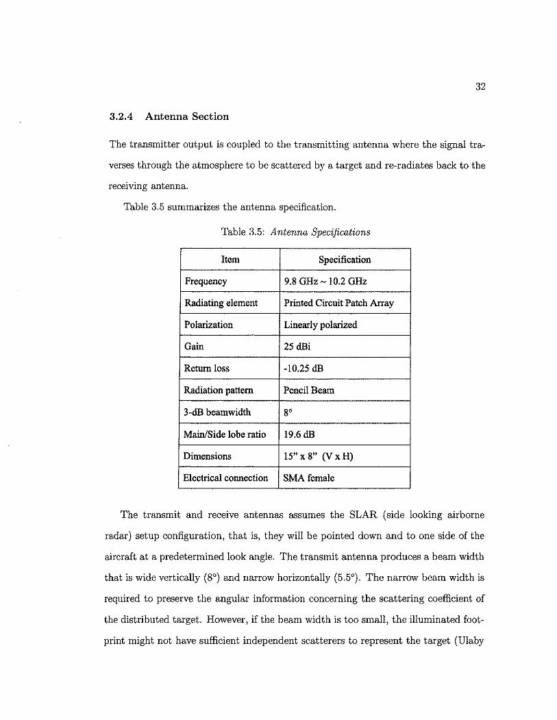
32
3.2.4 Antenna Section
The transmitter output is coupled to the transmitting antenna where the signal tra
verses through the atmosphere to be scattered by a target and re-radiates back to the
receiving antenna.
Table 3.5 summarizes the antenna specification.
Table 3.5: Antenna Specifications
Item Specification
Frequency 9.8 GHz -10.2 GHz
Radiating element Printed Circuit Patch Array
Polarization Linearly polarized
Gain 25 dBi
Return loss -10.25 dB
Radiation pattern Pencil Beam
3-dB beamwidth 8°
Main/Side lobe ratio 19.6 dB
Dimensions IS" x 8" (V x H)
Electrical connection SMA female
The transmit and receive antennas assumes the SLAR (side looking airborne
radar) setup configuration, that is, they will be pointed down and to one side of the
aircraft at a predetermined look angle. The transmit antenna produces a beam width
that is wide vertically (8°) and narrow horizontally (5.5°). The narrow beam width is
required to preserve the angular information concerning the scattering coefficient of
the distributed target. However, if the beam width is too small, the illuminated foot
print might not have sufficient independent scatterers to represent the target (Ulaby

33
et aI, 1982). On average, the power level figures (in Appendix A.2) show the first
side lobe level (SLL) from the main lobe is 19.6 dB and indicate that the return loss
is 10.25 dB at the center frequency.
The airborne antenna system must be lightweight and have a relatively small,
flat, streamlined physical profile to be considered practical. The microstrip patch
array best matches the required prerequisites of having the antennas mounted on the
outside of the fuselage of the aircraft. The receive and transmit antennas are identical
in every aspect and can be used interchangeably.
3.2.5 Data Acquisition Section
The data acquisition section consists of an AID computer card and the storage system
on the computer itself. The function of this section is to simply convert the IF
frequency analog signals into strings of digital data and store this information into a
memory device. Referring to the Nyquist sampling theorem, the sampling frequency
must be greater than twice the maximum IF frequency, iIFmax
is> 2frFmax (3.8)
The DIA card has a maximum sampling rate of 500 Msls, and since frF was
calculated from Equation (3.6) to be 30 MHz, this would imply the analog IF signal
could be properly recorded without aliasing. In Equation (3.6), all the parameters,
with the exception of the range (R), are fixed by the system. Since the range was
selected as 1 km as the maximum range allowed for this SAR, therefore the maximum
IF frequency cannot exceed 30 MHz. An ideal design would have the D I A and the
AID cards to have matched sampling rates, for everyone bit generated from the D I A,
the AID would be able to sample only one bit. If the AID sampling rate is greater
than the D I A generation rate, harmonics would appear during DSP and there would

34
be a risk of exceeding the on-board memory of the A/D card by gathering too much
information. Additionally, if too much data were gathered, there would be risk in
exceeding the maximum data transfer rate between the A/D card to the computer
storage disk, resulting in lost data. On the other hand, the penalty of having the
sampling rate of the A/D card being less than that of the D / A card would be a
loss of data. Since oversampling is inevitable with this system, the DSP can sample
average the data gathered with the A/D. This is accomplished by averaging 20 to
60 received pulsewidth returned signals. This averaging of the return signals reduces
system noise, but more over, it reduces the "environmental" noise. This is the noise
which is random and received from the surrounding terrain environment (Le. target
shifts, wind gusts, clutter movement, etc.).
Referring to Figure 3.1, it is necessary to have a lead-time of delay from when the
period starts to when the chirp pulse begins. The lead-time accounts for a minimum
time the veo needs to stabilize before constructing the LFM pulse, also for an
inherent delay between the D/ A and the A/D, and for the two-way travel time to the
target. It is also during this time period which the system transfers the data from
the on-board memory of the A/D card to the storage unit in the computer.
There is an on-board processor on each of the D/ A and the A/D cards, as such;
there is a mismatch in starting times (~ 100 nsec) from when the each card receives
the timing signal to when they start functioning. This mismatch is accounted for
during the trailing end where there is a dead period (after the chirp pulse) of the
waveform in Figure 3.1.

Chapter 4
Analysis and Results
4.1 Laboratory Test Results
35
Laboratory testing involves verifying, under controlled conditions that the RF and
digital hardware of the HRR is indeed functional within the parameters and specifi
cations outlined. Test procedures will verify the entire HRR radar design as a single
unit-under-test (UUT), as opposed to verifying each individual system component
as a stand-alone system. The UUT will consist of the four subsections as outlined
in Section 3.2: the waveform generation, RF, Receiver and Data Acquisition. The
antenna subsection will be bypassed during the laboratory-testing phase, but will be
tested and verified during field-testing. In the sections to follow, many of the same
procedures designed to test the compatibility of the individual component are used
to test and debug the inherent problems of system design. Therefore, rather than
testing and reporting duplicate results, the test procedures and plots to follow will
focus on identifying the shortcomings of the HRR radar system.
Testing identified two significant problems which appeared in the systems: (a)
identification of the low-frequency induced interference and implementation of a solu
tion to overcome this problem, and (b) identification of the signal IF gain-saturation
in the Receiver and Data Acquisition sections and provision of general guidelines to
obtain and process valid data.

36
In most of the test procedures, except where specifically noted, the output band
width of the veo will be limited to 40 MHz, rather than the full bandwidth of
400 MHz. The 10 % bandwidth restriction is a response to the AID sampling rate
limitation of 100 MHz. To avoid aliasing, the 40 MHz bandwidth is restricted to less
than the aliasing frequency of 50 MHz (fs ~ 2jm"",).
4.1.1 IF Gain-Saturation Problem
Once the RF components and digital circuitry are selected as the framework of the
system design, the system boundaries must be tested from which the complete system
will operate properly. One of the more significant problems of the HRR radar design
deals with maintaining a proper power level in the IF section of the design. The power
level of the received echo, at the receiver antenna, must be higher than the noise level
of the receiver in order to distinguish the target signal from the system noise. The
LNA will amplify the receive echo and the mixer downconverter will output the IF.
The power level of the IF range is adjusted by the AGe in the IF amplifier. The power
level of the signal available after the IF amplifier is the focus of this subsection. If the
power level is too high, then the input to the AID component will become saturated
and the acquired data will be incomplete and invalid. On the other hand, if the power
level is too low, the AID will sample noise and the data will be corrupted and invalid.
4.1.1.1 LFM Transmitted Signal and Power Spectrum (Saturation UUT)
Figure 4.1 represents the unit-under-test for this sequence of testing. This UUT
setup tests the functional compatibility of the transmit and receive channels of the
system design, as well as the data acquisition section. With the limited bandwidth
of 40 MHz, the combination D I A - veo generates the transmit chirp waveform of
approximately 9.8 GHz to 9.84 GHz.

Power -(9.8 GHz - 9.84 GHz) Divider
Load
Freq. Range: (10 MHz - SOO MHz)
Mixer / (JOMHz-40MHz) ? >
k---~~~~~~~ LNA
Figure 4.1: UUT- Testing LFM, Transmit, Receive and Data Acquisition.
37
With the coarse resolution of the two combined components allowing for a minor
variance in accuracy of starting/stopping at a specific frequency, the output range
might look something like 9.785 GHz to 9.832 GHz (as an example). The inputs to
the mixer are the LFM from the veo and a constant generated signal of 9.8 GHz
from the frequency synthesizer. The internal frequency bandpass range of the mixer
is 10 MHz to 500 MHz, so the output is a linear frequency signal of ~ 10 MHz to
40 MHz. An attenuation of 40 dB is provided at the output of the power divider so as
to limit the input power to the LNA. The attenuation simulates the signal strength
from a down-range target. The input voltage level of the A/D component is set at
200 m V, which is related to noise sensitivity of the acquired data.
In Figure 4.2, the top plot presents a time-domain signal as acquired by the A/D,
at a sampling rate of 100 MHz, and the bottom plot represents the Fast Fourier
Transform (FFT) of the signal representing the power spectrum density (PSD) of the
same signal.
It is clear from the time domain plot, the acquired data reveals a LFM wave
form. Point (!)represents the lowest frequency of the up-ramp, point @is the highest
frequency of the triangular waveform, and point ® is the lowest frequency of the
down-ramp.

Acquired Data
10~r-:-~ --~:~- ~-: " '-'---T-'-~- --r-' -----r·--------r--~----T----, ,
!' IHt \ 5 el;i'~~~'!-~-
1"1'" " I I
III ,il " , ' ·5 i~IWlf; i ..•. °lii' i
" , I I I I
.1Ol--";~_~--_ --_:, ____ .. _._: __ . ____ ~._.~ o 200 400 600 800 1000 1200
Power Spectrum Density
, , , ,
, , , '400·";c.;--7:,000= --1-~--2000
: ~ .... t .... ·,i·,';,:,! ii1Ji(f.i;iRl1iil;i~ \If'Mr~M''"1(;~J]\Fr .... ~ ... . 40 f· ..: .... ;: 11'/,1'1111~~ilfl n i .. !: " + "~!lrillt';l"i'h" ...... ~ ... ,.
'Il 30~'~i~flM:~~r:~fi' ~ ~:iL~I .. : r: f· "1':' .I~:~ I!:u~f·'~·Hj~~:\~~lt~¥~\~1 2Oh,t111.~"1In, ... __ .L. --." •• --". -- ._L _. - -"- -- - --I~'SM"rl'.h't ,o n~~~i,:?·_:~,';1;:.'J~ _i., ___ .~. ____ .: -.- .:,_ -.- -.- __ :". ____ ol,' _ ' !Ti';"i~:,'~ti(l J~_ r ----"-'-!--
, , ,
frequency (MHz)
Figure 4.2: VCO-50dB·LNA·9.8GHz·Mixer·200m V.
38
It would be ideal for the lowest frequency, points (Dand ® to reside at the begin·
ning of sampling and at the end of sampling the data, respectively. However, due to
inability of the chirp generation section to generate an exact 9,8 GHz to 9.84 GHz,
the mixer will output the difference between the static 9.8 GHz and the LFM from
the veo.
The PSD plot shows the bandpass frequencies starting at baseband and cutting
off around 32 MHz. This plot should ideally display a bandpass frequency range of
~ 10 MHz to 40 MHz. There are two reasons for this disparity, the first is explained
by chirp generation section limitations of providing exact start/stop frequencies, and
the second is due to the internal passband of the mixer. The passband specification
of the mixer indicates a range of 10 MHz to 500 MHz, however, the 3·dB cutoff of
this BPF could allow for slightly more, or less, signal to pass through the passband.

39
The following plots in Figure 4.3 are included to illustrate the importance of the
attenuation level (i.e. simulative of target strength) of the transmitted signal and the
input voltage level of the A/D. Using the same UUT setup, increase the attenuator
to 60 dB and lower the input voltage level to the AID component.
Acquired Data
600 800 1000 1200 1400 1600 1800 2000
Figure 4.3: VCO-70dB-LNA-9.8GHz-Mixer-50m V.
In Figure 4.3, the time domain plot exhibits a lower overall voltage level in the
acquired data, as well as the waveform appearing to be coarser than previous. This
fact is explained by the LN A receiving weaker signal strength (through added attenu
ation). The PSD plot exhibits a lower SNR level compared to the previous plot. With
the input voltage level decrease on the A/D, the threshold level of the input signal
is limited while the noise level is allowed to rise. This effect reduces the dynamic
range of the input signal in reference to the noise floor, thereby lowering the SNR.
Although not as clear as in the previous PSD plot, a passband is still visible with a
similar cutoff frequency.

40
The conclusion interpreted from both sets of plots provides verification for the
functionality and interface of each component in the UUT. In addition, it points out
the effects of the attenuation level to the LNA and the input voltage level to the AID
component.
4.1.1.2 Saturation UUT - Include The IF BPF
Figure 4.4 represents the unit-under-test for this sequence of testing. This UUT
setup includes the intermediate frequency bandpass filter. The UUT will test the IF
passband boundaries of the system design.
26 MHz ± 3,5 MHz
Power 9.8 GHz - 9,84 GHz) Divider
Load Freq. Range:
(10 MHz- 500 MHz)
Mixer /
LNAI<---'
Figure 4.4: UUT- Testing IF passband.
The UUT setup is identical to Figure 4.1, with the addition of the IF BPF, having
a center frequency of 26 MHz and a bandwidth of 7 MHz. The input to the BPF is
10 MHz to 50 MHz from the downconverter mixer, and the output frequency range
of the BPF is 22.5 MHz to 29.5 MHz. Figure 4.5 shows plots of the AID acquired
data in the time domain, and the FFT of the sampled data representing its power
spectrum.
The frequency range of the generated chirp waveform is ~ 9.8 GHz to 9.84 GHz
and the static synthesized frequency is at 9.79 GHz. Shifting the synthesized fre
quency to 9.79 GHz allows the passband of the downconverter to start at 10 MHz,
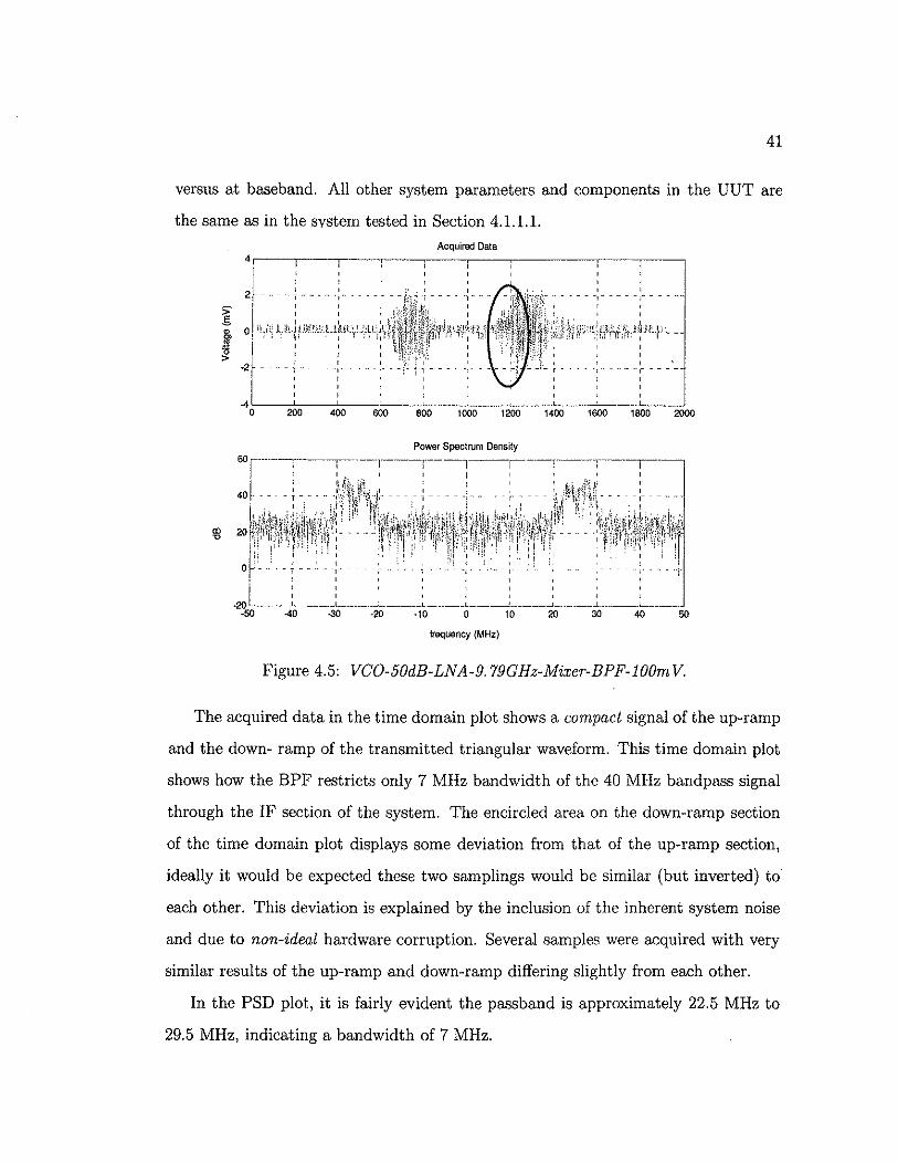
41
versus at baseband. All other system parameters and components in the UUT are
the same as in the svstem tested in Section 4.1.1.1. Acquired Data
4r---~---'----~--__ ----r---__ ---.----~---r---,
2~-i---: , ,
J °1))!il':'.I:.;!\;iUfr~~v . . 2----:----:- , ,-, 4~1 ~~ ____ ~~~ ___ ~ ____ ~~~
o 200 400 600 800 1000 1200 1400 1600 1800 2000
Power Spectrum Density
frequency (MHz)
Figure 4.5: VGO-50dB-LNA-9. 79GHz-Mixer-BPF-I00m V.
The acquired data in the time domain plot shows a compact signal of the up-ramp
and the down- ramp of the transmitted triangular waveform. This time domain plot
shows how the BPF restricts only 7 MHz bandwidth of the 40 MHz bandpass signal
through the IF section of the system. The encircled area on the down-ramp section
of the time domain plot displays some deviation from that of the up-ramp section,
ideally it would be expected these two samplings would be similar (but inverted) to
each other. This deviation is explained by the inclusion of the inherent system noise
and due to non-ideal hardware corruption. Several samples were acquired with very
similar results of the up-ramp and down-ramp differing slightly from each other.
In the PSD plot, it is fairly evident the passband is approximately 22.5 MHz to
29.5 MHz, indicating a bandwidth of 7 MHz.

42
The conclusions interpreted form this set of plots provides a high confidence level
for the integration of the IF BPF into the system design.
4.1.1.3 Saturation UUT - Include The IF Amplifier
Figure 4.6 represents the unit-under-test for this sequence of testing. This UUT setup
includes the intermediate frequency amplifier with automatic gain control (AGC). The
UUT will test the effects of gain-saturation levels from the IF amplifier to the system
design.
G---< IF Amp
20 MHz - 60 MHz
-(9.8 OHz-9.84 OHz)
Mixer
LNAI<---'
Figure 4.6: UUT-Testing IF Amplifier and AGe Saturation Level.
The UUT setup is identical to Figure 4.1, with the addition of the IF amplifier
having a center frequency of 30 MHz and a bandwidth of 10 MHz. Controlling the
saturation level of the IF amplifier output is essential to maintain a proper voltage
level to the input of the AID component to adequately sample the data. The AGC
of the IF amplifier has a dynamic range of 70 dB. The amplifier will exhibit no gain
when there is a -4 V at the input AGC port, in turn, the amplifier will boost the
received signal the full 70 dB when the AGC port is either grounded or there is no
input. The amplifier will not differentiate between a valid signal and noise, rather it
will amplify whatever the signal is present at its input port. The input frequency to
the amplifier is 20 MHz to 60 MHz from the mixer downconverter, and the output

43
is 25 MHz to 35 MHz due to the internal passband of the IF amplifier. All other
system parameters and components in the UUT are the same as in the system tested
in Section 4.1.1.1.
Acquired Data
200 400 600 800 1000 1200 1400 1600 1800 2000
frequency (MHz)
Figure 4.7: VCG-50 dB-LNA-9. 78GHz-Mixer-IF-l0v (Gain 70 dB).
Since a ground to the AGe port boosted the input from the IF amplifier 70 dB,
the input voltage level of the AID component was raised to the maximum 10 volts.
This test demonstrates the need to keep the AGe gain adjusted to proper levels
relative to the signal strength of the received signal from the target. If the receiver
antenna receives a strong signal from a high reflectivity target or a close-in targ<')t,
the incoming signal will be strong and the need to reduce the AGe gain to avoid
saturating the input to the AID component is essential. The time domain plot in
Figure 4.7 shows a signal that is clipped at the top and bottom, resulting from the
applied 70-dB AGe gain and thereby saturating the AID input. As a result of this

44
saturation, the power spectrum in the PSD plot is unable to clearly show the proper
passband SNR.
After lowering the AGe gain below the maximum level, the time domain plot in
Figure 4.8 displays the sampled signal that is not saturated and the PSD plot of a
power spectrum with a clear passband.
" .' ~ __ :,\ - .• ..1" , , , , 10 - - __ 1 _ .!. , , , ,
Acquired Data
Power Spectrum Density
, , , - - .• _I. ..1_ , , ,
... - - _I.
10
frequency (MHz)
, , ---I-----C---
, , , ,
1600 1800 2000
--,-----'-._--I I I I:i , , ,
. . l ___ , _. .. _ 1_ , , , , ,
30 40 50
Figure 4.8: VCO-50dB-LNA-9. 78GHz-Mixer-IF-AGC2v-l0v(Gain < 70dB).
The PSD plot exhibits a passband of approximately 20 MHz to 45 MHz, which is
slightly higher than the internal passband of the IF amplifier (25 MHz 35 MHz). As
previously stated, this irregularity can be explained by the 3-dB cutoff of the internal
BPF of the IF amplifier.
4.1.1.4 Saturation DDT - Include The LNA And IF Amplifier
Figure 4.9 represents the unit-under-test for this sequence of testing. This UUT setup
represents the complete system design. The UUT will test the compatibility of all
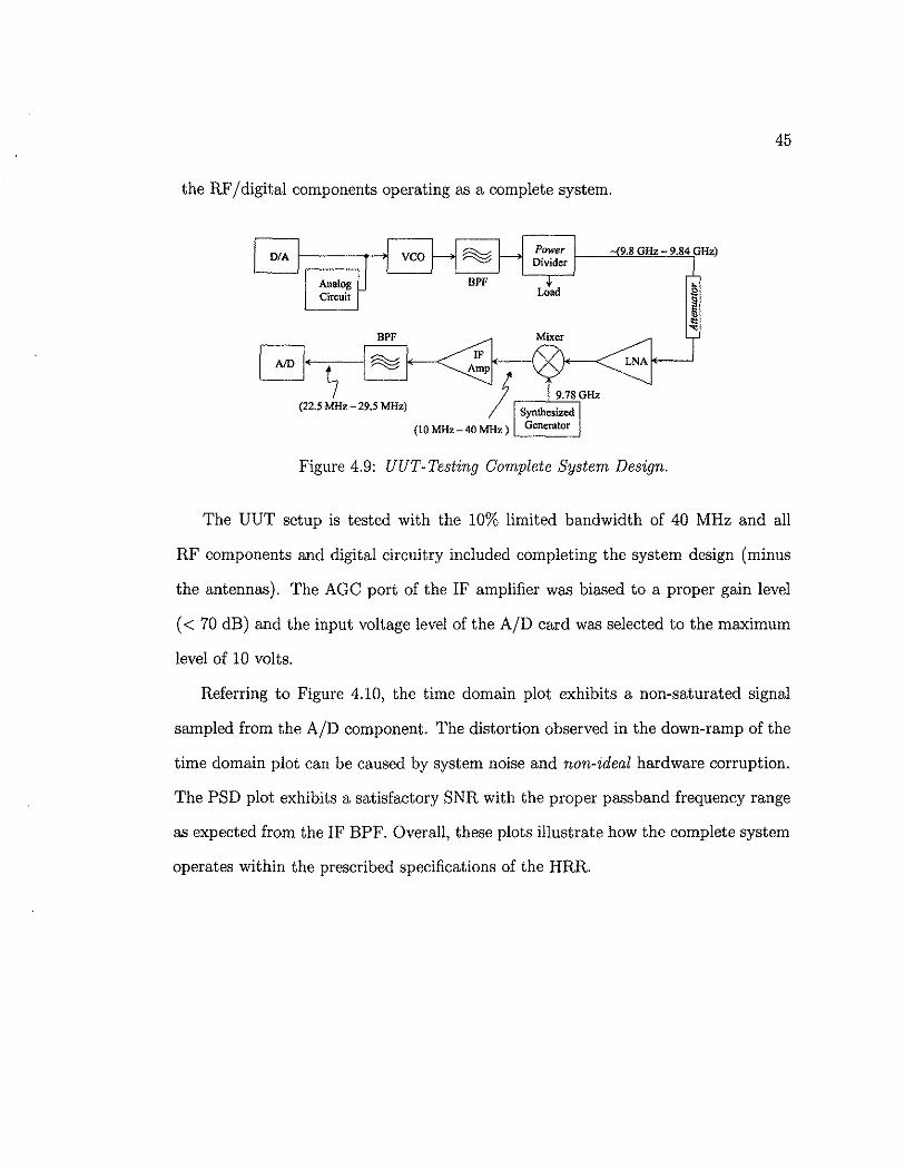
45
the RF I digital components operating as a complete system.
9.8 GHz - 9.84 GHz)
LNAI<----'
Figure 4.9: UUT- Testing Complete System Design.
The UUT setup is tested with the 10% limited bandwidth of 40 MHz and all
RF components and digital circuitry included completing the system design (minus
the antennas). The AGe port of the IF amplifier was biased to a proper gain level
« 70 dB) and the input voltage level of the AID card was selected to the maximum
level of 10 volts.
Referring to Figure 4.10, the time domain plot exhibits a non-saturated signal
sampled from the AID component. The distortion observed in the down-ramp of the
time domain plot can be caused by system noise and non-ideal hardware corruption.
The PSD plot exhibits a satisfactory SNR with the proper passband frequency range
as expected from the IF BPF. Overall, these plots illustrate how the complete system
operates within the prescribed specifications of the HRR.

46
Acquired Data 05
1
I o ~"J teLl Wll.::~{'il.11 .. c>",,' ,,,;0' it :! -, : f
·0.5~-....,-'-.,----,.L---'----'---' __ ---'-__ -,L_----c:L-_-,-'L.._-l o 200 400 600 800 1000 1200 1400 1600 1800 2000
Power Spectrum Density
4.1.2 LOW-FREQUENCY Interference Problem
In HRR radar systems, operating in the microwave region, it is common to find
residuals of undesired low frequencies. These residuals become problematic since
they induce harmonics within the system, and they also extend the minimum range
of the close-in target where the system can begin to acquire valid data. These low
frequencies usually reside in the kilohertz range, which can be on the same scale of
magnitude of the IF range, and thereby inducing itself (or its harmonics) along with
valid data.
In Section 3.2.3, the relationship between the IF frequency and range was ex
plained with Equation (3.6). It is repeated here for convenience.

2ER iIF=-cT
47
( 4.1)
The system variables E, c and T are grouped as a single constant a, leaving the
following equation. iIF=aR ( 4.2)
From Equation (4.2), it is easy to see that iIF is directly proportional to range.
When the IF frequency is corrupted with low-frequency effects, there is a proportional
range (distance) which the system will be unable to use as valid data, thereby placing
a higher limit on a minimum range the system can begin to detect a target.
4.1.2.1 Identifying Low Frequency (Low Frequency UUT)
Figure 4.11 represents the unit-under-test for this sequence of testing. This UUT
setup test will identify the low frequency and locate the origin of where it is being
induced into the system. The UUT consists of the minimum required RF components
to generate a 40-MHz bandwidth chirp-waveform and simultaneously acquire the IF
through sampling with the AID component.
Analog Circuit
System Bandwidth
-OHz
Power Divider
Figure 4.11: UUT- Testing the Low Frequency System Component.
The power divider provides the same generated chirp signal to both inputs of
the mixer downconverter; therefore the mixer IF is expected to output at baseband.

48 Acquired Data
o r~'-N-"-"r'---'-'!""-'-'~"~"-~'-'--"--:---'''-'-'-!--"~--'--"-"~~-'-T"'-'.--:-'-'-'-';----
.o.o2f:f~Tf"' 7"" - .... - -:- - - .... -~ -- - .... ~ - - - .... ~- ........ - -~ .... _ ........ .L _ .... _ .... _1 __ ........ -:,LllflT--004 ~}, dlflr~j -:- --- , -, - -: il!1!~d'"'' --O,oor- --:"~-'--jiij{(:,- -! -: -, ::i:fl~jl;,j---~·:·······~
-O.08~ - ........ -: .... _ ........ -:- ~ ~ ~ rr,1)rr1w:!- ............ :- ........ -ll~ltN~i~~,ll:- -' ............ -............ -: ........ --0
0.11----:- ":- ~··:·'-·-~-.1'··(;·;:H~-:'-'··'~···~ '._--, -:-..Q.12 L._ ..... ___ ..L~ ____ ._._L ...... ___ .1. __ ._,,~.J~ _ .... ~ ... ~L~ __ : ........... J. ....... "_, ___ ._L. _____ --' __ . ___ L_~
o 200 400 600 BOO 1000 1200 1400 1600 1800 2000
Power Spoctrum Density OOr---,---.-------,----r--~----,_--T,---,---.
I , I I t I I I I I I I' I I I I
:~:: _: i ::-: r-::~:::::: -:: r:::r -:::::: -: r:: :~:::: 2Q r'tiiifllf,;~IS!!'I· .. iliJil'*;~N~W,'il,i;tlilhNt)li\";'i;f:'~~!fJ! i;M~i~4~~Wir('if!\1,'\\VWI\I;'r~i\bifW~lfW\~j o " _ ~.~:;~~ 1.!~ 'It ___ ,_,[,_ ! ,_!_! ['~l_r_j! :! ~ : p!~i:: f;!~ .~ :_':( :!_:~'!! ~i_'
-20 1 I I , I I I I I I
~ ~ • • ~o 0 10 2Q m ~ ~
frequency (MHz)
Figure 4.12: VCO-BW40-PD-Mixer-2V.
Power Spectrum Density
frequency (MHz)
Figure 4.13: VCO-BW40-PD-Mixer-20m V.

49
The two interconnecting cables between the power divider to the mixer are of the
same type, have the same connectors and are virtually the same length. Having
identical cables reduces the possibility of inducing phase mismatch (via reflections)
at the component ports and indirectly producing system noise. Two set of plots are
listed in Figures 4.12 and 4.13, the differentiating factor between each set is the input
voltage level for A/D sampling.
The time domain plots in Figures 4.12 and 4.13 indicate the presence of a sta
ble low frequency signal. The frequency of this signal is 1/((216+215)*400 ns) ""
6 kHz. There are two significant factors contributing to the low frequency; the dis
crete step intervals from the D / A to the VCO generating the transmit waveform,
and the impedance mismatches (Le. reflections) at the interface between RF system
components (Le. the RF interface).
More specifically, the low frequency interference originates at the VCO due to the
discrete step output frequency versus a linear ramp frequency output and including
the cross coupling between the two ports of a non-ideal power divider. It is not
the RF alone that generates the low frequency, rather the RF interface, which adds
constructively or destructively to the system. A basis for this conclusion resides in
the fact that noise is random and virtually impossible to replicate, whereas the RF
interface will produce similar results each time. This reasoning supports why similar
(but not exact) power spectra near baseband are observed in each of the PSD plots.
The PSD plots from Figures 4.12 and 4.13, indicate no higher frequency components,
except close to DC. The power density observed near baseband, is a product of the
time delay invoked by mismatched cables between the power divider and the mixer.
Several measurements were taken with differing mismatched cable lengths and each
displayed a shifted power spectra near baseband.

50
The plots in Figure 4.14 involve widening the transmission bandwidth to its
full range. By expanding the testing procedure to include the entire bandwidth of
400 MHz, the test will demonstrate similar outcomes as with the 10% bandwidth.
More importantly, this broader testing profile will verify that the system's hardware
and software do function correctly under normal operating system conditions.
,j ~; :'1 i I " 0
·50 "'0 -30 ·20 ·10 0 10 20 30 40 50
frequency (MHz)
Figure 4.14: VCO-BW40-PD-Mixer-20m V.
The time domain plot continues to exhibit a low frequency component under the
full system bandwidth. The frequency is different than the previous test which can
be attributed to the coarse resolution of the D I A discrete step resolution and aliasing
at the AID component.
4.1.2.2 Low Frequency UUT Changing the AID Sampling Rate
Figure 4.15 represents the unit-under-test for this sequence of testing. This is the
same UUT configuration that was used in the previous Subsection 4.1.2.1 and will

51
Power Spectrum Density
I I 'I I • I
, "
frequency (MHz)
Figure 4.15: VGO-BW40-PD-Mixer-500m V-Sampling Rate 500 MHz.
test what effect the AID component will have on the low frequency interference within
the system. The difference in this configuration from the previous configuration is
the increase of the sampling rate of the AID component from 100 MHz to 400 MHz.
Figure 4.15 displays the time domain plot exhibiting no discernable difference
from the time domain plot in Figure 4.13, which is sampling at the system default
rate of 100 MHz.
Therefore, the conclusion to exclude the AID component as a contributor to the
induced low frequency is valid.
4.1.2.3 Low Frequency DDT - Including the IF BPF
Figure 4.16 represents the unit-under-test for this sequence of testing. This UUT
setup test will include the IF bandpass filter to confirm that the low-frequency effect
will be filtered out before the AID begins sampling data. The UUT will be tested

52
with the chirp bandwidth of 40 MHz (9.8 GHz - 9.84 GHz) and then will be repeated
with the full bandwidth of 400 MHz (9.8 GHz - 10.2 GHz).
In the previous Subsection 4.1.2.1, a low frequency component was identified to
be present in the system as early as in the signal generation section of the design.
Power Divider
-{9.8 GHz - 9.84 GHz)
Figure 4.16: UUT- Filtering Out the Low-Frequency Effect.
This UUT has included the IF BPF to filter out this low frequency, as well as those
frequency components due from the power divider/mixer cable mismatch. The plots
of Figure 4.17 and Figure 4.18 represent the sampled data with a system bandwidth
of 40 MHz and 400 MHz, respectively. In both of the time domain plots in Figure 4.17
and 4.18, there is no valid signal. The signals observed in both cases are very small
and are attributed to system noise. The PSD plots both exhibit various spikes in the
power spectrum, but they are random and possess no significant value. Therefore,
the conclusion taken from this test confirms the IF bandpass filter can satisfactorily
eliminate the low frequency components.

:;g
I
Power Spectrum Density
frequency (MHz)
Figure 4.17: VCO-BW40-PD-Mixer-BPF-50m V.
Acquired Data
Power Spectrum Density
j "I '.," , ,
·20 I _____ ._._.~---.. ---~--.~~~~-.- __ ._~_ ·50 -40 ·30 ·20 ·10 10 30 40
frequency (MHz)
Figure 4.18: VCO-BW400-PD-Mixer-BPF-50m V.
53
50

54
4.1.2.4 Low Frequency UUT - Including the RF Amplifier
Figure 4.19 represents the unit-under-test for this sequence of testing. This UUT
setup test will include the RF amplifier to confirm the effects of this system component
will not be additive to the low frequency problem. The RF amplifier will boost
the transmitted signal to +40 dBm, and connected to the output will be a 40 dB
attenuator to lower the amplified signal, thereby avoiding damage to the mixer.
Power RF Divider Amp
G+-----------{ Mixer
Figure 4.19: UUT Testing the Effect of the RF Amplifier.
This configuration tests what effect the addition of the RF amplifier will have on
the system. The UUT is tested with the system bandwidth limited to 40 MHz.
Even with the addition of the RF amplifier and attenuator, the time domain plot
in Figure 4.20 displays how the low-frequency effect is still present and is quite similar
to the UUT without the amplifier. The PSD plot exhibits no valid power spectra,
except close to baseband, which has previously been explained as the cable mismatch
between the power divider and the mixer. Therefore, it is safe to conclude the RF
amplifier contributes nothing to the low-frequency component.
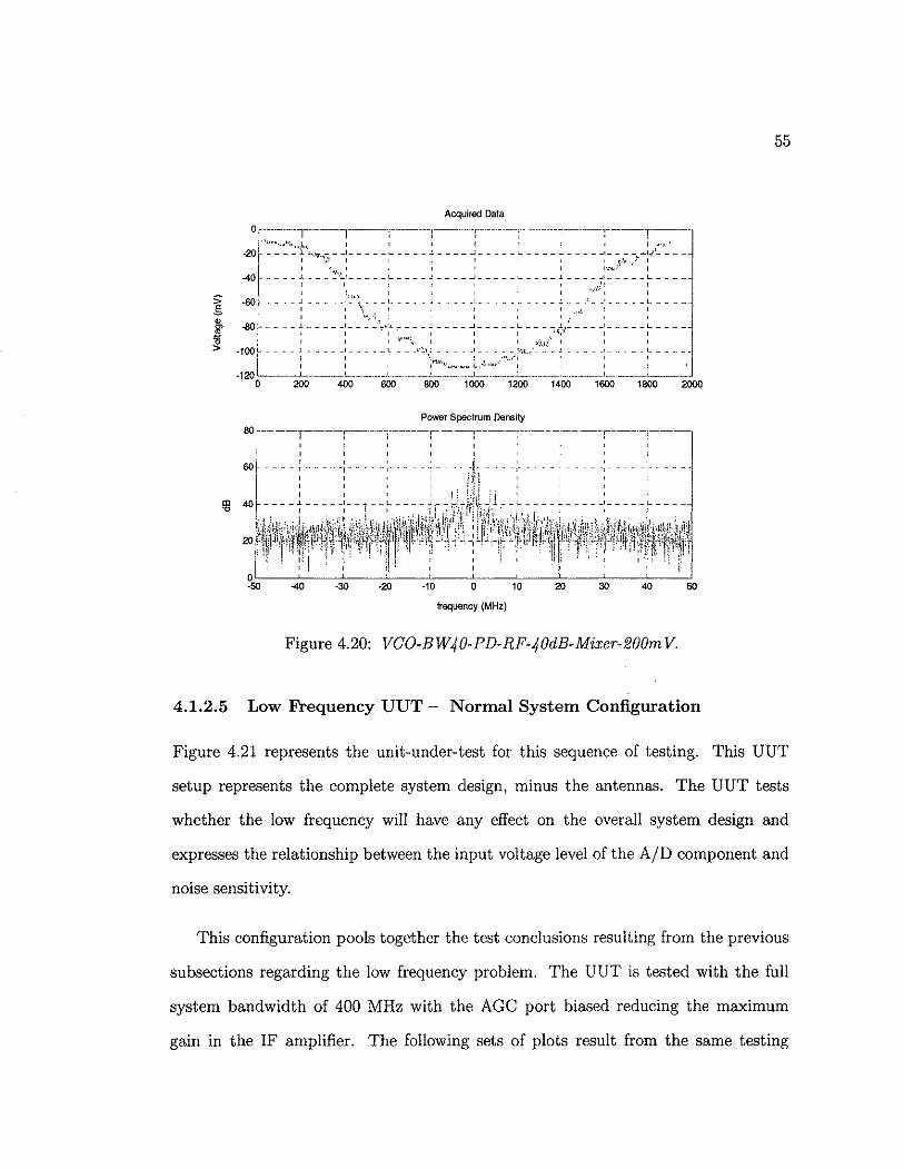
55
Acquired Data
s rl,·J.·T.·.:····r'·······.~I;·t-g l I I , , I , J ."c' I
<II -00 ____ ~ _____ : ____ •• :~'" ___ ~ _ ___ ~ ____ _ ~ ___ ""~,!. ____ : _____ ~ ___ _
>
E I I , ' I I I ,\,~ I I
<.J i I I 1 'I"';' I I I 1 I I
~::l~l~~~L~~.~.,~.:·_.~_~~:~::~;_;:~:~_._~~_~. ___ ~~ .. ~ __ : __ :~~!~_.~~~: o 200 400 600 800 1000 1200 1400 1600 1800 2000
Power Spectrum Density
, , , , ----T- '-,--" '0j""
-10 o 10
frequency (MHz)
Figure 4.20: VGO-BW40-PD-RF-40dB-Mixer-200m V.
4.1.2.5 Low Frequency UUT - Normal System Configuration
Figure 4.21 represents the unit-under-test for this sequence of testing. This UUT
setup represents the complete system design, minus the antennas. The UUT tests
whether the low frequency will have any effect on the overall system design and
expresses the relationship between the input voltage level of the AID component and
noise sensitivity.
This configuration pools together the test conclusions resulting from the previous
subsections regarding the low frequency problem. The UUT is tested with the full
system bandwidth of 400 MHz with the AGe port biased reducing the maximum
gain in the IF amplifier. The following sets of plots result from the same testing

IF Amp
Power Divider
Mixer
J LNA~--'
Figure 4.21: Testing Normal System Configuration.
56
procedure; however, the one variable factor is the input voltage level to the AID
component. The time domain plots in the Figures 4.22 through 4.25 show the AID
sampling virtually zero input signal. This concludes the system as a whole does filter
out any residuals of the low frequency. On the other hand, the PSD plots illustrate
the effects of selecting a proper input voltage level to the sampling AID component.
I' -, - - - 1- -, , , ,
Acquired Dala
Power Spectrum Density
"r-
-20-',-----'~-----.3!O~ --..... -.~ ----70--
frequency (MHz)
Figure 4.22: VCO-BW400-PD-50dB-LNA-MIXER-IF(AGC3v)-BPF-2v.

57 Acquired Data
O.02r~----r-·--1----r-·---: ----r----r--O.015 r-- --: .. _;- --;- --" -~ .... ---: -----;--- --.~.---
r i--I-, -L____ ••• L __
Q01 ____ ~ __ ~-~- ____ ~----~----~-----h--- ~-----,-----~----
Power Spectrum Density
frequency (MHz)
Figure 4.23: VCO-BW400-PD-50dB-LNA-MIXER-IF(AGC3v)-BPF-lv.
Acquired Data
Power Spectrum Density
, , •• - T •..•.• -I • r - - - - "1"
, , -I· . - - ,- -
-30 ·20 ·10 o 10 50
frequency (MHz)
Figure 4.24: VCO-BW400-PD-50dB-LNA-MIXER-IF(AGC3v)-BPF-500mv.

58
Acquired Data 6
, , , , - -I _. .. 1-
'> .s ~ '5 > , , , ,
- -I - - - - ,- - - - -', - - - - -,. --, , , , -4
0 0.2 0.4 0.6 0.8 1.2 1.4 1.6 1.8
Power Spectrum Density
frequency (MHz)
Figure 4.25: VCO-BW400-PD-50dB-LNA-MIXER-IF(AGC3v)-BPF-200mv.
It is evident in Figures 4.22 - 4.25, the PSD plots display different power spectra
as the input voltage levels decrease from 2 volts to 200 millivolts. At higher input
levels, the AID samples a wider dynamic range of power spectra above the noise
floor. This is evident in Figure 4.22, with the input level at 2 volts, the PSD shows
random spikes in the power spectrum that originate from the discrete output steps
at the yeo. In Figure 4.24, as the selected input level lowers to 500 millivolts, a
much narrower dynamic range is sampled by the AID and evidence of noise begins to
appear in the PSD plot. When the input voltage level is lowered to 200 millivolts, the
power level of the signal is on the same order of magnitude as the noise floor and the
PSD plot in Figure 4.25 displays band-limited amplified noise. At these lower voltage
levels, the AID component becomes quite sensitive to detecting the low level signals
and care must be taken not to mistake the power spectrum of band-limited noise as

59
a valid low-level signal. Of the four sets of plots, Figure 4.23 shows the best selection
of input voltage level to be at 1 V for the conditions given in this DDT. Here, the
time domain plot exhibits a virtual zero input signal and the PSD shows no power
spectrum.
4.1.3 Laboratory Testing Conclusions
In the previous subsections, the HRR radar system design was tested to identify and
understand the inherent problems associated when RF components, digital hardware
and controlling system software interface one another at X-band frequencies. Testing
to understand the relationship between target reflectivity, return echo strength and
signal saturation is essential to aid interpreting acquired data and avoid acquiring
erroneous data. The AGC control governs the level of gain the IF amplifier would
boost the incoming signal. Too much gain from the IF amplifier would saturate a
valid input signal to the AID component, whereas too little gain would not con
tribute to a proper level of signal-to-noise ratio. The level of gain is dependent on the
power level of the signal return and should be adjusted according to the environment
or conditions the measurements are taken. Similarly, identifying the low frequency
component in this system design is essential to understanding the boundaries or lim
itations the HRR radar can operate within. There were several factors identified
contributing to the most significant amount of noise to the system; the D I A-VCO
discrete step interval waveform generation, the RF interface between RF components
resulting in reflections, and cable mismatches adding time delays in certain signal
paths. The low frequency places a limitation on close-range measurements (ffF <X R
), i.e. the minimum distance the radar can illuminate a target and acquire valid
data. The inherent low frequency was filtered out via the IF bandpass filter. Lastly,
the AID component was tested and a relationship was identified between input volt
age levels and the sensitivity to low-level signals. Higher input voltage levels are
60
necessary when there exist higher power levels of the signal being sampled. As the
input voltage levels become higher, also comes a wider dynamic range in the power
spectrum to be sampled. When the input voltage level decreases, the narrower the
dynamic range becomes and the A/D becomes more sensitive to noise. Similar to the
conditions for AGe in the IF amplifier, the input voltage level to the A/D component
should be properly adjusted to the system configuration and environment in which
the measurements are made.
4.2 HRR Radar Data Processing
The data acquired by the A/D converter is related to the reflectivity of the target as
received by the radar receiver. This data are stored as a raw digital format that cannot
provide intelligible information in its current form. Therefore, some manipulation to
this data format is required to interpret what the radar is seeing downrange. The
data reformatting takes place in software data processing. There are two software
applications that are used to acquire and process the HRR radar data; these are the
LabView software interface program and Matlab, a mathematical software program.
Lab View is the graphical user interface used to adjust system parameters, on-the-fiy,
while acquiring and storing the data onto a storage media. Matlab will use the stored
data to provide digital filtering, pulse averaging, Fast Fourier Transforms and produce
both time domain, and PSD plots.
4.2.1 Data Structure
The generation of transmitted waveform is described from a hardware viewpoint in
Section 3.2.1. However, the data structure of the transmit and receive waveforms is a
more detailed description of generating data and acquiring data from a point/sample
viewpoint.

61
4.2.1.1 Generating Pulse
The data structure of the transmitted and received waveforms can be explained by
referring to Figure 3.1 from the previous chapter. There is an elapsed time from
the beginning of the transmission to the beginning of the LFM chirp of 2 ms. This
elapsed time is necessary to account for the stabilization time of the yeO, the intrinsic
time delay between the AID and the D I A components and the two-way round trip
time delay of the transmitted signal. The number of points for this elapsed time is
2 ms * 5 MHz = 10,000 points from the DI A. Figure 4.26 shows the parameters for
the generation of the LFM chirp.
Tf1Irum.t
210 steps '*400 M 215i1e-p;"'400M
Receive
ru",:lli i SavedDiIta , .
Figure 4.26: Parameters of the LFM Chirp waveform.
The received waveform is a virtual replica of the transmitted waveform, with a
time delay of f>.t = td = 2RI c, equating to the two-way round trip time the transmit
ted wave takes to propagate to the target and return to the radar receiver. The D I A
converter generates samples at a rate of 5 MHz (200 ns). The RF veo does not use
the full resolution of its output range, rather only those points between 584 and 800,

62
equating to 10.2 GHz and 9.8 GHz, respectively. This difference is 800 - 584 = 216
steps from the D / A, and since there is an up-ramp and a down-ramp to the transmit
ted wave, the initial number of steps to create the up-/ down-ramps are 216 + 215 =
431 steps. However, since each step consists of two generated sample points, the total
number of generated sample points for the waveform is 431 steps * 2 pts/step = 862
points. As a result of the internal time delay of the D / A, this component cannot be
relied upon to terminate the waveform transmission at a consistent end point every
time. This is the reasoning for the arbitrary dead time sometime after the end of the
down-ramp and the start of the following period. Summarizing the data structure of
a complete period of the transmitting waveform is given in Figure 4.27.
F(t)
2.0ms (10.000 pts)
PRI= 2.5 ms (12.000 pts)
dead space
~\ 86.4 i" 86.0 i"; 226 i" i
(432pts) (430pts) (1130pts)
Figure 4.27: Point Data Structure of the Transmitted Waveform.
4.2.1.2 Acquiring Data
The A/D converter is responsible for acquiring the return data from the receiver in the
form of sampling this data. The sampling rate of the A/D is set for 100 MHz. Once
the D / A starts generating the waveform for transmission, the A/D begins to acquire
the data from the IF bandpass filter. Figure 4.28 shows the number of sampling
points in each section of the waveform. There are a total number of 243,840 points
being sampled by the A/D, however only a fraction of this is actually being saved.

63
The LFM chirp return appears after a time delay equal to the two-way propagation
of the transmit signal, and it is at this time when the AID begins to save the data
into storage. Referring to Figure 4.26, the length of time the AID actually saves
the sampled data is equal to the time pulse duration of the chirp wave minus the
time delay of two-way propagation from the transmitted signal. In other words,
t:>.t = 2Rlc = (2 * 20m)/3E8 = 133.3 ns or equivalently, 133.3 ns * 100 MHz =
13 sample points. Therefore, the total number of saved sample points per transmitted
period is 17,240 - 13 =17,227 points.
2.0ms'" 100 MHz '" 172.4)lS • 100 MHz '" 200,000 pts 17,240 pts
266)lS ... 100 MHz "" I 26.600 pts
Figure 4.28: Sampled Data Points from received waveform.
In summary, the total number of sampled points from the AID components is
243,840 points, but only 17,227 points of this total are actually being stored for data
processing. It is during this period of saved data which the frequency difference
between the transmitting and receive signals can range profile be extracted.
After the data are acquired and stored onto a storage disk, Matlab will process
this data through a software program that will develop the various plots representing
the data. The data processing involves averaging a certain number of return wave
form periods to filter out some of the signal randomness (caused by random noise,
changing environmental conditions, etc.) With the amount of over-sampling the AID
component samples, the number of times the return periods are averaged varies from
data to data to develop the most representative example of the data. In addition

64
to the filtering out some of the random noise components, the processing software
program also throws away a portion of the beginning acquired data. The reasoning
behind a portion of the return signal being discarded is cut out that data that might
be corrupted by the veo not having enough time to settle down. Again, like the
number of return period averaging, the amount of sample points discarded is selected
on a case-by-case basis to best represent the target data.
4.3 Field Test Results
Field-testing of the HRR radar system involves taking the theoretical design out of
the laboratory-controlled environment and subjecting the radar to practical environ
mental stimuli. It is during field-testing when the researcher learns of the shortfalls
and inaccuracies of the radar design, which comes about from missed parameter as
sertions to over-optimistic assumptions. It is also at this stage when the limitations
of the radar system are revealed and additional adjustments in hardware, or in ex
pectations, are warranted. In the following subsections, the HRR radar will resolve
a single trihedral, to serve as a reference target, and then include a secondary tri
hedral that will vary in range in relation to the reference target. Another test will
replace the secondary trihedral with a different type of a target, namely a pickup
truck. These testing configurations will provide information on range resolution that
the HRR radar will be able to resolve.
4.3.1 HRR Radar Profiling Results
Figure 4.29 illustrates the target arrangement profile used to measure the range res
olution of the HRR radar system.
The HRR radar hardware is mounted on a boom and is elevated 20 meters above
the ground. In every field test configuration, there is a reference trihedral target

65
Down Range Secondary , . Target r" ............. C\:,~:;:::~:: ... T
Rx \. Target :
r··················~;:~o..j / 20m ., : :,
\ !
.. ~-..,/
\
Radar Cross Range
Figure 4.29: Target arrangement profile.
located 20 meters from the base of the boom carrying the radar. The combination of
the elevation distance, along with the distance to the reference target, will provide a
grazing angle of 45° , once the tilt of the radar is adjusted for maximum signal power
return. Due to the height limitation of the HRR platform to such a shallow elevation,
there is a corresponding limitation to the distance the targets can be set down range.
If the targets are set too far down range, then the grazing angle will become too small
and difficulty in resolving these targets becomes an issue. For example, the interfer-
ence of two-way bounce from the terrain surface increases, increased clutter from the
terrain becomes additive with the return signal or even the ability for the radar to
illuminate targets behind each other becomes more difficult to resolve. Another issue
concerning the height limitation of the radar platform and target range restriction is
the decrease in the size of footprint illuminated on the ground. The decrease in swath
size limits the measurement area where targets must reside in order to be within the
3 dB pencil beamwidth of the transmitting antenna.
The secondary trihedral target is offset to one side of the reference trihedral by
a length of 3.5 meters. This offset will allow the radar to illuminate both targets

66
without the closer target blocking the secondary target located at some distance
behind. The offset will add additional range to the secondary target during the t:\vo-
way round trip propagation path than if it were located at the same range and directly
behind the reference target. However, the additional range due to the target offset is
negligible and adds only centimeters to the overall range-to-target.
Down Range
/ Secondary Target ~
,0.3.5m
~ 6 Reference Target j
Direct range to target 4-- vs.-to> (Rx)
Offset range to target (Rx"'ff~!)
Radar Radar Cross Range
Figure 4.30: Secondary target offset.
In Figure 3.3 shows the schematic of the HRR radar system design. The func-
tionality and necessity of each component within this schematic has been explained
in Chapter 3. However, the HRR radar system is optimally designed for a radar
platform operating at a height above terrain level of 750 - 1000 meters and a grazing
angle of 45°. These parameters would give a range-to-target distance of 530 to 700
meters; a considerable increase from the 20 meters the profile configurations that the
field- testing is setup for. In view of the minimum range-to-target of 20 meters, the
low-noise amplifier and the IF amplifier will be excluded during field-testing mea-
surements. Both of these amplifiers serve to boost the received signal at the different
stages in the receiver section due to the low power returns from distant, or smaller

67
targets. By using I-meter trihedral targets at a distance of 20 meters from the radar,
the received signal returns possess power levels sufficiently high enough to eliminate
the need for these amplifiers.
Included in the field measurement figures are a time domain plot of the acquired
signal return, the second plot is the FFT (PSD) of the same acquired data as it is
averaged over a number of return periods, and the third plot is a close-up view of the
second PSD plot representing the frequency range of interest. Equations (4.1) and
(4.2) describe the relationship of Range versus Frequency and are used to identify the
target returns in the PSD plots of the figures that follow.
Figure 4.30 shows the profile configuration of a second trihedral target, identical
to the reference target, that is positioned behind and to the side of the reference
target. This is the setup profile configuration that is used in the remaining field test
measurements where there are two targets being resolved.
The first radar measurement involves detecting a single trihedral target at a range
of 20 meters. Once this measurement is obtained, the positioning of the radar and
the trihedral target will be static, and this configuration is used as the referenced
target to which the secondary target will refer to when considering range resolution.

68
4.3.1.1 Reference Target Range Results
Acquired Data 50
:;-,"\, §, n-,.
A'''''-' • 0>
0 ,.' !l ~
t,~-~,~,~ -'--:',,,,,, """-" ~'l-(" ~ "''\ 1-"'"'''-+--,,-,';-, 1-,.L~--1+-~"-:Jj,",'-~ "", ("
'-.. _,_L, __ L~ __ 1000 1200 1400 1600
100 ,--------"'- :,.
dB 50 "", "
o -"-,,.-,,----, __ .1 _____ " __ ''''''" "'''' "---.-"--,--,,,.,. o 0.5 1 20 meters 1.5
Reference Target
'~,= -~~==" ~,~.= .-=~ 'f=~~ l-~T~ -',= ". ~= 80 -,.-----.. --,-' --. -- ,,--, - .--- - -1--, - ;;:1 - --- ------
70 ---:~=- ~-.- ,,,_~=,~=:=~':r"j~~-=- ,~,~~~
100
90 -------
dB
0,4 ~ o. ~ M _ ~ ~~ M ~ U
frequency (MHz)
Figure 4.31: A single Trihedral target at 20 meters down range (Reference Target.)
Figure 4.31 clearly shows a distinct target return at 20 meters (0.78 MHz), with a
power level greater than 90 dB, which is 25 dB above the noise level. A 50 dB noise
level shows up in the power spectrum plot with sporadic peaks and troughs, which
can be attributed to the near distance of the target in relation to the grazing, also
results from the rough surface of the terrain. The time domain plot in Figure 4.31
shows the superposition of sinusoidal waves (various frequencies) from the reference
target along with the surface terrain and other noise contributors.

4.3.1.2 4 meter range results
0.4 0.6 0.8 \ 1 1.2 1.4~ 1.6 1.8 2 2.2 2.4 /" 20 meter reference > 24 meters
80,----r--~~~,_--_,----<7~_,----,---_,----,_--_,
701---I-~'~·j--j--j--;.Yj--t---+--1--+----.J, .1 " . .
1.05 frequency (MHz)
I \' " ; \ . . ,
'; , . . : .
.. __ ..... L . ..:.:'..J 1.1 1.15
Figure 4.32: Reference Target at 20 meters and Secondary Target at 24 meters.
69
Figure 4.32 shows the radar measurement from a setup profile of having the sec-
ondary target positioned at 24 meters down range, 4 meters behind the reference
target. The PSD plots in Figure 4.32 illustrate two targets at points Band C; there
is also a significant peak depicting a false target return at point A. The peak at
point B has a power level of 76 dB showing the reference target at 20 meters range,
while point C shows a peak of 69 dB power level from the secondary target located
at 0.94 MHz, this frequency corresponding approximately to 24 meters range. The
reference target at point B remains solid with a power level greater than 15 dB above
the nearest peak. However at point C, the target return is within 5 dB above the

70
nearest sidelobe. There is the advantage of knowing in advance the distance the tar
get is from the radar, in turn, the frequency at which the target should appear is
known. Knowing that at the frequency 0.94 MHz a return peak should be present
corresponding to a range of 24 meters, it is determined that this peak does actually
represent a valid target return. Point A in the PSD plot shows the effects of the
interaction between the multiple targets. These effects are possibly attributed to the
bouncing of mUltiple reflections between the two targets, or perhaps emanating from
the 2nd-time around echo effect.
4.3.1.3 3 meter range results
Acquired Data
frequency (MHz)
Figure 4.33: Reference Target at 20 meters and Secondary Target at 23 meters.
Figure 4.33 shows the radar measurement from a setup profile of having the sec
ondary target positioned at 23 meters down range, 3 meters behind the reference

71
target. The peak power level of the reference target is at 84 dB and still located
at 20 meters down range. The secondary target shows a 69 dB power level located
at 0.91 MHz, this frequency corresponding approximately to 23 meters range. The
reference target remains solid with a power level greater than 20 dB above the noise
level. However, the power level for the secondary target is within 5 dB above the
nearest sidelobe. For the same reasoning provided in the 4 meter range results, by
having advance knowledge of the target range (hence, frequency), it is determined
that the return peak at 0.91 MHz does actually represent the valid target return.
4.3.1.4 2 meter range results
Acquired Data
Power Spectrum Density 90
80~--------~--~,-~--------~---------+--------~
dB70~--------~--~~~~c--------+--------~~------~
60~'~~~~~~~~~~~~~--4-,,--~~~t~--"'--~ 5ol~c,0,·-~,-",--~~~_~ ____ L_~_~~_'c~-,s,+~;!21b"f~~"~i'~'~'~i~-~"~r~-"~l
40~--~~~~--~~~~--~--~~--~--~,---~--~ 0.7 0.75 0.8 0.85 0.9 0.95 1.05 1.1 1.15 1.2
frequency (MHz)
Figure 4.34: Reference Target at 20 meters and Secondary Target at 22 meters.
Figure 4.34 shows the radar measurement from a setup profile of having the sec
ondary target positioned at 22 meters down range, 2 meters behind the reference

72
target. The PSD plots in Figure 4.34 illustrate two distinct targets. The peak power
level of the reference target is at 79 dB and still located at 20 meters down range.
The secondary target shows a 73 dB power level located at 0.86 MHz, this frequency
corresponding approximately to 22 meters range. The power level for the secondary
target is within 5 dB above the nearest sidelobe. For the same reasoning provided in
the 5 meter range results, by having advance knowledge of the target range (hence,
frequency), it is determined that the return peak at 0.86 MHz does actually represent
the valid target return.
The next field test measurement involves replacing the secondary trihedral target
with another specular target, namely the side view of a pickup truck.
4.3.1.5 Truck range results
Figure 4.35 shows the radar measurement from a setup profile of having the truck
target positioned 25 meters down range, 5 meters behind the reference target. The
PSD plots in Figure 4.35 illustrate two distinct targets. The power level of the
reference target is at 73 dB located at 0.78 MHz (20 meters). The PSD plot does show
a peak at 0.98 MHz, a frequency consistent with 25 meters, with a power level of 62 dB.
The reflective qualities of the truck is not known, however, with most of the outward
shell comprised of metal, it is assumed that the truck will have a strong specular
component. At X-band frequency, the wavelength is approximately 3 cm. Therefore,
with a 1-2 cm change in target aspect, major scintillations will occur in reflected
returns. The increase in scintillations will have a greater effect contributing either
positively or negatively to the radar signal return to the transmitter. Additionally, the
20-foot long truck positioned to the side of the reference target and possibly towards
the boundary of the 3-dB beamwidth of the main lobe, it is thus possible that the
entire side view of the truck (from bumper to bumper) is not being fully illuminated

Power Spectrum Density 80,---,-----,----,----,-----,----,----,-----,----,----, 70 i d! I
dB 6°~T~i,~-----~i+------~ci_~---,'---:--- .--~- ---~i :: i-' ;:--r---~~ --1---: "" (~---C~~'~--~::':S~:O' ,;\,:",-,,1
0.6 0.7 iO.8 0.9 1.1 ~ 1.3 1.4
80r-----.-----,,+----.------,-----,---~,,-----,----__,
! -~! ! "25 T k 70r_----+---~'~"-·~2~Om~e~le~S~~~r;~he~dr~al~1 ____ -+ ______ ~I/---m-el-er1'-r-"C--__1
dB60r------1_----~----_1------~----1_--,~~------r_--__1
50 ~"'""1' ~---~~~1_'-"----.'O"~-_1~ .. --_1__:_',"'."-'-\'__+~--__'_1 ~. i '.' \ \ .. ,./~. I
40L-,- .. ,. ______ .... _._ .. ___ .. _________ . ____ . ___ "~._,L. __ ._._ . __ .... , .. "., ________________ .. _. __ 1
0.7 0.75 0.8 0.85 0.9 0.95 1 1.05 1.1 frequency (MHz)
Figure 4.35: Reference Target at 20 meters and Truck Target at 25 meters.
73
by the main lobe and only a fraction of the transmitted power is being reflected due
to the limited exposure of the target. These factors considered by themselves, or in
conjunction, could result in the power level of the truck target being relatively low.
4.4 Concluding Analysis
The HRR radar system hardware was rigorously tested in the laboratory to identify
certain problematic areas of interest and then solutions were implemented to work
around, or eliminate these issues. In laboratory testing, identifying the source of
the low frequency interference is essential so that a suitable solution can be applied,
while in the system design, a BPF with a center frequency relative to the range-to-
target, is implemented in the IF section. The adjustment in the dynamic range of

74
gain (0 dB - 70 dB) in the IF amplifier, is shown to be a major factor in obtaining an
acceptable power level of the downconverted signal from the mixer. The AGe is be
adjusted according to the range the target is from the radar receiver and the ReS of
the target being illuminated. Similarly, the input voltage level to the A/D component
is adjusted according to the voltage level of the return signal from the BPF. Both
the AGe and the input voltage level to the A/D are not to be considered a one
setting-jits-all adjustment for every measurement, rather samples of data from the
given target/terrain should be taken prior to acquiring actual data and then adjusting
these levels accordingly.
In operational radar systems, the need for calibration is to obtain accurate mea
surements of the radar cross section, (J0. There are two types of calibration; inter
nal and external. Internal calibration determines the relative scattering coefficient,
whereas the external calibration determines the absolute scattering coefficient using
a target of known ReS. It is determined that calibration on the HRR radar system
would not be value-added at this early stage of evolution towards the airborne SAR.
At this stage, the HRR system is primarily concerned with resolving two separated
targets and identifying the best range resolution of the radar.
The van-mounted boom has a height limitation to 20 meters above ground level,
restricting the average range-to-target distance to around 25 meters (± 10 meters) in
order to maintain an adequate grazing angle of approximately 45° . Preliminary field
tests provided feedback as to the power levels of the return signals being received at
the input to the receiver. The height/range limitation, in addition to the sizeable
1.5-m sided trihedral targets, concluded that the need to boost the received signal is
not required. Therefore, the LNA and the IF amplifier components were bypassed
during the field testing measurements. Also, the BPF was replaced with a 10.5 MHz
LPF adequate for the range of the target profile configurations.

75
During field testing, it was determined that the HRR radar was shown to be
capable of accurately resolving a single trihedral target down range at various ranges
between 20 meters to 30 meters. The power level of the return signal is a sharp
peak, greater than 20 dB above the noise level, with a narrow bandwidth and low
sidelobes as depicted in Figures 4.31 through 4.35. To determine the range resolution
characteristics of this radar, a secondary target was placed along side the referenced
target and return measurements were taken as the distance between the two targets
decreased. With a prioriknowledge of range in hand, the frequency is calculated
where to locate the targets. Although the PSD plots in Figures 4.32 through 4.35
indicate peaks of the individual targets at the appropriate ranges, the power levels of
the secondary targets are less than 5 dB above nearest sidelobes (or noise level). The
noise level is persistent and hovers about 50 dB. A definite requirement to further
implement software algorithms to suppress spurious peaks and for noise reduction
is needed. Such data processing software additions are outside the scope of this
thesis of hardware design and were not incorporated. However, implementing such
algorithms would serve only to improve the SNR of the return signals and thus,
adding to the validation of the existing data. Figure 4.34 shows two distinct targets
resolved at a separated range distance of 2 meters. Measurements obtained with
separated distances shorter than 2 meters in range, displays a severe degradation in
range resolution due to the increase in noise from the nonlinearity of the veo.
A 0.5% of nonlinearity in the veo frequency versus voltage would increase the
noise sidelobes from a value of -40 dB for 0% linearity to a level of -19 dB, as illustrated
in the Figure 4.36.

Linearity '" 0.5% # of Steps"" 256
rtd;Ff~i1 I o 10 'O~ 150 ,QQ .. 0 UQ
Time
jJ'~6iT\Is¥~1 H~ 550 000 aSO 100
DQwn Range
Figure 4.36: VCO Linearity Effects.
76
Referring to Section 3.2.1 in Chapter 3, the limitations of the output voltage
resolution of the D / A component being severely limited to 216 steps, the VCO will
display nonlinearity greater than 0.5%. It is determined via theory and validated
through testing measures, the most significant area of improvement should focus on
the waveform generation of the LFM chirp. No other singular modification to the
system will improve the noise suppression, and the range resolution, greater than
improving the linearity of the VCO (or its equivalent).

77
Chapter 5
Conclusions
5.1 Summary of Work
Chapter 1 outlined the scope of this thesis as the design, construction and testing of a
high resolution radar system with a range resolution greater than 4 meters. Chapters
2 through 4 systematically laid out the foundation to accomplish this goal. A review
of the fundamental concepts towards understanding this radar system, along with
fundamentals towards SAR systems, where explained in the early chapters. Then
transitioning to explain the hardware design in detail down to component level and
finally, giving validation to the working radar system.
Chapter 3 addressed the need to further improve on the linearity of the veo
through increasing the output voltage resolution of the D / A component. An ana
log extender circuit was design and tested with the radar system under laboratory
conditions with inadequate results. The failing results are directly tied to the ana
log components, in the extender circuit, not being fast enough to keep up with the
changing speed of the D / A component.
The HRR radar design uses the concept of designing the system with primarily
off-the-shelf parts, but most notably is the use of an RF VCO to serve as the pri
mary component to synthesis the transmitted waveform. Both these concepts add to
keeping the cost of the design to a minimum.

78
The HRR hardware system in its current state is a functional radar system which
can provide accurate target detection, and is a validated radar system to have a range
resolution of approximately 2 meters. The HRR can not be considered an operational
system with the given limitations to the veo linearity, and the added need for noise
reduction algorithms during data processing. The use of this HRR system to serve
as the hardware platform building up to the airborne SAR is a distinct possibility,
depending on the specifications required of the SAR system.
5.2 Recommendations for Future Work
The first item to address is improving the linearity of the VeO-D/ A combination. If
the design specifications remain " low-cost" , then revisiting an improved version of the
"extender" circuit is suggested. If lower noise and greater resolution is required, then
the current design of the waveform generation can be simply replaced by a frequency
synthesizer with a resolution of 1 Hz.
The implementation of improved algorithms to suppress spurious peaks and add
noise reductions is additional area to consider. Although a frequency synthesizer will
reduce the noise level considerably, there will still exist noise emanating from the
system itself, changing atmospheric conditions, or clutter from the ground, all which
require suppression or elimination.
If the HRR hardware system will graduate up to an airborne SAR system, then
additional basic hardware/software are needed to assure valid data retrieval. This
added hardware should address relative positioning (GPS), motion changes (motion
compensation techniques) and digital matched filtering (software).

79
Bibliography
G. T. Ruck, D. E. Barrick, W. D. Stuart, and C. K. Krichbaum. Radar Cross Section Handbook, volume two. Plenum Press, New York, NY, first edition, 1970.
M. 1. Skolnik. Introduction to Radar Systems. McGraw-Hill Book Company, New York, USA, second edition, 1980.
D. G. Thompson, D. V. Arnold, D. G. Long, G. F. Miner, M. A. Jensen, and J. S. Bates. Ysar and yinsar: A compact, low-cost synthetic aperture radars. EUSAR'98. European Conference on Synthetic Aperture Radar, 27-30, May 1998.
D. G. Thompson, D. V. Arnold, D. G. Long, G. F. Miner, and A. D. Robertson. Ysar: A compact, low-cost synthetic aperture radar. Proceedings of the SPIE-The International Society of Electrical Engineering, 3161:2-8, July 1997.
F. T. Ulaby, R. K. Moore, and A. K. Fung. Microwave Remote Sensing: Microwave Remote Sensing Fundamentals and Radiometer, volume one. AddisonWesley Publishing Company., Reading, MA, first edition, 1981.
F. T. Ulaby, R. K. Moore, and A. K. Fung. Microwave Remote Sensing: Radar Remote Sensing and Surface Scattering and Emission Theory, volume two. AddisonWesley Publishing Company., Reading, MA, first edition, 1982.
D. R. Wehner. High-Resolution Radar. ARTECH House, Inc., Norwood, MA, second edition, 1995.

Appendix
A.I veo Data Sheets
12
11.5 l'''~ @ r 55, v :,7 9~6 qEL, ,
F"1. @J 15.10 V: 12.888 GEL I I I I /
~ 10.
1 ~58 m V Resolution V 5
V ,
t;-~ 10
J: 9. 5
i/ /
9
8.5 1/
,/ V
V
82 3 4 5 6 7 8 9 10 11 12 13 14 15 16 Tuning Voltage (V)
!>
o. o. o. o.
9
8
7
6
5 ~ o. 4 Sl o.
o. o. o.
3
2
1
, Max. Sensitivity: 0.431
Min. Sensitivity. 0.18 I
MS.R: 2.27
h
~ -..
O2 3 4 5 6 7 8 9 10 11 12 13 14 15 16
Figure A.l: VCO tuning characteristics.
80

81
A.2 X-band Antenna Data Sheets
A'''''' Figure A.2: Antenna: E-Plane radiation pattern.
Figure A.3: Antenna: H-Plane radiation pattern.

82
"r-'-" .-.-~
1 .. - r-.-- -OdB 1---1--
.~ l,fw V ~ .. V ....."'./"1 "",
Il / , \
--_.- -- •. ---10.25 dB
\j 'T
SHRT +9'; Gill CRSR +10.41 GlIz STOP +10.2 GlIz
Figure A.4: Antenna: Return-Loss.

A.3 Analog Extender Circuit
[~J t , .. --;;{ 7,-_.
•
]' '" ~ ~
"Li? .,,: l':: " b1l
t.;::
83