Which ball can be thrown the farthest: a football, basketball, or tennis ball?

DESIGN AND DEVELOP OF AN AUTOMATED TENNIS BALL
COLLECTOR AND LAUNCHER ROBOT FOR BOTH ABLE-BODIED AND
WHEELCHAIR TENNIS PLAYERS – BALL RECOGNITION SYSTEM
FOO SHI WEI
A project report submitted in partial fulfilment of the
requirements for the award of Bachelor of Engineering
(Hons.) Mechatronics Engineering
Faculty of Engineering and Science
Universiti Tunku Abdul Rahman
April 2012

DECLARATION
I hereby declare that this project report is based on my original work except for
citations and quotations which have been duly acknowledged. I also declare that it
has not been previously and concurrently submitted for any other degree or award at
UTAR or other institutions.
Signature : _________________________
Name : _________________________
ID No. : _________________________
Date : _________________________

iii
APPROVAL FOR SUBMISSION
I certify that this project report entitled “DESIGN AND DEVELOP OF AN
AUTOMATED TENNIS BALL COLLECTOR AND LAUNCHER ROBOT
FOR BOTH ABLE-BODIED AND WHEELCHAIR TENNIS PLAYERS –
BALL RECOGNITION SYSTEM” was prepared by FOO SHI WEI has met the
required standard for submission in partial fulfilment of the requirements for the
award of Bachelor of Bachelor (Hons.) Mechatronics Engineering at Universiti
Tunku Abdul Rahman.
Approved by,
Signature : _________________________
Supervisor : Dr. Tan Yong Chai
Date : _________________________

iv
The copyright of this report belongs to the author under the terms of the
copyright Act 1987 as qualified by Intellectual Property Policy of University Tunku
Abdul Rahman. Due acknowledgement shall always be made of the use of any
material contained in, or derived from, this report.
© 2012, Foo Shi Wei. All right reserved.

v
ACKNOWLEDGEMENTS
I would like to thank everyone who had contributed to the successful completion of
this project. I would like to express my gratitude to my research supervisor, Dr. Tan
Yong Chai for his invaluable advice, guidance and his enormous patience throughout
the development of the research.
In addition, I would also like to express my gratitude to my loving parent and
friends who had helped and given me encouragement to complete this project.
Thanks to Mr. Kee Hong Sheng and Mr. Chai Tong Yuen for sharing with me his
past experience and knowledge in image processing.

vi
DESIGN AND DEVELOP OF AN AUTOMATED TENNIS BALL
COLLECTOR AND LAUNCHER ROBOT FOR BOTH ABLE-BODIED AND
WHEELCHAIR TENNIS PLAYERS – BALL RECOGNITION SYSTEM
ABSTRACT
Tennis is a dynamic sport game that requires players to hit the ball to the opponent‟s
court to score point. A survey was conducted on some of Tunku Abdul Rahman
College and wheel chair tennis players. They often find it difficult to conduct
training alone. Many of them feel it is a waste of energy to move around the tennis
court to collect balls during training sessions. It is also inconvenient for wheel chair
tennis players to pick up balls. The author proposed a robot that functions as an
assistant to collect and launch tennis balls to the users when prompted to. The
objectives of this project are to design and develop ball recognition system, to be
able to identify ball objects and to be able to determine balls locations correctly and
accurately. In the ball recognition system, the author proposed a colour recognition
technique to extract the tennis balls from the background. In addition, region
properties such as area, eccentricity and bounding box properties of a tennis ball
were discovered to differentiate tennis balls from the background and other similar
objects. The location of tennis ball is discovered by determining the centroid and
from the ratio of image pixels to actual distance. This method was successfully
implemented to recognize the presence and the location of tennis balls with respect to
the robot. This system is integrated together with tennis Balls Collector System, Ball
Launcher System and Robot Navigation System to complete its final tasks.

vii
TABLE OF CONTENTS
DECLARATION ii
APPROVAL FOR SUBMISSION iii
ACKNOWLEDGEMENTS v
ABSTRACT vi
TABLE OF CONTENTS vii
LIST OF TABLES x
LIST OF FIGURES xi
LIST OF APPENDICES xiii
CHAPTER
1 INTRODUCTION 1
1.1 Background 1
1.2 Problem Statements 3
1.3 Aims and Objectives 4
1.4 Organization of Report 5
2 LITERATURE REVIEW 7
2.1 The Fundamental of Image 7
2.2 Formation of Binary Image 8
2.3 Thresholding 8
2.4 Object Recognition 9
2.5 Hough Transform Operation 11
2.6 Image Filtering 14
2.6.1 Noise 14

viii
2.6.2 Image Filtering Operation 15
2.6.3 Types of Filters 15
2.7 Edge Detection 17
2.7.1 Edge Detection Operation 18
2.7.2 Types of Edge Detection 18
3 METHODOLOGY 20
3.1 Operation of the Automated Tennis Ball Collector
and Launcher Robot 20
3.2 System Architectural Flow Chart 21
3.3 Properties and Parameters Selection 22
3.3.1 Input Image Type Selection 22
3.4 Image Pre-processing Techniques 23
3.4.1 Image Filter 23
3.4.2 Edge Detection 24
3.5 Object Recognition 25
3.6 Objects Location Mapping 26
3.7 Program Overview 26
3.8 Matlab 26
3.9 Software Development and Implementation 27
3.9.1 Image processing Toolbox 27
3.9.2 Image Acquisition Toolbox 28
3.10 Image Acquisition System 28
3.11 Colour Planes Extraction 29
3.12 Threshold the Image 29
3.13 Find Objects‟ Region Properties 30
3.14 Systems Integration 30
4 RESULTS AND DISCUSSIONS 31
4.1 Introduction 31
4.2 Image Acquisition System Design Parameters 31
4.3 Hough Transform 33
4.3.1 Hough Transform Outcome 36

ix
4.4 Colour Segmentation 37
4.5 Threshold Values 40
4.6 Determining threshold values 43
4.7 Region Properties Measurement 44
4.7.1 Area 44
4.7.2 Bounding Box 44
4.7.3 Eccentricity 45
4.7.4 Centroid 46
4.8 Final Results 48
4.9 Finding Tennis Balls‟ Location 49
4.10 Problems Encountered 50
4.10.1 False Objects Detection 50
4.10.2 Presence of Obstacles 51
4.10.3 Time Consumption 53
4.10.4 System Integration 54
CONCLUSIONS AND RECOMMENDATIONS 55
5.1 Conclusions 55
5.2 Recommendations 56
REFERENCES 58
APPENDICES 60

x
LIST OF TABLES
TABLE TITLE PAGE
Table 4.1: Ball Recognition Design Parameters 48
Table 4.2: Number Assignment to Image Processing Processes 54

xi
LIST OF FIGURES
FIGURE TITLE PAGE
Figure 2.1: Convolution Mask, retrieved 22nd July 2011 from
http://docs.gimp.org/en/plug-in-convmatrix.html 15
Figure 2.2: Mean Filter Convolution Mask (Wang,2011) 16
Figure 2.3: Types of Discontinuity In Image (Punam, 2011) 17
Figure 3.1: Automated Tennis Ball Collector and Launcher
Robot Overall Flow Chart 21
Figure 4.1: Time to retrieve an image from a 640 x 480 video
is 3.2249 seconds 32
Figure 4.2: Time to retrieve an image from a 1280x960 video
is 3.3921 seconds 32
Figure 4.3: Comparison of Prewitt Edge Detector and Canny‟s
Edge Detector (1) 33
Figure 4.4: Comparison of Prewitt Edge Detector and Canny‟s
Edge Detector (2) 34
Figure 4.5: Comparison of Prewitt Edge Detector and Canny‟s
Edge Detector (3) 35
Figure 4.6: Hough Transform based on result in Figure 4.3 36
Figure 4.7: Hough Transform based on result in Figure 4.4 37
Figure 4.8: Colour planes extracted from real colour image(1) 39
Figure 4.9: Colour planes extracted from real colour image(2) 39
Figure 4.10: Colour planes extracted from real colour image(2) 40

xii
Figure 4.11: Yellow plane image with different threshold values
(1) 41
Figure 4.12: Yellow plane image with different threshold values
(2) 42
Figure 4.13: Yellow plane image with different threshold values
(3) 43
Figure 4.14: Example of bounding box operation 44
Figure 4.15: Example of eccentricity operation 45
Figure 4.16: Example of centroid operation 46
Figure 4.17: Example of centroid operation with and without
region properties 47
Figure 4.18: Ball Recognition System 49
Figure 4.19: White colour objects mistaken as objects by the
system 51
Figure 4.20: Sky mistaken as objects by the system 52
Figure 4.21: System lags on start up 53

xiii
LIST OF APPENDICES
APPENDIX TITLE PAGE
APPENDIX A: Matlab Source Code 60
APPENDIX B: Code of plotting colour planes 63

CHAPTER 1
1 INTRODUCTION
1.1 Background
Tennis is a sport game that is usually played by two or four players between two
teams. Each player uses a racket to strike the tennis ball over the net to make it fell
on opponent‟s court.
The game was first created by European monks to be played for
entertainment purposes during religious ceremonies. In the first stage, the ball was
hit with hand. Soon leather glove came into existence before racquet was introduced
with adaptive handling and effective hitting and serving the ball. Tennis ball too,
gone through frequent alterations, from wooden ball to today‟s artificial fibre ball.
Today‟s tennis ball has approximately 6.7cm of diameter and coloured in optic
yellow. Tennis courts had undergone few changes in colour and width all this while.
Today, the most common layout of tennis court used in the major competition has a
width of 36 feet and a length of 78 feet.
The goal of machine vision is to create a model of the real world from images.
Machine vision recovers useful information about a scene from its two-dimensional
projections from a three dimensional world. The introduction of machine vision
systems has enabled development in many other fields. (Jain, Kasturi, & Schunck,
1995)

2
Image processing is a well developed field where image processing
techniques are used to transform images into other images. Many applications can be
done with image processing. Some examples are image sharpness enhancement,
image compression and representation of objects‟ contours. The main focus of image
processing is to recover the information from an image automatically. These
applications are done with minimal interaction with human users.
Computer graphic generates images from geometric primitives such as lines,
circles and free-form surfaces. Machine vision estimates the geometric primitives
and other features from the images. In other words, computer graphics synthesis the
images while machine vision analyze the images.
Machine vision has become a key technology in the area of manufacturing
and quality control due to the increasing quality demands of manufacturers and
customers. Machine vision utilises industrial image processing through the use of
cameras mounted over production lines and cells in order to visually inspect products
in real time without operator intervention (Machinevision, 2011). There are many
techniques required to be applied on to the machine vision system to identify certain
patterns and object. This field is closely related to this project.
Another branch of machine vision is artificial intelligence (Negnevitsky 2004,
Artificial Intelligence). The goal of artificial intelligence as a science is to make
machines perform tasks that would require intelligence if done by humans
(Boden,1977). Artificial intelligence is used to analyze scenes by computing a
symbolic representation of the scene contents after the image has been processed to
obtain features.
Machine vision came by mimicking human vision. Many techniques in
machine vision are related to the studies on human vision. Defining machine vision
from a big picture, it produces measurements or abstractions from geometrical
properties.
Vision = Geometry + Measurement + Interpretation

3
Machine vision comprises techniques for estimating features in images,
relating feature measurements to the geometry of objects in space and interpreting
the geometric information (Jain, Kasturi, & Schunck, 1995).
The goal of this project is to produce useful information regarding the
presence and the location of tennis balls and then exporting the relevant data as the
input to the Tennis Ball Robot Navigation System.
1.2 Problem Statements
A survey to understand problems faced by tennis players was conducted on 30 tennis
players in Tunku Abdul Rahman College and wheel chair tennis players. A few
problems encountered by the players are as follows:
Difficult to conduct training alone.
Waste of energy to move around the tennis court for collecting balls.
Inconvenient for wheel chair tennis players to pick up balls.
Tennis is a sport that requires at least two players. It appears to be a lot of
troubles when a lone player would like to carry out training and the person has no
partner. The idea of this project is to replace the second player or training assistant
with a robot. The robot is an automated machine that collects tennis balls in the court
and launches them to the users when controlled by the user to do so.
The robot is programmed to only perform its tasks when the specific modes
of operations are activated by the user. In other words, the robot is designed to
perform its tasks when there are no active activities going on in the tennis court. For
the most common scenarios, the tennis balls are expected to be static when the robot
is commanded to perform ball collection task.
4
Having a rough idea on how to construct a Tennis Ball Recognition System,
we identified the possible problems that could occur. Problem statements for the
Tennis Ball Recognition System are as follows:
Difficult to recognize tennis balls using camera.
Location of objects is hard to be determined by using camera.
Tennis courts may have different backgrounds and colours.
1.3 Aims and Objectives
The rapid growing robotics technology and their development have increasingly
marked their significance to the trends of today‟s industries. The most obvious
contribution of robots to the industries could be seen in manufacturing field, medical
field, automation and many more. However, sports field seemingly has not benefitted
much from robotics. The aim of this project is to integrate robotics in sports field and
to implement the idea of automation to replace human in carrying out troublesome
tasks like ball collecting and launching.
To overcome the problems mentioned in the previous section, a robot is
proposed to be used as a training assistant which functions as a ball collector and also
ball launcher. It is integrated with machine vision and other subsystems to make the
robot‟s decision making more effective and efficient in performing its tasks.
The final outcome of the overall project is to build a robot prototype that
could perform tasks to the problem statements discussed in Section 1.2. The overall
project is divided into 4 parts, namely „Navigation and Maneuvering System‟, „Ball
Collector System‟, „Ball Launcher System‟ and „Ball Recognition System‟. This
project specifically focuses on the Ball Recognition System of the robot.

5
The main objectives of this project are:
1) To design and develop ball recognition system
2) To be able to identify ball objects
3) To be able to determine ball location correctly and accurately
Some constraints set in this project are as follow:
1) Robot will always perform its tasks only in one side of a fenced tennis court.
2) The robot‟s frame grabber will face 30 degree downwards to avoid the
interference of sunlight.
3) Robot will not react to objects located behind the net and outside of the
fence/tennis court.
4) User has to move robot to its starting point every time ball collection and
launcher tasks are finished.
1.4 Organization of Report
In the Chapter 2 Literature Review, researches and studies on various
resources and information materials regarding the existing technology and methods
used in other engineering application are presented. This provides a fundamental
knowledge to begin with the project. Various methods are presented in this chapter.
In Chapter 3, Methodology, a program flow chart is shown to describe the
operations of the robot and the decision making consequences. The methods that will
be used in this project and the expected outcomes will be presented.
In Chapter 4, Results and Discussion, the available options of methods were
tested out by simulation. The results are presented and discussed in this chapter.

6
In Chapter 5, Conclusion and Recommendation, the author concludes the
project and suggests recommendations for future improvements.

CHAPTER 2
2 LITERATURE REVIEW
2.1 The Fundamental of Image
An image is a 2-dimensional light intensity function, f(x,y), where x and y are spatial
coordinates and value of f at (x,y )is propotional to the brightness of the image at that
point. An image consists of an array of pixels, f(x,y)and the digitized brightness value
of the image at point (x,y) is called the grey level array (Petrou and Maria , 2003).
Thus, a digital image looks like this:
f(x,y) =
where
f = vector function
x = spatial coordinate of X-axes
y = spatial coordinate of Y-axes
N = matrix size in integer
Image processing is performed on digital images using image transformation.
Image transformations are performed using operators. Operators can be any functions

8
that transform an input image into another image. Some examples of operators that
are used in this project are image filters and edge detector.
2.2 Formation of Binary Image
An image contains variations of intensity values which characterize its information.
To interpret the image, the variations of intensity values must be analyzed. Digital
images are obtained by quantizing the intensity values into different grey levels. The
most common quantization level to represent image intensities is 256 grey levels
(Jain , Kasturi & Schunck, 1995).
2.3 Thresholding
In the simplest case, an image can be separated into background and a single object.
Theoretically, objects will have higher intensity values than the background. The
idea to classify objects from background is by thresholding. Thresholding can be
defined as a method to convert gray scale image into binary image so that the objects
of interest are separated from the background.
Threshold is a limit where the values below the threshold is converted into „0‟
pixels. The „0‟ pixels treated as less significant details, often referred as background.
Consequently, values above the threshold will be converted into „1‟ pixels, also
referred to foreground. „0‟ pixels in binary image is completely white and „1‟ pixel is
completely black. The binary conversion pre-processing aids further image
processing as it extract the foreground from the background.

9
2.4 Object Recognition
Tennis ball recognition is the core objective of this project. Tennis balls have a
standard geometry shape and size. It is an optic yellow coloured sphere ball with
6.7cm diameter. There are several object recognition techniques discussed in the
other journals and publications.
Object recognition is a task of finding a given object in an image or video
sequence retrieved from a camera or other sources. In this project, only images
acquired from the camera will be dealt.
According to Ahmadyfard and Kittler (2002), object recognition in 2D
images can be classified into feature-based and appearance based methods. The
authors attempted to combine the advantages of both methods with each object
represented in terms of its image regions. The intention was to match the local
features by representing each object in terms of its image regions. The regions are
normalized in an affine invariant manner and subsequently represented by an
Attributed Relational Graph (ARG) where each node and link between a pair of
nodes is described using unary and binary features respectively. They made
improvements on the binary measurements by characterising the image along the line
connecting the centroids of a pair of regions. Results are compared with the elliptic
region-based method used in „Wide baseline stereo matching on local, affinely
invariant regions‟ (Tuytelaars et al and Van Gool , 2000) and it is concluded that the
proposed method is better under sever scaling and also when applied to objects with
curved surfaces.
In the thesis „Tracking a Tennis Ball Using Image Processing Techniques‟
(Mao, 2006), the authors explored several algorithms for automatic real-time
tracking of a tennis ball. Firstly, investigation is done on the use of background
subtraction with colour and shape recognition for fast tracking of the tennis ball. The
outcome of the first attempt is then compared with a cascade of boosted Haar
Classifiers in a simulated environment to estimate the accuracy and ideal processing
speeds. The results suggest that background subtraction is a more feasible solution

10
for object tracking because this method is faster and more accurate than Haar
classifier. Mao tried the other three object recognition techniques; which are the
boosted classifiers, Kalman Filter, closed world tracking but the resulting processing
costs were too high for their application. The authors modified the background
extraction technique by comparing consecutive image frames after processed through
median filter, Canny Edge Detection, Hough Transform to evaluate ball shape and
finally foreground extraction. One of the object recognition approaches that the
authors used in this paper is the shape recognition, Hough Transform technique. Mao
suggested that the Hough Transform is more suitable because it is able to recognize
partially occluded objects and consumed less processing duration in higher resolution
frame rate compared to Cascade Haar Classifier (Mao, 2006).
One of the most used object recognition technique is the shape recognition.
Shape recognition can be achieved by various techniques and the most popular of all,
is the Hough Transform.
The Hough transform is a widespread technique in image analysis. It was first
introduced by Paul Hough in 1962. It was first meant to detect straight lines and later
extended to other parametric models such as circumferences or ellipses, and finally
generalized to any parametric shapes (Joseph, 2003).
Recently there are increasing parameter estimation techniques that use the
voting mechanism. A voting mechanism is an estimation method that finds the
maximum likelihood of an event. One of the most popular voting mechanism in
machine vision is the Hough Transform. In Hough Transform, each point on a curve
votes for several combinations of parameters; the parameters that win a majority of
votes declared the winners.
Heung and Jong (2000) proposed a two step circle detection algorithm using
a pair of chords. The paper suggests that the pair of chords can locate the centre of
the circles effectively. Based on the idea, a Hough transform first used to find circles
in an image. Then, a 1 dimension radius histogram is used to compute the radii. The
advantage of this method is that edge detection is not needed. It saves the trouble of

11
overcoming noise the edge detection is sensitive to. This method also makes
thresholding simple and general.
A new method named „Randomised Hough Transform‟ was introduced to
improve curve detection accuracy and robustness, as well as computational
efficiency. Robustness and accuracy is achieved by analytically propagating the
errors with image pixels to the estimated curve parameters. The errors with the curve
parameters are then used to determine the contribution of pixels to the accumulator
array near certain selected seed points to the parameter space at a time (Ji and Xie,
2003).
2.5 Hough Transform Operation
As discussed earlier, Hough Transform is a parameter estimation technique that uses
voting mechanism. For example, consider a straight line in equation (2.1):
cmxy (2.1)
where,
y = constant
x = constant
m = parameter
c = parameter
Every point (x-y) in the image will contribute to a characteristic line in the
parameter (m-c) space. In polar form, the line equation is shown in equation (2.2) :

12
(2.2)
where,
y = constant
x = constant
= parameter
= parameter
All the points will map correspond to the straight lines into the parameter
space. The intersection point of all the lines in the parameter space is the most
significant parameter of the original straight line.
Unlike straight lines, circles have three significant parameters: two for the
centre of the circle and one for the radius. The parametric equation of a circle is
given as :
(2.3)
(2.4)
(2.5)
Where
a = parameter
b = parameter
r = radius
x = constant
y = constant

13
For each edge points in the geometric function of the circle, increment
all points in the accumulator array along the line in the parameter space. The local
maxima are the centres of the circle (Jain, Kasturi, & Schunck, 1995).

14
2.6 Image Filtering
When an image is acquired, it is very unlikely to be used in a machine vision system
right away. The image may not be the ideal due to noises. Noise in an image can be
defined as any details that we do not want other than the real characteristics. An
image acquired by a capturing device may contain random variations of intensity,
variations in illumination or poor contrast. Image filtering is intended to remove
these unwanted characteristics and preserve the relevant details for further processing.
Filtering is often the first image processing task in a machine vision system.
2.6.1 Noise
Images are often corrupted with random variations of intensity. In advanced
operation like colour and brightness processing, noise reduces image quality more
significantly. The most significant factor that noise is undesirable is that it can cover
up or reduce the visibility of certain features within an image. Noise somewhat
reduces the image‟s contrast which cause the image looks blurry. Unfortunately, no
imaging method is free of noise. Some examples of common noises appearing in
images are Salt and Pepper noise, Impulse noise and Gaussian noise.
Salt and Pepper noise has black and white dots, difference in intensity that
scattered randomly across an image. Impulse noise is similar as Salt and Pepper
noise but it has only occurrence of white intensity values. Gaussian noise contains
variations of intensity that are drawn from a normal distribution. Gaussian noise is a
good example of many kinds of sensor noise; for example, noise due to camera
electronics (Jain, Kasturi, & Schunck, 1995).

15
2.6.2 Image Filtering Operation
Image filter does the tricks by a process called convolution or correlation. For
example, we have a 2D filter matrix to be applied onto a 2D image. For every pixel
of the image, the values of its neighbour are multiplied by the corresponding values
of the filter matrix. Then, the value is summed with the multiplication of current
pixel with the centre of the filter matrix (Vandevenne , 2004).
Figure 2.1: Convolution Mask, retrieved22nd July 2011 from
http://docs.gimp.org/en/plug-in-convmatrix.html
The size of an image filter must be uneven and it must have a centre.
Therefore, filter masks are always in odd numbers, 3x3, 5x5, 7x7 and so on.
2.6.3 Types of Filters
There are generally three types of image filters. Those three are Linear filter, Median
filter and Gaussian filter. The characteristics of these filters are discussed below.
Linear filter is implemented using the weighted sum of pixels in successive
window, which means it is spatially invariant. One simple example of linear filter is
a mean filter. A mean filter implements a local averaging operation where the value
of each pixel is replaced by the average of all the values in the local neighbourhood.
(Jain, Kasturi, & Schunck, 1995) The convolution mask for a mean filter is as shown
in Figure 2.2. Mean filter convolution mask has equal weights.

16
Figure 2.2: Mean Filter Convolution Mask (Wang, 2011)
The second type of filter is Median filter. This type of filter was introduced to
overcome the drawback of mean filter where its local averaging operations tend to
blur sharp intensity values in an image. Median filter is very effective in removing
Salt and Pepper and impulse noises while retaining image details.
The operation of median filter is slightly different from linear filter as it does
not process the pixels in weighted sum. It still uses convolution, the difference is it
sorts the pixels in the neighbourhood into ascending order by gray level. Secondly,
the value of the middle pixel is selected as the new value of pixel.
Gaussian filter are a class of linear smoothing filters with weights chosen
according to the shape of Gaussian function. It is designed specifically to remove
Gaussian noise. (Abdou & Pratt , 1979) suggested that the fact that Gaussian filter
weights are chosen from a Gaussian distribution and that the noise is also distributed
as a Gaussian is merely a coincidence.
17
2.7 Edge Detection
Features in images in the early stage of image processing are identified by estimating
the relevant structure and properties of objects in images. Edges are significant local
changes in image intensity and are important features for estimating the structure and
properties of an image. Edges can be identified as the boundary between two regions.
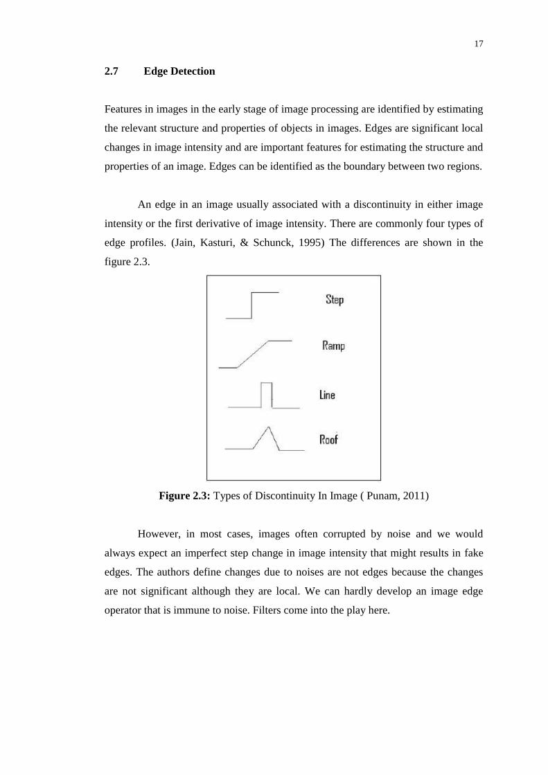
An edge in an image usually associated with a discontinuity in either image
intensity or the first derivative of image intensity. There are commonly four types of
edge profiles. (Jain, Kasturi, & Schunck, 1995) The differences are shown in the
figure 2.3.
Figure 2.3: Types of Discontinuity In Image ( Punam, 2011)
However, in most cases, images often corrupted by noise and we would
always expect an imperfect step change in image intensity that might results in fake
edges. The authors define changes due to noises are not edges because the changes
are not significant although they are local. We can hardly develop an image edge
operator that is immune to noise. Filters come into the play here.

18
2.7.1 Edge Detection Operation
In each of the operator-based edge detection strategies, the gradient magnitude is
computed in accordance with the formula given below in section 2.7.2. If the
magnitude of the gradient is higher than the threshold, then the presence of edge is
detected. This threshold value can be chosen low enough only when there is no noise
in the image, so that all true edges can be detected without miss. In noisy images,
however, the threshold selection becomes a problem and has to be changed to make
it applicable to all scenarios (Tinku & Ray, 2005).
2.7.2 Types of Edge Detection
Some of the commonly used edge detection techniques are the likes of Robert‟s
operator, Sobel operator and Canny„s Edge Detector.
The Robert‟s operator is a simple gradient operator based on 2 x 2 gradient operator.
The gradient magnitude is given by:
G[f(I,j)] = [f(i , j) – f(i+1 , j+1)] + [f(i+1 , j) – f(I , j+1)]
The convolution mask for Robert‟s operator is shown as below.
Sobel‟s operator is a 3x3 neighbourhood based gradient operator with two
kernels as shown below.
Gx Gy

19
The two masks are separately applied on the input image to yield two
gradient components in horizontal and vertical orientation respectively. (Tinku &
Ray , 2005)
Canny‟s edge detector has good noise immunity and at the same time detects
true edge points with minimum error. Canny edge detection covers three steps:
1. Maximizing the signal to noise ratio.
2. An edge localization factor, which ensures that the detected edge is localized
as accurately as possible.
3. Minimizing multiple responses to a single edge.
Maini and Aggarwal (2009) carried out a study to compare various image
edge detection techniques. They studied the most commonly used edge detection
techniques of Gradient-based and Laplacian-based edge detection using MATLAB
7.0 by applying them to different scenarios.
It was concluded that gradient-based algorithms are very sensitive to noise.
The mentioned algorithms have difficulties in distinguishing valid image contents
from visual artefacts introduced by noise. On the other hand, Laplacian-based
algorithms depend on the adjustable parameter that controls the size of Gaussian
filter. The higher the size of Gaussian‟s filter, the more blur the image gets, and some
important information could be lost. In conclusion, the authors stated that Canny‟s
edge detection performs the best under almost all scenarios compared to the others.
Thakare (2011) carried out a study in segmentation and edge detection
techniques. The main focus of this paper is to implement edge detection algotithms
to separate segments in an image. The author measures the edge detectors
performance by two scales, namely “False Acceptance Rate (FAR)” and “False
Rejection Rate (FRR)”. A test was applied to Prewitt edge detector and Sobel edge
detector. Both edge detectors outperform each other in two different images. The
outcome showed that the effectiveness of edge detectors depend on the type of image.
CHAPTER 3
3 METHODOLOGY
3.1 Operation of the Automated Tennis Ball Collector and Launcher Robot
Generally, the tennis ball collector and launcher robot is programmed into a few
subsystems. Each of those subsystems will be activated separately or simultaneously
depending on the commands received from the user and the mode of operation that
the robot is in. Robot navigation and maneuvering system controls the robot‟s motion.
The robot is able to switch operation mode whenever commanded to. The two
options of modes are ball collection system and ball launcher system.
These two modes are implemented to provide user an option to either collect
tennis balls in the court or to launch tennis balls to the user. For example, when the
Balls Collection System is activated, Object Recognition System is activated to scan
for the target objects‟ locations and export the data to Robot Navigation System
before it starts moving towards its goal. Then, when the robot is in range to capture
the balls, Balls Collection System will be activated. In Balls Launching Mode, the
robot will launch tennis balls from its storage tank to the other side of the court. The
speed and estimated end position are based on user‟s preference. The home position
of the robot will be predefined by the user.
Machine vision is integrated with the tennis Ball Collection System to
achieve a smart robotic system that gives precision and accuracy in optimizing the
balls collection task. As collection speed is concern to most users, implementing Ball

21
Recognition System provides vision to the robot in determining the objects‟ location.
This system helps to make decision on the path taken by the robot. Moreover, it helps
reduce power usage by activating Ball Collection System only when the balls are
near enough. Thus, it could help in increasing energy saving and minimize energy
waste.
3.2 System Architectural Flow Chart
The flow chart of the object recognition system operation is shown in Figure 3.1.
Figure 3.1: Automated Tennis Ball Collector and Launcher Robot Overall Flow
Chart

22
When the system is turned on, either Ball Collection Mode or Ball Launcher
Mode is chosen. If Ball Collection Mode is chosen, Ball Recognition System will
initialize and capture an image to be processed. Once the system identifies presence
of balls, it sends an array of data consisting balls location and distance to the Robot
Navigation System. Robot Navigation System will guide the robot to the target and
activates Ball Collector System. If the Ball Recognition System fails to find balls, it
sends a signal to turn the entire robot for 45 degrees and restart the process. If no
balls are found in consecutive 8 times, covered 360 degrees vision, the system will
shut down.
3.3 Properties and Parameters Selection
Selecting the right methods and configurations are very important. In this subtopic,
various options were evaluated and a final solution was selected.
3.3.1 Input Image Type Selection
Binary images are images with only two possible intensity values, which are 0 and 1.
Binary images require smaller memory requirement compared to colour images. In
other words, the small memory requirement enables faster execution time and less
computational expensive. Therefore, binary images are often used in large industrial
applications like medical imaging applications and security video cameras. However,
the drawbacks of binary images have restricted its application in certain fields.
Binary image processing is not ideal in applications which require internal
details of an image to distinguish its characteristic. Furthermore, to avoid uneven
reflection, an external lighting source such as overhead projector and light box are
used to overcome this problem, which indirectly restricting the environment. On top
of that, imperfect lighting intensity might affect the contrast of background and the

23
object. Furthermore, binary image processing cannot be extended into 3-dimensional
images; thus, losing out details for other image processing techniques.
The intensity levels determine the quality of an image, which also means,
better representation of the scene. This benefit comes with a trade-off of
computational cost and storage size. Grayscale images are digital images which carry
intensity values. They can also be synthesized from full coloured images.
In this project, high quality images are ideal to enable better recognition of
tennis balls. As tennis balls are relatively small compared to the surrounding objects
and background, high resolution images will be nice for higher range of intensity
values. Colour image is also important because one way of differentiating tennis
balls from others background objects is colour segmentation. The computational cost
and storage cost can be negligible as a laptop will be used as the processing unit of
the robot instead of microprocessor with much lower computational ability.
3.4 Image Pre-processing Techniques
Image pre-processing is an important step in image processing. In this step, relevant
features in an image are kept and the non-relevant noises are filtered out. The image
pre-processing techniques used in this projects are Gaussian Filter and Canny‟s Edge
Detector.
3.4.1 Image Filter
One of the image pre-processing techniques is the image filtering technique. Median,
Mean and Gaussian filters are two popular filtering techniques.

24
Median filter could remove salt and pepper noise and impulse noise very
effectively and in the same time retain sharp edges of the background image.
Gaussian‟s filter is particularly good in removing Gaussian‟s noise. Gaussian
noise imposes great intensity variations to an image. Since it does not have dynamic
disadvantage over the target image, Gaussian‟s filter technique will be considered in
this application.
Mean filter is rather unsuitable in this project‟s application as it removes all
the sharp edges by uniformly distributing the intensity values of an image. It causes
blur images and it is not ideal for edge detection in the later stage. Gaussian Filter
was chosen.
3.4.2 Edge Detection
Edge detection technique is a method to detect edges in an image. Edges normally
carry the boundaries information of an image. They are very important because they
represent segments and regions in an image. Before object recognition technique can
be applied on the image, edge detection is needed to find significant edges in the
image.
Canny‟s Edge Detector is more robust than the other edge detection
techniques in identifying false edges. There is a risk if the system detects fake edges
and may mislead the robot to a wrong location where there is no desired objects.
Moreover, Canny‟s Edge detector has good noise immunity and at the same
time detects true edge points with minimum error.
Sobel‟s Edge detector is less suitable compared to Canny‟s Edge detector
because it produces much wearker edge outlines. Strong edge outlines is a important

25
factor where it may affect the accuracy of shape recognition technique in the latter
stage and thus, some objects may be missed out. Canny‟s Edge Detector was chosen.
3.5 Object Recognition
One of the circle recognition techniques that could be implemented in this project is
the Hough Transform. Hough Transform is the most popular and is one of the most
effective feature extraction techniques. The most obvious feature of the object in this
project is the circular shape of the tennis ball.
Hough transform was chosen as the object recognition technique that to be
developed in for some of its advantages. Hough Transform circle detection can detect
multiple instances of model in a frame. This feature makes Hough Transform the
most robust method in recognizing multiple tennis balls in one frame.
The robustness of Hough Transform is further supported by its operation. The
voting mechanism as described earlier is very unlikely to be sensitive to noise. The
reason behind this is that the noise points are unlikely to contribute consistently to
any single bin. Therefore, noise points can hardly characterize a false circle.
However, if compared to another possible object recognition technique called
colour segmentation, Hough Transform has the disadvantage of higher computational
time. The reason is because Hough Transform will need to undergo much iteration to
find the circle characteristic, and thus may have higher misses and false repeats.
On the other hand, Colour segmentation is a technique that classifies objects
by comparing the colour space of the objects. The three parameters are luminance, Y,
hue, I and saturation, Q. Although Hough Transform is robust in finding shapes,
Colour segmentation is still a better option considering various objects‟ intensity
values in various lighting and weather scenarios that could add on to the noises of an
image. Colour segmentation was used to achieve the objectives.

26
3.6 Objects Location Mapping
Objects‟ location will be determined by the centroids. Centroid is the center point of
a group of white pixels. The values are in term of x- and y-coordinate. A marker is
plotted in the original image.
Once the centroids are found, the locations of the tennis balls can be
determined by implementing mathematical algorithm. The x- and y-coordinates
values are divided by the respective range of each axis. The outcome values are
corresponding with the regions of existence of tennis balls.
3.7 Program Overview
Firstly, yellow colour is extracted from the image. The extracted image is then
converted into gray scale image before applying a suitable threshold value. The final
outcome will be in binary image which only consists of black and white pixels. The
pixels representation for white pixels is „1‟ and for black pixels is „0‟.
After that, properties like area, size and eccentricity are introduced to define the
groups of pixels that representing the balls. The proposed Hough Transform was not
used because of overwhelming noise in our application. Please see Chapter 4 for
results and discussion.
3.8 Matlab
Matlab was chosen to develop the ball recognition because it has many advantages
over the other image processing software. Firstly, Matlab in full is called the „Matrix
Laboratory‟. It is a programming environment for algorithm development, data
analysis, visualization, and numerical computation. Matlab is fast in debugging code
and the mathematical command syntax is much simple. Most importantly, it has the

27
capability of extracting variables‟ information in a workspace. For example, the
information like „size‟, „bytes‟, „class‟, „attributes‟ are useful to know what‟s going
on with the program. In other words, pixels information is stored in a matrix format
in the workspace after each processing steps.
Matlab toolboxes provide a comprehensive set of reference-standard
algorithms and graphical tools for all engineering and technical simulations. The
toolboxes used in this project are the Image Processing Toolbox and Image
Acquisition Toolbox.
3.9 Software Development and Implementation
In this section, the software that was used to develop and implement the tennis ball
recognition system will be discussed in detail. Matlab was used with webcam to
perform ball recognition tasks. Visual Basics Studio was used to program the
computer integrate card, IFC-CI00. The function of the computer interface card is to
control motor driver boards to perform tasks when prompted to.
3.9.1 Image processing Toolbox
Image Processing Toolbox provides a comprehensive set of reference-standard
algorithms and graphical tools for image processing, analysis, visualization, and
algorithm development.
Image Processing Toolbox interestingly allows user to explore an image,
examine a region of pixels, adjust the contrast, create contours or histograms, and
manipulate regions of interest (ROIs). With toolbox algorithms user can restore
degraded images, detect and measure features, analyze shapes and textures, and
adjust colour balance and more (Mathworks, 1994).

28
3.9.2 Image Acquisition Toolbox
Image Acquisition Toolbox enables user to acquire images and video from cameras
and frame grabbers directly into MATLAB workspace. Advanced workflows could
trigger acquisition while processing in-the-loop, perform background acquisition,
and synchronize sampling across several multimodal devices (Mathworks, 1994).
3.10 Image Acquisition System
Logitech HD webcam C270h is used as the frame grabber in this project. The
sequence to capture an image from the frame grabber into Matlab workspace is as
follows:
i. Start up webcam preview video
ii. Retrieve a frame from the preview video
iii. Write the image file into computer‟s hard disk
iv. Read image file from computer‟s hard disk
The code of the above mentioned sequence is as follows:
vid = videoinput('winvideo', 1, 'RGB24_1280x960'); start(vid); wait(vid);
snapshot = getsnapshot(vid); imwrite(snapshot,'test.jpg','jpg')
tennis1 = imread('test.jpg'); imagesc(tennis1);
The video input is configured to be colour image in RGB plane of 1280x960
pixels. Matlab will return a frame as the file name „snapshot‟ before writing it to
computer‟s hard disk as „test.jpg‟. Matlab then reads the image data and store the
information into variable name „tennis1‟. „imagesc‟ is a command to display variable
„tennis1‟ as a picture.

29
3.11 Colour Planes Extraction
A full colour image captured by the webcam can be viewed as a 3D matrix consisting
3 2D colour planes. These 2D planes consist of data corresponding to the red, green
and blue components of the image. The combinations of these three colours produce
different colours. In this step, „Indexing‟ was done to extract the three colour planes
from the 3D matrix.
r = tennis1(:, :, 1); g = tennis1(:, :, 2); b = tennis1(:, :, 3);
Where,
r represents red plane
g represents green plane
b represents blue plane
A(:,:,k) is the kth page of three-dimensional array A.
Since yellow colour is the combination of the intensity values on r,g and b
planes, a arithmetic operation on the matrices as a whole was performed to try to
create one matrix that represents an intensity of yellow.
3.12 Threshold the Image
A threshold value was set to separate the parts of an image that considered as yellow
from the rest. The image was returned in binary image. Many samples of cropped
tennis balls from the image were calculated using „bwarea‟ and „boundingbox‟
command to identify the range of area and eccentricity the tennis balls would fall
into. The threshold value was set to 230.

30
3.13 Find Objects’ Region Properties
The objects that fall into the defined area and eccentricity range are considered as
tennis balls. „Area‟ is defined as the number of white pixels contained in an object.
Eccentricity is a measure of how much the shape of the perimeter differs from a
perfect circle. Bounding box is a function that encloses objects with a box.
Eccentricity was used with bounding box to predict the shape of tennis ball. In short,
the information from the combination of these two functions is similar to the ratio of
major axis over minor axis.
3.14 Systems Integration
The individual systems of the robot will be integrated using Interface Free Controller,
IFC. A main board will act as a main controller connecting computer and all the
motor driver cards used in the robot. The main board, also known as the computer
interface card, is programmed using Visual Basic. It has the responsibility to send
and receive signals to and from computer to automate the robot to complete its tasks.
The tennis ball‟s positions found from the Ball Recognition System are sent
to Visual Basic environment to process the robot‟s navigation. After the tennis balls
found in the image are successfully collected, the Robot Navigation System has to
send a signal to notify the Ball recognition System to restart the program, when the
robot is not moving. This repeats until the robot finishes collecting all the tennis balls.
To do that, Matlab has to be compatible with Visual Basic and vice versa.

CHAPTER 4
4 RESULTS AND DISCUSSIONS
4.1 Introduction
Simulations were conducted on some of the image processing techniques and the
results are shown and discussed in this section. The simulations were done using
MATLAB.
4.2 Image Acquisition System Design Parameters
Image acquisition is an important step in image processing because the quality of
image has direct effect to the outcome. During the first attempt, the input video
resolution was set to a low resolution (640 x 480), hoping to reduce the processing
time of getting a snapshot from the video frames. However, the final outcome of the
image processing was bad due to the low colour resolution and poor sharpness of the
image. Dealing with far and wide landscape like a tennis court is more ideal to have a
higher resolution image. Moreover, higher resolution of the video input only affects
the image acquiring time by a little amount of delay. Figure 4.1 and 4.2 show the
comparison of time taken to retrieve one frame from two different resolution video.

32
Figure 4.1: Time to retrieve an image from a 640 x 480 video is 3.2249 seconds
Figure 4.2: Time to retrieve an image from a 1280x960 video is 3.3921 seconds
33
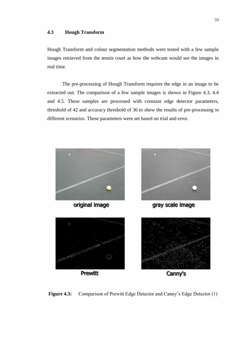
4.3 Hough Transform
Hough Transform and colour segmentation methods were tested with a few sample
images retrieved from the tennis court as how the webcam would see the images in
real time.
The pre-processing of Hough Transform requires the edge in an image to be
extracted out. The comparison of a few sample images is shown in Figure 4.3, 4.4
and 4.5. These samples are processed with constant edge detector parameters,
threshold of 42 and accuracy threshold of 36 to show the results of pre-processing in
different scenarios. These parameters were set based on trial and error.
Figure 4.3: Comparison of Prewitt Edge Detector and Canny‟s Edge Detector (1)

34
Canny‟s Edge Detector could detect more detailed edge than Prewitt Edge
Detector. The edge of tennis ball is successfully extracted out using both edge
detectors.
Figure 4.4: Comparison of Prewitt Edge Detector and Canny‟s Edge Detector (2)
Figure 4.4 shows the image with a tennis ball located in front of the fence.
The result shows that both edge detectors are not capable of filtering out the noise in
the area where the edge has the similar colour. From the grayscale image it is seen
that the part where the grass and fence overlap has poor and weak edge.
35
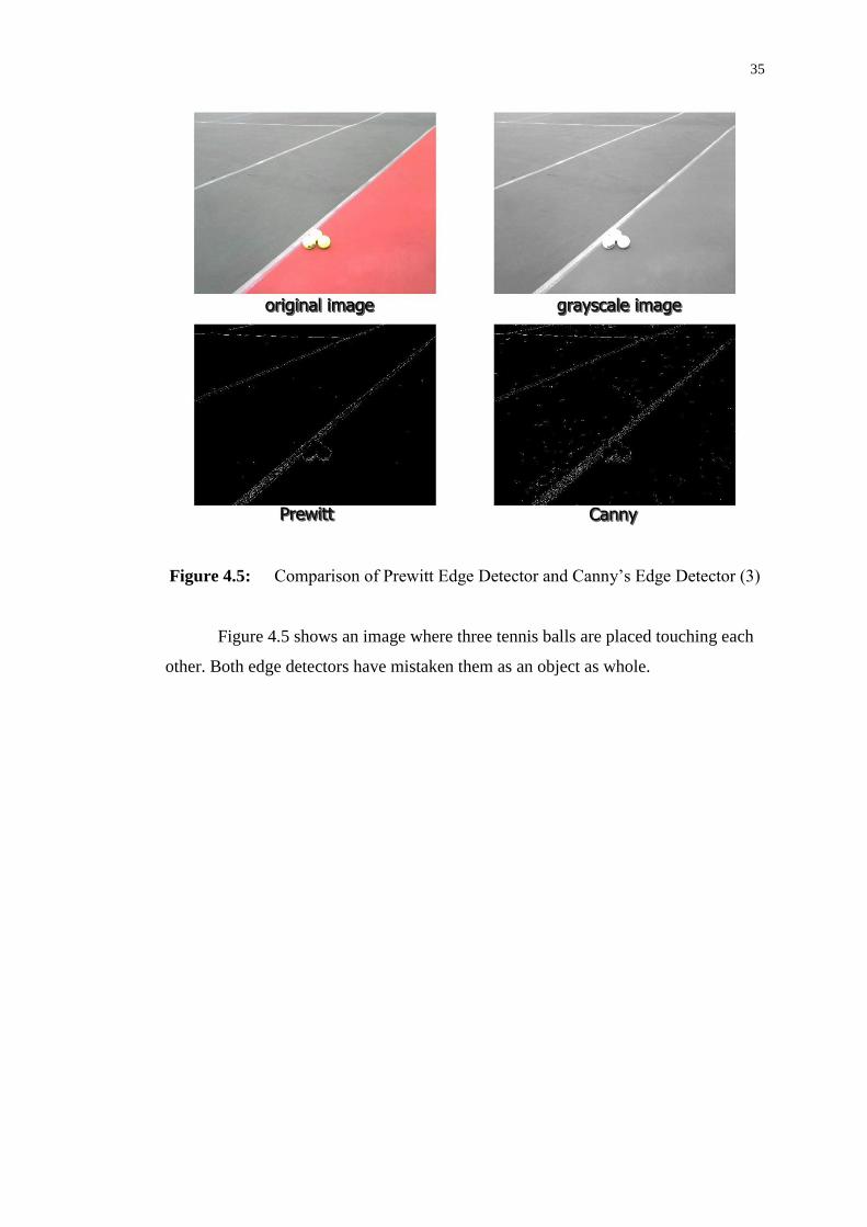
Figure 4.5: Comparison of Prewitt Edge Detector and Canny‟s Edge Detector (3)
Figure 4.5 shows an image where three tennis balls are placed touching each
other. Both edge detectors have mistaken them as an object as whole.

36
4.3.1 Hough Transform Outcome
Figure 4.6: Hough Transform based on result in Figure 4.3
The simulation is done with the result from the Canny‟s Edge Detector in
Figure 4.3. It is observed that the Hough Transform failed to detect the tennis ball
and mistaken other objects as circles. One of the main reason is the contour of the
image is not good enough to extract the tennis ball in full circle shape. The Hough
Transform could not detect any circles using Prewitt Edge Detector.

37
Figure 4.7: Hough Transform based on result in Figure 4.4
The simulation is also done with the result from the Canny‟s Edge Detector in
Figure 4.4. The outcome seems bad because it detects false circles even with
maximum threshold for both images.
As for Hough Transform application in the outcome in Figure 4.5, no circles
were detected in both images. The reason could be there are no significant circular
shapes in those images.
From the simulation discussed, it is confirmed that Hough Transform is not
the method we want to use to meet our objectives. The contour of the image is not
obvious and might change depend on the weather. When the sun is too bright, some
parts in the colour image will become too bright and thus might not be considered as
outline/edge in the edge detection process. Finally, circular shapes are difficult to
detect.
4.4 Colour Segmentation
Another method that could be used to perform similar function to extract circular
shapes from images is the colour segmentation method. Like Hough Transform,
colour segmentation processes the images in grayscale format. The difference here is
the specific colour planes are used to perform segmentation rather than the original
colour image. Colour planes can be mathematically re-defined and thus, helps
38
segment colour planes more efficiently. For example, a pure red, green or blue colour
can be segmented out from a full colour image using colour segmentation technique.
This section shows the results of colour segmentation in the effort to find
tennis balls in an image. After the colour images are extracted to its basic colour
planes, which are red, green and blue, a mathematic equation was introduced to
further define a colour plane for yellow. Yellow colour plane is a plane where the
yellow colour intensity is extracted from the image. Therefore, tennis balls and any
other yellow colour objects would appear as white pixels in yellow colour plane.
Equation 4.1 was developed to define yellow colour plane.
(4.1)
Where,
yellow = variable for yellow colour plane
r = variable for red colour plane
g = variable for green colour plane
b = variable for blue colour plane
39
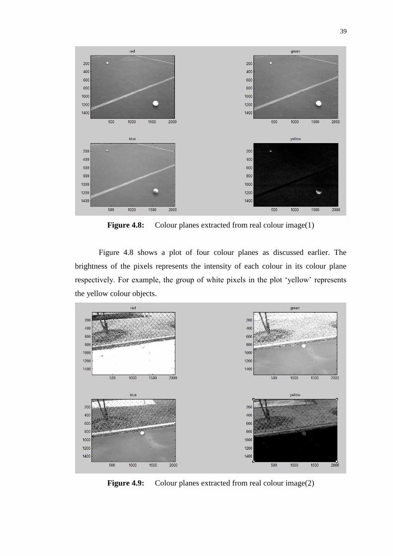
Figure 4.8: Colour planes extracted from real colour image(1)
Figure 4.8 shows a plot of four colour planes as discussed earlier. The
brightness of the pixels represents the intensity of each colour in its colour plane
respectively. For example, the group of white pixels in the plot „yellow‟ represents
the yellow colour objects.
Figure 4.9: Colour planes extracted from real colour image(2)

40
Figure 4.10: Colour planes extracted from real colour image(2)
Figure 4.8 – 4.10 show that the equation is workable and yellow colour
objects can be extracted out from the image. This helps a lot in filtering out the
background. Further circle detection techniques will help us find the tennis balls.
4.5 Threshold Values
As discussed in Chapter 3.9, thresholding is a binarization method that converts
grayscale images into binary images, which its binary bit classification is determined
by the threshold value. In normal scenarios, objects are represented by the brighter
pixels in a grayscale image, and „1‟ pixel (white) in binary images.
Referring to the simulation in section 4.4, not all white pixels are the objects
that we want. Some pixels might be formed by other yellow colour objects that are
not tennis balls.

41
Figure 4.11: Yellow plane image with different threshold values (1)
In binary thresholding, threshold values of 100 means that any pixels that has
intensity values above 100 are considered as objects (white pixels) and so on. Figure
4.11 shows that the higher the threshold values, the more accurate it is to remain the
yellow intensity pixels.

42
Figure 4.12: Yellow plane image with different threshold values (2)
Figure 4.12 points out the drawback of object recognition using only colour
segmentation. It shows that even with the maximum threshold values of 254 (each
pixel has 255 intensity levels), the image might still have some of the non relevant
objects. As for the right bottom picture in Figure 4.12, the non relevant objects are
referred to the white pixels located above the round objects.

43
4.6 Determining threshold values
Figure 4.13: Yellow plane image with different threshold values (3)
Figure 4.13 points out another drawback of colour segmentation. If the
objects overlap each other, the system could not recognize them as individual objects.
Hough Transform on the other hand, has the advantage of recognizing overlapped
objects.
From the colour segmentation and thresholding operation, it was shown that
the Ball Recognition System cannot rely on just colour segmentation as a lone
method. Therefore, other properties of a tennis ball must be examined and relate
them as a fulfilment to define an object as a tennis ball. The further improvement of
the Ball Recognition System using region properties is discussed in section 4.7.
44
4.7 Region Properties Measurement
The measurement of region properties is useful in finding a target based on the
properties in a part of matrix. The region properties implemented in this project were
the area, bounding box, eccentricity and centroid.
4.7.1 Area
„Area‟ is the actual number of pixels in the region. Using this property, area of a
tennis ball is found to be in the range of 1600 pixels and 13000 pixels. Since
thresholding may eats up more pixels than it should, aking a 10% allowance for these
values is reasonable. The range is set to be 1500 pixels and 14500 pixels.
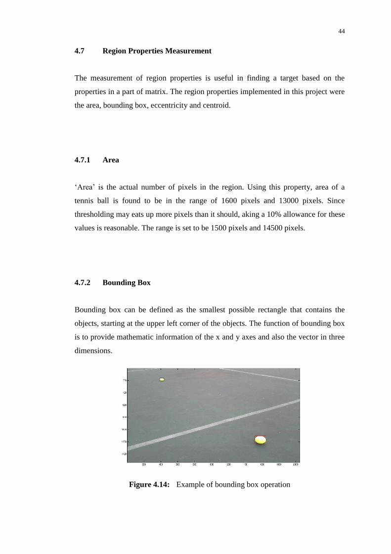
4.7.2 Bounding Box
Bounding box can be defined as the smallest possible rectangle that contains the
objects, starting at the upper left corner of the objects. The function of bounding box
is to provide mathematic information of the x and y axes and also the vector in three
dimensions.
Figure 4.14: Example of bounding box operation

45
4.7.3 Eccentricity
Eccentricity is the ratio of major axis over minor axis. It is most used in finding ratio
of an ellipse. Circle is considered as a special kind of ellipse. Eccentricity value is
ranged from 0 to 1. It can be thought of as a measure of how much the conic section
deviates from being circular.
Figure 4.15: Example of eccentricity operation
Figure 4.15 shows the process of applying bounding box and eccentricity.
Only the objects that meet the conditions of bounding box and eccentricity will be
boxed.

46
4.7.4 Centroid
In geometry, centroid of an area is the center of mass of a body. For illustration, the
distance from x-axes to centroid is Cx, and the distance from y-axes to centroid is Cy.
The coordinates of centroid is (Cx, Cy).
Figure 4.16: Example of centroid operation
Figure 4.16 shows centroids are found from each of the objects and plotted on
the figure. Values of the ball locations are returned to a variable and displayed to the
user.

47
Figure 4.17: Example of centroid operation with and without region properties

48
The results from Figure 4.17 compare the outcome of Ball Recognition
System with and without considering region properties. The upper picture shows that
many false objects have been detected. Most of the false objects are located outside
the tennis court, which is the grass area. This is because the grass colour is very
similar to the colour of yellow. After redefined the search with region properties, the
accuracy is much improved.
4.8 Final results
It was finalized that the Ball Recognition System to have a system design parameters
as in Table 4.1.
Table 4.1: Ball Recognition Design Parameters
System Parameters Values
Binary Threshold 230
Region Area 1500-145000 px
Eccentricity < 0.85
Finally, the Ball Recognition System was successful implemented. All tennis
balls were successfully detected and 90% of the false objects were successfully
filtered. Moreover, the Ball Recognition System is able to detect multiple tennis balls
in one program cycle.

49
Figure 4.18: Ball Recognition System
Figure 4.18 shows an example of Ball Recognition System in different
scenarios. The picture on the top left corner shows that the Ball Recognition System
is able to detect multiple tennis balls in the same time not mistaken the tennis court
lines as an object. The picture on its right shows that the tennis balls could be
differentiated from other shapes. The bottom left picture shows that if the camera
angle is placed too high or the tennis ball is located too far from the system, it might
be mistaken as non-object because of its size. The last picture proved that the system
could recognize a group of tennis balls sticking onto each other.
4.9 Finding Tennis Balls’ Location
The location of tennis balls are calculated using ratio of the actual distance to the
coordinate system of the Ball Recognition System. The actual distance is measured
from the frame grabber to the centre of tennis balls. The actual distance measured

50
along the bottom and top x-axes of the webcam facing 30 degree downwards was
70cm and 72cm respectively. The distance along the y axes was measure 368cm on
average. The accuracy of the distance is ±5cm. These errors are considered very
small and negligible because the opening of the Ball Collection System is wide
enough to overcome 30cm of error.
4.10 Problems Encountered
There are several problems that occur in the development of the Ball Recognition
System. The problems faced in the image processing are the false objects and the
presence of obstacle. Time consumption of the whole process is also a concern to
decide whether the robot should run the Ball Recognition System continuously or by
signal triggered.
4.10.1 False Objects Detection
False objects always confuse the system to identity them as tennis balls. These false
objects have almost same shape geometries and colour as the tennis balls. The author
tried to use the colour segmentation together with Hough Transform to create a better
Ball Recognition System but it is quite a challenge to perform Hough Transform on
binary images as the outcome of colour segmentation is in the binary image format.

51
Figure 4.19: White colour objects mistaken as objects by the system
The white colour spots behind the net are mistaken as objects because the
colour intensity level is very close to yellow colour intensity level. The ratio of major
axes to the minor axes also falls in the range of tennis balls‟ eccentricity property.
Another problem faced is the colour of the sky. Similarly, anything outside
the constraint and the sunlight might be mistaken as objects too.
To overcome this problem, the camera angle has to be 30 degree downwards
to avoid sunlight appearing in the system‟s vision.
4.10.2 Presence of Obstacles
Besides, if a real tennis balls are detected behind the net, the robot must navigate
itself around the obstacle to reach to the balls. One difficulty faced here is the

52
recognition of obstacle. It requires a lot of time to develop an Obstacles Avoidance
System. Moreover, the net is difficult to detect under different weather and sunlight
intensity as the edges are not significant to the image processing system.
Figure 4.20: Sky mistaken as objects by the system
53
4.10.3 Time Consumption
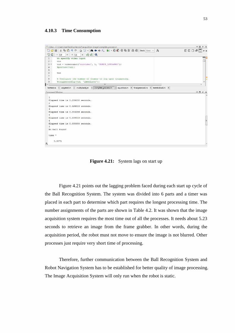
Figure 4.21: System lags on start up
Figure 4.21 points out the lagging problem faced during each start up cycle of
the Ball Recognition System. The system was divided into 6 parts and a timer was
placed in each part to determine which part requires the longest processing time. The
number assignments of the parts are shown in Table 4.2. It was shown that the image
acquisition system requires the most time out of all the processes. It needs about 5.23
seconds to retrieve an image from the frame grabber. In other words, during the
acquisition period, the robot must not move to ensure the image is not blurred. Other
processes just require very short time of processing.
Therefore, further communication between the Ball Recognition System and
Robot Navigation System has to be established for better quality of image processing.
The Image Acquisition System will only run when the robot is static.

54
Table 4.2: Number Assignment to Image Processing Processes
Processes Information Number Assignment
Start up preview video and acquire an
image and store in system‟s hard disk
1
Read the acquired image from hard disk
into MATLAB workspace
2
Extract red, green, blue colour planes 3
Perform arithmetic calculation to obtain
yellow colour plane and plot those colour
planes
4
Threshold the yellow colour planes to
extract yellow colour objects
5
Find relevant region properties to locate
tennis balls
6
4.10.4 System Integration
When image processing is done using Matlab, the data array defining the locations of
the tennis balls (if found) must be exported into Visual Basics to perform
corresponding commands. The problem faced was the complexity of outputting data
from Matlab to Visual Basics. Both programs must run simultaneously in a loop to
ensure a smooth operation.
Other than that, the serial communication, UART was tested to be unstable at
times. The USB to UART converter was initially tested with HyperTerminal
program. The „receive‟ and „transmit‟ pins were shorted and it gave an unstable
response when data was sent. This may because of hardware problems and
undiscovered technical issues.

CHAPTER 5
CONCLUSIONS AND RECOMMENDATIONS
5.1 Conclusions
The project was finally completed after 6 months of hard work and determination
from the team. All the objectives were met and the expected tasks were successfully
accomplished.
In Chapter 2, all the existing technologies on image processing and circular
objects recognition were discussed. The literature review topics include the
fundamental of image, object recognition techniques, image filtering and edge
detection Techniques. The existing technology was useful in helping the
understanding and ideas generation throughout this project.
The first objective is to design and develop a ball recognition system. The
author shows the methodology and techniques implementation in Chapter 3. The
detailed implementation is shown starting from the operation of the robot, general
flow chart and the software development. The software development stages were the
input image selection, Hough Transform, colour segmentation and finally, system
integration. A successful Ball Recognition System was done in the end.
The second objective is to be able to identify ball objects. The Ball
Recognition System developed in this project is capable of identifying tennis balls

56
and differentiate them from most of the background objects. The technique to
achieve this is by implementing the colour segmentation and finding the various
region properties of a tennis ball.
The last objective is to be able to determine the ball location correctly and
accurately. This objective is achieved by finding the centroid, center mass of the
tennis balls. The distance is the detected tennis balls are calculated using the ratio of
actual distance and the number of pixels displayed in the image‟s coordinate system.
Matlab was the main program to develop this project. The author has
acquired much knowledge in using this program, especially in matrix operation and
graph plotting. Besides, the author has also familiar with the programming syntax
and command language used in Matlab.
Developing a real time tennis balls recognition system is never an easy task.
There were many problems popped out during the project duration, but with the help
of Dr Tan, lecturers and team mates, the problems were solved.
In conclusion, the author has gained priceless experience and knowledge in
technical terms and project management. These skills provided the author a strong
platform in future career.
5.2 Recommendations
There are a lot of rooms for improvement in this project. The time and budget
constraint of this project had limited the performance of the robot.
Firstly, the improvement can be done to detect tennis balls more accurately
and effectively is to introduce a shape detection algorithm. As discussed in Chapter 4,
the current Ball Recognition Program could still mistaken some of the background
objects as tennis balls. With the introduction of shape detection, the Ball Recognition

57
System does not only rely on finding colour, area, eccentricity of the objects, but also
the shape geometry of the objects. This will surely improve the accuracy and success
rate of the system.
Secondly, obstacles avoidance using machine vision and artificial intelligence
is preferable to improve the robot‟s capability. With obstacles avoidance and
intelligent path planning, the robot can fully replace human in collecting the tennis
balls. Furthermore, the robot could navigates itself around everywhere in the tennis
court to complete its task.
Last but not least, the systems integration must be improvised to give a more
stable integrated system to achieve better results. Matlab and Visual Basics should
have made compatible and user friendly to ease data sharing and establish a more
robust signalling system. Other than that, artificial intelligence like neural network
and fuzzy logic can be used to perform path planning in the future.
It would be essential that improvements are made from time to time to ensure
its place in the competitive market nowadays in sports automation.

58
REFERENCES
A. Ahmadyfard, J. Kittler (2002). A Comparative Study of Two Object Recogintion
Methods
Jinzi Mao (2006). Tracking A Tennis Ball Using Image Processing Techniques
Heung .S. K, Jong-Hwan.K (2000). A Two Step Circle Detection Algorithm From
The Intersecting Chord. Elsevier.
R. Jain, R. Kasturi, & B. Schunck, (1995). Machine Vision. McGraw-Hill Inc
L. Vandevenne (2004). Image Filtering. Retrieved July 5, 2011, from
http://lodev.org/cgtutor/filtering.html
Raman Maini, Himanshu Aggarwal (2002). Study and Comparison of Various Edge
Detection Techniques. International Journal of Image Processing (IJIP), Volume (3) :
Issue (1)
Punam Thakare (2011). A Study of Image Segmentation and Edge Detection
Techniques. International Journal on Computer Science and Engineering (IJCSE);
ISSN : 0975-3397
(2000) Lossless Coding of Bi-level Images, ISO/IEC 14492-1
Tinku Acharya, Ajoy K.Ray (2005). Image Processing Principles and
Applications.John Wiley & Sons,inc.,Publication

59
Maria Petrou, Panagiota Bosdogianni (1999). Image Processing The Fundamentals.
John Wiley & Sons,inc.,Publication
Ibrahim A. Hameed, Claus G. Sorrenson, Dionysis Bochtis, Ole Green (2011). Field
robotics in sports: automatic generation of guidance lines for automatic grass
cutting, striping and pitch marking of football playing fields. International Journal of
Advanced Robotic Systems, Vol. 8, No. 1 ISSN 1729-8806, pp 113-121
Andre Senior, Sabri Tosunoglu (2005). Hybrid Machine Vision Control. Florida
Conference on Recent Advances in Robotics
Q. Ji, Y.Xie (2003). Randomised Hough Transfrom With Error Propagation For
Line And Circle Detection. Springer-Verlag London Limited
Ali Ajdari Rad, Karim Faez, Navid Qaragozlou (2003). Fast Circle Detection Using
Gradient Pair Vectors.

60
APPENDICES
APPENDIX A: Matlab Source Code
%% specify video input tic vid = videoinput('winvideo', 1, 'RGB24_1280x960');
start(vid); wait(vid);
%% while true
snapshot = getsnapshot(vid); imwrite(snapshot,'test.jpg','jpg')
%% Read in Image
tennis1 = imread('tennis2.jpg'); imagesc(tennis1);
%% Extract each color
r = tennis1(:, :, 1); g = tennis1(:, :, 2); b = tennis1(:, :, 3);
yellow = g - (r/2) - (b/2); Plotcolors(r, g, b, yellow);
%% Close plotcolors close
%% Threshold the image
bw = g > 230; bwarea(bw); %compute area in objects colormap(gray);

61
%% Identify all objects
disp('5'); s = regionprops(bw,
{'centroid','area','BoundingBox','Eccentricity'});
if isempty(s) disp('No ball found!'); else id = find([s.Area] > 300 & [s.Area] < 100000 & [s.Eccentricity]
< 0.7);
if length(id) < 1 disp('No ball found!'); else
dist = [];
for ii = 1:length(id);
disp('ball found!');
hold on
plot(s(id(ii)).Centroid(1),s(id(ii)).Centroid(2),'wp','MarkerSize',1
0,'MarkerFaceColor','r'); rectangle('Position', s(id(ii)).BoundingBox, 'EdgeColor', 'r'); hold off
if s(id(ii)).Centroid(1)<=320 &
s(id(ii)).Centroid(2)<=240 disp('region 1'); elseif s(id(ii)).Centroid(1)> 320 &
s(id(ii)).Centroid(1) <= 640 & s(id(ii)).Centroid(2) <=240 disp('region 2'); elseif s(id(ii)).Centroid(1)> 640 &
s(id(ii)).Centroid(1) <= 960 & s(id(ii)).Centroid(2) <=240 disp('region 3'); elseif s(id(ii)).Centroid(1)> 960 &
s(id(ii)).Centroid(2)<=240 disp('region 4');
elseif s(id(ii)).Centroid(1)<=320 &
s(id(ii)).Centroid(2)> 240 & s(id(ii)).Centroid(2)<=480 disp('region 5'); elseif s(id(ii)).Centroid(1)> 320 &
s(id(ii)).Centroid(1) <= 640 & s(id(ii)).Centroid(2)> 240 &
s(id(ii)).Centroid(2) <= 480 disp('region 6'); elseif s(id(ii)).Centroid(1)> 640 &
s(id(ii)).Centroid(1) <= 960 & s(id(ii)).Centroid(2)> 240 &
s(id(ii)).Centroid(2) <= 480 disp('region 7'); elseif s(id(ii)).Centroid(1)> 960 &
s(id(ii)).Centroid(2) > 240 & s(id(ii)).Centroid(2) <= 480 disp('region 8');

62
elseif s(id(ii)).Centroid(1)<=320 &
s(id(ii)).Centroid(2)> 480 & s(id(ii)).Centroid(2)<=960 disp('region 9'); elseif s(id(ii)).Centroid(1)> 320 &
s(id(ii)).Centroid(1) <= 640 & s(id(ii)).Centroid(2)> 480 &
s(id(ii)).Centroid(2) <= 960 disp('region 10'); elseif s(id(ii)).Centroid(1)> 640 &
s(id(ii)).Centroid(1) <= 960 & s(id(ii)).Centroid(2)> 480 &
s(id(ii)).Centroid(2) <= 960 disp('region 11'); elseif s(id(ii)).Centroid(1)> 960 &
s(id(ii)).Centroid(2) > 480 & s(id(ii)).Centroid(2) <= 960 disp('region 12');
elseif s(id(ii)).Centroid(1)<=320 disp('region 13'); elseif s(id(ii)).Centroid(1)> 320 &
s(id(ii)).Centroid(1) <= 640 disp('region 14'); elseif s(id(ii)).Centroid(1)> 640 &
s(id(ii)).Centroid(1) <= 960 disp('region 15'); elseif s(id(ii)).Centroid(1)> 960 disp('region 16'); end
ax(ii) = s(id(ii)).Centroid(1); by(ii) = s(id(ii)).Centroid(2); cenText = strcat('Center location is (',num2str(ax(ii),4),',
',num2str(by(ii),4),')'); disp(cenText);
dist_value = abs(s(id(ii)).Centroid(1)-640) +
abs(s(id(ii)).Centroid(2)-960); dist = [dist dist_value]; end
[min_value, position_dist] = min(dist); disp (strcat('distance from robot:', num2str(min_value)));
cenText =
strcat('Centroid:(',num2str(s(id(position_dist)).Centroid(1),4),',
',num2str(s(id(position_dist)).Centroid(2),4),')'); disp(cenText); end
end
end

63
APPENDIX B: Code of plotting colour planes
function Plotcolors(red, green, blue, yellow) %CREATEFIGURE1(red,green,blue,yellow) % red: image cdata % green: image cdata % blue: image cdata % yellow: image cdata
% Auto-generated by MATLAB on 03-Nov-2011 12:24:23
% Create figure figure1 = figure('Name','red',... 'Colormap',[0 0 0;0.0158730167895556 0.0158730167895556
0.0158730167895556;0.0317460335791111 0.0317460335791111
0.0317460335791111;0.0476190485060215 0.0476190485060215
0.0476190485060215;0.0634920671582222 0.0634920671582222
0.0634920671582222;0.0793650820851326 0.0793650820851326
0.0793650820851326;0.095238097012043 0.095238097012043
0.095238097012043;0.111111111938953 0.111111111938953
0.111111111938953;0.126984134316444 0.126984134316444
0.126984134316444;0.142857149243355 0.142857149243355
0.142857149243355;0.158730164170265 0.158730164170265
0.158730164170265;0.174603179097176 0.174603179097176
0.174603179097176;0.190476194024086 0.190476194024086
0.190476194024086;0.206349208950996 0.206349208950996
0.206349208950996;0.222222223877907 0.222222223877907
0.222222223877907;0.238095238804817 0.238095238804817
0.238095238804817;0.253968268632889 0.253968268632889
0.253968268632889;0.269841283559799 0.269841283559799
0.269841283559799;0.28571429848671 0.28571429848671
0.28571429848671;0.30158731341362 0.30158731341362
0.30158731341362;0.31746032834053 0.31746032834053
0.31746032834053;0.333333343267441 0.333333343267441
0.333333343267441;0.349206358194351 0.349206358194351
0.349206358194351;0.365079373121262 0.365079373121262
0.365079373121262;0.380952388048172 0.380952388048172
0.380952388048172;0.396825402975082 0.396825402975082
0.396825402975082;0.412698417901993 0.412698417901993
0.412698417901993;0.428571432828903 0.428571432828903
0.428571432828903;0.444444447755814 0.444444447755814
0.444444447755814;0.460317462682724 0.460317462682724
0.460317462682724;0.476190477609634 0.476190477609634
0.476190477609634;0.492063492536545 0.492063492536545
0.492063492536545;0.507936537265778 0.507936537265778
0.507936537265778;0.523809552192688 0.523809552192688
0.523809552192688;0.539682567119598 0.539682567119598
0.539682567119598;0.555555582046509 0.555555582046509
0.555555582046509;0.571428596973419 0.571428596973419
0.571428596973419;0.58730161190033 0.58730161190033
0.58730161190033;0.60317462682724 0.60317462682724
0.60317462682724;0.61904764175415 0.61904764175415
0.61904764175415;0.634920656681061 0.634920656681061
0.634920656681061;0.650793671607971 0.650793671607971
0.650793671607971;0.666666686534882 0.666666686534882
0.666666686534882;0.682539701461792 0.682539701461792
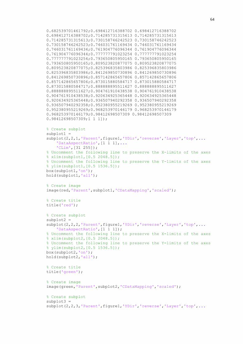
64
0.682539701461792;0.698412716388702 0.698412716388702
0.698412716388702;0.714285731315613 0.714285731315613
0.714285731315613;0.730158746242523 0.730158746242523
0.730158746242523;0.746031761169434 0.746031761169434
0.746031761169434;0.761904776096344 0.761904776096344
0.761904776096344;0.777777791023254 0.777777791023254
0.777777791023254;0.793650805950165 0.793650805950165
0.793650805950165;0.809523820877075 0.809523820877075
0.809523820877075;0.825396835803986 0.825396835803986
0.825396835803986;0.841269850730896 0.841269850730896
0.841269850730896;0.857142865657806 0.857142865657806
0.857142865657806;0.873015880584717 0.873015880584717
0.873015880584717;0.888888895511627 0.888888895511627
0.888888895511627;0.904761910438538 0.904761910438538
0.904761910438538;0.920634925365448 0.920634925365448
0.920634925365448;0.936507940292358 0.936507940292358
0.936507940292358;0.952380955219269 0.952380955219269
0.952380955219269;0.968253970146179 0.968253970146179
0.968253970146179;0.98412698507309 0.98412698507309
0.98412698507309;1 1 1]);
% Create subplot subplot1 =
subplot(2,2,1,'Parent',figure1,'YDir','reverse','Layer','top',... 'DataAspectRatio',[1 1 1],... 'CLim',[31 255]); % Uncomment the following line to preserve the X-limits of the axes % xlim(subplot1,[0.5 2048.5]); % Uncomment the following line to preserve the Y-limits of the axes % ylim(subplot1,[0.5 1536.5]); box(subplot1,'on'); hold(subplot1,'all');
% Create image image(red,'Parent',subplot1,'CDataMapping','scaled');
% Create title title('red');
% Create subplot subplot2 =
subplot(2,2,2,'Parent',figure1,'YDir','reverse','Layer','top',... 'DataAspectRatio',[1 1 1]); % Uncomment the following line to preserve the X-limits of the axes % xlim(subplot2,[0.5 2048.5]); % Uncomment the following line to preserve the Y-limits of the axes % ylim(subplot2,[0.5 1536.5]); box(subplot2,'on'); hold(subplot2,'all');
% Create title title('green');
% Create image image(green,'Parent',subplot2,'CDataMapping','scaled');
% Create subplot subplot3 =
subplot(2,2,3,'Parent',figure1,'YDir','reverse','Layer','top',...

65
'DataAspectRatio',[1 1 1]); % Uncomment the following line to preserve the X-limits of the axes % xlim(subplot3,[0.5 2048.5]); % Uncomment the following line to preserve the Y-limits of the axes % ylim(subplot3,[0.5 1536.5]); box(subplot3,'on'); hold(subplot3,'all');
% Create title title('blue');
% Create image image(blue,'Parent',subplot3,'CDataMapping','scaled');
% Create subplot subplot4 =
subplot(2,2,4,'Parent',figure1,'YDir','reverse','Layer','top',... 'DataAspectRatio',[1 1 1]); % Uncomment the following line to preserve the X-limits of the axes % xlim(subplot4,[0.5 2048.5]); % Uncomment the following line to preserve the Y-limits of the axes % ylim(subplot4,[0.5 1536.5]); box(subplot4,'on'); hold(subplot4,'all');
% Create title title('yellow');
% Create image image(yellow,'Parent',subplot4,'CDataMapping','scaled');