DESIGN AND CONTROL OF SOFT A DISSERTATION
148
DESIGN AND CONTROL OF SOFT SHAPE-CHANGING ROBOTS A DISSERTATION SUBMITTED TO THE DEPARTMENT OF MECHANICAL ENGINEERING AND THE COMMITTEE ON GRADUATE STUDIES OF STANFORD UNIVERSITY IN PARTIAL FULFILLMENT OF THE REQUIREMENTS FOR THE DEGREE OF DOCTOR OF PHILOSOPHY Nathan Usevitch June 2020
Transcript of DESIGN AND CONTROL OF SOFT A DISSERTATION

DESIGN AND CONTROL OF SOFT
SHAPE-CHANGING ROBOTS
A DISSERTATION
SUBMITTED TO THE DEPARTMENT OF MECHANICAL
ENGINEERING
AND THE COMMITTEE ON GRADUATE STUDIES
OF STANFORD UNIVERSITY
IN PARTIAL FULFILLMENT OF THE REQUIREMENTS
FOR THE DEGREE OF
DOCTOR OF PHILOSOPHY
Nathan Usevitch
June 2020
http://creativecommons.org/licenses/by-nc/3.0/us/
This dissertation is online at: http://purl.stanford.edu/dn046dk5807
© 2020 by Nathan Scot Usevitch. All Rights Reserved.
Re-distributed by Stanford University under license with the author.
This work is licensed under a Creative Commons Attribution-Noncommercial 3.0 United States License.
ii

I certify that I have read this dissertation and that, in my opinion, it is fully adequatein scope and quality as a dissertation for the degree of Doctor of Philosophy.
Mac Schwager, Primary Adviser
I certify that I have read this dissertation and that, in my opinion, it is fully adequatein scope and quality as a dissertation for the degree of Doctor of Philosophy.
Allison Okamura, Co-Adviser
I certify that I have read this dissertation and that, in my opinion, it is fully adequatein scope and quality as a dissertation for the degree of Doctor of Philosophy.
Sean Follmer
Approved for the Stanford University Committee on Graduate Studies.
Stacey F. Bent, Vice Provost for Graduate Education
This signature page was generated electronically upon submission of this dissertation in electronic format. An original signed hard copy of the signature page is on file inUniversity Archives.
iii

c© Copyright by Nathan Usevitch 2020
All Rights Reserved
ii

I certify that I have read this dissertation and that, in my opinion, it
is fully adequate in scope and quality as a dissertation for the degree
of Doctor of Philosophy.
(Mac Schwager) Principal Co-Adviser
I certify that I have read this dissertation and that, in my opinion, it
is fully adequate in scope and quality as a dissertation for the degree
of Doctor of Philosophy.
(Allison M. Okamura) Principal Co-Adviser
I certify that I have read this dissertation and that, in my opinion, it
is fully adequate in scope and quality as a dissertation for the degree
of Doctor of Philosophy.
(Sean Follmer)
Approved for the Stanford University Committee on Graduate Studies
iii
Abstract
For robots to be useful in many real-world applications, they must be adaptable
to different tasks and environments. Robots that can controllably undergo large-
scale change of their overall shape based on the task at hand have the potential
to be extremely adaptable. With this capability, robots could stretch to climb over
obstacles, squeeze through small cracks, morph into the precise shape needed to grip a
payload, or change their shape to convey information to a human user. One promising
architecture is truss-like robots, which consist of edges of controllable length connected
at passive universal joints. However, these robots are challenging to control because of
their high number of degrees of freedom, and challenging to build in a way that allows
them to realize their shape-changing ability. In this thesis, we present kinematics and
control algorithms, including distributed control algorithms, for this type of robot.
We also present a new type of soft truss robot that is capable of dramatically changing
its shape.
To enable control of robots composed of linear actuators, we derive the differ-
ential kinematics that relate the change in length of the edges of the robot to the
instantaneous velocity of the nodes. We also formulate constraints that allow us to
compute which motions of the robot are physically feasible. We control the robot
by framing a task such as locomotion as an optimization problem to minimize a cost
while satisfying constraints. Solving this optimization over a single timestep enables
enables robots composed of arbitrary arrangements of actuators to move in a speci-
fied direction. For robots that meet certain symmetry requirements, solving the same
optimization over many timesteps enables the computation of gaits that can serve as
motion primitives. We evaluate these approaches in simulation studies.
iv

To enable truss robots in the real world, we developed an untethered soft robotic
truss that offers improved robustness, ability to change shape, and compliance com-
pared to other truss robots. The robot’s structure is primarily composed of inflated
tubes, and changes shape by continuously relocating its joints while its total edge-
length remains constant. We term this “isoperimetric,” meaning that the perimeter
of the robot is conserved. Specifically, a set of identical roller modules each pinch
the tube to create effective joints that separate two edges, and these modules can be
connected together to form complex structures. Driving a roller module along a tube
changes the overall shape, lengthening one edge and shortening another while the
total edge-length, and hence fluid volume, remain constant. The compliance of the
inflated tubes make the structure compliant, human-safe, and robust. This isoperi-
metric behavior allows the robot to operate without compressing air or requiring a
tether. We demonstrate 2D robots capable of dramatic shape change and a human-
scale 3D robot capable of punctuated rolling locomotion and some basic manipulation
tasks, all constructed with the same modular rollers and operating without a tether.
We analyze the compliance of these robots, discuss how to modify the kinematics of
truss robots to apply to isoperimetric robots, and characterize the roller modules.
Another inherent advantage of both conventional truss robotic systems and the
isoperimetric subclass is the inherent modularity of the robotic components. To
leverage this characteristic, we develop a distributed controller that allows the com-
putation to occur at each module and removes the need for a centralized controller.
This controller, based on the consensus alternating direction method of multipliers
(ADMM), allows each module to communicate only with their neighboring roller mod-
ules, but determine the local action they must contribute to ensure that the overall
robot achieves a specified goal. We demonstrate this controller in simulation.
v

Acknowledgements
Whenever reaching an achievement in life, it is humbling to look around and recognize
how many people have contributed to make it a possibility.
During my PhD, I was lucky to have not one but two excellent advisors that shaped
my research, Allison Okamura and Mac Schwager. Allison has been an example of how
to do excellent work, while also being encouraging and kind to all around her. Mac
is always willing to spend time thinking deeply and sharing his expertise alongside
students, for which I am much better off. Both Mac and Allison have been enormously
supportive and encouraged me to pursue my own ideas. I am also grateful for the
significant contributions of both Sean Follmer and Elliot Hawkes, who essentially
served as unofficial research advisors. Sean has provided valuable feedback on this
thesis document, and his encouragement and guidance throughout the process of
building the robot presented in Chapter 3 was invaluable. I have been inspired by
Elliot’s creative mind for robot design, and enjoyed the chance to learn from him and
brainstorm together.
While a PhD is typically a solitary affair, I was lucky to work side by side with
Zachary Hammond through much of my PhD. My work would not have been nearly
as successful without his help. I am also grateful for other collaborators throughout
my time here: Laura Blumenschein, Margaret Coad, Margaret Koehler, Brian Do,
Rachel Thomasson, Joey Greer, James Ballard, Andrew Stanley, and Trevor Halsted.
I’m also thankful for the friendship with Cole Simpson, Adam Caccavale, Kunal Shah,
Ravi Haksar, Preston Culbertson, and many others in both the CHARM lab and the
MSL.
I’m thankful for other friends outside of my academic life. My church community
vi

in the Church of Jesus Christ of Latter-Day Saints has been an enormous support,
as have my neighbors and friends in Stanford family housing.
In addition to my growth as a researcher, my time at Stanford was also marked
by lots of personal growth and changes. When I came to Stanford, I had a son Peter
who was under a year old. During my time here, I had two more children, Owen and
Lucy. They have helped me see what is really important throughout my time as a
student, and have added so much joy to my life. I am also extremely grateful for my
parents, Jim and Cindy, for their support and encouragement both during the PhD
and throughout my life. I would not be here without them. I’m also thankful for my
siblings, Grandparents, extended family members, and in-laws who have supported
me and have also come to visit. I would particularly like to recognize my Grandpa
Fuller, whose stories about working on the moon rocket early in his career are one of
the key things that inspired my interest in engineering while growing up. He passed
away during the final year of my PhD, and I hope that I can pass on his curiosity
about the world and love of other people through my work.
Finally I’d like to thank my wife, Andrea Usevitch. I cannot put into words the
value of her support and encouragement throughout my PhD. The last five years have
a seen a collection of some of the best and worst times, but her support for me has
been constant, and this time together is something we will treasure for the rest of our
lives.
vii

Contents
Abstract iv
Acknowledgements vi
1 Introduction 1
1.1 Motivation . . . . . . . . . . . . . . . . . . . . . . . . . . . . . . . . . 2
1.2 Contributions . . . . . . . . . . . . . . . . . . . . . . . . . . . . . . . 4
1.3 Related Work . . . . . . . . . . . . . . . . . . . . . . . . . . . . . . . 6
1.3.1 Truss Robots . . . . . . . . . . . . . . . . . . . . . . . . . . . 6
1.3.2 Soft Robots . . . . . . . . . . . . . . . . . . . . . . . . . . . . 9
1.3.3 Collective Robotics . . . . . . . . . . . . . . . . . . . . . . . . 9
1.4 Dissertation Overview . . . . . . . . . . . . . . . . . . . . . . . . . . 10
2 Kinematic Planning for Truss Robots 11
2.1 Introduction . . . . . . . . . . . . . . . . . . . . . . . . . . . . . . . . 11
2.2 Control and Planning Approaches . . . . . . . . . . . . . . . . . . . . 12
2.3 Contributions . . . . . . . . . . . . . . . . . . . . . . . . . . . . . . . 14
2.4 Kinematics . . . . . . . . . . . . . . . . . . . . . . . . . . . . . . . . 16
2.4.1 Rigidity . . . . . . . . . . . . . . . . . . . . . . . . . . . . . . 16
2.4.2 Differential Kinematics . . . . . . . . . . . . . . . . . . . . . . 18
2.4.3 Contact with the Ground . . . . . . . . . . . . . . . . . . . . 19
2.4.4 Kinematic Model . . . . . . . . . . . . . . . . . . . . . . . . . 20
2.4.5 Controlling Over-Constrained Networks . . . . . . . . . . . . . 21
2.5 Physical Constraints . . . . . . . . . . . . . . . . . . . . . . . . . . . 22
viii

2.5.1 Length Constraints . . . . . . . . . . . . . . . . . . . . . . . . 23
2.5.2 Distance Between Actuator Constraints . . . . . . . . . . . . . 23
2.5.3 Angle Constraints . . . . . . . . . . . . . . . . . . . . . . . . . 24
2.5.4 Rigidity Maintenance Constraint . . . . . . . . . . . . . . . . 25
2.5.5 Constraint Satisfaction Between Timesteps . . . . . . . . . . . 28
2.6 Single Step Locomotion . . . . . . . . . . . . . . . . . . . . . . . . . . 29
2.6.1 Controlling the Velocity of the Center of Mass . . . . . . . . . 29
2.6.2 Optimization Setup . . . . . . . . . . . . . . . . . . . . . . . . 30
2.6.3 Objective Function . . . . . . . . . . . . . . . . . . . . . . . . 31
2.6.4 One Step Optimization Results . . . . . . . . . . . . . . . . . 31
2.7 Two-tiered Planning Approach . . . . . . . . . . . . . . . . . . . . . . 34
2.7.1 Symmetry Requirements . . . . . . . . . . . . . . . . . . . . . 36
2.7.2 Optimizing a Motion Primitive . . . . . . . . . . . . . . . . . 37
2.7.3 Optimizing a Path over Motion Primitives . . . . . . . . . . . 41
2.7.4 Smoothing Between Primitives . . . . . . . . . . . . . . . . . . 43
2.8 Comparison of the Greedy and Two-Tiered Approach . . . . . . . . . 47
2.9 Translating a Quasistatic Plan to a Dynamic Robot . . . . . . . . . . 50
2.10 Conclusion . . . . . . . . . . . . . . . . . . . . . . . . . . . . . . . . . 52
3 An Untethered Isoperimetric Soft Robot 54
3.1 Introduction . . . . . . . . . . . . . . . . . . . . . . . . . . . . . . . . 54
3.2 Related Work . . . . . . . . . . . . . . . . . . . . . . . . . . . . . . . 56
3.3 Roller Module Design and Analysis . . . . . . . . . . . . . . . . . . . 57
3.3.1 Joint-Like Behavior of a Pinched Tube . . . . . . . . . . . . . 58
3.3.2 Locomotion along an inflated tube . . . . . . . . . . . . . . . 62
3.3.3 Roller Connections . . . . . . . . . . . . . . . . . . . . . . . . 66
3.3.4 Construction . . . . . . . . . . . . . . . . . . . . . . . . . . . 67
3.4 Kinematics . . . . . . . . . . . . . . . . . . . . . . . . . . . . . . . . 69
3.4.1 Kinematics in the presence of offsets . . . . . . . . . . . . . . 72
3.4.2 Control . . . . . . . . . . . . . . . . . . . . . . . . . . . . . . 74
3.5 Demonstrations . . . . . . . . . . . . . . . . . . . . . . . . . . . . . . 75
ix

3.5.1 2D collective demonstration truss-like shape change . . . . . . 75
3.5.2 3D octahedron robot: Truss-like shape change and locomotion 77
3.5.3 3D octahedron robot: Compliant behavior and manipulation . 80
3.6 Tradeoffs: Workspace, efficiency, and speed . . . . . . . . . . . . . . . 83
3.6.1 Effects of kinematic differences on workspace . . . . . . . . . . 83
3.6.2 Effects of kinematic differences on efficiency and speed . . . . 85
3.6.3 Effect of power source on efficiency and speed . . . . . . . . . 87
3.7 Discussion . . . . . . . . . . . . . . . . . . . . . . . . . . . . . . . . . 90
4 Distributed Control of Truss Robots 92
4.1 Introduction . . . . . . . . . . . . . . . . . . . . . . . . . . . . . . . . 92
4.1.1 Related Work . . . . . . . . . . . . . . . . . . . . . . . . . . . 93
4.2 Problem Formulation and Algorithmic Sketch . . . . . . . . . . . . . 94
4.3 Consensus ADMM Framework . . . . . . . . . . . . . . . . . . . . . . 96
4.3.1 Quadratic Cost Function . . . . . . . . . . . . . . . . . . . . . 99
4.3.2 Convergence Criteria . . . . . . . . . . . . . . . . . . . . . . . 100
4.4 Distributed State Estimation . . . . . . . . . . . . . . . . . . . . . . . 100
4.4.1 Sate estimation from relative position estimates . . . . . . . . 101
4.4.2 State estimation from relative distance measurements . . . . . 102
4.4.3 Comparison between estimation schemes . . . . . . . . . . . . 104
4.5 Distributed Control Algorithm . . . . . . . . . . . . . . . . . . . . . . 104
4.6 Simulation Results . . . . . . . . . . . . . . . . . . . . . . . . . . . . 106
4.6.1 State Estimation . . . . . . . . . . . . . . . . . . . . . . . . . 107
4.6.2 Distributed Control . . . . . . . . . . . . . . . . . . . . . . . . 110
4.7 Conclusion . . . . . . . . . . . . . . . . . . . . . . . . . . . . . . . . . 113
5 Conclusion 115
5.1 Review of Contributions . . . . . . . . . . . . . . . . . . . . . . . . . 115
5.2 Future Work . . . . . . . . . . . . . . . . . . . . . . . . . . . . . . . . 116
5.2.1 Design Improvements . . . . . . . . . . . . . . . . . . . . . . . 116
5.2.2 Control and Modeling Improvements . . . . . . . . . . . . . . 119
x

Bibliography 121
xi

List of Figures
1.1 A soft isoperimetric robot. . . . . . . . . . . . . . . . . . . . . . . . . 5
1.2 Implementations of truss and tensegrity robots . . . . . . . . . . . . . 8
2.1 Demonstration of optimized gait on a passive prototype . . . . . . . . 12
2.2 Demonstration of different classes of rigidity . . . . . . . . . . . . . . 18
2.3 Worst-case rigidity index for K5 robot . . . . . . . . . . . . . . . . . 26
2.4 Movement of a randomly generated robot . . . . . . . . . . . . . . . . 32
2.5 Resultant center of mass path . . . . . . . . . . . . . . . . . . . . . . 34
2.6 Constraint history during motion . . . . . . . . . . . . . . . . . . . . 35
2.7 Required Symmetry for gait optimization . . . . . . . . . . . . . . . . 37
2.8 Gaits resulting from the optimization . . . . . . . . . . . . . . . . . . 38
2.9 Integration with A* planning . . . . . . . . . . . . . . . . . . . . . . 42
2.10 Symmetry of gaits on a grid of equilateral triangles . . . . . . . . . . 44
2.11 Comparison of Smoothed Trajectories . . . . . . . . . . . . . . . . . . 45
2.12 Diminishing reduction in cost by optimizing over multiple steps . . . 46
2.13 Comparison of one and two step primatives . . . . . . . . . . . . . . 47
2.14 Comparison of greedy and two-tiered planning method . . . . . . . . 50
2.15 Performance of quasi static plan with dynamic simulation . . . . . . . 52
3.1 A soft isoperimetric robot. . . . . . . . . . . . . . . . . . . . . . . . . 55
3.2 Modeling of Tube Pinched by Rollers . . . . . . . . . . . . . . . . . . 59
3.3 Torque Required to Deform Inflated Beam. . . . . . . . . . . . . . . . 63
3.4 Test apparatus to measure force required to move roller . . . . . . . . 65
3.5 Torque Required to Deform Inflated Beam . . . . . . . . . . . . . . . 66
xii

3.6 Roller Module Components . . . . . . . . . . . . . . . . . . . . . . . 68
3.7 Points to represent the state of each roller module . . . . . . . . . . . 72
3.8 Shape Change of two different 2D Robots . . . . . . . . . . . . . . . . 76
3.9 Shape Change and Locomotion of Octaheron Robot . . . . . . . . . . 78
3.10 Battery Life Test. . . . . . . . . . . . . . . . . . . . . . . . . . . . . . 79
3.11 Compliant Interaction . . . . . . . . . . . . . . . . . . . . . . . . . . 81
3.12 Force and displacement relationship for a single triangle . . . . . . . . 82
3.13 Manipulation Demonstration . . . . . . . . . . . . . . . . . . . . . . . 83
3.14 Workspace Comparison. . . . . . . . . . . . . . . . . . . . . . . . . . 86
3.15 Efficiency and Speed Comparison. . . . . . . . . . . . . . . . . . . . . 89
4.1 Distributed Control Schematic . . . . . . . . . . . . . . . . . . . . . . 95
4.2 Effect of Noise on State Estimation . . . . . . . . . . . . . . . . . . . 108
4.3 Effect of Initial Guess on Convergence . . . . . . . . . . . . . . . . . 109
4.4 Convergence Plots for Distributed Control . . . . . . . . . . . . . . . 111
4.5 Integrated Estimation and Control . . . . . . . . . . . . . . . . . . . 112
xiii

Chapter 1
Introduction
Robotic systems have the ability to augment the productivity and capabilities of
human workers and potentially replace them to perform dangerous or tedious tasks.
Conventional robots are composed of rigid materials, and are well suited for precise,
repeatable tasks, but are often unable to adapt to uncertainty in their environment.
In addition, robots are often designed to do one specific task or type of tasks. This
thesis focuses on ways of making robots more adaptable to a number of different
tasks, primarily by allowing the robot to actively change its shape.
One approach to increasing the adaptability of a robot is to give it a large num-
ber of controllable degrees of freedom that allow it to perform different tasks, or
even change its physical shape based on the task or environment. One particularly
promising architecture is that of a robotic truss or mesh [1, 2]. Drawing inspiration
from the triangle meshes used to represent shapes in computer graphics and the high
strength of truss structures, these robots are composed of a series of edges and nodes.
Most commonly, the edge members are actuators that are capable of extending and
contracting and the nodes are passive spherical joints that allow this adaptation.
By coordinating the motion of the actuators, the robot can dramatically change its
shape and adapt to a number of different tasks and environments. To further in-
crease the adaptability of these robots, the edges, nodes and control architectures for
these robots can be designed to be modular, allowing truss truss systems that can be
reconfigured into different shapes.
1
CHAPTER 1. INTRODUCTION 2
Another approach to increasing the adaptability of a robot is to construct the
robot or part of the robot from soft, compliant materials. Robots constructed of
these materials have large numbers of passive degrees of freedom which allow the
robot to passively adapt to uncertainty in the environment or task [3]. In addition,
soft materials can also be more easily deformed than their rigid counterparts, which
sometimes allows soft robots to undergo large changes in shape. However, the major-
ity of the degrees of freedom for soft compliant robots tend to be passive or coupled
together, and the robot cannot change between a large number of shapes on its own
without interaction from the environment.
In this thesis we present the kinematics for general truss robots and control meth-
ods that allow for the synthesis of behaviors. To enable more effective truss robots
in the physical world, we present a soft, inflated truss robot that does not require an
external air supply to operate. We also present a distributed controller that allows
each member of a truss robot to function as an individual unit, coordinating their
motions with the overall robot to enable the collective truss to perform useful actions.
1.1 Motivation
The large numbers of degrees of freedom of truss robots have made them promising
for many applications that require the robot to adapt to different tasks or unfore-
seen circumstances. By coordinating these degrees of freedom, these robots have the
capability to locomote, manipulate objects, apply large forces on the environment,
and morph their shape. For example a robot could stretch to climb over obstacles,
squeeze through small cracks, morph into the precise shape needed to grip a payload,
or change their shape to convey information to a human user. Robots of this type
have been proposed by several researchers as planetary rovers [1, 4]. In this appli-
cation, the robot can be stored compactly during launch and transport due to its
largely open structure, and then adapt its shape due to unforeseen requirements on
a mission to a different planet or moon. These advantages are highlighted when the
terrain or tasks that may be encountered on an exploratory mission cannot be known
a priori, and when the barriers in terms of time and cost to send a follow-up mission
CHAPTER 1. INTRODUCTION 3
may be high. For similar reasons, truss robots would be valuable in search and rescue
missions where a truss robot could maneuver over uneven terrain and morph into a
custom manipulator to clear debris. Some researchers have also sought to utilize the
shape changing ability and the high strength and output forces of the robot to be
able to shore up rubble in a disaster situation, making it safer for human rescuers
to enter collapsed infrastructure [5]. If a truss robot is made up of a sufficiently
large number of actuators, it could also serve as a type of “programmable matter,”
changing shape to represent 3D objects and responding to a human designer’s digital
manipulations in real time. In computer graphics, the problem of smoothly changing
one triangle mesh into another compatible mesh, frequently referred to as mesh mor-
phing, has received substantial interest and has enabled impressive computational
demonstrations [6]. Although these demonstrations do not account for the physics
of the motion, they provide inspiration on the types of shape change that could be
possible with a robotic mesh. Realizing the exciting theoretical potential of truss
robots in a physical robot system presents significant challenges. One challenge is
that the shape-changing ability of the robot is tied to the extension ratio of the linear
actuators that make up the edges of the structure. Another challenge is that because
the structure is primarily made up of many rigid actuators connected at rigid joints,
it tends to be brittle to impacts. Advances in soft robotics, or robots constructed
from compliant materials, allow for the construction of truss robots which overcome
these challenges.
Robots constructed from soft materials are inherently robust, are able to passively
adapt to uncertainty in their environments, and are able to work safely besides hu-
man users [3,7]. Inflated soft robots are particularly promising due to their ability to
undergo large shape and volumetric change through inflation, deflation, and deforma-
tion. Inflated robots have been shown to locomote through rolling, walking, jumping
and swimming [8,9,10,11]. However, conventional inflated robots rely on an air com-
pressor or other pressure source to provide a source of energy for actuation. This
either constrains the robot to be tethered to a static compressor, or carry a small,
on-board pressure source, which tend to be inefficient and limited in flow rate [12].
In this thesis we develop a human-scale inflated truss robot that does not require a
CHAPTER 1. INTRODUCTION 4
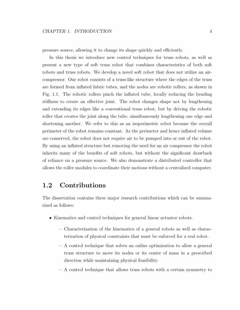
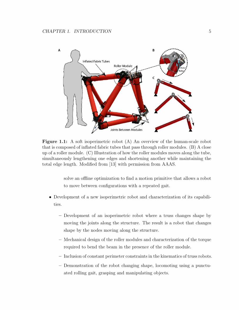
pressure source, allowing it to change its shape quickly and efficiently.
In this thesis we introduce new control techniques for truss robots, as well as
present a new type of soft truss robot that combines characteristics of both soft
robots and truss robots. We develop a novel soft robot that does not utilize an air-
compressor. Our robot consists of a truss-like structure where the edges of the truss
are formed from inflated fabric tubes, and the nodes are robotic rollers, as shown in
Fig. 1.1. The robotic rollers pinch the inflated tube, locally reducing the bending
stiffness to create an effective joint. The robot changes shape not by lengthening
and extending its edges like a conventional truss robot, but by driving the robotic
roller that creates the joint along the tube, simultaneously lengthening one edge and
shortening another. We refer to this as an isoperimetric robot because the overall
perimeter of the robot remains constant. As the perimeter and hence inflated volume
are conserved, the robot does not require air to be pumped into or out of the robot.
By using an inflated structure but removing the need for an air compressor the robot
inherits many of the benefits of soft robots, but without the significant drawback
of reliance on a pressure source. We also demonstrate a distributed controller that
allows the roller modules to coordinate their motions without a centralized computer.
1.2 Contributions
The dissertation contains three major research contributions which can be summa-
rized as follows:
• Kinematics and control techniques for general linear actuator robots.
– Characterization of the kinematics of a general robots as well as charac-
terization of physical constraints that must be enforced for a real robot.
– A control technique that solves an online optimization to allow a general
truss structure to move its nodes or its center of mass in a prescribed
direction while maintaining physical feasibility.
– A control technique that allows truss robots with a certain symmetry to
CHAPTER 1. INTRODUCTION 5
Figure 1.1: A soft isoperimetric robot (A) An overview of the human-scale robotthat is composed of inflated fabric tubes that pass through roller modules. (B) A closeup of a roller module. (C) Illustration of how the roller modules moves along the tube,simultaneously lengthening one edges and shortening another while maintaining thetotal edge length. Modified from [13] with permission from AAAS.
solve an offline optimization to find a motion primitive that allows a robot
to move between configurations with a repeated gait.
• Development of a new isoperimetric robot and characterization of its capabili-
ties.
– Development of an isoperimetric robot where a truss changes shape by
moving the joints along the structure. The result is a robot that changes
shape by the nodes moving along the structure.
– Mechanical design of the roller modules and characterization of the torque
required to bend the beam in the presence of the roller module.
– Inclusion of constant perimeter constraints in the kinematics of truss robots.
– Demonstration of the robot changing shape, locomoting using a punctu-
ated rolling gait, grasping and manipulating objects.
CHAPTER 1. INTRODUCTION 6
– Demonstration of the same set of roller modules being used to create three
different robots.
• A distributed controller for linear actuator robots that allows each node to
communicate with its neighboring nodes to determine local actions that enable
the desired global motion.
– An algorithm, based on consensus alternating direction method of mul-
tipliers (ADMM), that allows each node to reconstruct the shape of the
overall robot using only local communication and measurements
– An algorithm that enables all the nodes to coordinate their actions to
achieve desired motions, even if the desired motions are only known to a
subset of nodes.
1.3 Related Work
In this section we review the relevant literature by first discussing work on truss
robots, and then introducing work on soft robots, and work on enabling truss robots
to act as modular robotic systems.
1.3.1 Truss Robots
Conventional robotic manipulators are typically divided into two classes based on
their kinematic structure: serial and parallel robots. A serial robot consists of a se-
rial chain of actuated revolute or prismatic joints. These robots typically have a large
workspace, but the single path of loading means that they have a relatively low force
output. In a parallel robot, there is more than one loading path to the ground which
offers greater load-bearing capability, but these robots typically have more limited
workspaces than their serial counterparts [14]. The most common architecture of
parallel robots is active struts connected at passive joints to form a truss structure,
thereby leading us to call this family of robots truss robots. The most well-known
parallel robot is the Stewart Platform, which consists of two triangle plates connected
CHAPTER 1. INTRODUCTION 7
with linear actuators at the vertices to form an octahedron structure with 6 active
edges [15]. The Stewart Platform has inspired other types of truss robots with actua-
tors arranged in different truss structures. In this section we will present an overview
of different implementations and applications of truss robots, and leave a detailed
discussion of various control techniques applied to these robots in Chapter 2.
Robots composed of a set of linear actuators arranged in a truss-like architec-
ture were first proposed as variable geometry trusses [16, 17, 18], and were primarily
proposed as lightweight, highly redundant manipulators [19]. Work on TETROBOTs
(Fig. 1.2A) proposed a modular robotic system composed of linear actuators arranged
in repeated graphical motifs of tetrahedrons or octahedrons to facilitate kinematic
computations [20, 21, 22]. These robots have also been proposed as a concept for
planetary landers, as robots with the ability to change shape to adapt to tasks that
may be unknown a priori, or allow locomotion over various terrains (Fig. 1.2B) [1].
Other physical variants of shape-changing robots based on linear actuators include
the modular linear actuator system presented in [23], an octahedron designed for bur-
rowing tasks made of high-extension actuators presented in [24], and an active-surface
type device that uses prismatic joints to deform a surface into arbitrary shapes while
respecting some constraints [25]. In [26], a user interface is presented that allows a
novice user to create a large scale truss structure, and then animate its motion by
inserting a few linear actuators. In [27], a 2D structure is built from a collection of
triangles with linear actuators as their edges, allowing the overall structure to change
shape. Some recent work has focused on a linear actuator robot where the edges
can also actively reconfigure their connectivity as well as their lengths, which have
been called Variable Topology Trusses (Fig. 1.2C) [2,5]. Other work has also focused
specifically on the mechanical design of linear actuator robotic structures [28, 29].
Recent work has produced compact linear actuators that can extend up to ten times
their nominal length [30, 31], making large-scale truss robots with significant shape-
changing capabilities technologically feasible.

CHAPTER 1. INTRODUCTION 8
A B
C D
Figure 1.2: Different implementations of truss type robots and a tensegrity robot.(A) TETROBOT system (B) NASA Ants Project, a tetrahedron composed of highextension linear actuators. (C) Variable Topology Truss (D) The SuperBALL Tenseg-rity robot system. Images from [4] c© 1996 IEEE, [1] c© 2007 IEEE, [5] c© 2017 IEEE,and [32] c© 2017.
Tensegrity Robots
Another class of robots related to but distinct from truss robots are Tensegrity robots,
which consist of a network of rigid bars suspended within a network of compliant ca-
bles (Fig. 1.2D). These robots overcome the brittleness of truss robots by including
inherent compliance through the cables. Tensegrity robots can undergo large shape
changes, especially volume changes for deployment. However, the fact that typically
only a subset of edges change length, and some edges may only support tensile loads,
imposes some constraints on the possible shape change. Tensegrity robots have been
proposed for applications such as space exploration [33, 34], and navigating through
ducts [35]. The robots discussed in this thesis are not tensegrity robots, but our devel-
opment of a soft truss robot was motivated in part by the importance of compliance
CHAPTER 1. INTRODUCTION 9
in truss structures that has been demonstrated by tensegrity robots.
1.3.2 Soft Robots
Soft robots offer the advantage of robustness, inherent safety around human users,
and high tolerance to uncertainty in the environment [3, 7, 36, 37]. These robots
are typically composed of compliant materials and can either stretch or bend to
deform, as opposed to moving about fixed joints. These deformations can be caused
by motor driven tendons, shape memory alloys, or other types of actuation, but
the most prevalent form of actuation is through applying pneumatic or hydraulic
pressure within a cavity. Actuation using pneumatic sources allows large changes
in robot volume, but it creates the fundamental limitation that an air supply is
required. Previous methods to provide pneumatic power on board include carrying
a microcompressor [38, 39], carrying a pressurized fluid reservoir [40], using chemical
decomposition [41], and using explosive fuels [10,42]. However, each of these is limited:
microcompressors have low flow rates and peak pressures, compressed air in a reservoir
has limited overall capacity, and chemical decomposition or burning of a fuel often
requires system-level integration and does not easily provide air at useful pressures
and rates [12]. This thesis presents a new robot design that is composed of an inflated
structure that is maintained at a constant volume, removing the need to carry an air
supply, but maintaining many of the benefits of soft systems.
1.3.3 Collective Robotics
Another advantage of a truss architecture for a robot is its inherent mechanical mod-
ularity. The nodes and edges across a system are often identical, and can be re-
arranged to create new robots. The resulting truss robot behaves as a collective,
with each individual actuator acting as a individual that coordinates its motion with
other actuators to enable motion of the overall robot. Modular robotic systems are
reviewed in [43,44], and in [44] truss-like systems are identified as a subclass of mod-
ular robots. The authors in [29] propose a heterogeneous truss system that can be
CHAPTER 1. INTRODUCTION 10
manually reconfigured, where different links provide power, computation, or actua-
tion, and can be connected at modular nodes. In [23] systems of linear actuators
are used to create several bio-inspired morphing modules. Work on variable topology
trusses have explored truss robots that can autonomously change the connections
between the modules. Leveraging the physical modularity of these systems requires
the development of a modular control architecture as well. Particularly promising is
a distributed control architecture, where instead of requiring a centralized controller
to coordinate motions, individual actuators and joints can determine which actions
to apply locally to produce overall desired behaviors. The TETROBOT is a mechani-
cally modular system, and an accompanying modular and distributed control scheme
was developed where the chain-like architecture of the robot was used to propagate
kinematic and dynamic information between neighbors. Control of a truss robot also
has connections to distance based formation control, which is a well-studied problem
in multirobot systems [45]. In this thesis we present a distributed algorithm that only
requires individual components of the truss robot to communicate with their physical
neighbors, but enables this local coordination to lead to the desired overall behavior
of the robot.
1.4 Dissertation Overview
This dissertation consists of five chapters. This introductory chapter introduces truss,
soft, and collective robots and provided a survey of the relevant literature. Chapter
2 discusses the kinematics of general truss robots, and presents control techniques
to enable a robot to locomote. Chapter 3 introduces a novel isoperimetric soft truss
robot, details its mechanical design, and demonstrates its capabilities. Chapter 3 was
completed in close collaboration with Zachary Hammond, and who was co-first author
for the paper on which the chapter is based [13]. Chapter 4 presents a distributed
estimation and control scheme applied to truss robots. Chapter 5 summarizes the
research, reviews the contributions of the dissertation, and provides possibilities for
future work.

Chapter 2
Locomotion of Truss Robots
Through Kinematic Planning and
Nonlinear Optimization
2.1 Introduction
The ability of a truss-like robot to control many degrees of freedom to change shape
enables it to adapt to different environments and tasks. However, coordinating the
many degrees of freedom to achieve a useful outcome is a challenging control problem
due to the large space of actions that can be applied to the robot. In this chapter,
we present a nonlinear optimization technique to enable a linear actuator robot to
locomote. We present a differential kinematic analysis of truss robots, relating the
velocities of the nodes in the structure to the rate of change of the actuator lengths.
This allows us to link concepts from graph rigidity to the control of the robot struc-
ture. We use this kinematic analysis to derive two on-line planning algorithms for
locomotion which are both based on the same underlying nonlinear optimization algo-
rithm tailored to the kinematics and constraints of a truss robot. A passive mock-up
of a truss robot executing one of the optimized locomotion trajectories presented in
this chapter is shown in Fig. 2.1. In this case, the robot is composed of 10 actuators
(passive car antenna elements), and 5 nodes (with spherical joints formed by magnets
11

CHAPTER 2. KINEMATIC PLANNING FOR TRUSS ROBOTS 12
A B C
D E F
Figure 2.1: We present two algorithms that enable truss robots to locomote. Thisfigure shows snapshots of an optimized everting gait for a truss robot with 10 edgesand 5 vertices, computed with one of our algorithms. The truss robot shown is apassive mockup made from 10 car antennas, and hand-positioned to illustrate thegait. From [46]. c© 2020 IEEE
attached to steel balls).
2.2 Control and Planning Approaches
A variety of different control strategies have been used for past implementations of
truss and tensegrity robots. These methods differ in their use of a model, treatment
of constraints, and whether or not they consider dynamic effects or assume that the
motion of the robot leads to only quasistatic motions. The key challenge is that the
large number of independent actuators create a high-dimensional input space that
can be challenging to explore. Existing work on controlling TETROBOTs focuses
on algorithms for propagating kinematic chains of tetrahedrons or octahedrons [20].
When the motion of certain nodes are specified, [21,22] provide centralized and decen-
tralized algorithms for finding dynamically consistent motions for systems with the
requisite chain architecture. In [47,48] hand designed gaits are presented for use on a
CHAPTER 2. KINEMATIC PLANNING FOR TRUSS ROBOTS 13
particular tetrahedral robot. These gaits are presented as quasistatic paths (trajec-
tories of how the edge lengths change with time, with no accounting for the requisite
forces), and they discuss how the target edge lengths would be used as inputs to a
proportional-integral-derivative (PID) controller that would realize these quasistatic
gaits. The authors in [49] present a dynamic model for a tetrahedral robot, but states
that the dynamics are too complicated for a model based controller, so they use the
kinematic gait presented in [48], but use the dynamics model to better track the tra-
jectory. In [24] the authors also specify motion of an octahedral robot in terms of
kinematic motion of the nodes, and in simulation tests a large family of possible de-
formations. In [50] a rapidly-exploring random tree (RRT) algorithm is used to plan
for a kinematic model of the robot by planning directly in the space of node positions.
This method is generally applicable to arbitrary graph structures, but the large po-
tential space of motions makes it computationally challenging to find a solution, and
heuristics must be used to bias the sampling during the RRT algorithm. These past
results highlight that there is still a need for kinematic planners capable finding gaits
for robots with arbitrary structures in a computationally efficient manner.
Control of tensegrity robots has also received substantial work. Some approaches
use geometric form finding in conjunction with Monte Carlo simulations to determine
useful shapes [51, 52]. If desired trajectories for the node positions are known, the
force density method provides the control inputs to move the equilibrium state of the
robot along a certain path, neglecting dynamics effects [35, 53]. Under a quasistatic
assumption, sampling based planning has been used to find a feasible, but not optimal,
path that avoids collisions [54]. Due to the large state space and input space for the
dynamic system, randomized kinodynamic planning presents a potential approach
[55]. In [56] a sampling based planning technique is used in conjunction with a
dynamic tensegrity simulator, which requires parallelization to be able to operate in
a reasonable timescale. In [57] full kinodynamic planning is used, but in order to make
the problem tractable the authors first introduce an approximate quasi static solution
and use that as a starting point for the kinodynamic sampling. A common approach in
tensegrity robotics is to consider the dynamics but to do so with a learning or adaptive
based approach, including evolutionary style algorithms [52,58, 59], or reinforcement

CHAPTER 2. KINEMATIC PLANNING FOR TRUSS ROBOTS 14
learning [32,60]. The gaits and motions resulting from these approaches leverage the
dynamics, but tend to not fully utilize available information on the known models of
these systems, and it is challenging to adapt these methods to a specific, prescribed
task (moving the center of mass along a trajectory). Other approaches reduce the
problem to a small number of parameters for periodic trajectories [61,62] using central
pattern generators and bayesian optimization. In [63] a dynamic model is used for
offline model predictive control simulations that provide a training set for a deep
learning system. In [64] guided policy search and a reduction of the search space
due to the symmetry of the SUPERball tensegrity robot is used to enable tensegrity
locomotion over non-smooth surfaces. Also leveraging symmetry, [65] proposes a
method to extend a single motion primitive into longer trajectories. A variety of
control approaches to tensegrity robots are reviewed in [66].
We note that while many of the tensegrity control approaches do leverage the
dynamics of the tensegrity system, they do not directly consider a full model based
approach of the dynamics, either treating the dynamics through a data-driven ap-
proach, or employing a method to reduce computation (leveraging symmetry, or using
a kinematic solution as a guide). For this reason, we propose that better quasistatic
planning methods are valuable steps towards improved system performance. We also
note that whereas the dynamics of tensegrity systems often play a large roll in their
response, the linear actuators used in linear actuator robots are often relatively slow,
leading to less emphasis on leveraging the dynamics. In this work we follow the
precedent of the prior work on linear actuator robots and utilize a kinematic model.
2.3 Contributions
In this chapter we present the kinematics of linear actuator robots with arbitrary
graphical structure, including overconstrained structures, and utilize an optimization-
based approach for planning directly over the position of the nodes of the robot. This
optimization approach allows our method to be customized to different tasks and cost
functions. We consider actuator constraints (to enforce min-max elongation), phys-
ical constraints (to prevent self-intersection and enforce a minimum angle between

CHAPTER 2. KINEMATIC PLANNING FOR TRUSS ROBOTS 15
connected actuators), and constraints to avoid kinematic singularities in arbitrary
robots in designing locomotion algorithms. The key contributions of this work are
two algorithms to solve the following problem:
Problem 1 Move the center of mass of the robot in a prescribed direction vcm, or
along a prescribed trajectory xcm(τ), ensuring that the robot is always physically fea-
sible and that the robot does not pass through any singular configurations.
The first algorithm we propose solves an online optimization to minimize an ob-
jective function that considers only the current state and motion of the robot while
ensuring physical feasibility. This method applies to any robot that is in an infinites-
imally rigid configuration. However, this method does not guarantee the persistent
feasibility of the robot’s motion, meaning it is possible the robot will reach a config-
uration from which it cannot continue without violating physical constraints (i.e., it
might get tangled up). To ensure persistent feasibility, we present another method
where we solve an offline optimization that generates periodic motion primitives to
move a robot from a starting configuration to an equivalent configuration centered on
a new support polygon. This motion primitive is then used by a high-level planner
to plan paths from an initial configuration to a goal. We refer to this method as
the two-tiered planning approach. This method guarantees persistent feasibility of
the trajectory, but requires that the initial configuration of the robot satisfy certain
symmetry requirements. The performance of the two algorithms is compared in sim-
ulation study in which we find that the two-tiered planning approach gives better
performance in terms of cost.
Portions of this chapter have been previously published in [46, 67]. We also note
that the work presented in the conference paper [67] has served as the foundation of
the work in [50,68].
The rest of the chapter is organized as follows: Sec. 2.4 formalizes a model for
LARs and derives the forward and inverse kinematics relating the change in actuator
lengths to node positions. Sec. 2.5 describes the physical constraints imposed to
ensure the robot motion is feasible. Our single step locomotion algorithm is given
in Sec. 2.6, and our two-tiered approach is presented in Sec. 2.7. These methods are
CHAPTER 2. KINEMATIC PLANNING FOR TRUSS ROBOTS 16
compared in Sec. 2.8. In Sec. 2.9 we discuss the performance of the kinematic plan
in the presence of dynamic effects, and conclusions are given in Sec. 2.10.
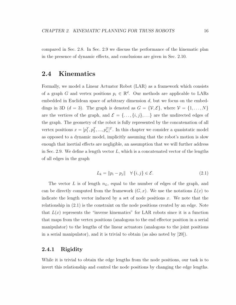
2.4 Kinematics
Formally, we model a Linear Actuator Robot (LAR) as a framework which consists
of a graph G and vertex positions pi ∈ Rd. Our methods are applicable to LARs
embedded in Euclidean space of arbitrary dimension d, but we focus on the embed-
dings in 3D (d = 3). The graph is denoted as G = {V , E}, where V = {1, . . . , N}are the vertices of the graph, and E = {. . . , {i, j}, . . .} are the undirected edges of
the graph. The geometry of the robot is fully represented by the concatenation of all
vertex positions x = [pT1 , pT2 , ..., p
Tn ]T . In this chapter we consider a quasistatic model
as opposed to a dynamic model, implicitly assuming that the robot’s motion is slow
enough that inertial effects are negligible, an assumption that we will further address
in Sec. 2.9. We define a length vector L, which is a concatenated vector of the lengths
of all edges in the graph
Lk = ‖pi − pj‖ ∀ {i, j} ∈ E . (2.1)
The vector L is of length nL, equal to the number of edges of the graph, and
can be directly computed from the framework (G, x). We use the notations L(x) to
indicate the length vector induced by a set of node positions x. We note that the
relationship in (2.1) is the constraint on the node positions created by an edge. Note
that L(x) represents the “inverse kinematics” for LAR robots since it is a function
that maps from the vertex positions (analogous to the end effector position in a serial
manipulator) to the lengths of the linear actuators (analogous to the joint positions
in a serial manipulator), and it is trivial to obtain (as also noted by [20]).
2.4.1 Rigidity
While it is trivial to obtain the edge lengths from the node positions, our task is to
invert this relationship and control the node positions by changing the edge lengths.
CHAPTER 2. KINEMATIC PLANNING FOR TRUSS ROBOTS 17
In a network of linear actuators, each link length imposes one constraint on the node
positions as given in (2.1). Finding the vertex positions from the link lengths means
finding node positions that satisfy all of the constraint equations up to translation and
rotation of the entire network. Several classes of solutions exist based on the rigidity
of the underlying graph. Examples of a few of these classes are shown in Fig. 2.2,
and our analysis of the device kinematics in the following section will depend on the
rigidity of the underlying graph of the robot. If the system of equations has infinite
solutions the framework is not rigid, as it is possible to move the system relative to
itself without violating length constraints as in Fig. 2.2(i). A framework is rigid if
there are a discrete number of solutions to the constraint equations, and all deflections
of the system relative to itself violate the length constraints.
Of particular use to our analysis are graphs that are infinitesimally rigid, meaning
that all infinitesimal deflections of the system relative to itself violate the length
constraints. Infinitesimal rigidity is dependent on the configuration x and is not an
inherent characteristic of the graph G. Infinitesimally rigid frameworks are a subset of
rigid frameworks, meaning a framework can be rigid but not infinitesimally rigid, but
all infinitesimally rigid frameworks are also rigid. Fig. 2.2(ii) shows an infinitesimally
rigid framework, while the one in Fig. 2.2(iii) is rigid but not infinitesimally rigid.
Of particular interest in the design of LARs are minimally rigid graphs. A mini-
mally rigid graph is a rigid graph where the removal of any link causes the graph to
lose rigidity. These minimally rigid graphs provide a lower bound on the number of
links necessary to constrain a certain number of nodes. For a graph in 3 dimensions,
at least 3n− 6 edges are necessary for minimal rigidity, which can be understood in-
tuitively based on a degree of freedom argument. Each node in R3 has three degrees
of freedom, and each edge imposes a constraint that removes at most one degree of
freedom. The final structure has 6 degrees of freedom in its rigid body motion (3
translational, and 3 rotational). An infinitesimally rigid graph in R3 with 3n − 6
edges is minimally rigid, although 3n − 6 edges does not necessarily imply rigidity.
In Fig. 2.2 the framework in (ii) is infinitesimally minimally rigid, framework (iii)
is minimally rigid but not infinitesimally rigid, and framework (iv) is infinitesimally
rigid and over-constrained.
CHAPTER 2. KINEMATIC PLANNING FOR TRUSS ROBOTS 18
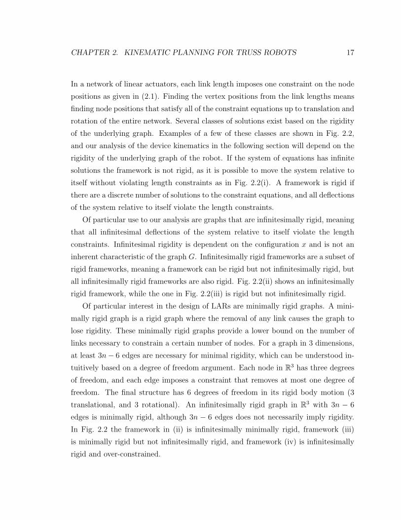
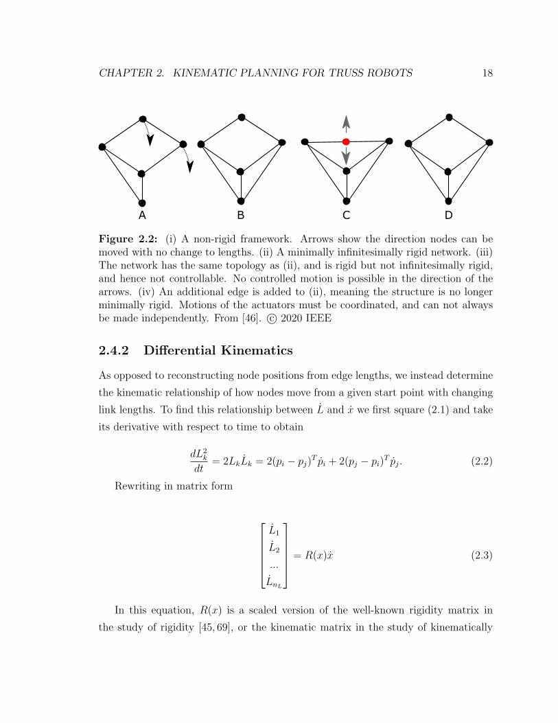
A B C D
Figure 2.2: (i) A non-rigid framework. Arrows show the direction nodes can bemoved with no change to lengths. (ii) A minimally infinitesimally rigid network. (iii)The network has the same topology as (ii), and is rigid but not infinitesimally rigid,and hence not controllable. No controlled motion is possible in the direction of thearrows. (iv) An additional edge is added to (ii), meaning the structure is no longerminimally rigid. Motions of the actuators must be coordinated, and can not alwaysbe made independently. From [46]. c© 2020 IEEE
2.4.2 Differential Kinematics
As opposed to reconstructing node positions from edge lengths, we instead determine
the kinematic relationship of how nodes move from a given start point with changing
link lengths. To find this relationship between L and x we first square (2.1) and take
its derivative with respect to time to obtain
dL2k
dt= 2LkLk = 2(pi − pj)T pi + 2(pj − pi)T pj. (2.2)
Rewriting in matrix form
L1
L2
...
LnL
= R(x)x (2.3)
In this equation, R(x) is a scaled version of the well-known rigidity matrix in
the study of rigidity [45, 69], or the kinematic matrix in the study of kinematically

CHAPTER 2. KINEMATIC PLANNING FOR TRUSS ROBOTS 19
indeterminate frameworks [70]. Each row of R(x) represents a link Lk. For example,
let row k represent the link between nodes i and j. The only non-zero values of row
k are R(x)k,(3i−2,3i−1,3i) =(pi−pj)‖Lk‖
, and R(x)k,(3j−2,3j−1,3j) =(pj−pi)‖Lk‖
. Note that in the
standard rigidity matrix the entries are of the form (pj − pi) and not(pj−pi)‖Lk‖
, hence
we refer to R(x) as the scaled rigidity matrix. For a graph with n vertices, NL edges,
and the positions of the vertices given in Rd, then R ∈ RNL,nd. For d = 3, the
maximum rank of R is 3n−6. If the matrix R(x) is of maximum rank, the framework
is infinitesimally rigid [69].
2.4.3 Contact with the Ground
In addition to the relationship between actuator lengths and vertex positions, we
must capture the robot’s interaction with the environment. Sufficient constraints
between the robot and the environment must be used to ensure that the location of
the structure is fully defined (6 independent relationships when the structure is in R3).
For this work we assume that three of the robot’s nodes on the ground form a support
polygon, and that the nodes that make up the support polygon do not slide across the
ground. If after applying some control the center of mass leaves the support polygon,
the structure rolls about the edge of the support polygon closest to the center of mass
until the next point comes into contact with the ground. This process is repeated
until the center of mass is inside the support polygon. This assumption is valid for
many cases, but it does neglect the dynamic nature of the rolling transition. The
decision that the support feet do not move along the ground is restrictive, but means
that the gaits are somewhat robust to changes in the ground properties, and do not
depend on friction models of the ground.
We encode these relationships in terms of the equation Cx = 0 where each row of
C has one nonzero entry that is equal to 1, such that each row of C makes one node
of the robot stationary in one coordinate of the environment. For a minimal set of
constraints, C ∈ R6, 3n. We choose this minimum set of constraints such that one of
the support feet is fixed in all three dimensions, another support foot is fixed in the
vertical direction and one of the lateral directions, and the last support foot is fixed
CHAPTER 2. KINEMATIC PLANNING FOR TRUSS ROBOTS 20
only in the vertical direction. If we constrain the 3 nodes of the support polygon to
be unable to move, C ∈ R9, 3n. In the future we could expand the contact constraints
to the form Cx = F where F represents some motion of the environment and the
C matrix potentially captures a different type of interaction with the environment.
For example, this framework could enforce an interaction where the robot’s feet could
slide on the ground or be supported against moving obstacles.
2.4.4 Kinematic Model
We combine the kinematic model with the contact model to obtain the following
differential kinematics:
[L
0
]=
[R(x)
C
] [x]
= H(x)x. (2.4)
If the system is infinitesimally minimally rigid and a minimal set of constraints
is applied that is linearly independent of the link constraints, the combined matrix
H = [RT CT ]T is full rank and square, and hence invertible, allowing us to write
x = H(x)−1
[L
0
]. (2.5)
Note that this is the form of a driftless dynamical system, and that H(x)−1 is
the Jacobian matrix relating the motion of the actuators to the motion of the nodes.
The vector L describes the rates of change of the linear actuators, and hence is the
input to the system. Equation (2.5) shows that when the H(x) is invertible, each
input channel Lk can be commanded independently of the others. The fact that
this matrix is invertible means that the input space is all possible length velocities,
allowing us to make the following proposition:
Proposition 1 Given an infinitesimally minimally rigid framework with the mini-
mum number of constraints to the environment, the length of each edge can change
CHAPTER 2. KINEMATIC PLANNING FOR TRUSS ROBOTS 21
independently.
This means that it is not necessary to coordinate movements between lengths as
long as the graph remains minimally infinitesimally rigid.
2.4.5 Controlling Over-Constrained Networks
If the system is infinitesimally rigid but not minimally rigid, it is over-constrained and
some motions of the linear actuators must be coordinated. In this case, the H matrix
is skinny, with more rows than columns. Taking the singular value decomposition of
the combined H matrix,
UT
[L
0
]= ΣV T x, (2.6)
[UT1
UT2
][L
0
]=
[Σ
0
]V T x. (2.7)
The bottom rows of this expression can be expressed as a constraint which encod-
ing how certain lengths must move in a coordinated fashion:
UT2
[L
0
]= 0. (2.8)
By utilizing this constraint, redundant rows of the H matrix and their correspond-
ing elements in the vector [LT 0]T can be removed until it is square and full rank,
and hence invertible. We call the reduced H matrix and L vector the master group,
and we denote them as Hm and Lm respectively. We refer to the removed rows as the
slave group, and denote as Hs, and the removed actuator inputs as Ls. We note that
the actuators chosen for the master and slave groups are partially up to the user’s
discretion, and could potentially change based on configuration. As an example pro-
cedure, an algorithm could initialize Hm = H, and Hs as an empty matrix, and then
iterate through each row of the Hm matrix. If it finds a row linearly dependent on the
CHAPTER 2. KINEMATIC PLANNING FOR TRUSS ROBOTS 22
previous rows from the Hm matrix and places it in Hs, and removes the corresponding
element of Lm and places it in Ls. This allows us to express the system as follows:
x =[Hm(x)
]−1 [Lm0
](2.9)
s.t. Ls = Hs(x)Hm(x)−1
[Lm
0
]. (2.10)
Due to (2.10) the input space is restricted such that only combinations of link
velocities that satisfy the constraint can be physically realized. The master inputs
Lm can be picked arbitrarily, but Ls must be chosen to satisfy the constraint equation.
This system can be expressed in the standard form of a linear dynamical system,
x = Ax + Bu where A = 0, u = [LT 0T ]T , and B = Hm(x)−1. We now make the
following proposition:
Proposition 2 A framework that is infinitesimally rigid is fully actuated.
This means that for an infinitesimally rigid system control of every degree of
freedom can be achieved given control of the rate of change of the actuator lengths
and the motion of the contact points. This has the key advantage of allowing us to
plan our motion in terms of node positions, and then use the [RT CT ]T matrix to
determine what input to apply to the actuators.
2.5 Physical Constraints
Locomotion requires finding a method to actuate the robot to move while it maintains
physical feasibility. We define feasibility as follows:
Definition 1 A framework (G, x) is feasible if it meets three types of physical con-
straints: (i) the lengths of all actuators fall within a fixed maximum and minimum
length range, (ii) the actuators do not physically intersect (except at the endpoints of

CHAPTER 2. KINEMATIC PLANNING FOR TRUSS ROBOTS 23
two connected actuators), and (iii) the angles defined by two actuators connected at
a joint remain above a minimum value.
To ensure that all motions of the robot are physically feasible, we detail the form
of the constraints and quantify how many of each type of constraint occurs in the
optimization based on the characteristics of the underlying graph. In addition to these
physical constraints, we also present constraints to prevent the robot from crossing
configurations where infinitesimally rigidity is lost, which correspond to the singular
configurations of the robot.
2.5.1 Length Constraints
For physical feasibility to be preserved, all actuators must be maintained between
a maximum and minimum actuator length. The squared length of actuator k that
connects nodes {i, j} is quadratic in x, and the constraint that it remain within the
set maximum and minimum length can be expressed as
L2min ≤ xT
[Id ⊗ Ak
]x ≤ L2
max. (2.11)
where Ak is a matrix where the only nonzero entries are Ak,ii = Ak,jj = 1, Ak,ij =
Ak,ji = −1. We note that constraints of the quadratic form xTQx ≤ c, where c is a
positive constant, are convex if and only if Q is positive semi-definite. We note that
Ak is the Laplacian matrix of a graph that contains only edge k. As the Laplacian
matrix is always positive semi-definite, the maximum length constraint is convex in
the node positions while the minimum length constraint is not. Thus our algorithms
will handle non-convex and nonlinear constraints.
2.5.2 Distance Between Actuator Constraints
We also enforce the constraint that actuators do not collide physically, except for at
the vertices where they are joined. To determine if two actuators cross, the mini-
mum distance between them must be greater than dmin, a positive diameter of the
actuator assuming that the actuator can be represented as a cylinder. The minimum
CHAPTER 2. KINEMATIC PLANNING FOR TRUSS ROBOTS 24
distance between actuators connecting vertices i, j and k, l is denoted as dklij , and can
be expressed as follows:
dklij = min‖(pi + α(pj − pi))− (pk + γ(pl − pk))‖ α, γ ∈ (0, 1) (2.12)
These links are not in collision if dklij > dmin. Efficient algorithms for this computation
have been explored previously [71]. Checking the pairwise distances between all edges
in a graph requires checkingN2
L−NL
2constraints of the type expressed in (2.12). As
we do not compute the distance between actuators that are connected at a node, the
number of constraints is reduced by the number of pairwise distances between edges
that meet at a node, which for node i is given byg2i−gi
2where gi is the degree of the
node. Thus the total number of constraints to avoid collisions between actuators is
N2L −NL
2−
n∑i=1
g2i − gi2
. (2.13)
2.5.3 Angle Constraints
Another key physical constraint is that the angle between connected actuators remain
above a certain value, which is especially important when the actuators have a high
elongation ratio. An angle constraint between two edges is a function of 3 vertices.
We define pi as the position of the shared node between two edges, and pj and pk as
the other vertices of the two edges. The angle constraint is:
cos(θmin) ≤ (pj − pi)T (pk − pi)‖pj − pi‖‖pk − pi‖
(2.14)
The number of angle constraints can also be expressed in terms of the degree of
the nodes of the graph:
−NL +1
2
n∑i=1
g2i . (2.15)

CHAPTER 2. KINEMATIC PLANNING FOR TRUSS ROBOTS 25
2.5.4 Rigidity Maintenance Constraint
Our proposed optimization approach is based on the observation that if the robot
is infinitesimally rigid, we can directly optimize a path for the node positions and
recreate the needed actuator trajectories. For this assumption to remain valid, the
robot must maintain its infinitesimal rigidity, meaning the rigidity matrix R must
remain of rank 3n− 6. Designing controllers that maintain infinitesimal rigidity has
been a topic in formation control of multi-agent systems [72, 73]. In [72] the rigidity
eigenvalue for frameworks in R3 is defined as the 7th smallest eigenvalue of R(x)TR(x)
and the gradient of the rigidity eigenvalue with respect to the node positions is used
as part of a controller. In the general case, infinitesimal rigidity can be enforced using
the following constraint:
λ7 > λcrit (2.16)
where λ7 is the 7th smallest eigenvalue of the R(x)TR(x) matrix and λcrit is its
minimum allowable value.
One problem with (2.16) is that the magnitude of λ7 changes quadratically with
network size. To provide a constraint that is invariant to network scale, we instead
use the worst case rigidity metric, taken directly from [74], and defined as:
λ7∑3ni=1 λi
=λ7
tr(R(x)TR(x))=
λ7∑NL
i=1(L(x)i)2≥ λcrit (2.17)
It has been noted that if a framework is infinitesimally rigid in one configuration
it is infinitesimally rigid almost everywhere, meaning that for a graph with one in-
finitesimally rigid configuration, the set of non-rigid configurations is a set of zero
measure [75]. We make the observation that the configurations where the robot loses
rigidity often divide the state space into disconnected regions. We define each of these
regions as a rigidity equivalence class as follows:
Definition 2 (Rigidity Equivalence Class) The framework F1 = (G,X1) and the
framework F2 = (G,X2) are in the same rigidity equivalence class if a continuous
path x(t) exists such that x(0) = X1, x(T ) = X2, and the rigidity matrix R(G, x(t))
is maximal rank for all t ∈ (0, T ).

CHAPTER 2. KINEMATIC PLANNING FOR TRUSS ROBOTS 26
Figure 2.3: The values of the Worst Case Rigidity index (2.17) as the position ofnode E changes linearly between the left and right configurations. Without edge CE(shown in yellow) the worst case rigidity index goes to 0 when E is co-planar withDAB, while with the yellow edge, the worst case rigidity index remains greater than1. From [46]. c© 2020 IEEE
Analytically characterizing these rigidity equivalence classes for an arbitrary graph
has proved challenging. However, we are able to make a statement for the case of
graphs that contains 3-simplex (a complete tetrahedron) as a subgraph. For each
complete tetrahedron, we define its orientation as the sign of the signed volume which
is computed as
V = (p4 − p1)T (p3 − p1)× (p2 − p1). (2.18)
These preliminaries allow us to make the following statement:

CHAPTER 2. KINEMATIC PLANNING FOR TRUSS ROBOTS 27
Theorem 1 Let F1 = (G,X1) and F2 = (G,X2) be two minimally rigid frameworks
in R3. If there exists a subgraph of G that is a 3-simplex and F1 and F2 contain
the simplex with opposite orientation, the two frameworks lie in different equivalence
classes.
Finding a smooth path x(t) for the vertices of a simplex from one orientation to
the other requires the signed volume to smoothly change signs, passing a configuration
where V = 0. When V = 0 for a simplex, one of the edges of the simplex is a linear
combination of the others, meaning there is a redundant edge in the R matrix. For a
minimally rigid graph the R matrix has 3n− 6 rows, so any linearly-dependent edges
indicate the matrix is not maximal rank and hence not infinitesimally rigid.
One general question in the design of linear actuator robots is if an over-constrained
network is necessary, or if a minimally rigid network is sufficient. We give an exam-
ple where an over-constrained robot can achieve motion through a configuration that
would represent a singularity were the robot minimally rigid (shown in Fig. 2.3).
In this example, we first consider the robot to be only composed of the blue edges
(edge CE is not present). In this case both the left and right configurations are in-
finitesimally rigid and simplex ABED has different orientation in each configuration,
meaning that the two configurations lie in different rigidity equivalence classes by the-
orem 1. If the node positions are linearly interpolated between the two configurations,
the rigidity index in (2.17) goes to 0 when node E is coplanar with nodes ABD. The
addition of the yellow edge, which makes the robot over-constrained, allows rigidity
to be maintained throughout the transition, as shown by the plot in Fig. 2.3. We
note that with the yellow edge this graph is the fully connected 5-node graph, known
as the K5 graph. The K5 graph displays another interesting property:
Theorem 2 The rigidity matrix R(x) for a robot represented by a complete graph of
5 or more nodes only loses rank at configurations where the robot has actuators in
collision.
For a node in a complete graph to have an unconstrained infinitesimal motion, its
neighboring edges must not span R3, meaning that all nodes must lie in the plane.
Complete graphs with 5 or more nodes do not have planar non-crossing embeddings.
CHAPTER 2. KINEMATIC PLANNING FOR TRUSS ROBOTS 28
This result means enforcing the constraint that no actuators collide for the K5
graph naturally enforces the graph rigidity constraint. Whenever we evaluate a K5
robot in this chapter, we leverage this result and do not enforce the rigidity mainte-
nance constraint.
2.5.5 Constraint Satisfaction Between Timesteps
Our approach to finding a trajectory for a linear actuator robot is to use an optimiza-
tion to solve for a discretized trajectory containing Nconfig configurations we denote
as xj where j = 1, 2, ...Nconfig. The optimization solution guarantees that the config-
urations xj satisfy the constraints defined above which we now succinctly express as
f(xj) ≤ 0. However, the nonconvex nature of the constraints means that it is possible
that the intermediate configurations (the configurations between xj and xj+1) may
violate the constraints. To address this, we enforce a constraint that two sequential
configurations must be close together in terms of the distance each node travels. We
define this constraint as
‖pji − pj−1i ‖ ≤ dmove ∀i. (2.19)
We assume that the intermediate configurations between xji and xj−1i are given
by linear interpolation. From work on sampling-based motion planning [76], the
maximum violation of a constraint between two configurations can be bounded by
using the Lipschitz constant, K of the constraint as follows
∣∣f(xj)− f(xk)∣∣ ≤ K‖xj − xk‖. (2.20)
Given the Lipschitz constant for each constraint function, it is possible to augment
the constraints with a buffer such that satisfying the buffered constraints and the
constraint in 2.19 ensures satisfaction of the true constraint. In our case, we assume
that the constraints already include this buffer. In practice we choose dmove to ensure
that two edges can not jump over each other without violating the collision constraint
by picking 2dmove ≤ dmin.
CHAPTER 2. KINEMATIC PLANNING FOR TRUSS ROBOTS 29
2.6 Single Step Locomotion
Our first approach to solving the locomotion problem involves solving an online op-
timization to move the center of mass to a desired position for one time step. It
acts greedily to minimize an objective function for a time step, and does not account
for making and breaking contact with the ground. Our second method, presented in
Sec. 2.7 and referred to as a two-tiered planning approach, extends this single step
computation to an optimization over multiple steps. The two-tiered approach directly
accounts for the rolling behavior in the computation, but imposes restrictions that
the robot must satisfy certain symmetry requirements.
2.6.1 Controlling the Velocity of the Center of Mass
The position of the center of mass is defined in terms of the mass matrix of the system,
M ∈ R3×3n. Without loss of generality, the quasistatic model allows us to assume
that all mass is concentrated at the nodes of the system. In our case, we assume that
all actuators are of uniform, evenly distributed mass, and thus half of the mass is
assigned to each end of the actuator. The position of the center of mass is given by
xcom = Mx =[mvec ⊗ I3,
]x (2.21)
where mvec,i is the sum of all of the partial masses assigned to node i. In the
uniformly distributed case, mvec,i = di2NL
. With this mass matrix, we can express the
velocity of the center of mass as a function of the actuator velocities
xcom = Mx = MH−1L. (2.22)
We can now pick any L that achieves a desired motion of the center of mass. The
maximum rank of M is d, so for a system with many vertices MH−1 will have more
columns than rows, and there is freedom in which x is selected to move the center
CHAPTER 2. KINEMATIC PLANNING FOR TRUSS ROBOTS 30
of mass. We define an optimization problem to pick a value of L that minimizes an
objective function.
2.6.2 Optimization Setup
The kinematic relationships derived in the Sec. 2.4 apply to a continuous time system.
To optimize the trajectory we work in discrete time, denoting the configuration of the
robot with the superscript xj. In practice we determine the node velocities by linearly
interpolate from the current configuration to the configuration that is the result of
the optimization, and determine the necessary actuator velocities using the kinematic
relationships. The optimization procedure takes as an input the configuration at xj−1
and optimize the next desired configuration xj. We seek to find a trajectory that
maximizes some cost function J(x) while satisfying constraints. As this optimization
minimizes the cost function over only one step, we refer to this optimization approach
as the greedy method. The complete optimization problem is given as follows:
minxj
J(xj) (2.23)
subject to
Cxj = b (2.24)
Gxj ≥ 0 (2.25)
f(xj) ≤ 0 (2.26)
‖xji − xj−1i ‖ ≤ dmove ∀i (2.27)
The choice of cost function J(x) will be discussed in the following section. Eq. (2.24)
fixes the contact points and is the discrete time version of the ground constraint, where
b is a vector of locations of the vertices in the support polygon. In the locomotion
optimization we also enforce the linear constraint that no nodes pass through the
ground, Gx > 0, where G = In ⊗ diag([0 0 1]). We denote all of the feasibility
constraints, including maximum and minimum actuator length (2.11), actuator colli-
sion constraints (2.12), angle constraints (2.14), and singularity avoidance constraints

CHAPTER 2. KINEMATIC PLANNING FOR TRUSS ROBOTS 31
(2.17) as f(xj) ≤ 0 as given in (2.26).
2.6.3 Objective Function
By defining this problem as an optimization problem, the system will take the action
that instantaneously optimizes some objective, J(x). One intuitive choice for the cost
function is J(x) = ‖L(x)‖2 = ‖R(x)x‖2, which penalizes large actuator velocities. In
discrete time, we approximate this cost as:
J(x) = ‖L(xj)− L(xj−1)‖2 (2.28)
As mentioned previously, one potential issue with a single-step method is that
persistent feasibility is not guaranteed. One heuristic to prevent the robot from
getting tangled up in an unfavorable configuration, derived from simulation testing,
is to try and keep the network as close as possible to a fixed operating point, such as
attempting to keep all actuators close to a nominal length lN . This can be encoded
with an objective function
J(x) = ‖L(xj)− lN‖2. (2.29)
We will quantitatively compare the results of using both of these cost functions in
Section VI.
2.6.4 One Step Optimization Results
We find a feasible solution to the optimization problem using the sequential quadratic
programming algorithm available in the matlab fmincon toolbox. The most computa-
tionally expensive part of this algorithm is repeatedly checking to see if the nonlinear
constraints are violated, a process that could be parallelized in a future implemen-
tation. To speed computation, ∂f(x)∂x
is computed analytically before operation. We
demonstrate the character of the solutions that result from this optimization we will
show the types of trajectories generated when it is applied to different robots in the
following sections.
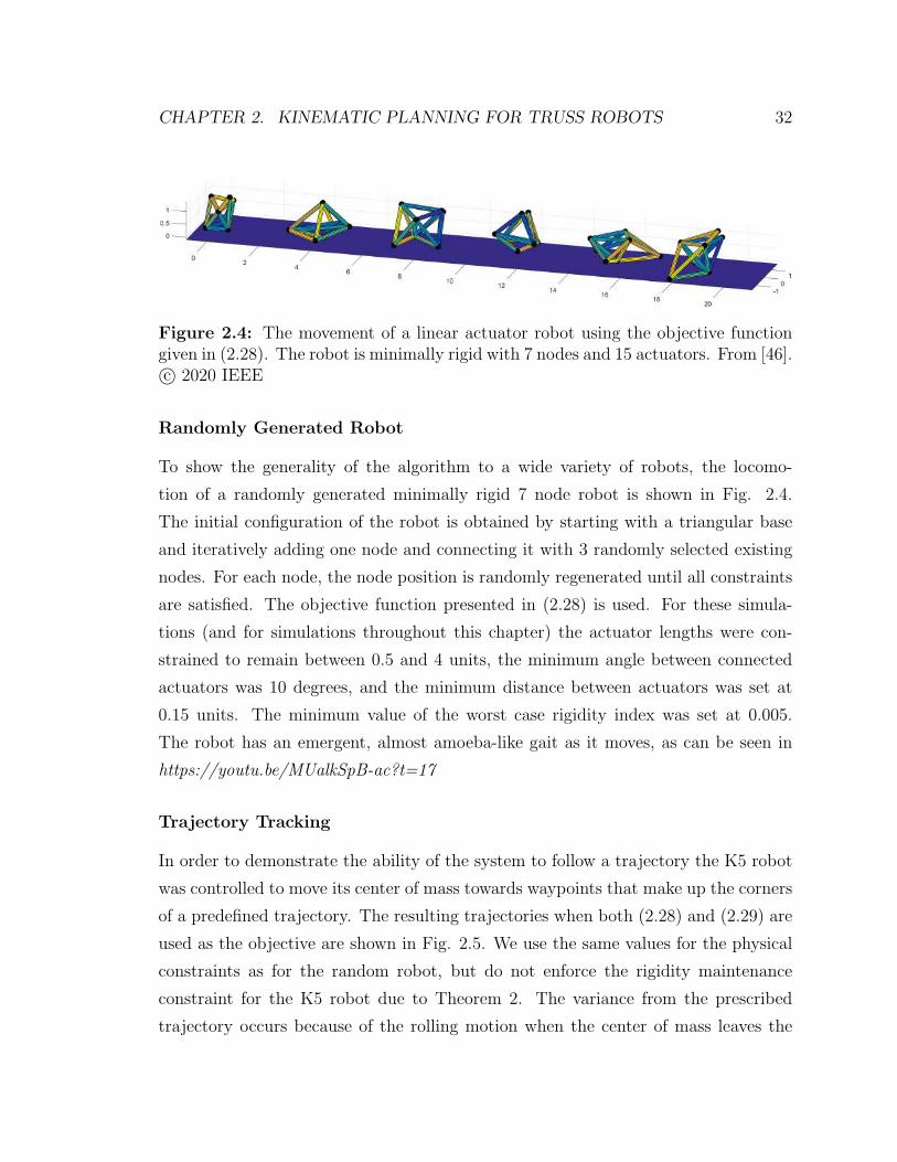
CHAPTER 2. KINEMATIC PLANNING FOR TRUSS ROBOTS 32
Figure 2.4: The movement of a linear actuator robot using the objective functiongiven in (2.28). The robot is minimally rigid with 7 nodes and 15 actuators. From [46].c© 2020 IEEE
Randomly Generated Robot
To show the generality of the algorithm to a wide variety of robots, the locomo-
tion of a randomly generated minimally rigid 7 node robot is shown in Fig. 2.4.
The initial configuration of the robot is obtained by starting with a triangular base
and iteratively adding one node and connecting it with 3 randomly selected existing
nodes. For each node, the node position is randomly regenerated until all constraints
are satisfied. The objective function presented in (2.28) is used. For these simula-
tions (and for simulations throughout this chapter) the actuator lengths were con-
strained to remain between 0.5 and 4 units, the minimum angle between connected
actuators was 10 degrees, and the minimum distance between actuators was set at
0.15 units. The minimum value of the worst case rigidity index was set at 0.005.
The robot has an emergent, almost amoeba-like gait as it moves, as can be seen in
https://youtu.be/MUalkSpB-ac?t=17
Trajectory Tracking
In order to demonstrate the ability of the system to follow a trajectory the K5 robot
was controlled to move its center of mass towards waypoints that make up the corners
of a predefined trajectory. The resulting trajectories when both (2.28) and (2.29) are
used as the objective are shown in Fig. 2.5. We use the same values for the physical
constraints as for the random robot, but do not enforce the rigidity maintenance
constraint for the K5 robot due to Theorem 2. The variance from the prescribed
trajectory occurs because of the rolling motion when the center of mass leaves the

CHAPTER 2. KINEMATIC PLANNING FOR TRUSS ROBOTS 33
support polygon. In order to illustrate the effectiveness of this method in preventing
constraints from being violated, Fig. 2.6 shows that during the trajectories shown in
Fig. 2.5, the various physical constraints on the robot are often active but are not
violated.
This trajectory tracking test also gives a sense of the robustness of the control
algorithm. A downside to the approach of repeatedly solving the optimization is that
persistent feasibility is not guaranteed, meaning it is possible that the network reaches
a configuration where it cannot continue without violating some constraint. In the
case where the objective function was (2.28), a configuration was reached where the
device could not continue to match the desired center of mass motion without violating
constraints (the blue trajectory in Fig. 2.5). With the objective presented in (2.29),
the planner finds a feasible path that completes the trajectory (the red trajectory in
Fig. 2.5). Simulation results on a variety of trajectories show that a common failure
mode of the system is if the robot rolls onto a very large support polygon, it may
not have the ability to extend its center of mass and roll again. This failure mode
may become less significant if future work included a frictional model of the ground
and allowed the support nodes to slide along the ground. Interestingly, relaxing
constraints does not necessarily guarantee the robot will be able to travel further
before reaching a configuration with no feasible solution. Often, relaxed constraints
such as a higher upper limit on actuator length lead to failure sooner, as the robot
tends to reach more jumbled configurations early in the trajectory. Computation for
completing the “S” trajectory involved solving the one-step optimization 1893 times,
which took approximately 120 seconds on a laptop computer (Intel Core i7 Processor,
4 cores, 2.80 GHz, 16GB RAM). The average time to solve each optimization was 63
ms, with a standard deviation of 10 ms and a maximum time of 153 ms.
Note that at each time step these methods instantaneously minimize an objective
while a desired motion of the center of mass is obtained. The algorithm can be
thought of as greedily trying to move the center of mass. However, motion is not
optimal for the entirety of the trajectory. The algorithm does not explicitly take into
account making and breaking of contact with the surface, which would be required
to discuss the optimality of an entire trajectory. To enable discussion of optimality
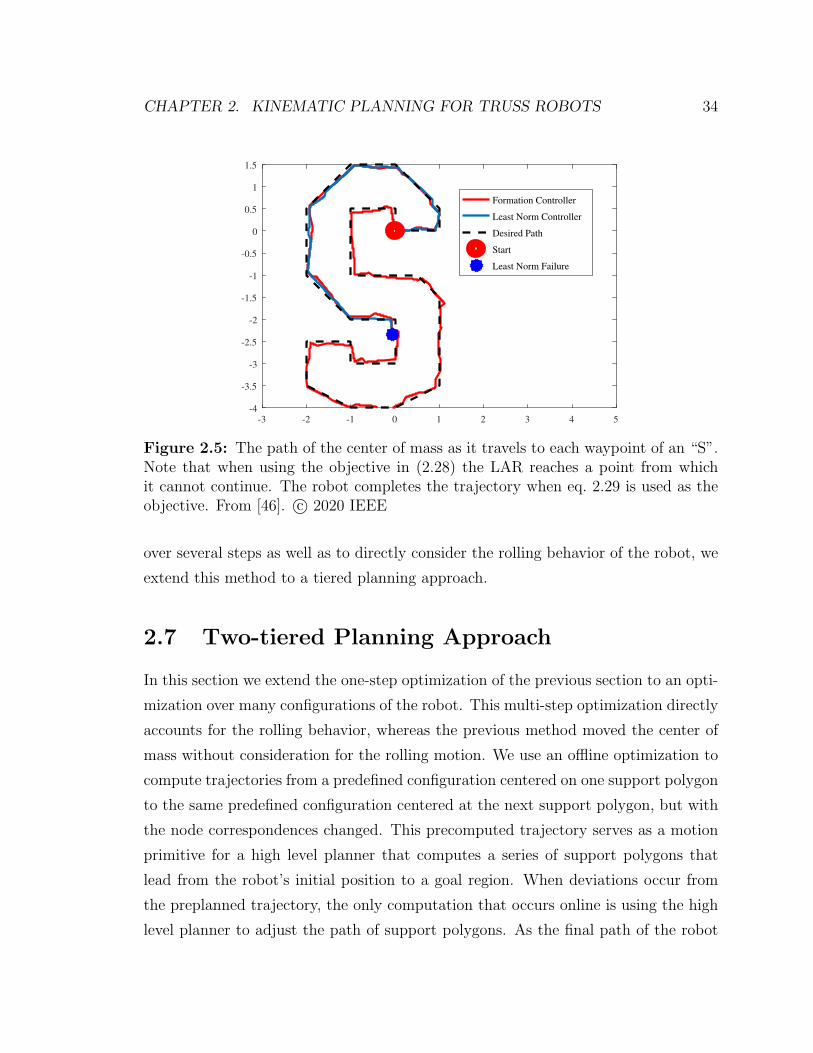
CHAPTER 2. KINEMATIC PLANNING FOR TRUSS ROBOTS 34
-3 -2 -1 0 1 2 3 4 5
-4
-3.5
-3
-2.5
-2
-1.5
-1
-0.5
0
0.5
1
1.5
Formation Controller
Least Norm Controller
Desired Path
Start
Least Norm Failure
Figure 2.5: The path of the center of mass as it travels to each waypoint of an “S”.Note that when using the objective in (2.28) the LAR reaches a point from whichit cannot continue. The robot completes the trajectory when eq. 2.29 is used as theobjective. From [46]. c© 2020 IEEE
over several steps as well as to directly consider the rolling behavior of the robot, we
extend this method to a tiered planning approach.
2.7 Two-tiered Planning Approach
In this section we extend the one-step optimization of the previous section to an opti-
mization over many configurations of the robot. This multi-step optimization directly
accounts for the rolling behavior, whereas the previous method moved the center of
mass without consideration for the rolling motion. We use an offline optimization to
compute trajectories from a predefined configuration centered on one support polygon
to the same predefined configuration centered at the next support polygon, but with
the node correspondences changed. This precomputed trajectory serves as a motion
primitive for a high level planner that computes a series of support polygons that
lead from the robot’s initial position to a goal region. When deviations occur from
the preplanned trajectory, the only computation that occurs online is using the high
level planner to adjust the path of support polygons. As the final path of the robot
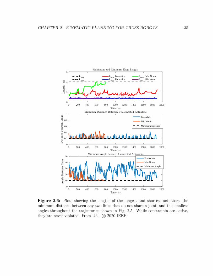
CHAPTER 2. KINEMATIC PLANNING FOR TRUSS ROBOTS 35
0 200 400 600 800 1000 1200 1400 1600 1800 20000
2
4
6
Lmax
Lmin
Lmax
Formation
Lmin
Formation
Lmax
Min Norm
Lmin
Min Norm
0 200 400 600 800 1000 1200 1400 1600 1800 20000
0.2
0.4
0.6
0.8
1Formation
Min Norm
Minimum Distance
0 200 400 600 800 1000 1200 1400 1600 1800 20000
10
20
30
40
50Formation
Min Norm
Minimum Angle
Figure 2.6: Plots showing the lengths of the longest and shortest actuators, theminimum distance between any two links that do not share a joint, and the smallestangles throughout the trajectories shown in Fig. 2.5. While constraints are active,they are never violated. From [46]. c© 2020 IEEE

CHAPTER 2. KINEMATIC PLANNING FOR TRUSS ROBOTS 36
is composed entirely of feasible motion primitives, the resulting path is guaranteed
to be feasible. In this section we discuss the necessary symmetry requirements for
such a trajectory to exist, present the optimization setup to solve for the motion
primitive and our use of a high level planner to combine the motion primitives. We
then discuss methods of smoothing the motion primitives during trajectories over a
series of support polygons.
2.7.1 Symmetry Requirements
We now detail the symmetry requirements that allow a motion primitive to be op-
timized offline and then stitched together online into long trajectories. This means
that the robot must finish a motion primitive in a configuration identical to the start-
ing configuration, but with different node correspondences. If the robot begins in an
arbitrary configuration, a path between the initial configuration and the symmetric
configuration must be computed and executed. For the symmetric configuration, we
restrict the shape of the support polygon of the robot to be an equilateral triangle,
meaning that the robot’s motion will be over a grid of equilateral triangles. The sym-
metry requirements are illustrated in Fig. 2.7. To enable the same primitive to be
reused repeatedly, we constrain the starting configuration to have mirror symmetry
about the three lines that originate at the vertices of the support polygon and bisect
the opposite edge of the triangle, as shown by the red lines in Fig. 2.7A. The final con-
figuration of the robot must be identical to the initial configuration reflected across
line 23, but with different nodes occupying different locations in the graph. Note
that the nodes at locations 2 and 3 are identical between the two configurations.
Fig. 2.7(B,C) shows two examples of starting and ending configurations for the K5
graph that satisfy all symmetry constraints. While these configurations in Fig. 2.7B
and C look identical, the node correspondences between the two are different. This
demonstrates that for some graphs, more than one permutation of the nodes between
the starting and ending configuration is possible.
We also note that having a starting and ending configuration that satisfies the
symmetry requirements does not guarantee that a valid motion primitive can be found
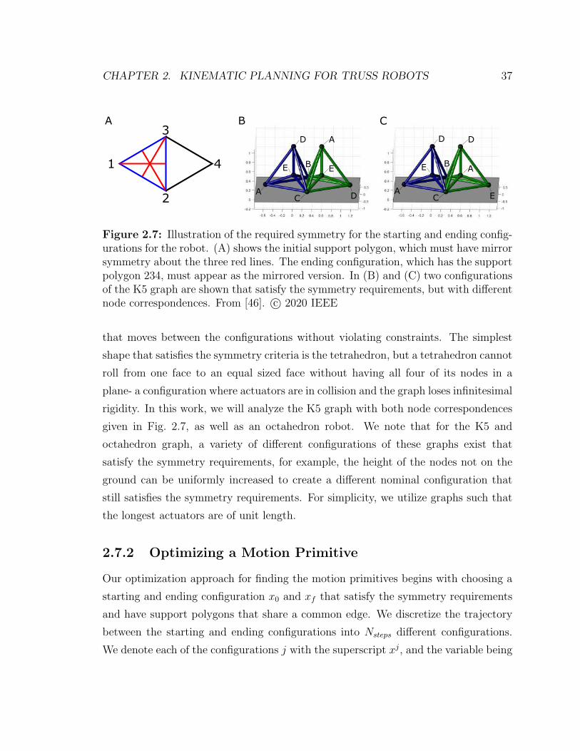
CHAPTER 2. KINEMATIC PLANNING FOR TRUSS ROBOTS 37
1
2
3
4
A
B
C D
AD
E E
A
B
C
D
E
E
D
A
A B C
Figure 2.7: Illustration of the required symmetry for the starting and ending config-urations for the robot. (A) shows the initial support polygon, which must have mirrorsymmetry about the three red lines. The ending configuration, which has the supportpolygon 234, must appear as the mirrored version. In (B) and (C) two configurationsof the K5 graph are shown that satisfy the symmetry requirements, but with differentnode correspondences. From [46]. c© 2020 IEEE
that moves between the configurations without violating constraints. The simplest
shape that satisfies the symmetry criteria is the tetrahedron, but a tetrahedron cannot
roll from one face to an equal sized face without having all four of its nodes in a
plane- a configuration where actuators are in collision and the graph loses infinitesimal
rigidity. In this work, we will analyze the K5 graph with both node correspondences
given in Fig. 2.7, as well as an octahedron robot. We note that for the K5 and
octahedron graph, a variety of different configurations of these graphs exist that
satisfy the symmetry requirements, for example, the height of the nodes not on the
ground can be uniformly increased to create a different nominal configuration that
still satisfies the symmetry requirements. For simplicity, we utilize graphs such that
the longest actuators are of unit length.
2.7.2 Optimizing a Motion Primitive
Our optimization approach for finding the motion primitives begins with choosing a
starting and ending configuration x0 and xf that satisfy the symmetry requirements
and have support polygons that share a common edge. We discretize the trajectory
between the starting and ending configurations into Nsteps different configurations.
We denote each of the configurations j with the superscript xj, and the variable being
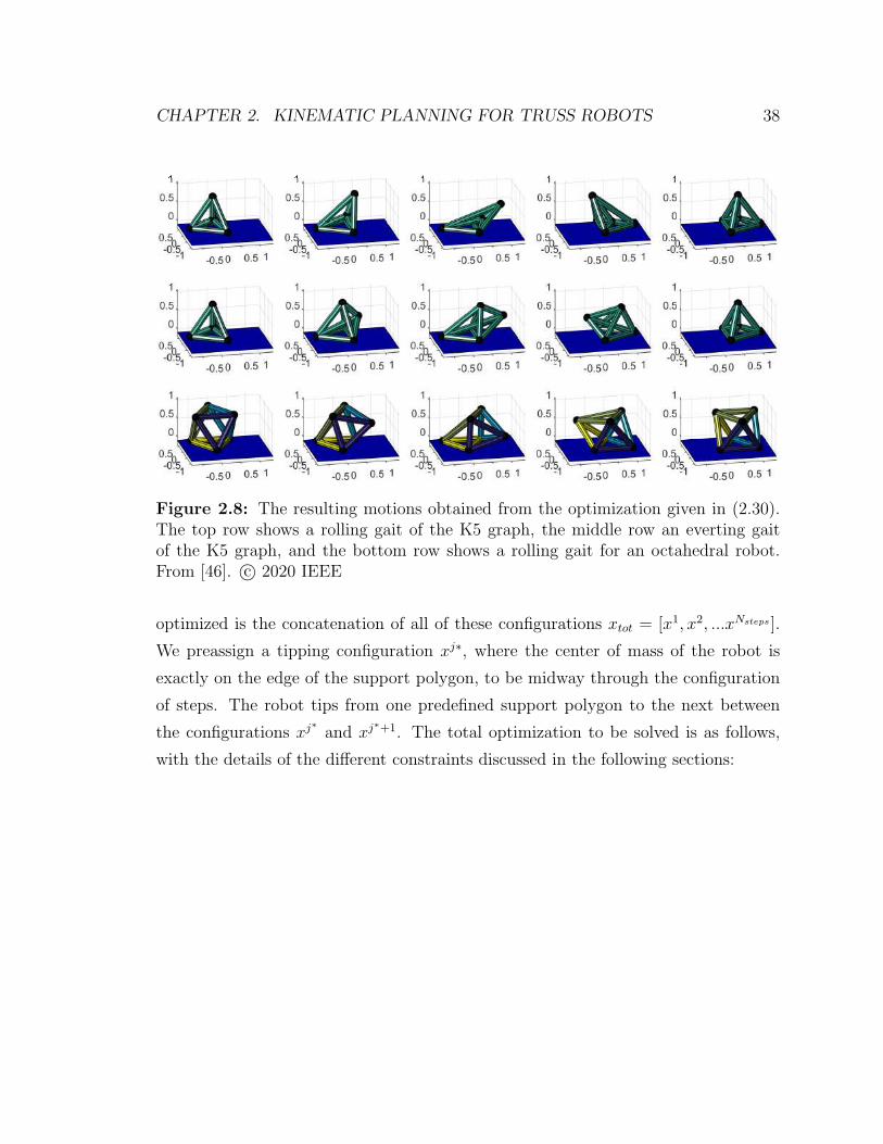
CHAPTER 2. KINEMATIC PLANNING FOR TRUSS ROBOTS 38
Figure 2.8: The resulting motions obtained from the optimization given in (2.30).The top row shows a rolling gait of the K5 graph, the middle row an everting gaitof the K5 graph, and the bottom row shows a rolling gait for an octahedral robot.From [46]. c© 2020 IEEE
optimized is the concatenation of all of these configurations xtot = [x1, x2, ...xNsteps ].
We preassign a tipping configuration xj∗, where the center of mass of the robot is
exactly on the edge of the support polygon, to be midway through the configuration
of steps. The robot tips from one predefined support polygon to the next between
the configurations xj∗
and xj∗+1. The total optimization to be solved is as follows,
with the details of the different constraints discussed in the following sections:
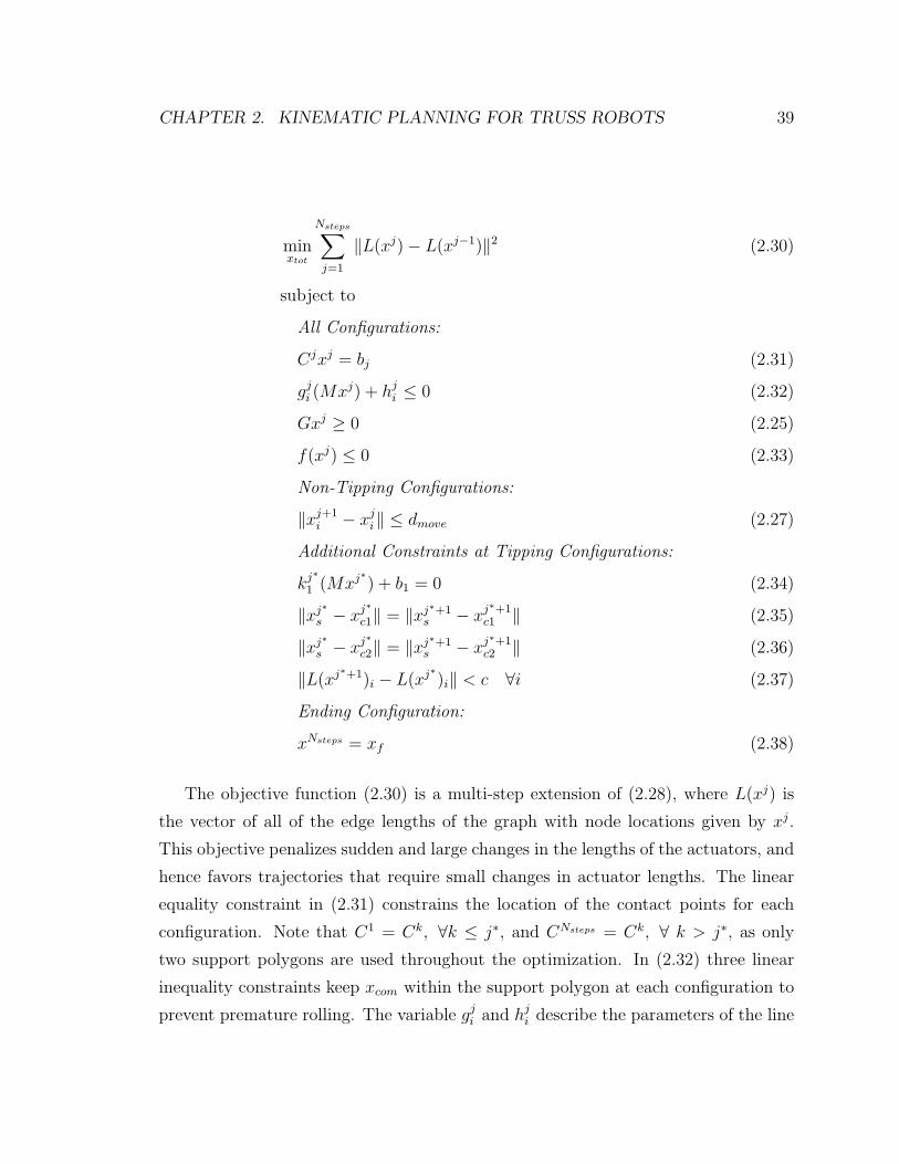
CHAPTER 2. KINEMATIC PLANNING FOR TRUSS ROBOTS 39
minxtot
Nsteps∑j=1
‖L(xj)− L(xj−1)‖2 (2.30)
subject to
All Configurations:
Cjxj = bj (2.31)
gji (Mxj) + hji ≤ 0 (2.32)
Gxj ≥ 0 (2.25)
f(xj) ≤ 0 (2.33)
Non-Tipping Configurations:
‖xj+1i − xji‖ ≤ dmove (2.27)
Additional Constraints at Tipping Configurations:
kj∗
1 (Mxj∗) + b1 = 0 (2.34)
‖xj∗s − xj∗
c1‖ = ‖xj∗+1s − xj
∗+1c1 ‖ (2.35)
‖xj∗s − xj∗
c2‖ = ‖xj∗+1s − xj
∗+1c2 ‖ (2.36)
‖L(xj∗+1)i − L(xj
∗)i‖ < c ∀i (2.37)
Ending Configuration:
xNsteps = xf (2.38)
The objective function (2.30) is a multi-step extension of (2.28), where L(xj) is
the vector of all of the edge lengths of the graph with node locations given by xj.
This objective penalizes sudden and large changes in the lengths of the actuators, and
hence favors trajectories that require small changes in actuator lengths. The linear
equality constraint in (2.31) constrains the location of the contact points for each
configuration. Note that C1 = Ck, ∀k ≤ j∗, and CNsteps = Ck, ∀ k > j∗, as only
two support polygons are used throughout the optimization. In (2.32) three linear
inequality constraints keep xcom within the support polygon at each configuration to
prevent premature rolling. The variable gji and hji describe the parameters of the line
CHAPTER 2. KINEMATIC PLANNING FOR TRUSS ROBOTS 40
along edge i of the support triangle. For each configuration, we denote f(xj) ≤ 0 to
represent all of the physical feasibility constraints for one configuration. We write the
constraint xNsteps = xf to ensure the proper final configuration.
We note that for the transition between the tipping configuration and the next
configuration (xj∗
and xj∗+1) large motions of the node positions are possible due to
the rolling, even though change in the edge lengths may be small. For the rolling
step alone, we constrain the change in edge lengths to be below a fixed threshold as
shown in (2.37) to prevent the robot from jumping over a physical constraint, such
as an actuator collision constraint, between configurations.
Tipping Constraints
In addition to the constraints that ensure that each configuration is feasible, we also
impose additional constraints that ensure that the robot tips at the predefined tipping
configuration. The linear equality constraint in (2.34) ensures that at the tipping
configuration the center of mass lie on the tipping edge of the support polygon. We
denote the new node in the support polygon after the tip as node s. The two quadratic
equality constraints in (2.35) and (2.36) ensure that the position of node s, denoted
xj∗s , is the proper distance away from each node on the rolling edge, denoted xj
∗
c1 and
xj∗
c2. Note that these constraints do not fix the height from which the robot tips onto
the next support polygon. Were the height and position of the next point specified
exactly, the two quadratic constraints would be replaced by three linear constraints,
but the optimization would lose the ability to change the tipping height.
Optimization Results
The motion primitives produced by solving the optimization problem are shown in
Fig. 2.8. For these results, we use Nsteps = 40, with the tipping configuration j∗ =
20. We initialize the optimization such that every configuration or after the tipping
configuration is exactly the starting or ending configuration respectively. We initialize
the tipping configuration with, all nodes of the initial and final support polygon in
place, and the nodes that are not part of the support polygon positioned such that
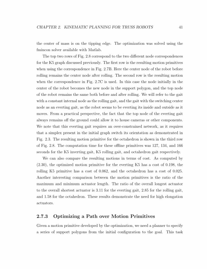
CHAPTER 2. KINEMATIC PLANNING FOR TRUSS ROBOTS 41
the center of mass is on the tipping edge. The optimization was solved using the
fmincon solver available with Matlab.
The top two rows of Fig. 2.8 correspond to the two different node correspondences
for the K5 graph discussed previously. The first row is the resulting motion primitives
when using the correspondence in Fig. 2.7B. Here the center node of the robot before
rolling remains the center node after rolling. The second row is the resulting motion
when the correspondence in Fig. 2.7C is used. In this case the node initially in the
center of the robot becomes the new node in the support polygon, and the top node
of the robot remains the same both before and after rolling. We will refer to the gait
with a constant internal node as the rolling gait, and the gait with the switching center
node as an everting gait, as the robot seems to be everting its inside and outside as it
moves. From a practical perspective, the fact that the top node of the everting gait
always remains off the ground could allow it to house cameras or other components.
We note that this everting gait requires an over-constrained network, as it requires
that a simplex present in the initial graph switch its orientation as demonstrated in
Fig. 2.3. The resulting motion primitive for the octahedron is shown in the third row
of Fig. 2.8. The computation time for these offline primitives was 127, 134, and 166
seconds for the K5 inverting gait, K5 rolling gait, and octahedron gait respectively.
We can also compare the resulting motions in terms of cost. As computed by
(2.30), the optimized motion primitive for the everting K5 has a cost of 0.198, the
rolling K5 primitive has a cost of 0.062, and the octahedron has a cost of 0.025.
Another interesting comparison between the motion primitives is the ratio of the
maximum and minimum actuator length. The ratio of the overall longest actuator
to the overall shortest actuator is 3.11 for the everting gait, 2.85 for the rolling gait,
and 1.58 for the octahedron. These results demonstrate the need for high elongation
actuators.
2.7.3 Optimizing a Path over Motion Primitives
Given a motion primitive developed by the optimization, we need a planner to specify
a series of support polygons from the initial configuration to the goal. This task

CHAPTER 2. KINEMATIC PLANNING FOR TRUSS ROBOTS 42
Figure 2.9: An example of the A* planning algorithm. The black boxes are obsta-cles, the red triangles the closed set (reachable configurations explored by A*), andthe green triangles the open set (configurations that the planner will consider addingto the closed set). From [46]. c© 2020 IEEE
corresponds to planning a path on a triangular grid of candidate support polygons.
We use the A* algorithm for this task, but note that any discrete planning algorithm
could be used for this task. An example of A* finding a path through obstacles is
shown in Fig. 2.9. If a feasible trajectory is found that solves the optimization and a
feasible path is found between the starting configuration and the goal region, a feasible
path that satisfies all constraints is possible from the start to the goal region. Note
that in the case of an environment with obstacles, the collision checking performed
as part of the A* algorithm depends in part on the robot gait. The maximum extent
of the computational gait must be used by the planner to ensure that it is possible
to move from one support polygon to another. If a path of collision free support
polygons that leads from the start to the goal exists, the A* algorithm is guaranteed
to find it. However, it is possible that if A* fails to find a path, the robot could pass
through the environment by using a different motion primitive.
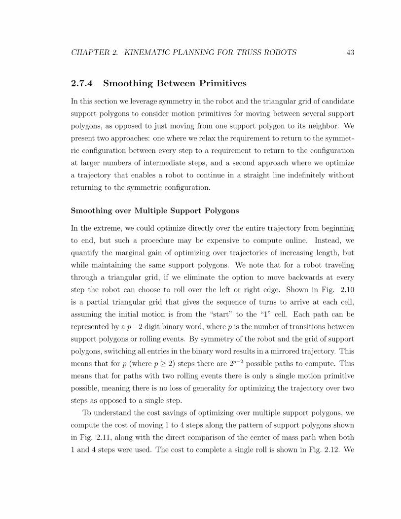
CHAPTER 2. KINEMATIC PLANNING FOR TRUSS ROBOTS 43
2.7.4 Smoothing Between Primitives
In this section we leverage symmetry in the robot and the triangular grid of candidate
support polygons to consider motion primitives for moving between several support
polygons, as opposed to just moving from one support polygon to its neighbor. We
present two approaches: one where we relax the requirement to return to the symmet-
ric configuration between every step to a requirement to return to the configuration
at larger numbers of intermediate steps, and a second approach where we optimize
a trajectory that enables a robot to continue in a straight line indefinitely without
returning to the symmetric configuration.
Smoothing over Multiple Support Polygons
In the extreme, we could optimize directly over the entire trajectory from beginning
to end, but such a procedure may be expensive to compute online. Instead, we
quantify the marginal gain of optimizing over trajectories of increasing length, but
while maintaining the same support polygons. We note that for a robot traveling
through a triangular grid, if we eliminate the option to move backwards at every
step the robot can choose to roll over the left or right edge. Shown in Fig. 2.10
is a partial triangular grid that gives the sequence of turns to arrive at each cell,
assuming the initial motion is from the “start” to the “1” cell. Each path can be
represented by a p−2 digit binary word, where p is the number of transitions between
support polygons or rolling events. By symmetry of the robot and the grid of support
polygons, switching all entries in the binary word results in a mirrored trajectory. This
means that for p (where p ≥ 2) steps there are 2p−2 possible paths to compute. This
means that for paths with two rolling events there is only a single motion primitive
possible, meaning there is no loss of generality for optimizing the trajectory over two
steps as opposed to a single step.
To understand the cost savings of optimizing over multiple support polygons, we
compute the cost of moving 1 to 4 steps along the pattern of support polygons shown
in Fig. 2.11, along with the direct comparison of the center of mass path when both
1 and 4 steps were used. The cost to complete a single roll is shown in Fig. 2.12. We
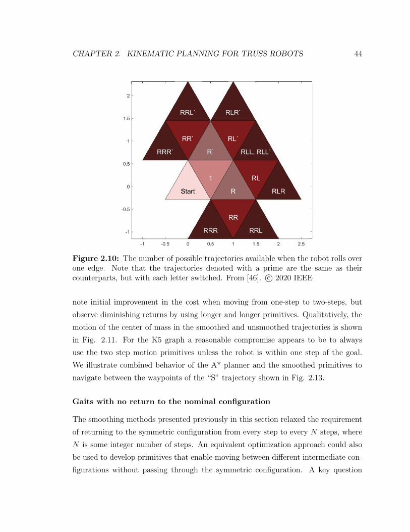
CHAPTER 2. KINEMATIC PLANNING FOR TRUSS ROBOTS 44
Figure 2.10: The number of possible trajectories available when the robot rolls overone edge. Note that the trajectories denoted with a prime are the same as theircounterparts, but with each letter switched. From [46]. c© 2020 IEEE
note initial improvement in the cost when moving from one-step to two-steps, but
observe diminishing returns by using longer and longer primitives. Qualitatively, the
motion of the center of mass in the smoothed and unsmoothed trajectories is shown
in Fig. 2.11. For the K5 graph a reasonable compromise appears to be to always
use the two step motion primitives unless the robot is within one step of the goal.
We illustrate combined behavior of the A* planner and the smoothed primitives to
navigate between the waypoints of the “S” trajectory shown in Fig. 2.13.
Gaits with no return to the nominal configuration
The smoothing methods presented previously in this section relaxed the requirement
of returning to the symmetric configuration from every step to every N steps, where
N is some integer number of steps. An equivalent optimization approach could also
be used to develop primitives that enable moving between different intermediate con-
figurations without passing through the symmetric configuration. A key question
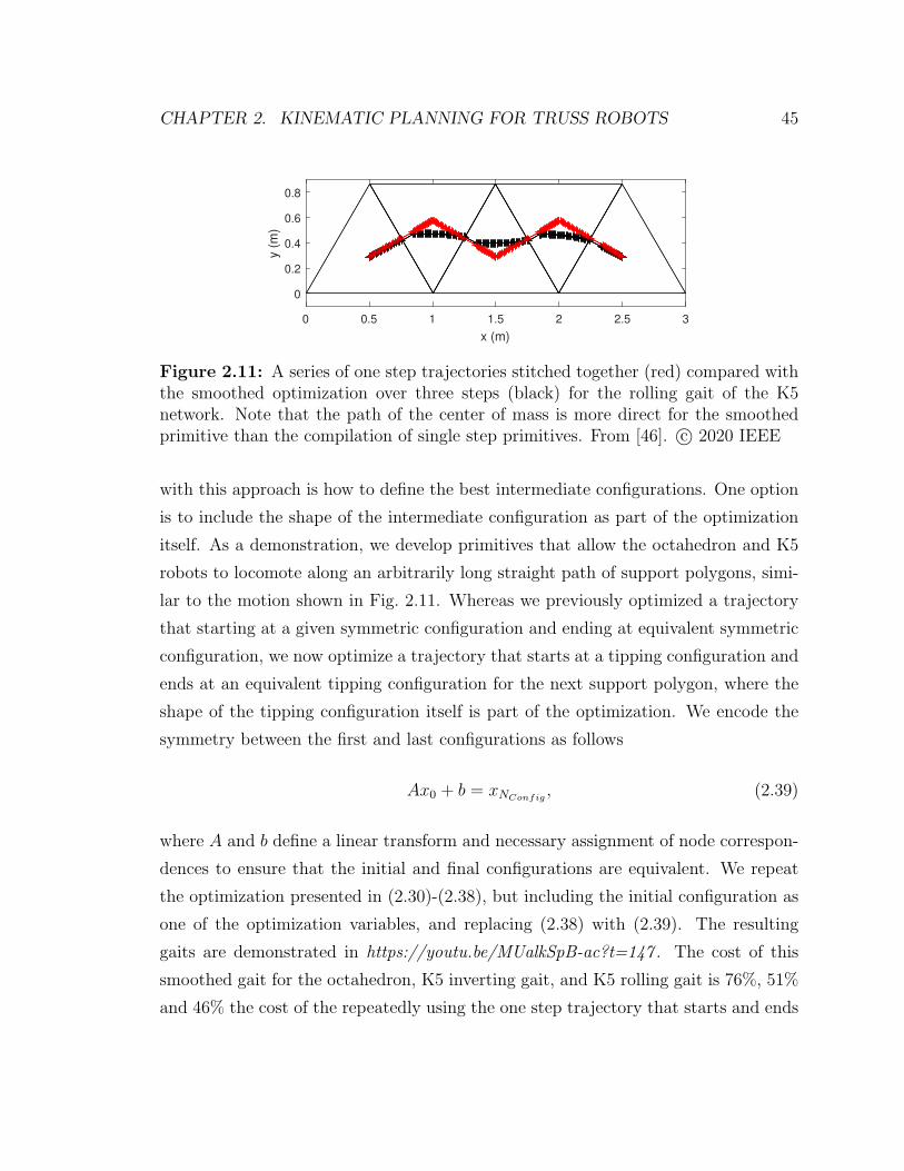
CHAPTER 2. KINEMATIC PLANNING FOR TRUSS ROBOTS 45
0 0.5 1 1.5 2 2.5 3
x (m)
0
0.2
0.4
0.6
0.8
y (
m)
Figure 2.11: A series of one step trajectories stitched together (red) compared withthe smoothed optimization over three steps (black) for the rolling gait of the K5network. Note that the path of the center of mass is more direct for the smoothedprimitive than the compilation of single step primitives. From [46]. c© 2020 IEEE
with this approach is how to define the best intermediate configurations. One option
is to include the shape of the intermediate configuration as part of the optimization
itself. As a demonstration, we develop primitives that allow the octahedron and K5
robots to locomote along an arbitrarily long straight path of support polygons, simi-
lar to the motion shown in Fig. 2.11. Whereas we previously optimized a trajectory
that starting at a given symmetric configuration and ending at equivalent symmetric
configuration, we now optimize a trajectory that starts at a tipping configuration and
ends at an equivalent tipping configuration for the next support polygon, where the
shape of the tipping configuration itself is part of the optimization. We encode the
symmetry between the first and last configurations as follows
Ax0 + b = xNConfig, (2.39)
where A and b define a linear transform and necessary assignment of node correspon-
dences to ensure that the initial and final configurations are equivalent. We repeat
the optimization presented in (2.30)-(2.38), but including the initial configuration as
one of the optimization variables, and replacing (2.38) with (2.39). The resulting
gaits are demonstrated in https://youtu.be/MUalkSpB-ac?t=147 . The cost of this
smoothed gait for the octahedron, K5 inverting gait, and K5 rolling gait is 76%, 51%
and 46% the cost of the repeatedly using the one step trajectory that starts and ends

CHAPTER 2. KINEMATIC PLANNING FOR TRUSS ROBOTS 46
1 2 3 4
Number of Rolls
0
0.05
0.1
0.15
0.2
0.25
0.3
0.35
Cost P
er
Roll
Inverting Gait
Rolling Gait
Figure 2.12: A comparison of the cost per roll when optimized over multiple rolls.The cost per roll is monotonically decreasing. From [46]. c© 2020 IEEE
in the symmetric configuration, representing a substantial savings. Utilizing these
gaits online in the robot requires storing the repeating gait as well as the trajectory
to move to and from the symmetric configuration to be used at the beginning and
end of the straight line trajectory. This means that the memory required to store this
gait is equivalent to the memory required to store a two-roll primitive. Due to the
cost to move from the initial configuration to the rolling configuration, the multi-step
primitives such as those shown in Fig. 2.11 are superior for short sequences of support
polygons. However, as the length of the trajectory increases, the cost of using the
repeated gaits approaches the cost obtained by optimizing over the entire trajectory,
but requires a smaller amount of memory to store. Future work could seek to define
intermediate gaits and other shapes that enable different behaviors such as turning.
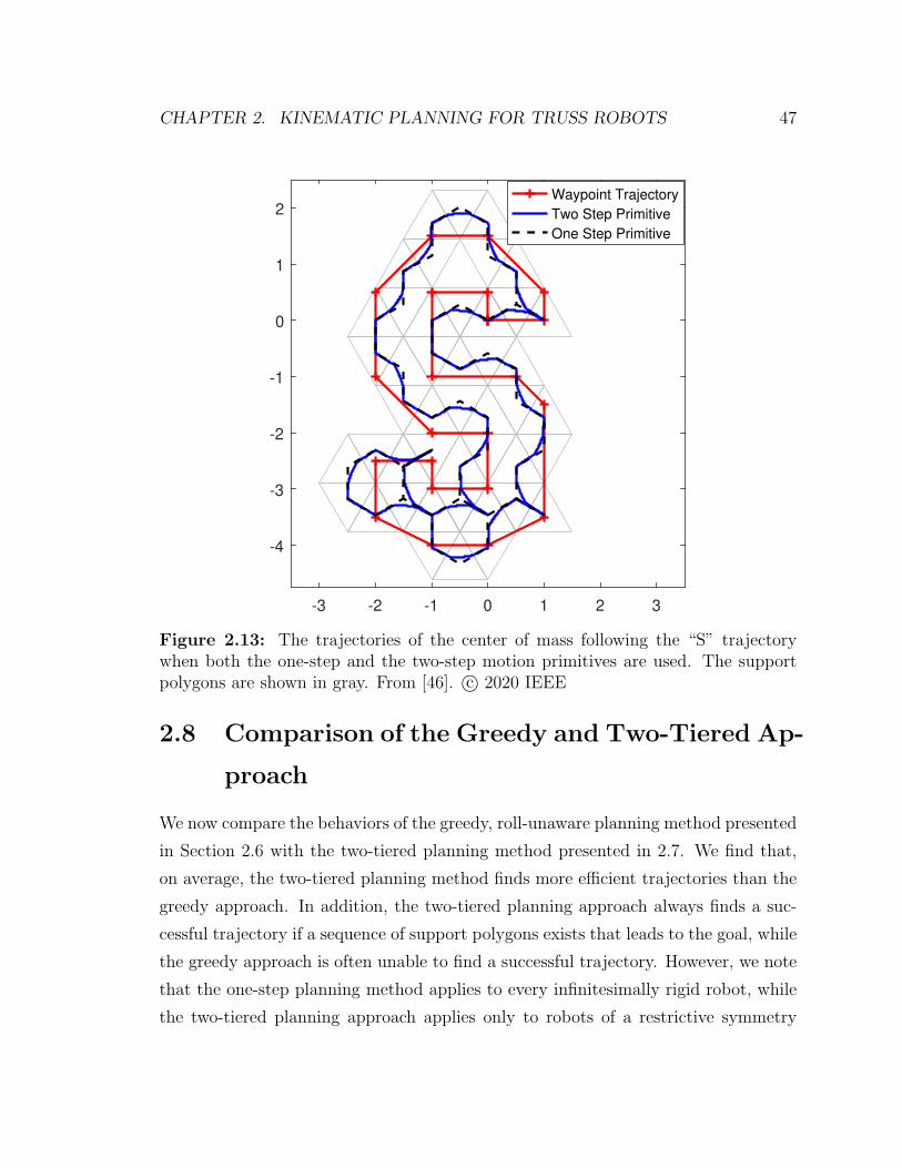
CHAPTER 2. KINEMATIC PLANNING FOR TRUSS ROBOTS 47
-3 -2 -1 0 1 2 3
-4
-3
-2
-1
0
1
2Waypoint Trajectory
Two Step Primitive
One Step Primitive
Figure 2.13: The trajectories of the center of mass following the “S” trajectorywhen both the one-step and the two-step motion primitives are used. The supportpolygons are shown in gray. From [46]. c© 2020 IEEE
2.8 Comparison of the Greedy and Two-Tiered Ap-
proach
We now compare the behaviors of the greedy, roll-unaware planning method presented
in Section 2.6 with the two-tiered planning method presented in 2.7. We find that,
on average, the two-tiered planning method finds more efficient trajectories than the
greedy approach. In addition, the two-tiered planning approach always finds a suc-
cessful trajectory if a sequence of support polygons exists that leads to the goal, while
the greedy approach is often unable to find a successful trajectory. However, we note
that the one-step planning method applies to every infinitesimally rigid robot, while
the two-tiered planning approach applies only to robots of a restrictive symmetry
CHAPTER 2. KINEMATIC PLANNING FOR TRUSS ROBOTS 48
class.
Conceptually, we can compare the behavior of the two planners by comparing
the resulting center of mass trajectories in Fig. 2.5 and Fig. 2.13. With the two
tiered planning approach, the trajectory of the center of mass takes a less direct
path between waypoints, as the constraint to move the support polygon along the
triangular grid ensures that the center of mass does not move in a straight line.
Despite the apparent inefficiency of the trajectory from the two-tiered planner, we
find that it results in lower cost trajectories. We hypothesize that this occurs because
the robot remains in a better conditioned state. The two-tiered planner generates
trajectories with consistent motion of all of the free nodes, while in the trajectories
of the greedy planner free nodes seem to be flailing about a relatively steady center
of mass trajectory.
For a quantitative comparison of the performance of the planners, we generated
100 sequences of 5 random waypoints in a 5 unit by 5 unit region and use the proposed
planning methods to find a trajectory to visit the waypoints sequentially. As the
output of the optimization is a kinematic trajectory, we scale the trajectories such
that completing the entire trajectory takes 1 unit of time, and convert the trajectory
to continuous time by linearly interpolating the node positions between the discrete
configurations returned by the optimization. This rescaling ensure an equivalent
average velocity between the different experiments, and allows a direct comparison in
terms of the cost. To evaluate the cost of the trajectories we use the following cost
function:
J =
∫ 1
0‖L(x(t))‖2dt
d(2.40)
where d is the sum of the straight line distances between the waypoints. This cost is
a continuous time version of (2.28), divided by the path length to give an efficiency
metric as the average cost to move a unit distance. Using both the K5 and the
octahedron robot, Fig. 2.14 compares the efficiency of the paths resulting from the
two-tiered planning method (using both the rolling and everting primitive for the K5
graph), and the greedy method using both (2.28) and (2.29) as the objective. For both

CHAPTER 2. KINEMATIC PLANNING FOR TRUSS ROBOTS 49
the octahedron and the K5 graph, the two-tiered planning approach attains lower cost
and lower variance than the greedy approach for the same robot. Interestingly, for
both the octahedron and the K5 graph, a lower overall cost is obtained by using
(2.29), the cost function that penalizes actuator for deviating from a nominal length,
as the cost as opposed to (2.28), which penalizes changes in actuator length at each
time step and is the single-step version of (2.40). This seems to indicate that long
term efficiency is achieved by keeping the robot in a relatively well-conditioned state.
In addition to cost, the other key criteria by which to evaluate the planners is their
ability to find a complete path without violating constraints. For the 100 randomly
generated trajectories and using the K5 robot, the one-step optimization method
successfully found a path between all waypoints for 12% of the trials when using
(2.28) as the objective, and for 70% of the trials when using the formation-control
based objective given in (2.29). We repeated the experiments with the octahedron,
and found convergence occurred for 85% of the trajectories when using the objective
in (2.28), and 75% when using the objective in (2.29). Interestingly, for the K5
graph the formation objective (2.29) leads to more frequent convergence than the
minimum norm objective (2.28), but for the octahedron the results are reversed.
The most common failure mode for the K5 graph is rolling onto a support polygon
with extremely long actuator lengths between the support nodes, and then being
unable to move the remaining nodes far enough to cause a tip without violating
constraints. The use of the formation objective that seeks to keep the edge lengths at a
nominal operating point tends to avoid this scenario. For the octahedron, failure most
commonly occurred through inability to satisfy the rigidity maintenance constraint.
The approximately equal edge lengths favored by the formation objective seem to be
slightly more likely to put the robot into a configuration with low rigidity.
The two-tiered planning approach has the valuable guarantee of persistent feasibil-
ity and performs better than the one step method in terms of cost, probably because
the robot remains in a relatively well conditioned state throughout the motion. How-
ever, this method only applies to robots that meet strict symmetry requirements.
The one-step method is general to any infinitesimally rigid robot, but contains no
guarantee of persistent feasibility.
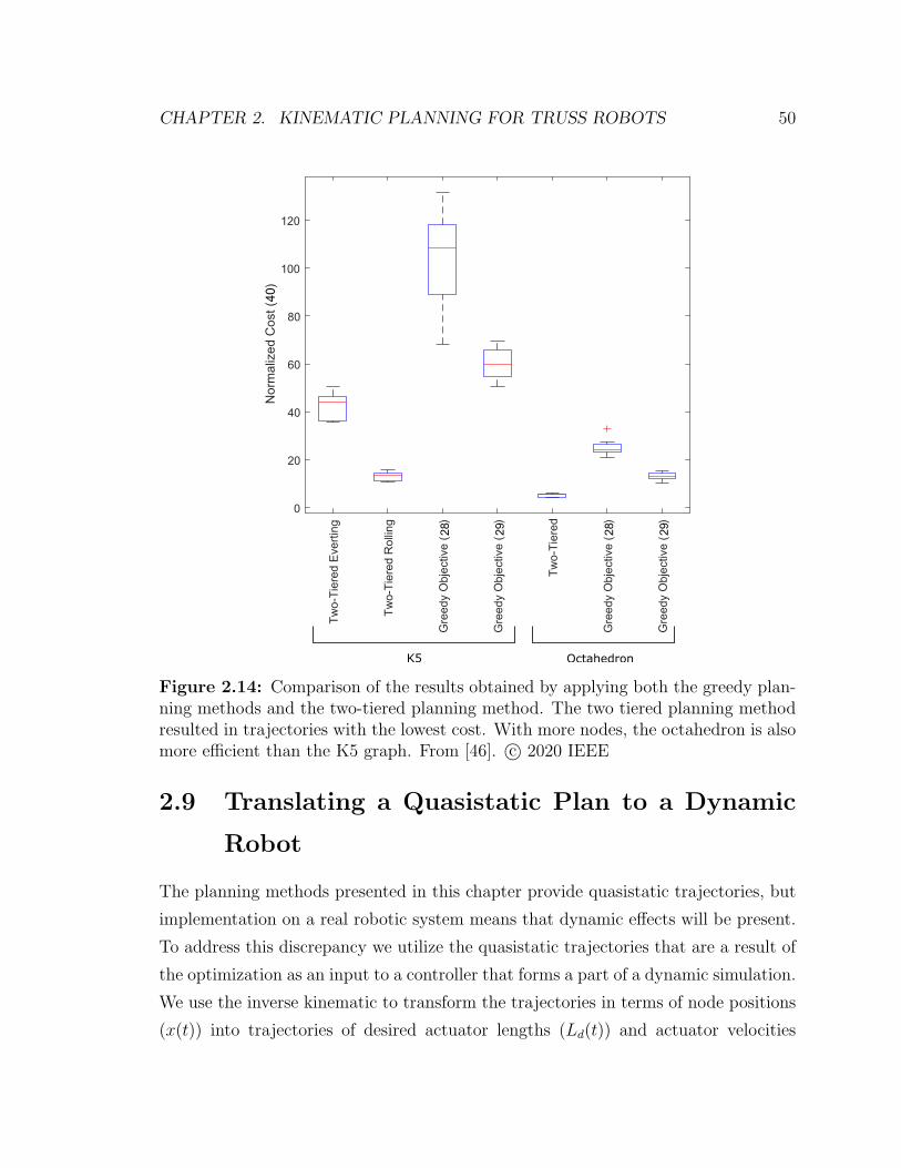
CHAPTER 2. KINEMATIC PLANNING FOR TRUSS ROBOTS 50
Tw
o-T
iere
d E
vert
ing
Tw
o-T
iere
d R
ollin
g
Gre
edy
Obj
ectiv
e (
)
Gre
edy
Obj
ectiv
e (
)
Tw
o-T
iere
d
Gre
edy
Obj
ectiv
e (
)
Gre
edy
Obj
ectiv
e (
)
0
20
40
60
80
100
120
Nor
mal
ized
Cos
t ()
40
28 29 28 29K5 Octahedron
Figure 2.14: Comparison of the results obtained by applying both the greedy plan-ning methods and the two-tiered planning method. The two tiered planning methodresulted in trajectories with the lowest cost. With more nodes, the octahedron is alsomore efficient than the K5 graph. From [46]. c© 2020 IEEE
2.9 Translating a Quasistatic Plan to a Dynamic
Robot
The planning methods presented in this chapter provide quasistatic trajectories, but
implementation on a real robotic system means that dynamic effects will be present.
To address this discrepancy we utilize the quasistatic trajectories that are a result of
the optimization as an input to a controller that forms a part of a dynamic simulation.
We use the inverse kinematic to transform the trajectories in terms of node positions
(x(t)) into trajectories of desired actuator lengths (Ld(t)) and actuator velocities
CHAPTER 2. KINEMATIC PLANNING FOR TRUSS ROBOTS 51
(Ld(t)), and then utilize a simple PID controller to compute the force (τ(t)) to be
applied by each actuator as follows,
τ(t) = Kpe(t) +Kde(t) +KI
∫ t
0
e(t)dt, (2.41)
where e(t) = L(t)− Ld(t).For this controller, the robot only has knowledge of the lengths of its actuators, and
requires no knowledge of the position of its nodes in space. For this proof-of-concept
implementation, we assume that each actuator can be approximated as having half
of its mass at each node. Knowing the forces applied by the actuator, we determine
the forces on each node as follows:
Mx = Ftot =[R(x)T CT
] [τ(t)
E(t)
]+ Fext, (2.42)
Where E(t) are the ground reaction forces and Fext are the external forces applied
on the robot, which in this case is the gravity acting on each node. We solve for E(t)
such that the resultant force (Ftot) on the ground nodes are equal to 0. Rolling occurs
when the reaction force at any ground node is negative in the vertical direction. When
his occurs, we remove the node from the support polygon (and the corresponding
constraints from the C matrix) and continue propagating the dynamics until a new
node makes contact with the ground. We assume that all collisions with the ground
are perfectly inelastic, meaning that the velocity of the node that contacts the ground
immediately becomes 0. We use Matlab ode45 to perform the dynamic simulation.
To evaluate our system, we utilize the gaits shown in Fig. 2.8 as inputs to the PID
controller. The videos of the simulated dynamics are shown at ://youtu.be/MUalkSpB-
ac?t=85. For these simulations, we assume that the initial length of the longest ac-
tuator in each robot has a length of 1 m, and that each node has a mass of 1 kg. To
evaluate the gaits, we compute the average error between the nodes in the dynamic
simulation and their expected location from the quasistatic plan. As the quasistatic
gaits do not account for the rolling behavior, we do not compute the error for the por-
tion of the trajectory where only two nodes of the dynamic robot are on the ground.
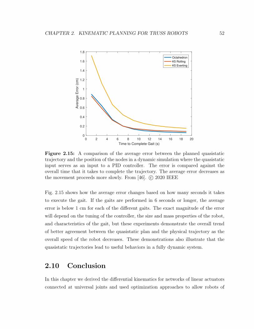
CHAPTER 2. KINEMATIC PLANNING FOR TRUSS ROBOTS 52
0 2 4 6 8 10 12 14 16 18 20
Time to Complete Gait (s)
0
0.2
0.4
0.6
0.8
1
1.2
1.4
1.6
1.8
Ave
rag
e E
rro
r (c
m)
Octahedron
K5 Rolling
K5 Everting
Figure 2.15: A comparison of the average error between the planned quasistatictrajectory and the position of the nodes in a dynamic simulation where the quasistaticinput serves as an input to a PID controller. The error is compared against theoverall time that it takes to complete the trajectory. The average error decreases asthe movement proceeds more slowly. From [46]. c© 2020 IEEE
Fig. 2.15 shows how the average error changes based on how many seconds it takes
to execute the gait. If the gaits are performed in 6 seconds or longer, the average
error is below 1 cm for each of the different gaits. The exact magnitude of the error
will depend on the tuning of the controller, the size and mass properties of the robot,
and characteristics of the gait, but these experiments demonstrate the overall trend
of better agreement between the quasistatic plan and the physical trajectory as the
overall speed of the robot decreases. These demonstrations also illustrate that the
quasistatic trajectories lead to useful behaviors in a fully dynamic system.
2.10 Conclusion
In this chapter we derived the differential kinematics for networks of linear actuators
connected at universal joints and used optimization approaches to allow robots of

CHAPTER 2. KINEMATIC PLANNING FOR TRUSS ROBOTS 53
this type to move coordinate their many degrees of freedom to locomote. We have
shown that if the embedded graph describing the robot is infinitesimally rigid, any
desired motion of the nodes can be achieved through some motion of the edges. We
then framed the locomotion problem as a nonlinear optimization over the node posi-
tions, while enforcing constraints that guarantee the feasibility of the robot. We also
discussed that constraints to maintain the infinitesimal rigidity of the robot tend to
divide the state space of the robot into separated regions, even though the singular
configurations themselves make up a set of zero measure. We discussed the control
of both minimally rigid graphs and over-constrained graphs, and demonstrated that
over-constrained graphs can achieve some behaviors that minimally rigid graphs can-
not, such as the everting locomotion gait of the K5 graph. We present two planning
schemes: one where we solve a single step nonlinear optimization online to achieve
a desired instantaneous motion of the center of mass, and another where we opti-
mize over many configurations that compose a motion primitive, including in the
optimization direct consideration of the rolling behavior. The single-step approach is
applicable to robots of arbitrary configuration, but there is the possibility that the
robot will reach a state from which it cannot continue in the desired direction with-
out violating physical constraints. While these is no guarantee of persistent feasibility
with this approach, we have found that long trajectories can be achieved based on
the choice of the cost function. The two-tiered approach ensures persistent feasibility,
but requires the robot to satisfy certain symmetry properties. The techniques devel-
oped in this chapter allow for the control of the any infinitesimally rigid truss robot
through control of the edge lengths.

Chapter 3
An Untethered Isoperimetric Soft
Robot
3.1 Introduction
For robots to work in conjunction with humans and be useful outside of highly en-
gineered environments, they must be human-safe, robust, adaptable to a variety of
scenarios, and capable of moving through diverse types of terrain. These attributes
require not only adaptable control algorithms and the collection and processing of
rich sensory information, but also new forms of reconfigurable, adaptable robotic
structures, which are potentially soft in nature. The previous chapter focused on
control algorithms that enable truss robots to perform useful tasks. This chapter dis-
cusses the design and control of a novel type of truss robot that demonstrates useful
behaviors in the real world.
We present a concept for an adaptable, human-safe robotic structure: a truss of
inextensible, inflatable, constant-length tubes that are manipulated by a collective
of interconnected roller modules, allowing for shape change and compliance without
a pressure source (Fig. 3.1). Pressurized tubes serve as structural elements and the
edges of the truss. Each joint in the tubing is formed by a robotic roller module
that pinches the tube between cylindrical rollers without creating a seal. The roller
54

CHAPTER 3. AN UNTETHERED ISOPERIMETRIC SOFT ROBOT 55
Figure 3.1: A soft isoperimetric robot. (A) An overview of the human scale robotthat is composed of inflated fabric tubes that pass through roller modules. (B) A closeup of a roller module. (C) Illustration of how the roller modules moves along the tube,simultaneously lengthening one edges and shortening another while maintaining thetotal edge length. Modified from [13] with permission from AAAS.
modules can be connected to neighboring modules to form a node of a complex two-
dimensional (2D) or 3D structure. An electric motor and mechanical transmission
then drive these rollers like wheels along the tube, causing the pinch point to translate
(Fig. 3.1B). Edge lengths of the robot are changed not by stretching or contracting
the edges but by movement of the roller module along the tube — moving the effective
joint and simultaneously lengthening one edge while shortening another (Fig. 3.1C).
The sum of all the edge lengths remains constant; therefore, we call the robot an
isoperimetric system (constant perimeter). A gap between the rollers ensures that as
they move, there is negligible pressure difference between the two edges, leading to a
system with constant volume that does not require a pressure source. The individual
roller modules can connect to other modules through a universal joint Fig. 3.1(D) and
are capable of moving along the tube in only one degree of freedom, yet the overall
collective is capable of complex behavior (Fig. 3.1E).
This chapter is organized as follows. We first present related work on truss robots,

CHAPTER 3. AN UNTETHERED ISOPERIMETRIC SOFT ROBOT 56
untethered soft robots, and collective robots. We then present models and experi-
ments that inform the mechanical design of the roller modules that make up the
robot. Next we extend the kinematic model from the previous chapter to the case
where the total edge length of the robot must be conserved. We then present nu-
merous demonstrations to highlight the collective, truss-like, and soft nature of our
robots. To highlight the collective and modular nature of the robot, we present three
different robots, two 2D robots and one 3D robot, each constructed from identical
one-degree-of-freedom roller modules, yet as a collective, capable of complex move-
ment. To demonstrate the truss-like nature of the robot, we show marked shape
change of all three of the robots and punctuated rolling locomotion of the 3D robot.
To demonstrate and characterize the softness of the robot, we show its robustness
to crushing forces, measure its behavior under load, and leverage its compliance to
grasp and manipulate objects. Each of these demonstrations is conducted with the
robot untethered from a pressure source. We conclude by presenting tradeoffs among
isoperimetric truss robots, conventional truss robots, and pneumatically actuated
robots. This chapter was completed in close collaboration with Zachary Hammond,
and who was co-first author for the paper on which this chapter is based [13].
3.2 Related Work
The development of isoperimetric robots draws from work on truss robots, collective
robots and soft robots. Many of the proposed applications and past instantiations
of truss robots have been presented in Chapter 1. The mechanical design of these
systems focuses primarily on design of actuators [30,31], design of universal joints, or
the design of both components [28, 29]. In a conventional truss robot, the edges of
the structure provide both the structure and the means of actuation. Our approach
is different in that the nodes provide the actuation, and the edges of the structure are
a set of inflated fabric tubes that can be continuously deformed by the joints. The
inflated structure of the robot gives it compliance, but the fact that the total amount
of air is constant means that no air source is required. This overcomes many of the
limitations of different pneumatic sources presented in the Chapter 1 and reviewed
CHAPTER 3. AN UNTETHERED ISOPERIMETRIC SOFT ROBOT 57
in [12]. This approach is similar to other soft robotic systems that use a fixed amount
of air within a cavity as a structural element and not as an actuator, requiring no
pressure source once the cavity is pressurized [77,78,79,80,81,82]. Some of this work
has exhibited direct manipulation of the membrane of an inflated beam to create
bending without compressing the air within [78,79]. We built upon this work for our
soft, untethered robot, but instead of manipulating a serial robot by deforming the
membrane around fixed joints as in [78,79], we continuously move the effective joints
along the structure, which allows large, global shape change of a truss-like robot.
As a collective system of robots, our concept is inherently modular with inter-
changeable, simple (one-degree-of-freedom) subunit roller modules. However, because
our subunits are physically interconnected through a compliant network, the collective
achieves complex system-level behavior, capable of applying forces in three dimen-
sions on a large scale. This overcomes a limitation of collective robots that combine
together to create structures that can change their shape [43, 44, 83, 84]— realizing
complex 3D physical interaction while maintaining simplicity at the individual robot
level. A related type of collective robotic system uses teams of robots that build pas-
sive structures [85,86,87,88]. The target structure is often truss-like, built by adding
passive elements, and sometimes requires that the robots traverse the structure as
they build it. Rather than discretely rearranging passive elements within a structure
to change its shape, in our concept, the collective continuously deforms the compliant
passive elements, resulting in very simple robotic subunits.
3.3 Roller Module Design and Analysis
The key components of our robot are the tubes and the actuated roller modules,
shown in Fig. 3.1. Each roller module in the robot serves three primary functions:
(i) to pinch the tube, creating a region of low bending stiffness—an effective joint;
(ii) to locomote along the length of the tube, moving the position of the effective
joint; and (iii) to mechanically couple to other roller modules in the structure in a
way that fully defines the geometry of the robot. In this section we discuss models
and experiments that examine each of these functions, and which contribute to the
CHAPTER 3. AN UNTETHERED ISOPERIMETRIC SOFT ROBOT 58
roller module design. We conclude this section by presenting the design utilized for
this robot.
3.3.1 Joint-Like Behavior of a Pinched Tube
In this section we develop a model of the effective joints of the structure which we
then validate experimentally. The effective joints, about which two sections of an
inflated tube pivot, are created by the cylindrical rollers in the roller modules. The
rollers pinch the tube, reducing its cross-sectional area and bending stiffness while
still allowing airflow. Ideally, there would be no torque required to change the angle,
but in practice, there is a torque at these joints. To understand and minimize this
torque, we developed a reduced order model. We assume that the fabric that makes
up the pressurized tube is flexible yet inextensible and takes a shape that maximizes
the enclosed volume, independent of its material properties or internal pressure. This
means that the volume enclosed by the fabric tube is a function of the the angle of
the tube (V = f(θ)), and not a function of the pressure. We relate the torque applied
by the joint τ to the internal pressure P and the change in volume with angle dV (θ)dθ
using the principle of virtual work through
τ = PdV (θ)
dθ(3.1)
Using this model requires us to (i) parameterize the shape of the tube, (ii) compute
the tube’s volume, and (iii) characterize the change in volume with angle. Past
work has studied the post-buckling bending response of inflated fabric beams without
rollers [89, 90], as well as models to predict the force exerted on the rollers when the
tube is only inflated on one side of the rollers [91, 92]. Our approach will combine
elements of these modeling approaches to quantify the change in torque with the
angle of a beam passing through a set of rollers.
Shape Parameterization
We parameterize the shape of the tube as shown in Fig. 3.2A. We assume that the
paths along the top and bottom of the inflated membrane are of equal length, smooth

CHAPTER 3. AN UNTETHERED ISOPERIMETRIC SOFT ROBOT 59
A
h
Rroll
D
θctop
cbottom
Rtop
Rbottom
αbottom
αtop
htube
Tube Cross Section
Connection to pressure
regulator
Mark 10 Force Sensor
Rollers
Brace to Hold Tube
In�ated Fabric TubeC
B
αtop θ
αbottom
θ
-10 0 10-10
-5
0
5
y (c
m)
-10 0 10
x (cm)
-10
-5
0
5
-10 0 10-10
-5
0
5
Figure 3.2: (A) Parameterization of the resulting shape of the tube as it passesthrough the rollers. We assume that the top and bottom path along the tube takea continuous path with two constant curvature segments. (B) The optimized shapesof the tube when straight, at an intermediate angle, and at the configuration wherethe membrane begins to self-intersect. (C) The test setup used to collect the data weused to compare with the model. Reprinted from [13] with permission from AAAS.
(the derivative is continuous everywhere), and that they are composed of a constant
curvature section and a straight section when not in contact with the roller. We wish
to express the equation of the top and bottom paths as functions of the geometric
constant parameters (D, h, Rroll, Ltot, θ), and two input parameters of our choice
that we will later optimize over. We select Rt and Rb as the input parameters and
solve for the values for αt, αb , ct and cb using geometric constraints. First, we relate
the tube diameter to four of the geometric parameters:
cb + ct +Rt +Rb = D. (3.2)
Examining the geometry defining the constant curvature section of tube near the
rollers, we can develop two more equations relating known distances:
(RRoll +Rt) cos (αt + θ) + ct =
(h
2+RRoll
)cos (θ) (3.3)
CHAPTER 3. AN UNTETHERED ISOPERIMETRIC SOFT ROBOT 60
(RRoll +Rb) cos (αb + θ) + cb =
(h
2+RRoll
)cos (θ) . (3.4)
For the final equation, we express the constraint that the lengths of the top and
the bottom paths are equal. This constraint takes the form of a loop closure equation:
RRollsin (αt)+Rtsin (αt)+Rtsin (θ)+(Ltot −RRollαt −Rt (αt + θ)) cos (θ)+Dsin (θ)
= RRollsin (αb) +Rbsin (αb)−Rbsin (θ) + (Ltot −RRollαb −Rb (αb + θ)) cos (θ) .
(3.5)
We solve these interdependent equations numerically, which gives us the shape of
the top path of the membrane as γtop = f (λ, θ, Rt, Rb) and the shape of the bottom
path of the membrane γbottom = f (λ, θ, Rt, Rb), where λ is a parameter along the arc
length of the tube. For clarity, we denote the collection of the parameters (θ,Rt,Rb) as
p. We assume that the cross section of the tube is described by a square in between
two half circles as shown in Fig. 3.2A. The perimeter of this cross section is held
constant at πD, meaning that no wrinkles form in the longitudinal direction along
the tube. For a fixed value of λ, γtop (λ, p) and γbottom (λ, p) intersect the cross section
respectively at the top and bottom of the cross section on the axis of symmetry. We
denote the height of this cross section h (λ, p) = ||γtop (λ, p)− γbottom (λ, p)||, and the
normal vector to the cross section n (λ, p). Using the assumption that the perimeter
of the cross section is constant, we can write
A (λ, p) = πh (λ, p)
2
(D − h (λ, p)
2
). (3.6)
To compute the volume of the tube we define the center path of the tube as
c (λ) =1
2(γtop (λ, p) + γbottom (λ, p)) (3.7)
and utilize techniques from [93] to write:
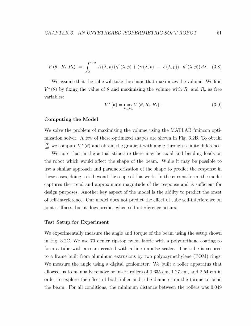
CHAPTER 3. AN UNTETHERED ISOPERIMETRIC SOFT ROBOT 61
V (θ, Rt, Rb) =
∫ Ltot
0
A (λ, p) (γ′ (λ, p) + (γ (λ, p) − c (λ, p)) · n′ (λ, p)) dλ. (3.8)
We assume that the tube will take the shape that maximizes the volume. We find
V ∗ (θ) by fixing the value of θ and maximizing the volume with Rt and Rb as free
variables:
V ∗ (θ) = maxRt,Rb
V (θ, Rt, Rb) . (3.9)
Computing the Model
We solve the problem of maximizing the volume using the MATLAB fmincon opti-
mization solver. A few of these optimized shapes are shown in Fig. 3.2B. To obtaindVdθ
we compute V ∗ (θ) and obtain the gradient with angle through a finite difference.
We note that in the actual structure there may be axial and bending loads on
the robot which would affect the shape of the beam. While it may be possible to
use a similar approach and parameterization of the shape to predict the response in
these cases, doing so is beyond the scope of this work. In the current form, the model
captures the trend and approximate magnitude of the response and is sufficient for
design purposes. Another key aspect of the model is the ability to predict the onset
of self-interference. Our model does not predict the effect of tube self-interference on
joint stiffness, but it does predict when self-interference occurs.
Test Setup for Experiment
We experimentally measure the angle and torque of the beam using the setup shown
in Fig. 3.2C. We use 70 denier ripstop nylon fabric with a polyurethane coating to
form a tube with a seam created with a line impulse sealer. The tube is secured
to a frame built from aluminum extrusions by two polyoxymethylene (POM) rings.
We measure the angle using a digital goniometer. We built a roller apparatus that
allowed us to manually remove or insert rollers of 0.635 cm, 1.27 cm, and 2.54 cm in
order to explore the effect of both roller and tube diameter on the torque to bend
the beam. For all conditions, the minimum distance between the rollers was 0.049
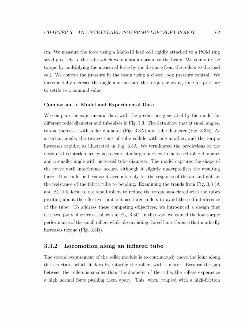
CHAPTER 3. AN UNTETHERED ISOPERIMETRIC SOFT ROBOT 62
cm. We measure the force using a Mark-10 load cell rigidly attached to a POM ring
sized precisely to the tube which we maintain normal to the beam. We compute the
torque by multiplying the measured force by the distance from the rollers to the load
cell. We control the pressure in the beam using a closed loop pressure control. We
incrementally increase the angle and measure the torque, allowing time for pressure
to settle to a nominal value.
Comparison of Model and Experimental Data
We compare the experimental data with the predictions generated by the model for
different roller diameter and tube sizes in Fig. 3.3. The data show that at small angles,
torque increases with roller diameter (Fig. 3.3A) and tube diameter (Fig. 3.3B). At
a certain angle, the two sections of tube collide with one another, and the torque
increases rapidly, as illustrated in Fig. 3.3A. We terminated the predictions at the
onset of this interference, which occurs at a larger angle with increased roller diameter
and a smaller angle with increased tube diameter. The model captures the shape of
the curve until interference occurs, although it slightly underpredicts the resulting
force. This could be because it accounts only for the response of the air and not for
the resistance of the fabric tube to bending. Examining the trends from Fig. 3.3 (A
and B), it is ideal to use small rollers to reduce the torque associated with the tubes
pivoting about the effective joint but use large rollers to avoid the self-interference
of the tube. To address these competing objectives, we introduced a design that
uses two pairs of rollers as shown in Fig. 3.3C. In this way, we gained the low-torque
performance of the small rollers while also avoiding the self-interference that markedly
increases torque (Fig. 3.3D).
3.3.2 Locomotion along an inflated tube
The second requirement of the roller module is to continuously move the joint along
the structure, which it does by rotating the rollers with a motor. Because the gap
between the rollers is smaller than the diameter of the tube, the rollers experience
a high normal force pushing them apart. This, when coupled with a high-friction

CHAPTER 3. AN UNTETHERED ISOPERIMETRIC SOFT ROBOT 63
BA
Self-Interference Begins
θ
dR=0.76 cmdR=1.14 cmdR=1.52 cm
Data ModeldT=4.60 cm
dT
0 50 100 1500
0.5
1
1.5
2
2.5
3
3.5
Torq
ue
(Nm
)
θ (°)
dT=7.32 cmdT=10.08 cm
Data Model
0 50 100 150θ (°)
0
1
2
3
4
Torq
ue
(Nm
)
0 50 100 1500
1
2
3
4
5To
rqu
e (N
m)
θ (°)
No RollerSingle RollerDouble Roller
Motor Gear
Cylindrical Rollers
C
In�ated Fabric Tube
dR
D
Figure 3.3: Analysis of the effective joint formed by rollers pinching a tube. (A) Therelationship between angle and torque with changing roller diameter (tube diameteris 7.32 cm). Model predictions are shown in solid lines and experimental data indashed lines. Torque at small angles increases with roller size, but interference, whichleads to a rapid increase in torque also begins at larger angles. (B) Increasing torquewith increasing tube diameters when the roller diameter is 1.14 cm. (C) The doubleroller configuration and the gear train that ensures all rollers move together from asingle motor input. (D) The torque required to bend a tube with no rollers, with asingle set of rollers, and with two sets of rollers as shown in (C) (roller diameters are0.64 cm separated by 6.35 cm). Reprinted from [13] with permission from AAAS.
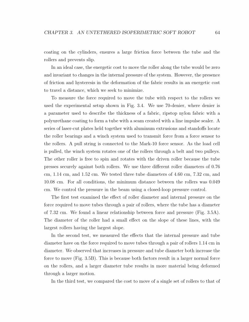
CHAPTER 3. AN UNTETHERED ISOPERIMETRIC SOFT ROBOT 64
coating on the cylinders, ensures a large friction force between the tube and the
rollers and prevents slip.
In an ideal case, the energetic cost to move the roller along the tube would be zero
and invariant to changes in the internal pressure of the system. However, the presence
of friction and hysteresis in the deformation of the fabric results in an energetic cost
to travel a distance, which we seek to minimize.
To measure the force required to move the tube with respect to the rollers we
used the experimental setup shown in Fig. 3.4. We use 70-denier, where denier is
a parameter used to describe the thickness of a fabric, ripstop nylon fabric with a
polyurethane coating to form a tube with a seam created with a line impulse sealer. A
series of laser-cut plates held together with aluminum extrusions and standoffs locate
the roller bearings and a winch system used to transmit force from a force sensor to
the rollers. A pull string is connected to the Mark-10 force sensor. As the load cell
is pulled, the winch system rotates one of the rollers through a belt and two pulleys.
The other roller is free to spin and rotates with the driven roller because the tube
presses securely against both rollers. We use three different roller diameters of 0.76
cm, 1.14 cm, and 1.52 cm. We tested three tube diameters of 4.60 cm, 7.32 cm, and
10.08 cm. For all conditions, the minimum distance between the rollers was 0.049
cm. We control the pressure in the beam using a closed-loop pressure control.
The first test examined the effect of roller diameter and internal pressure on the
force required to move tubes through a pair of rollers, where the tube has a diameter
of 7.32 cm. We found a linear relationship between force and pressure (Fig. 3.5A).
The diameter of the roller had a small effect on the slope of these lines, with the
largest rollers having the largest slope.
In the second test, we measured the effects that the internal pressure and tube
diameter have on the force required to move tubes through a pair of rollers 1.14 cm in
diameter. We observed that increases in pressure and tube diameter both increase the
force to move (Fig. 3.5B). This is because both factors result in a larger normal force
on the rollers, and a larger diameter tube results in more material being deformed
through a larger motion.
In the third test, we compared the cost to move of a single set of rollers to that of

CHAPTER 3. AN UNTETHERED ISOPERIMETRIC SOFT ROBOT 65
Figure 3.4: Test apparatus used to measure the force required to overcome frictionand move the tube through the rollers. An inflated tube was placed within the rollersand a force sensor was used to apply a torque on a shaft that was coupled to one ofthe rollers with a belt and pulleys. The entire length of the tube was slowly pulledthrough the rollers and the force required to move the rollers was averaged. Reprintedfrom [13] with permission from AAAS.
two pairs of rollers separated by a variable distance. In Fig. 3.5C, we show that the
cost to move for two pairs of rollers was less than twice that for one roller. Note that
we tested roller spacings less than a diameter of the tube because spacing greater
than a diameter is not effective at reducing joint torque and is thus not practical.
To characterize the relative magnitude of the forces required to move the tube
through the rollers, we compared the measured force with the maximum force that
could be exerted by the pressurized air, calculated as pressure times the cross-sectional
area of the tube. Across all of the data shown in Fig. 3.5, the forces required to move
the tube through the rollers had a peak of 14.6% and a mean of 8.78% of the maximum
force, indicating that the forces required to move the tube through the rollers are small
in comparison.
The above examination of the geometric effects on joint stiffness and the cost to
move enables us to make key design decisions. Using smaller rollers reduces the joint
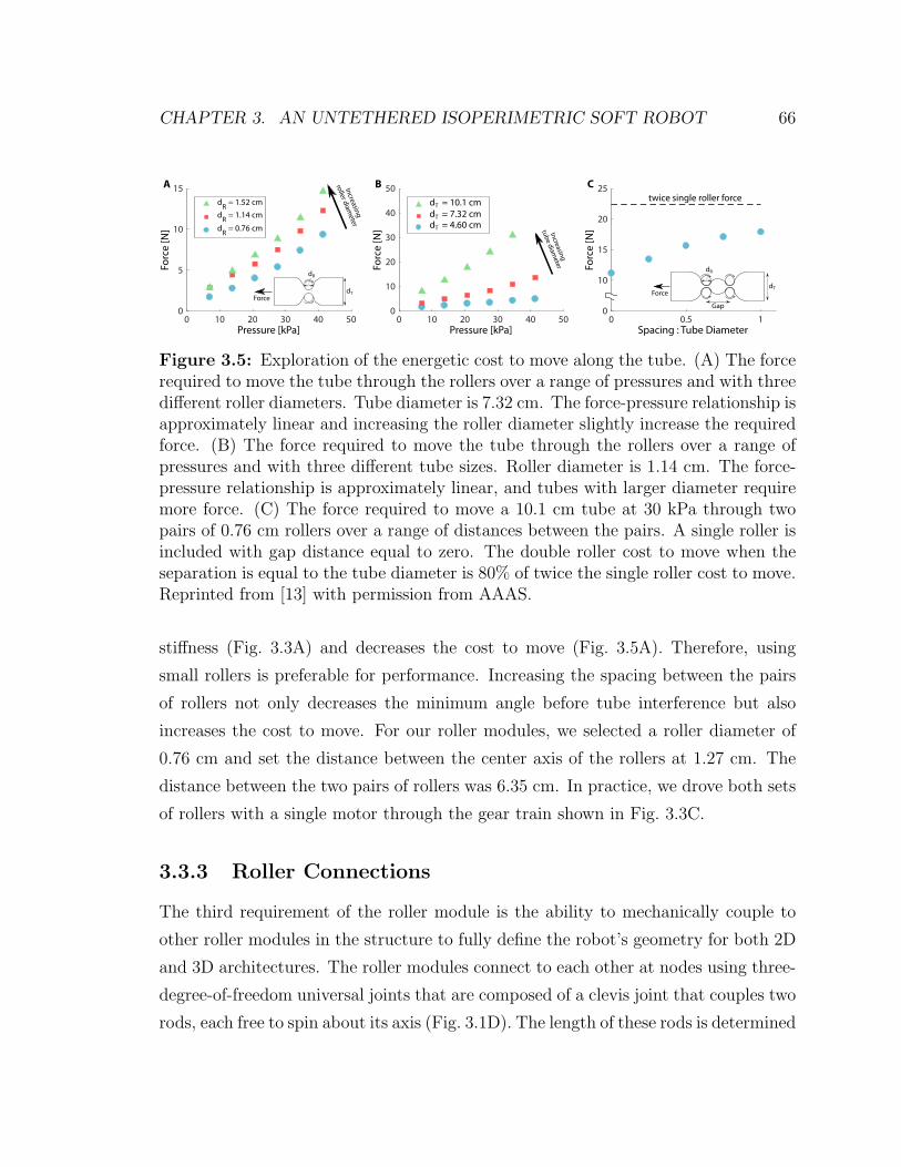
CHAPTER 3. AN UNTETHERED ISOPERIMETRIC SOFT ROBOT 66
0 0.5 1Spacing : Tube Diameter
0
10
15
20
25
Forc
e [N
]
0 10 20 30 40 50Pressure [kPa]
0
5
10
15
Forc
e [N
]
dR
= 1.52 cm
dR
= 1.14 cm
dR
= 0.76 cm
0 10 20 30 40 50Pressure [kPa]
0
10
20
30
40
50
Forc
e [N
]
dT = 10.1 cmdT = 7.32 cmdT = 4.60 cm
A BIncreasin
g
roller d
iameter
Increasin
g
tub
e diam
eter
dTForce
dR
Ctwice single roller force
dT
dR
Force
Gap
Figure 3.5: Exploration of the energetic cost to move along the tube. (A) The forcerequired to move the tube through the rollers over a range of pressures and with threedifferent roller diameters. Tube diameter is 7.32 cm. The force-pressure relationship isapproximately linear and increasing the roller diameter slightly increase the requiredforce. (B) The force required to move the tube through the rollers over a range ofpressures and with three different tube sizes. Roller diameter is 1.14 cm. The force-pressure relationship is approximately linear, and tubes with larger diameter requiremore force. (C) The force required to move a 10.1 cm tube at 30 kPa through twopairs of 0.76 cm rollers over a range of distances between the pairs. A single roller isincluded with gap distance equal to zero. The double roller cost to move when theseparation is equal to the tube diameter is 80% of twice the single roller cost to move.Reprinted from [13] with permission from AAAS.
stiffness (Fig. 3.3A) and decreases the cost to move (Fig. 3.5A). Therefore, using
small rollers is preferable for performance. Increasing the spacing between the pairs
of rollers not only decreases the minimum angle before tube interference but also
increases the cost to move. For our roller modules, we selected a roller diameter of
0.76 cm and set the distance between the center axis of the rollers at 1.27 cm. The
distance between the two pairs of rollers was 6.35 cm. In practice, we drove both sets
of rollers with a single motor through the gear train shown in Fig. 3.3C.
3.3.3 Roller Connections
The third requirement of the roller module is the ability to mechanically couple to
other roller modules in the structure to fully define the robot’s geometry for both 2D
and 3D architectures. The roller modules connect to each other at nodes using three-
degree-of-freedom universal joints that are composed of a clevis joint that couples two
rods, each free to spin about its axis (Fig. 3.1D). The length of these rods is determined

CHAPTER 3. AN UNTETHERED ISOPERIMETRIC SOFT ROBOT 67
by the size of the roller modules and the necessary minimum angle between these rods.
The mechanical design of the roller modules and the connections between them
must fully constrain the truss structure. Fully constrained means that any external
load induces a restoring force that seeks to return the structure back to an equilibrium
configuration. In the following section (Sec. 3.4) we present a kinematic analysis that
indicates that the structure is fully constrained if the connection point between a
roller module and its neighbor lies along the line that bisects the two segments of
tube joined by that roller. To achieve this constraint, we included two guide rings
as shown in Fig. 3.6. Each guide ring was attached to the body of the roller module
through arms that rotate about a pin joint concentric with the top roller in a pair
of rollers. In addition, we placed gear teeth on the arms supporting the guide rings
to couple the motion of the guide rings. We call these arms geared angle constraints
(Fig. 3.6). Together, the guide rings and the geared angle constraints ensured that
a central axis of the roller module bisects the two segments of tube, which, in turn,
ensured that the truss structure is fully constrained.
3.3.4 Construction
The inflatable tubes we used in our demonstration were constructed out of an outer
layer of heavy fabric and an inner air-tight bladder. We selected a commercially
available fabric with minimal stretch along the 45◦ bias. This fabric is a 200-denier
nylon fabric with an Oxford weave and a urethane coating (Seattle Fabrics Inc.).
The fabric was cut into a long rectangular piece and sewn together with a plain
seam and a straight stitch. A small hole was punched into the fabric for a pressure
line connector. The inner bladder was formed from a low-density polyethylene tube
(Hudson Exchange). This tube was cut to length, a hole was punched in its side for
the fitting, and the ends were heat-sealed. The inner bladder was inserted into the
fabric outer layer, and the ends of the outer layer were sewn shut with a straight
stitch. Last, a threaded through-wall pipe fitting was fastened in place where the
holes in each layer aligned. In practice, we inflated the tubes to about 40 kPa.
The housing of the roller module was created with laser-cut polyoxymethylene

CHAPTER 3. AN UNTETHERED ISOPERIMETRIC SOFT ROBOT 68
Geared Angle Constraints
Guide Rings
Node ConnectionBattery
Motor withEncoder
MotorGear
Idler Gear
Roller Gears
Roller withDycem
Microcontroller Motor Driver
Inner Plate(transparent)
Outer Plate(transparent )
Geared Angle Constraints (transparent)
Figure 3.6: Part callout of a roller module. Four parts in this figure are falselytransparent so that other parts can be shown. The outer plate on the right-handside and the two geared angle constraints on the right-hand side are transparent sothe transmission can be seen. The inner plate on the left-hand side is transparent sothe geared angle constraints can be seen. Reprinted from [13] with permission fromAAAS.
sheets. These pieces were fastened together with standoffs and corner brackets. The
housing contained holes to lightly press fit ball bearings that support the rotation of
the rollers and the gear train. The rollers were steel D-shafts wrapped in a nonslip
material (Dycem). External grooves were cut into the rollers, where retaining rings
were placed to locate the rollers with respect to the ball bearings. The custom gear
train had a speed multiplier of 3, which was selected for geometric convenience. Our
gear train was driven by a direct current motor with a planetary, reducing gear box
with a gear ratio of about 139:1 (ServoCity 638320). The motor was driven by a
Cytron MD10C motor driver in a drive-brake control method. The motor driver
was commanded by a Teensy 3.2 microcontroller, which used an nRF24l01+ radio
transceiver to receive position commands from an off-board laptop. The laptop was
not a necessary component because the position commands could be stored on the
microcontroller. The laptop provided a convenient user interface to send commands
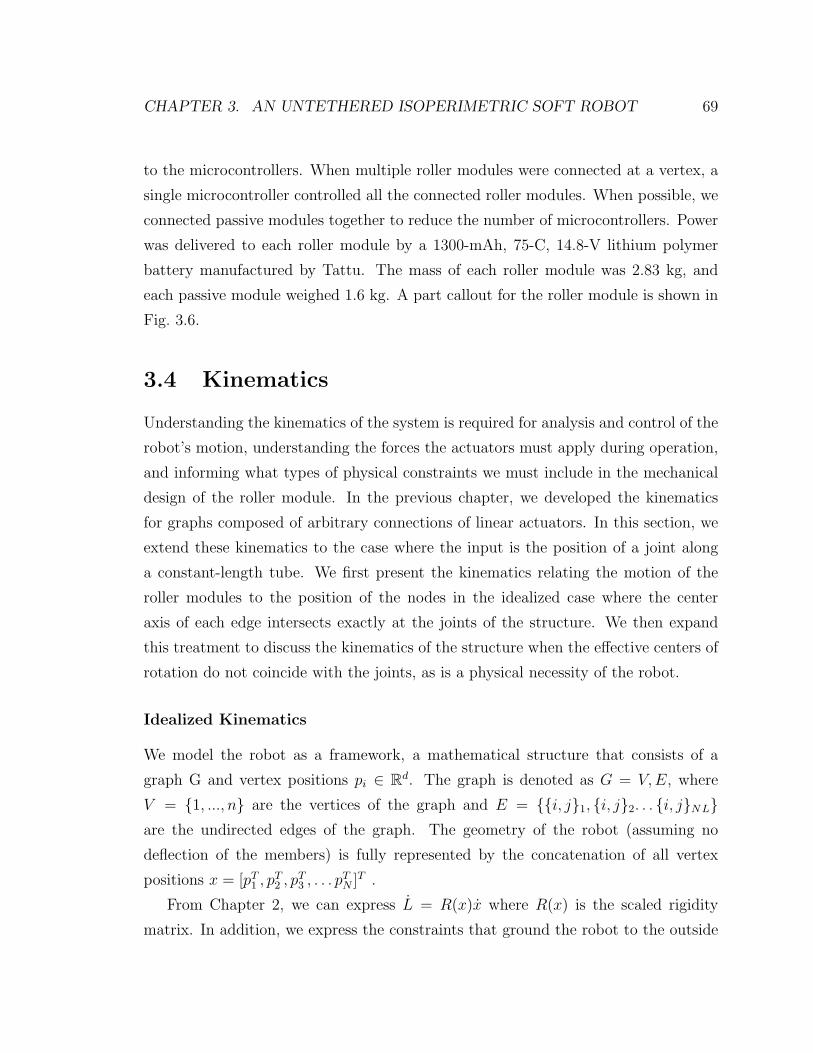
CHAPTER 3. AN UNTETHERED ISOPERIMETRIC SOFT ROBOT 69
to the microcontrollers. When multiple roller modules were connected at a vertex, a
single microcontroller controlled all the connected roller modules. When possible, we
connected passive modules together to reduce the number of microcontrollers. Power
was delivered to each roller module by a 1300-mAh, 75-C, 14.8-V lithium polymer
battery manufactured by Tattu. The mass of each roller module was 2.83 kg, and
each passive module weighed 1.6 kg. A part callout for the roller module is shown in
Fig. 3.6.
3.4 Kinematics
Understanding the kinematics of the system is required for analysis and control of the
robot’s motion, understanding the forces the actuators must apply during operation,
and informing what types of physical constraints we must include in the mechanical
design of the roller module. In the previous chapter, we developed the kinematics
for graphs composed of arbitrary connections of linear actuators. In this section, we
extend these kinematics to the case where the input is the position of a joint along
a constant-length tube. We first present the kinematics relating the motion of the
roller modules to the position of the nodes in the idealized case where the center
axis of each edge intersects exactly at the joints of the structure. We then expand
this treatment to discuss the kinematics of the structure when the effective centers of
rotation do not coincide with the joints, as is a physical necessity of the robot.
Idealized Kinematics
We model the robot as a framework, a mathematical structure that consists of a
graph G and vertex positions pi ∈ Rd. The graph is denoted as G = V,E, where
V = {1, ..., n} are the vertices of the graph and E = {{i, j}1, {i, j}2. . . {i, j}NL}are the undirected edges of the graph. The geometry of the robot (assuming no
deflection of the members) is fully represented by the concatenation of all vertex
positions x = [pT1 , pT2 , p
T3 , . . . p
TN ]T .
From Chapter 2, we can express L = R(x)x where R(x) is the scaled rigidity
matrix. In addition, we express the constraints that ground the robot to the outside
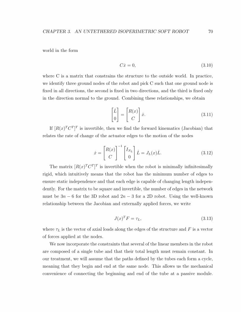
CHAPTER 3. AN UNTETHERED ISOPERIMETRIC SOFT ROBOT 70
world in the form
Cx = 0, (3.10)
where C is a matrix that constrains the structure to the outside world. In practice,
we identify three ground nodes of the robot and pick C such that one ground node is
fixed in all directions, the second is fixed in two directions, and the third is fixed only
in the direction normal to the ground. Combining these relationships, we obtain[L
0
]=
[R(x)
C
]x. (3.11)
If [R(x)TCT ]T is invertible, then we find the forward kinematics (Jacobian) that
relates the rate of change of the actuator edges to the motion of the nodes
x =
[R(x)
C
]−1 [INL
0
]L = JL(x)L. (3.12)
The matrix [R(x)TCT ]T is invertible when the robot is minimally infinitesimally
rigid, which intuitively means that the robot has the minimum number of edges to
ensure static independence and that each edge is capable of changing length indepen-
dently. For the matrix to be square and invertible, the number of edges in the network
must be 3n − 6 for the 3D robot and 2n − 3 for a 2D robot. Using the well-known
relationship between the Jacobian and externally applied forces, we write
J(x)TF = τL, (3.13)
where τL is the vector of axial loads along the edges of the structure and F is a vector
of forces applied at the nodes.
We now incorporate the constraints that several of the linear members in the robot
are composed of a single tube and that their total length must remain constant. In
our treatment, we will assume that the paths defined by the tubes each form a cycle,
meaning that they begin and end at the same node. This allows us the mechanical
convenience of connecting the beginning and end of the tube at a passive module.

CHAPTER 3. AN UNTETHERED ISOPERIMETRIC SOFT ROBOT 71
Including paths that start and end at different nodes requires only minor modification.
The path of the tube or tubes through the robot is defined by an ordered pair of nodes,
where each stop at a node corresponds with a roller module, which we number 1 to
Nroller. We represent these paths as a matrix Ball(G) ∈ RNroller,NL . Each column of
Ball corresponds to one edge of the graph and has exactly two nonzero entries: a 1
in the row corresponding to the tail node of the directed edge and a 1 at the row
corresponding to the head of the directed edge. This matrix allows us to relate the
velocity of the rollers to the rate of change of the edge lengths
L = BTallrrollerθ, (3.14)
where θ corresponds to the position of each of the motor of each roller. To relate the
motion of the rollers directly to the motion of the nodes, we combine Eqs. 3.12 and
3.14 to obtain
x =
[R(x)
C
]−1 [BTall
0
]rrollerθ = Jθ(x)θ. (3.15)
The Jacobian Jθ(x) relates the motor motions to node motions, which also allows
us to quantify the torque required from the motors to hold a particular configuration
as τroller = Jθ(x)TF .
We note that the sum of all of the edge lengths of the structure is obtained as
1TL. We can confirm that the total length of the shared member is unchanged for
any combination of roller velocity inputs by showing that 1TBT = 0, which is a result
of the construction of the B matrix, as we have ensured that each column sums to 0.
If each tube in the robot is a single continuous loop with no end, all the roller
modules could run at the same speed and the tube would move continuously, while
all the nodes remain stationary, as indicated by the fact that BT1 = 0. In practice,
we do not include a motor at the node that makes up the first and last connection for
each tube, which corresponds to removing the elements of θ and columns of B that
correspond to the first and last node of each tube in the robot.

CHAPTER 3. AN UNTETHERED ISOPERIMETRIC SOFT ROBOT 72
A
B
C E
D
Figure 3.7: An illustration of the three points at each roller module that are usedto represent the state of the robot. Point A is the connection between two rollermodules. Points B and D are the center points of the rollers. Points C and E arethe opposite ends of the respective edges. Reprinted from [13] with permission fromAAAS.
3.4.1 Kinematics in the presence of offsets
In practice, it is not possible for the edges to intersect at the nodes due to the large
size of the tubes and the double-roller design of each roller module (Fig. 3.6). In the
presence of these offsets, we represent the kinematic state of each roller module as
the position of three points. These points are illustrated in Fig. 3.7 and are the point
where two roller modules connect (denoted point A) and the point at the center of
each pair of rollers in plane with the inflated tube (points B and D). We denote the
point at the opposite end of each tube segment from points B and D as points C and
E, respectively. We want to impose sufficient constraints in the physical design of the
roller module so as to fully constrain the kinematic state of all roller modules (points
A, B, and D for each module). For a robot in 3D, each new point introduced into
the kinematic state introduces three new degrees of freedom. For each roller module,
we must remove six degrees of freedom. We chose to include two guide rings that are

CHAPTER 3. AN UNTETHERED ISOPERIMETRIC SOFT ROBOT 73
geared together such that they, along with the mechanical construction of the roller
module, enable the following mathematical constraints:
• All edges in the triangle formed by points A, B, and D are constant length.
The resulting forces are provided by the physical structure of the roller module.
This imposes three constraints that are of the same form as the constraints in
(1). We take the derivative of these constraints and rearrange them into the
matrix Rnode(x).
• A constraint that the angle CBD is equal to the angle EDB.This constraint is
provided by gear teeth that are included onto the arms of the angle constraint
shown in Fig. 3.6. This imposes one constraint, which is expressed
(xd − xb)T (xc − xb)‖(xd − xb)‖‖(xc − xb)‖
=(xe − xc)T (xb − xc)‖(xe − xc)‖‖(xb − xc)‖
(3.16)
We take the derivative of this constraint for each roller module in the network
and put the result into the matrix Rbisect(x).
• A constraint that point A remains in the plane defined by points B, C, and D
and the plane defined by points B, C, and E. This constraint requires coupling
between the edges and the rollers in a direction normal to both edges. This
imposes two constraints, which are enforced by the guide rings. This constraint
is only necessary when the robot is in 3D. These constraints are expressed
(xa − xb)T ((xc − xb)× (xd − xb))‖(xd − xb))‖‖(xc − xb)× (xd − xb)‖
= 0 (3.17)
and(xa − xc)T ((xb − xc)× (xe − xc))‖(xe − xc))‖‖(xb − xc)× (xe − xc)‖
= 0 (3.18)
We again take the derivative of each of these constraints in the current config-
uration and put the result into the matrix Rplanar(x).
We combine these results to form the following result
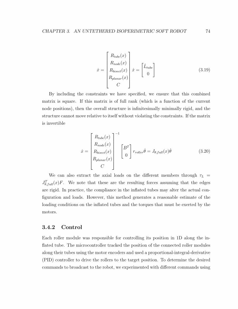
CHAPTER 3. AN UNTETHERED ISOPERIMETRIC SOFT ROBOT 74
x =
Rtube(x)
Rnode(x)
Rbisect(x)
Rplanar(x)
C
x =
[Ltube
0
](3.19)
By including the constraints we have specified, we ensure that this combined
matrix is square. If this matrix is of full rank (which is a function of the current
node positions), then the overall structure is infinitesimally minimally rigid, and the
structure cannot move relative to itself without violating the constraints. If the matrix
is invertible
x =
Rtube(x)
Rnode(x)
Rbisect(x)
Rplanar(x)
C
−1
[BT
0
]rrollerθ = Jθ,full(x)θ (3.20)
We can also extract the axial loads on the different members through τL =
JTθ,full(x)F . We note that these are the resulting forces assuming that the edges
are rigid. In practice, the compliance in the inflated tubes may alter the actual con-
figuration and loads. However, this method generates a reasonable estimate of the
loading conditions on the inflated tubes and the torques that must be exerted by the
motors.
3.4.2 Control
Each roller module was responsible for controlling its position in 1D along the in-
flated tube. The microcontroller tracked the position of the connected roller modules
along their tubes using the motor encoders and used a proportional-integral-derivative
(PID) controller to drive the rollers to the target position. To determine the desired
commands to broadcast to the robot, we experimented with different commands using
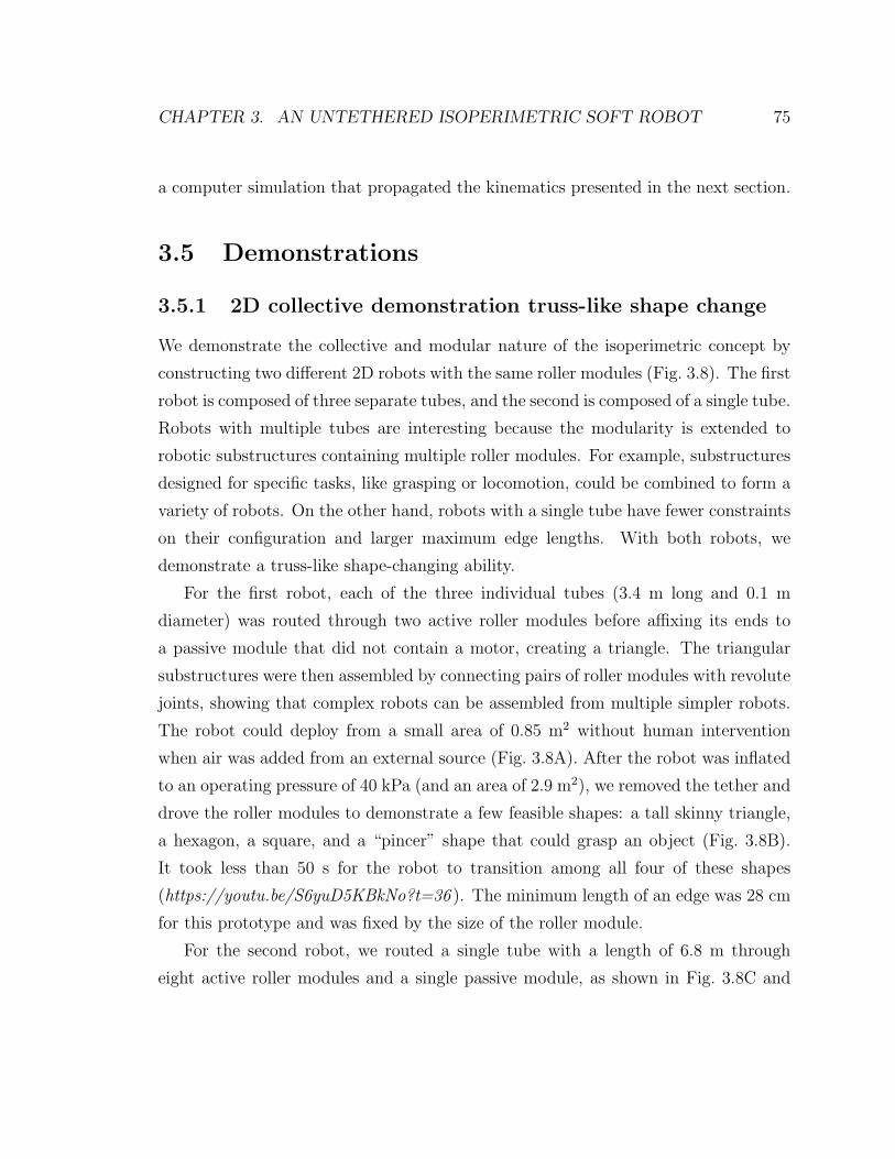
CHAPTER 3. AN UNTETHERED ISOPERIMETRIC SOFT ROBOT 75
a computer simulation that propagated the kinematics presented in the next section.
3.5 Demonstrations
3.5.1 2D collective demonstration truss-like shape change
We demonstrate the collective and modular nature of the isoperimetric concept by
constructing two different 2D robots with the same roller modules (Fig. 3.8). The first
robot is composed of three separate tubes, and the second is composed of a single tube.
Robots with multiple tubes are interesting because the modularity is extended to
robotic substructures containing multiple roller modules. For example, substructures
designed for specific tasks, like grasping or locomotion, could be combined to form a
variety of robots. On the other hand, robots with a single tube have fewer constraints
on their configuration and larger maximum edge lengths. With both robots, we
demonstrate a truss-like shape-changing ability.
For the first robot, each of the three individual tubes (3.4 m long and 0.1 m
diameter) was routed through two active roller modules before affixing its ends to
a passive module that did not contain a motor, creating a triangle. The triangular
substructures were then assembled by connecting pairs of roller modules with revolute
joints, showing that complex robots can be assembled from multiple simpler robots.
The robot could deploy from a small area of 0.85 m2 without human intervention
when air was added from an external source (Fig. 3.8A). After the robot was inflated
to an operating pressure of 40 kPa (and an area of 2.9 m2), we removed the tether and
drove the roller modules to demonstrate a few feasible shapes: a tall skinny triangle,
a hexagon, a square, and a “pincer” shape that could grasp an object (Fig. 3.8B).
It took less than 50 s for the robot to transition among all four of these shapes
(https://youtu.be/S6yuD5KBkNo?t=36 ). The minimum length of an edge was 28 cm
for this prototype and was fixed by the size of the roller module.
For the second robot, we routed a single tube with a length of 6.8 m through
eight active roller modules and a single passive module, as shown in Fig. 3.8C and
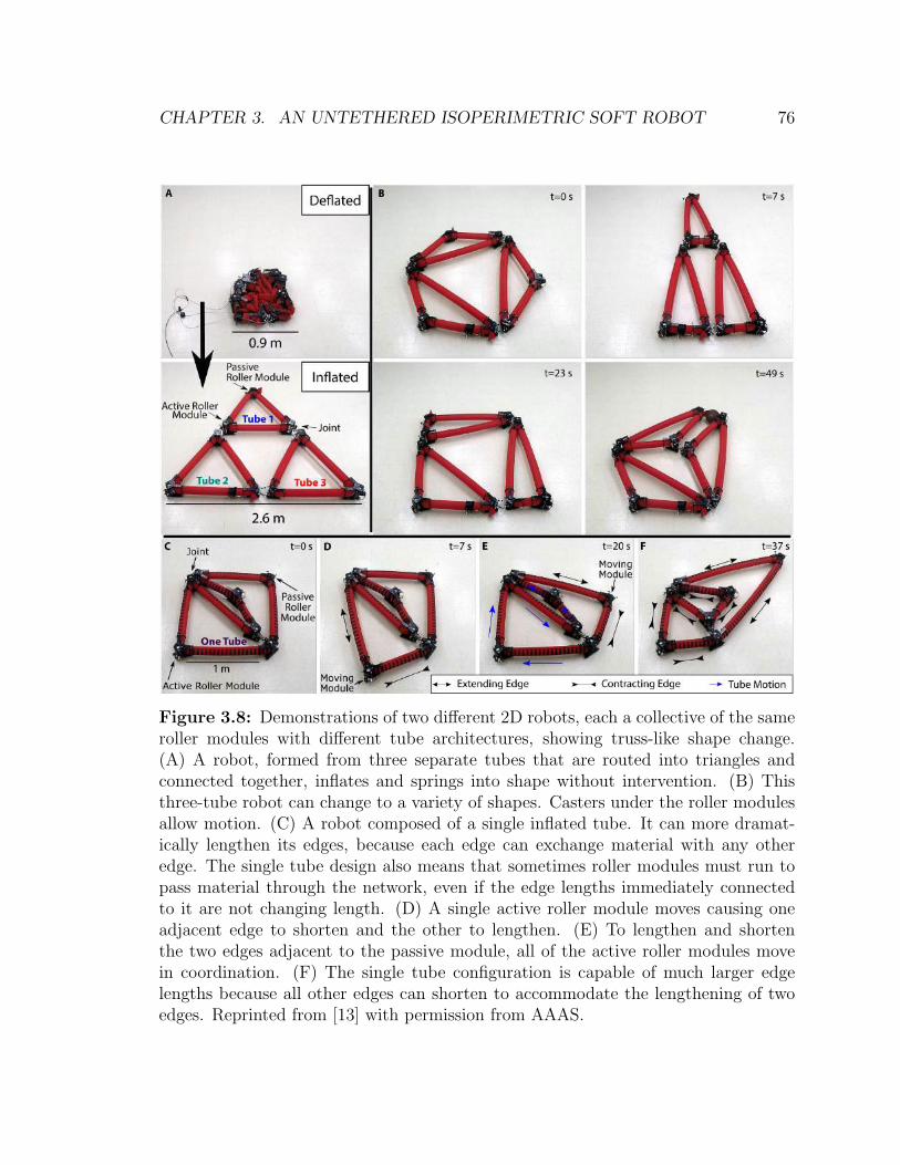
CHAPTER 3. AN UNTETHERED ISOPERIMETRIC SOFT ROBOT 76
Figure 3.8: Demonstrations of two different 2D robots, each a collective of the sameroller modules with different tube architectures, showing truss-like shape change.(A) A robot, formed from three separate tubes that are routed into triangles andconnected together, inflates and springs into shape without intervention. (B) Thisthree-tube robot can change to a variety of shapes. Casters under the roller modulesallow motion. (C) A robot composed of a single inflated tube. It can more dramat-ically lengthen its edges, because each edge can exchange material with any otheredge. The single tube design also means that sometimes roller modules must run topass material through the network, even if the edge lengths immediately connectedto it are not changing length. (D) A single active roller module moves causing oneadjacent edge to shorten and the other to lengthen. (E) To lengthen and shortenthe two edges adjacent to the passive module, all of the active roller modules movein coordination. (F) The single tube configuration is capable of much larger edgelengths because all other edges can shorten to accommodate the lengthening of twoedges. Reprinted from [13] with permission from AAAS.
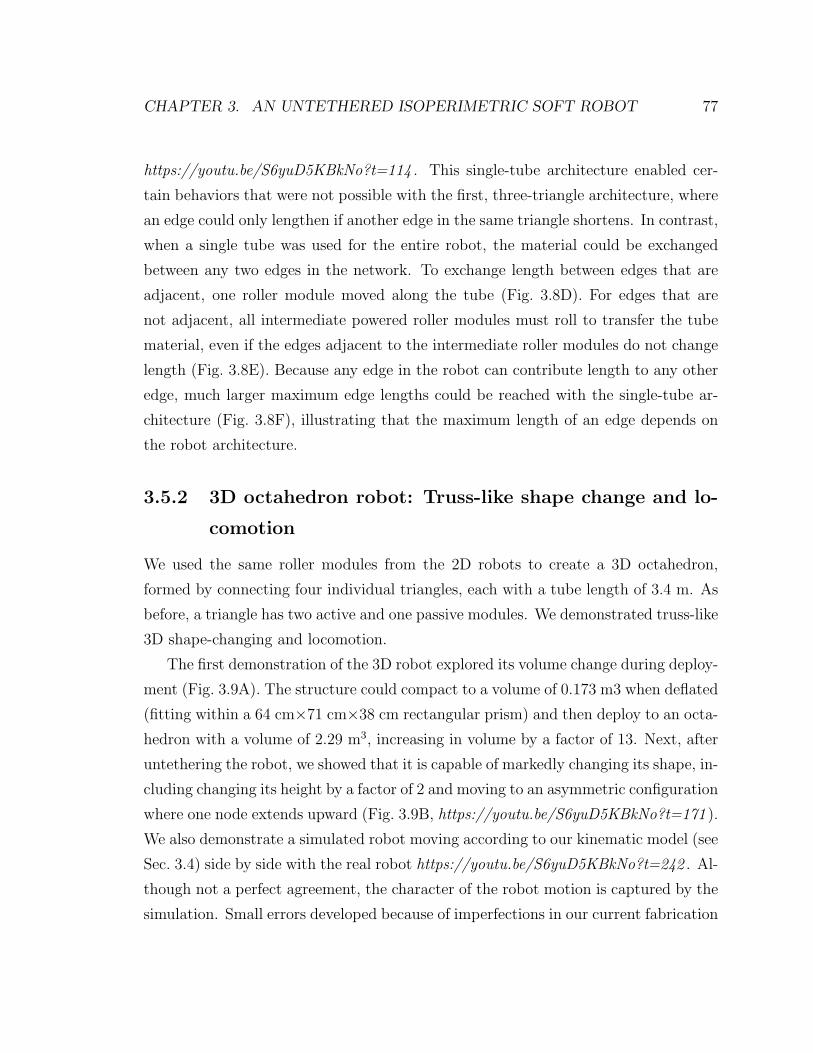
CHAPTER 3. AN UNTETHERED ISOPERIMETRIC SOFT ROBOT 77
https://youtu.be/S6yuD5KBkNo?t=114 . This single-tube architecture enabled cer-
tain behaviors that were not possible with the first, three-triangle architecture, where
an edge could only lengthen if another edge in the same triangle shortens. In contrast,
when a single tube was used for the entire robot, the material could be exchanged
between any two edges in the network. To exchange length between edges that are
adjacent, one roller module moved along the tube (Fig. 3.8D). For edges that are
not adjacent, all intermediate powered roller modules must roll to transfer the tube
material, even if the edges adjacent to the intermediate roller modules do not change
length (Fig. 3.8E). Because any edge in the robot can contribute length to any other
edge, much larger maximum edge lengths could be reached with the single-tube ar-
chitecture (Fig. 3.8F), illustrating that the maximum length of an edge depends on
the robot architecture.
3.5.2 3D octahedron robot: Truss-like shape change and lo-
comotion
We used the same roller modules from the 2D robots to create a 3D octahedron,
formed by connecting four individual triangles, each with a tube length of 3.4 m. As
before, a triangle has two active and one passive modules. We demonstrated truss-like
3D shape-changing and locomotion.
The first demonstration of the 3D robot explored its volume change during deploy-
ment (Fig. 3.9A). The structure could compact to a volume of 0.173 m3 when deflated
(fitting within a 64 cm×71 cm×38 cm rectangular prism) and then deploy to an octa-
hedron with a volume of 2.29 m3, increasing in volume by a factor of 13. Next, after
untethering the robot, we showed that it is capable of markedly changing its shape, in-
cluding changing its height by a factor of 2 and moving to an asymmetric configuration
where one node extends upward (Fig. 3.9B, https://youtu.be/S6yuD5KBkNo?t=171 ).
We also demonstrate a simulated robot moving according to our kinematic model (see
Sec. 3.4) side by side with the real robot https://youtu.be/S6yuD5KBkNo?t=242 . Al-
though not a perfect agreement, the character of the robot motion is captured by the
simulation. Small errors developed because of imperfections in our current fabrication
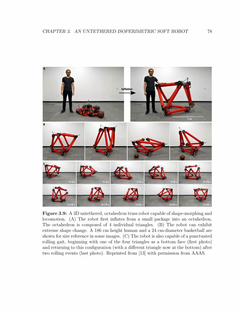
CHAPTER 3. AN UNTETHERED ISOPERIMETRIC SOFT ROBOT 78
Figure 3.9: A 3D untethered, octahedron truss robot capable of shape-morphing andlocomotion. (A) The robot first inflates from a small package into an octahedron.The octahedron is composed of 4 individual triangles. (B) The robot can exhibitextreme shape change. A 186 cm height human and a 24 cm-diameter basketball areshown for size reference in some images. (C) The robot is also capable of a punctuatedrolling gait, beginning with one of the four triangles as a bottom face (first photo)and returning to this configuration (with a different triangle now at the bottom) aftertwo rolling events (last photo). Reprinted from [13] with permission from AAAS.
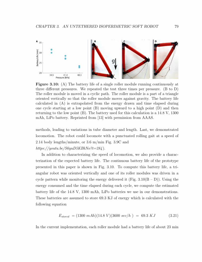
CHAPTER 3. AN UNTETHERED ISOPERIMETRIC SOFT ROBOT 79
Figure 3.10: (A) The battery life of a single roller module running continuously atthree different pressures. We repeated the test three times per pressure. (B to D)The roller module is moved in a cyclic path. The roller module is a part of a triangleoriented vertically so that the roller module moves against gravity. The battery lifecalculated in (A) is extrapolated from the energy drawn and time elapsed duringone cycle starting at a low point (B) moving upward to a high point (D) and thenreturning to the low point (B). The battery used for this calculation is a 14.8 V, 1300mAh, LiPo battery. Reprinted from [13] with permission from AAAS.
methods, leading to variations in tube diameter and length. Last, we demonstrated
locomotion. The robot could locomote with a punctuated rolling gait at a speed of
2.14 body lengths/minute, or 3.6 m/min Fig. 3.9C and
https://youtu.be/S6yuD5KBkNo?t=284 ).
In addition to characterizing the speed of locomotion, we also provide a charac-
terization of the expected battery life. The continuous battery life of the prototype
presented in this paper is shown in Fig. 3.10. To compute this battery life, a tri-
angular robot was oriented vertically and one of its roller modules was driven in a
cycle pattern while monitoring the energy delivered it (Fig. 3.10(B – D)). Using the
energy consumed and the time elapsed during each cycle, we compute the estimated
battery life of the 14.8 V, 1300 mAh, LiPo batteries we use in our demonstrations.
These batteries are assumed to store 69.3 KJ of energy which is calculated with the
following equation
Estored = (1300 mAh)(14.8 V )(3600 sec/h ) = 69.3 KJ (3.21)
In the current implementation, each roller module had a battery life of about 23 min
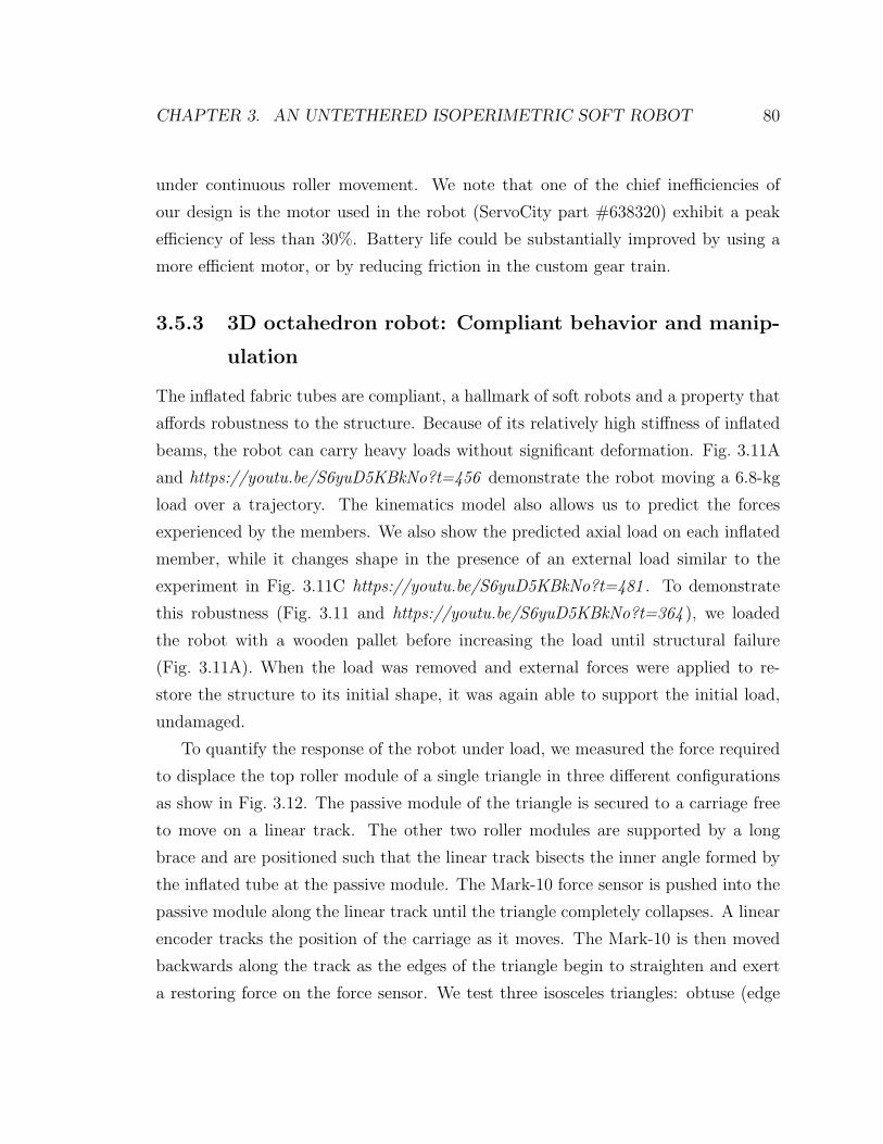
CHAPTER 3. AN UNTETHERED ISOPERIMETRIC SOFT ROBOT 80
under continuous roller movement. We note that one of the chief inefficiencies of
our design is the motor used in the robot (ServoCity part #638320) exhibit a peak
efficiency of less than 30%. Battery life could be substantially improved by using a
more efficient motor, or by reducing friction in the custom gear train.
3.5.3 3D octahedron robot: Compliant behavior and manip-
ulation
The inflated fabric tubes are compliant, a hallmark of soft robots and a property that
affords robustness to the structure. Because of its relatively high stiffness of inflated
beams, the robot can carry heavy loads without significant deformation. Fig. 3.11A
and https://youtu.be/S6yuD5KBkNo?t=456 demonstrate the robot moving a 6.8-kg
load over a trajectory. The kinematics model also allows us to predict the forces
experienced by the members. We also show the predicted axial load on each inflated
member, while it changes shape in the presence of an external load similar to the
experiment in Fig. 3.11C https://youtu.be/S6yuD5KBkNo?t=481 . To demonstrate
this robustness (Fig. 3.11 and https://youtu.be/S6yuD5KBkNo?t=364 ), we loaded
the robot with a wooden pallet before increasing the load until structural failure
(Fig. 3.11A). When the load was removed and external forces were applied to re-
store the structure to its initial shape, it was again able to support the initial load,
undamaged.
To quantify the response of the robot under load, we measured the force required
to displace the top roller module of a single triangle in three different configurations
as show in Fig. 3.12. The passive module of the triangle is secured to a carriage free
to move on a linear track. The other two roller modules are supported by a long
brace and are positioned such that the linear track bisects the inner angle formed by
the inflated tube at the passive module. The Mark-10 force sensor is pushed into the
passive module along the linear track until the triangle completely collapses. A linear
encoder tracks the position of the carriage as it moves. The Mark-10 is then moved
backwards along the track as the edges of the triangle begin to straighten and exert
a restoring force on the force sensor. We test three isosceles triangles: obtuse (edge

CHAPTER 3. AN UNTETHERED ISOPERIMETRIC SOFT ROBOT 81
Figure 3.11: Demonstration and characterization of the robot’s compliant behavior.(A) Overloading the robot causes the robot to collapse. After being restored to itsinitial configuration, the robot is again able to support the initial load. (B) Theload displacement behavior of a single triangle in three different configurations. Inall cases, there is a moderate initial stiffness until a critical load is reached and thebeam buckles, at which point the force required to maintain a given level of deflectionis much lower than the peak value, demonstrating a mechanical-fuse-type behavior ofthe robot. (C) The robot moves a 6.8 kg load over a trajectory. Reprinted from [13]with permission from AAAS.
lengths of 89 cm, 89 cm, and 128 cm, Fig. 3.12B), equilateral (edge lengths of 102 cm,
Fig. 3.12C), and acute (edge lengths of 121 cm, 121 cm, and 64 cm, Fig. 3.12D). The
initial pressure is set using a closed-loop pressure control and was set at 41.4 kPa.
At the beginning of the test, a valve is closed such that the tests are performed with
a fixed mass of air within the tube. The results are shown in Fig. 3.12A. When an
external load was applied to a node of the truss structure, there was a relatively high
initial stiffness until the load causes one of the beams to buckle, at which point the
force exerted at the node markedly decreases, approaching a zero-stiffness regime.
This behavior is like a mechanical fuse: During normal operation, the structure is
relatively stiff, allowing functionality; yet, beyond some threshold force, it buckles,
limiting damage to itself or the environment. The exact level of the threshold force
could be tuned via control of the robot configuration, leveraging existing work on the
mechanics of inflated beams [94,95,96].
Different recovery strategies can be invoked after an inflated beam buckles. Oc-
casionally, the beam will recover on its own when the load is removed. This is due
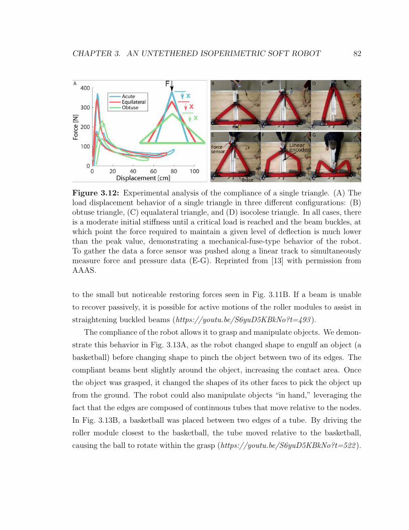
CHAPTER 3. AN UNTETHERED ISOPERIMETRIC SOFT ROBOT 82
Figure 3.12: Experimental analysis of the compliance of a single triangle. (A) Theload displacement behavior of a single triangle in three different configurations: (B)obtuse triangle, (C) equalateral triangle, and (D) isocolese triangle. In all cases, thereis a moderate initial stiffness until a critical load is reached and the beam buckles, atwhich point the force required to maintain a given level of deflection is much lowerthan the peak value, demonstrating a mechanical-fuse-type behavior of the robot.To gather the data a force sensor was pushed along a linear track to simultaneouslymeasure force and pressure data (E-G). Reprinted from [13] with permission fromAAAS.
to the small but noticeable restoring forces seen in Fig. 3.11B. If a beam is unable
to recover passively, it is possible for active motions of the roller modules to assist in
straightening buckled beams (https://youtu.be/S6yuD5KBkNo?t=493 ).
The compliance of the robot allows it to grasp and manipulate objects. We demon-
strate this behavior in Fig. 3.13A, as the robot changed shape to engulf an object (a
basketball) before changing shape to pinch the object between two of its edges. The
compliant beams bent slightly around the object, increasing the contact area. Once
the object was grasped, it changed the shapes of its other faces to pick the object up
from the ground. The robot could also manipulate objects “in hand,” leveraging the
fact that the edges are composed of continuous tubes that move relative to the nodes.
In Fig. 3.13B, a basketball was placed between two edges of a tube. By driving the
roller module closest to the basketball, the tube moved relative to the basketball,
causing the ball to rotate within the grasp (https://youtu.be/S6yuD5KBkNo?t=522 ).
CHAPTER 3. AN UNTETHERED ISOPERIMETRIC SOFT ROBOT 83
Figure 3.13: Demonstration of the robot’s ability to use its inherent compliance tomanipulate and interact with objects. (A) The robot grasps a basketball (diameter of24 cm, mass of 580 g) by first engulfing it, and then pinching it between two compliantedges. The robot then change shape to lift the basketball into the air. (B) With thebasketball secured between two edges, motion of the roller module closest to thebasketball cause the basketball to spin. A coordinate frame has been added to allowvisualization of how the orientation of the basketball changes. The basketball rotatesapproximately 135 degrees between the second and third configurations. Reprintedfrom [13] with permission from AAAS.
3.6 Tradeoffs: Workspace, efficiency, and speed
We now discuss the tradeoffs inherent in the isoperimetric robot design and compare
this robot to truss and pneumatically actuated robots. In the first set of comparisons,
we examined the effect of kinematic differences between an isoperimetric robot and
a conventional truss robot on their respective workspace. Next, we analyzed how
these kinematic differences affect efficiency and speed of movements. In the last set
of comparisons, we examined the effect of the power source—electric motors for the
isoperimetric robots and microcompressors for pneumatically actuated robots—on
efficiency and speed.
3.6.1 Effects of kinematic differences on workspace
We qualitatively then quantitatively compare the workspace of a conventional truss
robot with that of our robot. Qualitatively, in the conventional truss robot, each

CHAPTER 3. AN UNTETHERED ISOPERIMETRIC SOFT ROBOT 84
edge is a linear actuator with a fixed amount of material that is locally reconfigured
to change the edge length. In our robot, each edge can exchange material with
other edges to change length. This reallocation of material is conceptually similar to
changing the shape of a fixed mass of clay: The shape can change markedly, but the
total amount of material must remain the same. In many cases, our concept allows
for larger extremes in the length of an individual edge than does a conventional truss
robot. However, it also necessitates coupling for changes in the length of edges that are
part of the same tube. Each individual tube in the architecture represents another
constraint on the achievable configuration space and a potential reduction of the
workspace. As a result, an isoperimetric robot will have fewer degrees of freedom than
a robot composed of linear actuators with the same graphical structure. Therefore,
some motions that are possible for a conventional truss robot are impossible for our
robots. The octahedron robot, for example, cannot reduce its total edge length to
become a smaller regular octahedron, although its enclosed volume can substantially
change. The mathematical form of these constraints is discussed in Sec. 3.4.
Next, we quantitatively compare the reachable workspaces of the top node of
three different 2D triangular robot architectures: an isoperimetric robot with two
active roller modules, a conventional truss robot with a linear actuator on each edge,
and a conventional truss robot with linear actuators on two edges and supported
by two pinned nodes (Fig. 3.14 and https://youtu.be/S6yuD5KBkNo?t=582 ). The
workspace of our robot completely covers the workspace of the robot composed of
three linear actuators, which, in turn, completely covers the workspace of the robot
composed of two linear actuators. The workspace of our robot is 3.4 times larger than
the workspace of the robot composed of three linear actuators and 6.8 times larger
than the workspace of the robot composed of two linear actuators. These results
indicate that, in some cases, the isoperimetric architecture may increase a robot’s
workspace. We also compare the manipulability index µ for node 2 throughout the
two robots’ respective workspaces (Fig. 3.14C,D) [97]. The manipulability index is
the volume of the manipulability ellipsoid that represents the node velocity resulting
from normalized actuator inputs. Larger manipulability indices correspond to larger
end effector motions given fixed actuator inputs. The manipulability index is higher
CHAPTER 3. AN UNTETHERED ISOPERIMETRIC SOFT ROBOT 85
for the isoperimetric robot than the robot with two linear actuators across the shared
workspace, indicating the possibility of faster motions, but with the corresponding
result that higher actuator torques are required to resist external loads. For the robot
with three linear actuators, the robot has redundancy to the task of positioning node
2, which we exploit to maximize the manipulability. Even so, the isoperimetric robot
has higher manipulability in a portion of the shared workspace.
3.6.2 Effects of kinematic differences on efficiency and speed
We first qualitatively, then quantitatively, compare how the kinematics of an isoperi-
metric robot and a truss robot affect the efficiency and speed of motion. Qualitatively,
the added constraints on the isoperimetric robot mean that certain motions require
much more energy or must be performed more slowly than others—a factor that
should be considered when planning movements. This can be explained as follows:
Unlike in a truss robot, the number of actuators (for our robot, roller modules) needed
to change the robot’s configuration is not necessarily equal to the number of edges
that are changing in length. For example, exchanging length between the two edges
adjacent to the same active roller module (edges 1 and 2 in Fig. 3.15A) requires only
the energy to operate one roller module. However, exchanging length between edges
separated by multiple active roller modules (edges 1 and 3) requires multiple roller
modules to drive. These effects are exacerbated if a single tube covers more than
three edges in a triangle, as illustrated in Fig. 3.8(D and E). The coupling between
edge length changes and the routing of the tube also affects the rate of change of
different edge lengths. For the robot in Fig. 3.15A, edge 2 can lengthen at twice the
maximum speed of the rollers and hence twice the maximum speed of edges 1 and 3
due to the fact that it has active rollers on both ends. However, it can only extend at
maximum speed if both edges 1 and 3 are contracting at the maximum speed. These
dependencies illustrate that the energy required to perform a given motion and the
speed at which edge lengths can change depend on the architecture of the graph, not
just the parameters of the actuators as in a truss robot composed of linear actuators.
In simulation we compare the efficiency and speed of an idealized isoperimetric
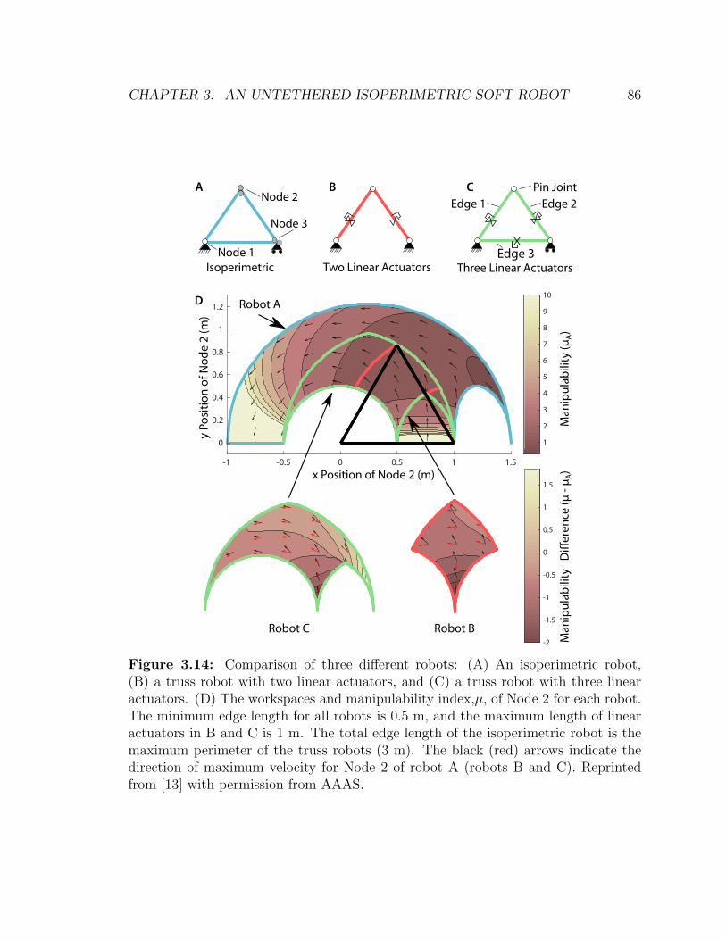
CHAPTER 3. AN UNTETHERED ISOPERIMETRIC SOFT ROBOT 86
0.2
0.4
0.6
0.8
-1 -0.5 0 0.5 1 1.5
0
0.2
0.4
0.6
0.8
1
1.2
1
2
3
4
5
6
7
8
9
10
Node 2
Node 3
IsoperimetricNode 1
A
y P
osi
tio
n o
f N
od
e 2
(m)
x Position of Node 2 (m)
D
Robot C Robot B
Man
ipu
lab
ility
(μA)
Robot A
Man
ipu
lab
ility
D
iffe
ren
ce (μ
- μ
A)
-0.5 0 0.5 1 1.5
-2
-1.5
-1
-0.5
0
0.5
1
1.5
Two Linear Actuators
B Pin Joint
Three Linear Actuators
C
Edge 1 Edge 2
Edge 3
Figure 3.14: Comparison of three different robots: (A) An isoperimetric robot,(B) a truss robot with two linear actuators, and (C) a truss robot with three linearactuators. (D) The workspaces and manipulability index,µ, of Node 2 for each robot.The minimum edge length for all robots is 0.5 m, and the maximum length of linearactuators in B and C is 1 m. The total edge length of the isoperimetric robot is themaximum perimeter of the truss robots (3 m). The black (red) arrows indicate thedirection of maximum velocity for Node 2 of robot A (robots B and C). Reprintedfrom [13] with permission from AAAS.
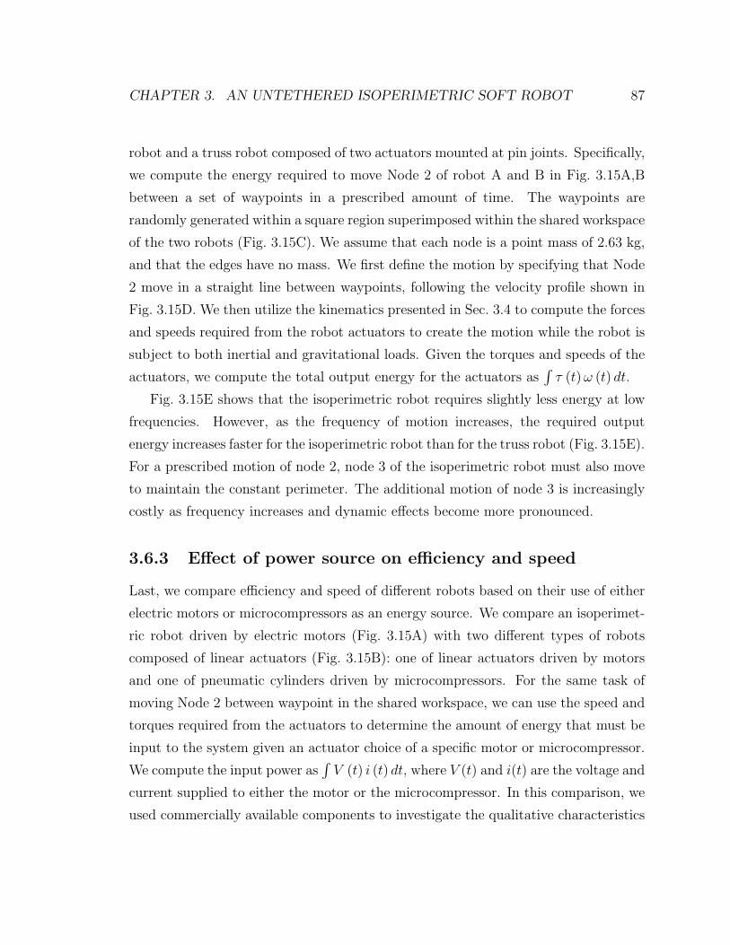
CHAPTER 3. AN UNTETHERED ISOPERIMETRIC SOFT ROBOT 87
robot and a truss robot composed of two actuators mounted at pin joints. Specifically,
we compute the energy required to move Node 2 of robot A and B in Fig. 3.15A,B
between a set of waypoints in a prescribed amount of time. The waypoints are
randomly generated within a square region superimposed within the shared workspace
of the two robots (Fig. 3.15C). We assume that each node is a point mass of 2.63 kg,
and that the edges have no mass. We first define the motion by specifying that Node
2 move in a straight line between waypoints, following the velocity profile shown in
Fig. 3.15D. We then utilize the kinematics presented in Sec. 3.4 to compute the forces
and speeds required from the robot actuators to create the motion while the robot is
subject to both inertial and gravitational loads. Given the torques and speeds of the
actuators, we compute the total output energy for the actuators as∫τ (t)ω (t) dt.
Fig. 3.15E shows that the isoperimetric robot requires slightly less energy at low
frequencies. However, as the frequency of motion increases, the required output
energy increases faster for the isoperimetric robot than for the truss robot (Fig. 3.15E).
For a prescribed motion of node 2, node 3 of the isoperimetric robot must also move
to maintain the constant perimeter. The additional motion of node 3 is increasingly
costly as frequency increases and dynamic effects become more pronounced.
3.6.3 Effect of power source on efficiency and speed
Last, we compare efficiency and speed of different robots based on their use of either
electric motors or microcompressors as an energy source. We compare an isoperimet-
ric robot driven by electric motors (Fig. 3.15A) with two different types of robots
composed of linear actuators (Fig. 3.15B): one of linear actuators driven by motors
and one of pneumatic cylinders driven by microcompressors. For the same task of
moving Node 2 between waypoint in the shared workspace, we can use the speed and
torques required from the actuators to determine the amount of energy that must be
input to the system given an actuator choice of a specific motor or microcompressor.
We compute the input power as∫V (t) i (t) dt, where V (t) and i(t) are the voltage and
current supplied to either the motor or the microcompressor. In this comparison, we
used commercially available components to investigate the qualitative characteristics
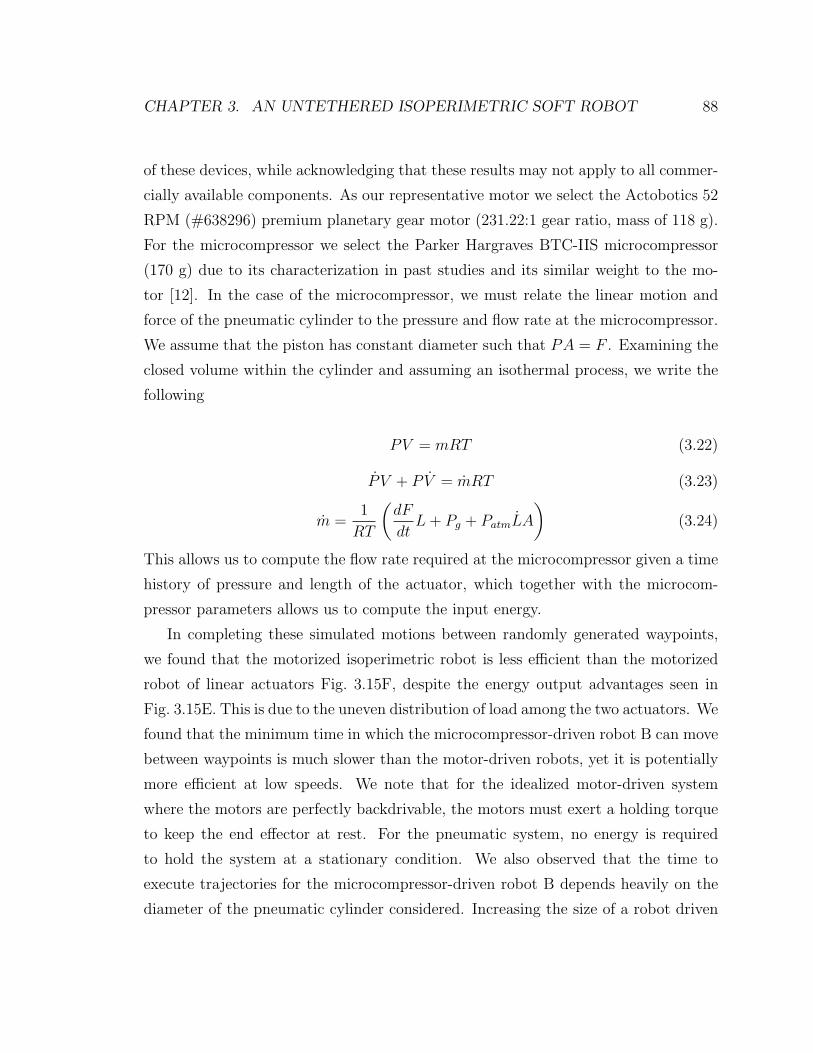
CHAPTER 3. AN UNTETHERED ISOPERIMETRIC SOFT ROBOT 88
of these devices, while acknowledging that these results may not apply to all commer-
cially available components. As our representative motor we select the Actobotics 52
RPM (#638296) premium planetary gear motor (231.22:1 gear ratio, mass of 118 g).
For the microcompressor we select the Parker Hargraves BTC-IIS microcompressor
(170 g) due to its characterization in past studies and its similar weight to the mo-
tor [12]. In the case of the microcompressor, we must relate the linear motion and
force of the pneumatic cylinder to the pressure and flow rate at the microcompressor.
We assume that the piston has constant diameter such that PA = F . Examining the
closed volume within the cylinder and assuming an isothermal process, we write the
following
PV = mRT (3.22)
P V + PV = mRT (3.23)
m =1
RT
(dF
dtL+ Pg + PatmLA
)(3.24)
This allows us to compute the flow rate required at the microcompressor given a time
history of pressure and length of the actuator, which together with the microcom-
pressor parameters allows us to compute the input energy.
In completing these simulated motions between randomly generated waypoints,
we found that the motorized isoperimetric robot is less efficient than the motorized
robot of linear actuators Fig. 3.15F, despite the energy output advantages seen in
Fig. 3.15E. This is due to the uneven distribution of load among the two actuators. We
found that the minimum time in which the microcompressor-driven robot B can move
between waypoints is much slower than the motor-driven robots, yet it is potentially
more efficient at low speeds. We note that for the idealized motor-driven system
where the motors are perfectly backdrivable, the motors must exert a holding torque
to keep the end effector at rest. For the pneumatic system, no energy is required
to hold the system at a stationary condition. We also observed that the time to
execute trajectories for the microcompressor-driven robot B depends heavily on the
diameter of the pneumatic cylinder considered. Increasing the size of a robot driven
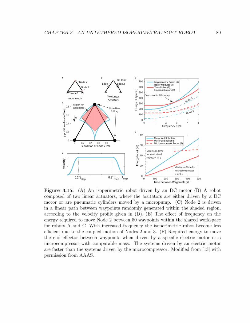
CHAPTER 3. AN UNTETHERED ISOPERIMETRIC SOFT ROBOT 89
0 0.2 0.4 0.6 0.8 1x position of node 2 (m)
0
0.2
0.4
0.6
0.8
y p
osi
tio
n o
f n
od
e 2
(m
)V
elo
city
tstep0.8*t0.2*t
stepstep
C
D
Node Mass2.63 kg
g
Region for Waypoints
Node 2
Node 3
Isoperimetric
Node 1
A
Two Linear
Actuators
Pin JointB
Edge 1 Edge 2
0 100 200 300 400 500Time Between Waypoints (s)
0
20
40
60
80En
erg
y In
pu
t (k
J)Motorized Robot (A)Motorized Robot (B)Microcompressor Robot (B)
0 1 2 3 4 5Frequency (Hz)
0
100
200
300
400
500
600
700
Ene
rgy
Ou
tpu
t (J
)
Isoperimetric Robot (A)Roller Modules (A)Truss Robot (B)Linear Actuators (B)
Crossover in Efficiency
Node 2
Node 3
E
F
Minimum Time
for motorized
robots = 11 s
Minimum Time for
microcompressor
= 273 s
Figure 3.15: (A) An isoperimetric robot driven by an DC motor (B) A robotcomposed of two linear actuators, where the acutators are either driven by a DCmotor or are pneumatic cylinders moved by a micropump. (C) Node 2 is drivenin a linear path between waypoints randomly generated within the shaded region,according to the velocity profile given in (D). (E) The effect of frequency on theenergy required to move Node 2 between 50 waypoints within the shared workspacefor robots A and C. With increased frequency the isoperimetric robot become lessefficient due to the coupled motion of Nodes 2 and 3. (F) Required energy to movethe end effector between waypoints when driven by a specific electric motor or amicrocompressor with comparable mass. The systems driven by an electric motorare faster than the systems driven by the microcompressor. Modified from [13] withpermission from AAAS.
CHAPTER 3. AN UNTETHERED ISOPERIMETRIC SOFT ROBOT 90
by a microcompressor increases the area the compressed gas exerts a pressure on,
effectively increasing the gear ratio: increasing the force output and reducing the
speed. This effect is observed in the untethered soft robot presented in [38]. The
authors built their robot at a relatively large scale (length of 0.65 m) to accommodate
commercially available compressors. The increase in size to accommodate commercial
components had the effect of reducing speed (reported speeds of about 18 m/hour or
28 body lengths/hour). Our robot is larger, but because it does not experience the
same effect of gear ratio change, it achieves faster locomotion speeds (216 m/hour or
128 body lengths/hour).
3.7 Discussion
In terms of softness, our robots differ from most devices in the field of soft robotics.
Although our robots are like most soft robots in that they comprise a mixture of
compliant materials (fabric and air) and some rigid components, they differ in that
their rigid components are external instead of internal. At first glance, this may
seem limiting, but it is a similar architecture to that found in insects, where rigid
exoskeletal segments are joined by compliant tissue [98]. In our case, the natural
compliance of the beams connecting the rigid nodes creates an effective stiffness that
is far below the actual stiffness of node material. Further, the mechanical fuse–type
behavior limits the overall maximum load that can be applied at a node. Naturally,
the compliant tubes afford some robustness to the roller modules because the tubes
can conform to misalignment of the rollers and prevent large forces and impacts from
being transmitted between roller modules. In addition, it may be possible in future
work to replace the roller modules with soft-bodied analogs to further increase the
safety and robustness of the system.
In this work, we presented versions of our robot at an approximately human scale.
A key question for understanding the broader applicability of this type of robot is
how performance changes with robot size scale. If we scale all dimensions uniformly,
then as the length L increases, the mass of the robot increases roughly with L3. The
strength of the structure is governed by the mechanics of inflated beams and is a

CHAPTER 3. AN UNTETHERED ISOPERIMETRIC SOFT ROBOT 91
function of the geometry, material properties, and internal pressure, which precludes
extracting a simple scaling law. If we assume that the strength of the structure can
be approximated by considering the inflated tubes as Euler beams that fail due to
buckling, the load-bearing capacity increases with L2, a slower rate of increase than
the robot’s mass, meaning that isometric upscaling will eventually result in robots
that cannot support their weight. However, given that buckling strength depends on
the fourth power of tube diameter, slightly positive allometric scaling of tube diameter
would enable increased robot sizes.
Our robotic concept is built upon a synthesis of concepts from collective, truss-
like, and soft robots. To design the primary component of the model, we developed
and validated a model that predicts the stiffness of a joint formed by a roller modular
and experimentally studied the effect of geometric parameters on the force required
to drive a roller along the tube. We extended the kinematic analysis from the pre-
vious chapter to the case where the the sums of some edges must remain constant.
We demonstrated the collective nature of the system by creating—from identical,
one-degree-of-freedom subunits—two 2D architectures and one 3D architecture. We
showed the robots’ truss-like behavior through marked shape change, load carrying,
and locomotion. We demonstrated and characterized their compliant nature through
a mechanical fuse behavior and an ability to engulf, grasp, and manipulate objects.
Last, we examined tradeoffs, comparing the workspace, efficiency, and speed of a robot
based on our concept to these characteristics of similar robots. Our work introduces
the isoperimetric concept to the field of soft robotics for the structure and movement
of untethered pneumatic robots, as well as presents a new mechanical architecture for
building truss robots. In the next chapter, we will present a distributed controller for
truss-like robots, further highlighting their ability to serve as a robot collective.
Chapter 4
Distributed Control of Truss
Robots Using Consensus
Alternating Direction Method of
Multipliers
4.1 Introduction
Modularity has been frequently cited as one of the important advantages of truss
robots [1, 4, 23]. In this chapter we consider truss robots as a collective, where many
individual members, each with their own sensing, computation, and actuation, coordi-
nate their motion to achieve desirable overall results. Research on robotic collectives
or swarms often draws inspiration from biological collectives such as swarms of fish,
birds, and insects, in which each member of the collective is capable of individual mo-
tion [99]. However, another type of collective exists in which individual components
of the swarm are physically connected into a structure, such as when colonies of ants
combine to form structures such as bridges or nests, or when slime mold organisms
aggregate and collectively locomote [100, 101, 102]. In a swarm where every agent is
physically disconnected, each member must be capable of moving on their own, and
the motion of each component is typically not directly altered by the motion of its
92
CHAPTER 4. DISTRIBUTED CONTROL OF TRUSS ROBOTS 93
neighbors. In a physically-interconnected collective, the shared connections impose
constraints on each member’s motion, and allows the motion of one component to
directly change the position of the other nodes throughout the collective. The coor-
dinated control of a physically interconnected collective thus poses additional control
challenges, while also allowing for a collective to achieve interesting behaviors — even
when the individual members are capable of only simple behaviors.
In this chapter we consider truss robots as physically interconnected collectives.
We focus this chapter on the general case of a truss robot composed of linear actuators
of controllable length connected at universal joints, , although these methods can also
be applied to the isoperimetric robots presented in Chapter 3. We define the nodes of
the system as the universal joints between edges, and assume that each node is capable
of computation and communication with the other nodes to which it is physically
connected with a linear actuator. We present distributed algorithms that allow each
node to determine the shape of the overall robot and coordinate their motions to
minimize a cost function and achieve desired motions, even if the desired motions are
only known to a subset of the nodes. In this chapter, we first define the problem and
provide an outline of our algorithm. We then present the mathematical underpinnings
of both the state estimation and control components of the algorithm, which are based
on a consensus formulation of alternating direction method of multipliers (ADMM)
with the ability to locally enforce constraints. We then apply these algorithms to
distributed state estimation for truss robots using local measurements at each node.
Next, we use the same ADMM framework to determine which control actions to
apply in order to achieve desired motion objectives. These control techniques build
upon the kinematics and centralized control algorithms presented in Chapter 2. We
demonstrate both state estimation and control in simulation.
4.1.1 Related Work
This chapter builds on past work on distributed control of truss robots. A key contri-
bution of the TETROBOT project was a set of modular control algorithms that work
in conjunction with modular hardware [20]. The distributed algorithms presented

CHAPTER 4. DISTRIBUTED CONTROL OF TRUSS ROBOTS 94
in [20] divide the nodes of the truss into two categories: controlled and unconstrained.
The unconstrained nodes move to minimize a cost function, and the controlled nodes
have a specified trajectory. The distributed algorithms use the chain-like kinematic
architecture of the robot to coordinate motions for each actuator, and also allow the
algorithms to account for dynamic effects [22]. However, these algorithms only allow
for specification of individual node motion. For example, in the controller of each
node it is impossible to control the motion of the center of mass, which is useful in
enabling locomotion.
Our work also builds on past work on distributed optimization. Our algorithms are
based on a consensus formulation of the alternating direction method of multipliers
(ADMM), which is discussed in detail in [103]. The ADMM framework allows for
the distributed solution of optimization problems. It is extended to a multi-agent
distributed computation framework in [104, 105]. Consensus ADMM has been used
for multi-target tracking [106]. In this work, we adapt consensus ADMM to include
the handling of linear constraints known to only a subset of the nodes, and apply
these results to both distributed estimation and control.
4.2 Problem Formulation and Algorithmic Sketch
We define the state of the robot in a fashion equivalent to Chapter 2. The truss robot
is defined as a framework that consists of a graph G and vertex positions pi ∈ Rd,
where d = 2, 3. The graph is denoted as G = {V , E}, where V = {1, . . . , n} are the
vertices of the graph and E = {. . . , {i, j}, . . .} are the undirected edges of the graph.
The geometry of the robot is fully represented by the concatenation of all vertex
positions x = [pT1 , pT2 , ..., p
Tn ]T . We define a length vector L, which is a concatenated
vector of the lengths of all edges in the graph:
Lk = ‖pi − pj‖ ∀ {i, j} ∈ E . (4.1)
The motions of the edges and the actuators are related through the expression

CHAPTER 4. DISTRIBUTED CONTROL OF TRUSS ROBOTS 95
Offboard Computer
PID
PID PID
PID
Task-Space Command
Linear Actuators
Computer/Module Communication
Module/Module Communication
(velocity commands in task space)
(estimated positions, planned velocities)
Node
NodeNode
Node
Figure 4.1: A schematic of the control architecture for the distributed truss robot.Each node takes local measurements and performs iterative communication with theneighboring nodes to determine the state of the robot and the local control actionthat it needs to take. It is also possible for external commands in task space to bebroadcast to a node, allowing a high-level planner or a human user to send commandsto the robot.
L = R(x)x, (4.2)
where R(x) is the scaled rigidity matrix first presented in Sec. 2.4.
We present distributed techniques that allow each node to determine the shape
of the overall robot, as well as methods to coordinate the control of the edge lengths
to achieved desired motion of the nodes. Our algorithms also allow a high-level
planner, or even a human operator, to send commands in task space. Each module
then coordinates its motion with its neighbors to ensure the overal robot achieves
this command. A schematic of this control architecture with the physical connections
between nodes, node-to-node communication, and the opportunity for communication
from an offboard source, is shown in Fig. 4.1. .
Algorithm 1 gives the overall structure of our algorithm. During each control
loop, each node first acquires measurements from its local sensors. The form of these
measurements will be discussed in Sec. 4.4, and may include the edge lengths of
the edges adjacent to the node, or the relative positions of neighboring nodes. This
information is used to complete an iterative ADMM optimization, where estimates
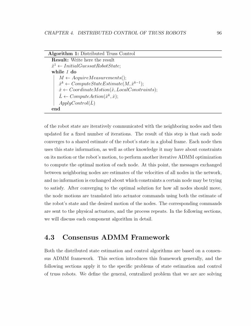
CHAPTER 4. DISTRIBUTED CONTROL OF TRUSS ROBOTS 96
Algorithm 1: Distributed Truss Control
Result: Write here the resultx1 ← InitialGuessatRobotState;while 1 do
M ← AcquireMeasurements();xk ← ComputeStateEstimate(M, xk−1);x← CoordinateMotion(x, LocalConstraints);
L← ComputeAction(xk, x);
ApplyControl(L)end
of the robot state are iteratively communicated with the neighboring nodes and then
updated for a fixed number of iterations. The result of this step is that each node
converges to a shared estimate of the robot’s state in a global frame. Each node then
uses this state information, as well as other knowledge it may have about constraints
on its motion or the robot’s motion, to perform another iterative ADMM optimization
to compute the optimal motion of each node. At this point, the messages exchanged
between neighboring nodes are estimates of the velocities of all nodes in the network,
and no information is exchanged about which constraints a certain node may be trying
to satisfy. After converging to the optimal solution for how all nodes should move,
the node motions are translated into actuator commands using both the estimate of
the robot’s state and the desired motion of the nodes. The corresponding commands
are sent to the physical actuators, and the process repeats. In the following sections,
we will discuss each component algorithm in detail.
4.3 Consensus ADMM Framework
Both the distributed state estimation and control algorithms are based on a consen-
sus ADMM framework. This section introduces this framework generally, and the
following sections apply it to the specific problems of state estimation and control
of truss robots. We define the general, centralized problem that we are are solving

CHAPTER 4. DISTRIBUTED CONTROL OF TRUSS ROBOTS 97
throughout this chapter as
minx
J(x) =n∑i=1
Ji(x) (4.3)
subject to Ax = b (4.4)
We distribute this problem across n computational nodes by having each node
maintain its own, local copy of the total state vector xi. We divide the cost function
into local components Ji(x) such that∑N
i=1 Ji(x) = J(x), and each node maintains
a local copy of a subset of the linear constraints Aixi = bi. Satisfaction of all of the
local constraints must ensure satisfaction of the constraints to the centralized problem
such that if x satisfies Aix = bi for all i, then x satisfies Ax = b.
Each node then solves the following optimization problem
minxi
Ji(xi) (4.5)
subject to Aixi = bi (4.6)
xi = xj, ∀j ∈ Ni. (4.7)
Equation 4.7 is a consistency constraint, that means that the copy of the state
vector at node i must equal the state vector at all neighboring nodes. Solving this
distributed problem then yields a solution that is equivalent to the solution to the cen-
tralized problem in Eqs. 4.3 and 4.4. To solve these coupled optimization problems,
we form the augmented Lagrangian
L =∑i∈V
(Ji(xi) + rTi (Ai − b) +
αr2‖Aixi − bi‖2 +
∑j∈N
[λTij(gij − xi) + νTij(gji − xj)]+
αp2
∑j∈Ni
(‖gi,j − xi‖2 + ‖gij − xj‖2
)),
(4.8)

CHAPTER 4. DISTRIBUTED CONTROL OF TRUSS ROBOTS 98
where gij are auxiliary primal variables that encode the consistency constraints, ri are
the Lagrange multipliers associated with the linear constraints, and λ and ν are the
Lagrange multipliers associated with the consistency constraints. The hyperparame-
ters αr and αp tune the sensitivity to disagreement between the neighbor’s estimates
and the violation of the local linear constraints. We then iteratively update each
set of variables in the augmented Lagrangian through a gradient ascent step on the
Lagrange multiplier variables (ν, λ, and r) and a minimization step of the primal
variables (x and g) as follows:
λ(k+1)ij = λ
(k)ij + αp
(g(k)ij − x
(k)i
)∀(i, j) ∈ E (4.9)
ν(k+1)ij = ν
(k)ij + αp
(g(k)ij − x
(k)j
)∀(i, j) ∈ E (4.10)
r(k+1)ij = r
(k)ij + αr
(Aix
(k)i − bi
)(4.11)
x(k+1) = argminx{L(x, r(k+1), g(k), λ
(k+1)ij , ν
(k+1)ij } (4.12)
g(k+1) = argming{L(xk+1, r(k+1), g, λ
(k+1)ij , ν
(k+1)ij } (4.13)
The update in Eq. 4.12 can be solved exactly in a distributed manner for each xi
because the augmented Lagrangian is separable. As shown in [104,105], substituting
pi =∑
j∈Niλij+νij and assuming the initialization p
(0)i = 0 causes Eq. 4.13 to become
gij =1
2(xi + xj). (4.14)
Using this expression we can rewrite the iterative steps Eqs. 4.9-4.13 in a manner in
which each agent can compute its updates in parallel as follows:

CHAPTER 4. DISTRIBUTED CONTROL OF TRUSS ROBOTS 99
pk+1i = pki + αp
∑j∈Ni
(xki − xkj ), (4.15)
rk+1i = rki + αr(Aix
ki − bi), (4.16)
xk+1i = argmin
xi
(Ji(xi) + (pk+1
i )Txi + (rk+1i )T (Aix
ki − bi)+
αp∑j∈Ni
∥∥∥∥∥xi − xki + xkj2
∥∥∥∥∥2
2
+ αr ‖Aixi − bi‖22).
(4.17)
Each agent iteratively perform these updates, which require each node to com-
municate their estimates of the state with the neighbors and solve the optimization
problem in Eq. 4.17. By performing these update steps iteratively, each agent only
communicates with its neighbors, and their estimates converge to a shared estimate
that satisfies the the local constraints. If J(x) is convex, then x(k)i will approach the
optimal centralized solution x∗ as the number of iterations increases to infinity.
4.3.1 Quadratic Cost Function
A special case that is relevant for our work is where the cost function Ji(x) is of the
quadratic form
Ji(xi) = ‖Dixi + fi‖2. (4.18)
This form allows us to compute the analytic solution to the optimization problem
in Eq. 4.17 as follows
xk+1i = M−1
(2αrA
Ti bi − pk+1
i − ATi rk+1i + αp
∑j∈Ni
(xki + xkj )
), (4.19)
where M is given by
M = Di(xi)TDi(xi) + 2αrA
Ti Ai + 2αpdi, (4.20)

CHAPTER 4. DISTRIBUTED CONTROL OF TRUSS ROBOTS 100
and di is the degree of each node. We note that because the updates in Eqs. 4.16-
4.17 are performed iteratively, the matrix M−1 is unchanged throughout the round of
iterations for a given problem. This allows for very efficient computation, because the
matrix inverse needs to be computed only once per problem, and then the updates
performed at each iteration only require multiplication of precomputed matrixes and
the current state estimates.
4.3.2 Convergence Criteria
Using the consensus ADMM approach to distributed optimization requires determin-
ing when to terminate the iterations. In a distributed setting, determining when a
stopping criteria is reached is challenging because each node does not have all of the
information. For example, if one node has converged and all constraints are satisfied,
this does not guarantee that another node, elsewhere in the network, has converged
on the proper solution. In addition, the convergence rate is also influenced by the
selection of the hyperparameters αp and αr. Throughout this chapter we empirically
select hyperparameters and run the optimization for a fixed number of iterations that
have empirically been demonstrated to result in good convergence. The fact that the
communication graph is set by the physical connections of the robot and does not
change indicates that the convergence behavior during experiments will be similar to
what would be observed on an actual robot.
4.4 Distributed State Estimation
We first consider the problem of state estimation, or the problem of determining
enough about the state of the robot to allow each node to plan and compute control
actions. The amount of information about the robot state required depends on the
amount of information needed to compute the local cost function Ji(x), translate a
planned motion into action, and evaluate any constraints. We select cost functions
that only require each agent to know its neighbors’ positions. Knowledge of positions
and planned motions of the neighboring nodes is sufficient to translate the planned
CHAPTER 4. DISTRIBUTED CONTROL OF TRUSS ROBOTS 101
motion into commands for each actuator. In Chapter 2 we discussed several types of
constraints: that actuator lengths stay within a maximum and minimum length, that
actuators do not collide, that the minimum angle between connected actuators remain
above a certain threshold, and that the robot remains in a configuration where it is
infinitesimally rigid. The constraint on the angles and actuator lengths only require
that each node have information about the neighboring nodes. The actuator collision
constraint requires that nodes are able to determine a region of potential collision,
which could also be achieved with local information. The final constraint we consider
in Chapter 2 is that the robot maintain infinitesimal rigidity, which corresponds to
avoiding singular configurations of the robot. In the general case, this constraint
requires that each node be aware of the location of nodes in the network that are
not its immediate neighbor. For this reason, we develop a distributed estimation
algorithm where each node reconstructs the entire state of the robot, and does so
by only using local measurements and then communicating estimates of the robot’s
state with the neighboring nodes. We evaluate the case where the nodes are able to
measure either the relative distance to the neighboring nodes, or the relative positions
of the neighboring nodes.
We also note that these algorithms are contingent on all of the nodes having
aligned reference frames. In practice this can be achieved by equipping each node
with an inertial measurement unit capable of measuring a gravity vector and a vector
indicating magnetic north. From these two vectors, it is possible to reconstruct an
aligned set of frames.
4.4.1 Sate estimation from relative position estimates
We first determine the overall configuration of the robot by assuming that each node
in the network is capable of computing estimates of the position of its neighbors in a
local reference frame. In a conventional truss robot, this naturally occurs if each node
has knowledge of the orientation and length of each incident edge. This measurement
could also be achieved if each node can visually determine the distance and position
of its neighbors. We express this relative position measurement as vi,j such that
CHAPTER 4. DISTRIBUTED CONTROL OF TRUSS ROBOTS 102
pi + vi,j = pj. Combining all of these expressions we obtain the following expression
which can be expressed as a summation over all of the nodes in the network
J(x) =n∑i
∑j∈Ni
‖pj − pi − vij‖2 =n∑i
Ji(x) (4.21)
This cost function is invariant to translation of the robot, which could create am-
biguity on how the robot is moving over time. We resolve this by including additional
linear constraints of the form Ax = b on the position of the nodes. One option is to
assume that the centroid of the robot is located at the origin, which is possible if we
express the constraint as 1T ⊗ I3x = 0. Alternatively, if we know the position of one
anchor node, referred to as node i, we can express the constraint as eTi ⊗ I3x = pi,
where ei is is an n× 1 vector of zeros where element i is equal to 1.
Combining the cost function in Eq. 4.21 and the linear constraints, we formulate
a distributed optimization problem of the form posed in Eqs. 4.5-4.7, which can be
solved through the iterative updates in Eqs. 4.16-4.17. This cost function is quadratic,
meaning that the optimization problem in Eq. 4.17 can be solved analytically using
Eq. 4.19, which leads to very efficient computation.
An important parameter is the number of relative position measurements neces-
sary to reconstruct the robot shape. Relative position measurements are sufficient to
reconstruct any connected graph, and a connected graph must have at least n − 1
edges. A robot must have at least n − 1 edges in order to be able to have a unique
solution to determining the global positions based on relative position measurements.
In practice, the truss robots are infinitesimally rigid, meaning that they have at least
3n − 6 edges in 3D and 2n − 3 edges in 2D, and thus there are redundant measure-
ments if all relative positions are measured. This strategy has the effect of using this
redundant information to improve the position estimate.
4.4.2 State estimation from relative distance measurements
Another option for reconstructing the global state of the robot is to assume that each
node knows its distance to all of the neighboring nodes, but not their positions. This

CHAPTER 4. DISTRIBUTED CONTROL OF TRUSS ROBOTS 103
is achieved if each node knows the lengths of all the adjacent actuators. In this case,
the cost function is expressed as
NL∑i=1
‖Li(x)− Lm,i‖2. (4.22)
We divide this cost between the computational nodes by having each node compute
the error based on only the adjacent edges. This cost function is invariant to both
translation and rotation. We remove this invariance by defining at least 6 linearly
independent constraints on the positions of the nodes which we express as Ax = b.
In practice we define these constraints in terms of the feet of the robot, or the nodes
of the robot that form the support polygon of the robot on the ground. In a physical
system these nodes could detect that they were on the ground using contact sensing.
We constrain one support foot to be fixed in three dimensions, a second support foot
to be fixed in both the vertical and one horizontal direction, and a third support foot
to be fixed in the vertical direction.
Similar to the case of relative positions, we combine the cost function and con-
straints. The cost function in Eq. 4.22 is nonconvex, indicating that several local
minima may exist. This cost function is exactly equivalent to reconstructing a graph
based on its edge lengths, a key problem in rigidity theory that is discussed in some
depth in Chapter 2. Depending on the number of edges, different classes of solutions
may exist. For truss robots, we consider only graphs that are minimally rigid or over-
constrained because those are the only graphs where the node motion can be fully
controlled by changing the edge lengths. If the graph is minimally rigid, there are
3n − 6 edges, which constitute the minimum number of edges to fix the position of
the nodes. However, this also means that there is no redundant information that can
be utilized to reduce the effect of noisy measurements. Additional edges in the graph
that lead to the graph being overconstrained could allow for improved behavior under
noisy measurements. We also note that each iteration of the update procedure with
the distance objective function requires solving the nonlinear optimization problem
using an iterative numeric solver. This leads to substantially slower performance than
the analytic solution to the quadratic optimization problem presented in Eq. 4.21.

CHAPTER 4. DISTRIBUTED CONTROL OF TRUSS ROBOTS 104
4.4.3 Comparison between estimation schemes
We have presented two algorithms for state estimation, one that utilizes relative
position information to each neighbor, and another that utilizes relative distance in-
formation. A drawback of using relative position estimates is that it requires that
more information be gathered in the measurements, but is also has several advantages:
the optimization problem has a unique solution, redundant information is incorpo-
rated to reduce the effect of noisy measurements, and it is computationally efficient
because the optimization that is part of each iteration can be solved analytically.
The estimation scheme using relative distance leads to an optimization problem that
could potentially have multiple solutions, and may not include any tolerance to noisy
measurements. In Sec. 4.6.1 we will use simulation to further compare these two ap-
proaches. A key point is that during the iterative state estimation routine, the nodes
communicate only their estimates of the global state with their neighbors, and do not
communicate their measurements directly. This potentially increases the generality
of the algorithm, because other types of measurements could be incorporated in the
cost function or constraints at each node, while the information exchanged between
nodes remains the same.
4.5 Distributed Control Algorithm
We now present a distributed algorithm that allows the nodes of the robot to de-
termine how to coordinate the motion of the actuators to minimize a cost function
while satisfying constraints. In the previous section, the nodes complete an ADMM
optimization where the decision variable is the location of each nodes in a shared ref-
erence frame. For the case of control, the decision variable is a vector of the velocity of
each of the node, x. Controlling in the space of velocities provides a natural method
to encode behavior and also simplifies the treatment of constraints. We express the
physical feasibility constraints as a function of the position of the nodes, f(x) < 0.
While the constraints f(x) < 0 are nonlinear, the derivative of these constraints is
linear in the velocity of the nodes df(x)dt
= ∂f(x)∂x
x. Our approach is to compute which

CHAPTER 4. DISTRIBUTED CONTROL OF TRUSS ROBOTS 105
constraints are active, and then use our algorithm to enforce the linear constraint
that the nodes do not move along the gradient direction of increasing constraint vi-
olation. A key advantage of the distributed approach is that constraint information
can be held locally at each node, and none of the other nodes need to be aware of a
constraint for it to be obeyed. For example, if a user seeks to teleoperate the robot,
velocity commands can be sent to a single node of the robot and used as a local linear
constraint to ensure that the node satisfies the specified motion. No other node of the
robot needs to know the command. If a truss robot is moving autonomously through
a cluttered environment and one node is close to colliding with an external obstacle,
the node can enforce a constraint to stop moving in a given direction. Despite the fact
the no other nodes are aware of the obstacle, the distributed control algorithm will
ensure that no other node moves in a way that violates the constraint. In addition,
constraints that involve many nodes will be obeyed even if they are sent to a subset of
the nodes. For example, a constraint that the center of mass move with a particular
velocity can be broadcast to one or more of the nodes, and the optimization will
ensure that all nodes move in a way that satisfies the constraint.
For the case of control, we consider two different cost functions. Each deals with
a cost that is computed as a sum of costs for each actuator. We distribute this cost
by having each node consider the cost of all adjacent actuators.
J(x) = ‖L(x)‖ = ‖R(x)x‖2 =n∑i=1
‖Li,j∈Ni(x)‖ (4.23)
The second objective seeks to minimize the deviance of the edges from some nominal
edge length. This behavior can be expressed through the following cost function,
which is a function of the position of the nodes
‖L(x)− Lnominal‖2 (4.24)
where Lnominal is a vector of the nominal length of each edge. However, our control
algorithm requires a command in terms of the velocities, and not positions. To
translate this concept of maintaining nominal edge lengths to an objective that is a
function of velocity, we use as the cost function the norm squared of the difference
CHAPTER 4. DISTRIBUTED CONTROL OF TRUSS ROBOTS 106
between the velocity and the gradient of Eq. 4.24
‖x− (L(x)− Lnominal)TRT (x)‖2. (4.25)
In addition to the cost function, we also impose the constraints that the ground
feet of the robot remain stationary as
Cx = 0. (4.26)
We can also encode any other constraint that is linear in the velocity of nodes and
is of the form
Ax = b. (4.27)
If we use the mass matrix for A, this allows us to control the center of mass of the
robot. We can also define the A matrix to specify the velocity of a certain node if it
of the form [0, 0, I3, 0]
To perform the control, we select either the cost function given in Eq. 4.24 or
Eq. 4.25, and a set of local constraints to define the following optimization problem:
minxi
Ji(xi) (4.28)
subject to[Ai
Ci
]xi =
[bi
0
](4.29)
xi = xj, ∀j ∈ Ni, (4.30)
where xi is the estimate at node i of the velocity of all nodes of the robot.
4.6 Simulation Results
We validate the algorithm via simulation. We first present results on state estimation,
and then results on the control algorithms.
CHAPTER 4. DISTRIBUTED CONTROL OF TRUSS ROBOTS 107
4.6.1 State Estimation
To examine the performance of the state estimation algorithms, we performed simu-
lations using both the cost function in which each node measures the relative position
of the neighboring nodes (Eq. 4.21), and the cost function where each agent measures
the distance to the neighboring nodes (Eq. 4.22). Figure 4.2 shows the results for
both techniques using several different levels of noise in the measurements of either
the distances or relative positions. We choose an octahedral robot shape, and per-
turb it slightly from its nominal configuration by starting all edges at a length of 1 m,
then increasing or decreasing the lengths based on a distance generated by a normal
distribution with 0 mean and variance of 0.25 m. This allows us to demonstrate that
the resulting convergence does not leverage the symmetry of a uniform graph. Both
cost functions use linear constraints to fix the height of all three support feet, in ad-
dition to fixing the x and y position of one foot and the y position of the third foot.
We complete 200 rounds of the ADMM iterations to minimize the cost function and
satisfy the constraints using the updates in Eqs. 4.16-4.17. We perform three differ-
ent trials, increasing the variance of normally distributed noise that we use for the
measurements. For the relative position estimates we use the analytic solution shown
in Eq. 4.19. When using the relative distance measurements, we use MATLAB’s
fminunc solver to solve the optimization in Eq. 4.17. To increase computation speed
of the fminunc solver, we analytically compute the gradient of the objective function
and provide it to the solver to speed convergence. We perform all computation on a
laptop computer (Intel Core i7 Processor, 4 cores, 2.80 GHz, 16GB RAM).
The top row of Fig. 4.2 shows the results based on relative distances, and the
bottom row shows results for relative positions, while each column corresponds to a
different level of noise injected into the measurements. For the case of low noise, both
results converge to a solution that appears approximately identical to the nominal
shape of the graph. To quantify the closeness of the fit, we compute the average error
as the average distance between each node’s estimated and true position. As the noise
level increases, the average error of both estimation schemes increases. Overall, the
error using the relative position measurements (Eq. 4.21) is lower than for relative
distances (Eq. 4.22). This is expected, because the relative position measurements

CHAPTER 4. DISTRIBUTED CONTROL OF TRUSS ROBOTS 108
Measurement Noise σ=0.01m
Reconstructed Con�guration from Relative Positions
Reconstructed Con�guration from
Edge Lengths
Measurement Noise σ=0.10m Measurement Noise σ=0.20m
Figure 4.2: The reconstructed state with varying levels of noise injected into themeasurements. The top row shows the state estimate when each node measures itsrelative distance to its neighbors. The bottom row shows the state estimate wheneach node measures the relative position of each of its neighbors. With increasingnoise, the estimate using relative position information produces better estimates. Inaddition, the relative position information allows far more efficient computation.
contain more information than the relative distance measurements. Another key dif-
ference between these two optimizations is the computation time. Using the relative
position measurements and the resulting quadratic cost function, the maximum dura-
tion of the 200 iterations was 0.071 seconds. Using the relative distance measurements
requires completing the iterative optimization using fminunc every time step, and led
to a maximum computation time of 9.43 seconds.
One challenge of state estimation with relative distance measurements is the pos-
sible existence of multiple solutions. For the case of relative position measurements,
there is a unique minimizer to the objective function that satisfies the constraints.
However, for the case of relative distance measurements, there are potentially other
configurations that also minimize the cost function. To examine this effect, we re-
peat the previous experiments, but instead of adding noise to the measurements, we
instead added noise to the initial guess. We added normally distributed noise with 0
mean, and ran the optimization at different levels of variance ranging from 0.1 m to
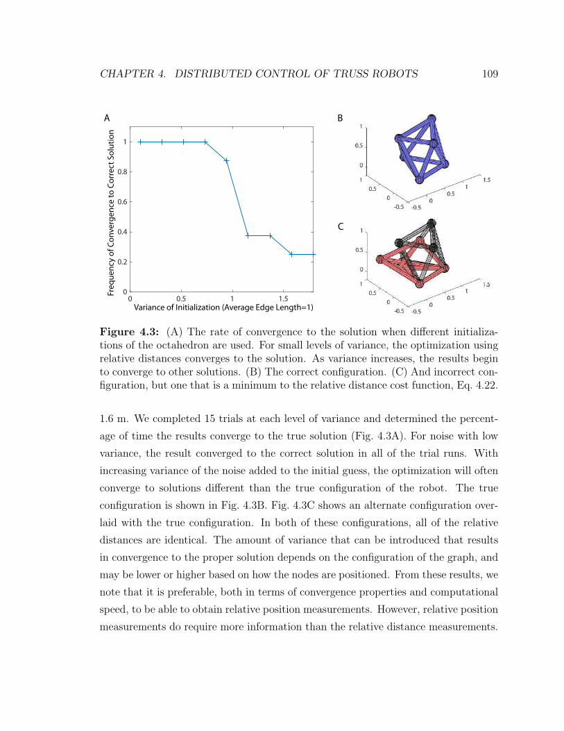
CHAPTER 4. DISTRIBUTED CONTROL OF TRUSS ROBOTS 109
0 0.5 1 1.5Variance of Initialization (Average Edge Length=1)
BA
C
0
0.2
0.4
0.6
0.8
1
Fre
qu
en
cy o
f C
on
verg
en
ce t
o C
orr
ect
So
luti
on
Figure 4.3: (A) The rate of convergence to the solution when different initializa-tions of the octahedron are used. For small levels of variance, the optimization usingrelative distances converges to the solution. As variance increases, the results beginto converge to other solutions. (B) The correct configuration. (C) And incorrect con-figuration, but one that is a minimum to the relative distance cost function, Eq. 4.22.
1.6 m. We completed 15 trials at each level of variance and determined the percent-
age of time the results converge to the true solution (Fig. 4.3A). For noise with low
variance, the result converged to the correct solution in all of the trial runs. With
increasing variance of the noise added to the initial guess, the optimization will often
converge to solutions different than the true configuration of the robot. The true
configuration is shown in Fig. 4.3B. Fig. 4.3C shows an alternate configuration over-
laid with the true configuration. In both of these configurations, all of the relative
distances are identical. The amount of variance that can be introduced that results
in convergence to the proper solution depends on the configuration of the graph, and
may be lower or higher based on how the nodes are positioned. From these results, we
note that it is preferable, both in terms of convergence properties and computational
speed, to be able to obtain relative position measurements. However, relative position
measurements do require more information than the relative distance measurements.

CHAPTER 4. DISTRIBUTED CONTROL OF TRUSS ROBOTS 110
4.6.2 Distributed Control
In this section, we simulate the distributed control algorithm that uses the robot
state as a starting point, and determines the velocities with which all nodes move.
We consider a 2D truss robot consisting of 9 actuators and 6 nodes as shown in
Fig. 4.5A. We assign the initial task of moving the top node (node 6) to move with
a velocity of 1 m/s in the x direction, while the cost function for the optimization
is Eq. 4.24. We show the evolution of each node’s estimate of all nodes’ planned
velocities during one round of ADMM updates in Fig. 4.4. The results demonstrate
that as all agents converge to identical estimates, the constraint violation decreases,
and the cost function converges to the minimizer of the centralized problem. The
solution to the centralized problem is found by solving the optimization in Eqs. 4.3-
4.4 with identical cost function and constraints.
We now evaluate the performance of the control scheme over multiple rounds
of ADMM updates and when the controller is used in conjunction with the state
estimation scheme described in Sec. 4.4. Fig. 4.5 shows the performance of the robot
when the tasks is to move the top node with a velocity of 1 m/s in the x direction for
2 seconds, and then reverse the velocity. Each node measures the relative position
of their neighboring nodes, and then reconstructs the state. For the control, we use
the cost function in Eq. 4.25, fix the position of the bottom left node in both the
horizontal and vertical directions, and the position of the bottom center node in
the vertical direction as illustrated in Fig. 4.5A. This task is performed open-loop,
with the command being to always move with a constant velocity in the x direction,
regardless of whether past errors have occurred. The behavior of the robot without
noise is shown in Fig. 4.5A.
To evaluate the behavior in a realistic scenario, we add noise to the measurements
each node takes of the relative position of its neighboring nodes. We use these noisy
measurements to compute the estimated robot state and the control action, and then
we apply the control to the actual state of the robot. The noise is normally distributed
with 0 mean and variances of 0.01 m, 0.25 m, and 0.50 m. The trajectories of the
top node, as well as the final configuration of the robot, are shown in Fig. 4.5C. The
velocity of the top node is also shown in Fig. 4.5(B and C). With increasing noise,

CHAPTER 4. DISTRIBUTED CONTROL OF TRUSS ROBOTS 111
0 50 100 150 200 250Iteration
0
0.5
1Node 1Node 2Node 3Node 4Node 5Node 6Centralized Optimum
0 50 100 150 200 250Iteration
10-10
10-5
100
0 50 100 150 200 250Iteration
0
1
2
3
4
5
No
de
6 S
pe
ed
Est
imat
eC
on
stra
int
Vio
lati
on
Co
st (e
q. 4
.21
)
A
B
C
Figure 4.4: Convergence of each node’s estimated state. (A) The estimate main-tained by each node of the velocity of node 6. All estimates converge to an identicalvalue. (B) The maximum violations of the local constraints at each node. In thiscase, only node 6 (the top node) and nodes 1 and 2 (the base nodes) have activeconstraints. (C) The centralized cost evaluated based on each agent’s estimate. Allagents converge to the same solution, which is identical to the solution obtained bysolving the centralized optimization.
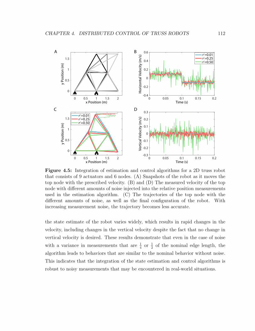
CHAPTER 4. DISTRIBUTED CONTROL OF TRUSS ROBOTS 112
=0.50
A B
C D
=0.01=0.25
2
2
2
=0.50
=0.01=0.25
2
2
2
Figure 4.5: Integration of estimation and control algorithms for a 2D truss robotthat consists of 9 actuators and 6 nodes. (A) Snapshots of the robot as it moves thetop node with the prescribed velocity. (B) and (D) The measured velocity of the topnode with different amounts of noise injected into the relative position measurementsused in the estimation algorithm. (C) The trajectories of the top node with thedifferent amounts of noise, as well as the final configuration of the robot. Withincreasing measurement noise, the trajectory becomes less accurate.
the state estimate of the robot varies widely, which results in rapid changes in the
velocity, including changes in the vertical velocity despite the fact that no change in
vertical velocity is desired. These results demonstrate that even in the case of noise
with a variance in measurements that are 14
or 12
of the nominal edge length, the
algorithm leads to behaviors that are similar to the nominal behavior without noise.
This indicates that the integration of the state estimation and control algorithms is
robust to noisy measurements that may be encountered in real-world situations.
CHAPTER 4. DISTRIBUTED CONTROL OF TRUSS ROBOTS 113
4.7 Conclusion
This chapter presented distributed control algorithms for truss robots composed of
linear actuators connected at universal joints. These algorithms, based on a consensus
ADMM framework, allow the nodes to coordinate their behavior across the entire
network while only communicating locally with their physical neighbors. Each agent
uses an iterative ADMM update to reconstruct the state of the entire network during
the state estimation phase while exchanging messages that are each agents estimate
of the global state. During the control phase, the ADMM updates are performed
on the estimated velocity of each node. In the case of a quadratic cost function,
the updates are extremely efficient computationally. However, they do require many
rounds of communication. In these results, all communication was simulated within
the same computer. Achieving this high communication load in a distributed manner
in a physical robot may be a significant engineering challenge.
The control approach presented in this chapter coordinates motions of the actu-
ators of a truss robot to achieve a set of desired node motions, but these methods
do not determine what the desired node motions should be. A separate high-level
planner could be developed to provide the desired motions. The approach of sep-
arating the motion specification and the coordination of the actuators’ motion can
potentially simplify the planning problem for the high-level planner, as it would only
need to plan for the motion of a subset of the robot’s nodes. The desired motions
could alternatively be provided by a human operator, who could teleoperate one node
or the center of mass of the robot using a joystick. The desired motions could also be
generated based on sensor information obtained locally at each node. For example, if
a node observes a target with an onboard camera, that node could decide to move the
center of mass in the direction of the target. Future work can examine these different
methods to specify the desired motion.
In the current system, each agent reasons about the position and desired velocity
of all other nodes in the network. This means that the size of the messages passed
between neighbors grows linearly with the number of agents in the network, even if
the number of neighbors stays the same. Also, this system requires that all agents

CHAPTER 4. DISTRIBUTED CONTROL OF TRUSS ROBOTS 114
have aligned frames. Some of these requirements could be relaxed to increase the
applicability of these distributed algorithms.
Chapter 5
Conclusion
This dissertation presents control techniques for truss robots, as well the design of a
novel isoperimetric truss robot. In this chapter we summarize the major contributions
and discuss opportunities for future work.
5.1 Review of Contributions
The main contributions of this dissertation are as follows:
• Kinematics and control techniques for general linear actuator robots.
In Chapter 2 we characterized the kinematics of arbitrary robots consisting of
linear actuators connected together at universal joints, as well as the physical
constraints that must be satisfied to ensure the robots are physically feasible.
We presented an optimization-based control technique that minimizes either the
required actuator motion or the deviance from a nominal configuration while
satisfying physical constraints and ensuring that specified motions are achieved.
This optimization can be solved online for arbitrary networks and enables the
actuators to move the center of mass of the robot along a trajectory. For robots
of certain symmetry, solving this optimization offline enables the computation
of repeated gaits.
• Development of a new isoperimetric robot and characterization of its
115

CHAPTER 5. CONCLUSION 116
capabilities. In Chapter 3 we presented a new type of soft truss robot that
we call an “isoperimetric” robot. The robot is composed of inflated tubes that
pass through a set of roller modules. These modules pinch the tube to create
an area of locally reduced bending stiffness which acts as a rotational joint.
The robot changes shape by driving the joints along the tube. This changes
the relative edge lengths but maintains the overall perimeter and hence the
inflated volume of the robot. The robot can then operate without a pressure
source. We discussed the mechanical design of the roller modules, including
a model that predicts the torque required to bend the beam when the roller
module is present. We modified the kinematics from Chapter 2 to include the
constraint that the total edge length remain constant. We demonstrated the
robot changing shape, locomoting using a punctuated rolling gait, and grasping
and manipulating objects. We presented three different robot configurations
using an identical set of roller modules.
• A distributed controller for truss robots. In Chapter 4 we presented a
distributed controller for truss robots that allows all the nodes to coordinate
their actions, despite each node only communicating with its neighboring nodes.
This algorithm solves distributed optimization problems using the consensus al-
ternating direction of multipliers to both determine the overall state of the robot
and what actions must be taken by each each actuator. This framework allows
each node to incorporate local constraints, without explicitly communicating
these constraints throughout the network.
5.2 Future Work
5.2.1 Design Improvements
A key avenue of future work is determining which types of robots can be constructed
using the isoperimetric paradigm. The types of robots constructed can vary in size,
number of modules, and topology, as well as the desired task of the robot. We will
discuss each of these aspects in further detail.
CHAPTER 5. CONCLUSION 117
The overall size of the robot affects the robot’s ability to support external loads
and its ability to support loads caused by the robot’s own weight. In Chapter 3 we
discuss that if we increase the edge length L and all other dimensions of the robot
uniformly, the mass of the robot increases with L3, and the load-bearing capability
increases with approximately L2. These scaling laws predict that the robot grows
stronger relative to its weight as the size decreases. Future work could characterize
the limits on how small the robot could be. It is possible that the availability of
miniature components such as batteries, motors, and gears may limit the practicality
of building the device at a small scale. The abilities of the robot may also be limited
due to the increased prevalence of frictional effects and resistance to air flow between
modules that occurs at small size scales. Miniature isoperimetric robots may allow for
the inclusion of large numbers of modules to create a device capable of high resolution
shape change. At a smaller size scale, it may also be possible to design isoperimetric
devices capable of operating within the human body as potential medical devices.
We also consider the effect of increasing the size of robot. If all dimensions are
scaled uniformly, the robot becomes weaker relative to its weight as it increases in size.
However, increasing the diameter d of the inflated tubes increases the load bearing
capability with d4, indicating that it is possible to create larger robots by increasing
the diameter of the tubes at a faster rate than increasing the lengths of the edges.
This could enable large scale robots capable of supporting their own body weight,
and potentially applications where the robot serves as a type of active structure.
An obvious avenue for future work is to increase the number of modules in the
robot, allowing for more controlled degrees of freedom and a higher degree of shape
change. A key challenge for systems with more modules is the increased weight that
must be supported by some of the members, especially the base members, if they are
supporting a number of modules in the air above them. One option is to move from a
homogeneous system, where the sizes of all tubes and roller modules are identical, to
a heterogeneous system, where the edges that may experience high load are composed
of larger diameter tubes.
Adding more modules to the robot also requires characterizing the topologies of
trusses that can serve as isoperimetric robots. A key characteristic of the current

CHAPTER 5. CONCLUSION 118
system is that the roller modules pinch the tube between two cylinders, creating a
planar joint that cannot rotate about the long axis of the tube. This requires that
the angle between adjacent sets of roller modules relative to the tube must remain
constant during operation. This has led many of our current designs to be composed
of tubes routed in triangular paths, which are guaranteed to remain planar and satisfy
this constraint. This poses a significant restriction on the types of robots that can be
created using an isoperimetric system. Future work could characterize precisely what
types of trusses can be decomposed into triangles, such that each edge of the truss is
part of exactly one triangle.
While characterizing the topologies of robots that can be created with the current
roller modules would be valuable, a new type of roller module would enable new
topologies. The constraint that a fixed angle is maintained between adjacent roller
modules could be relaxed through the design of a roller module that creates a universal
joint, as opposed to a planar joint. A universal joint would be created by a roller
module that pinches the tube by causing it to pass through a ring-like structure. In
addition to increasing the variety of robots that could be built, this would allow robots
to have more extreme shape change, as the constraint that each triangle maintains
the same perimeter would be relaxed to the constraint that the entire robot maintains
the same perimeter, a significant reduction in the constraints on possible shapes.
In this dissertation our algorithms have controlled a robot with predefined topol-
ogy to perform a task. In the future, algorithms could be developed to perform
topological design of the robot to perform a task or set of tasks. This algorithm could
iteratively consider adding more modules to the robot to create designs where the
physical structure is designed to facilitate task completion. It is also possible that if
the objective is to build a robot for a specific task, the isoperimetric system could be
combined with other types of robotic systems. For example, if object manipulation
were the target application, an isoperimetric system could be built as an end effector
for a conventional robotic arm. The robot arm could account for gross position, and
the truss system could dramatically change shape to cage objects, adjust to complex
geometry, or even spin objects within the grasp.
CHAPTER 5. CONCLUSION 119
5.2.2 Control and Modeling Improvements
In addition to changes in the mechanical design of the robot, future work could also
expand the capabilities of truss robots through improved control techniques. Here we
discuss future work where the controller directly considers the the loading condition,
compliance, and dynamics of the robot.
One significant advancement to our current control techniques would be to directly
consider the loading condition of the robot when planning control actions. As noted
in the previous section, a key barrier to increasing the number of modules in the robot
or performing certain tasks is the fact that the inflated beams fail due to buckling.
While some of this may be addressed through mechanical design, the loading can
also be reduced by controlling the robot to configurations that naturally reduce the
loading on the most vulnerable members. An optimization-based controller, similar
to those presented in Chapters 2 and 4, could be used with an objective function that
gives a high cost when edges of the robot are close to a specified failure criterion. It
may also be possible to instrument the connections between modules of the physical
robot with force sensors, and actively measure force information that can be used to
control the robot to reduce loading.
Another potential area of future work is to develop a model of the robot geometry
that takes into account the compliance and deformation of the robot. The current
modeling and control techniques presented in this dissertation assume that the length
of an actuator exactly specifies the distance between two nodes, or equivalently, that
the robot is perfectly rigid. In the case of the inflated beams of the isoperimetric
robot, this model may be inaccurate in two ways. First, there is some bending and
compliance of the inflated beams when they are placed under load. Second, if a beam
is under high load, it is possible that the beam buckles, creating a new buckle point
that acts as an effective joint in the structure. Future work could develop a model of
the robot that accounts both for the compliance and the dramatic buckling events.
Such a model could also allow for the robot to detect failures due to buckling, and
then move in a way that allows the robot to recover from these failures.
Finally, future control techniques could account for and leverage the dynamic
behavior of the robot. The current model of the system used for control assumes
CHAPTER 5. CONCLUSION 120
that the motion of the robot is quasistatic, meaning that no dynamic effects are
present. While our current system changes shape at a rate slow enough that dynamic
effects do not significantly contribute to the robot’s behavior, future robots could
move faster, increasing the importance of dynamic effects. Also, for certain behaviors
such as tipping over and rolling, our robot experiences unmodeled dynamic effects.
Future control design could leverage the dynamic behavior of the robot to enable more
efficient versions of current behavior (for example, punctuated rolling while leveraging
the dynamic effects during toppling) or to design new behaviors that leverage dynamic
effects (for example, enabling the robot to jump).
Bibliography
[1] S. Curtis, M. Brandt, G. Bowers, G. Brown, C. Cheung, C. Cooperider, M. De-
sch, N. Desch, J. Dorband, K. Gregory, K. Lee, A. Lunsford, F. Minetto,
W. Truszkowski, R. Wesenber, J. Vranish, M. Abrahantes, P. Clark, T. Capon,
W. Michael, R. Watson, P. Olivier, and M. L. Rilee, “Tetrahedral robotics for
space exploration,” IEEE Aerospace and Electronic Systems Magazine, vol. 22,
no. 6, pp. 22–30, 2007.
[2] A. Spinos, D. Carroll, T. Kientz, and M. Yim, “Variable topology truss: Design
and analysis,” in IEEE/RSJ International Conference on Intelligent Robots and
Systems, pp. 2717–2722, 2017.
[3] D. Rus and M. T. Tolley, “Design, fabrication and control of soft robots,”
Nature, vol. 521, no. 7553, pp. 467–475, 2015.
[4] G. J. Hamlin and A. C. Sanderson, “Tetrobot modular robotics: Prototype
and experiments,” in Proc. IEEE/RSJ International Conference on Intelligent
Robots and Systems, pp. 390–395, 1996.
[5] A. Spinos and M. Yim, “Towards a variable topology truss for shoring,” in
Proc. IEEE Ubiquitous Robots and Ambient Intelligence, pp. 244–249, 2017.
[6] M. Alexa, D. Cohen-Or, and D. Levin, “As-rigid-as-possible shape interpola-
tion,” in 27th annual conference on Computer Graphics and Interactive Tech-
niques. ACM Press/Addison-Wesley Publishing Co., 2000, pp. 157–164.
[7] C. Majidi, “Soft robotics: a perspective—current trends and prospects for the
future,” Soft Robotics, vol. 1, no. 1, pp. 5–11, 2014.
121
BIBLIOGRAPHY 122
[8] E. Steltz, A. Mozeika, N. Rodenberg, E. Brown, and H. M. Jaeger, “Jsel: Jam-
ming skin enabled locomotion,” in IEEE/RSJ International Conference on In-
telligent Robots and Systems, 2009, pp. 5672–5677.
[9] R. F. Shepherd, F. Ilievski, W. Choi, S. A. Morin, A. A. Stokes, A. D. Mazzeo,
X. Chen, M. Wang, and G. M. Whitesides, “Multigait soft robot,” Proceedings
of the National Academy of Sciences, vol. 108, no. 51, pp. 20 400–20 403, 2011.
[10] M. T. Tolley, R. F. Shepherd, M. Karpelson, N. W. Bartlett, K. C. Galloway,
M. Wehner, R. Nunes, G. M. Whitesides, and R. J. Wood, “An untethered
jumping soft robot,” in IEEE/RSJ International Conference on Intelligent
Robots and Systems, 2014, pp. 561–566.
[11] J. Fras, Y. Noh, M. Macias, H. Wurdemann, and K. Althoefer, “Bio-inspired
octopus robot based on novel soft fluidic actuator,” in IEEE International Con-
ference on Robotics and Automation, 2018, pp. 1583–1588.
[12] M. Wehner, M. T. Tolley, Y. Menguc, Y.-L. Park, A. Mozeika, Y. Ding, C. Onal,
R. F. Shepherd, G. M. Whitesides, and R. J. Wood, “Pneumatic energy sources
for autonomous and wearable soft robotics,” Soft Robotics, vol. 1, no. 4, pp.
263–274, 2014.
[13] N. S. Usevitch, Z. M. Hammond, M. Schwager, A. M. Okamura, E. W. Hawkes,
and S. Follmer, “An untethered isoperimetric soft robot,” Science Robotics,
vol. 5, no. 40, 2020.
[14] Y. Patel, P. George, et al., “Parallel manipulators applications—a survey,” Mod-
ern Mechanical Engineering, vol. 2, no. 03, p. 57, 2012.
[15] B. Dasgupta and T. Mruthyunjaya, “The stewart platform manipulator: a re-
view,” Mechanism and Machine Theory, vol. 35, no. 1, pp. 15–40, 2000.
[16] B. K. Wada, J. L. Fanson, and E. F. Crawley, “Adaptive structures,” Journal
of Intelligent Material Systems and Structures, vol. 1, no. 2, pp. 157–174, 1990.

BIBLIOGRAPHY 123
[17] V. A. Reinholtz and L. T. Watson, “Enumeration and analysis of variable ge-
ometry truss manipulators,” 1990.
[18] M. D. Rhodes and M. Mikulas Jr, “Deployable controllable geometry truss
beam,” NASA Technical Memorandum, no. 86366, 1985.
[19] P. C. Hughes, W. G. Sincarsin, and K. A. Carroll, “Trussarm—a variable-
geometry-truss manipulator,” Journal of Intelligent Material Systems and
Structures, vol. 2, no. 2, pp. 148–160, 1991.
[20] G. J. Hamlin and A. C. Sanderson, “Tetrobot: A modular approach to parallel
robotics,” IEEE Robotics & Automation Magazine, vol. 4, no. 1, pp. 42–50,
1997.
[21] W. H. Lee and A. C. Sanderson, “Dynamics and distributed control of tetrobot
modular robots,” IEEE International Conference on Robotics and Automation,
vol. 4, pp. 2704–2710, 1999.
[22] W. H. Lee and A. Sanderson, “Dynamic rolling locomotion and control of mod-
ular robots,” IEEE Transactions on Robotics and Automation, vol. 18, no. 1,
pp. 32–41, 2002.
[23] C.-H. Yu, K. Haller, D. Ingber, and R. Nagpal, “Morpho: A self-deformable
modular robot inspired by cellular structure,” IEEE/RSJ International Con-
ference on Intelligent Robots and Systems, pp. 3571–3578, 2008.
[24] J. C. Zagal, C. Armstrong, and S. Li, “Deformable octahedron burrowing
robot,” In Proc. Int. Conf. on the Synthesis and Simulation of Living Systems,
pp. 431–438, 2012.
[25] A. Mazzone and A. Kunz, “Sketching the future of the smartmesh wide area
haptic feedback device by introducing the controlling concept for such a de-
formable multi-loop mechanism,” Links, vol. 3, p. 248, 2005.
[26] R. Kovacs, A. Ion, P. Lopes, T. Oesterreich, J. Filter, P. Otto, T. Arndt,
N. Ring, M. Witte, A. Synytsia, et al., “Trussformer: 3D printing large kinetic
BIBLIOGRAPHY 124
structures,” Proc. ACM Symposium on User Interface Software and Technology,
pp. 113–125, 2018.
[27] M. Pieber, R. Neurauter, and J. Gerstmayr, “An adaptive robot for building in-
plane programmable structures,” IEEE International Conference on Intelligent
Robots and Systems, pp. 5320–5327, 2018.
[28] A. Sofla, D. Elzey, and H. Wadley, “Shape morphing hinged truss structures,”
Smart Materials and Structures, vol. 18, no. 6, pp. 065 012–065 020, 2009.
[29] A. Lyder, R. F. M. Garcia, and K. Stoy, “Mechanical design of odin, an extend-
able heterogeneous deformable modular robot,” IEEE/RSJ Intelligent Robots
and Systems, pp. 883–888, 2008.
[30] F. Collins and M. Yim, “Design of a spherical robot arm with the spiral zip-
per prismatic joint,” in Proc. IEEE International Conference on Robotics and
Automation, pp. 2137–2143, 2016.
[31] Z. Hammond, N. Usevitch, E. Hawkes, and S. Follmer, “Pneumatic reel actu-
ator: Design, modeling, and implementation,” IEEE International Conference
on Robotics and Automation, pp. 883–888, 2017.
[32] M. Zhang, X. Geng, J. Bruce, K. Caluwaerts, M. Vespignani, V. SunSpiral,
P. Abbeel, and S. Levine, “Deep reinforcement learning for tensegrity robot lo-
comotion,” in Proc. IEEE International Conference on Robotics and Automa-
tion, pp. 634–641, 2017.
[33] J. Bruce, A. P. Sabelhaus, Y. Chen, D. Lu, K. Morse, S. Milam, K. Caluwaerts,
A. M. Agogino, and V. SunSpiral, “Superball: Exploring tensegrities for
planetary probes,” in 12th International Symposium on Artificial Intelligence,
Robotics, and Automation in Space, 2014.
[34] A. P. Sabelhaus, J. Bruce, K. Caluwaerts, P. Manovi, R. F. Firoozi, S. Dobi,
A. M. Agogino, and V. SunSpiral, “System design and locomotion of superball,

BIBLIOGRAPHY 125
an untethered tensegrity robot,” in IEEE International Conference on Robotics
and Automation, 2015, pp. 2867–2873.
[35] J. Friesen, A. Pogue, T. Bewley, M. de Oliveira, R. Skelton, and V. Sunspiral,
“Ductt: A tensegrity robot for exploring duct systems,” in IEEE International
Conference on Robotics and Automation, 2014, pp. 4222–4228.
[36] E. W. Hawkes and M. R. Cutkosky, “Design of materials and mechanisms for
responsive robots,” Annual Review of Control, Robotics, and Autonomous Sys-
tems, vol. 1, pp. 359–384, 2018.
[37] S. I. Rich, R. J. Wood, and C. Majidi, “Untethered soft robotics,” Nature
Electronics, vol. 1, no. 2, pp. 102–112, 2018.
[38] M. T. Tolley, R. F. Shepherd, B. Mosadegh, K. C. Galloway, M. Wehner,
M. Karpelson, R. J. Wood, and G. M. Whitesides, “A resilient, untethered
soft robot,” Soft Robotics, vol. 1, no. 3, pp. 213–223, 2014.
[39] R. Niiyama, D. Rus, and S. Kim, “Pouch motors: Printable/inflatable soft
actuators for robotics,” in IEEE International Conference on Robotics and Au-
tomation, 2014, pp. 6332–6337.
[40] A. D. Marchese, C. D. Onal, and D. Rus, “Autonomous soft robotic fish capable
of escape maneuvers using fluidic elastomer actuators,” Soft Robotics, vol. 1,
no. 1, pp. 75–87, 2014.
[41] M. Wehner, R. L. Truby, D. J. Fitzgerald, B. Mosadegh, G. M. Whitesides,
J. A. Lewis, and R. J. Wood, “An integrated design and fabrication strategy
for entirely soft, autonomous robots,” Nature, vol. 536, no. 7617, pp. 451–455,
2016.
[42] M. Loepfe, C. M. Schumacher, U. B. Lustenberger, and W. J. Stark, “An un-
tethered, jumping roly-poly soft robot driven by combustion,” Soft Robotics,
vol. 2, no. 1, pp. 33–41, 2015.

BIBLIOGRAPHY 126
[43] M. Yim, W.-M. Shen, B. Salemi, D. Rus, M. Moll, H. Lipson, E. Klavins, and
G. S. Chirikjian, “Modular self-reconfigurable robot systems,” IEEE Robotics
& Automation Magazine, vol. 14, no. 1, pp. 43–52, 2007.
[44] H. Ahmadzadeh, E. Masehian, and M. Asadpour, “Modular robotic systems:
characteristics and applications,” Journal of Intelligent & Robotic Systems,
vol. 81, no. 3-4, pp. 317–357, 2016.
[45] L. Krick, M. E. Broucke, and B. A. Francis, “Stabilisation of infinitesimally rigid
formations of multi-robot networks,” International Journal of Control, vol. 82,
no. 3, pp. 423–439, 2009.
[46] N. Usevitch, Z. Hammond, and M. Schwager, “Locomotion of linear actuator
robots through kinematic planning and nonlinear optimization,” Transactions
on Robotics, vol. In Press, 2020.
[47] M. Abrahantes, A. Silver, and L. Wendt, “Gait design and modeling of a 12-
tetrahedron walker robot,” Proc. IEEE Southeastern Symposium on System
Theory, pp. 21–25, 2007.
[48] X. Wang, X. Wang, Z. Zhang, and Y. Zhao, “Motion planning of kinemat-
ically redundant 12-tetrahedral rolling robot,” International Journal of Ad-
vanced Robotic Systems, vol. 13, no. 1, p. 23, 2016.
[49] X. Wang, X. Wang, and Z. Zhang, “Dynamical modelling and a decentral-
ized adaptive controller for a 12-tetrahedral rolling robot,” Transactions of FA-
MENA, vol. 42, no. 2, pp. 51–66, 2018.
[50] S. Jeong, B. Kim, S. Park, E. Park, A. Spinos, D. Carroll, T. Tsabedze,
Y. Weng, T. Seo, M. Yim, F. C. Park, and J. Kim, “Variable topology truss:
Hardware overview, reconfiguration planning and locomotion,” in Proc. IEEE
International Conference on Ubiquitous Robots (UR), pp. 616–621, 2018.
BIBLIOGRAPHY 127
[51] K. Kim, A. K. Agogino, A. Toghyan, D. Moon, L. Taneja, and A. M. Agogino,
“Robust learning of tensegrity robot control for locomotion through form-
finding,” in IEEE/RSJ International Conference on Intelligent Robots and Sys-
tems, 2015, pp. 5824–5831.
[52] C. Paul, F. J. Valero-Cuevas, and H. Lipson, “Design and control of tensegrity
robots for locomotion,” IEEE Transactions on Robotics, vol. 22, no. 5, pp.
944–957, 2006.
[53] A. P. Sabelhaus, A. H. Li, K. A. Sover, J. R. Madden, A. R. Barkan, A. Agogino,
and A. Agogino, “Inverse statics optimization for compound tensegrity robots,”
IEEE Robotics and Automation Letters, vol. In Press, 2020.
[54] X. Xu, F. Sun, Y. Luo, and Y. Xu, “Collision-free path planning of tensegrity
structures,” Journal of Structural Engineering, vol. 140, no. 4, p. 04013084,
2013.
[55] S. M. LaValle and J. J. Kuffner Jr, “Randomized kinodynamic planning,” The
International Journal of Robotics Research, vol. 20, no. 5, pp. 378–400, 2001.
[56] Z. Littlefield, K. Caluwaerts, J. Bruce, V. SunSpiral, and K. E. Bekris, “Inte-
grating simulated tensegrity models with efficient motion planning for planetary
navigation,” in International Symposium on Artificial Intelligence, Robotics,
and Automation in Space, 2016.
[57] Z. Littlefield, D. Surovik, W. Wang, and K. E. Bekris, “From quasi-static to kin-
odynamic planning for spherical tensegrity locomotion,” in Robotics Research.
Springer, 2020, pp. 947–966.
[58] C. Paul, J. W. Roberts, H. Lipson, and F. V. Cuevas, “Gait production in a
tensegrity based robot,” in Proceedings of IEEE the International Conference
on Advanced Robotics. IEEE, 2005, pp. 216–222.
[59] A. Iscen, A. Agogino, V. SunSpiral, and K. Tumer, “Controlling tensegrity
robots through evolution,” in Proceedings of the 15th Annual Conference on
Genetic and Evolutionary Computation, 2013, pp. 1293–1300.
BIBLIOGRAPHY 128
[60] J. Rieffel and J.-B. Mouret, “Adaptive and resilient soft tensegrity robots,” Soft
Robotics, vol. 5, no. 3, pp. 318–329, 2018.
[61] C. Rennie and K. E. Bekris, “Discovering a library of rhythmic gaits for spher-
ical tensegrity locomotion,” in IEEE International Conference on Robotics and
Automation, 2018, pp. 2290–2295.
[62] K. Caluwaerts, M. D’Haene, D. Verstraeten, and B. Schrauwen, “Locomotion
without a brain: physical reservoir computing in tensegrity structures,” Artifi-
cial Life, vol. 19, no. 1, pp. 35–66, 2013.
[63] B. Cera and A. M. Agogino, “Multi-cable rolling locomotion with spherical
tensegrities using model predictive control and deep learning,” in IEEE/RSJ
International Conference on Intelligent Robots and Systems, 2018, pp. 1–9.
[64] D. Surovik, K. Wang, M. Vespignani, J. Bruce, and K. E. Bekris, “Adaptive
tensegrity locomotion: Controlling a compliant icosahedron with symmetry-
reduced reinforcement learning,” The International Journal of Robotics Re-
search, pp. 1–22, 2019.
[65] M. Vespignani, C. Ercolani, J. Friesen, and J. Bruce, “Steerable locomotion con-
troller for six-strut icosahedral tensegrity robots,” in Proc. IEEE International
Conference on Intelligent Robots and Systems, pp. 2886–2892, 2018.
[66] K. Caluwaerts, J. Despraz, A. Iscen, A. P. Sabelhaus, J. Bruce, B. Schrauwen,
and V. SunSpiral, “Design and control of compliant tensegrity robots through
simulation and hardware validation,” Journal of the Royal Society Interface,
vol. 11, no. 98, p. 20140520, 2014.
[67] N. Usevitch, Z. Hammond, S. Follmer, and M. Schwager, “Linear actuator
robots: Differential kinematics, controllability, and algorithms for locomotion
and shape morphing,” in Proc. IEEE/RSJ International Conference on Intel-
ligent Robots and Systems, pp. 5361–5367, 2017.

BIBLIOGRAPHY 129
[68] S. Park, E. Park, M. Yim, J. Kim, and T. Seo, “Optimization-based nonimpact
rolling locomotion of a variable geometry truss,” IEEE Robotics and Automation
Letters, vol. 4, no. 2, pp. 747–752, 2019.
[69] L. Asimow and B. Roth, “The rigidity of graphs,” Transactions of the American
Mathematical Society, vol. 245, pp. 279–289, 1978.
[70] S. Pellegrino and C. R. Calladine, “Matrix analysis of statically and kinemat-
ically indeterminate frameworks,” International Journal of Solids and Struc-
tures, vol. 22, no. 4, pp. 409–428, 1986.
[71] E. G. Gilbert, D. W. Johnson, and S. S. Keerthi, “A fast procedure for comput-
ing the distance between complex objects in three-dimensional space,” IEEE
Journal on Robotics and Automation, vol. 4, no. 2, pp. 193–203, 1988.
[72] D. Zelazo, A. Franchi, H. H. Bulthoff, and P. Robuffo Giordano, “Decentralized
rigidity maintenance control with range measurements for multi-robot systems,”
The International Journal of Robotics Research, vol. 34, no. 1, pp. 105–128,
2015.
[73] D. Zelazo, A. Franchi, F. Allgower, H. H. Bulthoff, and P. R. Giordano, “Rigid-
ity maintenance control for multi-robot systems,” Robotics: Science and Sys-
tems, pp. 473–480, 2012.
[74] M. H. Trinh, M.-C. Park, Z. Sun, B. D. Anderson, V. H. Pham, and H.-S. Ahn,
“Further analysis on graph rigidity,” in Proc. IEEE Conference on Decision
and Control, pp. 922–927, 2016.
[75] H. Gluck, “Almost all simply connected closed surfaces are rigid,” Geometric
Topology, pp. 225–239, 1975.
[76] S. M. LaValle, Planning Algorithms. Cambridge University Press, 2006.
[77] M. Takeichi, K. Suzumori, G. Endo, and H. Nabae, “Development of a 20-
m-long giacometti arm with balloon body based on kinematic model with air
BIBLIOGRAPHY 130
resistance,” in IEEE/RSJ International Conference on Intelligent Robots and
Systems, 2017, pp. 2710–2716.
[78] S. Voisembert, A. Riwan, N. Mechbal, and A. Barraco, “A novel inflatable robot
with constant and continuous volume,” in 2011 IEEE International Conference
on Robotics and Automation, 2011, pp. 5843–5848.
[79] Y. A. Seong, R. Niiyama, Y. Kawahara, and Y. Kuniyoshi, “Low-pressure soft
inflatable joint driven by inner tendon,” in 2nd IEEE International Conference
on Soft Robotics (Robosoft), 2019, pp. 37–42.
[80] A. Stilli, H. A. Wurdemann, and K. Althoefer, “A novel concept for safe,
stiffness-controllable robot links,” Soft Robotics, vol. 4, no. 1, pp. 16–22, 2017.
[81] H. Sareen, U. Umapathi, P. Shin, Y. Kakehi, J. Ou, H. Ishii, and P. Maes,
“Printflatables: printing human-scale, functional and dynamic inflatable ob-
jects,” in Proceedings of the CHI Conference on Human Factors in Computing
Systems, 2017, pp. 3669–3680.
[82] S. Swaminathan, M. Rivera, R. Kang, Z. Luo, K. B. Ozutemiz, and S. E.
Hudson, “Input, output and construction methods for custom fabrication of
room-scale deployable pneumatic structures,” Proceedings of the ACM on In-
teractive, Mobile, Wearable and Ubiquitous Technologies, vol. 3, no. 2, pp. 1–17,
2019.
[83] J. W. Romanishin, K. Gilpin, and D. Rus, “M-blocks: Momentum-driven, mag-
netic modular robots,” in IEEE/RSJ International Conference on Intelligent
Robots and Systems, 2013, pp. 4288–4295.
[84] G. Jing, T. Tosun, M. Yim, and H. Kress-Gazit, “An end-to-end system for
accomplishing tasks with modular robots.” in Robotics: Science and Systems,
2016, pp. 1–5.
[85] F. Nigl, S. Li, J. E. Blum, and H. Lipson, “Structure-reconfiguring robots:
Autonomous truss reconfiguration and manipulation,” IEEE Robotics & Au-
tomation Magazine, vol. 20, no. 3, pp. 60–71, 2013.
BIBLIOGRAPHY 131
[86] S.-k. Yun, D. A. Hjelle, E. Schweikardt, H. Lipson, and D. Rus, “Planning the
reconfiguration of grounded truss structures with truss climbing robots that
carry truss elements,” in IEEE International Conference on Robotics and Au-
tomation, 2009, pp. 1327–1333.
[87] B. Jenett, A. Abdel-Rahman, K. Cheung, and N. Gershenfeld, “Material–robot
system for assembly of discrete cellular structures,” IEEE Robotics and Au-
tomation Letters, vol. 4, no. 4, pp. 4019–4026, 2019.
[88] K. H. Petersen, R. Nagpal, and J. K. Werfel, “Termes: An autonomous robotic
system for three-dimensional collective construction,” Robotics: Science and
Systems VII, 2011.
[89] C. R. Nesler, T. A. Swift, and E. J. Rouse, “Initial design and experimental
evaluation of a pneumatic interference actuator,” Soft Robotics, vol. 5, no. 2,
pp. 138–148, 2018.
[90] J. Fay and C. Steele, “Bending and symmetric pinching of pressurized tubes,”
International Journal of Solids and Structures, vol. 37, no. 46-47, pp. 6917–
6931, 2000.
[91] K. Wakana, H. Namari, M. Konyo, and S. Tadokoro, “Pneumatic flexible hollow
shaft actuator with high speed and long stroke motion,” in IEEE International
Conference on Robotics and Automation, 2013, pp. 357–363.
[92] B. A. Baydere, S. K. Talas, and E. Samur, “A novel highly-extensible 2-dof
pneumatic actuator for soft robotic applications,” Sensors and Actuators A:
Physical, vol. 281, pp. 84–94, 2018.
[93] R. L. Foote, “The volume swept out by a moving planar region,” Mathematics
Magazine, vol. 79, no. 4, pp. 289–297, 2006.
[94] W. Fichter, A theory for inflated thin-wall cylindrical beams. National Aero-
nautics and Space Administration, 1966, vol. 3466.
BIBLIOGRAPHY 132
[95] R. Comer and S. Levy, “Deflections of an inflated circular-cylindrical cantilever
beam,” AIAA Journal, vol. 1, no. 7, pp. 1652–1655, 1963.
[96] Y. He and W. Chen, “Experiment and theoretical analysis study of etfe inflat-
able tubes,” International Journal of Aerospace Engineering, pp. 1–10, 2014.
[97] T. Yoshikawa, “Manipulability of robotic mechanisms,” The International Jour-
nal of Robotics Research, vol. 4, no. 2, pp. 3–9, 1985.
[98] S. A. Wainwright, W. Biggs, J. Gosline, and J. Currey, Mechanical design in
organisms. Princeton University Press, 1982.
[99] Y. Mohan and S. Ponnambalam, “An extensive review of research in swarm
robotics,” in IEEE World Congress on Nature & Biologically Inspired Comput-
ing, 2009, pp. 140–145.
[100] M. Malley, B. Haghighat, L. Houel, and R. Nagpal, “Eciton robotica: Design
and algorithms for an adaptive self-assembling soft robot collective,” in IEEE
International Conference on Robotics and Automation, vol. In Press, 2020.
[101] F. Mondada, L. M. Gambardella, D. Floreano, S. Nolfi, J.-L. Deneuborg, and
M. Dorigo, “The cooperation of swarm-bots: Physical interactions in collective
robotics,” IEEE Robotics & Automation Magazine, vol. 12, no. 2, pp. 21–28,
2005.
[102] T. Umedachi, K. Takeda, T. Nakagaki, R. Kobayashi, and A. Ishiguro, “Fully
decentralized control of a soft-bodied robot inspired by true slime mold,” Bio-
logical Cybernetics, vol. 102, no. 3, pp. 261–269, 2010.
[103] S. Boyd, N. Parikh, E. Chu, B. Peleato, and J. Eckstein, “Distributed optimiza-
tion and statistical learning via the alternating direction method of multipliers,”
Foundations and Trends in Machine Learning, vol. 3, no. 1, pp. 1–122, 2011.
[104] T.-H. Chang, M. Hong, and X. Wang, “Multi-agent distributed optimization
via inexact consensus admm,” IEEE Transactions on Signal Processing, vol. 63,
no. 2, pp. 482–497, 2014.
BIBLIOGRAPHY 133
[105] G. Mateos, J. A. Bazerque, and G. B. Giannakis, “Distributed sparse linear
regression,” IEEE Transactions on Signal Processing, vol. 58, no. 10, pp. 5262–
5276, 2010.
[106] O. Shorinwa, J. Yu, T. Halsted, A. Koufos, and M. Schwager, “Dis-
tributed multi-target tracking for autonomous vehicle fleets,” arXiv preprint
arXiv:2004.05965, 2020.