Design and Analysis of Digital Direct-Detection Fiber ...optcom/Dissertations/Dissertation...Design...

Design and Analysis of Digital Direct-Detection Fiber-Optic CommunicationSystems Using Volterra Series Approach

A Dissertation

Presented to

the Faculty of the School of Engineering and Applied Science

University of Virginia

In Partial Fulfillment

of the requirements for the Degree of

Doctor of Philosophy

(Electrical Engineering)

by

Kumar V. Peddanarappagari

October, 1997

Abstract

Optical fiber communication systems are the most efficient means of handling the heavy data

traffic in this information age. Efforts are being made to increase the already phenomenal capacity

of these high bandwidth communication systems. Highly coherent optical sources that can generate

high power narrow pulses are being developed and fiber amplifiers are making repeaterless transmis-

sion over long distances possible. Considerable attention is being paid to the limitations placed on

these systems by linear dispersion, fiber nonlinearities, and amplified spontaneous emission (ASE)

noise from fiber amplifiers. However, most of the analysis is based on single pulse-propagation

experiments and simplified analytical expressions; pulse-to-pulse interactions are generally ignored.

The design of these systems is still empirical due to lack of analytical expressions for the output field

in terms of input, fiber, and amplifier parameters. This study develops analytical tools to analyze

and design systems to reduce the influence of linear dispersion, fiber nonlinearities, and ASE noise

in single-user and multi-user systems.

The generalized nonlinear Schroedinger (NLS) wave equation may be used to explain the effects

of linear dispersion and fiber nonlinearities on the evolution of the complex envelope of the optical

field in an optical fiber. The NLS equation is typically solved using numerical (recursive) methods.

In this work, a Volterra series based nonlinear transfer function of an optical fiber is derived based

on solving the NLS equation in the frequency-domain and retaining only the most significant terms

(Volterra kernels) in the resulting transfer function. Single pulse-propagation in single-mode optical

fibers is studied and the results are compared to available literature which uses numerical solutions.

The linear portion of the above model is then used for the theoretical study of the effects of

phase noise on linear dispersion in single-mode fiber-optic communication systems using a direct-

detection receiver. The effect of coherence time on dispersion, nonlinear interference (pulse-to-

pulse interactions), and intensity noise on the performance of a single-user communication system

is studied. A study of the effects of phase uncertainty in the received pulses due to timing jitter in

ii

modern lasers is also presented.

Using the Volterra series transfer function (VSTF), the effects of linear dispersion and fiber

nonlinearities on the performance of single-user fiber-optic communication systems are studied;

the criterion used is the signal-to-interference ratio (SIR) of intensity of the optical field and an

upper bound on the probability of error at the receiver. The model helps us choose input pulse

parameters to maximize the SIR (minimize probability of error) and design the complete optical

link or design lumped nonlinear equalizers at the receiver to compensate for the effects of linear

dispersion and fiber nonlinearities. Using the analytical expressions provided by the VSTF and the

upper bound on the probability of error, optimal dispersion parameters for the fiber segments in a

fiber amplifier based optical communication system are obtained to minimize the linear dispersion,

fiber nonlinearities and ASE noise. The effect of input power levels and amplifier gains on the system

performance in several different possible configurations of a point-to-point optical communication

system is studied. Finally, useful mathematical expressions for studying the nonlinear effects in

WDM systems are derived and possible ways of optimally extracting the information transmitted by

different users are discussed.

iii

Contents

1 Introduction 1

1.1 Fiber-optic Communication Systems . . . . . . . . . . . . . . . . . . . . . . . . . 1

1.2 Optical Transmitter . . . . . . . . . . . . . . . . . . . . . . . . . . . . . . . . . . 3

1.3 Optical Fiber . . . . . . . . . . . . . . . . . . . . . . . . . . . . . . . . . . . . . 6

1.3.1 Linear Attenuation . . . . . . . . . . . . . . . . . . . . . . . . . . . . . . 7

1.3.2 Linear (Chromatic) Dispersion . . . . . . . . . . . . . . . . . . . . . . . . 8

1.3.3 Fiber Nonlinearities . . . . . . . . . . . . . . . . . . . . . . . . . . . . . 10

1.4 Optical Amplifiers . . . . . . . . . . . . . . . . . . . . . . . . . . . . . . . . . . 13

1.5 Optical Receiver . . . . . . . . . . . . . . . . . . . . . . . . . . . . . . . . . . . 15

1.6 System Analysis and Design . . . . . . . . . . . . . . . . . . . . . . . . . . . . . 16

1.7 Dissertation Organization . . . . . . . . . . . . . . . . . . . . . . . . . . . . . . . 20

2 Signal Degradations within Fiber-optic Systems 22

2.1 Degradations Caused by Laser Source Imperfections . . . . . . . . . . . . . . . . 22

2.2 Degradations Caused by the Optical Fiber . . . . . . . . . . . . . . . . . . . . . . 25

2.2.1 Nonlinear Schroedinger Wave Equation . . . . . . . . . . . . . . . . . . . 26

2.2.2 Linear Dispersion . . . . . . . . . . . . . . . . . . . . . . . . . . . . . . . 30

2.2.3 Nonlinear Phenomenon . . . . . . . . . . . . . . . . . . . . . . . . . . . . 31

2.2.4 Optical Amplifiers . . . . . . . . . . . . . . . . . . . . . . . . . . . . . . 35

2.3 Photo-detector and Receiver . . . . . . . . . . . . . . . . . . . . . . . . . . . . . 37

iv

2.4 Performance Evaluation . . . . . . . . . . . . . . . . . . . . . . . . . . . . . . . . 38

3 Volterra Series Transfer Function (VSTF) 40

3.1 Derivation of Volterra Series Transfer Function . . . . . . . . . . . . . . . . . . . 43

3.2 Numerical Results . . . . . . . . . . . . . . . . . . . . . . . . . . . . . . . . . . . 48

3.3 Potential Applications . . . . . . . . . . . . . . . . . . . . . . . . . . . . . . . . . 55

3.3.1 Two-signal Analysis . . . . . . . . . . . . . . . . . . . . . . . . . . . . . 55

3.3.2 Nonlinear Equalizer . . . . . . . . . . . . . . . . . . . . . . . . . . . . . 59

3.3.3 Optimal Input Parameters . . . . . . . . . . . . . . . . . . . . . . . . . . 61

3.4 Summarized Observations . . . . . . . . . . . . . . . . . . . . . . . . . . . . . . 67

4 Linear Dispersion in Fiber-optic Communications 68

4.1 Derivation of SIR for Arbitrary Light Source . . . . . . . . . . . . . . . . . . . . . 69

4.1.1 Completely Coherent Light . . . . . . . . . . . . . . . . . . . . . . . . . 72

4.1.2 Completely Incoherent Light . . . . . . . . . . . . . . . . . . . . . . . . . 73

4.2 Numerical Results . . . . . . . . . . . . . . . . . . . . . . . . . . . . . . . . . . . 74

4.2.1 Communication System Performance . . . . . . . . . . . . . . . . . . . . 78

4.3 Summarized Observations . . . . . . . . . . . . . . . . . . . . . . . . . . . . . . 87

5 System Design 89

5.1 Transfer Function of the System . . . . . . . . . . . . . . . . . . . . . . . . . . . 91

5.2 Receiver Statistics . . . . . . . . . . . . . . . . . . . . . . . . . . . . . . . . . . . 95

5.3 Modified Chernoff Bound (MCB) . . . . . . . . . . . . . . . . . . . . . . . . . . 98

5.4 Design Example . . . . . . . . . . . . . . . . . . . . . . . . . . . . . . . . . . . . 101

5.5 Concluding Remarks . . . . . . . . . . . . . . . . . . . . . . . . . . . . . . . . . 108

6 Conclusions and Future Work 110

6.1 Summary . . . . . . . . . . . . . . . . . . . . . . . . . . . . . . . . . . . . . . . 110

v

6.2 Future Work . . . . . . . . . . . . . . . . . . . . . . . . . . . . . . . . . . . . . . 112

A Analysis of WDM Systems Using VSTF method 116

vi

List of Figures

1.1 A block diagram of a typical fiber-optic communication system. . . . . . . . . . . 3

3.1 Normalized square deviation of the output field for no Raman effect and no dis-

persion for different input peak powers. The SSF method from the true solution is

shown with lines, the third-order VSTF method from the true solution is shown with

’ � ’, and the fifth-order VSTF method from the true solution is shown with ’+’. . . 50

3.2 Normalized square deviation of the output field for no Raman effect for different

input peak powers the third-order VSTF method from the SSF method, shown with

lines, and the fifth-order VSTF method from the SSF method, shown with ’ � ’. . . 52

3.3 Magnitude squared of the Fourier transform of output field. . . . . . . . . . . . . . 53

3.4 Normalized square deviation of the output field of third- (shown with lines) and fifth-

order VSTF method (shown with ’ � ’) from SSF method, showing the dependence

of NSD on input RMS pulse-width for a length of ��

km. . . . . . . . . . . . 54

3.5 Interference-to-signal ratio due to the presence of a pump pulse at different frequencies. 58

3.6 Plots of output intensity of completely coherent light for different power levels. . . 62

3.7 Plot of RMS widths of output pulses, showing the effect of peak input power on

dispersion of the input pulse. . . . . . . . . . . . . . . . . . . . . . . . . . . . . . 63

3.8 Output SIR as a function of symbol period for different power levels. . . . . . . . . 65

3.9 Output SIR as a function of peak pulse power for different symbol periods. . . . . 66

vii

4.1 Output pulse shapes for different levels of coherence of light for input pulses of�

psec RMS width: (a) GVD dominant case (b) operation at zero-dispersion wave-

length, �� . . . . . . . . . . . . . . . . . . . . . . . . . . . . . . . . . . . . . . . . 75

4.2 Plot of RMS pulse-widths of output pulses, showing the effect of coherence time on

dispersion: (a) GVD dominant case (b) operation at zero-dispersion wavelength, �� . 77

4.3 Plots of different waveforms of expected received signal (signal and mean nonlinear

interference) and �� showing the effect of pulse separation on the nonlin-

ear interference: (a) GVD dominant case (b) operation at zero-dispersion wavelength. 79

4.4 Plot of SIR � , SIR �� , SIR �� , SIR � , and SIR �� showing the effect of coherence time

and timing jitter for a fixed symbol period of � � psec and a pulse-width of�

psec,�

’s indicate the asymptotic values, �� and �! �#" , calculated from formulae in

Sections 4.1.1 and 4.1.2: (a) GVD dominant case, (b) operation at zero-dispersion

wavelength, �� . . . . . . . . . . . . . . . . . . . . . . . . . . . . . . . . . . . . . 82

4.5 Plot of SIR � (shown with ’o’s), and SIR �� , showing the effect of coherence time

for an input RMS pulse-width of�

psec and different symbol periods for (a) GVD

dominant case (b) operation at zero-dispersion wavelength. . . . . . . . . . . . . . 83

4.6 Plot of the (a) SIR � (shown with ‘o’s) and SIR �� , and (b) SIR $ showing the effect of

coherence time for a symbol period of � � psec for different pulse-widths for a GVD

dominant case. . . . . . . . . . . . . . . . . . . . . . . . . . . . . . . . . . . . . 85

4.7 Plot of the (a) optimal input pulse-widths and (b) SIR $ ’s for optimal pulse-width for

different symbol periods for a GVD dominant case. . . . . . . . . . . . . . . . . . 86

5.1 Typical communication systems used to demonstrate the design procedure. . . . . . 92

5.2 Block Diagram of the cascade of % th fiber amplifier and % th fiber segment. . . . . . 93

5.3 Input pulse shape used. The input pulse corresponding to &'� is shown with a solid

line to stress that this is the bit of interest. . . . . . . . . . . . . . . . . . . . . . . 102

viii

5.4 Upper bound on the probability of error using the optimal dispersion map for differ-

ent configurations shown in Figure 5.1 as a function of amplifier gain for different

input powers � . . . . . . . . . . . . . . . . . . . . . . . . . . . . . . . . . . . . . 105

5.5 The optimal total accumulated dispersion parameter determined by minimizing the

MCB for different configurations shown in Figure 5.1 and for different input powers.

The lines indicate dispersion parameters for amplifier gains close to the optimal

amplifier gains and the ’ � ’ indicate dispersion parameters for amplifier gains higher

by��

dB per amplifier than the optimal amplifier gains. . . . . . . . . . . . . . . . 107

ix

List of Tables

3.1 Various components of the output signal due to fiber nonlinearities and the presence

of pump pulse. . . . . . . . . . . . . . . . . . . . . . . . . . . . . . . . . . . . . 56

x

Chapter 1

Introduction

The main objectives of this study are to (i) derive analytical expressions for the nonlinear (Volterra

series) transfer function of an optical fiber, (ii) analyze the effect of phase noise (or source coherence)

on linear dispersion in direct-detection fiber-optic communication systems, (iii) analyze the effects

of linear dispersion and fiber nonlinearities in fiber-optic communication systems that use direct-

detection receiver, (iv) develop a mechanism to choose input pulse parameters to maximize the

signal-to-interference ratio (SIR) of light incident on the photo-detector, and (v) design the entire

fiber-optic communication link to minimize the effects of linear dispersion, fiber nonlinearities, and

amplified spontaneous emission (ASE) noise from the fiber amplifiers. This chapter briefly describes

how an optical fiber communication system works and how linear dispersion, fiber nonlinearities,

and ASE noise affect its performance.

1.1 Fiber-optic Communication Systems

The last decade has witnessed an unprecedented increase in data traffic and one main strategy has

emerged to handle this increase. Fiber-optic networks are used to transfer data between remote but

fixed switches at very high data rates. Data is then transferred to the nearby destinations by ei-

ther wireless (possibly mobile) or by wired copper links. The huge bandwidth of the optical fiber

is exploited to obtain high data rates between these switches, which are separated by large dis-

1

tances. Optical communication systems are becoming more and more complex due to attempts to

utilize the enormous bandwidth provided by the optical fiber; optimal system design is of great

interest. In spite of the possibility of communicating at rates of Terabits per second (Tbps) using

optical fibers, the linear dispersion in the fibers, fiber nonlinearities, ASE noise from optical am-

plifiers, and the low-speed electronic interfaces at the destinations limit data rates to Gigabits per

seconds (Gbps). To exploit this large bandwidth, a large number of channels are multiplexed with

an electronic interface for each channel on the same fiber. These channels are either multiplexed in

time (time-division multiplexed, TDM), wavelength (wavelength-division multiplexed, WDM), or

in signature-sequence (code-division multiplexed, CDM). Since optical links use guided medium,

they are expensive to install and maintain; multiplexing numerous channels is an effective approach

to minimize the cost.

Figure 1.1 shows a block diagram of a typical fiber-optic communication system using erbium

doped fiber amplifiers (EDFAs). A (possible) booster amplifier used to increase power transmitted

by a low power laser is shown, a possible receiver pre-amplifier used to increase the sensitivity of

the receiver, and a few in-line amplifiers used to compensate for the power losses in the optical fiber

are also shown.

Current commercial fiber-optic communication systems (e.g., transpacific fiber-cable system

(TPC-5), fiber-optic loop around the globe (FLAG) [1] system) use semiconductor lasers operat-

ing at a wavelength of � �� m, that can generate a series of

��- � � � psec pulses of maximum

instantaneous power of � � mW. This stream of pulses is on-off modulated by the data to be trans-

mitted (i.e., each bit is transmitted by either sending or not sending a pulse). In WDM system, each

user’s pulse stream is modulated on a carrier with a different wavelength, and these pulse streams

are multiplexed to increase the overall data transfer possible on a single fiber. At the receiver, the

pulse stream from each user are separated by optical filtering and individual stream of pulses is

photo-detected, (sometimes integrated over the symbol period) and compared with a threshold to

determine whether a pulse is present in a given slot or not.

2

� � ��

� � � � ��

Laser Receiver

BoosterAmplifier

ReceiverPre-amplifier

EDFA EDFA EDFA

�� . . .

Figure 1.1: A block diagram of a typical fiber-optic communication system.

Long-distance fiber-optic systems can broadly be categorized into terrestrial long-haul systems

and undersea systems. Networking is an important issue for terrestrial systems whereas undersea

systems are currently point-to-point links. Terrestrial systems are typically of��

km in length,

operating with optical amplifiers spaced at��

km. The undersea systems are typically of � �� km

in length, with the amplifier spacing of about � � km. The amplifier spacing is small to keep the

accumulated ASE noise from the large number of amplifiers to a minimum.

Unfortunately, the information transfer is not perfect. Laser imperfections like phase noise,

timing jitter, modal distribution of light from a laser, and nonlinearities introduced by the modulation

process affect the performance of a digital communication system. Linear attenuation, dispersion,

nonlinearities from the fiber, and ASE noise from optical amplifiers limit the data rate that can be

achieved and the number of users that can be placed on a given optical fiber. In addition, detector

response time, the statistical nature of the photo-detection process, which introduces shot noise, and

thermal noise from the electronic circuits increase the probability of error considerably.

1.2 Optical Transmitter

Most of the study of lasers in the recent past has concentrated on the development of highly coherent

lasers that can generate pulses as short as�

psec with coherence times as large as� � sec. It is hoped

that because of the availability of such short pulses, very high data rates can be achieved and using

low attenuation and low dispersion fibers (or using fiber amplifiers with dispersion compensation),

the performance of the optical fiber communication systems can be increased enormously. However,

such short pulses suffer more from linear dispersion and fiber nonlinearities, even when we use these

3

low attenuation and low dispersion fibers. For a given fiber length, it has been shown that because

of chromatic (linear) dispersion, the received pulses are wider if a short pulse is sent than if a wider

pulse is transmitted (as long as the input RMS pulse-width is smaller than� �

psec) [2, 3].

The stream of pulses from the laser is modulated with the data stream to be transmitted. This

modulation can be done either internally or externally. An internal modulator is driven by the elec-

tric current representing the data stream and the output of the laser is the modulated output. External

modulation involves modulating the stream of pulses from the laser with the data stream. Either

method of modulation introduces mild nonlinearities (produces chirp), which affects the perfor-

mance of the system [4, 5]. Typically the laser and the modulator are packaged together to reduce

coupling losses and other stray effects.

When a laser is on-off modulated with electric pulses representing the data stream, there is a

delay between the actual generation of the optical pulse from the time the electric pulse is applied.

This delay depends on the optical power build-up in the laser, which depends upon the bias level

of the semiconductor laser diode. When the electrical pulse exceeds the bias level of the laser,

the optical build-up starts [6]. The quantum component of the intensity noise (is an important

consideration in analog communication systems, where it is called relative intensity noise (RIN) [7])

adds to this signal making the actual pulse generation time random, giving rise to random timing

jitter. In mode-locked lasers, the timing jitter has a periodic autocorrelation properties owing to the

saturation of the laser gain medium. Timing jitter is typically on the order of�

psec for pulse-widths

of about � � psec [8].

In most studies of optical communications, it is assumed that the lasers generate monochromatic

light; however, because of finite cavity length in the laser oscillator, the light produced by a laser con-

sists of numerous distinct modes, each having very small line-width. These spectral lines (modes)

are broadened by various mechanisms in the laser as well as the fiber. Homogeneous broadening

is caused by the linear dispersion of the laser gain medium. Inhomogeneous broadening is mainly

due to (i) Doppler broadening, due to different atoms in the laser medium having different kinetic

4

energies and hence having different apparent resonance frequencies as seen by the applied signal,

and (ii) lattice broadening, in which various atoms see different frequencies due to their positions in

the lattice (local surrounding). These broadening mechanisms increase the line-width of each mode

generated, producing phase noise. Modulation with the pulse shape and fiber nonlinearities also

broaden the already broadened spectrum, increasing the severity of the linear dispersion and fiber

nonlinearities. It is well understood in the literature that the broader the line-width (i.e., the more

the phase noise), the worse the dispersion in direct-detection receivers [9, 10].

Alternatively, the phase noise at the laser can be mathematically modeled as randomly occurring

spontaneous emission events [6], which cause random changes (in magnitude and sign) in the phase

of the electro-magnetic field generated by the laser. Therefore, as time evolves, the phase executes

a random walk away from the value it would have had in the absence of spontaneous emission.

The phase noise spectrum has two components, one low frequency component that has��

or��

characteristic up to around�

MHz, and a white component (quantum noise) that is associated with

quantum fluctuations and is the principal cause of line broadening. Analysis of the much smaller

low-frequency component is quite tedious and attention can be restricted to quantum noise only.

It has been recognized that phase noise can severely affect the performance of coherent detection

of the information bearing signal [11, 12, 13, 14, 15, 16, 17, 18]. Considerable attention has been

paid to characterize phase noise in different kinds of lasers [8] and attempts have been made to

reduce phase noise in lasers [19]. The effect of coherence time on nonlinear processes like self-phase

modulation has been studied in [20]. Saleh [21] considered the effect of phase noise on completely

coherent and completely incoherent light when direct-detection receivers are used. Incoherent light

(intensity) gets filtered linearly [9], yet with an impulse response that is magnitude squared of the

impulse response for the coherent light (field). When coherent light is incident on the photo-detector,

the electric current is the sum of the intensity of different pulses taken individually and other cross-

terms due to pulse-to-pulse interactions. The cross-terms introduce a nonlinear interference term

which needs to be included in the error analysis at the receiver.

5

1.3 Optical Fiber

There are three major challenges faced in long-distance optical communication systems: attenuation,

linear dispersion, and fiber nonlinearities. Linear attenuation reduces the power level of the signal

below the thermal noise threshold at the receiver increasing the probability of error. Attenuation

is typically on the order of� � � dB/km, and limits the transmission distance to about

�� km. Fiber

amplifiers are an attractive means of compensating for attenuation, since they typically have low

noise, high bandwidth, and low cost. Amplifiers gains are in the range of � � dB, so for a transmission

distance of��

km, we require about 10 amplifiers. However, amplified spontaneous emission

(ASE) noise (proportional to the amplifier gain) adds to the amplified signal, which accumulates

with each amplification stage in the link, thereby degrading the signal-to-noise ratio and increasing

the probability of error at the receiver.

Linear dispersion spreads the pulses, while fiber nonlinearities introduce phase effects that accu-

mulate along the fiber due to the increased power levels (due to amplification) and large transmission

distances. Both these phenomena severely affect the performance of the communication system by

introducing inter-symbol interference (ISI) and inter-channel interference (ICI). The typical limits

on transmission distances set by linear dispersion and fiber nonlinearities are � �� km and� � �

km,

respectively. These two deleterious effects can be reduced by three methods: input pulse shaping

(chirping, phase encoding, polarization scrambling, etc.), dispersion management (using dispersion

compensating fiber), or using fiber gratings.

The optical fiber supports various number of modes of the optical wave. These different modes

travel at different speeds owing to the difference in their path-lengths in the fiber. This gives rise to

what is known as modal dispersion. By adjusting the fiber core radius and core-cladding index differ-

ence, we can allow only one mode to propagate. For high-speed long-haul communication systems,

consideration can be restricted to these single-mode fibers (SMF), and the modal dispersion can

assumed to be zero. There are other random nonlinear problems like polarization mode dispersion

6

(PMD) [22, 23] that affect these long-distance transmission systems. Physically, PMD has its origin

in the birefringence that is present in any optical fiber. While this birefringence is small in absolute

terms in fibers, the corresponding beat length is only about��

m, far smaller than the dispersive or

nonlinear scale lengths which are typically hundreds of kilometers. This large birefringence would

be devastating in communication systems but for the fact that the orientation of the birefringence is

randomly varying on a length scale that is on the order of��

m. The rapid variation of the bire-

fringence orientation tends to make the effect of the birefringence average out to zero. The residual

effect leads to pulse spreading, referred to as polarization mode dispersion (PMD). PMD is signif-

icant only in very long-haul systems (lengths ��

km); therefore, we ignore this effect in this

work, since we concentrate on links varying from��

km. The remaining signal degradations

caused by the fiber are attenuation, chromatic (linear) dispersion and deterministic nonlinearities.

1.3.1 Linear Attenuation

Linear attenuation and dispersion are widely studied in fiber-optic systems, as they limit the rate

and reliability of information transfer [21, 24, 25, 26]. Attenuation reduces the power levels, thus

scaling the signal as the exponent of the length of the fiber. Absorption of an optical wave occur

mainly because of material absorption and Rayleigh scattering. Rayleigh scattering is generally

described by the absorption coefficient, which is known to obey the relation � �� [20], where

��

� ��-� �

dB � m � /km for silica (depending on the constituents of the fiber core) and � is the

optical wavelength. Modern optical systems are expected to operate in the low-loss region of the

spectrum,�� m-

� �� m, where Rayleigh scattering is less than� � � dB/km for silica. Absorption

reduces the intensity of light in the fiber, which in turn reduces the magnitude of fiber nonlinearities

thus limiting the length over which nonlinear interactions are effective. Fiber amplifiers can be

used to restore the signal to its original power levels; however, that increases the effect of fiber

nonlinearities considerably. We introduce optical amplifiers in Section 1.4.

7

1.3.2 Linear (Chromatic) Dispersion

Linear dispersion has been recognized as the primary limiting factor on the maximum data rate for

single-user optical fiber communication systems [24, 25, 26, 27] that use using optical amplifiers to

remove the effects of attenuation. The linear dispersion introduces linear inter-symbol interference

(ISI) in single-user and multi-user systems, and fiber nonlinearities introduce nonlinear ISI and

inter-channel interference (ICI) in multi-user systems.

The second-order dispersion, commonly known as group velocity dispersion (GVD), widens

the pulses, thus introducing inter-symbol interference (ISI). GVD is the primary limiting factor on

the maximum data rate achievable, as it makes the information retrieval at the receiver difficult for

long lengths of fibers. Thus, recent fiber-optic systems operate at the zero-dispersion wavelength � �(�� m for silica), at which GVD is zero, thus avoiding its effects. GVD consists of two distinct

components, one due to material dispersion (depends on the material used to fabricate the fiber) and

the other due to waveguide dispersion (depends upon core radius and the core-cladding index differ-

ence). By controlling the waveguide dispersion, �� can be shifted to the vicinity of�� m where

the fiber loss is minimum, giving us what are commonly known as dispersion-shifted fibers [20].

Using multiple claddings, waveguide dispersion and material dispersion can be carefully controlled

to give dispersion-flattened fibers; these fibers have low dispersion (�

ps/km � nm) over a relatively

large wavelength range�� -

�� m for use in WDM or CDM application.

For wavelengths � � � � , GVD is positive and the fiber is said to exhibit normal dispersion,

i.e., higher frequency components of an optical pulse travels slower than the lower frequency terms.

For � � �� , GVD is negative and the fiber is said to exhibit anomalous-dispersion. The residual

dispersion in long haul applications is typically compensated by inserting a fiber having GVD with

an opposite sign that of the original fiber, so that the phase changes induced by the original fiber

are cancelled by the phase changes introduced by the inserted fiber. This methodology is generally

called dispersion mapping.

8

We have to include higher-order dispersion terms for wavelengths closer than a nanometer to � � .The third-order dispersion, which is much smaller than GVD, is the primary concern for the present

fiber-optic links operating at � � . The third-order dispersion introduces an oscillatory structure near

one of the pulse edges (intensity), i.e., the pulse shape is asymmetric [20, 28]. For positive (negative)

third-order dispersion, oscillations appear near the trailing (leading) edge of the pulse. For polariza-

tion maintaining single-mode fibers operating at � � , polarization mode dispersion, modal dispersion,

and group velocity dispersion (GVD) can be ignored; third-order dispersion is the major limitation

on the data rate. Using single pulse propagation results, Marcuse [28] evaluated the effect of input

spectral width (line-width) and the input pulse-width on the output pulse-width (approximating the

output pulse shape with a Gaussian shaped pulse). It has been shown that data rates of � � � Gbps can

be achieved over fiber lengths of � �� km when limited only by third-order dispersion [20].

Research has been conducted into choosing system parameters like input pulse-width, input

chirp, etc. to minimize output RMS pulse-width [3, 28], inter-symbol interference in the electronic

domain [24], and probability of error in the electronic domain [29, 30]. All these studies model dis-

persion properly but does not take into account the effect of laser phase noise or fiber nonlinearities

on the performance of the communication system.

The electronics and the impulse response of the photo-detector at the receiver limit the data rate

at each link (on each channel in the fiber) to about� �

Gbps (pulse separations of��

psec), and

typically� ��

voice channels are multiplexed on such a link. These voice channels are typically

multiplexed in time, i.e., TDM. Such wide pulses do not suffer much from dispersion and together

with the use of fiber amplifiers, allow us to have long spans of the fiber without any significant

dispersion or attenuation. Future systems are expected to use � � -��

psec input pulses, generated

by highly coherent semiconductor lasers for single-user systems and even smaller pulse-widths for

multi-user systems like TDM and CDM. For CDM systems, optical preprocessing is required before

photo-detection to separate the multiple signals so that the total throughput is not limited by the

photo-detector response. Assuming a minimum signature-sequence length of��

, pulse-widths of

9

�psec are required to obtain the same data rate in CDM systems as the single-user system; disper-

sion effects are more severe, which combined with fiber nonlinearities make long fibers impractical.

Thus, a realistic study of the effect of linear dispersion and fiber nonlinearities on the system perfor-

mance is required to harness the potential of these high data rate fiber-optic systems.

1.3.3 Fiber Nonlinearities

It is well recognized that fiber nonlinearities limit the performance of current optical communication

systems [20, 31, 32, 33, 34]. Various nonlinear effects such as self-phase modulation (SPM) [35],

cross-phase modulation (CPM), stimulated Raman scattering (SRS), stimulated Brillouin scattering

(SBS), and four-wave mixing (FWM) can cause significant cross-talk in multi-user systems such as

WDM [31, 33] and CDM [34] systems. Nonlinear effects increase with increase in the power level

of the laser and the length of the fiber. In previous single-user optical fiber communication systems

using power levels below�

mW (in a typical single-mode fiber of cross-sectional area�� m

�, this

power gives an intensity of � � � MW/m�, which increases the refractive index of the fiber core

by ��

) and link lengths of � � km, fiber nonlinearities did not play a significant role in

degrading the system performance.

Current systems use peak input power levels of less than�

mW over link lengths exceeding� � � �

km. WDM systems using solitons as basic pulse shapes anticipate peak power levels of��

mW

per user at each frequency and CDM systems are expected to transmit � � - � � times that power at a

single carrier frequency. Due to the presence of multiple users in the system, power levels are much

higher in multi-user systems; fiber nonlinearities introduce inter-symbol interference (ISI) and inter-

channel interference (ICI) [36], leading to deterioration in the performance of these systems. The

availability of low attenuation (using fiber amplifiers) and low dispersion fibers makes it possible

to transmit data over long lengths without requiring reconstruction of the signal. These increased

lengths together with higher power levels make the study of fiber nonlinearities useful at this juncture

of time, especially for future WDM and CDM systems [33, 34, 37].

10

Fiber nonlinearities, especially self-phase modulation spreads the spectrum of the signals by

creating new frequencies. The frequency spread of the signal depends on the rate at which the

signal changes; the narrower the pulses, the steeper the edges and the more the time spreading due

to higher-order dispersion and higher-order fiber nonlinearities. Higher-order dispersion and fiber

nonlinearities have to be included in an accurate model when pulse-widths are smaller than� �

psec

in long-distance systems.

Current research in optical communications uses root mean-square (RMS) pulse-width, optical

and electrical signal-to-interference (SIR), power loss and crosstalk from other users (estimated from

single pulse propagation experiments) [31, 33] as measures of degradation. Other effects on pulse-

shape (e.g., spreading and steepening of the pulse) and the resulting effect on the probability of error

of a communication system have not been studied. Due to the high coherence of light from modern

lasers, the nonlinear interaction between pulses is significant. Fiber nonlinearities introduce addi-

tional pulse-to-pulse interactions that are generally ignored in the current design process. Analytical

expressions provide a powerful tool for the study and accurate modeling of these nonlinear (indi-

vidually and cumulatively) effects. In this dissertation, we present a closed-form nonlinear transfer

function that can describe linear dispersion, fiber nonlinearities and the pulse-to-pulse interactions

in single-user and multi-user fiber-optic communication system.

The generalized nonlinear Schroedinger (NLS) wave equation is commonly used to describe the

slowly varying complex envelope of the optical field (valid for pulses with widths as short as � � -

� � fsec) in the fiber. The NLS equation is derived from Maxwell’s equations either completely in the

time-domain [20, 34] or completely in the frequency-domain [38, 39]. NLS equation has also been

derived including the waveguide properties of the fiber [40]. It can explain most of the linear and

nonlinear phenomena in an optical fiber. Previous methods of solving the NLS equation, either in

the time domain or in the frequency domain, have been recursive and numerical. It is not practical

to optimize the system performance using such methods when many variables are considered since

the optimization must be performed numerically. The availability of an analytical model of the NLS

11

equation allows the design of high-performance optical amplifier based long-haul systems, which

requires the minimization of linear dispersion, fiber nonlinearities, and ASE noise from amplifiers

simultaneously.

The NLS equation is generally solved using (recursive) numerical methods such as the Split-step

Fourier (SSF) method, finite-difference methods [20] or the Runge-Kutta method [38]. The split-

step Fourier method divides the fiber into small segments and the output of each segment is found

numerically using the output of the previous segment as the input. Very small segment lengths are

required to get accurate results; therefore, the computational cost becomes prohibitively high for

long lengths of fibers and short pulse-widths, which are important for future systems. If we increase

the segment lengths to reduce these effects, the accuracy in representing the fiber nonlinearities

decreases. Furthermore, the discretization errors can accumulate along the length of the fiber, thus

generating erroneous results.

Taha et. al. [41] have investigated various recursive solutions for the time-domain NLS equation,

and have shown that the SSF method is the most accurate and computationally cheap algorithm

available (when the nonlinear portion of the NLS equation is implemented in the time domain).

Several variations of the SSF method have been proposed recently, one based on an orthonormal

expansion of the output field [42] and another based on a wavelet expansion [43]; however, both

of these methods are still recursive, and may suffer from the same problems as the original SSF

method.

These recursive methods of solving the NLS equation do not give any indication of how to re-

move the nonlinear effects, especially when dealing with communication applications, where a series

of pulses are usually transmitted and nonlinear interaction between the pulses should be considered.

A closed-form analytical description of the linear and nonlinear effects is required to optimize com-

munication system performance. An analytical method based on a Volterra series transfer function

(VSTF) is presented in this dissertation.

12

1.4 Optical Amplifiers

Linear attenuation reduces the signal levels as an exponential function of the length of the fiber.

Previous optical systems had repeaters every��

km, with the optical signals photo-detected, con-

verted to electronic signals, and then converted to optical signals using optoelectronic components.

With the advent of all optical fiber amplifiers, the need for the slow interface between optics and

electronics is bypassed and higher data rates are now possible. The fiber amplifiers have a typical

spacing of about � � -� � � km that restore the signal powers by optical means to the original values.

Using fiber amplifiers, link lengths of the order of��

km are in operation without ever requiring

reconstruction of the signal [27].

The invention of the erbium-doped fiber amplifier (EDFA) paved way for the development of

high bit rate, all-optical ultra long-distance communication systems [27, 44, 45, 46]. There are

three major types of optical amplifiers available for use in optical communication systems: fiber

amplifiers (mostly erbium doped, EDFA), semiconductor optical amplifiers (SOA) [47], and Raman

amplifiers. Raman amplifiers require pump powers of the order of� � �

-�

W which can not be obtained

from current semiconductor lasers and therefore these are not used. SOAs are polarization sensitive,

suffer more coupling losses, and introduce more inter-channel interference than the fiber amplifiers.

Fiber amplifiers have low insertion loss, high gain, large bandwidth, low noise, and low crosstalk;

therefore, they are most commonly used for long-haul applications. We consider only the fiber

amplifiers in this work.

Although fiber amplifiers provide a good means of compensating for attenuation, they add con-

siderable amount of ASE noise, that accumulates as the number of amplifiers increases. The ASE

noise together with the interaction of linear dispersion and fiber nonlinearities (modulation instabil-

ity) gets amplified thus affecting the receiver statistics. So while reducing the problems introduced

by linear attenuation, optical amplifiers introduce (of course less significant) ASE noise problems.

Fiber amplifiers use the energy provided by the laser pump to amplify the optical signals pro-

13

portional to the pump power and length of the doped fiber used in the amplifier. Power conversion

is most efficient for EDFAs when the pump wavelength is close to � �

nm, although recently pro-

posed distributed amplifiers use pump wavelength of� � � � nm to keep the pump power loss due to

fiber attenuation to a minimum. Amplification efficiencies of� ��

dB/mW of pump power have been

achieved at a pump of power of about��

mW. The pump power is fed to the amplifiers either in

the same direction as the signal (forward-pumping), or opposite direction to the signal (backward-

pumping), when higher gains are desired, pump power is fed from both directions using two pump

lasers. This has created considerable interest in bi-directional systems, where the huge bandwidth

of the fiber can exploited to a fuller extent. The intrinsic gain spectrum (the wavelength range

over which the signal experiences significant gain) of pure silica is about��

nm (full-width at half

maximum, FWHM). The gain of alumino-silicate glasses with homogeneous and inhomogeneous

broadening increases the amplifier bandwidth to about � � nm [20].

After the pump and signal are coupled into the erbium doped fiber, there is power conversion

from pump to signal. The electrons in the doped fiber transition to a higher energy level after stim-

ulated absorption of pump energy, which return to their original energy states by either stimulated

emission or spontaneous emission. Stimulated emission due to the signal power provides the basic

amplification mechanism in the EDFA. The spontaneous emission causes the electrons to return to

the ground state randomly, thereby adding (incoherent) spontaneous noise to the amplified signal,

which gets amplified further by the amplifier gain mechanism, producing what is called amplified

spontaneous emission (ASE) noise. Therefore, both the noise power and the amplifier gain are pro-

portional to the pump power and doped fiber length, i.e., the larger the gain, the more noise power

is added to the amplified signal. Optimum pump powers and doped fiber lengths can be found to

improve the performance, which is quantified by the noise figure that is defined as the the ratio of

the signal-to-noise ratios before and after the amplifier. Typical noise figures are on the order of�

dB, and typical doped fiber lengths are��

m. For input power levels below � �dBm, the amplifier

acts like a linear amplifier; however, for higher signal powers the excited carrier concentration de-

14

creases, deteriorating the gain mechanism, thereby reducing the gain. The fiber amplifier is said to

be in saturation and acts like a nonlinear device for higher signal powers.

1.5 Optical Receiver

The photo-detector is a square-law device that detects the magnitude-squared of the real envelope

of the optical field. The photo-detector produces a number of electrons following a Poisson process

with rate proportional to the intensity of the incident optical field. These electrons thus generate

an electric current proportional to the number of photons incident on the photo-detector. In a more

accurate model the impulse response of the photo-detector (due to diode capacitance and carrier

transit times) can also be included in the Poisson model, giving what is known as a filtered Poisson

model [48]. The current from ASE noise component and the beat terms between the signal and

the ASE noise add to the electronic/thermal noise from the electronic circuitry, increasing the noise

content of the output current from the photo-detector.

There are two methods of extracting the information bearing signal from the received optical

field, coherent detection and direct-detection. Coherent detection involves translating the incoming

optical wave to an intermediate frequency (IF) by mixing with an optical wave from a local oscil-

lator. The local oscillator output field is added to the incoming signal and then the photo-detector

detects the magnitude-squared of the real envelope of the sum signal and then low-pass filters it, thus

providing a scaled version of the incoming optical field at the IF (i.e., phase information is retained).

Due to the availability of highly coherent short pulse-width sources, considerable attention is being

paid to the possibility of coherent receivers [11, 12, 49]. For multi-user systems (called optical fre-

quency division multiplexed (OFDM) or dense WDM) with coherent receivers, the channel spacing

can be small of the order of��

GHz, as isolating the channels at the receiver is relatively simple

using a local oscillator. However, the transmitting lasers and local oscillator are required to have

a wavelength stability of the order of� � � � � �

nm, which although has been achieved in commercial

15

systems, is still not very popular. Systems using coherent detection are likely to be more sensitive

to the effects of fiber nonlinearities and laser phase noise than the present direct-detection systems.

This has created considerable interest in finding ways of reducing the line-width of lasers [19].

Modern lasers generate highly coherent light (i.e., very little phase noise), thus reducing the effect

of phase noise on the received signal. Although coherent systems offer many interesting challenges

in the area of nonlinear modeling and system design, we have focused our work on direct detection.

Direct-detection uses the intensity of the real envelope of the incoming signal to make decisions

about the transmitted bits, i.e., the phase information in the optical field is not utilized. Direct-

detection receivers are very popular because of their low cost and their insensitivity to the state of

polarization of the received signal. Since the intensity of the information bearing signal only can

be observed and the phase is lost at the detector, it is generally assumed that the phase noise does

not affect the performance of a communication system using direct-detection [3, 24, 25, 29, 30].

We show that phase noise does affect the performance of a direct-detection receiver. For multi-user

systems using direct-detection systems (called WDM systems), the channel spacing is required to

be larger than � � � GHz, so large bandwidth optical amplifiers are required.

1.6 System Analysis and Design

Several phenomena limit the transmission performance of long-haul optical transmission systems in-

cluding noise, dispersion and nonlinearities [50]. There are various methods of reducing the effects

of these fiber imperfections. Given the statistical properties of the input signals and the channel

description, an optimal receiver can be designed to minimize the deleterious effects of the fiber;

however, such a method is not popular or practical for optical communication systems due to lim-

ited optical processing capabilities. Unlike the wireless or satellite communication channels, the

fiber-optic communication channel itself can be tailored to provide the required performance; the

fiber parameters can be determined that provide the optimal performance (of course, within few

16

practical limitations). Therefore, the problem reduces to either choosing the input parameters to

suit a given channel or choose the channel to suit given input parameters. In this work, we design

the system by either choosing the input peak power and input pulse-width to maximize the optical

signal-to-interference ratio (SIR) at the receiver or choosing the channel parameters for a given in-

put parameters to minimize the probability of error. We do not consider the optimization of receiver

processing and leave that for future work.

In the initial long-haul systems using optical amplifiers, it was believed that if we maintain the

total losses to be zero and use dispersion shifted fiber (DSF), we can achieve the best performance.

However, when the system is operated at the fiber’s zero dispersion wavelength, the signals and the

amplifier noise (with the wavelengths close to the signal) travel at same velocities. Under these con-

ditions, the signal and the noise waves have long interaction lengths and can mix together. Linear

dispersion causes different wavelengths to travel at different group velocities in the SMF. Linear dis-

persion thus reduces phase matching, or the propagation distance over which closely spaced wave-

lengths interact. Therefore, we can use dispersion parameters intelligently to reduce the amount of

nonlinear interaction in the fiber. Thus, in systems operating over long distances, the nonlinear in-

teraction can be reduced by tailoring the accumulated dispersion so that the phase-matching lengths

are short, and the end-to-end dispersion is small. This technique of dispersion mapping has been

used in both single channel as well as WDM systems to reduce the nonlinear interaction between

signal and noise and different frequencies in WDM systems. Current WDM systems use non dis-

persion shifted fiber (NDSF) for most of the length, and rely on using short lengths of dispersion

compensating fiber (DCF) to get the total dispersion in the link close to zero. In the equi-modular

dispersion compensation scheme, there is a segment each of NDSF and DCF between the pairs of

amplifiers, thus keeping the total dispersion of each fiber segment between the amplifiers close to

zero.

When dispersion compensating fiber segments with negative dispersion are used in the optical

link, the interaction between dispersion and fiber nonlinearities introduces modulation instability

17

(MI), which is a parametric gain process. This parametric process amplifies the ASE noise over a

major portion of the spectrum, increasing the already accumulated noise at the receiver. Therefore,

the choice of dispersion parameters play a significant role in determining the performance of an

optical communication system. Even though there has been increasing interest in developing better

dispersion management schemes that minimize modulation instability [51, 52], the optimal disper-

sion management scheme has not been found, and there are no measures of optimality available.

Analytical results for describing MI are available only for a single fiber segment [20], and the effect

of having fiber amplifiers on modulation instability is not clear. Volterra series model includes the

effect of fiber amplifier parameters on modulation instability and the effects of modulation instabil-

ity on ASE noise, with statistical description of the output current at the receiver. This is an example

of a situation where the analysis is not possible with the SSF method due to lack of analytical ex-

pressions for the output field including all these effects; the VSTF method can excel as an excellent

design tool in this case.

For systems that have already been installed, fiber gratings are a very efficient means of com-

pensating for dispersion [53]. They are compact, passive and relatively simple to fabricate. With

the commercially available��

cm long phase masks, the bandwidth over which these gratings can

compensate for dispersion is increasing rapidly. Although it is possible to model and design the

optimal fiber gratings using the VSTF approach, we do not investigate this topic in this dissertation.

The most logical performance measure in the design of digital optical communication systems

is the probability of error. Unfortunately, analytical expressions for the probability of error are in-

tractable. Most of the performance evaluation methods in optical communication systems rely on

simulations, eye-diagrams and receiver�

. A majority of researchers rely on the receiver�

(of-

ten determined from eye-diagrams), which is proportional to the signal-to-noise ratio of the photo-

detector output current when a Gaussian distribution is used for the Poisson counting process (using

the central-limit theorem), i.e., it depends only upon the first two moments of output current of the

photo-detector. The probability of error predicted using receiver�

is very conservative [54], and

18

for the low probability of errors encountered in optical communication systems, we require tighter

bounds such as Chernoff bounds, saddle-point approximation, or approximations based on the the-

ory of large deviations [55].

The common performance measures used in other communication areas like error bounds on

the probability of error (e.g., Chernoff bounds) are often not employed in analyzing amplifier based

optical communication systems. The design of current amplifier based optical fiber systems thus is

empirical, based on simplified models, and systems parameters are varied in a heuristic fashion to get

the best performance from the system [51, 52, 56]. To design better systems, analytical methods for

studying the combined effects of dispersion, fiber nonlinearities, MI, ASE noise, and the detector

(square-law) nonlinearities are required. Ribeiro et. al. [54] have advocated the use of tighter

bounds on the probability of error. The moment generating function (MGF) for the output current

was derived and used to evaluate the performance of EDFA pre-amplified receiver. The effect of

thermal noise, photo-detector response, inter-symbol interference was included in the description of

the MCB. Their model makes some unwarranted use of the central limit theorem and assumes an

infinite optical bandwidth, which is not very practical. In this work, we derive a more accurate MGF

for the output current at the photo-detector, including the spectral distribution of the ASE noise,

which provides a more realistic bound on the probability of error.

To design better systems, we require analytical expressions for the performance criterion in

terms of the important system parameters. We derive such analytical expressions for the Chernoff

bound on the probability of error in terms of laser, fiber and amplifier parameters, including the

detector characteristics more realistically than those available in the literature. In this study, we lay

a foundation for further analysis of these effects on present and future fiber-optic communication

systems.

19

1.7 Dissertation Organization

Chapter 2 elaborates on various linear and nonlinear effects in a fiber, laser and photo-detector,

introducing mathematical notation to be used throughout this study. Two forms of the NLS equation

are presented, one derived from Maxwell’s equations in the time-domain and the other derived in

the frequency-domain.

Chapter 3 describes a general method of deriving a Volterra series transfer function (VSTF) to

model a single-mode fiber (SMF). We concentrate on showing the accuracy, advantages and limi-

tations of using the Volterra series model. A third- or fifth-order approximation to such a VSTF is

shown to provide an excellent match to the recursive methods such as the SSF method. Analysis of

the interference caused by a pump pulse (present at another frequency) on the signal pulse is given to

show the effectiveness of the VSTF method in modeling fiber nonlinearities in multi-frequency sys-

tems. We study the effectiveness of a nonlinear equalizer in restoring the original pulse shape. The

effect of fiber nonlinearities on the shape of a single pulse is studied, providing a way of choosing

the optimal input parameters (pulse-width and peak pulse power) required to get minimum output

RMS pulse-width. The effect of linear dispersion and fiber nonlinearities on the optical signal-to-

interference ratio (SIR) at the detector is presented, providing estimates of the input parameters

required to optimize the system performance.

We use the linear portion of the Volterra series model to study the effect of phase noise on

linear dispersion in direct-detection systems in Chapter 4. We derive the first two moments of the

intensity at the input of the photo-detector, and show that the moments for completely coherent

and completely incoherent light are special cases of those derived by Saleh [21]. We study the

effect of phase noise and dispersion on the pulse shapes and the determine the output RMS pulse-

width; we find optimal source parameters taking coherence time into account. We show that as the

source becomes more and more coherent to make pulse-widths smaller, dispersion effects (because

of decreased pulse-widths) and nonlinear interference or nonlinear noise due to the photo-detector

20

increases.

Using the overall nonlinear VSTF developed in Chapter 3, we derive an analytical expression

for the output field of the overall system in terms of transmitter, fiber and amplifier parameters. A

modified Chernoff bound (MCB) on the probability of error at the receiver is derived and used to

design a simple optical communication systems. As a part of the derivation, the moment generating

function (MGF) of the decision variable for an integrate-and-threshold detector is derived including

the effects of linear dispersion, fiber nonlinearities, and ASE noise from the optical amplifiers. To

show the power of the approach, optimal dispersion parameters were determined while varying the

power distribution along the fiber by varying the input peak power levels and the amplifier gains.

Four different possible amplifier chains are studied and it is shown that the configuration of the

amplifier chain is very important in determining the performance of the optical communication sys-

tems. We compare the performance of optimal dispersion parameters with equi-modular dispersion

compensating fiber to check in what conditions the approximations made in this work are valid, and

when more accurate analysis is required to get optimal dispersion parameters.

In Chapter 6, we conclude the dissertation with a few suggestions for other future work using

the analytical expressions provided by Volterra series model. An appendix is included to illustrate

the most important potential application of the VSTF method, namely, multi-user communication

systems, especially wavelength division multiplexed (WDM) systems. We show that VSTF can be

used to obtain more accurate expressions for how signals at different frequencies interact with each

other and how it can be used to design such complex systems.

21

Chapter 2

Signal Degradations within Fiber-opticSystems

This chapter introduces mathematical details of optical fiber communication systems, concentrating

on phase noise in lasers, the nonlinear Schroedinger (NLS) wave equation (derived from Maxwell’s

equations) to describe the behavior of the fiber and optical amplifiers, and the receiver statistics at

the photo-detector. We model the behavior of the system with phase noise and timing jitter at the

laser source, and linear dispersion and nonlinearities in the fiber, the gain and noise introduced by the

optical amplifier, and the square-law (nonlinear) nature of the photo-detector and shot and thermal

noise with photo-detection process.

2.1 Degradations Caused by Laser Source Imperfections

For intensity-modulated binary communication systems, the complex envelope of the optical field

(assuming monochromatic light) �� from a laser ( � ��) can be written as

� �� $��

�� & �� $�� $! � �#"%$&� � �� $�� (2.1)

where ' & ��( �� are the information bits, which can take values in ' � � � ( , ) �� is the phase noise,

�� is the symbol period, � is the peak power of the input pulse, and � �� is the pulse shape. The

pulse generation timing jitter, �� , for our purposes manifests itself as a random phase � ��* �+� �,�� $!

that is constant for each pulse. Since the carrier frequency - is generally very large, the phase

22

term )'� � - �� can be modeled as independent from pulse to pulse and as uniformly distributed

in� �� . We can assume that ) �� and ' ) � ( �� are statistically independent. Without loss of

generality, external modulation can be assumed to be used to keep the mathematics simple. We

introduce the random signal �� so that we can study the effect of phase noise ) �� only assuming

� �� is given, i.e., timing jitter information and data bits are given; we then consider the effect

of phase noise and timing jitter together, where �� becomes random because of the timing jitter

' )��( �� and unknown information bits ' & � ( �� .

In digital communication systems using pulsed transmission, the wavelength of the carrier varies

across the pulse; there is a shift to the low frequencies on the leading edge of the pulse and a shift to

the higher frequencies on the trailing edge. This type of effect if usually called (linear) chirp. Typi-

cally, coupled with dispersion of a SMF, the chirp causes pulse broadening for wavelengths shorter

than the zero dispersion wavelength (ZDW) and for wavelengths longer than ZDW, it provides pulse

compression (used to compensate for dispersion). Chirp can also be accounted for by finding the

full-width at half-maximum (FWHM) line-width enhancement caused by chirp. Although it is pos-

sible to easily include chirp, we don’t do so in this work.

We can describe phase noise ) �� as a Wiener-Levy process

) �� $�

� �� (2.2)

where � �� is a zero-mean Gaussian white noise process with spectral density � � . The first two

moments of ) �� can be easily seen as � � ) �� and � � ) � �� , with ) � � � �

. � � is

equal to the laser line-width or the Lorentzian bandwidth. Phase noise can also be quantified by the

coherence time, defined as �� .

Light from a laser is generally coherent only over a short period of time because of this phase

noise. The coherence of the source can be described by considering the autocorrelation properties

of� �� ,

� � � �� ! #"$� �� $�� $ �&% � � � � �� &�� (' % ' (2.3)

23

Depending on the coherence time and the observation interval (interval over which intensity of

light is integrated to make the decisions about bits received, which is generally the symbol period),

the transmitted light can be assumed to follow one of three models.

Completely coherent light : The coherence time of the light is much larger than the observation

interval, which requires a highly coherent laser source like a mode-locked laser. When light

is completely coherent, there is no phase noise, i.e., � � ��, and � �

�� " , and

� � � �� . Recently, research is being conducted into developing

lasers that can generate highly coherent light in very short bursts, so that these lasers can be used

to send information bits at very high data rates. Mode-locked lasers can generate pulse-widths as

small as� � � �

psec and as large as��

psec. The coherence time can be as high as � � � sec [8, 57],

thus having more than� � � � pulses within the coherence time.

Partially coherent light : The coherence time of light and the observation interval are comparable,

which is a more practical assumption for modern systems. Commercial semiconductor laser diodes

(LD) can generate pulses as small as��

psec, with coherence times of about�

psec (thus, the light is

almost incoherent). Distributed feedback (DFB) lasers can provide pulse-widths as small as � � psec

with an increase in coherence times to� �

psec [26], giving us partially coherent light.

Completely incoherent light : The coherence time is much smaller than the observation interval (bit

duration), which is true for LEDs and semiconductor laser diodes. For completely incoherent light,

� � � " and �! � �, giving � � � �� . LEDs generate true incoherent

light, with pulse-widths of about � nsec [26].

Most of the ultra-short pulse sources considered for future fiber-optic communication systems

are mode-locked lasers [20, 26]. The power spectrum of a mode-locked laser consists of � equally

spaced longitudinal modes which are locked in phase [8, 57]. The modes are only locked in phase

relative to each other; they can still share a common random phase (phase noise) which determines

the width of each mode. The mode spacing, �� , determines the repetition rate, � � �� , of

the pulse train. The total bandwidth, � - , that is locked determines the pulse-width, � �� ,

24

whereas the full-width at half maximum line-width of the individual modes of the mode-locked

power spectrum, � �� , determines the coherence time of the pulse train, � � �� . For a typical

mode-locked laser [8, 57], �� sec and � � � � � � psec giving us approximately 1300 pulses

within the coherence time. The RMS value of the timing jitter for these lasers is on the order of�

psec, and RMS amplitude jitter of ��

. Colliding-pulse mode-locked ring dye lasers [19] can

generate pulses as short as� �

fsec with a repetition time of��

nsec with a power of � W.

To achieve light amplification in a laser, the amplifier gain must be high and in this high gain

region, the laser behaves in a nonlinear fashion [4, 5]; the output optical field is a nonlinear function

of the input electric current. Such laser nonlinearities are generally ignored in the analysis of com-

munication systems. Laser nonlinearities can be easily included in the Volterra series model to be

presented in Chapter 3. The only degradations due to the laser source considered in this study are

phase noise, timing jitter, and chirp.

2.2 Degradations Caused by the Optical Fiber

The polarization induced in an optical fiber is dependent upon the intensity of the light passing

through it. At low intensities, the polarization is a linear function of the applied field; however,

at high intensities this simple description is no longer valid. Polarization at a distance � from the

transmitter and time � , �� , induced in an optical fiber by the field �� (with a complex

envelope� �� ) with a central frequency of - � , is given by [20]

�� (2.4)

� �� is a tensor of rank � � �that describes the first order susceptibility function of the material used

in the fiber, � � is the vacuum permittivity, and�

�� denotes a tensor product between�

and .

The linear susceptibility tensor � - � � � � � - � represents the dominant contribution to

�� , which is the linear polarization �� (ignoring waveguide prop-

25

erties of the fiber) given by

�� - � �� - � � �� ,� $ � - � (2.5)

The nonlinear polarization �� is mainly due to the third-order susceptibility, � � � - � ��- � ��- � �[20, 34], i.e.,

�� - � ��- � ��- � � �� - � � � � �� - � � � � �� - � � � �� &��,� $ � - � � - � � - � � (2.6)

We can show that �� consists of a signal at - � and another term at � - � . The latter term is

generally ignored in optical fiber communications as it lies outside the frequencies of interest.

� � � is responsible for second-harmonic generation and sum-frequency generation. � � � is zero

for � �� since the silica molecule is symmetric. However, dopants inside the fiber core can con-

tribute to � � � under certain conditions.

The analysis of the effects of fiber nonlinearities in multiuser systems requires knowledge of the

dispersion (frequency-dependence) of the third-order susceptibility. Unfortunately, the dispersion

(frequency-dependence) of the third-order susceptibility in silica fibers is generally not known [20,

58, 59]; therefore, the third-order susceptibility is expanded in a Taylor series, and the coefficients in

the Taylor series are calculated from experimental results. Depending on the bandwidth of interest,

the higher-order terms in the Taylor expansion are ignored, and the analysis is performed with a few

of the coefficients. Whatever information various experimentally observable nonlinear effects do not

provide is lost in the process. If we expand both the linear polarization and nonlinear polarization

in a Taylor series, we obtain what is commonly known as the generalized nonlinear Schroedinger

(NLS) wave equation.

2.2.1 Nonlinear Schroedinger Wave Equation

The propagation of light in a guided medium is generally described by Maxwell’s equations. For

long lengths of fiber, the Nonlinear Schroedinger (NLS) wave equation is typically derived under a

few approximations on the waveguide properties of the guiding medium:

26

1. Slowly-varying complex envelope approximation, which means that the variation of the com-

plex envelope� �� is sufficiently slow with distance � and time � , respectively:��

��

��

�� (2.7)�� - � � � �� (2.8)

where� � � � - �� , where � � is the linear refractive index of the fiber. This approxi-

mation is valid for pulses with widths as small as � � - � � fsec.

2. Plane-wave approximation, where the propagation constant is assumed to be given by� - � � - � � - � � � � � - � - � � � � � �

� - � - ��

� - � - �� (2.9)

The first-order dispersion parameter is described by�� Re

� �

�� - �� - �

� � - � �� - �� (2.10)

where �� is the effective refractive index of the fiber, and� �� is the effective cross-sectional

area of the fiber at the frequency/wavelength of operation. The second-order dispersion (GVD)

parameter is described by�� Re

� �

�� - � � � � - �� - � � �

� � - � �� - �� (2.11)

The third-order dispersion parameter is given by�� Re

� - ��

� � � - �� - � ��

��- �� - �� - � �

�

� - �� - � �� - ��

(2.12)

3. The fiber acts as a single-mode fiber for the largest wavelength expected to be transmitted over

the fiber.

The NLS equation for monochromatic light in single-mode fibers can be derived completely in the

time-domain as [20, 34]� ��

��

��

��

�

� � �� (� � � � � ��

�� (2.13)

27

where�� is the slowly varying complex envelope of the optical field at time � and distance

� from the transmitter. The linear attenuation coefficient of the fiber as a function of frequency is

given by � - � � Im � � �� - � with � � � � - �� . The Kerr coefficient is given by� � � - �� - �� - ��- �'��- �� - ��'� - �'��- � � � � � � - � ��- ��'� - � � (2.14)

where � � is the effective nonlinear refractive index that describes the self-phase modulation (SPM)

in single-user systems and SPM, cross-phase modulation (CPM), and four-wave mixing (FWM) in

multi-user (WDM) systems.

The second nonlinear coefficient � � � �� describes the self-steepening of pulses in the fiber.

The third and fourth nonlinear coefficients� � � - �� - � � �� - � � �� - � � � � � � � - � ��- � ��- � � � � � � - � �'� - � ��- � �� - � ��- � �'� - � �

�� (2.15)

and� � � - �� - � ��- � ��- � �� - � �

� � � � - � �'� - � ��- � �� - � �� - � ��- � �'� - � �� - � � ��

(2.16)

explain the self-frequency shift and stimulated Raman scattering (SRS). The nonlinear constants � �and � � are real quantities, whereas � � and � � are complex. The imaginary part of � � � is negligible

for most practical fibers so the losses introduced by the third-order susceptibility (real parts of � � and� � ) are negligible. The Raman coefficient is� �

�� , where � � is the Raman gain coefficient

factor [38], and � � �� is the inverse-Fourier transform of the Raman gain spectrum, � � - � .Pask and Vaterescu [39] and Francois [38] have proposed to solve Maxwell’s equations com-

pletely in the frequency-domain under a weakly guiding fiber approximation. Considering the

macroscopic fiber nonlinearities like the Kerr effects (SPM, CPM, FWM, and self-steepening) and

Raman effect (self-frequency shift), the following form of the NLS equation is obtained� � - � � ��

� � � - � � - � � � � � � - � � - � � �

28

� � � � -- � � � � � � � - � � � � � � - � � � � � - � - � � - � � � � � - � � - �

� � � � -- � �

�� - � � - � � � - � � � � � � - � � � � � - � - � � - � � � � � - � � - � (2.17)

where� - � � � is the Fourier transform of the complex envelope

� �� . The linear dispersion is

described by � - � �� . The shock-term due to � � in (2.13) is taken into account

through � � � - � . The higher-order nonlinear effects due to � � and � � in (2.13) are absorbed into the

more accurate model given by � � - � .Since the frequency-domain approach does not assume monochromatic light, the following are

the advantages of this particular approach [38]:

1. Higher-order linear dispersion and higher-order fiber nonlinearities are difficult to handle with

time-domain techniques because of time-derivatives, which get transformed into multiplica-

tions in the frequency-domain. Proper analysis of these effects for ultra-short pulses being

considered for future high-speed, high-capacity fiber-optic communication systems is better

accomplished in the frequency-domain.

2. Raman gain curves are obtained experimentally in the frequency-domain, which makes the

frequency-domain the natural domain for treating such nonlinear effects. Ultra-short pulse

measurements in applied physical research are also made in the frequency-domain. Therefore,

most of the results available in the literature are available in the frequency domain.

3. Modal distribution of light from the laser is available only in the frequency-domain, making

frequency-domain methods advantageous for such studies.

4. For WDM applications, different users are assumed to be transmitting around distinct frequen-

cies with non-overlapping spectra in the time-domain NLS equation. This is not necessarily

accurate in most systems. The frequency domain method does not impose this constraint.

The Volterra series approach can be used to evaluate the system performance with both the time

domain and frequency domain NLS equations.

29

2.2.2 Linear Dispersion

Due to the frequency dependence of the refractive index � - � , components with different frequen-

cies travel with different speeds, giving rise to what is known as chromatic dispersion. Chromatic

dispersion is related to the characteristic resonance frequencies at which the medium absorbs the

electro-magnetic radiation through oscillations of bound electrons [20].

The first-order dispersion�� , called the propagation constant does not affect the performance

of the receiver for single-frequency operation except for delaying the reception of the signal by an

easily predictable amount, thus we ignore its effect on single-user communication systems. How-

ever, for WDM systems, the delay experienced by different users is different; therefore, each pulse

“walks through” thousands of pulses from other users while in transmission, and nonlinear interac-

tion between those pulses could be quite significant.

Higher-order dispersion causes pulses to broaden, thereby introducing inter-symbol interference,

which makes it difficult for the receiver to decode the information. In practice, only the second and

third-order dispersion terms��

�� , and�� , respectively, contribute to pulse broadening,

where � is the usual ”dispersion” used in current optical communication literature.

From (2.13), ignoring fiber nonlinearities and ignoring dispersion terms of order higher than � ,

yields � � ��

� � ��

��

�� (2.18)

where� �� again is the complex envelope of the optical field at times � and at a distance � in the

fiber. The linear transfer function describing the dispersion of the complex envelope of the field in a

fiber of length � can be written as [20]

�� - � � � � � �� (2.19)

30

2.2.3 Nonlinear Phenomenon

Now we introduce some quantitative measures for the Kerr effects and linear dispersion, and their

relation to the length of the fiber in single pulse propagation. Ignoring the higher-order derivatives

from the nonlinear portion, ignoring linear dispersion terms of order higher than 3 in (2.13), and

writing the complex envelope of the optical field� �� for single pulse propagation,

� ��

� � � �� yields [20]� ��

��

��

� � ��

��

� � �� (2.20)

where� �� is the pulse shape at a distance � from the transmitter at time � , the dispersion length

� �" �' � � ' , the third-order dispersion length � � �

" �' � � ' , the nonlinear length � � � ��

�� , and

�$ � ��" , where � is the pulse-width, � is the peak pulse power, and �� denotes sign of

� . Therefore, if the length of the fiber ��

� � � and ��

� , neither linear dispersion nor fiber

nonlinearities play a significant role during pulse propagation. For �� and �� , both

linear dispersion and fiber nonlinearities play a significant role and the NLS equation has to be

solved completely. In the other two cases, one of the effects can be ignored and the equation can be

solved for the dominant effect. A pulse-width of � ��

psec and peak power of � � � mW yield

� � � � � ��

km. In order to ignore fiber nonlinearities, we require

��

� � � �� (2.21)

At � �� m, this requires � � � mW for

�� psec pulses for typical values of

��

� � � psec�/km, and � � � �

/W-km.

Now we explain various Kerr and Raman effects in a fiber. Self-phase modulation (SPM) is an

optical Kerr effect that refers to the self-induced phase shift experienced by an optical field during

its propagation in the fiber. This phase shift is proportional to the intensity of the field, producing

a chirp in the optical field. New frequency components are continuously generated (proportional

to the time-derivative of the intensity of the signal) and as the pulse propagates along the fiber, the

31

spectrum is broadened over its initial spectral width. SPM is useful in pulse-compression, non-

linear optical switching and additive-pulse mode-locking. Higher-order Kerr effects give rise to

self-steepening at the pulse edge proportional to the first derivative of the slowly varying part of

the nonlinear polarization; self-steepening leads to asymmetry in the SPM broadened spectra and

eventually creates an optical shock on the leading edge of the wave.

Neglecting all linear dispersion terms and all fiber nonlinearities except �� in (2.13) yields� � ��

� �� (2.22)

which yields the output optical field as

� �� ' � $ � �,� ' � � (2.23)

where � is the fiber length.

It is interesting to note that we can take advantage of SPM to reduce the GVD induced effects in

the form of solitons. Solitons are waves that propagate undistorted over long distances and remain

unaffected after collision with each other. The phase change introduced by SPM can be cancelled

by the phase change introduced by group velocity dispersion (GVD) for a specific length of the

fiber. By carefully choosing the input pulse parameters and the fiber parameters, nonlinear SPM

induced changes and GVD induced changes (in the anomalous dispersion regime) can be canceled,

making soliton communication systems possible. However, such a cancellation is possible at a

single frequency, and due to the interplay of linear dispersion and fiber nonlinearities, there is a

parametric gain process set up, which for the anomalous dispersion regime produces what is known

as modulation instability. For the NLS equations in (2.13), (2.17), or (2.20) there are variety of

waves which can be called solitons. Solitons for a given fiber are parameterized by the order of the

soliton ��

��

� (2.24)

32

where the power � � required to launch the � th-order soliton is defined by

� ��

��

� � � � � �� (2.25)

The power required to maintain the fundamental (first-order) soliton � �� is then

� � � � � � � � �� (2.26)

The length at which the phase change due to SPM cancels the phase change due to GVD is called

the fundamental soliton period � � ; � � increases with the order of the soliton. Thus longer lengths

require higher order solitons to reduce the energy loss in dispersive waves at each recombination in

the soliton propagation. A typical dispersion-shifted fiber in the anomalous dispersion regime with�� psec

�/km and a pulse-width of � �

� �psec requires � � � ��

mW, which can be generated

by a semiconductor laser. Therefore, when the pulse-width is reduced to increase the data rate, the

peak pulse power has to be increased automatically to keep the pulse energy constant for the soliton.

Cross-phase modulation (CPM) is another optical Kerr effect [20] that results in the phase change

of an optical field proportional to the intensity of another signal at a different frequency. CPM also

generates new frequency components, but proportional to the intensity of the signal at a different

frequency. The nonlinear phase-shift for the field at - � due to the fields at -�� and - � � � is given by

) � �� - � �� -�� -�� -�� - � � � � � � � � � � � � � � � (2.27)

where � � -�� is the change in the effective refractive index due to the signals at other frequencies.

The first term of this equation describes the SPM and the second part describes the CPM.

When the light propagating along the fiber is coherent, the phases of signals at three different

wavelengths might match producing a new frequency. This phenomenon is termed as four-wave

mixing (FWM) [20, 60, 61, 62, 63]. In quantum-mechanical terms, FWM occurs when the photon

from one or more waves are annihilated and new photons are created at different frequency such that

the net energy and momentum are conserved during the parametric interaction. SMF typically has

33

very low conversion efficiencies due to large dispersion, which disallows any phase matching. Use

of DSF or DCF in the link facilitates phase matching producing inter-modulation terms [61, 62, 63].

Unequally spaced wavelengths are used in WDM systems [64] so that these inter-modulation terms

do not interfere with the signals at other wavelengths (from other users).

In multi-channel systems, three optical frequencies� � , � � , and

� � mix to generate a fourth with

frequency��

�� . If we assume that the input signals are not depleted by the generation

of mixing products, the magnitude of this new optical signal is given by

� � - � � � � � � � ��

�� (2.28)

where � � � � � � for two-tone products and�

for three-tone products and � � is the peak input power of

the � th user.� � is the wavelength (frequency) dependent group velocity of the fiber. The efficiency�

is given by ��

��

��

� �� (2.29)

The quantity � � is the difference of the propagation constants of the various waves due to disper-

sion,

� � ��

��

� � � � � � �� (2.30)

where the dispersion � �� and its slope are computed at � � . This analysis can be extended to mul-

tiple amplifier spans [61, 62, 63]. For sufficiently low fiber dispersion � � ��,��. Dispersion

maps are specially designed to minimize FWM in WDM systems; however, the choice of dispersion

maps is still very empirical and does not even use the simple model presented above very well.

Stimulated Raman scattering (SRS) is a result of the interaction between the optical field and

the vibrations of the silica molecules, causing frequency conversion of light and attenuation of short

wavelength channels in WDM systems. If two optical waves at different frequencies are co-injected

into a Raman active medium, the lower frequency (longer wavelength) experiences an optical gain

generated by and at the expense of the higher frequency (shorter wavelength) wave. Raman gain

34

can be used to obtain amplification in Raman fiber lasers and Raman fiber amplifiers. When a single

user’s signal is propagating along the fiber, the higher frequency components get pumped into lower

frequencies resulting in a shift in the mean frequency of the wave. This phenomenon is referred to

as self-frequency shift.

Using the results from single pulse propagation experiments in applied physics, the Raman effect

can be explained by [20, 65]� � � - � � � � � ��

� �� -�� - � � �� - � � � � � � � � - � � � � � � � � � � � � � � (2.31)

where the Raman gain coefficient can be expressed in terms of the third-order susceptibility function

as

�� - �� - � � � � � - �� - � � � �� Im

� � � � -�� '� - � ��- � �� (2.32)

for � �� ,

��

� � � and�� . The Raman gain coefficient �� - � � - � � is given in [31, Fig.

2] for a pump wavelength � � (corresponding to frequency - � ) of� �� ; �� - � � - � � scales by

�� . Dopants such as boron, germanium, or phosphorus do not appreciably modify the silica gain

spectrum; however, glasses like pure � � � � have Raman gain coefficient ten times that of silica.

The gain profile is quite different for different silicate glasses. The Raman gain as a function of the

frequency difference - � � - � increases linearly from 0 to its maximum at a frequency difference

of about� � � � � � GHz (for silica), which makes it impossible (without some compensation) to have

more than�-�

users in a WDM system operating in the wavelength range�� m to

�� m, i.e., a

bandwidth of about��

THz.

2.2.4 Optical Amplifiers

Optical amplification is becoming popular as techniques of fabricating high bandwidth, low noise,

low cost and easily controllable (by doping) erbium-doped fiber amplifiers (EDFA) are being de-

veloped. An optical amplifier increases the power of the signal optically using the energy from a

pump source typically (for EDFAs) at a wavelength of � �

nm, where the signal typically resides in

35

the� � � �

nm range. Unfortunately the amplifiers also add noise from spontaneous emission, which

is proportional to the amplifier gain. This noise is itself amplified by the amplification mechanism,

and thus is called amplified spontaneous emission (ASE) noise. When a cascade of amplifiers are

used, this ASE noise accumulates along the length of the fiber, thus affecting the noise statistics at

the receiver.

For link lengths longer than��

km, a chain of amplifiers is used, usually equally spaced along

the link. Fiber amplifier chains are typically classified as [27]: (i) Type A chains, using a booster

amplifier at the transmitter to increase the power generated by the laser. (ii) Type B chains, employ-

ing in-line amplifiers only between the transmitter and receiver, to compensate for the attenuation

in the fibers. (iii) Type C chains, using a receiver pre-amplifier to increase the signal-to-noise ra-

tio just before the signal is incident on the photo-detector. (iv) Type AC chains, which we call the

amplifier chains that use both booster amplifier and receiver pre-amplifier in addition to in-line am-

plifiers. The problem of determining the optimum location of the amplifier (when only one amplifier

is used) in a link was considered by Fellegara [66]; however, linear dispersion and fiber nonlineari-

ties, which play a dominant role in determining the amount of interference and noise at the receiver,

were ignored.

Currently, there is no known analytical mechanism to account for the spectral density of the

optical amplifier ASE noise, and the receiver statistics are typically found assuming this noise to

be white. Due to the interaction of linear dispersion and fiber nonlinearities, there is a parametric

process set up in the fiber which amplifies different spectral components differently. The noise

spectrum at an instance of time depends on the signal at that time. This needs to be accounted for in

the receiver statistics.

The amplifier gain increases linearly with the pump power till population inversion is complete.

As the gain does not increase above a certain pump power level, the amplifier is said to be in sat-

uration. The amplifier is no longer linear when operating in the saturation region, and the output

power level is constant, irrespective of the input power level. The gain of an amplifier is given by

36

[20, 27, 67]

� � � � �� $��

� � �� (2.33)

where � � is the small-signal gain of the amplifier, � � � is the input power to the amplifier at which the

gain is being measured, � � $ is the saturation power at the input of the amplifier, which is typically

� �dBm. The parameter � � determines the steepness of the EDFA gain saturation curve; higher

� � implies steeper change in the EDFA gain in the saturation region. In under-sea systems, where

stability against fluctuations is an important criterion, driving an amplifier into saturation is desirable

[67].

For low input power levels, the fiber amplifier can be modeled as a linear filter with transfer func-

tion� � - � , where � - � is the frequency dependent gain of the amplifier. The ASE noise can

be assumed to be circularly symmetric complex Gaussian distributed with power spectral density

� - � � � �� - � � � �� W/Hz, where � is the optical frequency of operation, � �� is the spon-

taneous emission parameter, which is a measure of degree of inversion achieved in the amplifier

[27].

2.3 Photo-detector and Receiver

Response times of most recent PIN photo-detectors are on the order of � � to � � psec, i.e., we can

achieve data rates of about � � -��

GHz. However, in this study we model the photo-detector as an

ideal square-law device with an infinite bandwidth, i.e., the photo-detector does not filter the received

signal at all.

Various receiver structures have been proposed to remove the deleterious effects of inter-symbol

interference (ISI) caused by linear dispersion, depending on the criterion used for optimality and

the encoding scheme used [24, 29, 30]. The linear dispersion and fiber nonlinearities introduce

pulse-to-pulse interactions. Sequential decoding is known to be the optimal method of decoding,

which has to be implemented in the electronic domain, since the optical processing provides only a

37

limited processing functions. The electronic processing, as we discussed before is slow; therefore,

we concentrate on finding the optimal optical fiber parameters that makes threshold detection in the

electronic domain sufficient to obtain optimal performance.

2.4 Performance Evaluation

Most performance analysis relies of the receiver�

, which is defined as [54]

��

� � � � �� (2.34)

where � � is the mean of the received electrical current at the receiver (at the sampling instant � )when the bit

�� ' � � � ( is transmitted, � �� is the corresponding variance of the received electri-

cal current (at the sampling instant � ) at the receiver. The mean � � includes the linear dispersion

and fiber nonlinearity effects that introduce inter-symbol and inter-channel interference. The vari-

ance accounts for different noise and beat terms at the receiver. The beat terms include the signal

quantum noise, spontaneous emission quantum noise, signal-spontaneous emission beat noise and

spontaneous-spontaneous beat noise, respectively.

Mean and variance terms required for calculating the receiver�

are calculated by two methods:

semi-classical analysis and from moment generating function (MGF). In semi-classical analysis of

the photo-detection process, the variance includes various beat terms between the linear portion of

the received signal and the ASE noise at the receiver [27, 54]. It is not clear how the nonlinear

interference terms due to fiber nonlinearities add to the signal and how they affect the variance of

the signal. Using the moments derived from MGF, the mean and variance can be calculated includ-

ing various contributions of the nonlinear effects and beat terms of the signal and the ASE noise.

Although, it is not emphasized in literature, it is generally understood that the effects of fiber nonlin-

earities can be included in the MGF and the effects of fiber nonlinearities can be properly accounted

for when calculating the mean and variance terms in the Gaussian approximation. However, the

spectral distribution of the ASE noise is typically assumed to be white in the derivation of MGF.

38

This could be problematic in the design and analysis of WDM systems, where the spectral distribu-

tion of ASE noise is an important consideration.

The derivation based on semi-classical analysis [27, 46, 66] gives the same results however, with

different approximations and slightly different expressions. Sometimes receiver�

is determined

using the eye opening from eye-diagrams. the Modified Chernoff bound is popular in optical receiver

filter analysis [68] and optical pre-amplifier analysis [54, 69]. MCB provides a tighter upper bound

on the probability of error than that provided by receiver�

(i.e., assuming Gaussian distribution).

We include the effect of shot and thermal noise in Chapter 5 and derive the moment generating

function (MGF) of the output current of the photo-detector including the effects of linear dispersion,

fiber nonlinearities and ASE noise from amplifiers. Analytical upper bounds on the probability of

error are derived for a general optical communication system. However, in the input parameter

optimization, we consider the received pulse shape and the optical signal-to-interference ratio (SIR,

interference caused by linear dispersion and fiber nonlinearities) of the signal used by the receiver

to make decisions about the information sent by the transmitter. We consider maximizing this SIR,

neglecting the shot and thermal noise from the photo-detection process and the electronic circuitry,

respectively.

39

Chapter 3

Volterra Series Transfer Function (VSTF)

In this chapter, we present the derivation of the Volterra series transfer function (VSTF) and compare

its performance in modeling the linear dispersion and fiber nonlinearities with that of the split-step

Fourier (SSF) approach. We present three potential applications of the VSTF approach where it is

better in analyzing the system performance than the SSF method.

The Nonlinear Schroedinger (NLS) wave equation (either in the time-domain (2.13) or the

frequency-domain (2.17) for monochromatic light) has a closed-form solution for no linear disper-

sion, no Raman effect and no higher-order fiber nonlinearities, i.e.,��

��

��

�,

� � - � � �,

and � � � � � � � � � �, [20]

� �� ' � $ � �,� ' � � � �� (3.1)

where � �� is the effective length of the fiber. This equation is (2.23) with the linear

attenuation of the fiber included.

When dispersion is present, the NLS equation (2.13) or (2.17) is generally solved (for a given

input field) using recursive numerical methods such as the SSF method or finite-difference methods

[20, 38]. The fiber is divided into small segments and the output of each segment is found numeri-

cally. Very small segment lengths are required to get accurate results; therefore, the computational

cost becomes prohibitively high for long lengths of fibers and short pulse-widths, which are impor-

tant for future systems. If the segment lengths are increased to reduce these effects, the accuracy

40

in representing fiber nonlinearities decreases. Furthermore, the discretization errors can accumulate

along the length of the fiber, thus generating erroneous results.

Since the SSF method implements the linear portion of the NLS equation in the frequency-

domain and the nonlinear portion in the time-domain, large variations in the phase of the field,

caused by fiber dispersion results in large amplitude variations in the output field because of switch-

ing between frequency- and time-domains. Representing these large variations requires very high

sampling rates, which increases the computational cost considerably. Since smaller pulse-widths

suffer larger linear and nonlinear phase changes, to avoid switching, both the linear and nonlin-

ear portions of the NLS equation can be implemented completely in the frequency-domain using

Francois’ method at the cost of additional computations for each recursion.

In finite-difference methods [20], both the linear and nonlinear portions of the NLS equation

are implemented either completely in the time-domain or completely in the frequency-domain. The

time-domain finite-difference methods involve discrete time-derivatives and are therefore not very

accurate, unless the time step size is excessively small. The frequency-domain finite-difference

methods are not employed in general because the nonlinear portion of NLS equation in the

frequency-domain requires integration in the frequency domain for each recursion, which becomes

computationally prohibitive for small pulse-widths that are highly dispersive and nonlinear.

The Runge-Kutta method is a numerical (recursive) method of solving a nonlinear differen-

tial equation, and thus can be used to solve the NLS equation either in the time-domain or in the

frequency-domain. Depending on the specified accuracy, the segment length changes as the pulse

propagates along the fiber, adjusting itself as the pulse evolves. The Runge-Kutta method is typ-

ically computationally very expensive (16,600 integration steps for a fiber length of� �

km [38]),

which can become prohibitive for practical lengths of fibers used in communication applications

( � � �� km). Moreover, the Runge-Kutta method still requires switching between the frequency- and

time-domains, since the nonlinear portion of the NLS equation is implemented in the time-domain

to reduce computational cost.

41

Previous work has attempted to investigate the effects of fiber nonlinearities using the output

RMS pulse-width and optical SIR. Tomlinson and Stolen [37] reviewed the limitations placed by

each of the individual fiber nonlinearities (in the absence of linear dispersion) on the power levels

and the number of users that can be placed on an optical fiber. Chraplyvy [33] performed a more

detailed analysis of each individual nonlinear phenomenon in the absence of dispersion for fiber

lengths of � � km to get a SIR of��

dB at the detector. Tomlinson, Stolen and Chraplyvy used results

from single-pulse propagation experiments to analyze the limitations placed by fiber nonlinearities

on the input peak power and the number of users that can be placed on the channel.

Several researchers have performed more realistic analysis involving multi-pulse interactions

using the (recursive) SSF method to model the propagation of light through the fiber. Yao [34]

evaluated the limitations on peak pulse power and pulse-width in a CDM system for a fiber length

of�

km. Marcuse [32] derived an expression for the output RMS pulse-width in the presence of

SPM and group-velocity dispersion (GVD). Stern et. al. [35] seem to have performed the most

accurate analysis of SPM, GVD, and third-order dispersion in high data rate systems (operating

close to the zero-dispersion wavelength � � ). They showed that to obtain a signal-to-interference ratio

(SIR) of� �

dB at the detector, a bit-rate-length (BL) product of� � � � � Gbps-km can be achieved; by

dispersion compensation using a grating pair, the BL product can be increased to � �� Gbps-km.

A Volterra series expansion is a powerful method for describing nonlinear systems [70]. In opti-

cal communications, Volterra series have been used to model nonlinear distortion in semiconductor

laser diodes [4, 5]. The Volterra series transfer function (VSTF) is obtained in the frequency-domain

as a relationship between the Fourier transform of the input� - � and the Fourier transform of the

output � - � as

� - � � �� - � � � � � ��- � �� - � - � � � � � � - � �� - � � � � � � - � ��

� - � - � � � � � � - � �� - � � � � � - � �� (3.2)

where� � - � ��- � � � � � ��- � � is the � th-order frequency-domain Volterra kernel. In the computational

42

model, only the the most significant terms are retained. It will be shown that the higher-order ker-

nels in the resulting VSTF model are not necessary to obtain good agreement with existing methods.

Francois [38] proposed the frequency-domain NLS equation (2.17) for use in ultra-short pulse mea-

surements. In this chapter, we derive a VSTF to solve their equation and compare the results with

those obtained using the SSF method. In addition, the VSTF is derived for the time-domain NLS

equation (2.13).

Depending on the accuracy required, the VSTF can be computed to any order of nonlinearity,

analytically. The VSTF can be used to describe the combined effects of linear dispersion and fiber

nonlinearities. Since the model provides a closed-form solution, it can be used to determine an

inverse function to design a nonlinear equalizer. The Volterra series approximation can be found

for most arbitrarily complex models available in the literature to describe the linear and nonlinear

polarization induced in the fiber [58]. However, since the particular model presented in this study is

intended for use in communication applications, it must be considered as an initial step for develop-

ing suitable models for use in applied physics research. This particular model ignores the waveguide

properties of the fiber [40], the higher-order fiber nonlinearities [20], etc.

3.1 Derivation of Volterra Series Transfer Function

Taking the Fourier transform of (2.13), or writing (2.17) in a general form yields� � - � � ��

� � � - � � - � � � � � � � � - � ��- � ��- � - � � - � � � - � � � � � � - � � � � � - � - � � - � � � �� - � � - �(3.3)

where the linear dispersion kernel � � - �� - � � � �� - � � � � �� - � describes the linear effects

and the fiber nonlinearity kernel

� � - � ��- � ��- � � � � � � � � � � - � � - � ��- � � � � � - � � � � - � � - � �� - � � - � � (3.4)

describes the third-order fiber nonlinearities. The VSTF for the frequency-domain model [38] is

the same as derived here except that � � - � � � � - � � � � - � and � � - � ��- � ��- � � � � � �

43

� � � ��&�� - � � - � �� .We seek an approximation to the above VSTF as described in (3.2) with the input field

� - � �� - � � � as the input

� - � . Retaining only the first five kernels in the VSTF in (3.2), we obtain the

input-output relationship

� - � � � � �� - � � � � - � � �� - � ��- � ��- � - � ��- � � � � � - � � � � - � � � - � - � � - � �� - � � - �� - � ��- � ��- � ��- � ��- � - � ��- � � - � � - � �

� - � � � � - � � � - � � � � - � �� - � - � � - � � - � ��- � � � - � � - � � - � � - � (3.5)

where�� - � � � is the linear transfer function,

�� - � ��- � ��- � � � � and

�� - � ��- � ��- � ��- � ��-� � � � are

third- and fifth-order nonlinear transfer functions (Volterra kernels) of an optical fiber of length � ,

respectively. Note that due to the absence of even order nonlinearities in an optical fiber, all the

even-order kernels are set to zero. The initial conditions for the kernels are�� - � � � �

�, and

� � - � ��- � � � � � ��- � � � � � �, for � � � � � � � � �

Substituting (3.5) in (3.3) and comparing the first-, third-, and fifth-order terms gives us differ-

ential equations: � �� - � � ��

�� - � � � � � - �� (3.6)� �

� - � ��- � ��- � � � ��

� � � - � � - � � - � � � � - � ��- � ��- � � � �� - � ��- � ��- � � � � - � � � � � �� - � � � � � � - � � � �

(3.7)

and� �� - � ��- � ��- � ��- � ��-� � � ��

�� - � � - � � - � � - � ��- � � �� - � ��- � ��- � ��- � ��-

� � � �

� � � - � ��- � ��- � � - � � - � � � � - � � � � � �� - � � � � � � - � ��- � ��-

� � � �

� � � - � ��- � � - � � - � ��-� � � � - � � � � � �

� - � ��- � ��- � � � �� - � � � �

� � � - � � - � � - � ��- � ��-� � � � - � ��- � ��- � � � � � �

� - � � � �� - � � � � (3.8)

44

Solving these three differential equations yields�

�� - � � � � � � � � �� (3.9)

which agrees with (2.19),

�� - � ��- � ��- � � � � � � � - � ��- � ��- � � � � � � � � � �� &��&� �

� � - � � � � � � - � � � � � - � � � � � - � � - � ��- � � (3.10)

and�� - � ��- � ��- � ��- � ��-

� � � � � �� - � ��- � ��- � ��- � ��-

� � � �� &�

� � � �,� � � � � � � � � � � �� &�� &� � � � � � � ��&��

� � � � � � � � � � � �� ,� � ��

� � � � � �� ,�� &�� &�

� � � � � � ��&�� &��

� � � � � �� &��

(3.11)

where�� - � ��- � ��- � ��- � ��-

� � � � �� &��

� � � � �� ,��

� � �� &�� &�� ,�� &� � � � � � � �� &�� &��

� � � �� ,�� &�� &�� ,� � � � � � � ��&��

(3.12)

The third-order Volterra kernel in (3.10) describes the interaction between the third-order fiber non-

linearity kernel � � - � ��- � ��- � � and the third-order nonlinearity due to the linear dispersion kernel

� � - � � . The fifth-order kernel in (3.11) and (3.12) similarly consists of products of the fifth-order

fiber nonlinearity kernels and the fifth-order effects due to the linear dispersion kernel. Fortunately,

the three parts of the kernel in (3.10) are factorable allowing significant simplification. The input-

output relationship in (3.5) now becomes

� - � � � � � � � � �� - � � � � �� - � ��- � ��- � - � ��- � � � � � - � � � � - � � � - � - � � - � �� - � � - �

� � � �� - � ��- � ��- � - � � - � � � � �� - � � � � - � � � - � - � � - � � � � - � � � � - � � � - � - � � - � �

� � - � � � � - � � � - � - � � - � �� - � � - � � � � � � � �� - � ��- � ��- � ��- � ��- � - � � - � � - � � - � � � �� - � � � � - � � � - � � � � - � �

� - � - � � - � � - � � - � �� - � � - � � - � � - �(3.13)�The expression in (3.6) is equivalent to �

�� , whose solution is of the form �� , and substituting the linear

kernel in (3.7), we can write the equation (3.7) as ��

�� , yielding �� ! #"%$&�!'!"� $ � . The third equation (3.8) canbe solved similarly.

45

where

� - � � � � � � - � ��- � ��- � - � � - � �� - � �� - � �� - � - � � - � � � � � - �

� - � � � � - � � � - � - � � - � �� - � � - � (3.14)

This equation gives us the VSTF that we are seeking. Whenever we want to increase the accuracy

of the model, higher-order Volterra kernels can be included in (3.5) and those kernels can be derived

in the same way as shown above. The error incurred in ignoring the kernels of order higher than � is

proportional to � �� , where � is the peak power of the optical field. In our case since we ignore

the kernels of order higher then 5, the error is proportional to �� .The following are the advantages of the VSTF approach:

1. The availability of a closed-form transfer function allows us to design a complete system or

design a lumped nonlinear equalizer to compensate for the linear dispersion and fiber nonlin-

earities simultaneously.

2. In a WDM system, the effects of various users on the performance of the user of interest can

be separated. In contrast, the SSF method sets the nonlinear effects from other users to zero,

and analyzes the individual effects of each user separately, thus solving the NLS equation

recursively for each case.

3. We can study bi-directional systems with the Volterra series techniques much better and faster

than the SSF methods. SSF methods requires to be executed in each direction of propagation

of light recursively to get an idea of how the nonlinear interaction between the signals traveling

in both directions interact with each other.

4. In a WDM system with wide-band interference (e.g., from other users), we can calculate the

frequency content of the signal of interest separately without having to calculate the evolution

of the interference over the entire spectrum, thus drastically reducing the number of necessary

computations.

46

5. Knowing the statistical nature of the input signals of the interfering users in a multi-user

(WDM, TDM, or CDM) system, an optimal detector can be designed for removing the inter-

channel interference at the receiver.

6. We can calculate the effects of phase noise on the performance of a direct-detection receiver.

Actually, the VSTF method is invaluable where statistical quantities related to the wave prop-

agation are required. When using the SSF method, we have to resort to Monte-Carlo simu-

lations to study any statistical phenomenon such as the polarization mode dispersion (PMD)

[22, 23]. With the VSTF method, we can get analytical expression for the output field in terms

of the fiber parameters, both deterministic and stochastic, and find the required statistical

quantities in an analytical form.

The effects of four wave mixing (FWM), laser nonlinearities, detector nonlinearities, transfer

functions for fiber amplifiers and possible nonlinear or linear waveguide couplers in the system can

be easily included in the VSTF model. Instead of expanding the third-order susceptibility of these

devices, � � � - � ��- � ��- �� - � , using a Taylor series with coefficients, � � , � � , and � � , and � � and then

deriving the nonlinear Schroedinger (NLS) equation as done in [20, 34], � � � - � ��- � ��- �� - � can be

retained in its original form. This more accurate description can then be included in the VSTF. The

transfer function of the wavelength selective switches in WDM systems, synchronous demultiplexers

in TDM systems, etc. can also be easily included in the final transfer function.

The integrals in the Volterra series expansion were calculated numerically using a trapezoidal

rule. Therefore, the computational complexity depends on the sampling interval used to represent

the signal in the frequency domain. The computations for the VSTF method are �� , where

� is the number of sampling points used to represent the field and � is the order of the highest-order

nonlinearity included in the approximation. The SSF method is at most � � �� #�� , where

� � is the number of segments along the length of the fiber. The computational load for the VSTF

method is offset for longer lengths of fibers by the fact that this method is not recursive and does not

47

accumulate discretization errors. Though the VSTF method may not present an advantage compared

to the SSF method in terms of computational complexity, its real power lies in the availability of a

closed-form solution that is amenable to analytical study and optimization.

Although the VSTF method is a complete Fourier domain method, it does not suffer from the

discretization errors of recursive Fourier domain methods, like the Runge-Kutta method used by

Francois [38], since it only performs the nonlinear operation once. The VSTF method compares

favorably with the SSF method in terms of computational cost, except for very small lengths of

fibers, because it solves the NLS equation entirely in the frequency domain. One disadvantage of the

VSTF method is the requirement to include higher-order kernels for higher power levels. However,

the fifth-order approximation seems to be sufficient for the power levels that are being considered

for future communication applications.

We first show that the VSTF method can perform as well as the SSF method for single-frequency

analysis. Then we address advantages (1) and (2) listed above as examples of the applicability of

our method.

3.2 Numerical Results

We assume that the laser generates a Gaussian pulse shape with intensity [20]

� ��

� � � � � � � � � � � (3.15)

where � is the maximum instantaneous power,�

is the chirp parameter and � is the width of

the pulse. In our numerical computations, we have chosen to use�

��. We assume that the

optical system is operating at the zero-dispersion wavelength, �� m, corresponding to a

central frequency� � � � �� THz. The linear dispersion terms are � � �

� � � dB/km [20, pp. 6],��

�sec

�/m (using dispersion-shifted fiber, and operating at �� ) and

��

� � � � �� sec

�/m.

Using the nonlinear refractive index, � � � � � � � � �� m�/ W, and the effective cross-sectional area

of the fiber,� �� m

�yields � � � � � � � � � ��

; using � � � � � � � � ��m- � m/W [38] yields

48

��

.

We use the normalized square deviation (NSD) as a measure of the difference between the output

fields calculated by two methods of interest. The NSD between complex envelopes of the output

fields after a length of fiber � given by method�

(�� ) and method � (

�� ), is defined as

� � � � � ��

� �� (3.16)

First, we determine how close the results produced by SSF method and VSTF method are to

the exact solution (3.1). Since the exact solution can be computed only for no Raman effect, no

higher-order fiber nonlinearities, and no linear dispersion, we set these effects to zero and determine

the accuracy of the algorithms. Then we compare the algorithms among themselves for the cases

where the exact solution is not available.

In Figure 3.1, we have plotted the NSD between the output fields obtained by both the VSTF

method and the SSF method from the exact solution. We can see that for very low power levels

( � �� W), the third- and fifth-order approximation of the VSTF model have the same NSD

and have smaller NSD than the SSF method. The SSF method is recursive, therefore it incurs

discretization errors even in the absence of fiber nonlinearities causing the NSD to increase slightly

with increasing length.

For higher power levels, the fifth-order approximation of the VSTF method performs more than

five orders of magnitude better than third-order approximation. For the SSF method, the errors

incurred due to the use of finite segment length exceed the discretization errors seen for lower power

levels; this error also accumulates along the length of the fiber. The NSD for each of the algorithms

does not increase after a length of about��

km. As the attenuation reduces the power levels to very

small values, the fiber nonlinearities become negligible, and none of the methods incur errors due to

inability to model fiber nonlinearity accurately. The errors with the SSF method and the fifth-order

VSTF method are equal and negligible.

With dispersion and the Raman effect included, we can no longer calculate the exact solution;

49

Power = 1e−10 W

Power = 1 m W

Power = 30 m W

101

102

10−25

10−20

10−15

10−10

10−5

100

Length (km)

Norm

aliz

ed S

quare

Devia

tion

Figure 3.1: Normalized square deviation of the output field for no Raman effect and no dispersion fordifferent input peak powers. The SSF method from the true solution is shown with lines, the third-order VSTF method from the true solution is shown with ’ � ’, and the fifth-order VSTF method fromthe true solution is shown with ’+’.

50

therefore, we calculate the NSD of the output field obtained by the third- and fifth-order approxima-

tion of the VSTF method to the output field computed by the SSF method. We can see from Figure

3.2 that for small power levels the deviations are again negligible. For higher power levels the devia-

tion between the SSF method and the fifth-order VSTF is five orders of magnitude smaller than that

with the third-order VSTF approximation indicating that the solutions are converging. However, it

is not certain which algorithm is limiting the deviation, i.e., which algorithm is more accurate. Since

the deviation of the SSF method from the fifth-order approximation of the VSTF method is very

small, we can expect both methods to perform equally well in practical situations.

Figure 3.3 shows the output spectrum for an input pulse with RMS width � ��

psec, input

peak power � ��

mW and a fiber length of� � �

km.�

To exaggerate the nonlinear effects, we

assume that linear attenuation is zero. The waveforms are similar to those given in [20, Fig. 4.14],

except for the Raman effect which we include. We see that the output given by the fifth-order VSTF

method is exactly the same over the entire spectrum as that given by the SSF method, whereas the

third-order VSTF method is less accurate. In a practical situation with typical values of attenuation,

� � , the third-order approximation should be sufficient.

Figure 3.4 shows the effect of pulse-width on the performance of the above mentioned methods

when Raman effect is included. The NSD between the third-order approximation to the VSTF

method and the SSF method is increasing steadily as the pulse-width increases till a certain pulse-

width and then stays constant after about � � � psec. We believe that this deviation is dominated

by the VSTF method; the third-order approximation of the VSTF is not sufficient for modeling the

fiber nonlinearities for large pulse-widths and large power levels. The SSF method performs quite

well for large power levels and large pulse-widths.

Including the fifth-order kernel does not change the dependence of NSD on the pulse-width for

lower power levels (�

mW); for higher power levels, the curves become concave. This supports�This represents a highly dispersive case and highly nonlinear case with fiber length � �� , where �� is

the dispersion length and �� is the nonlinear length [20].

51

Power = 1e−10 W

Power = 1 m W

Power = 30 m W

101

102

10−25

10−20

10−15

10−10

10−5

100

Length (km)

Norm

aliz

ed S

quare

Devia

tion

Figure 3.2: Normalized square deviation of the output field for no Raman effect for different inputpeak powers the third-order VSTF method from the SSF method, shown with lines, and the fifth-order VSTF method from the SSF method, shown with ’ � ’.

52

input pulse spectrum split−step Fourier method third−order Volterra kernel method fifth−order Volterra kernel method compensated frequency spectrum

−4 −3 −2 −1 0 1 2 3

x 1011

0

0.002

0.004

0.006

0.008

0.01

0.012

0.014

0.016

0.018

0.02

Frequency (Hz)

No

rma

lize

d s

pe

ctr

um

of

the

ou

tpu

t fie

ld

Pulsewidth = 1.5 psec.

Length = 168 km

Figure 3.3: Magnitude squared of the Fourier transform of output field.

53

P = 1 m W

P = 10 m W

P = 30 m W

100

10−12

10−10

10−8

10−6

10−4

10−2

100

Pulsewidth(psec)

Norm

aliz

ed S

quare

Devia

tion

Figure 3.4: Normalized square deviation of the output field of third- (shown with lines) and fifth-order VSTF method (shown with ’ � ’) from SSF method, showing the dependence of NSD on inputRMS pulse-width for a length of ��

�� km.

54

the idea that the deviation for longer pulse-widths is dominated by VSTF method and the deviation

for smaller pulse-widths is dominated by the SSF method. The increased error for smaller pulse-

widths for the SSF method is due to the error incurred in switching between the time and frequency

domains, when the phase changes very rapidly (faster for smaller pulse-widths) due to the third-order

dispersion; furthermore, the nonlinearity amplifies this error. For larger pulse-widths, the spectrum

is very narrow in the frequency domain; this requires higher resolution (in a small spectral region)

than the value chosen for this comparison. Thus the filtering due to linear dispersion is not well

represented in the frequency domain, leading to errors for the VSTF method.

The third-order approximation to the VSTF method thus performs at least as well as the SSF

method in representing the linear dispersion and fiber nonlinearities for a comparable computational

cost. A disadvantage of the VSTF method seems to be the need to include higher-order kernels for

higher power levels. For a fifth-order approximation, the computational cost is considerably higher

than the SSF method. Third- and fifth-order kernels seem to be enough for the power levels that are

being considered for future communication applications.

3.3 Potential Applications

We consider briefly the analysis of signals at multiple frequencies and then design equalizers to

remove the nonlinear effects due to the fiber in single-user systems. We then present a potential

application of the VSTF tool in determining optimal input parameters for a given channel to get

minimum output RMS pulse-width and maximum signal-to-interference ratio (SIR).

3.3.1 Two-signal Analysis

We evaluate the performance of the VSTF model in representing the self-phase modulation (SPM),

cross-phase modulation (CPM), stimulated Raman scattering (SRS), and other nonlinear effects in

communication systems when two signals at different frequencies are propagating down the fiber.

We consider the case of a pump field�

� �� limited to the frequency range� - �� - �� with central

55

Term Frequency-range Central frequency Effect� � � �� - �� - � � � � - � � � - � � � - � SPM & self-pumping

��

� - �� - �� - �� - �� - � � � - �� - � Raman & SPM & CPM� � � �� - � � � - �� - � � � - �� - � � - � FWM & Raman Effect�

��

�� - �� - � � � � - �� - �� - � � - � FWM & Raman Effect

��

� - � � � - � � � - � � ��- �� - � � � - � � � - � Raman & SPM & CPM��

�� - � � � - �� - �� - �� - � SPM & self-pumping

Table 3.1: Various components of the output signal due to fiber nonlinearities and the presence ofpump pulse.

frequency - � and a signal field� � �� in

� - � � ��- � � � (possibly overlapping with� - �� - �� ) with cen-

tral frequency - � . Francois [38] has shown that this situation can be modeled quite well by the

frequency-domain NLS equation (2.17). The third-order VSTF model for the total field can be

written as

� - � � � �� - � � � � � � - �� - ��&� � � �

� - � ��- � ��- � - � � - � � � � � � � - � � � � �� - � �� - � � � � �� - � � � � � - � - � � - � � � � � - � - � � - � �� - � � - � � (3.17)

The contributions of various physical phenomena and their relation to the third-order approximation

to the output filed given by (3.17) are provided in Table 1. This table explains how the NLS equations

models all the nonlinear phenomena observed in practice. Using this table, we can study which fiber

nonlinearity dominates the interference in communication systems, thereby giving us an idea of

which effects we should try to cancel with the nonlinear equalizer or which effects to try to reduce

when designing better optical links.

In communication system analysis, we are generally interested in the effect of the pump pulse

on the signal pulse and not in how the pump develops as it propagates along the fiber. Since the

SSF method and other existing methods are recursive, calculation of the evolution of the pump pulse

over the entire spectrum is required. With the VSTF method, since we have a closed-form solution

for the Fourier transform of the complex envelope of the field at the output, we can just calculate

the frequency content around the signal component of interest and ignore the rest of the spectrum,

56

which could mean a considerable reduction in the necessary computations.

In multi-frequency analysis, because of the approximations made in using a finite segment length

(typically�

km), the output fields obtained using the SSF method are very sensitive to the segment

length used; if the segment length is accidentally chosen such that the phase matching condition

is satisfied, the SSF method predicts signals at frequencies where there should not be any signal.

This problem is rectified if a slightly different segment length is used. Therefore to guard against

unfortunate (incorrect) phase matching conditions, numerical calculations have to be repeated with

different segment lengths. The VSTF method is advantageous in such situations as it does not suffer

from these phase matching problems.

A signal pulse of input RMS width of�

psec with a power of � � mW, and a pump pulse of

RMS width�

psec with a power of� � �

mW is assumed. The difference between the carrier fre-

quencies is varied from� � � �

THz to�

THz for a fiber length of��

km, and the resulting change in

the performance of the third-order VSTF method is compared to the SSF method. The results were

quite satisfactory and the third-order VSTF method seems to do better than in the single-frequency

case. Since the total power (of about��

mW) is distributed over a wider band of frequencies, the

third-order VSTF method gives better results than for an equivalent power in the single-user case. A

segment length of� �

m is used to keep the SSF method accurate.

Figure 3.5 shows the interference-to-signal ratios for various nonlinear effects. The “signal” is

assumed to be centered at baseband with a spectral width of�

THz and the interference is calculated

as the contribution by the nonlinear phenomena in this frequency range. The nonlinear effects are

categorized as (see Table 1): (i) “signal” component,� � � �� , (ii) “pump” component,

�� ,

(iii) “main” component, �� (iv) “other” component, which includes all the other terms. We

thereby isolate the single-user nonlinear effects (i.e., “signal” component) from the nonlinear effects

due to the presence of the pump pulse. Except when the pump pulse is very close in the frequency-

domain to the signal pulse, the “pump” and “other” components are insignificant. However, the

“main” component extends over a broader bandwidth. This is because of the broad spectrum of the

57

signalpump main other

−20 0 2010

−6

10−5

10−4

10−3

10−2

10−1

100

101

Inte

rfe

ren

ce−

to−

sig

na

l ra

tio

signalpump main other

−20 0 2010

−6

10−5

10−4

10−3

10−2

10−1

100

101

Frequency difference between the pump and signal frequencies (THz)

(a) Kerr effects (b) Raman effects

Figure 3.5: Interference-to-signal ratio due to the presence of a pump pulse at different frequencies.

58

Kerr and Raman effects. We notice that Raman effects are smaller than the Kerr effects. Therefore,

for these power levels, the multi-user effects can be expected to be minimal; however, a detailed

analysis needs to be carried out for the particular system of interest to confirm this conclusion.

In order to perform a similar analysis using the SSF method, we have to solve the NLS equation

over the entire spectrum instead of concentrating on the spectrum of interest as we do above for

each nonlinear effect and add these contributions carefully (which is very difficult because of the

nonlinear nature of the solution).

3.3.2 Nonlinear Equalizer

As we discussed, the availability of a closed-form approximation to the transfer function of an optical

fiber gives us a mathematical tool to design an inverse filter or a nonlinear equalizer. According to

[70, Chapter 3], from (3.9) and (3.10) we can easily find a third-order approximation to the ideal

nonlinear equalizer of length � � (ignoring the Raman effects) with first- and third-order kernels as

� �� - � � � � ��

�� - � � � � � � � � � � � (3.18)

and

� �� - � ��- � ��- � � � � � � �� - � ��- � ��- � � � ��

� - � � - � ��- � � � � � � - � � � � � �� - � � � � � � - � � � �

� � � � - � ��- � ��- � � � � � � � � � � � � � � � �� ,�� &�� - � � � � � � - � � � � � - � � � � � - � � - � ��- � � (3.19)

Therefore referring back to (3.3), we require the linear dispersion kernel for the equalizer to be

� � � - � � � � � - � � � � � and the fiber nonlinearity kernel to be � � � - � ��- � ��- � � � � � � - � ��- � ��- � � � � � � .To achieve the first condition, we require � �� , which requires amplification. Optical

amplification can be accomplished by using Erbium doped fiber amplifiers (EDFA); however, the

nonlinearities in the EDFAs themselves needs to be taken into account while designing the equalizer.

The requirements on linear dispersion are�� for

��

� � � � and � . The first condition�� requires a non-causal filter which is not physically possible; however, if we ignore

59

the delays in the signal arrival at the receiver, the choice of�� does not affect the performance of the

equalizer at all. The other two conditions�� and

�� can be achieved using

multiple-clad fibers or waveguide couplers that have negative group velocity dispersion (GVD) and

negative third-order dispersion [20]. To keep the size of the equalizer small, we require � � � � ,

which requires the amplification, GVD, and third-order dispersion parameters to be very high.

To satisfy the nonlinear equalization condition of (3.19), we require � �� . Ignoring

the nonlinear effects of order higher than that given by � � , we want � � � � � � � � � � � , i.e., nonlinear

materials with negative nonlinear refractive index are required. Fortunately materials such as� � � & ,

� � � & , [71] and� % � � � � [58] with strong negative nonlinearities exist; however, this is currently

possible only at lower wavelengths of about� � m. Further development in the field of nonlinear

materials is required before the inverse filter of (3.19) can be physically realized.

The output waveform after this ideal nonlinear equalizer is shown in Figure 3.3. There is a

noticeable self-frequency shift in the output spectrum due to Raman effect. Although, it is possible

to calculate the exact Raman spectrum required of the equalizer, we have not assumed compensation

of Raman effects to be possible, as the Raman effect is too wide-band and tailoring the Raman

spectrum of the nonlinear equalizer would be difficult, if not impossible. Since attenuation is almost

negligible, we can see that the output energy is the same as the input energy. Because a third-

order approximation to the VSTF of the nonlinear equalizer is used, there are some oscillations in

the output spectrum, which are not caused by Raman effect and are not present for higher-order

approximations.

We have been able to design the nonlinear equalizer above due to the availability of a closed-

form solution to the NLS equation. The fiber parameters for the equalizer could have been derived

using intuition; the equalizer has to generate negative linear and nonlinear phase changes to compen-

sate for the positive phase changes introduced by the fiber. However, this derivation of an equalizer

validates the power of the VSTF and helps us in designing a nonlinear equalizer in various dif-

ferent environments where intuition does not help, e.g., multi-user equalization, presence of fiber

60

amplifiers, etc. The same approach can be used to design nonlinear coherent couplers that permit

nonlinear processing [20, 72, 73]. Following the methodology used in this chapter, the required

closed-form transfer function for a nonlinear coherent coupler can be obtained.

3.3.3 Optimal Input Parameters

We present the use of the VSTF to study the effects of linear dispersion and fiber nonlinearities on

the reliability of information in optical fiber communication systems that use direct-detection. The

output waveforms obtained using the VSTF are compared with those obtained with the SSF method.

We show the effect of the peak pulse power on the pulse shape and output RMS pulse-width in a

simple system consisting of a single stretch of fiber. We present the effect of symbol period and

peak pulse power on the signal-to-interference ratio at the detector. This analysis provides the basis

for optimizing the design of more complex future systems, as discussed in Chapter 5

Figure 3.6 shows the output waveforms for an input pulse-width of�

psec and a fiber length of��

km. At low power levels, the linear dispersion dominates, and it spreads the pulse by about

� � pulse-widths; as the peak power increases, the dispersion of the pulse due to fiber nonlinearities

increases, causing the pulses to spread to about � � pulse-widths for a peak power of��

mW.

We use the RMS pulse width for a single pulse as a quantitative measure of the effect of peak

pulse power on the output pulse-width. The RMS pulse-width is defined as

� ��

(3.20)

where� � � � �

� � � � � �� (3.21)

Figure 3.7 shows the effect of peak pulse power on the output pulse-width as a function of in-

put pulse-width. In Chapter 4, we present a similar plot for coherent and incoherent light pulses

propagating in a linear fiber; the minimum output pulse-width in that case is achieved at an input

pulse-width of � psec. In presence of fiber nonlinearities, we can see that as the peak pulse power

61

input intensity

power = 1 mW

power = 50 mW

power = 100 mW

−5 0 5 10 15 20 25 30 35 400

0.5

1

1.5

2

2.5

3

3.5

4

4.5

5x 10

−3

time/pulsewidth

norm

aliz

ed in

tensi

ty o

f outp

ut puls

es

Length = 100 km

Figure 3.6: Plots of output intensity of completely coherent light for different power levels.

62

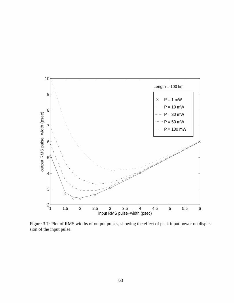
P = 1 mW

P = 10 mW

P = 30 mW

P = 50 mW

P = 100 mW

1 1.5 2 2.5 3 3.5 4 4.5 5 5.5 62

3

4

5

6

7

8

9

10

input RMS pulse−width (psec)

ou

tpu

t R

MS

pu

lse

−w

idth

(p

sec)

Length = 100 km

Figure 3.7: Plot of RMS widths of output pulses, showing the effect of peak input power on disper-sion of the input pulse.

63

increases, the optimum input pulse-width increases. For a peak pulse power of��

mW, the mini-

mum output pulse-width of about � psec is achieved at a input pulse-width of about � psec. For very

low power levels, output pulse-widths as low as � psec can be achieved.

We now study the pulse-to-pulse interactions due to fiber nonlinearities in systems that use co-

herent light by calculating signal-to-interference ratios (SIR). We study the effect of pulse-width,

symbol period and peak pulse power on the signal-to-interference ratios (at the detector) due to

linear dispersion, interaction between linear dispersion and fiber nonlinearities, and nonlinear inter-

action exclusively due to fiber nonlinearities.

The output intensity is calculated as the magnitude squared of the received field� �� , the

inverse-Fourier transform of� - � � � in (3.5). There are three terms in the expression for output

intensity, (i) the linear-linear interaction term, that includes the signal, the inter-symbol interfer-

ence, and nonlinear interference due to the square-law detector, (ii) the linear-nonlinear interaction

term, and (iii) nonlinear-nonlinear interaction term that includes the self-phase modulation (SPM),

cross-phase modulation (CPM), and four-wave mixing (FWM) components. The signal energy is

calculated by integrating the linear component over the symbol period of interest. The interference

energy is calculated over six adjacent symbol periods on either side of the symbol of interest. In

our simulations, we found the linear-nonlinear interaction term to be negligible (on the order of SIR

�� dB) compared to the other two terms. The nonlinear-nonlinear interaction term consists of the

interaction of the pulse with itself and interaction of the pulse with other pulses through the highly

coherent light used. The interaction of the pulse with itself is mainly due to self-phase modulation

and does not depend upon the symbol period used; as we increase the symbol period, all other terms

decrease almost exponentially.

Figure 3.8 shows how the SIR at the detector varies with symbol period for different peak pulse

powers. As the symbol period increases, the SIR due to dispersion increases steadily. However, the

SIR due to nonlinearities does not increase much above a symbol period of� �

psec.

Figure 3.9 shows how the SIR at the detector varies with peak pulse power for different symbol

64

SIR due to linear dispersion

SIR due to fiber nonlinearities

total SIR

0 0.5 1 1.5 2 2.5 3 3.5 4 4.5 50

10

20

30

40

50

60

70

80

90

100

power (mW)

10

lo

g(s

ign

al−

to−

inte

rfe

ren

ce

ra

tio

)

T = 3 psec

z = 100 km

−−− Ts = 10 psec

−o− Ts = 30 psec

Figure 3.8: Output SIR as a function of symbol period for different power levels.

65

SIR due to linear dispersion

SIR due to fiber nonlinearities

total SIR

5 10 15 20 25 30−20

0

20

40

60

80

100

symbol period (psec)

10

log

(sig

na

l−to

−in

terf

ere

nce

ra

tio)

T = 3 psec

z = 100 km

−o− P = 2 mW

−−− P = 5 mW

Figure 3.9: Output SIR as a function of peak pulse power for different symbol periods.

66

periods. We can see that the SIR due to dispersion increases enormously with the symbol period;

however, the SIR due to nonlinearities is limited by the peak pulse power. For large symbol periods

and moderate input powers, the SIR is limited by the fiber nonlinearities.

3.4 Summarized Observations

A frequency-domain Volterra Series Transfer Function (VSTF) description for the nonlinear

Schroedinger (NLS) wave equation is derived and it is shown that for most communications ap-

plications, even a third-order approximation to this model can predict the nonlinear behavior of

single-mode optical fiber remarkably well. The third-order approximation to the model is suffi-

cient for powers that the current semiconductor lasers can generate for communication applications

(� � � � mW) and for reasonable lengths of fiber (

� � �� km); for higher power levels, the accuracy

of the model can be increased by taking into account higher-order Volterra kernels. We have demon-

strated this by using a fifth-order VSTF method and showing that the performance is as accurate as

the split-step Fourier (SSF) method for all power levels and fiber lengths of practical interest. The

analytical method presented here is more accurate than the SSF method for long lengths and smaller

pulse-widths. The existence of an analytical model can also provide insight into the effects of non-

linearities and possible ways of removing the detrimental effects. We have provided the dispersion

and nonlinear parameters required to design an equalizer. The interference caused by a pump pulse

on the signal pulse is presented as a function of frequency difference between their central frequen-

cies. The Raman effect is shown to be smaller and less important for all frequency separations for the

parameters used here. Lastly, the output SIR for a simple communication system is given to show an

example of how the VSTF method can be used to analyze and design better optical communication

systems.

67

Chapter 4

Linear Dispersion in Fiber-opticCommunications

Before we study the effect of fiber nonlinearities on a communication system, we evaluate the effect

of linear dispersion alone. Since the phase noise of the source determines the extent of dispersion, it

is important that we include it [9, 74, 10]. The coherence time introduces a phase relation between

the field at different times and when this signal is incident on a photo-detector, this phase relation

manifests as a nonlinear interaction between pulses generating nonlinear interference. In addition,

these phase variations are converted into amplitude variations (PM-to-AM conversion [6]), adding

what we call intensity noise. We evaluate and optimize the fiber optic communication system using

the signal-to-interference ratio (SIR) as a measure of performance.

The presence of phase noise or lack of source coherence makes the dispersion effects more

severe and changes the pulse shape considerably. On the other hand, coherent light (no phase noise)

suffers most from signal-dependent nonlinear interference introduced due to the nonlinearity of the

photo-detector. The intensity (amplitude) noise generated by phase noise is found to be a maximum

for completely incoherent light (has white spectrum), while being zero for coherent light.

68

4.1 Derivation of SIR for Arbitrary Light Source

We derive the first two moments of the output of the photo-detector for the general case of partially

coherent light and then specialize the results to the cases of completely coherent light and completely

incoherent light. If we denote the impulse response of a fiber for the optical field by�� , i.e., the

inverse-Fourier transform of�� - � � � in (2.19), then

� ��

�� (4.1)

where we have not showed the explicit dependence of�� on the length of the fiber � . The ex-

pectation of the the (random) instantaneous intensity of the optical field� �� that is incident on

the detector when we apply a random optical field with complex envelope� �� at the transmitting

end of the fiber is given by

� � � ��

��

� �� (4.2)

Recalling (2.1), the three random processes affecting the signal are phase noise ) �� , the random

pulse phase ' )'� ( �� , and the data stream ' & ��( �� . The first and second moments of the intensity

over just the phase noise are given by

� � � �� "$� � � ��

��

� �� $ � � � � $ �� (4.3)

and

� � � �� #"$� � � ��

��

��

� ��

��

� ��

�� $ � � � � $ �� $ �� $ � �� (4.4)

Using the fact that ) �� is a Wiener-Levy process, i.e., a Gaussian process with zero mean and

correlation function � � ) ��) � � �� , we can easily show that the mean is

� � � �� "$� � � ��

��

� �� &�� ' $ � � $ � ' � � � � � � � (4.5)

69

and the covariance function given �� is

� � �� ' � ��,� � ��

��

��

� ��

��

� ��

�� &�� $ � � $ � � $ � � $ � � � � �&� �� ' $ � � $ � ' � ' $ � � $ � ' � � � � � � � � � � � � � (4.6)

where � � � �� #� � � � � � � � �!� , where �!� �� are � � �� arranged in increasing

order.

Since � �� in (2.1) is completely described by ' ) � � & ��( �� , we obtain

� � � �� ' )� � & � ( �� & � � ��

��

�� & � & � �� (4.7)

where we have used & �� & � . The first term

� ��

��

� �� &� � � ' $ � � $ � ' � � � �� (4.8)

represents the linear component which includes the signal component and the usual inter-symbol

interference (ISI) due to linear dispersion effects. The second term

� �'��

��

� �� &�� ' $ � � $ � ' � � � �� (4.9)

represents the nonlinear interference (crosstalk) term which includes interference due to the nonlin-

earity of the detector. Recall ) � is the random phase associated with the � th pulse due to timing

jitter. From (4.6), the intensity noise given the jitter and information bits is

� �� ' )� � & � ( ��

�� &� ��

�� ,� ��

�� & � � & � � & � � & � � � � � � � � � ��

� �! � �� (4.10)

where

� �!��

��

��

� ��

��

� ��

� � � � � � � � � � � � � � � � � � � � �&�� $ � � $ � � $ � � $ � � � � �&� � � ' $ � � $ � ' � ' $ � � $ � ' � � � � � � � � � � � � � (4.11)

70

Knowing these Volterra kernels � � �� , � �'� �� , and � � �� , we can (i) optimize the de-

sign, decide on necessary coherence time, pulse-width and symbol period for a given length of fiber

and given a decoder algorithm, (ii) calculate a realistic performance of the existing algorithms, and

(iii) design inverse Volterra kernels necessary to compensate for these effects thus improving the

decoding algorithms. We address (i) and (ii) in Section 4.2 and leave the latter for Chapter 6.

The expected value in (4.7) is still stochastic because of the phase term � � � � � �* � , the phase

difference between different pulses. The expectation of the intensity with respect to ) � , given the

data is given by

� � � �� ' & ��( �� & � � � � �� (4.12)

The variance or noise introduced due to this phase difference is

� �� ' )� � & � ( �� ' & ��( ��

�� & � & � � �'�� (4.13)

This is the nonlinear noise that appears as the variance of the intensity. This term is shown to be

zero for incoherent light and maximum for coherent light in the next sections.

Using the independent and identically distributed nature of pulse phases, taking the expectation

of (4.10) with respect to the pulse phase, we are left with the terms with ' � � � � � � � � � � � ( and

' � � � � � � � � � � � ( , which give us the mean intensity noise in presence of timing jitter as

� � � � � � � �� ' )� � & � ( �� ' & � ( ��

� � � ��

� �� & � � & � �

� �! � � � � � ��

�� & � � �! � � � � � �� (4.14)

We show the effect of phase noise on the linear dispersion by using the signal-to-interference

ratios (SIR) at the detector for a theoretical optical source that can generate pulses of any width

and coherence time. We define the SIR as the ratio of signal energy to interference energy within a

symbol period. Assuming ' &��( �� to be equally likely and independently distributed, taking the

expectation with respect to ' & � ( �� , the expected signal energy in the interval� � �� for bit &�� in

71

(4.7) is

Signal ��

� � " $� � �� (4.15)

The expected energy due to dispersion in the interval� � �� in (4.7) is

Dispersion �

�

�

� � ��

" $ � �� (4.16)

The expected energy due to nonlinear interference in the interval� � �� in absence of jitter in (4.7)

is

Nonlinear interference ��

��

� �� (4.17)

The expected energy due to nonlinear noise (i.e., with jitter) in the interval� � �� in (4.13) is

Nonlinear noise ��

� � ��

�� '�� (4.18)

The expected energy due to intensity noise in the interval� � �� in (4.10) (without the jitter) is

Intensity noise ��

� � �

� � � ��

� � � ��

� � � �� ! �� (4.19)

The expected energy due to intensity noise with jitter in the interval� � �� in (4.14) is

Intensity noise ��

�

�� ! �� (4.20)

4.1.1 Completely Coherent Light

For completely coherent light, using � � � �in (4.5) and (4.6), we obtain the first two moments as

� � � �� " � � � ��

��

� �� (4.21)

and� � �� ' � ��

, i.e., the covariance function in absence of phase noise is, of course, zero.

Therefore, the expected intensity noise� � � � � �� ' ) � � & ��( ��

.

Substituting � � � �in (4.8) and (4.9) yields

� � ��

��

� �� (4.22)

72

� �'� ��

��

� �� (4.23)

The expected intensity in (4.7) was derived for completely coherent light in [21] with no timing

jitter.

4.1.2 Completely Incoherent Light

For completely incoherent light, taking the limit as � �� " in (4.5) yields

� � � �� #" � � � ��

��

� ��

� � �� (4.24)

We notice that this is a linear convolution of the intensity of the input with the magnitude square

of the impulse response of the fiber to the optical field. For intensity-modulated communica-

tion systems using incoherent light, the input intensity can be written as� ��

� �� & � � �� , where� �� is the intensity of the pulse shape, and &�� are again the infor-

mation bits. This gives us

� � � �� ' & � ( �� & � �

�� (4.25)

We can conclude that the impulse response of the fiber to the optical field is completely different

from the impulse response of the fiber to the intensity, as shown in [21, eq. (12)]. The nonlinear

interference (crosstalk) has disappeared as there is no phase relation between any points for incoher-

ent light, thus the detector nonlinearity does not add nonlinear interference. In the presence of jitter,

the nonlinear noise term does not appear either.

In the limit as � �� " , we see that (4.11) gives us

� �!��

��

��

� ��

��

� ��

� � � � � � � � � � � � � � � ��

� � � � � � � � � � � � � �� (4.26)

73

where� �� is the magnitude of the input pulse,

��

� �!� � � � � �� where

� � �� !� � are � � �� arranged in increasing order. However, �� only if

�!� � � and � �� . Therefore, the intensity noise in (4.14) does not vanish for incoherent light.

4.2 Numerical Results

We assume that the laser generates a Gaussian pulse shape with intensity given by (3.15) with � �

�mW and

�� . In this work, numerical results for two different fibers of different lengths are

presented. First, a GVD dominant case, i.e.,�� psec

�/km, and

��

�with a fiber length

of � � � km is considered. Second, operation at the zero-dispersion wavelength, i.e.,��

�, and�

� ��

psec�/km with a fiber of � � � km, is then analyzed. The length of � � � km for third-order

dispersion dominant case has been chosen to represent a practical situation, within the so called

“dispersion limit” [75] for the given data rate, and the length of � � � km for the GVD dominant case

has been chosen to make the performance of both cases comparable.

Figure 4.1 shows the output intensity pulse shapes when a pulse of width�

psec having different

coherence times is injected into the two fibers under consideration. These plots show that the level of

coherence has a strong effect on the output pulse shapes. For a GVD dominant fiber of length � � � km,

we can see from Figure 4.1(a) that the pulse shape is Gaussian for coherent light ( �� psec).

The pulse shape is non-Gaussian for partially coherent light ( � � �psec), and the dispersion is

over approximately � � pulse-widths. For the almost incoherent case ( � ��

psec), we can

see that the pulse shape is very non-Gaussian and the dispersion is approximately over � � pulse-

widths. The pulse shape is almost square, with more signal energy in the adjacent slots than the

slot in which the pulse was transmitted. The reason signal coherence has such a strong effect on

dispersion is that as light becomes more incoherent, the bandwidth of the channel described by the

fiber with the coherence function decreases below that of the bandwidth of the impulse response

without coherence function (for coherent light), thus spreading the signal more than the dispersion

74

input pulse

coherence time = 0.005 psec

coherence time = 5 psec


−25 −20 −15 −10 −5 0 5 10 15 20 250

1

2

3

4

5

x 10−4

time/rms pulsewidth

inte

nsity

Length = 2.2 km

(a)

input pulse




−4 −2 0 2 4 6 8 10 12 14 160

0.1

0.2

0.3

0.4

0.5

0.6

0.7

0.8

0.9

1x 10

−3

time/rms pulsewidth

inte

nsity

Length = 320 km

(b)

Figure 4.1: Output pulse shapes for different levels of coherence of light for input pulses of�

psecRMS width: (a) GVD dominant case (b) operation at zero-dispersion wavelength, � � .

75

alone would have. We need to understand here that pulse-widths of�

psec can not currently be

generated with incoherent sources having coherence times as small as� � � � �

psec. This waveform is

of theoretical interest only.

As seen in Figure 4.1(b), for operation at the zero-dispersion wavelength with a fiber length of

� � � km, the effect of dispersion is very small for coherent light. For the partially coherent case,

dispersion has increased considerably (over 10 pulse-widths) compared to coherent light, and the

dispersion is even more for almost incoherent light, extending over 15 pulse-widths. Tails become

quite heavy for incoherent light. The energy is transferred into the future bits only and previously

transmitted bits are not affected.

We now illustrate the dispersion as a function of source coherence. We use the RMS pulse-

width for a single pulse � �� given by (3.20) as a measure of the effects of dispersion. We have

plotted in Figure 4.2 the output RMS pulse-width versus input RMS pulse-width, for various values

of coherence time for the two cases under consideration. We can see that as the coherence time

decreases (light becomes more incoherent), dispersion increases, increasing the output pulse-width.

For coherence time smaller than� � �

psec, we do not see much change in output RMS pulse-width

from those obtained for� � �

psec. Note that pulses below�

psec for the GVD dominant case ( � psec

for operation at zero-dispersion wavelength) experience extreme dispersion, even for coherent light.

Sending pulses of width shorter than�

psec can result in much wider received pulses than if wider

pulses had been transmitted as observed in [3, 28]. The smallest output RMS pulse-width even with

the most coherent light source is obtained when the input pulse is�

psec for the GVD dominant

case and � psec for operation at the zero-dispersion wavelength. Therefore, compared to the GVD

dominant case, we can afford to use smaller pulses for operation at � � . Depending on the coherence

time, the pulse-width for which pulses with minimum width are received changes for the same fiber

length.

This shows that shortening the input pulses even with more coherent light sources may not give

shorter output pulses. As we see in the next section, in addition to not necessarily getting shorter

76

coherence time < 0.1 psec




0 5 10 15 20 25 30 35 40 45 500

10

20

30

40

50

60

70

80

90

100

input pulsewidth (psec)

outp

ut p

ulse

wid

th (

psec

)

Length = 2.2 km

(a)

coherence time < 0.1 psec




0 5 10 15 20 25 30 35 40 45 500

10

20

30

40

50

60

70

80

90

100

input pulsewidth (psec)

outp

ut p

ulse

wid

th (

psec

)

Length = 320 km

(b)

Figure 4.2: Plot of RMS pulse-widths of output pulses, showing the effect of coherence time ondispersion: (a) GVD dominant case (b) operation at zero-dispersion wavelength, �� .

77

output pulses, nonlinear interference is added to the output when we use coherent sources.

4.2.1 Communication System Performance

So far we have seen the effect of source coherence on the shape of the single pulse obtained at the

output of the photo-detector and looked at the RMS pulse-width of a single pulse for different input

pulse-widths and different coherence times.

Now we analyze the performance of a communication system transmitting a pulse stream op-

erating with fixed input pulse-width and symbol duration. We have plotted the shapes of the total

received signal and the nonlinear interference from (4.7) showing the effect of pulse separation in

Figure 4.3. For the GVD dominant case (Figure 4.3(a)) and less coherent light, the dispersion (as an-

ticipated) spreads the pulse so severely that we can not distinguish two adjacent pulses; the nonlinear

interference also shows the same spreading but with smaller amplitude. When the coherence time is

larger than the input RMS pulse-width ( �� psec), the spreading is less severe and the width of

the nonlinear interference is also small but the amplitude of the nonlinear interference is much larger

compared to less coherent light. When we double the pulse separation, the nonlinear interference

decreases drastically for less coherent light, but makes less of a difference for coherent light. This is

because of increased interaction between pulses due to larger coherence times compared to symbol

periods.

For operation at the zero-dispersion wavelength (Figure 4.3(b)), since dispersion is into future

bits only, the effect of dispersion is smaller, but nonlinear interference is much larger for less co-

herent light. We observe more oscillations in the intensity, due to faster variation in phase for

third-order dispersion. For coherent light, since dispersion is very small, pulses do not overlap thus

produce little nonlinear interference compared to the GVD dominant case.

Now we look at quantitative measures of performance of communication systems. Our perfor-

mance measure is the signal-to-interference ratio (SIR) due to dispersion, nonlinear interference and

intensity noise. Our goal is to determine numerically the optimal input pulse-width for which max-

78

−100 0 1000

0.2

0.4

0.6

0.8

1

x 10−3

inten

sity

Ts = 30 psec

−100 0 1000

1

2

3

4

5

6

x 10−4

−100 0 1000

0.5

1

1.5

x 10−6

−100 0 1000

0.2

0.4

0.6

0.8

1

x 10−3

time (in psec)

inten

sity

Ts = 60 psec

−100 0 1000

1

2

3

4

5

6

x 10−4

time (in psec)−100 0 100

0

0.5

1

1.5

2

2.5

x 10−15

time (in psec)

−100 0 1000

0.2

0.4

0.6

0.8

1

x 10−3

−100 0 1000

1

2

3

4

5

6x 10

−5

−100 0 1000

0.2

0.4

0.6

0.8

1

x 10−3


0

0.2

0.4

0.6

0.8

1

1.2x 10

−6

time (in psec)

Input Nonlinear noise Received Nonlinear noiseReceived

cct = 1 psec t = 128 psec

(a)

−50 0 500

0.2

0.4

0.6

0.8

1

x 10−3

inten

sity

Ts = 30 psec

−50 0 500

1

2

3

4

5

6

x 10−4

−50 0 500

0.2

0.4

0.6

0.8

1x 10

−5

−50 0 500

0.2

0.4

0.6

0.8

1

x 10−3

time (in psec)

inten

sity

Ts = 60 psec

−50 0 500

0.2

0.4

0.6

0.8

1

x 10−3


0.2

0.4

0.6

0.8

1

x 10−14

time (in psec)

−50 0 500

0.2

0.4

0.6

0.8

1

x 10−3

−50 0 500

0.2

0.4

0.6

0.8

1

1.2x 10

−5

−50 0 500

0.2

0.4

0.6

0.8

1

x 10−3


1

2

3

4

5

6

x 10−7

time (in psec)

c ct t= 1 psec = 128 psec

ReceivedInput Nonlinear Noise Received Nonlinear Noise

(b)Figure 4.3: Plots of different waveforms of expected received signal (signal and mean nonlinearinterference) and �� showing the effect of pulse separation on the nonlinear interference:(a) GVD dominant case (b) operation at zero-dispersion wavelength.

79

imum SIR is obtained for a given coherence time and data rate. To this end, we have defined six

parameters. The signal-to-interference ratio (SIR) due to dispersion is the ratio of the expected sig-

nal energy in the integration interval of interest to the mean square interference caused by dispersion,

(using (4.15) and (4.16)),

� �� " $� � ��

�� "%$ � �� (4.27)

The SIR due to nonlinear interference is the ratio of the expected signal energy in the integration

interval of interest to the mean square nonlinear interference of (4.17),

� �� "%$� � ��

�

��

� �� '� �� (4.28)

The SIR due to nonlinear noise (in the presence of jitter) is the ratio of the expected signal energy in

the integration interval of interest to the mean nonlinear noise of (4.18),

� �� "%$� � ��

�

�� (4.29)

The total SIR due to dispersion and nonlinear interference is the ratio of the expected signal energy

in the integration interval of interest to the energy due to dispersion of (4.16) and the mean square

nonlinear interference of (4.17),

� �� $ �� " $� � ��

�� " $ � ��

��

� �� '� �� (4.30)

The SIR (defined similarly) due to intensity noise introduced by the phase noise in absence of jitter,

given in (4.19) is

� �� " $� � ��

� ��

� � � �� ! �� % �� (4.31)

Lastly, the SIR due to intensity noise introduced by the phase noise in presence of jitter given in

(4.20) is

� �� "%$� � ��

�� (4.32)

80

For computational reasons, we integrate the interference caused over ten adjacent symbols, five on

either side of the symbol of interest. This is consistent with the largest fiber dispersion and coherence

time considered. In our simulations, we found that taking ten such symbols is accurate within an

error of��

, in the worst case.

Figure 4.4 shows the six SIR measures as the source coherence varies. The system is assumed to

use an input RMS pulse-width of�

psec with a symbol period of � � psec. As light becomes more and

more coherent, dispersion decreases, and nonlinear interference increases. The SIR � for incoherent

light is smaller than�

dB. For incoherent light, nonlinear interference is very small, and as light be-

comes more and more coherent, (and dispersion decreases) nonlinear interference increases rapidly,

then as the coherence time exceeds the pulse-width (i.e., when � �� ), interaction between

pulses does not change too much, and nonlinear interference changes very little with increasing co-

herence time. SIR �� is slightly smaller than SIR �� for smaller coherence times. We have indicated

the asymptotes by using�

’s, wherever the SIR’s are finite. The asymptotes calculated using the

formulae in Sections 4.1.1 and 4.1.2 conform quite well with the curves calculated for partially co-

herent light, confirming the limiting behavior of the light for completely coherent and completely

incoherent light. For completely incoherent light, the intensity noise is considerably smaller than the

interference due to dispersion and considerably larger than nonlinear interference or noise. How-

ever, as light becomes more coherent, the intensity noise decreases and becomes much smaller than

both the interference due to dispersion and nonlinear interference or noise. The intensity noise is

maximum for the completely incoherent case and is only of theoretical interest, as we can not gen-

erate pulses with pulse-widths as small as�

psec with very short coherence times. Timing jitter

increases intensity noise considerably. For operation at the zero-dispersion wavelength � � , Figure

4.4 (b) show the same trend as the GVD dominant case, except that the SIR � ’s are considerably

higher and the SIR �� or SIR �� remains fairly constant across values of �� .Figure 4.5 shows the dependence of SIR � and SIR �� on coherence time for a pulse-width of

�psec and for different symbol periods. The SIR �� is more affected by the increasing symbol period

81

SIR due to dispersion SIR due to nonlinear interference total SIR without jitter SIR due to nonlinear noise SIR due to intensity noise SIR due to intensity noise with jitter

−1 −0.5 0 0.5 1 1.5

0

10

20

30

40

50

60

70

log(coherence time/pulsewidth)

10 lo

g(si

gnal

−to

−in

terf

eren

ce r

atio

)

Length = 2.2 km

(a)

SIR due to dispersion

SIR due to nonlinear interference

total SIR without jitter

SIR due to nonlinear noise

SIR due to intensity noise

SIR due to intensity noise with jitter

−1 −0.5 0 0.5 1 1.50

10

20

30

40

50

60

70


10 lo

g(si

gnal

−to−

inte

rfer

ence

rat

io)

Length = 320 km

(b)

Figure 4.4: Plot of SIR � , SIR �� , SIR �� , SIR � , and SIR � � showing the effect of coherence timeand timing jitter for a fixed symbol period of � � psec and a pulse-width of

�psec,

�’s indicate the

asymptotic values, � � �and �! � " , calculated from formulae in Sections 4.1.1 and 4.1.2: (a)

GVD dominant case, (b) operation at zero-dispersion wavelength, �� .82

symbol period = 30 psecsymbol period = 40 psecsymbol period = 50 psec

−1 −0.5 0 0.5 1 1.5−20

0

20

40

60

80

100

120

140


10 lo

g(si

gnal

−to−

inte

rfere

nce

ratio

)

Length = 2.2 km

(a)

symbol period = 30 psec



0 0.5 1 1.50

10

20

30

40

50

60

70

80

90

100


10 lo

g(si

gnal

−to−

inte

rfere

nce

ratio

)

Length = 320 km

(b)

Figure 4.5: Plot of SIR � (shown with ’o’s), and SIR �� , showing the effect of coherence time foran input RMS pulse-width of

�psec and different symbol periods for (a) GVD dominant case (b)

operation at zero-dispersion wavelength.

83

than the SIR � . Since the separation between pulses increases with increasing the symbol period,

nonlinear interaction between pulses decreases thus giving smaller values for nonlinear interference.

For smaller symbol periods, the symbol overlap makes the SIR �� exceed the SIR � even for �! � � as

low as�. The coherence time at which nonlinear interference exceeds the dispersion increases with

increasing symbol periods. For operation at the zero-dispersion wavelength, the behavior is similar

but with larger SIR’s and relatively higher nonlinear interference as compared to dispersion.

Figure 4.6 shows the variation with input pulse-width of the SIR � , SIR �� and SIR $ for differ-

ent coherence times for the GVD dominant case. Our aim is to determine the pulse-width for

which maximum SIR is achieved, and whether such optimal pulse-width depends on the coherence

time. From Figure 4.6(a), we see that the nonlinear interference increases drastically with increasing

pulse-width for less coherent light. As light becomes more and more coherent, the nonlinear inter-

ference increases and its dependence on pulse-width decreases. For less coherent light, pulse-width

makes very little difference for SIR � ; however, as light becomes more coherent dispersion decreases

and its dependence on input pulse-width increases. The maximum SIR � is achieved for a � � � psec

input pulse-width for all coherence times. Note that this is different from that predicted by disper-

sion alone in Figure 4.2. Here we are considering the effects of inter-symbol interference and not

simply RMS pulse-width. The pulse-width for which maximum SIR �� is achieved seems to increase

slightly with coherence time. This effect cannot be used in practice since to generate short pulses

we require highly coherent sources.

Figure 4.6(b) shows that the SIR $ changes with pulse-width for different coherence times, reach-

ing a maximum for coherent light when pulse-widths are large. As pulse-width decreases below

� psec, partially coherent light seems to do better than the coherent light.

Figure 4.7(a) shows the variation of optimum input RMS pulse-width (input pulse-width for

which maximum SIR is achieved) as we vary the coherence time for different symbol periods. As

the symbol period increases, the choice of coherence time increases the optimum pulse-width dras-

tically, and the optimum pulse-width depends more and more on coherence time. For smaller coher-

84





2 3 4 5 6 7 8 9 100

5

10

15

20

25

30

35

40

45

50

rms pulsewidth (psec)

10 lo

g(si

gnal

−to−

inte

rfere

nce

ratio

)

Length = 2.2 km

(a)





2 3 4 5 6 7 8 9 100

2

4

6

8

10

12

14

16

18

20

rms pulsewidth (psec)

10 lo

g(si

gnal

−to−

inte

rfere

nce

ratio

)

Length = 2.2 km

(b)

Figure 4.6: Plot of the (a) SIR � (shown with ‘o’s) and SIR �� , and (b) SIR $ showing the effect ofcoherence time for a symbol period of � � psec for different pulse-widths for a GVD dominant case.

85






0 0.5 1 1.5 2 2.54

4.5

5

5.5

6

6.5

7

7.5

8

8.5

9

log(coherence time (in psec))

optim

al in

put r

ms

puls

ewid

th

Length = 2.2 km

(a)






0 0.5 1 1.5 2 2.50

5

10

15

20

25

30

35

40

45

log(coherence time (in psec))

10 lo

g(m

axim

um s

igna

l−to

−int

erfe

renc

e ra

tio)

Length = 2.2 km

(b)

Figure 4.7: Plot of the (a) optimal input pulse-widths and (b) SIR $ ’s for optimal pulse-width fordifferent symbol periods for a GVD dominant case.

86

ence times, dispersion dominates, therefore the optimal pulse-width is larger (dispersion is smaller

for larger pulse-widths); for larger coherence times, nonlinear interference dominates and the pulse

overlap has to be reduced, thus we need to use larger pulses (to reduce dispersion). Figure 4.7 (b)

shows that all SIR’s for optimal pulse-widths show almost the same behavior, increasing with coher-

ence times initially, then increasing rapidly, and then remaining almost constant for larger coherence

times. For smaller symbol periods, we see a decrease in SIR for large pulse-widths, and from the

trend we can conclude that for a given symbol period, we can find an optimum coherence time

and pulse-width for which SIR achieves a maximum. The SIR’s of course increase with increasing

symbol period.

4.3 Summarized Observations

Volterra kernels describing the effect of phase noise on the intensity of the light received at the

photo-detector are derived. The effect of coherence time on dispersion, the addition of nonlinear

interference/noise and intensity noise are presented. It is shown that lack of source coherence intro-

duces a phenomenal increase in dispersive effects in fiber-optic systems using direct-detection. The

pulse shapes are quite different for incoherent light as compared to coherent light. Low coherence

increases the dispersive effects drastically making the pulses indistinguishable from adjacent pulses

making the decoding at the receiver impossible. However, high coherence introduces excessive non-

linear interference which can become comparable or sometimes even stronger than the interference

due to dispersion even for moderately small coherence times � � �� . The second moment of the

received intensity gives rise to what we call “intensity noise”, which can become considerable for

smaller coherence times. Timing jitter can cause a measurable increase in the nonlinear interference

and intensity noise.

We conclude that the use of smaller input pulse-widths does not necessarily mean better perfor-

mance. There is an optimal input pulse-width for which the output pulse-width is minimum; there

87

is also an optimal input pulse-width (possibly different) for which the SIR is maximum, and such

optimal input pulse-widths depend on the choice of coherence time. As we develop highly coherent

ultrashort pulses, we are introducing nonlinear interference/noise, with almost no reduction in the

RMS pulse-widths of pulses received or increase in the SIR at the receiver.

This work provides tools to choose an optimal input pulse-width for a given source coherence

time and symbol period (data rate). The Volterra kernels derived here can also be used to design

filters either in the optical domain or the electronic domain to reduce the nonlinear interference/noise

and intensity noise.

88

Chapter 5

System Design

A new methodology for designing fiber amplifier based optical communication systems is presented

in this chapter. We derive the overall Volterra series transfer function of the system including linear

dispersion, fiber nonlinearities, amplified spontaneous emission (ASE) noise from the fiber ampli-

fiers, and the square-law nature of the direct detection (DD) system. Since analytical expressions for

the probability of error are difficult to derive for the complex systems being used, we derive analyti-

cal expressions for an upper bound on probability of error for integrate-and-threshold detection at the

receiver. Using this bound as a performance criterion, we determine the optimal dispersion param-

eters of the fiber segments required to minimize the effects of linear dispersion, fiber nonlinearities

and ASE noise from the amplifiers. We study the dependence of optimal dispersion parameters on

the average power levels in the fiber by varying the peak input power levels and the amplifier gains.

Analytical expressions give us the freedom to choose system parameters in a practical manner, while

providing optimum system performance. Using a simple system as an example, we demonstrate the

power of the Volterra series approach in designing optimal optical communication systems. The

analysis and the design procedure presented in this work can be extended to the design of more

complex wavelength division multiplexed (WDM) systems.

In Chapter 3, we proposed a VSTF approach for modeling the interaction of linear dispersion

and fiber nonlinearities in an optical fiber. We showed that the Volterra series approach can pro-

vide an accurate description of the effects of linear dispersion and fiber nonlinearities. For practical

89

power levels (on the order of�

mW), we showed that a third-order approximation to the VSTF yields

results comparable to the split-step Fourier method. In addition to providing an accurate descrip-

tion of the behavior of an optical fiber, the VSTF also provides an analytical tool to design modern

systems. In this chapter, we offer an example of the potential of this analytical method to design

complex optical fiber systems. We determine the overall VSTF of a fiber system including fiber

and amplifier parameters in an analytical form. Using an approximation of this transfer function,

we determine optimal dispersion parameters to minimize linear dispersion, fiber nonlinearities, and

ASE noise. These approximations can be removed depending on the accuracy required at the cost of

additional computations. The optimality criterion desired is the probability of error for which ana-

lytical expressions are difficult to derive due to the complex nonlinear receiver statistics. Therefore,

we use an analytical upper bound on the probability of error, namely the modified Chernoff bound,

as a performance criterion. The derivation of this bound depends on analytical expressions for the

output optical field provided by the VSTF method.

The most logical performance measure in the design of digital optical communication systems

is the probability of error. Unfortunately, analytical expressions for the probability of error are in-

tractable. Even though the Volterra series approach provides an analytical expression for the optical

field incident on the photo-detector, the probabilistic models used in the current literature for the

photo-detection process are inadequate for modeling practical situations. Therefore, we determine

bounds on error probability at the receiver, and then determine the optimal dispersion parameters

that minimize this bound.

In Section 5.1, we present the optical communication system model used in this chapter and

derive the overall VSTF. In Section 5.2, we derive the statistics of the received optical field. We

introduce the modified Chernoff bound in Section 5.3 and derive the required moment generating

function (MGF) of the output current from the photo-detector including linear dispersion, fiber non-

linearities, the behavior of the amplifiers and thermal and shot noise processes at the receiver. The

use of these analytical expressions in system design is demonstrated on a very simple system in Sec-

90

tion 5.4. Optimal system parameters that minimize the probability of error for this simple system

are determined, illustrating how our method could be used for more complex system design. The

dependence of the optimal dispersion parameters on power levels in the fiber are demonstrated by

varying the input peak power and amplifier gains.

5.1 Transfer Function of the System

Currently most optical communication system design methods rely on analytical expressions avail-

able for single-pulse propagation [20, 46, 66]; however, the design is verified using a stream of

pulses, and fine tuning of the system parameters is done heuristically [51, 52, 56]. In this work, we

start with multi-pulse propagation and design the system including multiple pulse interactions. The

complex envelope of the input field is given by

� � ��

�� & � � �� (5.1)

where � is the peak power of the input pulse, & � ' � � � ( are the transmitted bits, � ��

� � �� is the basic pulse shape used to transmit the � th bit, and � � is the symbol period.

There has been a few attempts to optimize the performance of amplified based optical communi-

cation systems. The problem of determining the optimum location of the amplifier (when only one

amplifier is used) in a link was considered by Fellegara [66]; however, linear dispersion and fiber

nonlinearities, which play a dominant role in determining the amount of interference and noise at

the receiver, were ignored. In this chapter, we compare the relative performance of different kinds

of amplifier chains used in practice, including the effects of linear dispersion, fiber nonlinearities,

and ASE noise. We assume a system with � sections of fiber with Erbium doped fiber amplifiers

(EDFAs) placed between each section as shown in Figure 5.1. We consider four different amplifier

chains mentioned in Section 2.2.4 and shown in Figure 5.1, namely, Type A, B, C, and AC amplifier

chains. We first derive the transfer function of a general system which we then use to derive the

transfer functions of the different configurations in Figure 5.1. A block diagram representation of

91

Receiver

� � � ��

� � ��

� � ��

� � ��80 km 80 km 80 km 80 km

Laser EDFAEDFA EDFA EDFA

(a) Type A amplifier chain

� � ��

� � � ��

� � ��

� � �� 64 km 64 km 64 km 64 km 64 km

Laser ReceiverEDFAEDFA EDFA EDFA

(b) Type B amplifier chain

106 km 106 km 107 km� � �Receiver

� � ��

� � � ��

� � ��

� � ��Laser EDFAEDFA EDFA EDFA

(c) Type AC amplifier chain

� � � ��

� � � ��

� � ��

� � ��Laser EDFAEDFA EDFA EDFA Receiver

80 km 80 km 80 km 80 km

(d) Type C amplifier chain

Figure 5.1: Typical communication systems used to demonstrate the design procedure.

92

� ��

� �� - �

� � ��

� � ��

� � ��

� � �� - � � � - �

Figure 5.2: Block Diagram of the cascade of % th fiber amplifier and % th fiber segment.

the cascade of one amplifier and one fiber segment is shown in Figure 5.2 for the % th fiber amplifier

and % th fiber segment.

For low input power levels, the fiber amplifier can be modeled as a linear filter� � � - � ��

� � � - � , where � � � - � is the frequency dependent gain of the % th amplifier in the amplifier chain.

The ASE noise from the % th amplifier, �� , can be assumed to be circularly symmetric complex

Gaussian distributed with power spectral density � � � - � � �� - � � �

�� W/Hz, where �

is the optical frequency of operation,�

is Planck’s constant, and � �� is the spontaneous emission

parameter, which is a measure of the degree of inversion achieved in the amplifier [27].

We define� � - � as the Fourier transform of the complex envelope

� � �� of the input to the

% � � � th fiber segment (the input field to the first segment is� � �� , defined in (5.1)). The transfer

function of the % th fiber segment of length � � can be written as

� � - � � � � �� - � � � �� - �� - � (5.2)

where� � �� - � � � �

��

� � � ��

��

(5.3)

is the linear transfer function and the second term in (5.2) accounts for the third order fiber nonlinear-

ity. The function � � �� - � is the linear fiber kernel where � � � and

� � ��

�� are the attenuation

and dispersion constants of the fiber segment, respectively, � is the center wavelength used,�

is the

speed of light, and � is the usual dispersion used in current optical communication literature. In the

above model, we have ignored the effect of the third-order dispersion (dispersion slope), as its effect

is negligible for lengths much smaller than� � � � � � km.

93

The nonlinear functional � � �� - � is defined as

� �� - � � � � � � �� - � ��- � ��- � - � ��- � � � - � � � � - � � � - � - � ��- � � � - � � - � � (5.4)

where the third-order Volterra kernel is given by (3.10), for which we are using the approximation,

� � �� - � ��- � ��- � � � �� #� � � �� ,� � � ��

�� - � � - � � - � � - � � � �'�� '� � ��

(5.5)

where �� is the effective length of the % th fiber segment. The approximation to

� � �� in (5.5) includes only terms linear in

� � �� ; in our simulations, we included up to cubic terms,

omitted from (5.5) for brevity. The approximation in (5.5) also neglects the effects of higher-order

nonlinear coefficients, � � , � � , and � � .The expression in (5.2) is a third-order approximation to the VSTF of the optical fiber. The

approximation error incurred in ignoring the higher-order Volterra kernels can be easily shown to

be order��

� � �� , where �

� �� is the nonlinear length associated with the SPM

constant � � �� of the % th fiber segment, and � is the peak output power of the laser. Since this term is

about� � ��

of the power contributed by the linear term of the output field for typical power levels of�

mW, we can safely ignore the higher-order kernels. In certain cases when the system parameters

used result in high power levels in the fiber, we may have to include fifth order kernels as discussed

in Chapter 3.

As shown in Chapter 3, the Volterra series model provides an analytical description of the inter-

action of linear dispersion and fiber nonlinearities in a single segment of optical fiber. When two

systems are cascaded, we obtain an equivalent Volterra expansion for the combined system in terms

of the VSTFs of the two sub-systems. The order of nonlinearity of the concatenated system is the

sum of the orders of nonlinearities of the sub-systems. In our case, we ignore the higher-order terms

introduced by cascading the subsystems and use only the third-order approximation of the VSTF of

the overall system.

When we include the linear transfer function and ASE noise of the fiber amplifiers, (5.2) yields

94

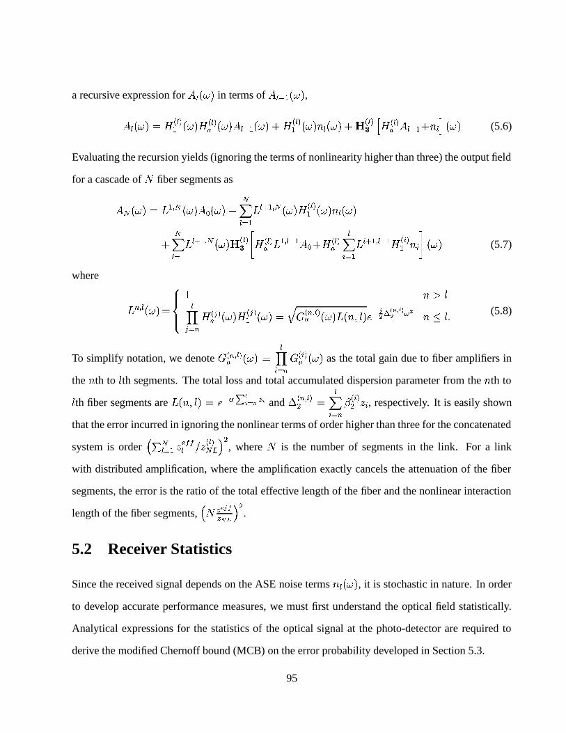
a recursive expression for� � - � in terms of

� � �� - � ,� �� - � � � � �

� - � � � � - � � � �� - �� - �� - �� - � (5.6)

Evaluating the recursion yields (ignoring the terms of nonlinearity higher than three) the output field

for a cascade of � fiber segments as

� � - � �� - � � �' - � � ��

� � � � � - � � � �� - �� - �

��

� � � � � - � � �� !� � �

�!� � � � �� - � (5.7)

where

� � � � - � �� %��

� �� - � � �� - � �

�� - �� %��

�� % � (5.8)

To simplify notation, we denote � � � � � - � ��!� � �

�!� - � as the total gain due to fiber amplifiers in

the � th to % th segments. The total loss and total accumulated dispersion parameter from the � th to

% th fiber segments are � � � %�� and � � � � �

� �

��!� �

� �!�� , respectively. It is easily shown

that the error incurred in ignoring the nonlinear terms of order higher than three for the concatenated

system is order��

� � �� , where � is the number of segments in the link. For a link

with distributed amplification, where the amplification exactly cancels the attenuation of the fiber

segments, the error is the ratio of the total effective length of the fiber and the nonlinear interaction

length of the fiber segments,� � � �� .

5.2 Receiver Statistics

Since the received signal depends on the ASE noise terms � �� - � , it is stochastic in nature. In order

to develop accurate performance measures, we must first understand the optical field statistically.

Analytical expressions for the statistics of the optical signal at the photo-detector are required to

derive the modified Chernoff bound (MCB) on the error probability developed in Section 5.3.

95

From (5.7), the output field� � �� at the end of � sections (incident on the photo-detector) is a

Gaussian process with mean,

� ��

�� & � � � ��

� � � � � �

��

�%� ��

� � �� & � &� & � � � � � � � �� (5.9)

and covariance function

� � ��

� � ��

��

� � � - � � � � � � �� - � � � � � � - �� ,�� $ � � � � - � � � � � � �� (5.10)

where the nonlinear terms of order greater than three have been ignored in the mean and all nonlinear

terms are ignored in the expression for covariance.

Volterra kernels are expressed in the frequency domain, whereas the field statistics are best ex-

pressed in the time-domain. Therefore, we provide expressions for various terms in the output field

in the frequency domain, then take the Fourier transform to get the expressions in the time-domain.

In all cases we use the argument - � or �� to denote the frequency or time domain, respectively.

The linear part of the output field in the frequency domain at the receiver due to the � th input

pulse is

� �� - � � � � � � - �� - � � � �

� � � �'� � � � � � � � � � (5.11)

and the nonlinear interaction of different pulses is given by

� � � � � � �� - � �

��

� � � � � - � � � � � �� - � ��- � ��- � - � � - � �� - � �� - � �� - � - � � - � �

� �� - � �� #� � - � �� - � - � � - � �� - � � - � � � �� '� � � � � � � � � � (5.12)

where � � � - � � � � � - �� - � . The nonlinear interaction between the information signal and

the ASE noise is included via the noise kernels, given by

�� - � ��

� � � � � - � �� - �� - � � � � � � � � �

� � � � ��- � �� (5.13)

96

�� - � �

��

� � � � � - � � � � �� - � � � �� - � �� (5.14)

where

�� - � � � � � - � � � � � �� - �� - � � (5.15)

�� - � � � � � � - � � � ��%� � � � �#� � � � �� - �� #�

� - � � � � �#� - � (5.16)

�� - � � � � � � - �� #� �

� � �#� � � � �� - �� #�� - �� #� - � (5.17)

are the linearly filtered signal and the filtered power spectral density of the noise at the % th fiber

segment. Notice that the noise term �� - � in (5.13) corresponds to the CPM from the ASE noise

used in current literature and the noise term�� - � corresponds to the FWM between the signal

and the ASE noise. We can evaluate� �� - � and �� - � accurately, whereas for analytical ease,

we use a third-order approximation of� � � � � � �� - � and

�� - � , i.e., all terms and cross-products of� � �

� ��% � � � � � � � � � � , of powers higher than three are ignored.

In practice, four-wave mixing (FWM) between the ASE noise and the signal is said to introduce

modulation instability (MI). Typically, in the derivation of the parametric gain due to modulation

instability [20], only the cross-phase term due to the intensity of the noise term is included. From

(5.13) and (5.14), we can see that in our case only the cross-phase modulation (CPM) term con-

tributes to the mean of the output signal. The FWM term should appear in the covariance of the

output signal; however, we have ignored that term as it is expected to be negligible compared to

the variance of the ASE noise. We would have to include FWM in the covariance term to see how

the modulation instability theory available in the literature fits our model. Nevertheless, the mean

of the output signal contains two signal-ASE interference terms given by (5.13) and (5.14), which

shows that the choice of dispersion parameters does affect the nonlinear interaction of signal and

ASE noise, and consequently the noise statistics at the receiver.

97

5.3 Modified Chernoff Bound (MCB)

The current methods of analysis do not provide analytical closed-form performance expressions

suitable for system optimization. They are typically based on simplified models, and system pa-

rameters are varied in a heuristic fashion to get the best performance from the system [56, 51, 52].

To design better systems, analytical methods for studying the combined effects of dispersion, fiber

nonlinearities, MI, ASE noise, and the detector (square-law) nonlinearities are required.

We use the MCB [54, 76] as a measure of performance of the communication system. The

Chernoff bound (CB) provides a tight upper bound for the probability of error useful when the

computation of the probability of error is not tractable. This bound takes into account the shot

noise, thermal noise, and other interference terms due to linear dispersion and fiber nonlinearities.

In addition, due to the inclusion of the ASE noise, the beat terms between the ASE noise and signal

are implicitly included in the MGF description. The modified Chernoff bound (MCB) is tighter

than Chernoff bound when the system has significant thermal noise. For a��

Gbps systems, thermal

noise is significant due to the requirement for small rise times at the receiver, so the MCB provides

a tighter bound than the CB.

Ribeiro et. al. [54] have advocated the use of tight bounds on the probability of error. The MGF

of the output current was derived, and used to evaluate the performance of an EDFA pre-amplified

receiver. The mean and variance of the Gaussian approximation were derived and were shown to

be the same as those derived from semi-classical analysis [27, 66, 46]. The effect of thermal noise,

the photo-detector response, and ISI was included in the description of the error bounds. The error

bounds such as Chernoff bounds and saddle-point approximation were shown to be tighter than the

Gaussian approximation, i.e., receiver�

. However, the derivation in [54] indirectly appeals to the

central limit theorem (which implicitly means deriving the Gaussian model). Moreover, by initially

assuming that the observation interval is greater than the reciprocal of the optical bandwidth and

allowing it to tend to zero, the model assumes an infinite optical bandwidth, which is not very

98

practical. In this chapter, we derive a more accurate MGF for the output current at the photo-

detector, including the spectral distribution of the ASE noise, which provides a more realistic bound

on the probability of error. The MGF derived in this chapter takes into account the effect of linear

dispersion and fiber nonlinearities on the spectral distribution of ASE noise and takes into account

the effect of finite optical bandwidth at the receiver (either due to intentional filtering or photo-

detector response characteristics).

We assume direct-detection with integrate-and-threshold detector to be used for extracting the

information from the received signal, with no additional electronic signal processing. The decision

statistic, � is the current produced by the optical signal� � �� integrated over the time interval� �� . Without loss of generality, we consider detecting bit & � &'� , i.e., the bit transmitted

over the time interval of interest � � �� . The MCB is given by [76]

� � � � � ��

�� $��

� � �� $�� ' � � � �� ' � � � �

�� (5.18)

where � �$�� is the variance of the thermal noise and� ' � � � is the MGF of the decision statistic when

& is the bit transmitted in the interval of interest.

To derive the expressions for� ' � � � for &�� , we expand the received optical signal using

a Karhunen-Loeve series [21, 54]. This allows us to derive statistics of each of the terms in the

series and thereby obtain the MGF of the output current at the receiver. For � � much greater than

the width of the covariance function� � � � , i.e., for large bandwidth noise spectrum and for large

optical bandwidth compared to the data rate, the eigenfunctions of the Karhunen-Loeve expansion

of the incident signal are complex exponentials [21]

� �! ��

� � �� ,� � $ � - � � ��

��

(5.19)

and the corresponding eigenvalues are given by

� � � � � - � � ��

� � � - � � � � � � � �� - � � � � � � � - � � (5.20)

99

Typically � � is the symbol period of interest and the width of� � � � is smaller than � � due to the

large amplifier bandwidth and large optical bandwidth used at the receivers.

We find the MGF given the transmitted symbols, & � ' &�� ( , and & � &�� , using

the method of conditioning [21], which gives

�� ' � � � � � � � ��!� �

� � � � � � ��

� � � � � � � (5.21)

where� � � � � � � � � � � . The responsivity of the photo-detector is given by � � �� , where

�is

the quantum efficiency of the detector,�

is Planck’s constant, � is the optical frequency at which the

signal is being transmitted, and � �� "%$�� , where � is the optical bandwidth at the receiver. The

signal eigenvalues are

� � ��

�� " $ � �� " $ � � � �� $ � � � &

� � �� !�

� � � �!�� !�

� � � � � � � � � � � � �!�

� ��

�� & �

� � �� !�

� � � � � �!�� !�

� � � � � � � � � � � � �!�

� �

� & � �,��

�� & �� (5.22)

where � � � ��

�" $ � "%$��

� "%$�� $ � � corresponds to the linear portion of the output field for bit

& � , and similarly � � � � �� !��

�"%$ � " $ ��

� " $ � � � � � � � � �� ,� � $ � � corresponds to nonlinear portion of the out-

put field due the interaction between pulses &�� , &� , and & � . � � � � �� and

� � � �!�� are similarly defined.

Typically, the nonlinear interaction of a pulse with itself dominates all other contributions from the

nonlinear interaction between three different pulses; therefore, we have assumed in (5.22) that only

� � � � � � �!��

� � � �� contributes to the output field. Notice that we do get beat terms

between different pulses due to the squaring operation; however, this is a property of the photo-

detection process, rather than the behavior of the fiber. Now taking the expectation with respect to

& , yields

� ' � � � �� !� �

�

� � � � � � �

��

�� & ��!� �

� �,��

� ��

100

��

�

�

��

��

�� & ��!� �

� � � ��

� ��

��

� � � � � ��

� �� (5.23)

where� �,�� ,�� is the

�th eigenvalue of the signal energy received due to the pulse corre-

sponding to bit & � & � in the interval� �� , � � � ��

� � � � �,�� and� � � � � ��

� � � � �� represent the ISI due to the both linear dispersion and fiber nonlinearities.

5.4 Design Example

We demonstrate the design procedure to optimize the MCB for a simple system. More complex

systems can be designed easily as an extension to the analysis in this section.

The optimization can be carried out to get optimal parameters of any component in the system. In

this section, we concentrate on determining the optimal dispersion parameters� � �� % � � � � � � � � �(�

of the fiber segments. Such optimum dispersion parameters can be obtained by solving the system

of nonlinear equations, � � � � � � � �� (5.24)� � � � � � � � �

��

� � % � � � � � � � � � � �(5.25)

Substituting the MGF into the MCB and in (5.24) and (5.25), analytical expressions can be obtained

and the MCB can be numerically minimized. introduced in Section 2.2.4 and determine the relative

advantages of different configurations in reducing fiber nonlinearities and ASE noise at the receiver.

To keep the presentation simple, we make the following assumptions:

1. We use the input pulse shape � �� shown in Figure 5.3.

2. All segment lengths and amplifier gains in a given configuration are equal for a total link

length of � � � km. Exactly four amplifiers are used in each case. All amplifier configurations

use a receiver with the same sensitivity.

101

−200 −150 −100 −50 0 50 100 150 2000

0.01

0.02

0.03

0.04

0.05

0.06

0.07

0.08

0.09

0.1

Time in psec.

Pow

er in

mW

Figure 5.3: Input pulse shape used. The input pulse corresponding to & � is shown with a solid lineto stress that this is the bit of interest.

102

3. The amplifier gains are independent of frequency. The ASE noise spectrum is white within

the optical amplifier bandwidth as well as the optical bandwidth at the receiver, so that we can

use � � � � � � � - �� % � � � � � � � � . For simplicity, we assume that the gains of the amplifiers

are equal i.e., � � � � � � � % . Therefore,

� � � � � � � � � ��

� � � � �� (5.26)

is independent of�. The coupling losses to the fiber amplifier are assumed to be absorbed in

the amplifier gain, and the gain given by � should be understood as the total amplifier gain

less the coupling losses.

4. The saturation properties of the fiber amplifiers are ignored, i.e., it is assumed that the amplifier

gains can be varied without saturation. In most cases in the numerical results presented, the

input power is lower than the typical input saturation powers of � �dBm; therefore, except for

very high amplifier gains, the results should be accurate.

5. Typically in manufacturing fibers, dispersion parameters are tailored by varying the effective

cross-sectional area of the fiber. Therefore, the attenuation constant � � and nonlinearity pa-

rameter � � also change accordingly, which can be accounted for in the model. In this study,

for simplicity, we ignore this dependence, and assume that the attenuation constant and non-

linearity parameter do not depend on the dispersion.

We assume the symbol rate to be� � � ��

Gbps, i.e., the symbol period is��

psec. For the integrate-

and-threshold receiver assumed, the optical bandwidth is � ��

GHz for � � � . We

assume the electrical bandwidth to be at least twice the symbol rate (as per the Nyquist criterion) of

�� GHz. The load resistance

� � is determined by the rise time of the detector, which

is��

� � � � � � , with the capacitance of the photo-diode at�

pF, giving a thermal noise variance of

� �$�� " � � ��

A�, where � is the temperature in Kelvin.

103

We assume that some parameters, like attenuation, third-order dispersion (dispersion slope),

and nonlinear coefficient � � are fixed and equal for all fiber segments. In this chapter, we use

� �� dB/km, giving an effective length � �� km, and � � � �

/W-km, giving a nonlinear

interaction length � � � of about� � �

km for an input power level of�

mW. As already noted, we

assume the dispersion slope to be zero.

Figures 5.4 (a)-(d) show plots of the MCB as a function of the total equivalent span gain for

different peak input powers for the different configurations shown in Figure 5.1 (a)-(d), respectively,

using optimal dispersion parameters. For low amplifier gains, the performance improves propor-

tional to the amplifier gains due to the increase in received power levels compared to the thermal

noise at the receiver. In contrast, for large amplifier gains, the performance degrades considerably

more rapidly than the improvement in the performance seen at lower power levels. This is due to the

fact that the increase in received power is proportional to the amplifier gain, whereas the degradation

in performance due to fiber nonlinearities is proportional to the cube of the amplifier gain. There

is an additional degradation in performance at higher amplifier gains due to the accumulated ASE

noise at the receiver. As expected, lower peak input powers require higher gain to achieve optimal

performance compared to the higher input power levels in all plots. The received power level is

almost identical for the optimal amplifier gain for the three input levels used; the only difference in

the optimal performance is caused by the differing ASE noise.

Figure 5.4 (a) shows that for a Type A system, the system performance is determined primarily

by fiber nonlinearities. For low power levels, the performance is almost the same for all peak input

powers. The best performance is achieved when the received power is about � � dBm, which con-

firms previous analytical [77] and experimental [78] results stating that if the power levels are below�

dBm, the nonlinearities do not affect the system. When we use low peak input power levels, the

optimal system performance is considerably better than when the peak input power levels are high.

The Type C amplifier chain in Figure 5.4 (c) has behavior completely opposite to the Type A

system; the higher peak input powers provide better performance than the lower input peak powers.

104

−10 −5 0 5 10 15 20 25 3010

−18

10−16

10−14

10−12

10−10

10−8

10−6

10−4

10−2

100

Total span gain − Total span loss (dB)

Mod

ified

Che

rnof

f Bou

nd

P = −16 dBm P = −13 dBm P = −10 dBm

−10 −5 0 5 10 15 20 25 3010

−18

10−16

10−14

10−12

10−10

10−8

10−6

10−4

10−2

100


Mod

ified

Che

rnof

f Bou

nd

P = −16 dBm P = −13 dBm P = −10 dBm

(a) (b)

−10 −5 0 5 10 15 20 25 3010

−18

10−16

10−14

10−12

10−10

10−8

10−6

10−4

10−2

100


Mod

ified

Che

rnof

f Bou

nd

P = −16 dBm P = −13 dBm P = −10 dBm

−10 −5 0 5 10 15 20 25 3010

−18

10−16

10−14

10−12

10−10

10−8

10−6

10−4

10−2

100


Mod

ified

Che

rnof

f Bou

nd

P = −16 dBm P = −13 dBm P = −10 dBm

Total span gain - Total span loss (dB)

(c) (d)

Figure 5.4: Upper bound on the probability of error using the optimal dispersion map for differentconfigurations shown in Figure 5.1 as a function of amplifier gain for different input powers � .

105

This seems to indicate that the system is not dominated by fiber nonlinearities, which is as expected

since the power levels are lower due to the absence of a booster amplifier.For low amplifier gains,

the higher power levels obviously provide better performance and for high amplifier gains, the lower

power levels provide better performance, which is expected as the fiber nonlinearities are less in that

case. The performance at higher amplifier gains is almost the same as that for a Type A system. The

best performance is obtained for a Type C system for high peak input power levels, for a received

power level of � �dBm, which indicates that this system is ASE noise dependent.

The Type B amplifier chain performance in Figure 5.4 (b) shows that the performance is in

between that of the Type A and the Type C amplifier chains, which is expected. The system is

determined by both fiber nonlinearities and ASE noise. The plots are more symmetrical and the

best system performance is obtained for higher input peak powers and lower amplifier gains. The

received power for the best performance is about � � dBm.

Figure 5.4 (d) shows very interesting results for a Type AC system. The fiber segment lengths

for the Type AC are much longer; therefore, fiber nonlinearities are not a big problem as attenuation

reduces the signal levels to a very small values. However, the amount of improvement provided

by using optimal dispersion parameters may not be as significant, since the degrees of freedom is

small (three). The optimal performance seems to be very close for all the input peak power levels,

except that the optimal amplifier gains are obviously different. Therefore, the received power for the

optimal performance is almost the same for all the input power levels. We note that the lower input

peak power levels seem to perform slightly better than the higher input peak power levels. There is

an interesting behavior seen for medium power levels ( � � � dBm). The performance improvement

with amplifier gain reaches an optimum value, and starts degrading with increasing amplifier gains

(due to the fiber nonlinearities); however, it levels off before increasing again. Further analysis is

required before the cause of this odd behavior can be explained, or to see if it is possible to take

advantage of this behavior.

Figure 5.5 shows the total accumulated dispersion as a function of distance from the transmitter,

106

0 100 200 300−1000

−500

0

500

1000

distance from the transmitter (km)

Tot

al d

ispe

rsio

n pa

ram

eter

(ps

ec2 )

P = −16 dBm P = −13 dBm P = −10 dBm

0 100 200 300

−1200

−1000

−800

−600

−400

−200

0


Tot

al d

ispe

rsio

n pa

ram

eter

(ps

ec2 )

P = −16 dBm P = −13 dBm P = −10 dBm

0 100 200 300−500

−400

−300

−200

−100

0


Tot

al d

ispe

rsio

n pa

ram

eter

(ps

ec2 )

P = −16 dBm P = −13 dBm P = −10 dBm

0 100 200 300

−800

−600

−400

−200

0


Tot

al d

ispe

rsio

n pa

ram

eter

(ps

ec2 )

P = −16 dBm P = −13 dBm P = −10 dBm

Figure 5.5: The optimal total accumulated dispersion parameter determined by minimizing the MCBfor different configurations shown in Figure 5.1 and for different input powers. The lines indicatedispersion parameters for amplifier gains close to the optimal amplifier gains and the ’ � ’ indicatedispersion parameters for amplifier gains higher by

�� dB per amplifier than the optimal amplifier

gains.

107

for different input power levels and for amplifier gains close to the optimum and gains slightly higher

than the optimal, for the four configurations shown in Figure 5.1. For the Type A system shown in

Figure 5.5 (a), the dispersion parameters for low input peak power levels and low amplifier gains are

negative (dispersion � is positive) in the initial segments, and is positive (dispersion � is negative)

in the later segments; the overall accumulated dispersion increases on average with power levels and

amplifier gains. However, for the largest input peak power levels and largest amplifier gains, the

optimal dispersion map is similar to the equi-modular dispersion compensation [60], which seem

to suggest that for a Type A system, for high input peak powers and for high amplifier gains, equi-

modular dispersion compensation is optimal.

For a Type C system shown in Figure 5.5 (c), the accumulated dispersion maps are similar to

those of the Type A system; however, the total dispersion parameter is always increasing with the

input peak power. The dispersion parameters increase steadily also with amplifier gains. Optimal

dispersion maps for a Type B amplifier are similar to the Type C, except that the total accumulated

dispersion parameter is close to zero, with the small total dispersion parameters increasing steadily

with amplifier gains. The most unexpected behavior is seen from the Type AC amplifier chain in

Figure 5.5 (d). The system is no longer attempting to maintain the total accumulated dispersion

parameter close to zero, allowing it to increase significantly with both the input peak power as well

as the amplifier gains. Further analysis of the analytical expressions is required before a thorough

study of the optimality of these dispersion maps can be made.

5.5 Concluding Remarks

We have presented a new methodology for designing fiber amplifier based optical communication

systems using the Volterra series transfer function (VSTF) of the fiber. A closed-form expression for

the output field of the overall system in terms of the input field and fiber and amplifier parameters

is derived. Using this expression for the output field, closed-form expressions for the modified

108

Chernoff bound on the probability of error are derived. The availability of a closed-form expression

for a bound on the probability of error allows minimization of this bound to obtain optimal system

parameters.

We have used the VSTF approach to design a relatively simple optical communication system to

demonstrate the power of the approach. We have determined the optimal dispersion parameters for

different input peak power levels and amplifier gains for different configurations used in long-haul

optical communication systems. The analysis shows that a reasonably low error probability can be

achieved by choosing dispersion parameters optimally and choosing the input peak power levels

and amplifier gains appropriately. The comparison used is the standard equi-modular compensation

used in current optical communication systems. We show that an optical communication system

using a Type A amplifier chain is dominated by fiber nonlinearities (so low input peak powers with

high amplifier gains are better), whereas a Type C system is dominated by ASE noise (so high input

peak powers with low amplifier gains should be preferred). For a Type B system, the behavior is

somewhat in between the Type A and Type C system as expected. We observe that Type C and

AC chains can achieve lower error probabilities than the Type A and B chains. We also observe

an advantage of more than one order of magnitude in using the optimal dispersion map over the

equi-modular map for some cases. This illustrates the benefits possible by optimizing system design

using our method.

More accurate analyses with less approximations are required before the results can be vali-

dated (especially by including the higher order Volterra kernels for higher input peak power levels

and higher amplifier gains). The same analysis and system design can be easily extended to more

complex wavelength division multiplexed (WDM) systems.

109

Chapter 6

Conclusions and Future Work

In this chapter we discuss the conclusions that can be made from this work about the analysis and

design of fiber-optic communication system in the presence of linear dispersion and fiber nonlinear-

ities using the Volterra series transfer function (VSTF) approach. We then discuss possible future

work concentrating more on the design of wavelength division multiplexed (WDM) systems and

improving the tools developed in the previous chapters.

6.1 Summary

Analytical expressions can be very useful in the analysis and design of future high bandwidth optical

communication systems. Due to the increased accuracy provided by analytical results, it is possible

to include all the deleterious effects in an optical communication system. The design of the system

is therefore better than possible with currently available simple models and recursive (numerical)

solutions to the wave equation in the fiber. The performance measures used to design and evaluate

current systems, such as SONET standards based on eye-diagrams, should be re-evaluated and more

stringent and realistic measures should be defined.

We present one candidate analytical method based on the Volterra series transfer function

(VSTF) that gives very good insight into the shortcomings of the analysis and design tools used

in current systems. A third-order approximation to the VSTF is accurate enough without being

110

computationally intensive, and provides improvements over the current models in most cases. How-

ever, further development of this method or newer methods are necessary before the full potential of

the analytical methods can be exploited. We have presented the modified Chernoff bound (MCB) as

a possible candidate for defining the performance of an optical communication systems, which can

include all the deleterious effects such as linear dispersion, fiber nonlinearities, and ASE noise from

the optical amplifiers.

We have presented a general method of deriving various kernels in the VSTF of a SMF. We have

demonstrated the accuracy of a third-order approximation to the VSTF by comparing the results

with those the of SSF method. We have shown that for higher power levels, higher-order kernels are

required to be included to give comparable results to the SSF method. We have demonstrated the

potential of the VSTF approach by designing a complex fiber-optic link including fiber amplifiers

and by designing an optimal lumped equalizer. We have shown the accuracy of the VSTF approach

in modeling multi-frequency propagation in the fiber. We have determined the optimal input param-

eters (pulse-width, power, and coherence time) required to get a minimum output RMS pulse-width

and maximum optical signal-to-interference ratio (SIR).

We have investigated the effect of phase noise on high speed optical communication systems

including only the linear dispersion effects. We have shown that the effects of phase noise can not

be analyzed properly by including its effect on the source line-width only. The previous studies

based on line-width use only the mean and variance of the input field, whereas we include mean

and covariance of the input field. Although, we do not obtain analytical results for the effects of

phase noise, this more accurate analysis provides insight into the incorrect assumptions made in the

current analysis and provides a strong platform to perform further analysis.

We have demonstrated the power of the VSTF approach in modeling the propagation of light in

the fiber by designing a simple optical communication system. Fixing all the other parameters in the

system, we determine the optimal dispersion parameters of the fiber segments used in the system.

We study the improvement provided by using the optimal dispersion parameters, and study the effect

111

of the choice of input power levels and amplifier gains on the optimum dispersion parameters and

the probability of error. We also study the relative merits of different amplifier chains used in current

systems.

Now we consider the most important application of the VSTF method, where it can have the

most impact, namely wavelength division multiplexed (WDM) systems. Then we consider a few

topics of further work to be done to utilize the advantages provided by the VSTF approach.

6.2 Future Work

Most high throughput communication systems use WDM to increase he capacity. The effects of

fiber nonlinearity are more pronounced in WDM systems than in single-user systems since the total

power is higher and the frequency content is broader. As a part of future work we show in Appendix

A how the VSTF can model the three nonlinear Kerr effects observed in WDM systems. The ana-

lytical expressions are found to be the same as the most accurate analysis available in the literature.

Therefore, we can conclude that modeling of WDM systems can also be carried out with the same

accuracy as the single-user communication systems. There are many aspects of WDM that can be

considered in system design, such as the number of channels, wavelength assignment, user powers,

and pulsewidths. The VSTF can be a powerful tool is the optimal design of such systems.

The Volterra kernel model used in this work has been derived using many significant assump-

tions and is presented to show the validity of the approach. For higher power levels, higher-order

Volterra kernels are necessary which make the VSTF approach impractical. Therefore, better non-

linear models that are more representative of the fiber nonlinearities (e.g., phase-only effects) in an

optical fiber are required. Even though the value of the availability of analytical expressions has

been stressed in this dissertation, there is no analysis of various phenomena presented and how the

VSTF approach can model the nonlinear phenomena in an optical fiber better is not shown. A fuller

analysis of various effects in the fiber is required to gain more understanding of the design and anal-

112

ysis of optical communication systems. More specifically, we have to find a symmetrized version

(with respect to the arguments to the kernels) of the VSTF presented in Chapter 3, which will make

it invariant to the order of inputs and the arguments of the Volterra kernels [79, 80]. The convergence

properties of the VSTF as a function of power levels, lengths of fibers, and pulse-width have to be

quantified to determine when it is necessary to include higher-order Volterra kernels.

The split-step Fourier (SSF) approach is not a valid method for modeling bi-directional systems

[81]; the SSF method requires knowledge of signals propagating in both directions in each segment

to calculate the evolution of the fields in the fiber. Recursively running the SSF method through the

length of the fiber calculating the field in one direction while using the signals for the other direction

from previous iterations is one approach of analyzing the performance, but the requirement to store

the field for each segment length for the whole fiber and the computational cost make it impractical.

Since the VSTF approach provides a closed-form solution, it can model the behavior of the bi-

directional systems as a simple extension of the model presented in Chapter 3.

The fiber amplifier is modeled as a linear filter in this work. A nonlinear (possibly Volterra

series) model to describe the behavior of the amplifier including the saturation properties [27] and

inter-modulation distortion [82] between various channels in a multi-user system is required. The

saturation induced cross-talk is due to the dependence of the carrier or ion concentration in the

gain medium of the amplifier on the input intensity. More sophisticated models based on the VSTF

method can be derived as an easy extension of the work presented in this dissertation. Currently

the threshold at the receiver is varied based on the receiver�

, in an ad-hoc fashion as a function

of median received signal levels to reduce the effects of saturation induced cross-talk, which is not

optimal. The VSTF can describe the behavior of the amplifier in saturation, or at least a statistical

description of the EDFA behavior in saturation based in VSTF can easily be derived for current

power levels used in terrestrial systems. Inter-modulation distortion is significant only when the

wavelengths are so closely spaced that the ion density can respond only at the beat frequency.

Polarization mode dispersion (PMD) [23, 83, 84] is significant in optical communication systems

113

longer than��

km. We have to include the PMD effects in the Volterra series to better model the

behavior of the optical communication system. Wai and Menyuk have formulated the problem of

analyzing PMD as solving a stochastic differential equation in the frequency domain in [23]. We

have solved the deterministic NLS equation using VSTF method in this dissertation, and it is a

straight-forward extension to solve the stochastic NLS equation using the Ito operator used also in

[23].

We have shown that WDM systems can be modeled easily with the VSTF method including all

the major effects observed in experiments. The effect of dispersion slope on the WDM systems can

be easily accommodated in the Volterra series approach and the dispersion slopes can be tailored to

get the required dispersion maps to assure that the probability of error for all the users is the same

and is a minimum. From the results in Chapter 5, it is not clear how the dispersion maps that are

optimum for single-user systems work for multi-user systems like WDM systems. Further analysis

based on Appendix A is required to understand the behavior of the system.

The Volterra series model used in this work can be used to study the transmission of solitons in a

fiber-optic medium. Since analytical expressions are available, we can find the stochastic properties

of the output pulse such as timing jitter, amplitude jitter, etc. [22] and choose the fiber to suit the

soliton-propagation and thus improve the performance of soliton systems.

The Volterra series method is a general method of solving the NLS equation, and therefore it can

be used to model coherent optical systems, especially dense WDM systems [49]. The expressions for

coherent systems are simpler as they depend only upon the output field rather than output intensity

(direct-detection). However, the effect of phase noise of both the input laser and the local oscillator

has to be included in the output statistics, which makes the analysis using the results from Chapter

3 and 4 more useful.

Using the already available Volterra series models for the semiconductor laser nonlinearities

[4, 5], we can develop more accurate analytical expressions for the output field in analog optical

communication systems [7]. Since the requirements of analog communications are more severe

114

and fiber nonlinearities and dispersion can at best be perturbations, the third-order approximation to

the Volterra model is more suitable for use in analog systems, making the analysis and design very

simple.

We have assumed a photo-detector with ideal impulse response, which is not very realistic. It

is quite straight-forward to include the photo-detector response in the moment generating functions

(MGF) [21], and derive more realistic upper bound on the probability of error following the analysis

in Chapter 5.

We have considered only point-to-point optical fiber links in this work. Due to the increasing de-

mand for more bandwidth, optical networks are becoming more and more complex. Minimizing the

probability of error for the whole network is of interest, and the true capability of the VSTF method

can be exploited to optimize the system performance for all users and channels in the network.

With the increasing accuracy of current tapped delay lines, optical signal processing is becoming

more and more popular for incoherent light. Nonlinear coherent couplers have been suggested

[20, 72, 73] to perform the basic switching and basic processing in the optical domain. The VSTF

model is an universal tool that can even include these complex components in the analysis and design

of systems.

We would like to conclude this dissertation with the hope that the basic theory presented in this

dissertation will stimulate further work improving the VSTF design tools and applying it to future

high capacity photonic networks, thus making system design more science than art.

115

Appendix A

Analysis of WDM Systems Using VSTFmethod

Although the VSTF method is equally valid for analyzing TDM and CDM systems, we concentrate

on WDM systems in this appendix. In a WDM system, the wavelength or frequency of the optical

carrier is used to multiplex the signals from various users. These signals are extracted from the

composite signal using wavelength selective switches. Typical wavelength spacings are � � � GHz

for WDM systems and��

GHz for dense WDM (OFDM) systems.

In addition to all the factors considered for single-user systems, there are a few additional factors

that should be taken into account for the WDM systems due to the presence of signal at various

frequencies, e.g., the effect of the group velocity�� and the dispersion (frequency-dependence) of

the nonlinear refractive index � � - � . Since pulses at different wavelengths propagate at different

speeds inside the fiber, because of the group-velocity mismatch, the faster moving pulse “walks

through” the slower moving pulses. The walk-off parameter is the fiber length over which one pulse

”walks through” another slow moving pulse. In a typical WDM system, a fast moving pulse can

walk through about��

pulses in a long haul network, thus introducing nonlinearities that extend

over thousands of pulses.

In single-user communications, for pulse-widths greater than about� � �

psec, the dispersion

116

(frequency-dependence) of the nonlinear refractive index � � - � can be ignored�. However, when

multiple users are present, frequency dependence of the the Kerr effects and Raman effects has to

be included. When using the split-step Fourier method, the dispersion (frequency-dependence) of

Raman effects are included in the frequency-domain and the Kerr effects are included in the time-

domain, which makes switching between the time- and frequency-domains necessary [38]. With the

availability of the Volterra kernel method, the frequency dependence of these nonlinear effects can

be included.

The dispersion (frequency-dependence) of the nonlinear part of the refractive index is assumed

to be a perturbation of the overall refractive index. This assumption is valid if the intensities we are

considering are small. If we assume transmission at multiple frequencies/wavelengths at practical

power levels ( � � mW), we need to include the frequency dependence of � � - � and we can include

� � - � as shown in [58].

Now we consider various phenomena observed in WDM systems, and see how well the VSTF

models them. For a WDM system, the complex envelope of the input field is the sum of complex en-

velopes (about a common central frequency) of the signals from�

users with the � th user operating

at a wavelength of - � ,� � ��

��

�� ,� � $ �

��

��

�� & � �� ,� � $ (A.1)

where � � is the peak power of the input pulse of the � th user, & � �� are the transmitted bits of user � ,

� �� is the basic pulse shape used by all users to transmit the � th bit, and � is the

delay of � th user relative to user�.

Let us examine the linear and nonlinear parts of the mean output field given by (5.9) for the input

(A.1) separately. Writing � - � � � � - � � � �'�� - � , the Fourier transform of the linear part is a�For pulse widths �� psec, the electronic contribution to the third-order susceptibility �� occurs at a time scale

of �� fsec in optical fibers.

117

sum of the filtered outputs of different users,

� � - � � � � � � - � ��

��

�� & � �� - � - � � � (A.2)

It contains ISI components of a single user due to adjacent bits transmitted by the same user and

any possible signal from adjacent users due to improper optical filtering at the receiver. The Fourier

transform of the nonlinear part contains various terms that represent self-phase modulation (SPM),

cross-phase modulation (CPM), and four-wave mixing (FWM) terms, without ASE noise,

� �� - � ��

� � � � � - � � �� - �

�

��

� � � � � - � � � � � �� - � ��- � ��- � - � ��- � �

��

��

�� *� �

��

��

��

� � �� - � � � � �

�� - � � � � �

� - � - � ��- � �� - � � � � � � �� - � �� - � - � ��- � �� - � � - � � � � � ��

� - � � - � � � � � �,�� - � - � ��- � � - � � � � - � � - � (A.3)

We now see how the VSTF model can predict the four-wave mixing products. We can get

expressions for SPM and CPM by taking the appropriate terms from the FWM expression. While

modeling the FWM in optical fibers, different wavelengths are assumed to be sinusoids, which in

the frequency domain are impulse functions. Therefore, assuming� � - � � � - � , we get

� �� - � � ��

� � � � � - � � � � �� - � � ��- � � ��- � � �

��

��

�� &� �

��

��

��

� � �� - � � � � � �

�� - � ��

� - � � � � � � � �� - � � � � � � � �� - � � �� - � � � (A.4)

for - � � - � � � - � � ��- � � . From (3.10), we get the third-order Volterra kernel as

� � �� - � � ��- � � ��- � � � � ��

� �� - � � � � � � � - � � � � � � � - � � � � � � � - � ��

(A.5)

which makes (A.4) the same as the expression obtained originally by Inoue [62] and later developed

to include the spectral distribution of ASE noise in [63]. This demonstrates that the VSTF model

118

can easily model FWM with equal accuracy compared to the most accurate solution available in the

literature.

Now we show the results for SPM and CPM derived from the FWM expressions. Self-phase

modulation is the nonlinear interaction of the user with its own signal, i.e., we should set - � � �- � � � - � � � - � for user � ,

�� - � ��

��

� � � � � - � � � � ��

� - � �� - � �� - � � � � � � � � �� - � � � (A.6)

Similarly, cross-phase modulation for user � is due to ' � � � � � � � � � ��( and ' � � � � � � � � � ��(

�� '� - � � � �

��

� � � � � - � � � � ��

� � � � � � � �� - � � � � � � �

� - � � � � � � � �� - � � � � � � � � �� - � � (A.7)

For any multi-user system like WDM, TDM, or CDM systems, we are interested only in the

information transmitted by one particular user. Using the VSTF we can design an optimal detector

for decoding information transmitted by a single user. When we know the input statistical properties

of the interfering users, we can design a nonlinear equalizer to reduce the inter-channel crosstalk that

arises due to the nonlinear interaction between the signals from various users. Therefore, with the

knowledge of the first � moments of the input signals of the interfering users, we can design an � th-

order Volterra series approximation to a single-user equalizer/detector for removing the interference

from other users for a CDM/WDM/TDM system similar to the single-user case as shown in Chapter

3. This is the subject of further research.

119

Bibliography

[1] F. J. Denniston and P. K. Runge, “The glass necklace,” IEEE Spectrum, pp. 24–27, October

1995.

[2] F. B. Mezger, “Overlapping signature sequence in dispersion limited optical code division

multiple access systems,” Master’s Thesis, January 1996.

[3] F. B. Mezger, M. Brandt-Pearce, and K. V. Peddanarappagari, “Dispersion limited fiber-optic

CDMA systems,” Submitted to IEEE Transactions on Communications, Revised, July 1997.

[4] H. M. Salgado and J. J. O’Reilly, “Performance assessment of FM broadcast subcarrier-

multiplexed optical systems,” IEE Proceedings-J, vol. 140, no. 6, pp. 397–403, December

1993.

[5] H. M. Salgado and J. J. O’Reilly, “Volterra series analysis of distortion in semiconductor laser

diodes,” IEE Proceedings-J, vol. 138, no. 6, pp. 379–382, December 1991.

[6] K. Petermann, Laser Diode Modulation and Noise, Kluwer Academic Publishers, The Nether-

lands, 1988.

[7] C. Y. Kuo, “Fundamental nonlinear distortions in analog links with fiber amplifiers,” Journal

of Lightwave Technology, vol. 11, no. 1, pp. 7–15, January 1993.

120

[8] A. Finch, X. Zhu, P. N. Kean, and W. Sibbett, “Noise characterization of mode-locked color-

center laser sources,” IEEE Journal of Quantum Electronics, vol. 26, no. 6, pp. 1115–1123,

June 1990.

[9] C. H. Henry, “Theory of the linewidth of semiconductor lasers,” IEEE Journal of Quantum

Electronics, vol. 18, February 1982.

[10] G. Jacobsen, Noise in digital optical transmission systems, Artech House, Boston, 1994.

[11] I. Garrett, D. J. Bond, J. B. Waite, D. S. L. Lettis, and G. Jacobsen, “Impact of phase noise in

weakly coherent systems: A new and accurate approach,” Journal of Lightwave Technology,

vol. 8, no. 3, pp. 329–336, March, 1990.

[12] G. L. Pierbon and L. Tomba, “Moment characterization of phase noise in coherent optical

systems,” Journal of Lightwave Technology, vol. 9, no. 8, pp. 996–1017, August 1991.

[13] A. Murat and P. A. Humblet, “Envelope detection of orthogonal signals with phase noise,”

Journal of Lightwave Technology, vol. 9, no. 10, pp. 1398–1410, October 1991.

[14] J. Wang and K. Petermann, “Small signal analysis for dispersive optical fiber communication

systems,” Journal of Lightwave Technology, vol. 10, no. 1, pp. 96–100, January 1992.

[15] W. C. Kwong, P. R. Prucnal, and M. C. Teich, “Coherent subcarrier fiber-optic communication

systems with phase-noise cancellation,” IEEE Transactions on Communications, vol. 42, no.

6, pp. 2208–2212, June 1994.

[16] E. Forestieri and G. Prati, “Theoretical analysis of coherent optical FSK systems with limiter-

discriminator detection,” IEEE Transactions on Communications, vol. 42, no. 2-4, pp. 562–

573, February-March 1994.

[17] Y. E. Dallal and S. Shamai, “Power moment derivation for noisy phase lightwave systems,”

IEEE Transactions on Information Theory, vol. 40, no. No. 6, pp. 2099–2103, November 1994.

121

[18] R. F. S. Ribeiro, J. R. F. da Rocha, and A. V. T. Cartaxo, “Influence of laser noise on dispersive

optical fiber communication systems,” Photonics Technology Letters, vol. 7, no. 12, pp. 1510–

1512, December 1995.

[19] D. R. Walker, D. W. Crust, W. E. Sleat, and W. Sibbett, “Reduction of phase noise in passively

mode-locked lasers,” IEEE Journal of Quantum Electronics, vol. 28, no. 1, pp. 289–296,

January 1992.

[20] G. P. Agrawal, Nonlinear Fiber Optics, 2nd Ed., Academic Press, San Diego, 1995.

[21] Saleh B., Photoelectron Statistics, Springer-Verlag, New York, 1978.

[22] M. Hisakado, T. Iizuka, and M. Wadati, “Coupled hybrid nonlinear schroedinger equation and

optical solitons,” Journal of Physical Society of Japan, vol. 63, no. 8, pp. 2887–2894, August

1994.

[23] P. K. A. Wai and C. R. Menyuk, “Polarization mode dispersion, decorrelation, diffusion in

optical fibers with randomly varying birefringence,” Journal of Lightwave Technology, vol.

14, no. 2, pp. 148–157, February 1996.

[24] J. Winters and R. Gitlin, “Electrical signal processing techniques in long-haul fiber-optic sys-

tems,” IEEE Transactions on Communications, vol. 38, no. 9, pp. 1439–1453, September,

1990.

[25] R. M. Gagliardi and S. Karp, Optical Communications, John-Wiley and Sons Inc., New York,

1995.

[26] J. Gowar, Optical Communication Systems, Prentice Hall, Englewood Cliffs, 1993.

[27] Desurvire E., Erbium-Doped Fiber Amplifiers - Principles and Applications, A Wiley-

Interscience Publication, New York, 1995.

122

[28] D. Marcuse, “Pulse distortion in single-mode fibers,” Applied Optics, vol. 19, no. 10, pp.

1653–1660, May 1980.

[29] J. O’Reilly and J. Da Rocha, “Linear direct-detection fiber-optic receiver optimization in the

presence of intersymbol interference,” IEEE Transaction on Communications, vol. 34, no. 4,

pp. 365–374, April 1986.

[30] J. O’Reilly and J. Da Rocha, “Improved error probability evaluation methods for direct-

detection optical communication systems,” IEEE Transaction on Information Theory, vol.

33, no. 6, pp. 839–848, November 1987.

[31] R. H. Stolen, “Nonlinearity in fiber transmission,” Proceedings of IEEE, vol. 68, no. 10, pp.

1232–1236, October 1986.

[32] D. Marcuse, “RMS width of pulses in nonlinear dispersive fibers,” Journal of Lightwave

Technology, vol. 10, no. 1, pp. 17–21, January 1992.

[33] A. R. Chraplyvy, “Limitations on lightwave communications imposed by optical fiber nonlin-

earities,” Journal of Lightwave Technology, vol. 8, no. 10, pp. 1548–1557, October 1990.

[34] X. S. Yao, J. Feinberg, R. Logan, and L. Maleki, “Limitations on peak pulse power, pulse

width, and coding mask misalignment in a fiber-optic code-division multiple-access system,”

Journal of Lightwave Technology, vol. 11, no. 5/6, pp. 836–846, May/June 1993.

[35] M. Stern, J. P. Heritage, N. Thurston, and S. Tu, “Self-phase modulation and dispersion in high

data rate fiber-optic transmission systems,” Journal of Lightwave Technology, vol. 8, no. 7, pp.

1009–1015, July 1990.

[36] K. Metzger and R. Valentin, “Intersymbol interference due to linear and nonlinear distortion,”

IEEE Transactions on communications, vol. 44, no. 7, pp. 809–816, July 1996.

123

[37] W. J. Tomlinson and R. H. Stolen, “Non-linear phenomena in optical fibers,” IEEE Communi-

cations Magazine, vol. 26, no. 4, pp. 36–44, April, 1988.

[38] P. L. Francois, “Nonlinear propagation of ultrashort pulses in optical fibers: total field formu-

lation in the frequency domain,” Journal of Optical Society of America, B, vol. 8, no. 2, pp.

276–293, February 1991.

[39] C. Pask and A. Vatarescu, “Spectral approach to pulse propagation in a dispersive nonlinear

medium,” Journal of Optical Society of America, B, vol. 3, no. 7, pp. 1018–1024, July 1986.

[40] Y. Kodama and A. Hasegawa, “Nonlinear pulse propagation in a monomode dielectric guide,”

IEEE Journal of Quantum Electronics, vol. 23, no. 5, pp. 510–524, May 1987.

[41] T. R. Taha and M. J. Ablowitz, “Analytical and numerical aspects of certain nonlinear evolution

equation, II, numerical, nonlinear Schroedinger equation,” Journal of Computational Physics,

vol. 5, pp. 203–230, 1984.

[42] S. Deb and A. Sharma, “Nonlinear pulse propagation through optical fibers: an efficient nu-

merical method,” Optical Engineering, vol. 32, no. 4, pp. 695–699, April 1993.

[43] L. R. Watkins and Y. R. Zhou, “Modeling propagation in optical fibers using wavelets,” Journal

of Lightwave Technology, vol. 12, no. 9, pp. 1536–1542, September 1994.

[44] Tingye Li, “The impact of optical amplifiers on long-distance lightwave telecommunications,”

Proceedings of The IEEE, vol. 81, no. 11, pp. 1568–1579, November 1993.

[45] Gordon J. P. and Mollenauer L. F., “Effects of fiber nonlinearities and amplifier spacing on

ultra-long distance transmission,” Journal of Lightwave Technology, vol. 9, no. 2, pp. 170–173,

February 1991.

[46] N. A. Olsson, “Lightwave systems with optical amplifiers,” Journal of Lightwave Technology,

vol. 7, no. 7, pp. 1071–1082, July 1989.

124

[47] M. J. O’Mahony, “Semiconductor laser optical amplifiers for use in future fiber systems,”

Journal of Lightwave Technology, vol. 6, no. 4, pp. 531–544, April 1988.

[48] D. L. Snyder, Random Point Processes, A Wiley Interscience Publication, New York, 1995.

[49] L. G. Kazovsky, “Multichannel coherent optical communications,” Journal of Lightwave

Technology, vol. 5, no. 8, pp. 1095–1102, August 1987.

[50] N. S. Bergano and C. R. Davidson, “Wavelength division multiplexing in long-haul transmis-

sion systems,” Journal of Lightwave Technology, vol. 14, no. 6, pp. 1299–1308, June 1996.

[51] R. A. Saunders, B. L. Patel, and D. Garthe, “System penalty at 10 Gb/s due to modulation

instability and its reduction using dispersion compensation,” IEEE Photonics Technology Let-

ters, vol. 9, no. 5, pp. 699–701, May 1997.

[52] M. O. van Deventer, S. Wingstrand, B. Hermansson, A. Bolle, P. Jalderot, C. Backdahl, and

J. Karlsson, “BER floor due to modulation instability in a 2.5 Gbit/s field trial with +22 dBm

booster EDFA,” Optical Fiber Technology, vol. 2, pp. 183–187, April 1996.

[53] W. h. Loh, R. I. Laming, N. Robinson, F. Vainetti, C. J. Anderson, M. N. Zervas, and M. J.

Cole, “Dispersion compensation over distances in excess of��

km for�� Gb/s systems

using chirped fiber gratings,” IEEE Photonics technology letters, vol. 8, no. 7, pp. 944–946,

July 1996.

[54] Ribeiro L. F. B., J. R. F. Rocha, and Pinto J. L., “Performance evaluation of EDFA preamplified

receivers taking into account intersymbol interference,” Journal of Lightwave Technology, vol.

13, no. 2, pp. 225–231, February 1995.

[55] J. A. Bucklew, Large Deviation Techniques in Decision, Simulation, and Estimation, John

Wiley and Sons, New York, 1990.

125

[56] R. J. Nyuts, Y. K. Park, and P. Gallion, “Dispersion equalization of a 10 Gb/s repeatered

transmission system using dispersion compensating fibers,” Journal of Lightwave Technology,

vol. 15, no. 1, pp. 31–41, January 1997.

[57] D. W. Rush, G. L. Burdge, and P. T. Ho, “The linewidth of a mode-locked semiconductor laser

caused by spontaneous emission: Experimental comparision to single-mode operation,” IEEE

Journal of Quantum Electronics, vol. 22, no. 11, pp. 2088–2091, November 1986.

[58] M. Sheik-Bahae, D. C. Hutchings, D. J. Hagan, and E. W. van Stryland, “Dispersion of bound

electronic nonlinear refraction in solids,” IEEE Journal of Quantum Electronics, vol. 27, no.

6, pp. 1296–1309, June 1991.

[59] D. J. Moss, E. Ghahramani, J. E. Sipe, and H. M. van Driel, “Band-structure calculation of

dispersion and anisotropy in � � � for third-harmonic generation in Si, Ge, and GaAs,” Physical

Review, B, vol. 41, no. 3, pp. 1542–1560, January 1990.

[60] R. W. Tkach, A. R. Chraplyvy, F. Forghieri, A. H. Gnauck, and R. M. Derosier, “Four-photon

mixing and high-speed WDM systems,” Journal of Lightwave Technology, vol. 13, no. 5, pp.

841–849, May 1995.

[61] K. Inoue, “A simple expression for optical fdm networks scale considering fiber four-wave

mixing and optical amplifier noise,” Journal of Lightwave Technology, vol. 13, no. 5, pp.

856–867, May 1995.

[62] K. Inoue and H. Toba, “Fiber four-wave mixing in multi=amplifier systems with nonuniform

chromatic dispersion,” Journal of Lightwave Technology, vol. 13, no. 1, pp. 88–93, January

1995.

126

[63] W. Zeiler, F. D. Pasquale, and P. Bayvel J. E. Midwinter, “Modeling of four-wave mixing and

gain peaking in amplified WDM optical communication systems and networks,” Journal of

Lightwave Technology, vol. 14, no. 9, pp. 1933–1942, September 1996.

[64] F. Forghieri, R. W. Tkach, and A. R. Chraplyvy, “WDM systems with unequally spaced chan-

nels,” Journal of Lightwave Technology, vol. 13, no. 5, pp. 889–897, May 1995.

[65] D. N. Christodoulides and R. B. Jander, “Evolution of stimulated raman crosstalk in wave-

length division multiplexed systems,” IEEE Photonics Technology Letters, vol. 8, no. 12, pp.

1722–1727, December 1996.

[66] Fellegara A., “Theoretical and experimental investigation of the optimum location for an in-

line fiber amplifier in high bit rate transmission systems,” Optical Fiber Technology, vol. 2, pp.

225–234, July 1996.

[67] Song J., Fan C., Yang Z., Yao Y., and Feng C., “Signal restoration and BER performance of

perturbed terrestrial cascaded EDFA systems,” Journal of Lightwave Technology, vol. 7, no. 7,

pp. 1071–1082, July 1989.

[68] J.J. O’Reilly and J.R.F. da Rocha, “Linear direct-detection fiber-optic receiver optimization in

the presence of intersymbol interference,” IEEE Transactions on Communications, vol. 34, no.

4, pp. 365–374, April 1986.

[69] R.S. Fyath and J.J. O’Reilly, “Comprehensive moment generating function characterisation of

optically preamplified receivers,” IEE Proceedings, vol. 137, no. 6, pp. 391–396, December

1990.

[70] M. Schetzen, The Volterra and Wiener Theories of Nonlinear Systems, Wiley, New York, 1989.

[71] S. S. Jha and N. Bloembergen, “Nonlinear optical susceptibilities in group-IV and III-V semi-

conductors,” Chemical Review, vol. 171, no. 3, pp. 891–898, July 1968.

127

[72] S. M. Jensen, “The nonlinear coherent coupler,” IEEE Journal of Quantum Electronics, vol.

QE-18, no. 10, pp. 1580–1583, October 1982.

[73] P. L. K. Wa, J. E. Sitchand, N. J. Mason, J. S. Roberts, and P. N. Robson, “All optical multiple-

quantum-well waveguide switch,” Electronic Letters, vol. 21, no. 1, pp. 26–27, January 1985.

[74] O. K. Tonguz, “Theory of direct-detection lightwave receivers using optical amplifiers,” IEEE

Journal of Lightwave Technology, vol. 9, pp. 174–181, February 1991.

[75] B. Wedding, B. Franz, and B. Junginger, “10-Gb/s optical transmission up to 253 km via

standard single-mode fiber using the method of dispersion-supported transmission,” Journal

of Lightwave Technology, vol. 12, no. 10, pp. 1720–1728, October, 1994.

[76] O’Reilly J. and da Rocha J., “Improved error probability evaluation methods for direct detec-

tion optical communication systems,” IEEE Transactions on Information Theory, vol. IT-33,

no. 6, pp. 839–848, November 1987.

[77] N. Kikuchi and S. Sasaki, “Analytical evaluation technique of self-modulation effect on the

performance of cascaded optical amplifier systems,” Journal of Lightwave Technology, vol.

13, no. 5, pp. 868–878, May 1995.

[78] N. Henmi and T. Saito S. Nakaya, “An arrangement of transmission-fiber dispersions for

increasing the spacing between optical amplifiers in lumped repeater systems,” IEEE Photonics

Technology Letters, vol. 5, no. 11, pp. 1337–1340, November 1993.

[79] H. K. Thapar and B. J. Leon, “Transform-domain and time-domain characterization of nonlin-

ear systems with volterra series,” IEEE Transactions on Circuits and Systems, vol. 31, no. 10,

pp. 906–912, October 1984.

128

[80] G. E. Mitzel, S. J. Clancy, and W. J. Rugh, “On transfer function representations for homo-

geneous nonlinear systems,” IEEE Transactions on Automatic Control, vol. 24, no. 2, pp.

242–249, April 1979.

[81] F. Khalegi, J. Li, M. Kavehrad, and H. Kim, “Increasing repeater span in high-speed bidi-

rectional WDM transmission systems using a new bidirectional EDFA configuration,” IEEE

Photonics Technology Letters, vol. 8, no. 9, pp. 1252–1254, September 1996.

[82] D. M. Baney and J. Stimple, “WDM EDFA gain characterization with a reduced set of saturat-

ing channels,” IEEE Photonics Technology Letters, vol. 8, no. 12, pp. 1615–1617, December

1996.

[83] J. S. Garcia, A. G. Gonzalez, and M. L. Iribas, “Polarization mode dispersion power penalty;

influence of rise/fall times, receiver Q, and amplifier noise,” IEEE Photonics technology letters,

vol. 8, no. 12, pp. 1719–1727, December 1996.

[84] E. Lichtman, “Limitations imposed by polarization-dependent gain and loss on all-optical

ultralong lightwave systems,” Journal of Lightwave Technology, vol. 13, no. 5, pp. 906–913,

May 1995.

129

Design and Analysis of Digital Direct-Detection Fiber ...optcom/Dissertations/Dissertation...Design...

Documents

Transcript of Design and Analysis of Digital Direct-Detection Fiber ...optcom/Dissertations/Dissertation...Design...