Design and Analysis of Diagnosis Systems Using Structural ...

Linkoping Studies in Science and Technology. DissertationsNo. 1033

Design and Analysis of DiagnosisSystems Using Structural Methods

Mattias Krysander

Department of Electrical EngineeringLinkoping University, SE–581 83 Linkoping, Sweden

Linkoping 2006

Design and Analysis of Diagnosis Systems Using Structural Methods

c© 2006 Mattias Krysander

[email protected]

http://www.fs.isy.liu.se

Department of Electrical Engineering,Linkopings universitet,SE–581 83 Linkoping,

Sweden.

ISBN 91-85523-32-1 ISSN 0345-7524

Printed by LiU-Tryck, Linkoping, Sweden 2006

To my dear wife Åsa

i

Abstract

In complex and automated technological processes the effects of a fault canquickly propagate and lead to degradation of process performance or evenworse to a catastrophic failure. This means that faults have to be found asquickly as possible and decisions have to be made to stop the propagation oftheir effects and to minimize process performance degradation. The behaviorof the process is affected in different ways by different faults and the fault canbe found by ruling out faults for which the expected behavior of the process isnot consistent with the observed behavior. In model-based diagnosis, a modeldescribes the expected behavior of the process for the different faults.

A device for finding faults is called a diagnosis system. In the diagnosissystems considered here, a number of tests check the consistency of differentparts of the model, by using observations of the process. To be able to identifywhich fault that has occurred, the set of tests that is used must be carefullyselected. Furthermore, to reduce the on-line computational cost of running thediagnosis system and to minimize the in general difficult and time-consumingwork of tests construction, it is also desirable to use few tests.

A two step design procedure for construction of a diagnosis systems isproposed and it provides the means for selecting which tests to use implicitlyby selecting which parts of the model that should be tested with each test.Then, the test design for each part can be done with any existing technique formodel-based diagnosis.

Two different types of design goals concerning the capability of distinguish-ing faults is proposed. The first goal is to design a sound and complete diagnosissystem, i.e., a diagnosis system with the following property. For any observa-tion, the diagnosis system computes exactly the faults that together with theobservation are consistent with the model. The second goal is specified bywhich faults that should be distinguished from other faults, and this is calledthe desired isolability.

Given any of these two design goals, theory and algorithms for selecting aminimum cardinality set of parts of the model are presented. Only parts withredundancy can be used for test construction and a key result is that there existsa sound and complete diagnosis system based on the set of all minimal partswith redundancy in the model. In differential-algebraic models, it is in generaldifficult to analytically identify parts with redundancy, because it correspondsto variable elimination or projection. It is formally shown that redundant partscan be found by using a structural approach, i.e., to use only which variablesthat are included in each equation. In the structural approach, parts withmore equations than unknowns are identified with efficient graph-theoreticaltools. A key contribution is a new algorithm for finding all minimal parts withredundancy of the model. The efficiency of the algorithm is demonstrated on atruck engine model and compared to the computational complexity of previousalgorithms.

In conclusion, tools for test selection have been developed. The selection isbased on intuitive requirements such as soundness or isolability requirementsspecified by the diagnosis system designer. This leads to a more straightforwarddesign of diagnosis systems, valuable engineering time can be saved, and theresulting diagnosis systems use minimum number of tests, i.e., the on-linecomputational complexity of the resulting diagnosis systems become low.

iii

Acknowledgments

This work was performed at the department of Electrical Engineering, divisionof Vehicular Systems, Linkoping University. I am grateful to professor LarsNielsen for letting me join this group and for supporting me during this work.

Foremost, I would like to thank my supervisor, Dr. Mattias Nyberg, andexpress my sincere gratitude for his guidance, encouragement, and for alwaystaking time for discussions. I would also like to thank him for proofreading themanuscripts and giving me suggestions for improvements.

I am grateful to Dr. Erik Frisk and Dr. Jan Åslund for proofreading thisthesis. They have given valuable comments on my work.

Furthermore, I would like to thank Erik Frisk and Jonas Biteus for helpingme out with LATEX issues. I would also like to thank Carolina Froberg andSusana Hogne for helping me with all sorts of things and to the staff at VehicularSystems for creating an excellent atmosphere.

The financial support by the Swedish Agency for Innovation Systems (VIN-NOVA) through the center of excellence Information Systems for IndustrialControl and Supervision (ISIS) is gratefully acknowledged. I would like tothank Dr. Inger Klein for the work involving ISIS.

Finally, I would like to thank my dear wife, Åsa, and my family for theirsupport and patience.

Linkoping, June 2006

Mattias Krysander

C

Notation 1

1 Introduction 51.1 Basic Principles of Fault Detection and Isolation . . . . . . . . . 61.2 Basic Principles for Consistency Checking . . . . . . . . . . . . . 61.3 Architecture of a Diagnosis System . . . . . . . . . . . . . . . . . 7

1.3.1 Good Fault Isolation Capability . . . . . . . . . . . . . . . 81.4 Diagnosis System Construction . . . . . . . . . . . . . . . . . . . 8

1.4.1 Successful Test Construction . . . . . . . . . . . . . . . . 91.4.2 Objectives of Model Selection . . . . . . . . . . . . . . . . 91.4.3 Finding Model Redundancy Using Structural Methods . 10

1.5 Main Objective . . . . . . . . . . . . . . . . . . . . . . . . . . . . 101.6 Summary and Contribution of the Thesis . . . . . . . . . . . . . 111.7 The Results from a User Perspective . . . . . . . . . . . . . . . . 15

1.7.1 Deriving Fault Isolability Requirements . . . . . . . . . . 161.7.2 Constructing a Diagnosis Model of the Process . . . . . . 161.7.3 Performing Detectability and Isolability Analysis . . . . 161.7.4 Selecting Models for Test Construction . . . . . . . . . . 171.7.5 Designing Tests for the Selected Models . . . . . . . . . . 171.7.6 Selecting Fault Isolation Algorithm . . . . . . . . . . . . . 17

1.8 Main Contributions . . . . . . . . . . . . . . . . . . . . . . . . . . 181.9 Publications . . . . . . . . . . . . . . . . . . . . . . . . . . . . . . 19

2 A Framework for Model Based Diagnosis 212.1 Modeling Framework . . . . . . . . . . . . . . . . . . . . . . . . . 22

2.1.1 Components . . . . . . . . . . . . . . . . . . . . . . . . . . 222.1.2 Component Behavioral Modes . . . . . . . . . . . . . . . 232.1.3 Component Behavior . . . . . . . . . . . . . . . . . . . . . 232.1.4 System and System Behavioral Modes . . . . . . . . . . . 24

v

vi

2.1.5 Diagnosis . . . . . . . . . . . . . . . . . . . . . . . . . . . 262.2 Diagnosis Tests . . . . . . . . . . . . . . . . . . . . . . . . . . . . 27

2.2.1 Diagnosis Tests and the Model . . . . . . . . . . . . . . . 282.3 Diagnosis System . . . . . . . . . . . . . . . . . . . . . . . . . . . 30

2.3.1 Strategies for Designing Diagnosis Systems . . . . . . . . 302.3.2 Starting From Null Hypotheses . . . . . . . . . . . . . . . 302.3.3 Starting From the Model . . . . . . . . . . . . . . . . . . . 31

2.4 Connection to FDI Methods . . . . . . . . . . . . . . . . . . . . . 332.5 Completeness and Soundness Properties of Diagnosis Systems . 35

2.5.1 Designing a Complete Diagnosis System . . . . . . . . . 362.5.2 Designing a Sound Diagnosis System . . . . . . . . . . . 37

2.6 Testing Small Models . . . . . . . . . . . . . . . . . . . . . . . . . 392.7 Systems with Noise . . . . . . . . . . . . . . . . . . . . . . . . . . 412.8 Conclusions . . . . . . . . . . . . . . . . . . . . . . . . . . . . . . 43

3 Soundness when Diagnosing Linear Static Systems 453.1 Linear Static Models . . . . . . . . . . . . . . . . . . . . . . . . . 46

3.1.1 Observation Sets . . . . . . . . . . . . . . . . . . . . . . . 473.1.2 Redundancy and Rejectable Models . . . . . . . . . . . . 48

3.2 A Proper Overdetermined Set is Sufficient for Soundness . . . . 493.3 Properties of PO sets . . . . . . . . . . . . . . . . . . . . . . . . . 503.4 Minimal Overdetermined Sets are Sufficient for Soundness . . . 53

3.4.1 Defining and characterizing MO sets . . . . . . . . . . . . 543.4.2 Motivating Example for Using MO Sets . . . . . . . . . . 543.4.3 Observation Set for a Family of Equation Sets . . . . . . 553.4.4 Redundancy of a Family of Equation Sets . . . . . . . . . 563.4.5 Determine Consistency of Models by Testing MO Subsets 57

3.5 Selecting MO Sets . . . . . . . . . . . . . . . . . . . . . . . . . . . 613.6 Linear Models with Constants . . . . . . . . . . . . . . . . . . . . 633.7 Redundancy and the Number of MO Sets . . . . . . . . . . . . . 63

3.7.1 Redundancy Dependence of the Number of Sensors . . . 643.7.2 The Number of MO Sets . . . . . . . . . . . . . . . . . . . 64

3.8 Diagnosing all Behavioral Models . . . . . . . . . . . . . . . . . 653.8.1 Sufficient to Test All MO Sets . . . . . . . . . . . . . . . . 65

3.9 Minimizing The Number of Tests . . . . . . . . . . . . . . . . . . 663.9.1 Algorithm . . . . . . . . . . . . . . . . . . . . . . . . . . . 663.9.2 Examples . . . . . . . . . . . . . . . . . . . . . . . . . . . 69

3.10 Fault Influence on Residuals . . . . . . . . . . . . . . . . . . . . . 723.10.1 Fault Influence in Models with Fault Variables . . . . . . 733.10.2 Fault Influence in General Linear Static Models . . . . . 763.10.3 Fault Influence and Null Hypothesis . . . . . . . . . . . . 77

3.11 Conclusions . . . . . . . . . . . . . . . . . . . . . . . . . . . . . . 80

4 An Efficient Algorithm for Finding all MO Sets 834.1 Introduction . . . . . . . . . . . . . . . . . . . . . . . . . . . . . . 834.2 The Proper Overdetermined Part . . . . . . . . . . . . . . . . . . 84

4.2.1 Existence and Uniqueness . . . . . . . . . . . . . . . . . . 844.2.2 Computing the PO Part . . . . . . . . . . . . . . . . . . . 86

4.3 Algorithm . . . . . . . . . . . . . . . . . . . . . . . . . . . . . . . 884.3.1 Input to the Algorithm . . . . . . . . . . . . . . . . . . . . 88

vii

4.3.2 Basic Algorithm . . . . . . . . . . . . . . . . . . . . . . . . 884.4 Improvements . . . . . . . . . . . . . . . . . . . . . . . . . . . . . 90

4.4.1 A Canonical Partition of PO Sets . . . . . . . . . . . . . . 904.4.2 Analytical Reduction . . . . . . . . . . . . . . . . . . . . . 924.4.3 Improved Algorithm . . . . . . . . . . . . . . . . . . . . . 954.4.4 Algorithm without Lumping . . . . . . . . . . . . . . . . 98

4.5 Computational Complexity . . . . . . . . . . . . . . . . . . . . . 994.6 Example: The Electrical Circuit . . . . . . . . . . . . . . . . . . . 994.7 Conclusions . . . . . . . . . . . . . . . . . . . . . . . . . . . . . . 101

5 An Algorithm for Finding all Feasible MO Sets 103

5.1 Relation between Inputs and Outputs of Algorithm 4 . . . . . . 1045.2 Constructing Partitions by Using the Model . . . . . . . . . . . . 1065.3 Computing the set Mne . . . . . . . . . . . . . . . . . . . . . . . . 1095.4 Generating Feasible Subsets . . . . . . . . . . . . . . . . . . . . . 1125.5 Algorithm for Finding All Feasible MO Sets . . . . . . . . . . . . 1135.6 Computational Complexity . . . . . . . . . . . . . . . . . . . . . 1155.7 Conclusions . . . . . . . . . . . . . . . . . . . . . . . . . . . . . . 116

6 Soundness when Diagnosing Linear Dynamic Systems 117

6.1 Linear Differential Equations . . . . . . . . . . . . . . . . . . . . 1186.1.1 Behavior . . . . . . . . . . . . . . . . . . . . . . . . . . . . 1186.1.2 Observation Sets . . . . . . . . . . . . . . . . . . . . . . . 1196.1.3 Kernel Representation . . . . . . . . . . . . . . . . . . . . 1206.1.4 Redundancy and Overdetermined Sets . . . . . . . . . . 122

6.2 PO Sets are Sufficient for Soundness . . . . . . . . . . . . . . . . 1226.3 MO Sets are Sufficient for Soundness . . . . . . . . . . . . . . . . 124

6.3.1 Defining and Characterizing MO sets . . . . . . . . . . . 1246.3.2 Rank Condition . . . . . . . . . . . . . . . . . . . . . . . . 1246.3.3 All MO Sets are Sufficient for Soundness . . . . . . . . . 128

6.4 Diagnosing all Behavioral Models . . . . . . . . . . . . . . . . . 1316.4.1 Sufficient to Test All MO Sets . . . . . . . . . . . . . . . . 131

6.5 Algorithm for Finding All MO Sets in a Linear Dynamic Model 1316.6 Minimizing The Number of Tests . . . . . . . . . . . . . . . . . . 1326.7 Fault Influence on Residuals . . . . . . . . . . . . . . . . . . . . . 134

6.7.1 Fault Influence and Null Hypothesis . . . . . . . . . . . . 1346.8 Conclusions . . . . . . . . . . . . . . . . . . . . . . . . . . . . . . 1366.A Some Properties of Polynomial Matrices . . . . . . . . . . . . . . 138

6.A.1 Polynomial Basis . . . . . . . . . . . . . . . . . . . . . . . 139

7 Soundness when Diagnosing General Systems 141

7.1 Model Definitions . . . . . . . . . . . . . . . . . . . . . . . . . . . 1417.2 All Behavioral Models Sufficient for Soundness . . . . . . . . . . 1437.3 All Minimal Rejectable Models are Sufficient for Soundness . . 1447.4 A Sufficient and Necessary Condition for Soundness . . . . . . 1467.5 Conclusions . . . . . . . . . . . . . . . . . . . . . . . . . . . . . . 149

viii

8 Finding Rejectable Models Using Structural Methods 1518.1 Some Basic Graph Theoretical Concepts . . . . . . . . . . . . . . 152

8.1.1 Matchings . . . . . . . . . . . . . . . . . . . . . . . . . . . 1538.2 Structured Matrices . . . . . . . . . . . . . . . . . . . . . . . . . . 153

8.2.1 Structured Matrix Representations . . . . . . . . . . . . . 1548.2.2 Rank of Structured Matrices . . . . . . . . . . . . . . . . . 1558.2.3 Graph-theoretical Characterization of Structural Rank . 1558.2.4 General Matrix Rank Assumption . . . . . . . . . . . . . 157

8.3 Structural Model Properties . . . . . . . . . . . . . . . . . . . . . 1588.4 Structural Conditions for Soundness . . . . . . . . . . . . . . . . 1618.5 Structural Representations of Non-linear Models . . . . . . . . . 162

8.5.1 The Structure of Dynamic Models . . . . . . . . . . . . . 1638.6 Finding Rejectable Models by Using Structural Methods . . . . 165

8.6.1 Structural vs Analytical Redundancy . . . . . . . . . . . 1658.6.2 Test based on MSO Sets . . . . . . . . . . . . . . . . . . . 1668.6.3 Relations to Other Structural Characterizations . . . . . . 167

8.7 Conclusions . . . . . . . . . . . . . . . . . . . . . . . . . . . . . . 168

9 An Efficient Algorithm for Finding all MSO sets 1699.1 Introduction to the New Algorithm . . . . . . . . . . . . . . . . . 170

9.1.1 Structural Assumption . . . . . . . . . . . . . . . . . . . . 1709.1.2 Computing the PSO Set with Maximum Redundancy . . 171

9.2 Theoretical Foundation . . . . . . . . . . . . . . . . . . . . . . . . 1739.2.1 Surplus of Equations . . . . . . . . . . . . . . . . . . . . . 1739.2.2 Characterizing Structural Redundancy . . . . . . . . . . 1749.2.3 Characterizing the PSO Part M+ . . . . . . . . . . . . . . 1749.2.4 Characterizing PSO Sets . . . . . . . . . . . . . . . . . . . 1749.2.5 PSO Part and PSO Set . . . . . . . . . . . . . . . . . . . . 175

9.3 New Algorithm . . . . . . . . . . . . . . . . . . . . . . . . . . . . 1769.4 Improvements . . . . . . . . . . . . . . . . . . . . . . . . . . . . . 178

9.4.1 Structural Reduction . . . . . . . . . . . . . . . . . . . . . 1789.4.2 Improved Algorithm . . . . . . . . . . . . . . . . . . . . . 181

9.5 Computational Complexity . . . . . . . . . . . . . . . . . . . . . 1849.6 Comparison with Previous Algorithms . . . . . . . . . . . . . . 185

9.6.1 Previous Algorithms . . . . . . . . . . . . . . . . . . . . . 1859.6.2 Computational Complexity Comparison . . . . . . . . . 1899.6.3 Worst Case Analysis . . . . . . . . . . . . . . . . . . . . . 189

9.7 Application to a Large Industrial Example . . . . . . . . . . . . . 1909.8 Conclusions . . . . . . . . . . . . . . . . . . . . . . . . . . . . . . 191

10 Structural Analysis of MSO Sets of Differential Algebraic Equations 19310.1 Differentiated MSO Set . . . . . . . . . . . . . . . . . . . . . . . . 19410.2 Use of Differentiated MSO Sets . . . . . . . . . . . . . . . . . . . 195

10.2.1 Differentiated MSO Set for Test Construction . . . . . . . 19510.2.2 Differentiated MSO Sets for Prediction . . . . . . . . . . . 197

10.3 Structural Differentiation . . . . . . . . . . . . . . . . . . . . . . . 19810.4 Algorithm for Computing a Differentiated MSO Set . . . . . . . 20010.5 Basic Definitions and Notation . . . . . . . . . . . . . . . . . . . 20110.6 Existence of a Differentiated MSS Set . . . . . . . . . . . . . . . . 20310.7 Uniqueness of Differentiated MSS Sets . . . . . . . . . . . . . . . 205

ix

10.8 Conclusions . . . . . . . . . . . . . . . . . . . . . . . . . . . . . . 212

11 Test Selection Based on Isolability Analysis of Diagnosis Systems 21311.1 Analytical Isolation Capability . . . . . . . . . . . . . . . . . . . 21411.2 Problem Formulation . . . . . . . . . . . . . . . . . . . . . . . . . 21611.3 Predicting the Isolability . . . . . . . . . . . . . . . . . . . . . . . 21611.4 Computing Structural Isolability . . . . . . . . . . . . . . . . . . 21811.5 Isolability Properties and Representations . . . . . . . . . . . . . 21911.6 Analytical Isolability Properties . . . . . . . . . . . . . . . . . . . 22111.7 Comparison between Structural and Analytical Isolability . . . 22211.8 Sufficient Condition for Equality . . . . . . . . . . . . . . . . . . 22511.9 Test Selection Based on Isolability Analysis . . . . . . . . . . . . 227

11.9.1 Necessary Condition for Desired Isolability . . . . . . . . 22711.9.2 Test Selection . . . . . . . . . . . . . . . . . . . . . . . . . 22811.9.3 Computing Missing Isolability Properties . . . . . . . . . 22811.9.4 Obtaining Maximum Isolability . . . . . . . . . . . . . . . 22911.9.5 Example . . . . . . . . . . . . . . . . . . . . . . . . . . . . 230

11.10Conclusions . . . . . . . . . . . . . . . . . . . . . . . . . . . . . . 231

12 Isolability Prediction of Diagnosis Models and its Applications 23312.1 Isolability of a Diagnosis Model . . . . . . . . . . . . . . . . . . . 234

12.1.1 Predicting Detectability . . . . . . . . . . . . . . . . . . . 23512.1.2 Predicting Isolability . . . . . . . . . . . . . . . . . . . . . 23912.1.3 Isolability and Checking Models . . . . . . . . . . . . . . 240

12.2 Finding Checking Models by Using PSO Parts . . . . . . . . . . 24112.3 Finding Checking Models by Removing Equations . . . . . . . . 244

12.3.1 Excluding Non-monitorable Equations . . . . . . . . . . 24412.3.2 Structural Method . . . . . . . . . . . . . . . . . . . . . . 24512.3.3 Algorithm . . . . . . . . . . . . . . . . . . . . . . . . . . . 246

12.4 Computation of Isolability Prediction . . . . . . . . . . . . . . . 24812.4.1 Isolability Prediction Interpretation . . . . . . . . . . . . 252

12.5 Modeling Guidelines for Good Isolability Predictions . . . . . . 25212.5.1 Motivation of the Guidelines . . . . . . . . . . . . . . . . 25412.5.2 Fulfilling Guideline (a) . . . . . . . . . . . . . . . . . . . . 25612.5.3 Fulfilling Guideline (b) . . . . . . . . . . . . . . . . . . . . 257

12.6 Applications of Isolability Prediction . . . . . . . . . . . . . . . . 25812.6.1 Fault Modeling Specification . . . . . . . . . . . . . . . . 25812.6.2 Design Alternative Evaluation . . . . . . . . . . . . . . . 259

12.7 Designing a Diagnosis System with Maximum Isolability . . . . 25912.7.1 Characterizing Maximum Isolability . . . . . . . . . . . . 26012.7.2 Lower and Upper Bounds for the Maximum Isolability . 26112.7.3 Selecting the Set of Potential Tests ∆a . . . . . . . . . . . . 26212.7.4 Design Procedure . . . . . . . . . . . . . . . . . . . . . . . 263

12.8 Conclusions . . . . . . . . . . . . . . . . . . . . . . . . . . . . . . 264

References 267

N

Diagnosis Model Notation

M A diagnosis model.B The set of all system behavioral modes in a diagnosis model.C The set of all components in a diagnosis model.M The set of all equations in a diagnosis model.X The set of all unknown variables in a diagnosis model.Z The set of all known variables in a diagnosis model.X The domain of the unknown variables X.Z The domain of the known variables Z.x A vector of the unknown variables in X.z A vector of the known variables in Z.f A vector of fault variables.assump(M) A set of system behavioral modes that infer all equations in a

set M.D(z) The set of diagnoses when observing z.Bc The set of component behavioral modes defined for a compo-

nent c.Mb The behavioral model for a system behavioral mode b.Mc The model that describes the behavior of a component c.Mc,b A behavioral model for a component behavioral mode b.Bc(b) The external behavior for a component behavioral mode b.sys The system behavioral mode that the process is in.

1

2

Model Notation

Ed A differentiated MSO set.Xd The unknowns in a differentiated MSO set.X The set of all time-derivatives of all unknown variables.e(k) The k:th time-derivative of an equation e.x(k) The k:th time-derivative of a variable x.E(k) The set e(k)|e ∈ E of equations.X(k) The set x(k)|x ∈ X of equations.M A family of equation sets.MMO A family of MO sets.MMSO A family of MSO sets.ωm The set of all feasible minimal rejectable models in a diagnosis

model.ωm(z0) The set of all feasible minimal rejectable models in a diagnosis

model and at z0.Cb A checking model of a behavioral mode b.M∗ The proper overdetermined (PO) part of a set M of linear equa-

tions.G(E,X) The bipartite graph with an equation set E and a variable set X as

node sets representing the structure of E.varX(E) The variables in X contained in some equation in E.ν(G) The size of a maximal matching in a bipartite graph G.M+ The proper structurally overdetermined (PSO) part of a set M of

equations.ϕs (M) The surplus of a model M.ϕ (M) The redundancy of a linear model M.ϕs (M) The structural redundancy of a model M.O(M) The observation set of a model M.

Linear Space and Matrix Notation

rank (A) The normal-rank of a polynomial matrix A.s-rank (A) The structural rank of a matrix A.A[I] The sub-matrix of a matrix A containing the rows I.A[I, J] The sub-matrix of a matrix A defined the rows I and the columns

J.A[:, J] The sub-matrix of a matrix A containing the columns J.NA A matrix such that the rows of NA is an irreducible basis for the

left null-space of a polynomial matrix A.NA[I] A zero-padded matrix such that NA[I]A = 0.dim(A) The dimension of a spaceA.A⊥. The orthogonal complement to a linear spaceA.sp(A) The row-span of a matrix A.Im(A) The column-span of a matrix A.

3

Diagnosis System Notation

∆ A diagnosis system represented as a set of tests.C(z) The set of candidates computed by a diagnosis system with z as input.δ A diagnosis test.R A subset of R that defines the rejection region of a diagnosis test.O(δ) The acceptance set of a test δ.T(z) A test quantity of a diagnosis test.Φ A set of system behavioral modes such that sys ∈ Φ is the null hy-

pothesis of a test.

Isolability Relation Notation

Id A desired isolability.I(∆) The analytical isolability of a diagnosis system ∆.I(M) The analytical isolability of a diagnosis modelM.Ip(〈Cbi

〉) An isolability prediction based on a list of checking models Cbi.

Is(∆) The structural isolability of a diagnosis system ∆.Is(ω) The structural isolability of a set of models ω.P(∆) The analytical candidate implication partial order of ∆.Ps(∆) The structural candidate implication partial order of ∆.

Miscellaneous Notation

P(M) The power set of a set M.deg(b(p)) The degree of a polynomial b(p).sgn π The signature of the permutation π.D′ The set of distributions.R,C The field of real/complex numbers.Z The set of integer numbers.Z+ The set of positive integer numbers.N The set of natural numbers.

1

I

Our modern society depends strongly on reliable complex technological pro-cesses. Human safety, environmental, and process protection requirements aresome examples of demands that must be fulfilled apart from fulfilling processperformance requirements. To meet all these demands, it is important that allparts of a process are functioning correctly according to their design purposes.A fault is something that changes the behavior of some part of the process suchthat this part does no longer fulfill its purpose (Blanke et al., 2003). In complexand automated processes the effects of a fault can quickly propagate and leadto degradation of process performance or even worse to a catastrophic failure.Therefore faults have to be found as quickly as possible and decisions have tobe made to avoid process failure by stopping the propagation of their effectsand to minimize process performance degradation. To make correct decisions,it is not sufficient to know that a fault has occurred, it is also necessary to knowwhich type of fault that has occurred. To decide whether or not a fault hasoccurred is called fault detection and to determine the type and location of thefault is called fault isolation.

The field of diagnosis includes methods for detecting and isolating faultsand a device for this purpose is called a diagnosis system. A general setupof a diagnosis application is shown in Figure 1.1 with a diagnosis systemdiagnosing a process. The process, i.e., the system to be diagnosed, is assumedto be working in exactly one of a set of pre-defined modes, here called systembehavioral modes. The set of pre-defined system behavioral modes includestypically a no-fault mode and some fault modes. The input to the diagnosissystem is all available knowledge about the present behavior of the processand this is called an observation. An observation consists typically of sensormeasurements and controller outputs. The purpose of a diagnosis system is,given observations, to detect and isolate faults in the process.

5

6 Chapter 1. Introduction

observations

(measurements,controller outputs,...)

DiagnosisSystemProcess

Known variables

Possible explanations

Figure 1.1: A general setup of a diagnosis application with a diagnosis systemdiagnosing a process.

1.1 Basic Principles of Fault Detection and Isolation

The basic idea of detecting faults is to conclude that an observed behavior isdifferent from the expected behavior of the process when working in the fault-free mode. If this can be concluded, it means that a fault must have occurred.The basic idea of isolating a fault is to conclude that other faults can not pro-duce the observed behavior. By excluding faults as possible explanations, thenumber of possible faults can be reduced and fault isolation is obtained. Byusing these principles, the expected behavior of the process when working indifferent behavioral modes need to be known in order to achieve fault detectionand isolation.

The expected behavior of the process can be described in many differentways, but in this thesis we will assume that a mathematical model of theprocess is used to describe the expected behavior. This is usually refered to asmodel-based diagnosis. We will consider the models to be deterministic in thisthesis and typically differential-algebraic systems. To be able to distinguishthe behaviors of the process when being in different behavioral modes, it isimportant to describe both the behavior of fault free operation and how thedifferent faults influence the behavior. A model used to describe the behavior ofthe process when being in a specific behavioral mode will be called a behavioralmodel. These models are collected in a model called the diagnosis model thatdescribes the behaviors of the process for all different behavioral modes.

Since the expected behaviors are described by models, it follows that a faultis detected if the observed behavior is inconsistent with the behavioral modeldescribing the fault free behavior. Isolation is obtained by concluding thatthat the observed behavior and behavioral models describing different faultmodes are inconsistent. In conclusion, both fault detection and fault isolationare obtained by testing if different models are consistent with an observationand this is the principle of consistency-based diagnosis.

1.2 Basic Principles for Consistency Checking

To test if a model and an observation are consistent, is to decide if the model canbe satisfied given the observation. To be more precise, if z0 is the observation,x is a vector of unknown trajectories, and f (z, x) = 0 is the differential-algebraicmodel, a mathematical formulation of this decision problem is to determine ifthere exists an x such that

f (z0, x) = 0 (1.1)

1.3. Architecture of a Diagnosis System 7

This problem is in general difficult to solve. Furthermore, to detect and isolatefaults as fast as possible, the time elapsed between getting an observation anddetermining the consistency of (1.1) must be short. Therefore, it is crucial forfast detection and isolation that the computational complexity of testing theconsistency of each model is small.

One way to reduce the computational complexity of testing consistency is touse residual generators together with thresholds (Patton et al., 1989; Gertler, 1998).More generally and in accordance with statistical hypothesis testing (Casellaand L.Berger, 1990), we use the notion tests. A test contains a test quantity T(z0)that is an explicit function that maps observations z0 into real numbers and arejection region R ⊂ R that is a proper subset of all real numbers (Casella andL.Berger, 1990). The idea is to select these such that

T(z0(t)) ∈ R (1.2)

implies that (1.1) and z0 are inconsistent. Since the test quantity is an explicitfunction, it does not include any unknowns, and it follows that the problemof determining if (1.1) and z0 is inconsistent is reduced to the procedure ofinserting the observed values in the test quantity, compute the value of the testquantity, and compare the computed value with the rejection region. A testmakes a binary decision, if the test quantity belongs to the rejection region,then it is concluded that the tested model is inconsistent with the observationand otherwise no conclusion is drawn.

1.3 Architecture of a Diagnosis System

By testing different models describing the behavior of different behavioralmodes, fault isolation can be achieved. One naive approach is to use onepre-compiled test for each behavioral model. The architecture of a diagnosissystem using this approach is shown in Figure 1.2. In this case, each test decidesif the behavioral mode corresponding to the test is a possible explanation or not.The decision from all tests are inputs to the unit “Fault Isolation” in Figure 1.2that computes the set of possible explanations, i.e., all behavioral modes thatcan explain the test results.

There are two main disadvantages with testing each behavioral model sep-arately. The first disadvantage is that the number of behavioral modes can belarge, especially when considering multiple faults, and then the number of testswill be large. The second disadvantage is that each system behavioral modespecifies the behavior of all parts of the process and this means that each testhas to consider a model of the complete system including all sensor and con-troller signals. Therefore, it can be expected that the computational complexityof running these tests are high.

Both these disadvantages can be handled by testing models that are subsetsof equations in behavioral models. In this way, each test uses only the observedbehavior of a part of the process, i.e., only some sensor and controller signals areneeded as inputs to each test. Furthermore by testing a small part of a process,all system behavioral modes that specify the same expected behavior for thispart is tested using this single test. Hence, both the computational complexityfor each test and the number of test might be reduced by testing small subsetsof equations.


Observations Possible

Explanations

Diagnosis System

Diagnosis Test 1

Diagnosis Test 2

Diagnosis Test nFaultIsolationFaultIsolationFaultIsolationFaultIsolation...

Figure 1.2: Architecture of a diagnosis system.

1.3.1 Good Fault Isolation Capability

When designing a diagnosis system, there is a trade-off between low on-linecomputational complexity and good fault isolation capability. Here, we willassume that a diagnosis system designer specifies a fault isolability goal andgiven this goal, the on-line computational complexity is then minimized. Inthis thesis the designer can express the fault isolation goal by using one of thefollowing two alternative types of fault isolation goals.

A diagnosis model describes all knowledge about the expected behaviorsof the process and the first goal is to construct a diagnosis system that uses allthis information. By using all knowledge about the expected behaviors of theprocess, the best possible diagnosis system is obtained. Such diagnosis systemwill be called a sound and complete diagnosis system.

The second goal is to find a diagnosis system with maximum isolability, whichis a diagnosis system that, for some observation, can distinguish one behavioralmode from another behavioral mode if the diagnosis model supports this.

The first goal is more ambitious than the second goal. For complex systems,the first goal can be too ambitious and then it is possible to reduce the first goalsuch that all knowledge about the expected behaviors are used only for a subsetof behavioral modes. Furthermore, a reduced version of the second goal is tospecify exactly which modes that we wish to distinguish from other modes.

1.4 Diagnosis System Construction

The construction of a diagnosis system with the proposed architecture can bedivided into the following three main steps:

a) Select models to test such that a chosen fault isolation goal might befulfilled.

b) Construct a test quantity and a rejection region for each selected model.

c) Design a fault isolation unit.

Step (c) is not the focus of this thesis. For more details about this step seee.g. (Nyberg, 2006; Cordier et al., 2004). In contrast to many previous works

1.4. Diagnosis System Construction 9

within the field on fault diagnosis, the focus of this thesis is on the first ofthese three steps (Blanke et al., 2003; Chen and Patton, 1999; Patton et al., 2000;Korbicz et al., 2004). However, to understand the basic principles of how toselect models in step (a), we first need to go into some details of step (b).

1.4.1 Successful Test Construction

Assume that a model has been selected in step (a) and that a test based onthis model is to be constructed according to step (b). The purpose of the testis, as said before, to detect inconsistencies between the model and differentobservations. This is only possible if redundancy is contained in the model,i.e., basically that, there exists a test quantity T(z0) and a non-empty rejectionregionR such that (1.2) is false if the model is consistent with the observation z0.A model with redundancy typically contains more equations than unknownssuch that all unknowns can be eliminated.

It is not sufficient to know the existence of a test quantity for successful com-pletion of step (b), it must also be possible to derive a test quantity with anyavailable method, for example by using analytical redundancy relation basedmethods (Chow and Willsky, 1984; Frisk and Nyberg, 1999; Staroswiecki andComtet-Varga, 2001) or observer based methods (Frank, 1994; Kinneart, 1999;Yu and Shields, 1997; Nikoukhah, 1998). For non-linear dynamic models, theconstruction of a test quantity involves, i) to chose for the considered modela method that is suitable for test construction, ii) to apply the method andconstruct a test quantity, and iii) to validate the test against simulated and mea-sured signals. These parts often involve both manual work and experimentsusing data from the real processes. Thus by selecting few models properly instep (a), it is not only possible to reduce the on-line computational complexityof the resulting diagnosis system, it is also possible to save valuable engineeringtime focusing only on the needed tests.

1.4.2 Objectives of Model Selection

The selection of models in step (a) will be based on the assumption that thetests for the selected models can be designed. If this assumption turns outto be false for some model, the selection step might need to be reconsidered,i.e., we need to iterate between the two steps (a) and (b). It is important toreduce the number of iterations between these step, since this corresponds totime spent on constructing tests that could not be completed. Furthermore, themodels selected in each iteration can be different from the models selected in theprevious iteration and if the objective is to minimize the number of tests, thenit might turn out that tests designed for models selected in previous iterationsare not needed. Thus, it is important to reduce the number iterations.

In conclusion, the models should be selected in step (a) such that the fol-lowing objectives are met:

I) The selected models should contain redundancy such that tests can bederived.

II) The models should be selected such that the resulting tests fulfill thechosen fault isolability goal.


III) The models should be selected such that the on-line computational com-plexity of the diagnosis system is minimized.

A heuristic for the third objective is to divide this objective into two parts.First, the number of selected models should be minimized. Second, the modelsshould be selected such that each test have low on-line computational com-plexity. In Section 1.3, it was argued that both the number of tests and the com-putational complexity for each test might be reduced by testing small models.This and objective (I) implies that the minimal sets of equations that contain re-dundancy should be especially attractive to select in order to fulfill (I) and (III).These models will be called minimal rejectable models.

1.4.3 Finding Model Redundancy Using Structural Methods

When considering nonlinear diagnosis models, it can be a major task to identifymodels with redundancy and especially the minimal rejectable models. Thistask is closely related to the problem of variable elimination of the unknowns.For differential-algebraic models, differential grobner basis (Mansfield, 1991)and characteristic sets (Ritt, 1950) techniques provide automatic eliminationmethods (Wittkopf, 2004; Mishra, 1993). These algorithms will theoreticallyterminate with the desired output, but often for individual problems the com-putations either take an unreasonable time to complete, or require more mem-ory than is available (Wittkopf and Reid, 2001). Furthermore, not all non-linearmodels that we consider in this thesis are differential polynomials, e.g. themodels can also contain for example look-up tables.

To handle non-polynomial differential algebraic models and to cope with thecomputational complexity of identifying model redundancy in polynomial dif-ferential algebraic models, structural analysis will be used to investigate modelredundancy by means efficient graph-based tools.

The structure of a model contains the information about which variables thatare included in each equation, and numerical values and analytical expressionsare ignored. Systematic structural approaches to find models with redundancyhave been suggested in e.g. (Blanke et al., 2003), (Cassar and Staroswiecki,1997), (Pulido and Alonso, 2002) (Trave-Massuyes et al., 2001), and (Krysanderand Nyberg, 2002a). All these approaches have in common that models withredundancy are found among the models with more equations than unknowns.Furthermore, of all these models, it is the minimal ones that have been used toderive test quantities.

1.5 Main Objective

The main objective of this thesis is to investigate how to systematically and auto-matically select models that fulfills the three objectives (I)-(III) using structuralmethods. By solving this problem, a diagnosis system designer can specifya fault isolability capability goal and follow the procedure in Section 1.4 toobtain a diagnosis system with the minimum number of tests needed to fulfillthe goal. By selecting models such that objective (I) is fulfilled, no iterationsbetween step (a) and step (b) are needed. This saves valuable engineeringtime and focuses the test construction work on important parts of the diagnosismodel.

1.6. Summary and Contribution of the Thesis 11

1.6 Summary and Contribution of the Thesis

This section summarizes the scope and the organization of the thesis. In Chap-ter 2, a framework for diagnosis is introduced. The Chapter 3 to 9 are devotedto different aspects of finding models such that a sound and complete diagnosissystem can be constructed based on these models. In Chapter 3 to 5, basic ideasare described considering linear static models. In Chapter 6, we also considerlinear dynamic systems. The linear investigations are used to establish a formallink between structural methods and linear methods in Chapter 8 and 9. Chap-ter 7 and 8 shows that structural methods can be applied also for non-linearmodels. Chapter 10 investigates how to prioritize the selection of dynamicmodels using structural analysis of dynamic model properties. Finally, thepurpose of Chapter 11-12 is to describe how a diagnosis system with maximumisolability can be constructed.

Chapter 2: A Framework for Model Based Diagnosis

A novel framework for model-based diagnosis is proposed using ideas fromartificial intelligence (AI) (Hamscher et al., 1992), fault detection and isolation(FDI) (Patton et al., 1989, 2000; Blanke et al., 2003), and statistical hypothesistesting (Casella and L.Berger, 1990). A diagnosis model contains all behavioralmodels and an equation can be included in several different behavioral models.To avoid multiple copies of this equation in the diagnosis model, we includethe information of which behavioral models that the equation is included in,i.e., how the validity of the model equation depends on the behavioral modes.

The tests are, as said before, assumed to be computed off-line as in FDI (Pat-ton et al., 1989; Gertler, 1998). It is shown how standard FDI methods, such asresiduals based on parity relations (Chow and Willsky, 1984; Frisk and Nyberg,1999; Staroswiecki and Comtet-Varga, 2001) or observer based approach (Frank,1994; Kinneart, 1999; Yu and Shields, 1997; Nikoukhah, 1998), can be used withinthe framework for test construction. The type of tests that are used are stan-dard hypothesis tests from statistical hypothesis testing theory and it is possibleto treat noise in a sound way. That is, even in a noisy system, faults can becorrectly isolated.

In Section 1.4, diagnosis system construction using tests based on differentsmall models was outlined and in Chapter 2 further details are discussed. Weintroduce, the two important properties of a diagnosis system related to thefirst goal to obtain good fault isolation capability of a diagnosis system, i.e.,complete and sound. A diagnosis system is complete if all possible explanationsare contained in the output from the diagnosis system. Contrary, the diagnosissystem is sound if only possible explanations are contained in the output.

We present guidelines of how to construct each individual test in a diag-nosis system such that the resulting diagnosis system becomes complete. Asound and complete diagnosis system exactly computes the set of all possibleexplanations and this implies that any inconsistency in any part of the diagnosismodel must be detected. For such diagnosis system, it is required that there aretests that check the consistency of every redundant part of the diagnosis model.A key result is a sufficient and necessary condition for which set of modelsthat tests can be based on, such that a sound and complete diagnosis systemexists. This condition will later be referred to as the soundness-criteria. This


soundness-criteria can be used to compute the minimum number of tests in asound and complete diagnosis system, and also to find which models to test. Itis shown that the number of tests in general can be decreased by checking theconsistency of small models, and then especially the minimal sets of equationsthat contain redundancy. These models will be called minimal rejectable mod-els. In Chapter 3, 6, and 7 the solutions including minimal rejectable modelsto the soundness-condition for linear static, for linear dynamic, and for generaldynamic models are investigated respectively.

Chapter 3: Soundness when Diagnosing Linear Static Systems

This chapter presents a new theory and algorithms for finding the minimum setof models that is needed to be tested in order to obtain a sound and completediagnosis system when considering linear static diagnosis models. This is doneby investigating which sub-models that can be tested to obtain soundness. Akey contribution is that there exists a sound and complete diagnosis systembased on the set of all minimal rejectable models in a diagnosis model. Ingeneral, not all minimal rejectable models need to be tested to obtain soundness,and an algorithm for finding all minimal sufficient subsets of minimal rejectablemodels is proposed.

Chapter 4: An Efficient Algorithm for Finding all MO Sets

This chapter presents an new efficient algorithm for computing all minimalrejectable models in a linear static or dynamic model. The input to this algo-rithm is a set of equations that contain redundancy. The algorithm is basedon a top-down approach in the sense that we start with all equations and thenremove equations step by step until a minimal rejectable model is found. Thealgorithm is constructed such that the combination of equations that are re-moved are exactly those combinations that need to be removed to find eachminimal rejectable model once and only once.

Chapter 5: An Algorithm for Finding all Feasible MO Sets

In a general diagnosis model there can be set of equations with inconsistentvalidity. For example, some equation is valid only in the no-fault mode andanother only in some fault mode. A model with inconsistent validity, do notdescribe the behavior in any behavioral mode and is not useful for diagnosis.Thus, models with consistent validity will be considered and these models willhere be called feasible models.

The algorithm presented in Chapter 4, does not consider the validity ofequations. This means that if this algorithm is applied to a general diagnosismodel, minimal rejectable models with inconsistent validity are found if suchmodels exist.

This chapter presents a novel algorithm that handles the validity of theequations such that only models with consistent validity are found. This isdone by restricting which equations that are allowed to be removed whenapplying the algorithm presented in Chapter 4. In this way, the property thatall minimal rejectable models are found once and only once is transfered to theextended algorithm. The algorithm presented in this chapter is not limited to

1.6. Summary and Contribution of the Thesis 13

linear models if an algorithm handling also non-linear models is used insteadof the algorithm in Chapter 4.

Chapter 6: Soundness when Diagnosing Linear Dynamic Systems

This chapter presents new theory and algorithms for linear dynamic modelscorresponding to the presentation given in Chapter 3 for linear static models.A key result is that there exists a sound and complete diagnosis system wherethe tests are based on the set of all minimal rejectable models with consistentvalidity. All these minimal rejectable models can be found by the algorithmpresented in Chapter 5. It will also be shown that it is in general not necessary totest all minimal rejectable models with consistent validity. Theory for selectingand an algorithm for finding a smallest subset of minimal rejectable models aretherefore developed.

It is also shown under a mild rank condition on the diagnosis model thatgiven a minimal rejectable model, the behavioral modes that influence any testquantity derived from the model are given by the validity of the equations.Hence no further fault influence analysis of each test quantity is needed.

Chapter 7: Soundness when Diagnosing General Systems

This chapter presents solutions to the soundness-criteria when considering adiagnosis model with general non-linear equations. Contrary to the linearchapters, methods for finding rejectable models are not proposed. Here, itis assumed that it is possible to find all feasible minimal rejectable modelsin the non-linear model by using some existing technique. Even though itmight be difficult to compute all minimal rejectable models, we show that thereexists a sound and complete diagnosis system with tests based on the set ofall minimal rejectable models with consistent validity. Furthermore a sufficientand necessary condition for which set of models that is sufficient to test isgiven. An example shows how this result can be used to minimize and selectmodels such that a sound diagnosis system can be obtained with the minimumnumber of tests. Furthermore, an algorithm is proposed that given all minimalrejectable models finds all minimal solutions to the soundness-criteria.

Chapter 8: Finding Rejectable Models Using Structural Methods

Systematic structural approaches to find models with redundancy have beensuggested in e.g. (Blanke et al., 2003), (Cassar and Staroswiecki, 1997), (Pulidoand Alonso, 2002) (Trave-Massuyes et al., 2001), and (Krysander and Nyberg,2002a). All these approaches have in common that models with redundancy arefound among the models with more equations than unknowns. Furthermore,of all these models, it is the minimal ones that have been used to derive testquantities. Such models that also contains known variables will here be calledminimal structurally overdetermined (MSO) sets of equations.

In this chapter, we will formally show for linear systems that a model is anMSO sets if and only if the model is a minimal rejectable model in the genericcase. Three different structural representations of dynamic models are recalledfrom the literature. It is exemplified that MSO sets correspond to minimalrejectable models for all three representations. The difference between the


two main representations is whether different order of derivatives of the samesignal should be considered to be different independent signals or not. Thestructural model properties are applicable also to non-linear dynamic models,and interpreted in a similar way as for linear systems. We give examples wherethe MSO sets are the minimal models that analytical redundancy relations canbe derived from by using elimination tools, i.e., the idea of testing MSO setscan be extended to the non-linear dynamic case.

Chapter 9: An Efficient Algorithm for Finding all MSO Sets

A main contribution in this thesis is a new efficient algorithm for computingall MSO sets in a model. The proposed algorithm is similar to the algorithmfor finding all minimal rejectable models described in Chapter 4. The onlydifference is that rank operations are replaced by corresponding graph theoret-ical operations. This algorithm can be used in combination with the algorithmpresented in Chapter 5, and then all MSO sets with consistent validity arefound.

The proposed algorithm can use any structural representation of dynamicsystems that are recalled in Chapter 8 for finding models with redundancy.For complexity comparison, previous algorithms are recalled. Contrary to allprevious algorithms, this algorithm uses a top-down approach and it is shownthat the time complexity under certain conditions is much better for the newalgorithm. This is illustrated using a Scania truck engine model.

Chapter 10: Structural Analysis of MSO Sets of Differential-Algebraic Equa-tions

When finding MSO sets in differential-algebraic systems the structural rep-resentations that do not distinguish between different order of derivatives isthe most compact representation. To find all MSO sets in this representationis therefore computationally less demanding than using the other expandedstructural representation where different order of derivatives are consideredto be separate independent variables. However, the expanded representationprovides more information about the differential algebraic system.

In this chapter, we consider an MSO set in the original representation andshows how an MSO set in the expanded structural representation can be ob-tained. The main reason for doing this is that the corresponding differential-algebraic model is transformed into an algebraic model. Then test quantitiesof the differential algebraic model can be obtained also be using static methodsapplied to the corresponding algebraic model.

The extended MSO set is obtained by differentiating the equations includedin the original MSO set. It is desirable to differentiate the equations as few timesas possible, to avoid higher derivatives of measured signals and look-up tables.A key result is that there exists a unique expanded MSO set where all equationsare differentiated less number of times than in any other expanded MSO set.An algorithm is presented that given an MSO set in the original representationreturns this unique expanded MSO set. This algorithm is purely structural andis based on the new concept of structural differentiation.

1.7. The Results from a User Perspective 15

Chapter 11: Fault Isolability Analysis of Diagnosis Systems

In this and the following chapter the focus will be on the second goal to achievegood fault isolation capability, i.e., to find a diagnosis system with maximumisolability. A design procedure for test selection based on isolability propertiesis proposed. Two type of isolability goals can be specified. Either the maximumisolability is the goal or a desired isolability specified by the diagnosis systemdesigner is the goal. The designer has to provide a set of potential test andby following the procedure a minimum subset the potential tests is selectedwith the desired isolability or the best possible isolability. It is shown that thetest quantities and the rejection regions of the potential tests do not need to beconstructed in order to decide that the tests are not needed. This means that testquantities and rejection regions have to be derived only for the selected tests.By computing which faults that influence each selected test, the proceduredetermines if the desired or the best possible isolability has been obtained.

Chapter 12: Fault Isolability Prediction of Diagnosis Models and its Appli-cations

In the development of processes including diagnosis, design decisions aretaken, e.g. sensor configuration selection, which affects the fault isolabilitypossibilities. In this chapter an algorithm for predicting fault isolability possi-bilities using a structural model describing the process is proposed. Since onlya structural model is needed as input, the algorithm can easily predict faultisolability possibilities of different design concepts. In contrast to previousalgorithms using structural models no assumption is imposed on the model.The algorithm computes faults that cannot be distinguished from other faults,which can be used to exclude design alternatives with insufficient isolabilitypossibility.

Furthermore, a design procedure for constructing a diagnosis system withthe maximum possible fault isolation capability is given. This design procedureis based on isolability predictions in combination with the theory for selectingtests in Chapter 11. The fault isolability of a diagnosis system with maximumpossible fault isolation capability and the diagnosis model is exactly the same.Hence the fault isolation possibilities of a diagnosis model can be computed inthis way.

1.7 The Results from a User Perspective

In this section, we will give an overall picture of how the design of diagnosissystems can be done and also point out where results from this thesis can beapplied. To encourage the use of the results, it is highly desirable to havesoftware support in the design procedure. The ongoing work for determiningthe architecture for such a toolbox is described in (Frisk et al., 2006).

The procedure for designing a diagnosis systems contains several steps.Important steps are the following:

a) Deriving fault isolability requirements.

b) Constructing a diagnosis model of the process.


c) Performing detectability and isolability analysis on the diagnosis model.

d) Selecting models for test construction.

– Compute minimal rejectable models.

– Specify if soundness or maximum isolability should be the designgoal.

– Select a minimum cardinality set of models that may fulfill the chosengoal.

e) Designing tests for each selected model.

– Design a test quantity with an appropriate method.

– Compute a proper rejection region by using simulations and/or mea-surements.

– Evaluate the fault influence of the test and if needed go back tostep (d).

f) Selecting fault isolation algorithm.

Next the different steps will be described. The focus of this thesis is onsteps (c) and (d) and the descriptions of these steps are therefore more detailedthan the other steps.

1.7.1 Deriving Fault Isolability Requirements

In step (a), different faults of the process are identified. This can be done byusing fault tree analysis that is a systematic way to investigate credible causesfor an undesired event in a process (Stamatelatos and Vesley, 2002; Vesleyet al., 1981) or by using failure mode and effect analysis (Stamatis, 1995). Byevaluating how the different faults effects the process behavior, intolerableconsequences is found and fault isolability requirements can then be specified.The positive effects of including diagnosis can then be evaluated by an extendedfault tree analysis according to (Åslund et al., 2006).

1.7.2 Constructing a Diagnosis Model of the Process

In step (b) a diagnosis models is constructed according to the modeling frame-work that is proposed in Chapter 2. The modeling guidelines proposed inSection 12.5 can also be consider to improve model selection using structuralanalysis.

1.7.3 Performing Detectability and Isolability Analysis

The purpose of step (c) is to investigate if there can exist some diagnosis systemwith the required fault isolability. This analysis can be done with the methodsproposed in Chapter 12. If the answer is no, additional fault modeling oradditional sensors must be used and this is exemplified in Chapter 12. If thefault isolability requirements can be met, then diagnosis system constructioncan begin.

1.7. The Results from a User Perspective 17

1.7.4 Selecting Models for Test Construction

The first part in step (d) is to compute all minimal rejectable models. If thediagnosis model is linear, then linear methods described in Chapter 3-6 can beused. If the diagnosis model is non-linear, we need to decide if we want to usea linearization of the model and apply the linear methods or if we want to usethe structural methods presented in Chapter 8 and 9.

The second part of step (d) is to chose which goals for obtaining goodisolability that we will used, i.e., to aim for completeness and soundness or toaim for obtaining maximum isolability.

The third part of step (d) is to select a minimum cardinality subset of minimalrejectable models that may fulfills the chosen goal. If soundness is the goal, thenmethods in chapters 3, 6, and 7, can be used for linear static, linear dynamic,and non-linear models respectively. If maximum isolability is the goal, themethods in chapters 11, and 12 can be used.

There might exist several possible minimum cardinality sets of minimalrejectable models and this rises the question which set of models to use. InSection 1.4.1, we argued that the models should be selected such that a testcan be derived from each model with some existing tool. By using the graph-theoretical algorithm presented in Chapter 10, it is possible to prioritize betweendynamic models by predicting dynamical properties and this prioritization canbe used for model selection.

1.7.5 Designing Tests for the Selected Models

In step (e), a test quantity and a rejection region are designed for each selectedmodel. Each model needs to be considered separately to use an appropriatetool for test construction. For example, if the model is linear, then linear resid-ual generation can be used to obtain a test quantity (Chow and Willsky, 1984;Nyberg and Frisk, 2006). If the model is polynomial, grobner basis eliminationtechniques can be used (Frisk, 2001; Staroswiecki and Comtet-Varga, 2001). Ifhigh order of derivatives are included in an analytical redundancy relation,then an observer based method can be tried (Frank, 1994; Kinneart, 1999; Yuand Shields, 1997; Nikoukhah, 1998). Test quantities are derived from the deter-ministic diagnosis model that might contain model uncertainties, for examplethat noise has been neglected. Simulations and measurements from a real pro-cess can be used to verify the test quantity is applicable to real process data andalso be used to select a proper rejection region. When a rejection region hasbeen determined, the set of faults that influence the test can be investigated byimplementing different faults in models and simulate the test response. Thiscan also be done by implementing faults on a running process and use themeasurement data in the same way. If the fault influence is different fromthe expected fault influence used in step (c) for model selection, it might benecessary to return to step (c) and make a new selection.

1.7.6 Selecting Fault Isolation Algorithm

Finally, in step (f) a suitable fault isolation algorithm should be selected, i.e., todesign the unit “Fault Isolation” in Figure 1.2. If only single faults or few be-havioral modes are considered, structured hypothesis tests can be used (Nyberg,


1999). If multiple faults with only two modes per component are considered,then the algorithm in (Kleer and Williams, 1987) can be used. If multiple faultsand fault modes are considered the isolation algorithm in (Nyberg, 2006) canbe used.

By combining the designed tests and the selected isolation algorithm as seenin Figure 1.2, a diagnosis system is obtained.

1.8 Main Contributions

The main contributions are summarized in the following list.

• The framework combining methods from AI and FDI for diagnosis pre-sented in Chapter 2.

• Theorem 7.3 that gives a necessary and sufficient condition expressed interms of minimal rejectable models for which sets of models that a soundand complete diagnosis system can be based on.

• Corollary 7.1 that states that there exists a sound and complete diagnosissystem based on all feasible minimal rejectable models in a diagnosismodel.

• Algorithm 4 for finding all minimal rejectable models in a linear static ordynamic diagnosis model.

• Algorithm 7 for finding all feasible minimal rejectable models or all fea-sible MSO sets.

• Theorem 8.6 that establish a formal link between structural and analyticalmethods.

• Algorithm 11 for finding all MSO sets in model.

• Algorithms for finding all minimal set of models the fulfills the soundness-criteria. For linear static models Algorithm 2 in combination with Al-gorithm 1 can be used, for linear dynamic models and Algorithm 2 incombination with Algorithm 8 are applicable, and for general dynamicmodels Algorithm 9 should be used.

• Algorithm 12 that transforms an MSO set of differential-algebraic equa-tions into an MSO set of algebraic equations.

• The isolability analysis of a diagnosis model using the two structuralmethods proposed in Section 12.2 and in Section 12.3.

• The procedure in Section 12.7.4 for designing a diagnosis system withmaximum isolability and with the minimum number of tests.

1.9. Publications 19

1.9 Publications

In the research work, leading to this thesis, the author has produced a licentiatethesis and the following conference and journal papers:

• M. Krysander and M. Nyberg (2002). Structural Analysis utilizing MSSSets with Application to a Paper Plant, Proc. of the Thirteenth InternationalWorkshop on Principles of Diagnosis, Semmering, Austria.

• M. Krysander and M. Nyberg (2002). Structural Analysis for Fault Diag-nosis of DAE Systems Utilizing MSS Sets, IFAC World Congress, Barcelona,Spain.

• M. Krysander and M. Nyberg (2002). Fault Diagnosis utilizing StructuralAnalysis, CCSSE, Norrkoping, Sweden.

• M. Nyberg and M. Krysander (2003). Combining AI, FDI, and statisti-cal hypothesis-testing in a framework for diagnosis, Proceedings of IFACSafeprocess’03, Washington, USA.

• E. Frisk, D. Dustegor, M. Krysander, and V. Cocquempot (2003). Improv-ing fault isolability properties by structural analysis of faulty behaviormodels: application to the DAMADICS benchmark problem. Proceedingsof IFAC Safeprocess’03, Washington, USA.

• D. Dustegor, E. Frisk, V. Cocquempot, M. Krysander, M. Staroswiecki(2006). Structural Analysis of Fault Isolability in the DAMADICS bench-mark. Control Engineering Practice, 14(6):597–608.

• M. Krysander, J. Åslund, and M. Nyberg (2005). An Efficient Algorithmfor Finding Over-constrained Sub-systems for Construction of DiagnosticTests. 16th International Workshop on Principles of Diagnosis (DX-05).Pacific Grove, California, USA.

• M. Krysander and M. Nyberg (2005). Fault Isolability Prediction of Diag-nostic Models. 16th International Workshop on Principles of Diagnosis(DX-05). Pacific Grove, California, USA.

• M. Krysander, and J. Åslund (2005). Graph Theoretical Methods forFinding Analytical Redundancy Relations in Overdetermined DifferentialAlgebraic Systems. Proceedings of IMACS World Congress 2005, Paris,France.

• J. Åslund, J. Biteus, E. Frisk, M. Krysander, and L. Nielsen (2005). Asystematic inclusion of diagnosis performance in fault tree analysis. IFACWorld Congress, Prague, Czech Republic.

• E. Frisk, M. Krysander, M. Nyberg, and J. Åslund (2006). A toolbox fordesign of diagnosis systems. Proceedings of IFAC Safeprocess’06, Beijing, P.R. China.

• J. Åslund, J. Biteus, E. Frisk, M. Krysander, and L. Nielsen. Safety analy-sis of autonomous systems by extended fault tree analysis. Accepted forpublication in: International Journal of Adaptive Control and Signal Process-ing.

2

A F M BD

Fault diagnosis has in the literature been studied from mainly two differentperspectives. The first is control theory (here denoted FDI), e.g. see (Gertlerand Singer, 1990; Gertler, 1998) and the second is AI, e.g. see (Kleer et al., 1992;Reiter, 1987; Kleer and Williams, 1987; Hamscher et al., 1992). In the field ofcontrol theory, the literature on fault diagnosis has mostly been focused on theproblem of residual generation. That is, given a model of the system, how to off-line construct residual signals that are zero in the fault-free case but sensitiveto faults. In the field of AI, the focus has been on fault isolation and how toon-line compute what is here called residuals. In this chapter we show howmethods from FDI and AI (or more exactly consistency-based diagnosis) canbe combined into a common framework for fault diagnosis that will be used inthis thesis. The framework proposed is also based upon ideas from statisticalhypothesis testing in accordance with the method structured hypothesis testsfrom (Nyberg, 2002a, 1999).

The modeling of the system to be diagnosed, and the isolation of faults,follows mainly ideas from AI (Dressler et al., 1993). The key point here isto add information in the model of how the validity of each model equationdepends on which faults that are present in different components. Isolation isthen performed by propagating this information through the diagnosis system.However, one difference is that residuals are assumed to be computed off-lineas in FDI. Therefore the on-line machinery can be made more simple, e.g. thereis no need to use a so called ATMS (Assumption based Truth MaintenanceSystem) which is common in AI (Kleer and Williams, 1987). All decisions takenin the diagnosis system are based on the theory of statistical hypothesis testing.This means for example that noise and uncertainties can be handled in a soundway.

By combining these ideas from FDI, AI, and hypothesis testing, we willobtain a framework that is able to efficiently handle: fault models, severaldifferent fault types (e.g. parameter- and additive faults), more than two be-

21

22 Chapter 2. A Framework for Model Based Diagnosis

q1

q2

u

yq

yw

w

P

Q

WT

Figure 2.1: The system to be diagnosed. The location of possible faults aredenoted with a red flash.

havioral modes per component, general differential-algebraic models, noise,uncertainties, decoupling of disturbances, static and dynamic systems, andisolation of multiple faults.

The modeling framework and how information about different faults isincorporated in the model are described in Section 2.1. The design of a diagnosissystem is then presented in Sections 2.2 and 2.3. The connection to FDI methodsare more explicitly elaborated in Section 2.4. Finally, Section 2.5 discusses theoutput from the diagnosis system.

2.1 Modeling Framework

This section describes the modeling framework that is later used in the construc-tion of the diagnosis system. Using this modeling framework, all informationabout the faults are included in the model. This fault information is then thebasis for the reasoning about faults.

Throughout the chapter, we will exemplify some concepts and techniqueson the following example.

Example 2.1The example chosen is shown in Figure 2.1 and represents a water-tank system.This system has a pump that is pumping water into the top of a tank. The pumpis controlled by a control signal u. The water flows out of the tank through apipe connected to the bottom of the tank. The flows into and out of the tankare denoted qi, and the water-level in the tank is denoted w. The water-level inthe tank and the outflow of the tank are measured by sensors. The water-levelsensor signal is yw, and the outflow sensor signal is yq.

2.1.1 Components

We assume that the system consists of a set C of components. The behaviorof each component, and the relation to its outer world, are described by anumber of relations. A variable in the relations for a component is either aninternal variable or an external variable. External variables are variables that

2.1. Modeling Framework 23

Table 2.1: Possible behavioral modes for each component of the water-tanksystem.

Component Possible Behavioral ModesPipe P ∈ NF,UFTank T ∈ NF,C,UFWater-level sensor W ∈ NF,UFFlow sensor Q ∈ NF,B,UF

are shared with connected adjacent components or can be observed. Internalvariables are only known within the component itself. Another alternative,not exploited here, is to consider all variables to be internal variables and thendescribe interconnections between components explicitly by using equations,e.g. the object-oriented modeling-language Modelica.

Example 2.2The water-tank system introduced in Example 2.1 and shown in Figure 2.1consists of four components, i.e. a pump, a tank, a water-level sensor, and aflow sensor. These components will be denoted P, T, W, and Q respectivelyand are illustrated in Figure 2.1 by the four dashed boxes. This means that theset C of components is C = P,T,W,Q in this case.

2.1.2 Component Behavioral Modes

The behavior of a component can vary depending on which behavioral mode thecomponent is in. Different type of faults are typically considered to be differentbehavioral modes. Examples of behavioral modes for a sensor are no-fault,short-cut, bias, and unknown fault. Abbreviations like NF for no-fault, C forclogging, B for bias, and UF for unknown fault will be used. Furthermore, iffor example c is a component then c will also with a little abuse of notation be avariable describing which behavioral mode the component is in. For examplec = NF will denote that c is in behavioral mode NF. The set of all possiblebehavioral modes for component c is denoted by Bc. It is assumed that acomponent is in exactly one of its possible behavioral modes, i.e. c ∈ Bc.

Example 2.3For the water-tank system, the four components are assumed to have the pos-sible behavioral modes shown in Table 2.1.

2.1.3 Component Behavior

The behavior of each component is as said before described using relations.That is, for each component c there is a set of relations Mc = eic , eic+1, eic+2, ...describing the behavior of that component. The validity of each relation canin some cases depend on which behavioral mode the component is in. Forthe water-tank example, we can have the case that a relation yq = q2 holds ifcomponent Q is in behavioral mode NF, i.e. Q = NF, but not necessarily ifQ = B. This means that together with each relation eic , there is an assumption


of the type c = F1 (or a disjunction c = F1 ∨ c = F2 ∨ . . .) that must be fulfilledbefore the relation eic can be assumed to hold.

Example 2.4The assumptions and the relations for all components of the water-tank systemare shown in Table 2.2. The equations describe the pump, the conservation ofvolume in the tank, the outflow from the tank caused by the gravity derivedfrom Bernoulli’s equation, the outflow from the tank caused by the gravity whena clogging fault is present, a fault model for a constant clogging fault fc, thewater-level measurement, the outflow measurement, the outflow measurementwhen the sensor has a bias fault and a fault model for the outflow-measurementfault fyq. The first equation describing the behavior of the tank has no assump-tion, i.e. that equation is always true.

Table 2.2: An analytical model for the water-tank system shown in Figure 2.1.

Assumption Equation ExpressionPump

P = NF e1 u = q1Tank

e2 w = q1 − q2T = NF e3 w = q2

2T = C e4 w = (1 − fc)q2

2T = C e5 ˙fc = 0

Water-level sensorW = NF e6 yw = w

Flow sensorQ = NF e7 yq = q2Q = B e8 yq = q2 + fyq

Q = B e9 ˙fyq = 0

2.1.4 System and System Behavioral Modes

The set of all available equations for the system is supposed to describe allinformation about the behavior of the system. The set of all equations is denotedM and is equal to the union of all equations describing the components, i.e.

M =⋃

c∈C

Mc

Further on it needs to be defined which variables in M that are possibleto observe, i.e. which variables that are known and which variables that areunknown. The set of known variables is denoted Z and the set of unknownvariables is denoted X. For the model in Table 2.2, Z = u, yw, yq and X =q1, q2,w, fc, fyq.

The models can be static, dynamic time-discrete, or dynamic time-continuous.For each type of model all variables are assumed to have equal domains. Forthe static case, the domain of each variable is assumed to be all real numbersR.

2.1. Modeling Framework 25

For the dynamic time-discrete case, the domain of each variable is assumed tobe all time-discrete signals for some finite or infinite time-interval where eachtime-sample is in the range ofR. Finally, for the dynamic time-continuous case,the variables are assumed to be time-continuous signals with range R and forsome finite or infinite time-interval.

For any of the three cases, let x and z be the vectors of the variables in X andZ respectively. The domains of x and z are then denoted X and Z respectively.For the model in Table 2.2, x and z are time-continuous signals.

As well as defining behavioral modes for components, it is possible to de-fine behavioral modes called system behavioral-modes for systems. A systembehavioral-mode completely determines the behavioral mode of all compo-nents in the system, i.e. ∧c∈C(c = bc) where bc ∈ Bc for each c ∈ C. This is alsocalled a complete mode assignment (Dressler and Struss, 1994).

An example of a system behavioral-mode for the water-tank system is P =NF ∧ T = C ∧W = NF ∧ Q = B meaning that P is in behavioral mode NF, Tin C, W in NF, and Q in B. If an ordering of the components is assumed, analternative representation is to write a system behavioral-mode using a tuple,e.g. 〈P,T,W,Q〉 = 〈NF,C,NF,B〉. The notation sys = 〈NF,C,NF,B〉 will beused to denote that the system is in system behavioral-mode 〈NF,C,NF,B〉.If there is a components with only one component behavioral mode, then thebehavioral mode that this component is in, can for notational convenience beomitted in the tuple.

A system behavioral mode is said to be a single fault mode if exactly onecomponent is in a faulty mode and all other modes are in the no-fault mode. In asimilar way double faults and multiple faults refer to the number of componentsthat are in a faulty mode. For the example 〈NF,C,NF,NF〉 is a single fault modeand 〈NF,C,NF,B〉 is a double and a multiple fault mode.

Like component behavioral-modes, we can use abbreviations to denotesystem behavioral-modes. This is especially practical when only single-faultsare considered. For example for the water-tank system, the system behavioralmodes 〈P,T,W,Q〉 = 〈NF,NF,NF,NF〉 and 〈P,T,W,Q〉 = 〈UF,NF,NF,NF〉 canbe written NF and UFP.

Another case when it is practical to use abbreviations for system behav-ioral modes is when each behavioral mode only have one no-fault mode andone faulty mode and multiple faults are considered. Then the faulty compo-nents denote the corresponding behavioral mode. For example 〈P,T,W,F〉 =〈UF,NF,NF,NF〉 and 〈P,T,W,F〉 = 〈UF,UF,NF,NF〉 can be written as P and PTrespectively.

The set of all possible system behavioral modes will be denoted by B. Forthe water-tank example, the set of all system behavioral modes B is definedto be all 22 32 = 36 system behavioral-modes B = NF,UF × NF,C,UF ×NF,UF × NF,B,UF. For the first equation in Table 2.2 the correspondingassumption is P = NF. This assumption defines a set NF × NF,C,UF ×NF,UF × NF,B,UF ⊂ B which is the set of system behavioral-modes whereP = NF. This set will be denoted φ(P = NF). To each equation e ∈ M therewill be a corresponding set of system behavioral-modes denoted assump(e) forwhich equation e can be assumed to be valid, i.e.

assump : M 7→ P(B)

where P denotes the power set. A relation and its corresponding assumption


can then be writtensys ∈ assump(e)→ e (2.1)

For the first equation e1 in Table 2.2, assump(e1) = φ(P = NF).Finally, all introduced sets and the mapping assump are collected into a

tuple 〈M,X,X,Z,Z,B, assump〉. This tuple is said to be a diagnosis model andwill be denotedM.

2.1.5 Diagnosis

To be able to diagnose a system, values of the known variables from the systemand a diagnosis model of the system are needed. The known variables aretypically measured sensor signals and actuator signals. The information aboutthe known signals will in this thesis be of one of the following three differenttypes:

• a snap-shot

• several sampled values in a time-window

• a continues function in a time-window

All these types will be exploit in later chapters. A snap-shot, some sampledvalues, or a continuous functions recorded for the diagnosis task will be calledan observation, i.e. a value z0 of z.

A set M ⊆ M of equations is called a model. A model M ⊆ M is said to beconsistent with an observation z ∈ Z if

∃x ∈ X : ∧e∈Me(x, z) (2.2)

For notational convenience, ∧e∈Me(x, z) will be abbreviated M(x, z). Given anobservation, a model is said to be inconsistent if the observation is not consistentwith the model. The set of consistent observations for a model M is defined as

O(M) = z ∈ Z|∃x ∈ X : M(x, z) (2.3)

and is called the observation set of M. To determine if z ∈ O(M) for a givenobservation z will be called to check the consistency of a model M.

Example 2.5If the equations in Table 2.2 are considered and M = e3, e6, e7, then z ∈ O(M) ifand only if yw = y2

q , i.e. an equation obtained when eliminating all unknownvariables in M.

It is assumed that the system behaves in accordance with the diagnosismodel. This implies that an especially important type of model is the type thatdescribes the behavior of the system when it is working in a behavioral mode.Given a behavioral mode b ∈ B, a model

Mb = e ∈M|b ∈ assump(e) (2.4)

is a behavioral model for b.Example 2.6For the water-tank example in Table 2.2, the behavioral model for NF is MNF =

e1, e2, e3, e6, e7 and the behavioral model for UFP is MUFP= e2, e3, e6, e7.

2.2. Diagnosis Tests 27

Behavioral models will next be used to define which behavioral modes thatare consistent with an observation.

Definition 2.1 (Diagnosis). Given an observation z ∈ Z, a behavioral mode b ∈ B isa diagnosis if its behavioral model Mb is consistent with z.

Note that this definition of diagnosis is equivalent to the one used in con-sistency based diagnosis (Hamscher et al., 1992). The set of behavioral modesthat are diagnoses given an observation z is denoted

D(z) = b ∈ B|z ∈ O(Mb) (2.5)

The set of observations consistent with the diagnosis model, i.e. consistent withat least one of the behavioral models, can be expressed as

∪b∈BO(Mb)

and is a subset of Z. If it is a proper subset, important behavioral modes canhave been neglected. From now on we will assume that equality holds, i.e.

Z = ∪b∈BO(Mb) (2.6)

This is no restriction since behavioral modes describing unknown faults can beadded to obtain (2.6).

2.2 Diagnosis Tests

A diagnosis system is assumed to consist of a set of diagnosis tests which is aspecial case of a general statistical hypothesis test (Casella and L.Berger, 1990)and a procedure to compute consistent behavioral modes by using the outcomeof the tests. This idea has been described as structured hypothesis tests (Nyberg,2002a). We will in this section discuss diagnosis tests and later, in Section 2.3,describe how several diagnosis tests are combined to form a diagnosis system.

To define a diagnosis test we need the notion of a test quantity Ti(z) which isa function from the observations z to a scalar value. A diagnosis test for a noisefree model can then be defined as follows:

Definition 2.2 (Diagnosis Test, δi). Let Φi ⊆ B and let sys denote the systembehavioral mode that the system to be diagnosed is in. A diagnosis test δi for the nullhypothesis H0

i: sys ∈ Φi is a hypothesis test consisting of a test quantity Ti : Z 7→ R

and a rejection region Ri ⊂ R such that

sys ∈ Φi → Ti(z) < Ri (2.7)

The complement of the null hypothesis is called the alternative hypothesisand is denoted by H1

i: sys < Φi. Definition 2.2 means that if Ti(z) ∈ RC

i, sys ∈ Φi

can not hold. This is the same thing as saying that the null hypothesis H0i

isrejected and the alternative hypothesis H1

iis accepted. The statement sys ∈ Φi

becomes in this case a so called conflict (Kleer and Williams, 1987), i.e. anexpression in behavioral modes that is in conflict with the observations.

Example 2.7For the water-tank example, consider a diagnosis test δ1 for the null hypothesis

H01 : (T = NF) ∧ (W = NF) ∧ (Q = NF) (2.8)


i.e. Φ1 = φ(T = NF ∧W = NF ∧ Q = NF). According to the model in Table 2.2we have that sys ∈ Φ1 implies that the equations in e2, e3, e6, e7 are true. Fromthese equations, it is possible to derive that

yw − y2q = 0 (2.9)

This means that a test quantity can be defined at time t as

T1(t) = yw(t) − yq(t)2 (2.10)

and a rejection region R1 = x|x < [−0.1 0.1] implies that

sys ∈ Φ1 → T1(t) = yw(t) − yq(t)2 = 0 < R1 (2.11)

That is, these choices of T1 and R1 fulfill the criterion (2.7) for being a diagnosistest for the null hypothesis in (2.8). When |T1| > 0.1 we reject the null hypothesissys ∈ Φ1 and draw the conclusion sys < Φ1, or as expressed in logic (Nybergand Krysander, 2003)

¬(T = NF ∧W = NF ∧Q = NF) ≃ T ∈ C,UF ∨W = UF ∨Q ∈ B,UF (2.12)

Note that to evaluate ≃, the assumption that each component is in exactly oneof its component behavioral modes, i.e. the assumptions for W, Q, and T shownin Table 2.1 must be used.

No conclusion is drawn from a test in which the null hypothesis has notbeen rejected. That is, to reject null hypotheses is the only way the diagnosissystem can draw conclusions. Note that it is usually not true that sys ∈ Φi holdswhen H0

i: sys ∈ Φi is not rejected. It would sometimes be possible to assume

something else. However, it is in general difficult (or impossible) to constructTi(z) and Ri so that such a conclusion can be drawn when the null hypothesisis not rejected.

Another reason why no conclusion is drawn when the null hypothesis isnot rejected is that it is not needed. If there is a conclusion that really can bedrawn from Ti1 (z) ∈ RC

i1, it is always possible to add another diagnosis test

δi2 to the diagnosis system such that this conclusion can be drawn anyway.The suggested framework does not allow us to draw a conclusion when a nullhypothesis is not rejected, but this desired conclusion can be obtained if weinstead add another test δi2 with Φi2 = Φ

Ci1

, Ti2 = Ti1 , and Ri2 = RCi1

.

2.2.1 Diagnosis Tests and the Model

The idea of model-based diagnosis is to utilize the diagnosis modelM in theconstruction of the diagnosis tests. For each diagnosis test δi, not necessarilyall equations in M are utilized as seen in Example 2.7. Instead only a subsetMi ⊂ M might be considered. This means that, in addition to Φi, Ti(z), andRi, also a model Mi is considered when constructing a diagnosis test. Nextwe will discussed how Ti(z), Ri, Φi, and Mi can be related to fulfill the basicrequirement (2.7). To do this the operator assump is first generalized.

In Section 2.1.4, the notion assump(e) was used to pick out the systembehavioral modes that implies the relation e. Here we will use assump to pickout the assumption also for a set of model relations as follows

assump(M) =⋂

e∈M

assump(e) (2.13)

2.2. Diagnosis Tests 29

With the extended assump operator, we are now able to formulate twoguidelines for ensuring that the requirement (2.7) is fulfilled.

a) The set Mi and the null hypothesis Φi should satisfy

Φi ⊆ assump(Mi) (2.14)

or even better,Φi = assump(Mi) (2.15)

b) The set Mi, the test quantity Ti(z), and the rejection region Ri shouldsatisfy

z ∈ O(Mi)→ Ti(z) ∈ RCi (2.16)

If Mi is the model that corresponds to a diagnosis test δi, then we will motivatedby the guidelines say that the model Mi is tested. Note that by definition ofassump(Mi), it holds that

sys ∈ assump(Mi)→ z ∈ O(Mi) (2.17)

This means that if the guidelines (a) and (b) are followed, then it holds that

Ti(z) ∈ Ri → z < O(Mi)→ sys < assump(Mi)→ sys < Φi (2.18)

That is, when the test quantity is within the rejection region, we can draw theconclusion that sys ∈ Φi can not hold. This expression is equivalent to therequirement (2.7) so the design goal has been achieved. Note that if (2.15) holdsinstead of only (2.14), a stronger conclusion can in general be drawn in (2.18).As said above, (2.15) is therefore a better choice than (2.14).

Given a model Mi, there exists many methods to compute a test quantity Ti

and a rejection region Ri that satisfy (2.10). One alternative is to eliminate allunknown variables in Mi to derive equations containing only known variables.An equation a(z) = 0 derived from Mi satisfies

z ∈ O(Mi)→ a(z) = 0 (2.19)

and is said to be a consistency relation, also called analytical redundancy relation orparity relation. The consistency relation a(z) = 0 can then used in the constructionof a test quantity. Some works on the consistency relation based approachare (Staroswiecki and Comtet-Varga, 2001; Frisk and Åslund, 2005; Yu andShields, 1997; Basseville and Nikiforov, 1993). Other alternatives that maybe used are to make an observer based design (Frank, 1994; Kinneart, 1999;Nikoukhah, 1998; Persis and Isidori, 2001; Massoumnia et al., 1989) or to makean identification based design (Isermann, 1993). Test quantity construction isnot the subject of this thesis, but some design methods will be exemplified inexamples.

Example 2.8For the water-tank example consider the diagnosis test δ1 constructed in Ex-ample 2.7. The test quantity in (2.10) was derived from the equations M1 =

e2, e3, e6, e7, i.e. M1, T1, and Φ1 satisfy (2.16), i.e. guideline (b). Furthermore,it holds that assump(M1) = Φ1, i.e. guideline (a) is also fulfilled. Note thatwith the same T1, R1, and Φ1, the model M1 could also have been chosen asM1 = e3, e6, e7 to fulfill both guidelines. This is the minimal equation set fromwhich T1 can be derived. Later in this chapter, minimal sets from which testquantities can be derived will be of special interest.


2.3 Diagnosis System

A diagnosis system using the principle of consistency-based diagnosis takes theobservations and tries to conclude which behavioral modes that are consistentwith the observations. The output of the diagnosis system is therefore a set ofsystem behavioral modes that the diagnosis system claims to be consistent withthe observations. This set will be denoted by C and the behavioral modes in Care said to be candidates. Formally a diagnosis system based on the principle ofstructured hypothesis tests can be defined as follows:

Definition 2.3 (Diagnosis System, ∆). A diagnosis system is a set ∆ of diagnosistests, i.e. ∆ = δ1, δ2, . . . of diagnosis tests together with the procedure to form the setof candidates as

C(z) =⋂

H0i

rejected

ΦCi (2.20)

According to the definition, a diagnosis system ∆ defines a function fromthe set of all possible observations z to P(B), i.e.

∆ : Z→ P(B)

The candidates are ideally equal to the diagnoses. In practice, it is not efficient tocompute the candidates in accordance with (2.20). An efficient way to computethe candidates can be found in (Nyberg, 2006).

2.3.1 Strategies for Designing Diagnosis Systems

To design a diagnosis system consists of finding the set of diagnosis tests tobe included, and also for each diagnosis test, a test quantity Ti(z), a rejectionregion Ri, and a null hypothesis H0

i. We will here study two different strategies

for finding these items. The first starts from a given set of null hypotheses H0i,

and the second from the diagnosis modelM of the system to be diagnosed.

2.3.2 Starting From Null Hypotheses

One way of starting the design of a diagnosis system is simply to decide whichnull hypotheses to test, and then construct a suitable test quantity and rejectionregion for each hypothesis test. One straightforward strategy is for exampleto have one diagnosis test for each of the system behavioral-modes. This isespecially attractive when only single faults are considered. For example, if thepossible system behavioral-modes are NF, F1, F2, and F3, then the four nullhypotheses become

H01 : sys ∈ Φ1 = NF

H02 : sys ∈ Φ2 = F1

H03 : sys ∈ Φ3 = F2

H04 : sys ∈ Φ4 = F3

To fulfill (2.7), it is suggested to follow the guidelines (a) and (b) above. Theguidelines will then tell us how to choose Mi, namely any set such that (2.14) is

2.3. Diagnosis System 31

fulfilled. The test quantity Ti and the rejection regionRi should then be selectedto fulfill (b).

Example 2.9Consider again the water-tank example and assume that we want to design adiagnosis test for the null hypothesis H0

2 : sys = NF. The requirement (2.14)is fulfilled for M2 = MNF. By eliminating the unknown variables using thediffalg package in Maple, we obtain

yw − y2q = 0

2yqyq − yq + u = 0

The first consistency relation is the one used in test quantity T1 in Example 2.7and therefore we will now use the second consistency relation. In the secondconsistency relation, there is an differentiated signal yq that either can be ap-proximated or eliminated introducing dynamics (Frisk and Åslund, 2005). Ifthe latter alternative is chosen a so called residual r can be defined as

r + βr =d

dt(y2

q) − yq + u (2.21)

where β > 0 to ensure stability. A residual is a signal should be zero in thefault-free case. The above expression can then be written in a state-space form

x = −β(x + y2q) − yq + u

r = x + y2q

(2.22)

without the derivative yq as input. For a time t, a test is defined by selectingT2(t) = r(t) where r is defined in (2.22) and R2 = x|x < [−0.1 0.1]. An unknowninitial value of x in (2.22) leads in general to a non-zero r in the fault free case.However r converge, by construction, exponentially to zero if sys = NF. Hence,if the influence on r(t) of an incorrect initial condition is less than 0.1 at time t,then M2, T2(t), R2 fulfill (2.16).

2.3.3 Starting From the Model

The idea of this strategy is to start out from the model relations and investigatewhich relations that can be grouped together to form models possible to test indiagnosis tests (Blanke et al., 2003), (Cassar and Staroswiecki, 1997), (Pulido andAlonso, 2002) (Trave-Massuyes et al., 2001). The null hypothesis H0

i: sys ∈ Φi

will then be chosen as Φi = assump(Mi). In this way the relation (14) will ofcourse be fulfilled. Then the selection of the test quantity Ti and the rejectionregion Ri should follow (b).

One requirement is that assump(Mi) , ∅. If this requirement would not befulfilled, it would hold that ΦC

i= B. This means that the result of rejecting a

null hypothesis would be that we can draw the conclusion sys ∈ B, i.e. the testcan never provide any information.

Definition 2.4 (Feasible). A set M of equations is feasible if assump(M) , ∅.

Another requirement on the subset Mi is that there must be some z suchthat the relations Mi cannot all be fulfilled and this motivates the followingdefinition.


Table 2.3: Rejectable models contained in (2.4).

i Model Mi Assumption Φi = assump(Mi)1 e3, e6, e7 φ(T = NF ∧W = NF ∧Q = NF)2 e1, e2, e3, e7 φ(P = NF ∧ T = NF ∧Q = NF)3 e1, e2, e6, e7 φ(P = NF ∧W = NF ∧Q = NF)4 e1, e2, e3, e6 φ(P = NF ∧ T = NF ∧W = NF)5 e4, e5, e6, e7 φ(T = C ∧W = NF ∧Q = NF)6 e3, e6, e8, e9 φ(T = NF ∧W = NF ∧Q = B)7 e4, e5, e6, e8, e9 φ(T = C ∧W = NF ∧Q = B)8 e1, e2, e6, e8, e9 φ(P = NF ∧W = NF ∧Q = B)9 e1, e2, e4, e5, e7 φ(P = NF ∧ T = C ∧Q = NF)10 e1, e2, e3, e8, e9 φ(P = NF ∧ T = NF ∧Q = B)11 e1, e2, e4, e5, e6 φ(P = NF ∧ T = C ∧W = NF)12 e1, e2, e4, e5, e8, e9 φ(P = NF ∧ T = C ∧Q = B)

Definition 2.5 (Rejectable). A set M of equations is rejectable if

∃z ∈ Z∀x ∈ X : ¬M(x, z) (2.23)

Note that a feasible model M is rejectable if and only if

(⋃

b∈B

O(Mb)) \ O(M) , ∅ (2.24)

This means that there are possible observations that makes the model M in-consistent. If the model Mi is not a rejectable model, the test quantity wouldalways be zero, or close to zero, and the test would make no sense.

The next definition is related to the notion of a rejectable model.

Definition 2.6 (Analytical Redundancy). There exists analytical redundancy ina model M if it is rejectable.

This definition is in accordance with the definition of analytical redundancyin (Isermann and Balle, 1997). The question that remains is how to find subsetsMi that are feasible and rejectable. Given some natural assumptions about themodel, the problem of finding suitable subsets Mi can often be solved by onlystudying the structural properties of the model. This is not the topic of thischapter but will be discussed later in Chapter 8.

Example 2.10Now consider the water-tank system and assume that the subsets Mi with theircorresponding assumptions assump(Mi) shown in Table 2.3 have been found tobe rejectable models by studying the structural properties of the model. Exactlyhow these sets are computed are described in Example 8.11. As said above, Φi

is then chosen asΦi = assump(Mi). By eliminating unknown variables with forexample the diffalg-package in Maple, one consistency relation can be derivedfrom each model Mi. These consistency relations are shown in Table 2.4. Withthese consistency relations, test quantities Ti(z) and rejection regions Ri can be

2.4. Connection to FDI Methods 33

Table 2.4: Consistency relations for the rejectable models in Table 2.3.

Consistency Relation1 yw = y2

q

2 yq = (−yq + u)/(2yq)3 yw = −yq + u4 y2

w = yw + 2ywu − u2

5 yw = 2yqyw/yq

6 y2w = 4y2

q yw

7 yw = yw(yw yq + 2yqyw)/(2yqyw)8 yw = −yq + u9 yq = yq(yqu − yqu)/(yq(−yq + u))10 yq = (−4y2

q − 4y3q + 2uyq − yq + u)/(2u)

11 yw = (y2w − ywu + 2uyw)/(2yw)

12...y2

q = −(4y2q y3

q + 3uuy3q + 4y2

quy2q − 3uy4

q − 6uyq y3q + y2

qu2 yq − 3uyquy2q−

2uy2q

...y q yq + 4

...y quyq y2

q − uu...y q yq yq − 3u

...y quy2

q − uy2qu

...y q+

3u2 yq

...y q yq)/(yqu(−yq + u))

constructed to fulfill (b). The complexity of the consistency relation derivedfrom the set M12 indicates that an observer based approach might be a betteralternative for this model.

2.4 Connection to FDI Methods

FDI methods presented in the literature, have focused mostly on residual gen-eration and how disturbances and faults are to be decoupled. To use residualsis the most common way to construct test quantities within the field of FDI.The reason to decouple disturbances is to avoid false alarms, and the reason todecouple faults is to obtain residuals that are sensitive to different subsets offaults, so that isolation can be performed. From a residual ri, a test quantity canfor example be formed as Ti = |ri| or

Ti =

t=t0+N∑

t=t0

r2i (t) (2.25)

Consider a linear system, typically found in FDI literature:

x =

[

1 11 0

]

x +

[

02

]

ua +

[

11

]

d +

[

21

]

f1 +

[

10

]

f2 (2.26a)

y =

1 00 11 1

x +

001

d (2.26b)

where x is the dynamic state, ua the actuator signal, y the sensor signals, andd an unknown disturbance signal. The signals f1 and f2 are used to model


two different faults of the system and are non-zero only if the correspondingfault is present. The system itself is considered to be one component withthree possible behavior modes: NF, F1, and F2. As seen, no actuator or sensorfaults have been considered. A model M for this system, rewritten using themodeling framework suggested here is shown in Table 2.5.

Table 2.5: The model (2.26) rewritten using the modeling framework suggestedhere.

Assumption Equation Expressione1 x1 = x1 + x2 + d + 2 f1 + f2e2 x2 = x1 + 2 ua + d + f1e3 y1 = x1e4 y2 = x2e5 y3 = x1 + x2 + d

sys ∈ NF,F2 e6 f1 = 0sys ∈ NF,F1 e7 f2 = 0

The goal now is to find some residual for the system (2.26). In all residuals,the unknown disturbance d must be decoupled. To facilitate isolation, the goalis also to decouple different faults in different residuals. By linear-algebra ma-nipulations of the system (2.26) (e.g. see (Nyberg and Frisk, 2006)), a number ofresidual generators can be found (here in the form of so called parity relations),for example:

r1 = −y1 + y3

r2 = 4ua + y1 − 2y2 − 2y2 + y3

r3 = 2ua − y2 − y2 + y3

By carefully studying the formula of each residual, it can be realized that thesensitivity to the faults is according to the second column of Table 2.6.

A “0” means that when the behavioral mode of the column is present theresidual of that row will be zero. An “X” means that the residual will be zeroor non-zero. That is, in residual r2, the fault signal f1 has been decoupled, andin r3, f2 has been decoupled.

To see the relationship with the framework presented here, we have toinvestigate exactly which equations that have been used to form each residual.It turns out that to form residual r1, i.e. to derive the equation −y1 + y3 = 0,from the equations in the model M, exactly the equations e1, e3, e5, e6, and e7have to be used. The equations Mi used to derive r1, r2, and r3 can be seen in

Table 2.6: A decision structure.

NF F1 F2 Mi assump(Mi)r1 0 X X e1, e3, e5, e6, e7 NFr2 0 0 X e1, e2, e3, e4, e5, e7 NF,F1r3 0 X 0 e2, e4, e5, e6 NF,F2

2.5. Completeness and Soundness Properties of Diagnosis Systems 35

the third column of the table. The assumptions for each equation set Mi, i.e.assump(Mi), can be seen in the fourth column of the table.

In conclusion, the FDI methods for residual generation, which can be basedon e.g. parity relations or observers, can be utilized in the framework presentedhere. By keeping track of exactly which set Mi of equations that are used inthe construction of each residual, the expression assump(Mi) can be obtained.This is then the only thing that is needed to facilitate fault isolation in the wayproposed in this thesis.

2.5 Completeness and Soundness Properties of Di-

agnosis Systems

Ideally the output of the diagnosis system should specify exactly which thediagnoses are, i.e. the set of candidates C(z) produced by the diagnosis systemaccording to (2.20), should be equal to the set of diagnosesD(z) given any obser-vation z. However depending on how the diagnosis system is constructed, it isnot sure that this exact relationship between the candidates and the diagnosesholds.

Example 2.11Consider a diagnosis model M with the system behavioral modes B = NF,F1, F2 and with the model equations shown in Table 2.7 where yi and u areknown signals, x is an unknown signal, and fi are unknown fault signals. Byfollowing the decoupling strategy presented in (Gertler, 1991) and (Mattoneand Luca, 2006) in the construction of a diagnosis system,we would do thefollowing diagonal design:

NF F1 F2 assump(Mi)T1 0 X 0 NF,F2T2 0 0 X NF,F1

If p denotes the differential operator then the corresponding test quantities are

Ti = Gi(p)(pyi − u) = Gi(p)p fi (2.27)

where Gi(p) for i = 1, 2 are some filters chosen such that the transfer functionsfrom yi and u to Ti for i = 1, 2 are proper and stable. Assume that both therejection regions are R1 = R2 = R \ 0.

Assume that there is a fault F1 with f1 = sin(t) and consider the observationu ≡ 0, y1 = sin(t), and y2 ≡ 0. By substitution of the observed values for theknown variables in e1, e2, e3, we get that f1 = sin(t) and f2 ≡ 0. The equatione4 cannot be true and this implies that the set of diagnosis is D = F1. Ifthe initial conditions are assumed to be known, the test quantities becomeT1(t) = −G1(p) sin(t) ∈ R1 and T2 ≡ 0 < R according to (2.27). The candidateset is then C = F1 according to (2.20). Hence for this observation the set ofdiagnoses is equal to the set of candidates, i.e.D = C.

Now, assume instead that there is a fault F1 with f1 ≡ 1 and that theobservations are u ≡ 0, y1 ≡ 1, and y2 ≡ 0. The set of diagnosis is againD = F1. However, the set of candidates are not the same. By substitution ofthe observed values for the known variables in (2.27), we get that T1 = T2 ≡ 0.


This implies that the candidates are C = NF,F1,F2 ⊃ D. Hence for thisobservation, the set of diagnoses is a subset of the set of candidates. This meansthat the diagnosis system with the two test quantities in (2.27) does not use allavailable information in the diagnosis model in Table 2.7.

Table 2.7: The model (2.26) rewritten using the modeling framework suggestedhere.

Assumption Equation Expressione1 x = ue2 y1 = x + f1e3 y2 = x + f2

sys ∈ NF,F2 e4 f1 = 0sys ∈ NF,F1 e5 f2 = 0

Next two definition concerning the relation between the diagnosis and thecandidates are presented.

Definition 2.7 (Complete). Given a diagnosis model M, a diagnosis system ∆ iscomplete with respect toM if

D(z) ⊆ C(z) (2.28)

for all z ∈ Z.

Definition 2.8 (Sound). Given a diagnosis modelM, a diagnosis system ∆ is soundwith respect toM if

C(z) ⊆ D(z) (2.29)

for all z ∈ Z.

The candidates are the diagnoses if and only if the diagnosis system issound and complete according to these definitions. The diagnosis system inExample 2.11 is not sound, because it was shown that there exists an observationthat leads toD ⊂ C.

2.5.1 Designing a Complete Diagnosis System

By computing the set of candidates as in (2.20) and following the two guidelinesfor designing tests, i.e. (2.15) and (2.16), the diagnosis system becomes completeas the next theorem shows.

Theorem 2.1. Given a diagnosis model M, a diagnosis system ∆ is complete withrespect toM if each test δi ∈ ∆ fulfills (2.15) and (2.16).

Proof. By using (2.5), the equivalent expression

b < C(z)→ z < O(Mb) (2.30)

to (2.28) can be derived. From b < C(z) and (2.20), it follows that there exists anδi ∈ ∆ such that b ∈ Φi and H0

iis rejected, i.e. Ti(z) ∈ R. This and (2.16) imply

thatz < O(Mi) (2.31)

2.5. Completeness and Soundness Properties of Diagnosis Systems 37

From b ∈ Φi and (2.15), it follows that b ∈ assump(Mi). From b ∈ assump(Mi),(2.13), and (2.4) it follows that Mi ⊆ Mb. This and (2.31), imply that z < O(Mb)which according to (2.30) completes the proof.

This theorem tells that the completeness is easily obtained by following thetwo guidelines for designing tests. For Example 2.11 the two tests fulfill (2.15)and (2.16), i.e. the diagnosis system defined in the example is complete accord-ing to Theorem 2.1.

2.5.2 Designing a Sound Diagnosis System

A diagnosis system is sound if and only if for each behavioral mode b ∈ B andfor each observation

z ∈ Z \ O(Mb) (2.32)

there exists a test δi such that the following expression holds

(Ti(z) ∈ Ri) ∧ (b ∈ Φi) (2.33)

This can normally not be obtained for noisy systems and a discussion aboutthis is given in Section 2.7. However to start with, we will assume the idealcase with no noise. In Section 2.3.1 two strategies to design diagnosis systemswere studied, one when starting from null hypotheses and one starting fromthe model. By using the first strategy there is only one possible choice thatgenerally guarantees that a sound diagnosis system can be constructed andthis choice is to have one test for each behavioral mode. Of course, there canbe other sets of null hypotheses leading to a sound diagnosis system but thisis dependent on the particular diagnosis model that is used. Therefore, wewill study the second strategy, i.e. to start with the model to design a sounddiagnosis system.

By using the strategy presented in Section 2.3.3, i.e. starting from a setmodels ω = M1,M2, . . ., it is natural to wonder if it is possible to constructa sound diagnosis system testing the consistency of the models in ω. This isanswered in the next theorem.

Theorem 2.2. LetM be a diagnosis model and ω = Mi a set of models. There existtests δi testing the modelsω = Mi and designed according to the guidelines (a) and (b)such that ∆ = δi is a sound diagnosis system with respect to a diagnosis modelM ifand only if

O(Mb) =⋂

Mi∈ω:Mi⊆Mb

O(Mi) (2.34)

for all b ∈ B.

Before we prove the theorem, note that a diagnosis system with tests de-signed according to the guidelines (a) and (b) is also complete according toTheorem 2.1. Hence a diagnosis system designed according to the require-ments given in Theorem 2.2 is a sound and complete diagnosis system withrespect toM.

Proof. First, we show existence of a sound diagnosis system under condi-tion (2.34). Let the tests δi ∈ ∆ be ideal tests in the sense that Ti(z) ∈ RC

iif


and only if z ∈ O(Mi), i.e. equivalence holds in (2.16) andΦi is chosen accordingto (2.15). These tests clearly fulfill the guidelines (a) and (b). According tothe construction of the tests ∆, the null hypothesis H0

ifor a test δi ∈ ∆ and the

observation sets O(Mi) are related as

H0i rejected ↔ z < O(Mi) (2.35)

We show (2.29) by proving that for any z ∈ Z and for any b < D(z) it followsthat b < C(z). Let z ∈ Z be an arbitrary observation and let the behavioral modeb be arbitrarily chosen such that b < D(z). From (2.5) it follows that

z < O(Mb) (2.36)

Then, (2.34) implies that there exists a test δi ∈ ∆ such that

z < O(Mi) (2.37)

andMi ⊆Mb (2.38)

The formulas (2.35) and (2.37) imply that H0i

is rejected. Furthermore, from (2.20)it follows that

C(z) ⊆ ΦCi (2.39)

The formulas (2.15) and (2.38) imply that b ∈ Φi, which together with (2.39)implies that b < C(z), i.e. the diagnosis system is sound.

Now, we prove the opposite direction, i.e. if (2.34) does not hold for allbehavioral modes, then no sound diagnosis system ∆ exists.

Assume that (2.34) is not true for a behavioral mode b ∈ B. The set O(Mb)cannot be a superset of the set defined in the right hand side of (2.34) andtherefore the assumption implies that

O(Mb) ⊂⋂

Mi∈ω:Mi⊆Mb

O(Mi) (2.40)

Since (2.34) is not true for b it follows that there exists an observation z suchthat

z < O(Mb) (2.41)

andz ∈ O(Mi) ⊆ Z (2.42)

for all Mi ∈ ω such that Mi ⊆Mb. The subset-relation in (2.42) follows from (2.3).The behavioral mode b is not a diagnosis according to (2.41), i.e. b < D(z).However, next we will prove that the behavioral mode b ∈ C(z), which impliesthat ∆ is not sound. The behavioral mode b is a candidate if and only if H0

iis

not rejected for all φ where b ∈ φ according to (2.20). From (2.15), it followsthat b ∈ φ if and only if Mi ⊆ Mb. For any model Mi ∈ ω where Mi ⊆ Mb, (2.42)is true. This and (2.16) give that

Ti(z) < Ri (2.43)

i.e. H0i

is not rejected. Since this is true for all tests δi where b ∈ φ it followsfrom (2.20) that b ∈ C(z) and the theorem follows.

2.6. Testing Small Models 39

Condition (2.34) means that without making a diagnosis test based on Mb,tests for the models Mi and with equivalence in (2.16) can always be usedto determine the consistency of Mb. This can also be formulated as that it ispossible to determine the consistency of Mb by checking the consistency ofthe models Mi. In general there exist many solutions ω to (2.34), and we areparticularly interested in sets with small cardinality, because the number ofmodels in ω is equal to the number of tests in the diagnosis system based onω. It is desirable to use few tests to reduce the online computational cost ofrunning the diagnosis system.

Example 2.12Continuation of Example 2.11. It has been concluded that the diagnosis systempresented in Example 2.11 is not sound. However, if we add a test δ3 such thatM3 = e2, e3, e4, e5,Φ3 = assump(M3) = NF, T3 = y1− y2, andR3 = R\ 0, thena sound and complete diagnosis system is obtained. The resulting decisionstructure is then:

NF F1 F2 assump(Mi)T1 0 X 0 NF,F2T2 0 0 X NF,F1T3 0 X X NF

By carefully studying the diagnosis model in Table 2.7, it follows from Theo-rem 2.2 that the minimum number of models that must be tested to obtain asound diagnosis system is three. Hence the diagnosis system with T1, T2, andT3 contains the least number of tests that any sound diagnosis system contains.

An upper bound for the number of models Mi needed to fulfill (2.34)for all b ∈ B is the number of system behavioral modes which correspondsto the straightforward solution of (2.34) to test all behavioral models, i.e.ω = Mb|b ∈ B. This corresponds to the strategy presented in Section 2.3.2.This strategy can handle models with a large number of faults when consid-ering only single faults. However, when considering also multiple faults thenumber of behavioral modes grows exponentially with the number of compo-nents. Therefore this method runs into complexity problems when consideringsystems with a large number of components that can fail.

In the next section, it is shown that the number of tested models Mi neednot be equal to the number of behavioral modes, because each model Mi cancontribute to determining the consistency of a large number of behavioralmodels.

2.6 Testing Small Models

In this section an example illustrates how the number of tests can be decreasedby testing models with few equations.

Consider the electrical circuit shown in Figure 2.3 consisting of a batteryB, two resistors R1 and R2, one ideal voltage sensor S1, and two ideal currentsensors S2 and S3. All six component have two behavioral modes, the no-faultmode NF and the unknown fault mode UF. The set consisting of the no-faultbehavioral mode, all single faults, and all multiple faults is B. The fault-free


1, 2, 3, 4, 5, 6, 7NF

1, 2, 3, 4, 5, 6S3

1, 2, 3, 4, 6, 7S1

1, 2, 3, 5, 6, 7B

1, 2, 4, 5, 6, 7R2

3, 4, 5, 7R1,S2,R1&S2

1, 2, 3, 4, 6S1&S3

1, 2, 3, 5, 6B&S3

1, 2, 3, 6, 7B&S1

1, 2, 4, 6, 7R2&S1

1, 2, 5, 6, 7R2&B

3, 4, 7R1&S1S1&S2

R1&S1&S2

3, 5, 7R1&BB&S2R1&B&S2

4, 5R1&R2R1&S3R2&S2R2&S3S2&S3R1&R2&S2

R1&R2&S3

R1&S2&S3

R2&S2&S3

R1&R2&S2&S3

Figure 2.2: Subsets of (2.44).

behavior of the components are described by the model M:

Assumption Equation Expression(1) I − I1 − I2 = 0

R1 = NF (2) V − I1 R1 = 0R2 = NF (3) V − I2 R2 = 0B = NF (4) V −U = 0S1 = NF (5) V − yV = 0S2 = NF (6) I − yI = 0S3 = NF (7) I2 − yI2 = 0

(2.44)

where I, I1, I2 are currents; V the voltage across the battery; R1 and R2 areresistances which are assumed to be known constants; U is the expected volt-age across the battery; and yV, yI, and yI2 are measurements of V, I, and I2respectively. This means that

X = I, I1, I2,VZ = U, yV, yI2

and the corresponding domains are X = R4 and Z = R3.A straightforward way to fulfill (2.34) for all b ∈ B is as said before to test

all behavioral models. For the electrical circuit, where all multiple faults areconsidered, there are 26 = 64 behavioral modes. Next it will be discussed howto reduce the number of tests from the number of behavioral modes.

First, there are behavioral models that are not rejectable models. In theelectrical circuit only 29 out of the 64 behavioral models are rejectable models.The 29 behavioral modes with rejectable behavioral models are those seen inFigure 2.2. This figure will below be explained more in detail.

There can be several rejectable behavioral models with equal observationsets, i.e. O(M1) = O(M2) where M1 and M2 are two different behavioral models.

2.7. Systems with Noise 41

++

−

yI

V U yv

I1 I2

R1 R2

yI2

I

Figure 2.3: An electrical circuit

For the electrical circuit example the behavioral model 1, 4, 5, 6, 7 of R1&R2and behavioral model 1, 2, 3, 4, 5 of S2&S3 have equal observation sets, i.e.

O(1, 4, 5, 6, 7) = O(1, 2, 3, 4, 5) = [U yV yI yI2 ]|U − yV = 0 (2.45)

A minimal set of equations with the same observation set is 4, 5 which is asubset of both the two behavioral models. It holds that

O(1, 4, 5, 6, 7) = O(1, 2, 3, 4, 5) = O(4, 5)

Since the equation sets 4, 5, 1, 4, 5, 6, 7, and 1, 2, 3, 4, 5 have equal obser-vation sets, it is sufficient to check the consistency of for example only 4, 5to determine the consistency of both behavioral models. For each behavioralmodel in the example, it can be realized that there exists a unique minimal setwith the same observation set. These equation sets and there correspondingbehavioral modes are shown as a Hasse diagram in Figure 2.2 partial orderedby the subset relation. Instead of checking the consistency of all 29 rejectablebehavioral models, it is sufficient to check the consistency of all the 14 modelsin the figure.

In the linear case it is also possible to determine the consistency of allmodels in the figure by checking the consistency of only the sets on the lowestlevels. These 8 sets are the minimal sets that represents rejectable models. Theconstraint (2.34) for the behavioral modes on the lowest level imply that it isnecessary to check all sets on the lowest level, except for 3, 4, 7, 3, 5, 7, and4, 5which can be replaced by 1, 3, 4, 7, 1, 3, 5, 7, and 1, 4, 5 correspondingly.Hence the minimum number of models that must be checked to obtain a soundand complete diagnosis system is 8. Hence this example shows that by testingsmall models the number of tests can be decreased.

2.7 Systems with Noise

The relation (2.7) can sometimes not hold strictly when the diagnosis test isused together with a noisy system. If noise is present, (2.7) can then be replacedby specifying the probability that (2.7) holds. In statistical hypothesis-testingtheory, this requirement is usually written as

P(Ti(z) ∈ Ri|sys ∈ Φi) ≤ α (2.46)


That is, the probability of rejecting the null hypothesis H0i

: sys ∈ Φi given thatsys ∈ Φi holds must be less or equal to a significance level α called the falsealarm probability. The idea behind hypothesis testing is to have a false alarmprobability that is very small, in fact so small that it is realistic to assume thatthe formula (2.7) holds.

The noise is the reason for why not equivalence is used in (2.7) and it can berealized as follows. Assume that a test δi fulfills (2.46), i.e. it is realistic to assumethat the formula (2.7) holds. To get equivalence the following implication musthold

Ti < R → sys ∈ Φi (2.47)

i.e. in a statistical framework that

P(sys ∈ Φi|Ti(z) < Ri) ≈ 1 (2.48)

However this is not likely to hold because R is chosen small to fulfill (2.46) andthe probability in (2.48) increases with increasing R. Hence in general it is onlyreasonable to assume that (2.46) can be fulfilled which motivates tests in theform (2.7).

In noisy (stochastic) systems, the model M is only approximate, or alterna-tively, is exact but includes stochastic terms. In this thesis only the first viewis studied. A discussion of the second alternative is found in (Nyberg andKrysander, 2003).

The strategy to design a diagnosis test, that given an α fulfills (2.46), consistsof two steps. The noise is neglected in the first step where a preliminary testis constructed by following the guidelines (a) and (b). In the second stepthe rejection region R′ of the preliminary test is reduced such that (2.46) holds.Verification of (2.46) can be based on simulations of the test quantity Ti(z) wherethe input is either obtained from Monte-Carlo simulations of the diagnosismodel or directly obtained from measured data. The second step is also knownas threshold selection.

Example 2.13For the diagnosis model in Table 2.7, assume that the equation for sensor y1contains a noise term n representing white Gaussian distributed noise with zeromean and standard deviation σ according to

y1 = x + f1 + n (2.49)

By neglecting the noise term, the test quantity T3 = y1 − y2 has been derived inExample 2.12 from the model M3. The test quantity is according to (2.49) equalto T3 = n when f1 = f2 = 0. A rejection region R3 = R \ [−J, J] described by athreshold J can now be selected such that the probabilistic correspondence (2.46)to (2.7) is fulfilled given a small false alarm probability α, i.e.

P(T3 ∈ Ri|sys ∈ Φ3) = P(|n| > J) ≤ α

The definition of soundness of a diagnosis system is mainly constructed fornoise-free case. However if the noise distributions are bounded the definitionof soundness can be useful also for models containing noise terms.

Example 2.14Consider a diagnosis model with two behavioral modes NF and UF and a

2.8. Conclusions 43

behavior of NF mode defined by the equation y = n where y is a knownvariable and n is noise or uncertainty bounded to the interval n ∈ [−1, 1]. Thediagnosis are

D(y) =

NF,UF for y ∈ [−1, 1]UF otherwise

(2.50)

A sound and complete diagnosis system for this model is obviously defined by∆ = δ1 where T1 = y, Φ1 = NF, and R1 = R \ [−1, 1].

If the support of the density function of the noise distribution is unbounded,we will take advantage of the two step approach for designing diagnosis sys-tems. Since the noise is neglected in the first construction step, it is possibleto require that the preliminary diagnosis system consisting of the preliminarytests should be sound. This requirement is relevant for the resulting diagnosissystem for the noisy system and this can be motivated as follows.

In the limit when the noise level tends to zero, the preliminary rejectionregions need not be reduced and soundness property of the preliminary diag-nosis system is carried over to the resulting diagnosis system. Moreover, if thediagnosis system is not even sound in the ideal case, i.e. in the no-noise case,we can suspect that the diagnosis system in a noisy situation would be evenworse, in the sense of (2.29).

In conclusion, noise is not explicitly included in the framework used here,nevertheless this section shows that the framework and the results presentedhere and in later chapters are also applicable to noisy systems. In particularcompleteness for diagnosis system designed for noisy systems can be obtained.Furthermore in the limit when the noise level tends to zero, soundness can beachieved and this is an upper bound of the diagnosis performance in termsof (2.29).

2.8 Conclusions

A new framework for model-based diagnosis has been presented. The isolationmechanism follows ideas from AI, namely to include in the model, how thevalidity of model equations depend on the presence of faults in each compo-nent. Isolation is then performed by propagating this information through thediagnosis system.

In contrast to AI, the diagnosis tests are computed off-line as in FDI. It hasbeen shown in Section 2.4 how standard FDI methods, such as residuals basedon parity relations or observers, can be used within the framework. In thatcase, the powerful isolation mechanism can be fully utilized.

Since the diagnosis tests used are really standard hypothesis tests fromstatistical hypothesis testing theory, it is possible to treat noise in a sound way.That is, even in a noisy system, faults can be correctly isolated.

In summary, the framework presented can efficiently handle: fault models,several different fault types (e.g. parameter- and additive faults), more thantwo behavioral modes per component, general differential-algebraic models,noise, uncertainties, decoupling of disturbances, static and dynamic systems,and isolation of multiple faults.

3

S D LS S

Following the strategy described in Section 2.3.3, the construction of a diagnosissystem starts with finding a set ω = M1, . . . ,Mn of rejectable models to test. Ifthe diagnosis system should be sound, these models Mi ∈ ωmust fulfill

O(Mb) =⋂

Mi⊆Mb

O(Mi) (3.1)

for all b ∈ B according to Theorem 2.2.In this chapter, the model equations are assumed to be linear static equations.

The theory that will be developed for linear static equations will be reused forthe linear

dynamic case in Chapter 6 and for structural methods handling the non-linear dynamic case in Chapter 8. In general there exist many solutions ωto (3.1), and we are particularly interested in rejectable sets with small cardi-nality according to the discussion in Section 2.6. Rank-conditions to check if aset ω fulfills (3.1) are developed. By using these conditions it is shown that it issufficient to check the consistency of all minimal sets Mi ⊆Mb that are rejectablemodels. In the linear case such sets will also be called minimal overdetermined(MO) set of equations.

It is shown that the number of MO sets is dependent on the degree of redun-dancy, i.e. the number of linearly independent consistency relations. For a fixedorder of redundancy, the number of MO sets is shown to be at most polynomialin the number of equations. Furthermore, it is shown that the degree of redun-dancy is limited by the number of sensors. In many applications, sensors areexpensive and thus the redundancy degree is low even if the models containsa large number of components.

The main problem to solve in this chapter is how to find a set ω of modelsto test such that (3.1) is fulfilled for all behavioral modes b ∈ B. This problemcan be divided into a number of sub-problems, one for each behavioral modein B. Sections 3.1-3.7 only consider the sub-problem of finding an ω given a

45

46 Chapter 3. Soundness when Diagnosing Linear Static Systems

behavioral model Mb. Having solved these sub-problems, the solutions can becombined to solve the full problem for all behavioral modes in B and this isdone in Section 3.8 and 3.9.

In Sections 3.1 we will study definitions presented in Chapter 2 such as,analytical redundancy, observation set, and rejectable models in the linear staticcase. The condition (3.1) is then analyzed in Sections 3.2 and 3.3. Section 3.4states some important results, i.e. two rank conditions that can be used todetermine if a given ω fulfills (3.1), and that it is sufficient to test all minimalsets of equations that are rejectable models, i.e. all MO sets. It is in general notnecessary to test all MO sets and Section 3.5 gives some results of how to selecta subset of all MO sets that fulfills (3.1). Section 3.6 extends the model-classconsidered to general linear static equations. In Section 3.7 the dependenciesbetween the number of sensors, the redundancy, and the number of MO setsare studied.

Section 3.8 extends the result that it is sufficient to include all MO setsin ω to fulfill (3.1) for one behavioral mode to the case when considering allbehavioral modes b ∈ B. As in the case when considering only one behavioralmode, it is not necessary in general to include all MO sets in ω. In Section 3.9algorithms are given that finds the minimum cardinality sets of ω containingMO sets that satisfy (3.1) for all behavioral modes b ∈ B. The size of a minimumcardinality solution ω is equal to the minimum number of test that must beused to construct a sound diagnosis system. Several examples illustrate howa minimal number of MO sets, i.e. a minimal number of tests in the resultingdiagnosis system, is computed. Finally fault sensitivity of residual generatorsbased on MO models is discussed in Section 3.10 before the conclusions aredrawn.

3.1 Linear Static Models

Consider a linear static model Mb for a specific behavioral mode:

Hbx + Lbz = 0 (3.2)

where Hb and Lb are constant matrices, x is a vector of unknowns and z is avector of known variables.Example 3.1Throughout this chapter we will use the electrical circuit example presented inSection 2.6 to illustrate concepts and theoretical results. Two behavioral modesNF and R1&R2 and there corresponding behavioral models will be studied. Byusing the model (2.44), the behavioral model MNF can be written in the matrixform (3.2) as

H︷︸︸︷

0 1 −1 −11 0 −R1 01 0 0 −R21 0 0 01 0 0 00 1 0 00 0 0 1

VII1I2

+

L︷︸︸︷

0 0 0 00 0 0 00 0 0 0−1 0 0 00 −1 0 00 0 −1 00 0 0 −1

UyV

yI

yI2

= 0 (3.3)

3.1. Linear Static Models 47

The behavioral model for behavioral mode R1&R2 is equal to the set MR1&R2 =

1, 4, 5, 6, 7 of equations in (2.44).

To write for example the equations in MR1&R2 in the form (3.2) by using thematrices H and L in (3.3), some matrix notation is needed. For a matrix A, anordered row index set R and an ordered column index set C are defined such thatA = (Ai j|i ∈ R, j ∈ C), where Ai j is the (i, j)-entry of A. For I ⊆ R and J ⊆ C,A[I, J] = (Ai j|i ∈ I, j ∈ J) denotes the sub-matrix of A with row index set I andcolumn index set J. Shorthand notations for the matrices A[I,C] and A[R, J]will be A[I] and A[:, J] respectively. Now, the set MR1&R2 of equations can bewritten in the form (3.2) as

H[MR1&R2]x + L[MR1&R2]z = 0 (3.4)

where the matrices H and L are defined in (3.3).We will find sets ω of models Mi such that (3.1) is fulfilled for a behavioral

mode b. That is the consistency of the models in ω will determine the consis-tency of the behavioral models Mb. In (3.1) observation sets are used and inthe next section we will discuss consistency and observation sets in the linearstatic case.

3.1.1 Observation Sets

For linear static models an observation z is assumed to be a snap-shot of thevector z, i.e. a value of the vector z = z0 ∈ Rnz where nz is the dimension of z.Let nx be the dimension of x. A linear model

Hx + Lz = 0 (3.5)

consisting of the equations M is consistent with an observation z = z0, if

∃x ∈ Rnx ; Hx + Lz0 = 0 (3.6)

is true. The observation set O(M) for the equations M is then formally defined as

O(M) = z ∈ Rnz |∃x ∈ Rnx ; Hx + Lz = 0 (3.7)

The observation set O(M) can in the linear case be expressed without x asfollows. Let NH be any matrix such that the rows of NH is a basis for the leftnull-space of the matrix H. This means that NH has the maximum independentrows which solves

NHH = 0 (3.8)

By multiplying (3.5) from left with NH, we get

NHLz = 0 (3.9)

The expression (3.6) is equivalent to (3.9), i.e.

O(M) = z ∈ Rnz |NHLz = 0 (3.10)

This result will be shown analogously for linear differential equations in The-orem 6.2. Each row of NHL defines a consistency relation, i.e. an equationcontaining only known variables. We will say that consistency relations arelinearly independent if their corresponding rows in NHL are linearly indepen-dent.


3.1.2 Redundancy and Rejectable Models

Existence of redundancy was defined in the previous chapter, and for linearsystems, it is also possible to quantify redundancy as follows.

Definition 3.1 (Redundancy of a Model). Let ϕ : 2M →N be a function, from thefamily of subsets M in a set M of linear equations (3.5) to the natural numbers, definedby

ϕ (M) = rank ([H[M] L[M]]) − rank (H[M]) (3.11)

This number ϕ (M) is the redundancy of M.

Before redundancy is further discussed, a convenient matrix notation willbe defined . Let A be a matrix with a row index set R and let B be a matrix witha row index set I ⊆ R such that B = A[I]. Assume that the matrix N = NB hasa row index set R′ and column index set I. Then, let NA[I] be a matrix with therow index set R′ and the column index set R such that the entries are definedby

(NA[I])i j :=

Ni j if i ∈ R′, j ∈ I

0 otherwise(3.12)

where Ni j is the (i, j)-entry of N. From the definition NA[I], it follows thatNA[I][:, I] = N, NA[I][:,R \ I] = 0, and

NA[I]A = 0 (3.13)

That is, the matrix NA[I] is a basis for the left null-space of the matrix A[I] andzero-padded such that multiplication of the matrix A according to (3.13) is welldefined.

Now, we will discuss Definition 3.1. Note that ϕ (M) ≥ 0 for any set M andϕ (∅) = 0. The redundancy of a set M is equal to the maximum number oflinearly independent consistency relations that can be derived from M, i.e.

ϕ (M) = rank (NH[M]L) (3.14)

where the number of columns in NH[M], according to the introduced notation,is equal to the number of rows in L. For a linear static model M, existence ofredundancy according to Definition 2.6 is equivalent to ϕ (M) > 0. A linearstatic model M is a rejectable model if and only if M has redundancy, i.e.ϕ (M) > 0. Linear static models with redundancy are said to be overdeterminedaccording to the next definition.

Definition 3.2 (Overdetermined Set). A set M of equations (3.5) is an overdeter-mined set if its redundancy is positive, i.e ϕ (M) > 0.

A linear set of equations is a rejectable model if and only if it is an overde-termined set. The overdetermined models M ⊆ MNF for the electrical circuitexample are all the supersets to any of the models on the lowest level in Fig-ure 2.2.

To conclude this section, behavioral modes b ∈ B with not overdeterminedbehavioral models fulfill (3.1) trivially. Next we will discuss which subsets ωof models that fulfill (3.1) for overdetermined behavioral models.

3.2. A Proper Overdetermined Set is Sufficient for Soundness 49

3.2 A Proper Overdetermined Set is Sufficient for

Soundness

There can be equations in an overdetermined model that does not contributeto define the observation set of the model as the next example shows.

Example 3.2Consider for the electrical circuit example the behavioral model 1, 4, 5, 6, 7 ofR1&R2 and its observation set

O(1, 4, 5, 6, 7) = [U yV yI yI2 ]|U − yV = 0 (3.15)

defined by the consistency relation U− yV = 0. A minimal set of equations thatcan be used to derived this consistency relation is 4, 5which is a subset of thebehavioral model. It holds that

O(1, 4, 5, 6, 7) = O(4, 5)

Since the equation sets 4, 5 and 1, 4, 5, 6, 7 have equal observation sets, it issufficient to check the consistency of for example only 4, 5 to determine theconsistency of the behavioral model.

A set of equations, like the set 4, 5, that has an observation set that noproper subsets have, will be called a proper overdetermined set and is defined byusing the redundancy function as follows.

Definition 3.3 (Proper Overdetermined Set). An overdetermined set M of equa-tions (3.5) is a proper overdetermined (PO) set if

ϕ (E) < ϕ (M) (3.16)

for all E ⊂M.

Note that a PO set M is a minimal set with redundancy ϕ (M). For theexample, the set 4, 5 is, as said before, a PO set because

ϕ (4, 5) = 1 > 0 = ϕ (4) = ϕ (5)

The difference between PO models and all other overdetermined models is thatthe removal of any equation in a proper overdetermined model will decreasethe redundancy and therefore increase the dimension of the set of consistentobservations defined by the remaining equations. The next theorem shows therelation between observation sets and PO sets.

Theorem 3.1. An overdetermined set M of equations (3.5) is a PO set if and only if

O(M) ⊂ O(E) (3.17)

for all E ⊂M.

Proof. Let E′ be any set such that E′ ⊂M. It holds that

O(M) ⊆ O(E′) (3.18)


Proper inclusion in (3.18) as in (3.17) is obtained if and only if

dimO(M) < dimO(E′) (3.19)

Let the number of known variables in M be denoted n. Then it holds that

dimO(E) + ϕ (E) = n

for any set E ⊆M. This implies that (3.19) holds if and only if

ϕ (M) > ϕ (E′) (3.20)

From the equivalence between proper inclusion in (3.18) and (3.20) and sinceE′ ⊂M was arbitrarily chosen the theorem follows.

For the behavioral model 1, 4, 5, 6, 7 we have shown that there exists a POset 4, 5with exactly the same observation set and the next theorem states thatfor any model, and therefore also for any behavioral model, there exists a POset with the same observation set.

Theorem 3.2. If M is an overdetermined set of equations (3.5), then there exists atleast one PO set E ⊆M such that

O(E) = O(M) (3.21)

Proof. If M is not minimal withO(M), then there exists at least one subset E thatis minimal and fulfills (3.21). From Theorem 3.1, it then follows that E is a POset.

A consequence of this theorem is that it is sufficient to test PO sets todetermine the consistency of any behavioral model.

Example 3.3The PO sets in (2.44) are the sets shown in Figure 2.2. Note that R1&R2 iswritten below 4, 5 to denote that 4, 5 has the same observation set as thebehavioral model for R1&R2. Considering another behavioral model, i.e. theno-fault behavioral model, it turns out that this model is a PO set.

3.3 Properties of PO sets

We have shown that there exists a PO set M in any behavioral model Mb withequal observation set as the behavioral model. In the next section we willshow that it is sufficient to check the consistency of the PO sets Mi ⊆ M withredundancy one to determine the consistency of the PO set M and therefore alsoto determine the consistency of the behavioral model Mb. However to showthis, some preliminary results about PO sets, presented in this section, need tobe developed. This section will be more technical than the other sections in thischapter. One possible option can be to omit this section for now and read partsof it when results in this section are referenced in the following sections.

The first two theorems show properties of the redundancy-function.

Theorem 3.3. If M is a set of equations (3.5) and M′ an arbitrary subset M′ ⊆ M,then it follows that

ϕ (M′) ≤ ϕ (M) (3.22)

3.3. Properties of PO sets 51

The next lemma will be used to prove this theorem. Let A be a matrix andlet R be the row sets of its rows and C the row sets of its columns. Then thefollowing functions are defined:

ρ(I) = rank (A[I]) I ⊆ R (3.23)λ(I, J) = rank (A[I, J]) I ⊆ R, J ⊆ C (3.24)

The next lemma is given and proved in (Murota, 2000).

Lemma 3.1. If A is a matrix and I1, I2 ⊆ R and J1, J2 ⊆ C then

ρ(I1) + ρ(I2) ≥ ρ(I1 ∩ I2) + ρ(I1 ∪ I2) (3.25)λ(I1, J1) + λ(I2, J2) ≥ λ(I1 ∪ I2, J1 ∩ J2) + λ(I1 ∩ I2, J1 ∪ J2) (3.26)

Inequality (3.25) means that the rank-function is a sub-modular function(Murota, 2000) on the family of subsets of R. Inequality (3.26) will now beused to prove Theorem 3.3.

Proof. Let[

H L]

be A in Lemma 3.1 and let I1 = M, I2 = M′, J1 be equal to thecolumn set of [H L], and J2 be equal to the column set of H in (3.26). Then weobtain

rank ([

H L]

) + rank (H[M′]) ≥ rank (H) + rank ([

H[M′] L[M′]]

)

By reordering the terms and by using (3.11) the inequality (3.22) follows.

The next theorem reveals a redundancy pattern for the PO sets in a graphof the type shown in Figure 2.2 and also particularly identifies those withredundancy one.

Theorem 3.4. If M is a PO set of equations (3.5) and e ∈M, then

ϕ (M \ e) = ϕ (M) − 1 (3.27)

Before we prove the theorem, the result is exemplified. A consequence ofthe theorem is that the PO sets can be organized in levels corresponding to theirredundancy.

Example 3.4In Figure 2.2 the PO sets on the lowest level have redundancy one and PO onthe next level have redundancy two and so on. The no-fault behavioral model1, 2, 3, 4, 5, 6, 7 has therefore redundancy three because it is on the third level.

Now, we prove Theorem 3.4.

Proof. From Definition 3.3, it follows that

ϕ (M \ e) < ϕ (M)

Hence it remains to prove that

ϕ (M) − 1 ≤ ϕ (M \ e)

The left-hand side is equal to

ϕ (M) − 1 = rank ([H L]) − rank (H) − 1


which can be estimated by using that

rank ([H L]) − 1 ≤ rank ([H[M \ e] L[M \ e]])

and that−rank (H) ≤ −rank (H[M \ e])

as

ϕ (M) − 1 ≤ rank ([H[M \ e] L[M \ e]]) − rank (H[M \ e]) = ϕ (M \ e)

This completes the proof.

The following theorem is used to characterize PO sets.

Theorem 3.5. A set M of equations (3.5) is a PO set if and only if the matrix [H L]has full row-rank and

rank (H[M \ e]) = rank (H) (3.28)

for all e ∈M.

Proof. Let M be a PO set and assume that [H L] has not full row-rank. LetHi = H[M \ i], Li = L[M \ i], and Mi =M \ i for any i ∈M. Then there existsan i ∈M such that

rank ([H L]) = rank ([Hi Li])

This and that rank (H) ≥ rank (Hi) imply that

ϕ (Mi) = rank ([Hi Li]) − rank (Hi) ≥ rank ([H L]) − rank (H) = ϕ (M) (3.29)

i.e. M is not a PO set. Hence the matrix [H L] has full row-rank and

rank (H) = rank ([H L]) − ϕ (M) = |M| − ϕ (M) (3.30)

Since M is a PO set, it holds according to Theorem 3.4 that

ϕ (M) − 1 ≥ ϕ (Mi)

This implies that the right-hand side of (3.30) can be limited from above as

(|M| − 1) − (ϕ (M) − 1) ≤ rank ([Hi Li]) − ϕ (Mi) = rank (Hi) (3.31)

and (3.28) follows.The converse direction is shown by using that [H L] has full row-rank

and (3.28) as

ϕ (Mi) = rank ([Hi Li]) − rank (Hi) < rank ([H L]) − rank (H) = ϕ (M) (3.32)

This and Theorem 3.3 imply that ϕ (E) < ϕ (M) for each E ⊂ M, i.e. M is a POset and this completes the proof.

The condition (3.28) means that any row e ∈ M can be written as a linearcombination of the other rows in H. Let M be a PO set of equations defined bythe matrices H and L. Then [H L] has full row-rank and the redundancy of anysubset M′ ⊆M can therefore be simplified as

ϕ (M′) = rank ([[H[M′] L[M′]]) − rank (H[M′]) = |M′| − rank (H[M′]) (3.33)

3.4. Minimal Overdetermined Sets are Sufficient for Soundness 53

Note that the simplified redundancy expression does not depend on the matrixL.

An important consequence of this theorem is that if M is a PO set then thenon-zero columns in any basis NH[M] are equal to M, and this will be shown inthe next example and corollary.

Example 3.5Consider for the electrical circuit example the PO set M1 = 4, 5 and the setM2 = 1, 4, 5, 6, 7 which is not a PO set. For both these sets a correspondingbasis NH[Mi] is

[

0 0 0 1 −1 0 0]

(3.34)

The non-zero columns are in this case 4, 5 and this is a subset of both M1 andM2 and this holds also generally. Note that for the PO set M1, the non-zerocolumns are equal to M1 but this is not the case for the set M2.

The next corollary shows that the non-zero columns of any basis for the leftnull space of H[M] are exactly the columns M if M is a PO set.

Corollary 3.1. If M is a PO set of equations (3.5) and NH is a basis for the left nullspace of H, then it follows that no column in NH is zero.

Proof. From Theorem 3.5, it follows that any row in H can be written as a linearcombination of the other rows, i.e. there exists a row-vector γ such that

γH = 0 (3.35)

andγ[i] = 1 (3.36)

The equation (3.35) implies that γ belongs to the left null space of H, i.e. thereexists a row-vector γ′ such that

γ = γ′NH

This and (3.36) imply that the i:th column of NH cannot be zero. Since i ∈ Mwas arbitrarily chosen, the corollary follows.

To explain a related result of Theorem 3.5 and this corollary, consider a setof equations (3.5) where [H L] has full row rank and let the non-zero columnsin any basis NH for the left null space of H be denoted by M′. Any row in H[M′]can be written according to NH as a linear combination of the other rows inH[M′]. Theorem 3.5 then implies that M′ is a PO set. This result is formallyproved in Theorem 4.2 and will in Chapter 4 be used to compute PO sets.

3.4 Minimal Overdetermined Sets are Sufficient for

Soundness

In Section 3.2, we have shown that there exists a PO set M in Mb with equalobservation set, i.e. it is sufficient to check the consistency of one of these POsets in M to determine the consistency of M. In this section a rank conditionswill be developed to test if a given set Mi|Mi ⊆M of PO models can be used to


determine the consistency of M. In particular, it is shown that it is sufficient tocheck the consistency of the PO sets Mi ⊆M with redundancy one to determinethe consistency of the PO set M and therefore also to determine the consistencyof the behavioral model Mb.

3.4.1 Defining and characterizing MO sets

The next definition and lemma introduces and characterizes the PO sets withredundancy one.

Definition 3.4 (Minimal Overdetermined Set). An overdetermined set M of equa-tions (3.5) is a minimal overdetermined (MO) set if no proper subset is an overde-termined set.

The next lemma relates MO sets and PO sets.

Lemma 3.2. A set M of equations (3.5) is an MO set if and only if M is a PO set withϕ (M) = 1.

Proof. Assume that M is an MO set, i.e. ϕ (M) > 0 and ϕ (E) = 0 for all E ⊂ M.This implies that M is a minimal set with redundancy ϕ (M), i.e. M is a PO set.From Theorem 3.4, it follows that ϕ (M) = ϕ (M \ e) + 1 = 1 for any e ∈M.

Assume that M is a PO set with ϕ (M) = 1. This means according toDefinition 3.3 that ϕ (E) = 0 for all E ⊂M, i.e. M is an MO set.

Note also that a set is an MO set if and only if the set is minimal and a POset. According to the characterization of MO sets described in Lemma 3.2 itfollows that the PO sets on the lowest level in Figure 2.2 are the MO sets.

3.4.2 Motivating Example for Using MO Sets

Next an example will be used to show that the consistency of PO sets can bedetermined by checking the consistency of MO sets.

Example 3.6Consider the PO set 3, 4, 5, 7 with redundancy 2. The MO sets contained in3, 4, 5, 7 are the three subsets 3, 4, 7, 3, 5, 7, and 4, 5. The matrices NH[M]Lcorresponding the PO sets are:

PO set M NH[M]L redundancy ϕ (M)

3, 4, 5, 7[

−1 0 0 R20 −1 0 R2

]

2

3, 4, 7[

−1 0 0 R2

]

13, 5, 7

[

0 −1 0 R2

]

14, 5

[

1 −1 0 0]

1

(3.37)

First, note that all rows corresponding to the MO sets are pairwise linearlyindependent, i.e. pairwise their consistency relations are linearly independent.Second, all rows corresponding to all MO sets belong to the space spannedby the rows corresponding to the set 3, 4, 5, 7 with 2 linearly independentconsistency relations. These two facts imply that any two rows corresponding


to MO sets span both rows corresponding to 3, 4, 5, 7. Hence by checkingthe consistency of any two MO models the consistency of 3, 4, 5, 7 can bedetermined.

The concept of linearly independent consistency relations is central in thediscussion here. The redundancy of a set M was in Section 3.1.2 seen to beequal to the maximum number of linearly independent consistency relationsthat can be derived from M. From any pair of MO sets in (3.37), two linearlyindependent consistency relations can be obtained. This motivates that thenotion of redundancy and the closely related concept of observation set ispossible to generalize to a family of equation set and this will be done next.

3.4.3 Observation Set for a Family of Equation Sets

By introducing redundancy of family of equation sets, it will be shown later inTheorem 3.6 that setsω that satisfy (3.1) can be characterized by the generalizedredundancy. This result is approached in this section by analyzing the right-hand side of (3.1) which defines the observation set for a set of models.

Given a set of linear equations M, consider a family of subsets ω = M1,M2, . . . ,Mnwhere Mi ⊆M for all Mi ∈ ω. The task of checking the consistencyof the set of models Mi ∈ ω is to evaluate, given an observation z, if

∃xiH[Mi]xi + L[Mi]z = 0 (3.38)

for all Mi ∈ ω. In terms of observation sets this could be expressed as to checkif z belongs to the set

⋂

Mi∈ωO(Mi) =

⋂

Mi∈ωz ∈ Rnz |∃xi ∈ Rnx ; H[Mi]xi + L[Mi]z = 0 (3.39)

Note that checking the consistency of the models in ω is not equivalent withchecking the consistency of ∪Mi∈ωMi. This follows from the fact that the setO(∪Mi∈ωMi) is equal to the set of z ∈ Rnz consistent with (3.38) when requiringin addition that xi = x j for all pairs of Mi,M j ∈ ω. In general, it holds that

O(∪Mi∈ωMi) ⊆ ∩Mi∈ωO(Mi) (3.40)

The set of n linear matrix equations in (3.38) can be written in the standardform (3.5) as

He

︷︸︸︷

H[M1] 0 · · · 00 H[M2] 0...

. . ....

0 0 · · · H[Mn]

xe

︷︸︸︷

x1x2...

xn

+

Le

︷︸︸︷

L[M1]L[M2]...

L[Mn]

z = 0 (3.41)

where the notation He, Le, and xe has been introduced. This implies that theintersection in (3.39) can be expressed as

∩Mi∈ωO(Mi) = z ∈ Rnz |∃xe ∈ Rnnx ; Hexe + Lez = 0 (3.42)


which according to (3.10) is equivalent to

∩Mi∈ωO(Mi) = z ∈ Rnz |NHeLez = 0 (3.43)

The matrix expression NHeLe in (3.43) can be simplified as follows

NHeLe =

NH[M1] 0 · · · 00 NH[M2] 0...

. . ....

0 0 · · · NH[Mn]

LL...L

=

NH[M1]NH[M2]...

NH[Mn]

L (3.44)

Note that NH[Mi] is zero-padded and therefore multiplied with L instead ofL[Mi]. From (3.43) and (3.44) we obtain an alternative expression

∩Mi∈ωO(Mi) = z ∈ Rnz |

NH[M1]NH[M2]...

NH[Mn]

Lz = 0 (3.45)

for the intersection. Note that this is the representation that is used in thediscussion concerning (3.37). By using the representation (3.45), it will benatural to extend the redundancy concept to family of equation sets next.

3.4.4 Redundancy of a Family of Equation Sets

As said before, the redundancy of a set M is equal to the maximum number oflinearly independent consistency relations that can be derived from M. For anyfamily ω of equations sets, it can be seen in (3.45) that a number of consistencyrelations can be related to ω. This motivates that the notion of redundancycan be generalized to a family of equation set and this will be done next. Tomake the definition of redundancy of a family ω as similar as possible to theredundancy definition of a set of equations, the representation (3.41) will beused in the definition instead of (3.45).

Definition 3.5 (Redundancy of a Family of Models). Given a set M of linearequations (3.5) and a family of subsets ω = M1,M2, . . .Mn where Mi ⊆ M for allMi ∈ ω, the redundancy of ω is

ϕ (ω) = rank ([He Le]) − rank (He) (3.46)

where He and Le are defined as in (3.41).

Note thatϕ (M) = ϕ (M), i.e. the definition of redundancy of a set of modelsis a generalization of redundancy of a model. The redundancy of a family ofsets can be expressed in many different ways. For example, by using (3.14) weget

ϕ (ω) = rank (NHeLe) (3.47)

or by using (3.45) a simplified redundancy expression is

ϕ (ω) = rank (

NH[M1]NH[M2]...

NH[Mn]

L) (3.48)


Compare this redundancy expression with the matrices in (3.37). It is thenclear that, e.g. any pair of MO sets in (3.37) has redundancy 2. Furthermore,the redundancy expressed as in (3.48) shows that the generalized redundancycan, like the redundancy for models, be interpreted as the maximum numberof linearly independent consistency relations that can be obtained.

3.4.5 Determine Consistency of Models by Testing MO Sub-sets

The conclusion of the example in (3.37) can in terms of the generalized redun-dancy be stated as follows. If a family of subsets of M has the same redundancyas M, then the consistency of M can be determined by checking the consistencyof the subsets.

The next theorem shows that this principle is generally valid.

Theorem 3.6. Given a set M of linear equations (3.5) and a family of subsets ω =M1,M2, . . .Mn where Mi ⊆M for all Mi ∈ ω, it holds that

O(M) = ∩Mi∈ωO(Mi) (3.49)

if and only if

ϕ (ω) = ϕ (M) (3.50)

To prove the theorem we introduce a notation for row-span as follows. If Mis the rows of H then let the row-span of H be denoted by

sp(H) = ∑

i∈M

γiH[i]|γi ∈ R (3.51)

Proof. Equation (3.49) holds if and only if

sp(

NH[M1]NH[M2]...

NH[Mn]

L) = sp(NHL) (3.52)

according to (3.45). By definition of null-space, it follows that sp(NH[Mi]) ⊆sp(NH) and then also that

sp(

NH[M1]NH[M2]...

NH[Mn]

L) ⊆ sp(NHL) (3.53)

This implies that we get equality if and only if (3.50) is true and the theoremfollows.

The next corollary shows that the L matrix need not be considered whendetermining the redundancy of a family of a PO sets.


Corollary 3.2. Let M be a PO set and let Mi ⊂M be PO sets for all i ∈ I = 1, 2, . . . ,n.Let the equations M be expressed by the matrices H and L. Then it holds that

O(M) = ∩i∈IO(Mi) (3.54)

if and only if

rank (

NH[M1]NH[M2]...

NH[Mn]

) = rank (NH) (3.55)

Proof. Equality (3.54) holds according to Theorem 3.6 if and only if (3.50) holds.Since M is a PO set, it follows from Theorem 3.5 that [H L] has full row-rank.This implies that

rank (

NH[M1]NH[M2]...

NH[Mn]

) = rank (

NH[M1]NH[M2]...

NH[Mn]

[

H L]

) = rank (

NH[M1]NH[M2]...

NH[Mn]

L) = ϕ (ω) (3.56)

andrank (NH) = rank (NH[H L]) = rank (NHL) = ϕ (M) (3.57)

If these two rank equalities are used in (3.55), the corollary follows from Theo-rem 3.6.

Note that the corollary basically shows that under the assumption that [H L]has full row rank the redundancies in (3.50) can be simplified to be

ϕ (ω) = rank (

NH[M1]NH[M2]...

NH[Mn]

) (3.58)

andϕ (M) = rank (NH) (3.59)

Now, an example will illustrate how this theorem and corollary can be used.

Example 3.7Consider the PO sets in (3.37). We first note that all sets in (3.37) are PO setsand that the MO sets are subsets of the PO set 3, 4, 5, 7with redundancy 2. Bycombining the rows of two MO sets for example M1 = 3, 5, 7 and M2 = 4, 5we get the corresponding matrix

ϕ (M1,M2) = rank ([

NH[M1]NH[M2]

]

L) = rank ([

0 −1 0 R21 −1 0 0

]

) = 2 = ϕ (3, 4, 5, 7)(3.60)

Theorem 3.6 then implies that

O(3, 4, 5, 7) = O(3, 5, 7) ∩ O(4, 5) (3.61)


Hence the consistency of 3, 4, 5, 7 can be determined by the consistency of MOsets. Since all these sets are PO sets it is also possible to use Corollary 3.2. Thecorresponding rank test becomes

rank ([

NH[M1]NH[M2]

]

) = rank ([

0 0 1 0 −1 0 R20 0 0 1 −1 0 0

]

) = 2 = ϕ (3, 4, 5, 7) (3.62)

An advantage with this rank condition is that by only using that the sets 3, 5, 7and 4, 5 are PO sets, Corollary 3.1 implies that

[

NH[M1]NH[M2]

]

=

[

0 0 n1 0 n2 0 n30 0 0 n4 n5 0 0

]

(3.63)

where all ni , 0. Without using H or L and from (3.63) it then follows that

rank ([

NH[M1]NH[M2]

]

) = rank ([

0 0 n1 0 n2 0 n30 0 0 n4 n5 0 0

]

) = 2

This means that without knowing the exact matrices H and L, it is sufficientto know that the sets 3, 5, 7 and 4, 5 are MO sets and subsets of the PO set3, 4, 5, 7 with redundancy 2 to conclude that (3.61) holds.

In the next theorem this result will be shown to hold generally and the idea ofproof is to use Corollary 3.1 in combination with Corollary 3.2 as in the example.Before we state the theorem we consider another example, investigating if theconsistency of the no-fault model 1, 2, . . . , 7 can be determined by checkingthe consistency of MO sets. If this is possible, the number of needed MO setsmust according to Corollary 3.2 be 3, because the redundancy of the no-faultmodel is 3. One way to do this is to chose three MO sets and test if (3.55) is truefor these sets. One example is 4, 5, 1, 2, 3, 4, 6, and 3, 4, 7. The next theoremshows that any PO set can be checked by MO subsets.

Theorem 3.7. If M is a PO set with redundancy ϕ , then it follows that there exists anumber of ϕ MO sets Mi ⊆M such that

O(M) = ∩iO(Mi) (3.64)

The proof is constructive in the sense that it proposes a method to computea family of ϕ MO sets that can be used to determine the consistency of the POset.

Example 3.8To give an example of the construction consider the no-fault model of theelectrical circuit. It holds that E = 1, 2, 3, 4 are linearly independent andrank (H[M′]) = rank (H). The remaining equations are 5, 6, 7. By addingone equation to E the redundancy will be one and an MO set must thereforebe included in the obtained set. The MO sets in E ∪ 5, E ∪ 6, and E ∪ 7are M1 = 4, 5, M2 = 1, 2, 3, 4, 6, and M3 = 3, 4, 7 respectively. By usingCorollary 3.1, it follows that

NH[M1]NH[M2]NH[M3]

=

0 0 0 n1 n2 0 0n3 n4 n5 n6 0 n7 00 0 n8 n9 0 0 n10

(3.65)


where ni , 0. Note that by construction, the last three columns constitute adiagonal matrix, i.e. the matrix (3.65) has full row-rank. Then Corollary 3.2implies that these three MO sets can be used to determine the consistency of theno-fault model. By starting with three other linearly independent rows othertriples of MO sets will be found.

Now, the proof of Theorem 3.7 follows.

Proof. The redundancy for all M′ ⊆M is equal to

ϕ (M′) = |M′| − rank (H[M′]) (3.66)

Let E ⊆ M be rank (H) independent rows of H. No subset of E is a PO set,because H[E] has full row-rank. If M′ is set to M in (3.66) and it is used thatϕ (M) = ϕ and rank (H[M]) = |E|, we get

ϕ = |M| − |E|

This implies that the set M\E containsϕ equations and we will show that to eachof these equations an MO set can be constructed. Let ei ∈ M \ E be arbitrarilychosen. Since H[E] is a row basis of H, it follows that rank (H[E ∪ ei]) =rank (H[E]) and also that ϕ (E∪ei) = 1. Then there exists a PO set Mi ⊆ E∪eiaccording to Theorem 3.2. This PO set has redundancy 1 and is therefore anMO set according to Lemma 3.2. Since H[E] has full row rank, it follows thatei ∈Mi. If this and Corollary 3.1 is used for all ei ∈M \ E, then it follows that

NH[M1]...

NH[Mϕ ]

=[

A D]

(3.67)

where A ∈ Rϕ×(|M|−ϕ ) and D is a diagonal matrix of dimension ϕ with non-zerodiagonal elements. This matrix has obviously rank ϕ and the theorem followsfrom Corollary 3.2.

Finally, we show that the consistency of any behavioral model can be deter-mine by checking the consistency of all MO set.

Corollary 3.3. Given any linear static behavioral model Mb, it follows that

O(Mb) = ∩Mi∈MMOO(Mi) (3.68)

whereMMO is the family of all MO sets M ⊆Mb.

Proof. According to Theorem 3.2 there exists a PO set E ⊆Mb such that

O(Mb) = O(E)

Theorem 3.7 then implies that

O(Mb) = O(E) = ∩E′∈M′MOO(E′)

whereM′MO

are all MO sets that is a subset of E. HenceM′MO⊆ MMO and the

corollary follows.

3.5. Selecting MO Sets 61

3.5 Selecting MO Sets

In the previous section, it was shown that it is sufficient to check the consistencyof all MO sets in a behavioral model Mb, but according to Theorem 3.6 this isnot necessary. The question is then how to find a family ω of MO sets suchthat (3.50) in Theorem 3.6 is fulfilled.

The consistency of a set with redundancy ϕ can always be determined bycheckingϕ number of MO sets according to Theorem 3.7. This is possible if andonly if the family of ϕ MO sets has redundancy ϕ according to Theorem 3.6.Not all families of ϕ MO subsets of the PO set have redundancy ϕ and thiswill be shown by the next example.

Example 3.9The no-fault model MNF for the electrical circuit example in (2.44) has redun-dancyϕ (MNF) = 3, but for example the familyω = 4, 5, 3, 5, 7, 3, 4, 7of MOsets has redundancy 2 according to the discussion in Section (3.4.2). This meansaccording to Theorem 3.6 that ω cannot be used to determine the consistencyof MNF.

One alternative to find a possible triple of MO sets is of course to chosetriplets and test them using (3.55) until one is found that satisfies this condition.However, the next theorems will provide guidelines to find a family ω of MOsets with the desired redundancy.

Theorem 3.8. For any set of models ω it holds that

ϕ (ω) ≤ ϕ (∪Mi∈ωMi) (3.69)

Proof. Starting with (3.40) and substitute (3.10) and (3.45), we get

z ∈ Rnz |NH[∪Mi∈ωMi]Lz = 0 ⊆ z ∈ Rnz |

NH[M1]NH[M2]...

NH[Mn]

Lz = 0

This means that

rank (

NH[M1]NH[M2]...

NH[Mn]

L) ≤ rank (NH[∪Mi∈ωMi]L)

By replacing the rank expressions by redundancy expressions according to (3.14)and (3.48), the inequality (3.69) is obtained.

Theorem 3.9. If ω is a set of PO sets and M is a PO set such that

∪Mi∈ωMi ⊂ ∪Mi∈ωMi ∪M (3.70)

then it follows that

ϕ (ω ∪ M) ≥ ϕ (ω) + 1 (3.71)


Proof. Let M′ =M \ ∪Mi∈ωMi. Since M is a PO set it follows that

NH[M][:,M′] , 0 (3.72)

according to Corollary 3.1. Moreover Mi ∩M′ = ∅ and this means that

NH[Mi][:,M′] = 0 (3.73)

for all Mi ∈ ω. From (3.72) and (3.73), it follows that NH[M] is not a linearcombination of NH[Mi] for all Mi ∈ ω. This and (3.58) imply

ϕ (ω) = rank (

NH[M1]NH[M2]...

NH[Mn]

) < rank (

NH[M1]NH[M2]...

NH[Mn]NH[M]

) = ϕ (ω ∪ M)

which was to be proven.

Example 3.10To illustrate result Theorem 3.8 consider the previous example. There we foundthat ω = 4, 5, 3, 5, 7, 3, 4, 7 could not be used to determine the consistencyof MNF. If ω = 4, 5, 3, 5, 7, 3, 4, 7 in (3.69), we get

ϕ (ω) ≤ ϕ (3, 4, 5, 7) = 2 (3.74)

which also confirms that ω cannot be used. From the definition of PO setand (3.69), it follows that a necessary condition for ϕ (ω) = 3 is that the unionof the sets in ω must contain all equations in MNF. Hence to find three MOsets with redundancy 3, it is necessary that all equations in MNF are includedin some of these MO sets.

Generally, assume that we want to find a family ω of MO subsets to de-termine the consistency of the PO set M. A necessary condition of ω is thenaccording to (3.69) that

∪Mi∈ωMi =M

The result of Theorem 3.9 implies that a sufficient condition for finding afamily ω = M1,M2, . . . ,Mn of MO sets with redundancy equal to the cardinal-ity is that there exists a ordering (a1, . . . , ai, . . . , an) of 1, 2, . . . ,n such that

∪ j

i=1Mai⊂ ∪ j+1

i=1 Mai(3.75)

for all j ∈ 1, 2, . . . ,n − 1.Example 3.11To give an example consider again the no-fault model for the electrical circuitexample with the PO sets given in Figure 2.2. A family with 3 MO sets andwith redundancy 3 is to be found. A sequence of three MO sets can be chosenas 4, 5, 3, 5, 7, and finally 1, 2, 5, 6, 7. These defines a sequence of strictlyincreasing sets, i.e.

4, 5 ⊂ 4, 5 ∪ 3, 5, 7 ⊂ 4, 5 ∪ 3, 5, 7 ∪ 1, 2, 5, 6, 7 =MNF (3.76)

3.6. Linear Models with Constants 63

and it follows that these three MO sets can be used the determine the consistencyof the no-fault model. This shows how to find which MO sets to include in ωwithout using numerical computations once the MO sets are computed. Notethat there are many other possible MO sets that can be used.

Another example is to use ω′ = 1, 2, 3, 4, 6, 3, 5, 7, 4, 5. To verify thatϕ (ω′) = 3, by using Theorem 3.9 an order of the MO sets is needed. The orderthey are presented in ω′ can not be used since

1, 2, 3, 4, 6 ∪ 3, 5, 7 =MNF (3.77)

However if the reversed order is used the condition in Theorem 3.9 is satisfied.

3.6 Linear Models with Constants

In this section, the theory given in this chapter is extended to behavioral modelsMb of the type

Hbx + Lbz + c = 0 (3.78)where c is a constant vector. This type of models will naturally appear as theresult of linearizations of non-linear models. It is assumed that there exists avalue of x and z that satisfies (3.78), i.e.

rank ([

Hb Lb c]

) = rank ([

Hb Lb

]

) (3.79)

Let [

xz

]

=

[

x′

z′

]

+ α (3.80)

define a variable translation where α is a constant vector to be determined. Ifthis translation is applied to (3.78), then we get

[

Hb Lb

][

xz

]

+ c =[

Hb Lb

][

x′

z′

]

+[

Hb Lb

]

α + c = 0 (3.81)

From (3.79), it follows that there exists an α = α0 such that[

Hb Lb

]

α0 = −c (3.82)

By using α = α0 in the variable translation the behavioral model in (3.78) iswritten

[

Hb Lb

][

x′

z′

]

= 0 (3.83)

i.e. in the same form as (3.2). Note that the matrices Hb and Lb are unchangedby the translation. Hence all theory developed for models of the type (3.2) isalso valid for models of the type (3.78) as long as (3.79) holds true.

3.7 Redundancy and the Number of MO Sets

We have suggested to check the consistency of MO sets and then the numberof MO sets will characterize the number of potential tests. In this section, itis shown that for a fixed order of redundancy ϕ , the number of MO sets ispolynomial in the number of equations. Furthermore, it is shown that theredundancy is limited by the number of available sensors, which are oftenexpensive, and therefore the redundancy is low in many applications.


3.7.1 Redundancy Dependence of the Number of Sensors

The redundancy depends on the number of available sensors ns as follows.Let Mb be a set of equations partitioned into sensor equations M1 and otherequations M2. Furthermore, let the vector of known variables be divided intotwo parts zT = [yT uT] where y is the measured signals corresponding to thesensors and u is the control signals. The equations Mb partitioned into M1 andM2 can then be written as:

H︷︸︸︷[

H1H2

]

x +

L︷︸︸︷[

I 00 L2

] [

yu

]

= 0 (3.84)

Note that the cardinality of M1 is equal to the number of sensors ns. A modeldoes normally not specify any algebraic dependence between control signals,i.e. rank (NH2 L2) = 0 or equivalently ϕ (M2) = 0. Using this type of model, theredundancy is less or equal to the number of sensors, i.e.

ϕ (Mb) ≤ ns (3.85)

and it can be shown as follows. By using that

rank ([H L]) = |M1| + rank ([H[M2] L[M2]])

andrank (H) ≥ rank (H[M2]) (3.86)

an upper limit of the redundancy can be found as

ϕ (Mb) = rank ([H L]) − rank (H)≤ |M1| + rank ([H[M2] L[M2]]) − rank (H[M2])= ns + ϕ (M2) = ns

Furthermore equality in (3.85) holds if and only if equality in (3.86) holds. Thisis especially true for example when H[M2] is invertible, i.e. has full columnrank. In summary, the number of sensors limits the redundancy of the model.To give an example, the electrical circuit has 3 sensors and the no-fault modelhas redundancy 3. Next we will study the how the number of MO sets dependson the redundancy.

3.7.2 The Number of MO Sets

For a fixed order of redundancy ϕ , the number of MO sets in Mb is polynomialin the number ne of equations. This follows from the fact that in the worst caseevery subset of Mb, with one more equation than the number of unknowns is anMO set. This means that the number of MO sets is less or equal to the numberof ways to choose ne − ϕ + 1 equations from the original ne equations, i.e.

( ne

ne − ϕ + 1

)

=ne!

(ne − ϕ + 1)!(ϕ − 1)!∝ ne(ne − 1) · · · (ne −ϕ + 2) ≈ n

ϕ−1e (3.87)

The number of such sets grows polynomially in the number of equations.

3.8. Diagnosing all Behavioral Models 65

3.8 Diagnosing all Behavioral Models

So far in this chapter, we have only been concerned to fulfill (2.34) for one singlebehavioral mode. In this section, we extend the discussion to the case when allbehavioral modes in B are considered.

3.8.1 Sufficient to Test All MO Sets

In the next theorem it is stated that given a diagnosis model, it is sufficient tocheck the consistency of all feasible MO sets to determine the consistency of allbehavioral models.

Theorem 3.10. If M is a diagnosis model with a set M = ∪b∈BMb of linear staticequations such that Mb is on the form (3.78) and satisfies (3.79) for all b ∈ B, then theset ω of all feasible MO sets in M satisfies (2.34) for all b ∈ B.

Proof. Let b be an arbitrary behavioral mode b ∈ B. First, since Mb fulfills (3.79)the model can be rewritten as (3.83). Second, any MO sets M ⊆Mb is a feasibleMO set, i.e. M ∈ ω. These two facts imply that (2.34) is satisfied for b accordingto Corollary 3.3. Since b was arbitrarily chosen the theorem follows.

A feasible MO set M normally satisfy assump(M) ⊂ B. However if assump(M)=B it means that M cannot be inconsistent and need not be included in ω. Letω = Mi|i ∈ I be the set of all feasible MO sets in a diagnosis model M. Foreach feasible MO sets in ω, i.e. for each i ∈ I, a test δi is constructed such thatΦi = assump(Mi), Ti(z) = NH[Mi]Lz, and RC

i= 0. Then Theorem 2.1, Theo-

rem 2.2, and Theorem 3.10 imply that the diagnosis system ∆ = δi|i ∈ I issound and complete with respect to the diagnosis modelM.

Example 3.12Consider the electrical circuit example and the Hasse diagram in Figure 2.2showing all PO sets contained in its diagnosis model. All MO sets are in thisexample feasible models because M =MNF. A consequence of Theorem 3.10 isthat there exists a sound diagnosis system based on the 8 MO sets. The matricesNH[Mi] L for all MO sets Mi ∈M are

MO U yV yI yI2

1, 2, 3, 4, 6 [ −(R1 + R2) 0 R1 R2 0 ]1, 2, 3, 5, 6 [ 0 −(R1 + R2) R1 R2 0 ]1, 2, 3, 6, 7 [ 0 0 R1 −(R1 + R2) ]1, 2, 4, 6, 7 [ −1 0 R1 −R1 ]1, 2, 5, 6, 7 [ 0 −1 R1 −R1 ]3, 4, 7 [ −1 0 0 R2 ]3, 5, 7 [ 0 −1 0 R2 ]4, 5 [ 1 −1 0 0 ]

(3.88)

and these are used to form the test quantities Ti(z) = NH[Mi]Lz. At this point,it might be interesting to reread Section 2.6 in the light of the new theorydeveloped in this chapter and note especially that by checking the consistencyof the 8 MO sets the consistency of all 26 = 64 behavioral models can bedetermined.


3.9 Minimizing The Number of Tests

In the previous section, it was shown that it is sufficient to check all feasible MOsets in a diagnosis model. However, it has been shown that it is not necessaryto check all MO sets in general, i.e. some MO sets do not need to be tested.This raises the question of how to find a smallest family ω of MO sets suchthat (2.34) is fulfilled for all b ∈ B. In this section an algorithm for finding notonly one but all minimal solutions ωwill be presented and some examples willbe discussed.

3.9.1 Algorithm

In this section an algorithm, Algorithm 2, will be presented that can be used tofind all minimum cardinality solutionsω to (2.34) given a diagnosis model. Themain purpose of the algorithm is to explain how minimal cardinality solutionscan be computed in a straightforward way. The focus is not to optimize thecomputational complexity.

The solutions have the following property that will be used in the algorithm.If ω satisfies (2.34) for all behavioral modes b ∈ B, then any superset ω ⊃ω will also satisfy (2.34) for all behavioral modes b ∈ B. This means thatthere exist minimal families ω of MO sets that satisfy (2.34). A minimumcardinality solution ω to (2.34) must therefore be among the minimal familiesthat solves (2.34).

Instead of using that (2.34) holds for all b ∈ B an equivalent conditionaccording to Theorem 3.2 is that

O(M′) =⋂

M∈ωO(M) (3.89)

for all PO sets M′ such that O(M′) = O(Mb) for some b ∈ B will be used. If B isthe set of all single-fault behavioral modes and the no-fault mode, then the POsets M′ in Figure 2.2 are the PO sets with some behavioral mode in B.

The algorithm takes as inputs the setMMO of all MO sets, all PO sets witha behavioral mode in B, and the model equations M and finds the set Ω of allminimal solutions ω.

Let P = (P1, . . .Pn) be an ordered set of all PO sets with a behavioral modein B. LetΩi be the set of all minimal solutions ω such that (P1, . . .Pi) are tested.The basic idea is to start with Ω0 = ∅ and then extend the solutions in Ωi−1 toform the set Ωi until we obtain the set Ωn which is equal to the output set Ω.

The set Ωi is computed using Ωi−1 and the i:th PO set Pi. This computationconsists of two steps. First, the setΩ′

iof all minimal families of MO sets ω′ that

test Pi is computed in Algorithm 1. Second, Ω′i

and Ωi−1 are merged to formthe set Ωi. These steps will now be explained.

Given a PO set Pi and a family of subsetsω′ = M1,M2, . . .Mnwhere M j ⊆ Pi

for all M j ∈ ω′, it holds that

O(Pi) =⋂

M∈ω′O(M) (3.90)

if and only ifϕ (ω′) = ϕ (Pi) (3.91)

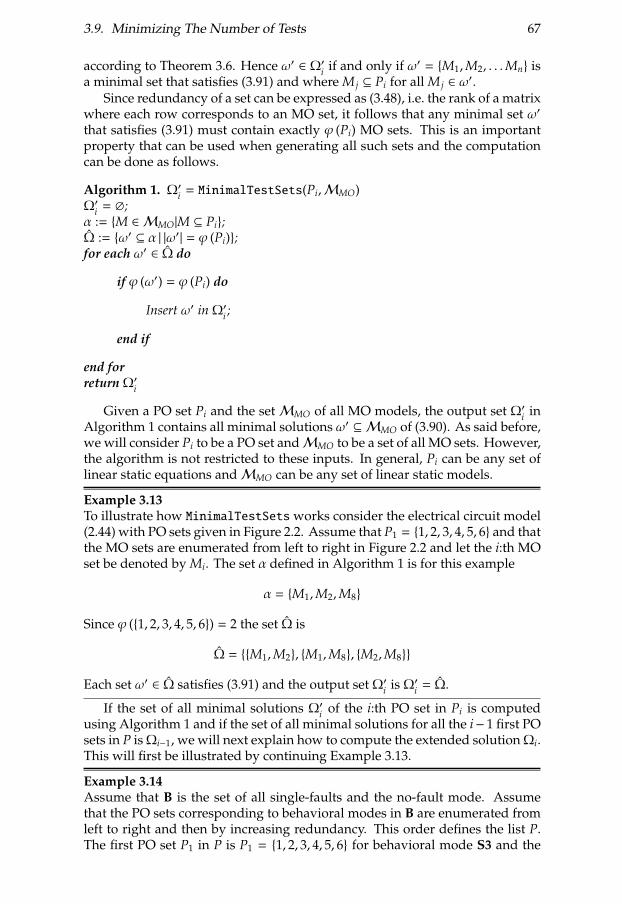
3.9. Minimizing The Number of Tests 67

according to Theorem 3.6. Hence ω′ ∈ Ω′i

if and only if ω′ = M1,M2, . . .Mn isa minimal set that satisfies (3.91) and where M j ⊆ Pi for all M j ∈ ω′.

Since redundancy of a set can be expressed as (3.48), i.e. the rank of a matrixwhere each row corresponds to an MO set, it follows that any minimal set ω′

that satisfies (3.91) must contain exactly ϕ (Pi) MO sets. This is an importantproperty that can be used when generating all such sets and the computationcan be done as follows.

Algorithm 1. Ω′i= MinimalTestSets(Pi,MMO)

Ω′i= ∅;

α := M ∈ MMO|M ⊆ Pi;Ω := ω′ ⊆ α | |ω′| = ϕ (Pi);for each ω′ ∈ Ω do

if ϕ (ω′) = ϕ (Pi) do

Insert ω′ in Ω′i;

end if

end forreturn Ω′

i

Given a PO set Pi and the setMMO of all MO models, the output set Ω′i

inAlgorithm 1 contains all minimal solutions ω′ ⊆ MMO of (3.90). As said before,we will consider Pi to be a PO set andMMO to be a set of all MO sets. However,the algorithm is not restricted to these inputs. In general, Pi can be any set oflinear static equations andMMO can be any set of linear static models.

Example 3.13To illustrate how MinimalTestSetsworks consider the electrical circuit model(2.44) with PO sets given in Figure 2.2. Assume that P1 = 1, 2, 3, 4, 5, 6 and thatthe MO sets are enumerated from left to right in Figure 2.2 and let the i:th MOset be denoted by Mi. The set α defined in Algorithm 1 is for this example

α = M1,M2,M8

Since ϕ (1, 2, 3, 4, 5, 6) = 2 the set Ω is

Ω = M1,M2, M1,M8, M2,M8

Each set ω′ ∈ Ω satisfies (3.91) and the output set Ω′i

is Ω′i= Ω.

If the set of all minimal solutions Ω′i

of the i:th PO set in Pi is computedusing Algorithm 1 and if the set of all minimal solutions for all the i− 1 first POsets in P isΩi−1, we will next explain how to compute the extended solutionΩi.This will first be illustrated by continuing Example 3.13.

Example 3.14Assume that B is the set of all single-faults and the no-fault mode. Assumethat the PO sets corresponding to behavioral modes in B are enumerated fromleft to right and then by increasing redundancy. This order defines the list P.The first PO set P1 in P is P1 = 1, 2, 3, 4, 5, 6 for behavioral mode S3 and the


set of all minimal families ω of MO sets that satisfy (2.34) for S3 is according toExample 3.13 equal to

Ω1 = M1,M2, M1,M8, M2,M8

The next PO set in P is P2 = 1, 2, 3, 4, 6, 7, and the set Ω′2 obtained usingAlgorithm 1 of all minimal families of MO sets that satisfy (2.34) for S1 is

Ω′2 = M1,M2, M1,M3, M1,M6, M2,M3, M2,M6, M3,M6

Next, the solutions in Ω1 and in Ω′2 are combined to form a solution whenconsidering both PO set P1 and P2. Sinceω ∈ Ω1 is a solution for P1 andω′ ∈ Ω′2is a solution for P2, it follows that ω ∪ ω′ will be a solution, not necessarilyminimal, to the problem of testing both P1 and P2. By taking the union of allpairs in the setsΩ1 andΩ2 and then remove non-minimal solutions, we obtain

Ω2 = M1,M2,M3, M1,M2,M4, M1,M2,M6, M1,M3,M8, M1,M4,M8,M1,M6,M8, M2,M3,M4,M8, M2,M3,M6,M8, M2,M4,M6,M8

An example of a non-minimal solution that has been removed to obtain this setis M1,M2,M3,M6which is produced by taking the union of M1,M2 ∈ Ω1 andM3,M6 ∈ Ω2. By construction,Ω2 contains all minimal setsω that satisfy (3.49)for both P1 and P2.

In the example we saw that Ωi can be obtained from Ωi−1 and Ω′i

by firstcomputing

Ωi = ω′ ∪ ω|ω ∈ Ωi−1, ω′ ∈ Ω′i (3.92)

and then pruning all non-minimal sets in Ωi. Let these operations be denotedby Extend such that Ωi can be expressed as

Ωi = Extend(Ωi−1,Ω′i ) (3.93)

Remember that P = (P1, . . .Pn) is an ordered set of all PO sets with a be-havioral mode in B. The output is invariant under permutations, but thecomputational complexity is not. The computational complexity is closely re-lated to the size of Ωi in all steps. A large redundancy of a PO set Pi leads ingeneral to a large set Ω′

i. To reduce the size of the initial sets Ωi a heuristic is

then to order the PO sets in increasing redundancy.Now, the main algorithm can now be summarized as follows.

Algorithm 2. Ω = AllMinimalTestSets(P,MMO)Ω = ∅;for i = 1 to n do

Ω′ := MinimalTestSets(Pi,MMO);

Ω := Extend(Ω,Ω′);

end forreturn Ω


Given a list P of PO sets and the setMMO of all MO models, the output setΩ of Algorithm 2 contains all minimal solutions ω ⊆ MMO of (3.89).

The minimum number of tests can now be obtained by testing the MO setsin any minimum cardinality set ω ∈ Ω. Sometimes the set Ω is large andtherefore computationally expensive to compute. Since the objective is to com-pute only one minimum cardinality solution it is not necessary to compute allminimal solutions. By the following small modification of the above describedalgorithm, it is possible to define an algorithm where the output set Ω will bethe set of all minimum cardinality sets ω. If the minimum cardinality sets ωhave cardinality m, then only the minimum cardinality sets ω is obtained in theoutput of Algorithm 2 if (3.92) is replaced by

Ωi = ω′ ∪ ω|ω ∈ Ωi−1, ω′ ∈ Ω′i , |ω′ ∪ ω| ≤ m (3.94)

The number m can be found as the minimum number that gives a non-emptyoutput set Ω of the modified Algorithm 2 and this set is then the desired set.

Since all minimum cardinality sets can be computed additional objectives,such as computational aspects of the residuals, can be added to chose the bestminimum cardinality set.

3.9.2 Examples

Now, both Theorem 3.10 and Algorithm 2 will be used to obtain MO sets ω forsome variants of the electrical circuit example.

Example 3.15First, consider again the electrical circuit when the set B contains all multi-ple fault behavioral modes and the no-fault mode. This means according toFigure 2.2 that the input list P in Algorithm 2 contains all PO sets andMMO con-tains all MO sets in Figure 2.2. The output set Ω contains in this case only oneminimal set ω =MMO including all MO sets in Figure 2. ThereforeMMO is theunique minimum cardinality solution. This means that the minimal number oftests required to obtain soundness is 8.

To explain the result, take for instance behavioral mode R1&R2 with itscorresponding behavioral model 1, 4, 5, 6, 7. The MO set 4, 5 is the only POset with the same observation set as 1, 4, 5, 6, 7. Hence to fulfill (2.34) forbehavioral mode R1&R2, the MO set 4, 5 has to be included in ω. This can beseen in Figure 2.2 where R1&R2 is among the behavioral models listed below4, 5. In the figure, it can be seen that each MO set has an observation set equalto an observation set to some behavioral model. Therefore, all MO sets must inthis case be included in ω.

Example 3.16Assume this time that only single faults are to be considered, i.e. B = NF,R1, R2, B, S1, S2, S3. For soundness, it is required that the consistency of allbehavioral models Mb such that b ∈ B can be determined. By looking at theHasse diagram in Figure 2.2, it can be seen that this is equivalent to determinethat consistency of all PO sets with redundancy 2 and 3.

Since the model equations are the same as when considering all multiplefaults, Theorem 3.10 again implies that all 8 MO sets are sufficient. Another


possibility to satisfy (2.34) for all b ∈ B is to include the 5 PO sets with redun-dancy 2 in ω. However the redundancy is 2 for each PO set and this choice cantherefore be seen as testing the consistency of 5 × 2 = 10 consistency relationscompared to test the 8 MO sets.

Not all MO sets need to be tested in order to fulfill (2.34) for all behavioralmodes in B = NF, R1, R2, B, S1, S2, S3. To compute the minimum numberof MO sets needed Algorithm 2 is applied to the inputs P equal to the set ofall PO sets with redundancy 2 and 3 andMMO equal to the set of all MO setsin Figure 2.2. The output set Ω contains 13 minimal sets of which 12 are ofminimum cardinality 5. One of these minimum cardinality sets is

ω = 1, 2, 3, 4, 6, 1, 2, 3, 6, 7, 1, 2, 5, 6, 7, 3, 4, 7, 4, 5

Hence the minimum number of tests is 5.

In the following two examples, an extension to the electrical circuit modelis considered.

Example 3.17Next all multiple faults are again considered. In addition to the model givenin (2.44), the battery is modeled to two behavioral modes B ∈ NF,F where Fstands for ”faulty”. A faulty battery is assumed to have no voltage across thebattery, i.e. V = 0 if B = F. The extended model becomes

Assumption Equation Expression(1) I − I1 − I2 = 0

R1 = NF (2) V − I1 R1 = 0R2 = NF (3) V − I2 R2 = 0B = NF (4) V −U = 0S1 = NF (5) V − yV = 0S2 = NF (6) I − yI = 0S3 = NF (7) I2 − yI2 = 0B = F (8) V = 0

(3.95)

The equations 4 and 8 are mutually exclusive. The set 4, 8 is therefore anexample of an MO set that is not a feasible model. This MO set need not beconsidered according to Theorem 3.10. Since a subset of a feasible model isfeasible, the set of all feasible models can be represented as all subsets of themaximal feasible models. The maximal feasible models in the example areM\8 = MNF and M\4 = MB. The Hasse diagram for (3.95) is shown inFigure 3.1. This shows the subset relation of all feasible PO sets for the model.The two maximal feasible models are the ones on redundancy level 3.

The additional feasible MO sets found in the extended model (3.95) are1, 2, 3, 6, 8, 1, 2, 6, 7, 8, 3, 7, 8, 5, 8. If the input list P in Algorithm 2 containsall PO sets with behavioral modes in Figure 3.1 andMMO contains all MO setsin Figure 3.1, then the output set Ω consists of one minimal set ω includingthe 8 MO sets in Figure 3.1 with behavioral modes. Hence it is necessaryand sufficient to check the consistency of all 8 MO sets which includes eitherequation 4 or 8. The matrices NH[Mi] L for the MO sets Mi ∈ M are the ones


1,2,3,4,5,6,7

NF

1,2,3,5,6,7,8

B

1,2,3,4,5,6

S3

1,2,3,4,6,7

S1

1,2,4,5,6,7

R2

3,4,5,7

R1,S

2,R

1&

S2

1,2,3,5,6,7

1,2,

3,5,

6,8

B&

S3

1,2,3,6,7,8

B&

S1

1,2,5,6,7,8

R2&

B

3,5,7,8

R1&

B,B

&S

2,R

1&

B&

S2

1,2,3,4,6

S1&

S31,2,4,6,7

R2&

S1

3,4,7

R1&

S1

S1&

S2

R1&

S1&

S2

4,5

R1&

R2

R1&

S3

R2&

S2

R2&

S3

S2&

S3

R1&

R2&

S2

R1&

R2&

S3

R1&

S2&

S3

R2&

S2&

S3

R1&

R2&

S2&

S31,2,3,5,61,2,3,6,71,2,5,6,73,5,71,2,3,6,8

B&

S1&

S3

1,2,

6,7,

8R

2&

B&

S13,7,8

R1&

B&

S1

B&

S1&

S2

R1&

B&

S1&

S2

5,8

R1&

R2&

BR

1&

B&

S3

R2&

B&

S2

R2&

B&

S3

B&

S2&

S3

R1&

R2&

B&

S2

R1&

R2&

B&

S3

R1&

B&

S2&

S3

R2&

B&

S2&

S3

R1&

R2&

B&

S2&

S3

Figu

re3.

1:A

llfe

asib

lePO

subs

ets

of(3

.95)

.


shown in (3.88) and

MO U yV yI yI2

1, 2, 3, 6, 8 [ 0 0 1 0 ]1, 2, 6, 7, 8 [ 0 0 1 −1 ]3, 7, 8 [ 0 0 0 1 ]5, 8 [ 0 1 0 0 ]

(3.96)

Example 3.18The last example is to consider the model in (3.95) but now with B = NF,R1,R2, B, S1, S2, S3. Let the input list P in Algorithm 2 contain all PO sets inFigure 3.1 with behavioral modes in B = NF,R1, R2, B, S1, S2, S3 and letMMO contain all MO sets in Figure 3.1. The output set Ω contains 73 minimalsets of which 63 are of minimum cardinality 6. If the MO sets Mi are enumeratedfrom left to right in Figure 3.1 one such set is

ω = M1,M2,M4,M5,M8,M9

The number of minimal solutions ω is large if P includes few PO sets withlow redundancy, as in the single fault examples, compared to the case whenmany MO sets are included in P, as in the multiple fault examples. Since thecomputational complexity of finding all minimum cardinality sets ω dependson the number of solutions ω, the same can be said about the computationalcomplexity of computing Ω.

3.10 Fault Influence on Residuals

In the diagnosis system design approach used here, i.e. starting from the modelas described in Section 2.3.3, the idea is to construct residuals for MO sets. Anytest quantity based on the MO set M of equations Hx+Lz+ c = 0 can be writtenwith some basis NH of the left null space of H as

r = NH(Lz + c) (3.97)

A scaling factor is the only design freedom for a residual based on the MO setM. Since scaling does not affect which faults that the residual r is influenced by,any residual based on the same MO set will be influenced by the same faults.

Fault influence on residuals is typically analyzed when faults are modeledwith fault variables. In this case a residual r is said to be influenced by a faultF, if the residual r is sensitive to a change in the corresponding fault variablef , i.e. if f , 0 implies that r , 0 in the linear case. In the framework used here,faults need not be explicitly modeled with fault variables and the meaning offault influence on a residual can not be defined in this way. A formulation offault influence that generalizes to the situation without fault variables is thefollowing. In the linear case, it is equivalent that a residual r is sensitive to afault variable f corresponding to fault F and that r , 0 is consistent with theassumption that the system to be diagnosed is in fault mode sys = F. To makethe next definition generally valid, we will use behavioral mode instead of faultmode.

3.10. Fault Influence on Residuals 73

Definition 3.6 (Influenced by a Behavioral Mode). A residual r is influenced bya behavioral mode b if

∃z ∈ O(Mb) : r(z) , 0 (3.98)

This means that a residual r is influenced by a fault mode F if r , 0 isconsistent with the behavioral model MF. This formulation of fault influencedoes not require that the fault F is explicitly modeled with a fault variable f .Hence this is what we mean with fault influence on a residual r in the generalcase.

In this section the fault influence on a residual r based on an MO set Mis investigated and the main result is, under some general assumptions givenlater, that the r is influenced by the faults, or more general the behavioralmodes, b ∈ (assump(M))C. Before a general linear static model is discussed, wewill consider a special case where all faults are explicitly modeled with faultvariables.

3.10.1 Fault Influence in Models with Fault Variables

Assume that the no-fault behavior of a process can be described by the linearstatic model

H′ x + L′ z = 0 (3.99)

Furthermore, assume that there are m single faults modeled by a vector f . Forthe variable fi it holds that fi = 0 if fault i is not present. The static linearmodel (2.26) would then be

H′x + L′z + F′ f = 0 (3.100)

This model can be written in the framework used here as follows. Each fault ican be related to a component ci which can either be in the no-fault mode NFor the faulty mode F. The model then becomes

c1 =NF f1 = 0...

...cm =NF fm = 0

H′x + L′z + F′ f = 0

(3.101)

The variables in f are considered to be unknown variables. Assume that we pickout an MO set of equations in (3.101). These equations can, after a renumerationof the faults, be written as

c1 =NF f1 = 0...

...cn =NF fn = 0

Hx + Lz + F f = 0

(3.102)

where n ≤ m. Let the fault vector f be partitioned such that the n first faultvariables f1, . . . , fn form a vector f a and the rest of the faults are included in f b,i.e.

f =

[

f a

f b

]

(3.103)


Furthermore, let Fa = F[:, 1, . . . ,n] and Fb = F[:, n + 1, . . . ,m]. The modelequations (3.102) can now be written in the form (3.5) as

H︷︸︸︷[

I 0 0Fa Fb H

]

x︷︸︸︷

f a

f b

x

+

L︷︸︸︷[

0L

]

z = 0 (3.104)

Any residual for this MO set can be written as

r = NHLz (3.105)

where the scaling α in (3.97) can be included in NH. To find out the faultinfluence on the residual r, we want to express r only in the fault vector f .

To do this, we will first express the residual with the sub-matrices givenin (3.104). Let the row-vector NH be partitioned into [N1 N2]. Since NHH = 0we get that

[

N1 N2

][

I 0 0Fa Fb H

]

=[

N1 +N2Fa N2Fb N2H]

= 0 (3.106)

This implies thatN2 = N[Fb H] (3.107)

and then also thatN1 +N[Fb H]Fa = 0 (3.108)

From that NH = [N1 N[Fb H]] and the definition of L in (3.104), it follows that theresidual in (3.105) can be expressed as

r = NHLz =[

N1 N[Fb H]

][

0L

]

z = N[Fb H]Lz (3.109)

Now, by multiplying the lower part of (3.104) with N[Fb H], we get

N[Fb H]Fa f a +N[Fb H]Fb f b +N[Fb H]Hx +N[Fb H]Lz = 0 (3.110)

On the left-hand side the second and third term is zero and the last term isaccording to (3.109) equal to r. This means that the residual is equal to

r = −N[Fb H]Fa f a (3.111)

Finally, by using (3.108) and that N1 = NH[:, 1, . . . ,n], the fault influence onthe residual r is given by

r = NH[:, 1, . . . ,n] f a (3.112)

The residual is influenced by all faults in f a where the corresponding columnin the row-vector NH[:, 1, . . . ,n] is non-zero. Since (3.102) is an MO set ofequations, it follows from Corollary 3.1 that all columns in NH are non-zero anda consequence of this is that all columns in NH[:, 1, . . . ,n] are non-zero. Hencethe residual r in (3.105) is influenced by all faults in f a and not influenced byany faults in f b. An interpretation of (3.107) is that the faults f b are decoupledand it will be shown that the resulting residual will not be influenced by anyfault in f b. Hence the partition of the faults in (3.103) can be interpreted as notdecoupled faults f a and decoupled faults f b. The result of this discussion issummarized in the following theorem.


Theorem 3.11. Given a linear static model where all faults are modeled explicitly asin (3.101) and an MO subset of equations (3.102), any residual r = NHLz using thenotation in (3.104) will have the fault influence

r =[

NH[:, 1, . . . ,n] 0][

f a

f b

]

(3.113)

where NH[:, i] , 0 for all i ∈ 1, . . . ,n.

Proof. The theorem follows directly from the formal discussion starting with (3.101)and ending with Theorem 3.11.

Usually, we will start with a diagnosis model with the set M of equa-tions (3.101) and form a residual based on an MO set M ⊆ M. If the set M ofequations (3.101) is written on matrix form with matrices H′ and L′, then theresult of Theorem 3.11 can then be reformulated in terms of matrices H′ andL′ as follows. Given any MO set M ⊆ M, any residual based on M can the bewritten

r = NH′[M]L′z (3.114)

and its fault influence is given by

r = NH′[M][:, 1, . . . ,m] f (3.115)

according to Theorem 3.11.

Example 3.19To exemplify the result of Theorem 3.11 consider the model

[

11

]

x +

[

1 00 1

]

z +

[

1 0 10 1 1

]

f = 0 (3.116)

which written in the form (3.101) is

c1 = NFc2 = NFc3 = NF

1 0 0 00 1 0 00 0 1 01 0 1 10 1 1 1

f1f2f3x

+

0 00 00 01 00 1

z = 0 (3.117)

where the matrices are called H′ and L′ respectively. This model includes oneMO set, i.e. the set 1, 2, 4, 5. By computing the vector

NH[1,2,4,5] =[

−1 1 0 1 −1]

a residual and its fault influence is then given by

r =[

1 −1]

z =[

−1 1 0]

f (3.118)

according to (3.114) and (3.115) respectively.


3.10.2 Fault Influence in General Linear Static Models

In the previous discussion all faults were explicitly included in the model asfault variables and then it was possible to quantify the influence of a fault ona residual. The next theorem generalizes the result in Theorem 3.11 to generallinear static models described in Section 3.6.

Theorem 3.12. Let M be an MO set of linear equations

H x + L z + c = 0 (3.119)

where rank ([H L c]) = rank ([H L]) and let model deviation be described by a vector ǫsuch that

H x + L z + c = ǫ (3.120)

Any residual derived from M can be written

r = NH(Lz + c) (3.121)

and the residual response of the model deviation is given by

r = NHǫ (3.122)

where NH[:, i] , 0 for all i ∈M.

Proof. Since (3.119) is an MO sets, it has redundancy one. This means that NH isa vector determined up to a non-zero constant. By multiplying (3.120) with NH

from the left, we get both the residual computational form (3.121) and the faultresponse (3.122). Since M is an MO set Corollary 3.1 states that all columns inNH are non-zero, i.e. NH[:, i] , 0 for all i ∈M.

According to (3.122) almost any model deviation ǫ , 0, i.e. for all ǫ ∈ R|M|except for a line, will be detected with the residual r. To see how Theorem 3.12is a generalization of Theorem 3.11 apply the result of Theorem 3.12 to themodel (3.102) which expressed on matrix form is given in (3.104). By addingthe model deviation ǫ, we get

Hx + Lz = ǫ (3.123)

From the n first equations, it follows that fi = ǫi for 1 ≤ i ≤ n. The remainingequations are true in any behavioral mode, i.e. ǫi = 0 for all i ≥ n + 1. Byelimination of ǫ in (3.122) we get an expression equivalent to (3.113).

Example 3.20To give an example of the result of Theorem 3.12 consider the electrical circuitmodel in (3.3). The faults in this model are not described with fault variablesf and it is therefore not possible to use Theorem 3.11. As suggested in The-orem 3.12 a model deviation vector ǫ is added to the model. Since the firstequation in (2.44) is true for all behavioral modes, it follows that ǫ1 = 0. Withthe matrices H and L defined as in (3.3) the fault influence for the MO sets Mi

in (3.88) are given byri = NH[Mi]Lz = NH[Mi]ǫ (3.124)


The fault sensitivity is directly given by the coefficients in the matrix NH[Mi]. Togive an example assume that the resistor 1 is broken and the fault appears suchthat V1 − I1R1 = ǫ2 where ǫ2 , 0. Then the residuals ri will be equal to

ri = NH[Mi][:, 2]ǫ2 (3.125)

according to (3.124). This means that the residuals that are based on an MOsets that include equation 2 are the residuals that will be non-zero.

3.10.3 Fault Influence and Null Hypothesis

In the framework used in this thesis, conclusions are drawn only when r ∈ Raccording to (2.7), i.e. if r ∈ R then the null hypothesis sys ∈ Φ of the test isrejected. To draw the strongest conclusion when r ∈ R, the set ΦC should bechosen to be exactly the set of behavioral modes that influence the residual r.

By using the fault influence given in Theorem 3.12 the next theorem showsthat the fault influence is given by the model assumptions, i.e. the fault influenceis assump(M)C. In the theorem, we will denote the column-span of a matrix Aby Im(A).

Theorem 3.13. LetM be a diagnosis model with the set M of equations

Hx + Lz + c = 0 (3.126)

where

rank ([H[M] L[M] c[M]]) = rank ([H[M] L[M]) (3.127)

for all maximal feasible models M ⊆M. Let the model deviation be modeled as

Hx + Lz + c = Fǫ (3.128)

where F is a |M| × |M| matrix defined by

Fi j =

1 if i = j and assump(ei) , B

0 otherwise(3.129)

If

Im(F) ⊆ Im([H L]) (3.130)

then for any MO set M ⊆M of equations and for any residual

r = NH[M]Lz (3.131)

not identically zero and based on M, r is influenced by all behavioral modes in(assump(M))C and no others.

From Theorem 3.12 we do know that a residual r based an MO set M willbe sensitive to all model deviation variables ǫi included in the equations M.Condition (3.130) guarantees that there exists a non-zero ǫ such that r , 0, i.e.the model deviation variables ǫi can be seen as independent input signals.


Proof. An MO set M and a residual r are given. We start to prove that r is notinfluenced by any behavioral mode b ∈ assump(M). By the definition of theoperator assump, it follows that

sys ∈ assump(M)→ z ∈ O(M) (3.132)

The observation set O(M) can according to (3.10) and (3.131) be expressed as

O(M) = z|NH[M]Lz = 0 = z|r(z) = 0 (3.133)

The formulas (3.132) and (3.133) imply that

sys ∈ assump(M)→ r = 0 (3.134)

i.e. r is not influenced by any behavioral mode b ∈ assump(M).Now, we continue to prove that r is influenced by all behavioral modes b <

assump(M). The idea is to take an arbitrary behavioral mode b ∈ (assump(M))C

and show that the equations Mb and r , 0 are consistent. From the definitionof the operator assump, it follows for any set M that

M ⊆Mb → b ∈ assump(M)

Then, since b < assump(M), it follows that M *Mb or equivalently that M\Mb ,

∅. Let M \ Mb be denoted by M′. By construction of M′, it follows thatb < assump(e) for any e ∈ M′. This implies that assump(e) , B for all e ∈ M′,i.e., F[M′,M′] is the identity matrix. From (3.128), (3.131), and (3.122), we getthe fault influence

r = NH[M]Fǫ (3.135)

The only equations e ∈ M that might be inconsistent, i.e. ǫ[e] , 0, are theequations e ∈M′. Hence (3.135) can be rewritten as

r = NH[M][:,M′]F[M′,M′]ǫ[M′] = NH[M][:,M′]ǫ[M′] (3.136)

From (3.130) it follows that

Im(F[M ∪Mb]) ⊆ Im([H[M ∪Mb] L[M ∪Mb]]) (3.137)

i.e. for any ǫ[M ∪Mb] there exist some x and z such that the subset M ∪Mb ofthe equations in (3.128) is satisfied. Since M′ ∩Mb = ∅, we can choose ǫ[M′]such that r , 0 in (3.136) and ǫ[Mb] = 0. This implies that we have found an ǫsuch that Mb is consistent in (3.128) according to (3.126), and r , 0. Since b wasan arbitrarily chosen behavioral modes such that b < assump(M), it followsthat r is influenced by all behavioral modes in (assump(M))C and the theoremfollows.

Next two remarks of this theorem will be discussed. First, note that asufficient condition for (3.130) is that [H L] has full row-rank. This means thatTheorem 3.13 is not restrictive for diagnosis models where all equations arevalid in the no-fault mode. However Theorem 3.13 becomes restrictive in thecase with several maximal feasible models.

Second, the fault influence on a residual derived from an MO set M is(assump(M))C for the class of models consider in Theorem 3.13. This means


that the set Φ in (2.7) should according to the fault influence be chosen asΦ = assump(M). This is in agreement with the guideline (2.15) presented inSection 2.2.1.

The next corollary restates Theorem 3.13 for an important special case of theclass of models handled in Theorem 3.13, i.e. the type (3.101).

Corollary 3.4. LetM be a diagnosis model with the set M of equations

c1 =NF f1 = 0...

...cn =NF fn = 0

Hx + Lz + F f = 0

(3.138)

IfF ⊆ Im([H L]) (3.139)

then for any MO set M ⊆ M of equations and for any residual r not identically zeroand based on M, r is influenced by all faults in (assump(M))C and no others.

Proof. The proof is immediate from Theorem 3.13.

Now, we will illustrate the result of Theorem 3.13 by three examples. Thefirst and second example show when the condition (3.130) is met and the conclu-sion of theorem follows. The third example illustrates the case when (3.130) isnot fulfilled and it shows why the fault influence (assump(M))C is not obtainedin this case.

Example 3.21The continuation of Example 3.19. It can be verified that (3.130) is true eitherby using the matrices H′ and L′ in (3.117) and

F′ =

[

I3×3 03×202×3 02×2

]

or with the matrices H, L, and F in (3.116), i.e.

F =

[

1 0 10 1 1

]

H =

[

11

]

L =

[

1 00 1

]

The assumption of the MO set 1, 2, 4, 5 is assump(1, 2, 4, 5) = φ(c1 = NF∧c2 =

NF), i.e. the residual (3.118) is according to Theorem 3.13 or Corollary 3.4influenced by all faults in

(assump(1, 2, 4, 5))C = (φ(c1 = NF ∧ c2 = NF))C = φ(c1 = F ∨ c2 = F)

This can also be directly seen in (3.118) and it means that it is possible to detectall faults modes in the complement set of assump(1, 2, 4, 5).

Example 3.22For the electrical circuit example with the model (3.95) it holds that [H L] hasfull row rank. This is a sufficient condition for (3.130) and it follows that forany residual r based on an MO set M, (assump(M))C are the behavioral modesthat r is influenced by.


Next an example shows what can happen when (3.139) is not fulfilled.

Example 3.23Consider the model

c1 =NF f1 = 0c2 =NF f2 = 0

H︷︸︸︷

111

x +

L︷︸︸︷

−1 0−1 00 −1

z +

F︷︸︸︷

1 01 10 1

f = 0

(3.140)

The set 1, 2, 3, 5 is an MO set and a residual is

r = y1 − y2 = f1 − f2 (3.141)

From this expression we would expect that r is influenced by c1 = NF ∧ c2 =

F which is contained in (assump(M))C. We will show that this is not trueand (3.139) is not fulfilled for this example.

It can be verified that F * Im([H L]). It is the column corresponding to f2that does not satisfy (3.139) and f2 cannot be chosen arbitrarily. In fact, thelast three equations in (3.140) implies that f2 = 0 in any behavioral mode. Bysubstitution of f2 in (3.141) the fault influence is given by

r = y1 − y2 = f1

Hence behavioral modes that influences r are φ(c1 = F) ⊂ (assump(M))C.

Note that even if the fault influence on a residual based on M is equal toB ⊂ (assump(M))C, it is possible to use Φ = assump(M) as null hypotheses.The effect is that when the r , 0 then it is concluded that sys ∈ (assump(M))C

but according to the model r , 0 means that sys ∈ B. However if there is oneresidual ri for each model Mi in a setω that satisfies (2.34) then exactly the samecandidates will be obtained if Φi = assump(Mi) or if Φi is equal to the true faultinfluence of ri. Hence when designing a sound diagnosis system the exact faultinfluences on each residual ri is not important.

3.11 Conclusions

In Chapter 2 we showed that one strategy to construct a diagnosis system was tostart with a diagnosis modelM and choose a set ω = M1, . . . ,Mn of rejectablemodels to test. There, it was also shown that a diagnosis system based on ωcan be sound and complete if and only if the setω fulfills (3.1) for all behavioralmodes b ∈ B.

This chapter has presented theory and algorithms for finding a minimumcardinality solution ω of (3.1) given a diagnosis model M with linear staticequations. A key result is that if ω is chosen to be the set of all feasible MOsets in the diagnosis model M, then ω fulfills (3.1) for all behavioral modesb ∈ B according to Theorem 3.10. It has also been shown that it is not ingeneral necessary to include all MO sets in ω to satisfy (3.1) for all behavioralmodes b ∈ B. Theory for selecting MO sets has been developed and a key

3.11. Conclusions 81

result for this is the rank condition given in Theorem 3.6. The rank conditionis then used in Algorithm 2 for selecting MO sets. The output of the algorithmcontains all minimal subsets ω that fulfill (3.1) for all behavioral modes b ∈ B.A minimal cardinality set of MO sets is then picked out from the set of allminimal sets. Note that this is important because, a minimum cardinality set ωthat satisfies (3.1) for all behavioral modes b ∈ B, corresponds to a sound andcomplete diagnosis system with the minimum number tests. Several examplesof the minimization of the number of tests in the design of a sound and completediagnosis systems have been given in Section 3.9.

Finally, Theorem 3.13 showed that under a mild rank condition on thediagnosis model and given an MO set M, the behavioral modes that influenceany residual derived from M are given by the equation assumptions accordingto (assump(M))C. Hence if the rank condition of the model can be verified, thenany further fault influence analysis of each residual is not needed.

4

A E A FMO S

In the previous chapter we have shown in Theorem 3.10 that a sound diagnosissystem can be based on all feasible MO sets in a diagnosis model M, i.e., allMO sets M in M such that assump(M) , ∅. In this chapter an algorithmfor computing all MO sets in a linear static or dynamic model is proposed.How to apply the algorithm to dynamic models will be discussed later inChapter 6. The algorithm developed here will also be the basis for constructinga structural algorithm that can be applied to models containing non-lineardifferential equations in Chapter 9.

All MO sets in a diagnosis model are in general not feasible MO sets. Thealgorithm presented in this chapter finds all MO sets in a model, both feasibleand non-feasible ones. It is not computationally efficient to find all MO setsand then remove the non-feasible ones to get only the feasible MO sets. InChapter 5 an algorithm is constructed for finding only feasible MO sets. Thealgorithm presented here will be the key component in the construction of thealgorithm for finding only feasible MO sets.

Section 4.1 and 4.2 introduce key concepts that will be used in the construc-tion of the algorithm. In Section 4.3 a basic algorithm for finding all MO setswill be presented. This algorithm illustrates the basic ideas and then in Sec-tion 4.4 further improvements are described. The computational complexity ofthe algorithm is discussed in Section 4.5. Section 4.6 describes step by step theprogress of the algorithm when applied to an illustrative example. Finally theconclusions are drawn in Section 4.7.

4.1 Introduction

We will, as said before, present an algorithm for computing all MO sets in alinear model

Hx + Lz = 0 (4.1)

83

84 Chapter 4. An Efficient Algorithm for Finding all MO Sets

The matrices H and L are scalar matrices in the static case and polynomialmatrices in the dynamic case. In the continuation of this chapter the exampleswill be static. Dynamic examples will later be presented in Chapter 6.

The main idea of the algorithm can be explained by looking at the Hassediagram in Figure 2.2. The algorithm is based on a top-down approach inthe sense that we start with the entire model and then reduces the size andthe redundancy of the model step by step until an MO set remains. For theHasse diagram in Figure 2.2 we start with 1, 2, 3, 4, 5, 6, 7 and, by for examplefollowing the rightmost branch in the graph, 3, 4, 5, 7 and then the MO set 4, 5is obtained. How to obtain PO sets with decreasing redundancy is describedin the next section.

4.2 The Proper Overdetermined Part

As said in the introduction, the idea is to find MO sets in a PO set by computinga sequence of PO subsets with decreasing redundancy until an MO set is found.

Example 4.1For the electrical circuit example with PO sets shown in Figure 2.2, the MOset 4, 5 can be obtained by starting with the PO set 1, 2, 3, 4, 5, 6, 7 with re-dundancy 3 and then compute the PO subset 3, 4, 5, 7with redundancy 2 andfinally compute the MO set 4, 5.

This motivates studying how to compute a PO sets E ⊂M′ with redundancyϕ − 1, given a PO set M′ with redundancy ϕ ≥ 2. Such computation can bedivided into the following two steps:

a) Remove an arbitrary equation e ∈M′ from M′ and let M =M′ \ e.

b) Find a PO set E ⊆M ⊂M′ with redundancy ϕ − 1.

The rest of this section is organized as follows. First, the existence and unique-ness of the PO set E, specified in step (b), are shown. Then, a method to computethe PO set E given a model M is proposed.

4.2.1 Existence and Uniqueness

The existence and uniqueness of the PO set E, specified in step (b), are shownin the following theorem.

Theorem 4.1. Given a PO set M′ with redundancy ϕ (M′) ≥ 2 and an arbitraryequation e ∈M′, there exists a unique PO set E ⊆M′\e such thatϕ (E) = ϕ (M′)−1.

The uniqueness part of the proof of this theorem will be based on the twofollowing lemmas. In these lemmas we will use the notation of supermodu-larity, i.e., the redundancy function ϕ is a super-modular function on P(M)if

ϕ (M1 ∪M2) + ϕ (M1 ∩M2) ≥ ϕ (M1) + ϕ (M2) (4.2)

for any sets M1 ⊆M and M2 ⊆M.

Lemma 4.1. If M is a set of equations defined by (3.5) where [H L] has full row-rank,then the redundancy function ϕ is a super-modular function on P(M).

4.2. The Proper Overdetermined Part 85

Proof. A function is super-modular if (4.2) holds for all subsets M1 ⊆ M andM2 ⊆M. Since [H L] has full row-rank, it follows that

ϕ (M′) = |M′| − rank (H[M′]) (4.3)

for all M′ ⊆M. By using this, (4.2) is true if

|M1 ∪M2| − rank (H[M1 ∪M2]) + |M1 ∩M2| − rank (H[M1 ∩M2])≥ |M1| − rank (H[M1]) + |M2| − rank (H[M2])

is true. Simplification of this inequality by using that

|M1 ∪M2| + |M1 ∩M2| = |M1| + |M2|

gives

rank (H[M1 ∪M2]) + rank (H[M1 ∩M2]) ≤ rank (H[M1]) + rank (H[M2])

which is the definition of the rank-function being sub-modular. The sub-modularity of the rank-function follows from Lemma 3.1 and this completesthe proof.

Lemma 4.2. Let M be a set of equation such that ϕ (M) ≥ 1 and such that theredundancy function ϕ is a supermodular function on P(M). Then there existsa unique PO set E ⊆ M with maximal redundancy among all subsets of M, i.e.,ϕ (E) = ϕ (M).

A more general formulation of this lemma is stated and proved in (Ore,1956).

Proof. Theorem 3.3 states that ϕ (E) ≤ ϕ (M) for all subsets E ⊆ M. From thisand that M1 ∪M2 ⊆M and M1 ∩M2 ⊆M, it follows that

ϕ (M1 ∪M2) + ϕ (M1 ∩M2) ≤ 2ϕ (M) (4.4)

Assume that M1 and M2 are two PO sets with redundancy ϕ (M) ≥ 1. Sinceϕ is a supermodular function on P(M), it follows that (4.2) holds for any setsM1 ⊆ M and M2 ⊆ M. This, (4.2), and (4.4) imply equality in (4.2). From thisand the fact that M1 and M2 have maximal redundancy among the subsets ofM, it follows that

ϕ (M1 ∩M2) = ϕ (M1) = ϕ (M2)

From this, M1 ∩M2 ⊆M1, M1 ∩M2 ⊆M2, and M1 and M2 are PO sets, i.e.,

ϕ (E) < ϕ (Mi) (4.5)

for all proper subsets E ⊂Mi, we get

M1 =M1 ∩M2 =M2

i.e., M1 = M2. Since M1 and M2 was chosen to be two arbitrary PO sets in Mwith maximal redundancy, it follows that there exists a unique PO set in M withmaximal redundancy.

Now, we are ready to prove Theorem 4.1.


Proof. We start to prove the existence of a PO set E ⊆M′ \ ewith redundancyϕ (M′) − 1. Since M′ is a PO set with ϕ (M′) ≥ 2, it follows that the resulting setM =M′ \ e has redundancy ϕ (M) = ϕ (M′) − 1 ≥ 1 according to Theorem 3.4.The existence of a minimal set E ⊆ M with redundancy ϕ (M) is trivial. Thensince E is a minimal set with redundancy ϕ (M) ≥ 1, Theorem 3.3 implies thatE is a PO set.

Next the uniqueness is shown. Since M′ is a PO set, it follows that thecorresponding matrix [H L] has full row-rank according to Theorem 3.5. Thisimplies that the matrix [H[M] L[M]] corresponding to the set M also has fullrow rank, i.e., M fulfills the rank condition in Lemma 4.1. This means that theredundancy function ϕ is a supermodular function on P(M). From Lemma 4.2we then get that there exists a unique PO set E ⊆ M with redundancy ϕ (E) =ϕ (M).

The PO set E specified in step (b), is according to Theorem 4.1 the uniquePO set E ⊆ M with maximal redundancy. If we relax the requirement on Msuch that M is any set of equations such that [H L] has full row rank, the super-modularity implies that among the subsets E ⊆ M there exists a unique PO setwith maximal redundancy ϕ (M). This PO set will be denoted by M∗ and willbe called the proper overdetermined (PO) part of M. The set M is in (Ore, 1956)suggested to be partitioned into M∗ ∪ (M \M∗) such that

ϕ (M) = ϕ (M∗) (4.6)

andϕ (M \M∗) = 0 (4.7)

This equations follows from (4.2) when M1 = M \M∗ and M2 = M∗ and theequation (4.6). This means that M∗ contains all redundancy of M and O(M∗) =O(M) according to Theorem 3.6.

Looking back on the two computation steps formulated in the beginning ofthis section, step (b) can be reformulated using the PO part as follows:

b) Find the PO part M∗ of M.

Next a method to compute the PO part M∗ of M will be developed.

4.2.2 Computing the PO Part

The PO part M∗ of M can for example be computed as the set of non-zerocolumns in an arbitrary basis for the left null-space of H as the next theoremshows.

Theorem 4.2. If M is a set of equations in the form (3.5) where [H L] has full row-rank,then

M∗ = e ∈M|NH[:, e] , 0 (4.8)

Before we prove the theorem, let us again consider Example 4.1.

Example 4.2The PO set 3, 4, 5, 7 can be computed from 1, 2, 3, 4, 5, 6, 7 as follows. Since

4.2. The Proper Overdetermined Part 87

1, 2, 3, 4, 5, 6, 7 is a PO set, it follows from Theorem 3.5 that the correspond-ing matrix [H L] has full row-rank. Hence the redundancy function is super-modular on the family of subsets of 1, 2, 3, 4, 5, 6, 7. By removing an equation,lets say the first one, we obtain

ϕ (2, 3, 4, 5, 6, 7) = 2 (4.9)

From the uniqueness of a PO set with redundancy 2 and that ϕ (3, 4, 5, 7) = 2,it follows that

2, 3, 4, 5, 6, 7∗ = 3, 4, 5, 7 (4.10)

From Theorem 4.2 the computation of 2, 3, 4, 5, 6, 7∗ can be done by finding thenon-zero columns of

NH[2,3,4,5,6,7] =

[

0 0 1 0 −1 0 R20 0 0 1 −1 0 0

]

(4.11)

Note that the matrix is zero-padded in accordance with the notation NH[2,3,4,5,6,7].In this way, it is possible to compute PO sets with decreasing redundancy.

Next, we prove Theorem 4.2.

Proof. Let M′ be the set defined by the right-hand side of (4.8). First, we showthat ϕ (M′) = ϕ (M). From the definition of null-space, it follows that the rowsM\M′ in H corresponding to zero columns in NH are linearly independent, i.e.,

rank (H) = rank (H[M′]) + |M \M′| (4.12)

This and that [H L] has full row-rank give

ϕ (M′) = (rank ([H[M′] L[M′]]) + |M \M′|)−(rank (H[M′]) + |M \M′|)

= rank ([H L]) − rank (H) = ϕ (M)

Next, we prove that ϕ (E) < ϕ (M′) for all E ⊂ M′. Since all columns in NH

corresponding to rows in M′ are non-zero, it means that any row in H[M′] islinearly dependent with the other rows, i.e.,

rank (H[M′]) < rank (H[E]) + |M′ \ E| (4.13)

From this and the fact that [H L] has full row-rank, it follows that

ϕ (E) = (rank ([H[E] L[E]]) + |M′ \ E|)−(rank (H[E]) + |M′ \ E|)

< rank ([H[M′] L[M′]]) − rank (H[M′]) = ϕ (M′)

This implies that M′ is a PO set and since ϕ (M′) = ϕ (M) it also follows that M′

has maximum redundancy. Since [H L] has full row-rank, there exist a uniquePO set with maximum redundancy and this is defined to be the PO part M∗ ofM. Hence, it follows that M′ =M∗, i.e., (4.8) is true.


4.3 Algorithm

In this section we will present an algorithm for finding all MO sets. To illus-trate the ideas, a basic version is presented here and then in the next section,improvements are discussed.

4.3.1 Input to the Algorithm

In the algorithm that will be presented next, we start with a set M that willbe assume to be a PO set. A typical input is a behavioral model Mb and anexample of a behavioral model that is a PO set is the no-fault behavioral modelin (3.3) for electrical circuit.

Next we discuss how to obtain a legal input, that is a PO set M, if Mb is nota PO set. If Mb is not a PO set but the corresponding matrix [Hb Lb] has fullrow-rank, then it is easy to obtain M∗

band use this as input.

In the case when [Hb Lb] has not full row-rank, the situation gets morecomplicated. First, check that the rank deficiency is not caused by a modelingerror. If not, there exist two options.

The first option is to compute one PO set M′ ⊂ Mb as follows. A set oflinearly independent rows M ⊂ Mb in [Hb Lb] are identified and then the POpart is computed as M′ = M∗. This set contains all redundancy of Mb and cantherefore be used to check the consistency of Mb.

The second option is to compute all PO sets M ⊆ Mb with maximal redun-dancy and then apply the following algorithm to each of these PO sets. Adisadvantage with this is that the number of MO sets will be greater comparedto the number of MO sets obtained in the first way.

4.3.2 Basic Algorithm

The algorithm will be based on Lemma 3.2, Theorem 3.4, and the followinglemma.

Lemma 4.3. If M is a set of equations in the form (3.5) where [H L] has full row-rank,E ⊆M is a PO set, and e ∈M \ E, then

E ⊆ (M \ e)∗ (4.14)

Proof. The left null space of E is according to E ⊆ M \ e a subspace of the leftnull space of M \ e. From the subspace relation, it follows that

NH[E] = γNH[M\e] (4.15)

where γ is a full row-rank matrix. Since [H L] has full row-rank, it follows fromTheorem 4.2 that (M \ e)∗ are the non-zero columns in an arbitrary basis forthe left null-space of H[M \ e]. This implies that

NH[E][:,M \ (M \ e)∗] = γNH[M\e][:,M \ (M \ e)∗] = 0 (4.16)

Since E is a PO set, Corollary 3.1 implies that NH[E][:, e] , 0 for all e ∈ E. Thisand (4.16), imply that E ∩ (M \ (M \ e)∗) = ∅which is equivalent to (4.14).

4.3. Algorithm 89

Theorem 3.4 reveals how the redundancy decreases when one equation isremoved. It follows from this lemma that if we start with any PO set of equationswe can alternately remove equations and computing the overdetermined partuntil the redundancy becomes one. We have then found a MO set, according toLemma 3.2. Finally, Lemma 4.3 implies that an arbitrary PO set, and thereforealso any MO set, can be obtained recursively this way. By using this principlein combination with a complete search the algorithm becomes as follows. Theinput set M is assumed to be a PO set.

Algorithm 3. FindMO(M)if ϕ (M) = 1 then

MMO := M;

else

MMO := ∅;

for each equation e in M do

M′ := (M \ e)∗;MMO :=MMO ∪ FindMO(M′);

end for

end ifreturnMMO

From the discussion above, it follows that the sets found inMMO are MOsets and that all MO sets are found.

Example 4.3To illustrate the steps in the algorithm, consider a PO set M = e1, e2, e3, e4withthe following H-matrix:

H =

1 01 10 10 2

(4.17)

Remember that the L-matrix is irrelevant when computing the redundancy ofPO sets, because the matrix [H L] has full row-rank. The redundancy of theset M in (4.17) is 2. When entering the algorithm, e1 is removed and the setM′ becomes (M\e1)∗ = e3, e4. In this case ϕ (M′) = 1 and the equation set issaved as an MO set in MMO. Then e2 is removed and M′ = (M\2)∗ = 3, 4.This means that the same MO set is found once again. Next e3 is removed andthe MO set e1, e2, e4 is found. Finally e4 is removed and the MO set e1, e2, e3 isfound.

Since the same MO set e3, e4 is found twice in the example, we can suspectthat the algorithm is not optimal in terms of efficiency. The next section willtherefore present improvements in order to increase the efficiency.


X1 X2 · · ·Xn X0

M1

M2

......

...

MnMn+1

Mm

+1

+1

+1

. . .

Figure 4.1: A decomposition of the H-matrix of a PO set.

4.4 Improvements

A straightforward improvement is of course to prohibit that any of the MO setsare found more than once. Another and more sophisticated improvement isthat sets of equations can be lumped together in order to reduce the size andthe complexity of the H-matrix. This reduction preserves redundancy and it istherefore possible to use the reduced matrix to find all MO sets in the originalmatrix. However, the reduction can also introduce numerical problems and itwill therefore be considered as optional.

4.4.1 A Canonical Partition of PO Sets

The reduction is based on a unique partition of a PO set. The partition is basedon the matrix H corresponding to a set of equations M and an illustration of thepartition is shown in Figure 4.1. The partition can be defined as follows. Let Rbe a relation on the set M of equations defined by (e, e′) ∈ R if

e < (M \ e′)∗ (4.18)

Lemma 4.4. The relation R is an equivalence relation on a PO set M.

Proof. Now we show that R is an equivalence relation on M, i.e., that R isreflexive, symmetric, and transitive. It follows directly from the definition thatR is reflexive. If (e, e′) ∈ R, then it follows from (4.18) that (M \ e′)∗ ⊆ M \ e.Lemma 4.3, with E replaced by (M \ e′)∗, implies that

(M \ e′)∗ ⊆ (M \ e)∗ (4.19)

Since M is a PO set, Theorem 3.4 implies that ϕ (M \ e′) = ϕ (M \ e). Fromthis and (4.6), we get that

ϕ ((M \ e′)∗) = ϕ ((M \ e)∗) (4.20)

Assume that we have inequality in (4.19). Then, let e ∈ (M\e)∗ \ (M\e′)∗. Theset ((M \ e)∗ \ e)∗ is according to Lemma 4.3 a superset to (M \ e′)∗, but havelower redundancy than (M\ e′)∗ according to (4.20) and Theorem 3.4. This is acontradiction according to Theorem 3.3 and it follows that (M\e′)∗ = (M\e)∗.

4.4. Improvements 91

Hence (e, e′) ∈ R and R is therefore symmetric. Furthermore if (e1, e2) ∈ R and(e2, e3) ∈ R, then it holds that (M \ e1)∗ = (M \ e2)∗ = (M \ e3)∗, which impliesthat R is transitive. The relation R is therefore an equivalence relation on M.

For a linear space A, the orthogonal complement will be denoted by A⊥.The set M can then be partitioned into disjoint equivalence classes Mi wherei ∈ 1, 2, . . . ,m. For each equation set Mi, a matrix Xi is defined as a row-basisfor the space

sp(H) ∩ (sp(H[M \Mi]))⊥ (4.21)

and X0 is a row-basis for

sp(H) ∩ (sp(

X1X2...

Xm

))⊥

By this construction, any row in Xi, where i , 0, is linearly independent withthe rows M \ Mi in H. No filling in the intersection between Mi and X j fori , j , 0 is used to indicate this in the figure. Furthermore Mi and Xi is relatedas follows.

Corollary 4.1. If M is a PO set, then for all its equivalence classes Mi defined by (4.18),it holds that

|Mi| = rank (Xi) + 1 (4.22)

for all 1 ≤ i ≤ m.

Corollary 4.1 states that there is one more equation in Mi than the dimensionof the space defined by Xi in each block. Furthermore for n + 1 ≤ i ≤ m in thefigure, Mi has cardinality 1 and Xi is the zero-space, i.e., Xi = 0.

Proof. Let Mi be an arbitrary equivalence class which according to the decom-position implies that for any e ∈ Mi, (M \ e)∗ = M \Mi. Since M is a PO set,[H L] has full row-rank and we get that

ϕ (M) − ϕ ((M \ e)∗) = (|M| − rank (H)) − (|M \Mi| − rank (H[M \Mi]))

This can be written as

ϕ (M) − ϕ ((M \ e)∗) = |Mi| − (dim(sp(H)) − dim(sp(H[M \Mi])))

The last terms can be written

dim(sp(H)) − dim(sp(H[M \Mi])) = dim(sp(H) ∩ (sp(H[M \Mi]))⊥) (4.23)

and then we obtain

ϕ (M) − ϕ ((M \ e)∗) = |Mi| − (dim(sp(H) ∩ (sp(H[M \Mi]))⊥)

This and (4.21) imply that

ϕ (M) − ϕ ((M \ e)∗) = |Mi| − dim(sp(Xi)) = |Mi| − rank (Xi)

Then Theorem 3.4 and (4.6) imply (4.22) and this proves the corollary.


By using this partition into equivalence classes Mi, all PO sets can be repre-sented as follows.

Theorem 4.3. If E ⊆ M is a PO set, then E is a union of equivalence classes definedby (4.18), i.e.,

E =⋃

i∈I

Mi

where I ⊆ 1, 2, . . . ,m.

Proof. The theorem holds if and only if E ⊆ M and E ∩Mi , ∅ implies thatMi ⊆ E. Assume that E ⊆ M, E ∩Mi , ∅, and that there exists an e ∈ Mi \ E ⊆M \ E. From Lemma 4.3, it follows that E ⊆ (M \ e)∗. This and the definitionof Mi imply that E ⊆M \Mi, which contradicts the assumption and the lemmafollows.

4.4.2 Analytical Reduction

A new linear static system can be formed with each equivalence class Mi of Mcorresponding to a new equation. The equation corresponding to equivalenceclass Mi is

Ni (H[Mi]x + L[Mi]z) = 0 (4.24)

where Ni is a row vector that fulfill

Ni H[Mi] XTi = 0 (4.25)

andNi . 0 (4.26)

If (4.25) is used to compute Ni, then Xi must be known. However, it is notnecessary to compute Xi to compute Ni. The following lemma describes a betterway to compute Ni directly from the matrix H, i.e., without first computing thematrix Xi.

Lemma 4.5. If j is any row such that NH[ j,Mi] . 0, then Ni = NH[ j,Mi] fulfills (4.25)and (4.26).

Proof. FromNHH = 0 (4.27)

it follows thatNHH XT

i = 0 (4.28)

This can be expanded to

NH[:,M \Mi] H[M \Mi] XTi +NH[:,Mi] H[Mi] XT

i = 0 (4.29)

From (4.21), it follows that H[M \Mi] XTi= 0, i.e., the first term in (4.29) is zero.

Hence the second term in (4.29) must also be zero, i.e.,

NH[:,Mi] H[Mi] XTi = 0 (4.30)

Since j is an arbitrary row in NH[:,Mi] such that NH[ j,Mi] . 0, then Ni =

NH[ j,Mi] fulfills both (4.25) and (4.26).


An equation of the type (4.24) will be called a lumped equation. The set ofall lumped equations becomes

N︷︸︸︷

N1 0 · · · 00 N2 0...

. . ....

0 0 · · · Nm

(Hx + Lz) = 0 (4.31)

and is called the lumped system. The rows in the lumped system will simplybe denoted by Mi|i ∈ 1, 2, . . . ,n. The matrix N has full row-rank. Since Mis assumed to be a PO set, [H L] has full row rank and this implies that for thelumped system, the matrix

[

N H N L]

has full row-rank. The redundancy istherefore only dependent of NH.

Example 4.4For example, the lumping of (4.17) is

equivalence class unknownMi x2

e1, e2e3e4

0 10 10 2

and X0 = [0 1], X1 = [1 0], and X2 = X3 = []. The first row in the lumped matrixNH is obtained by multiplying H[e1, e2] from the left with N1 = [−1 1]. Notethat it is only equivalence classes of cardinality greater than one that give areduction. An interpretation of this reduction is that the two first equations areused to eliminate the space spanned by X1, in this case the unknown x1.

In the lumped matrix NH, each equivalence class of M corresponds toone row, and the definitions of PO set, MO set, and redundancy are therebyextended to lumped matrices. In the example above we have ϕ (e1, e2, e3,e4) = 2. The redundancy for the lumped and the original system are alwaysthe same.

The reduction is justified by the following theorem, which shows that thereis a one-to-one correspondence between the PO sets in the original and in thelumped system and that the reduced matrix NH can be used to find all PO setsin the original matrix H.

Theorem 4.4. The set Mii∈I is a PO set in the lumped system if and only if ∪i∈IMi

is a PO set in the original equation system. Further, it holds that

O(Mii∈I) = O(∪i∈IMi) (4.32)

To prove this theorem the following lemma will be used.

Lemma 4.6. If M is a PO set and Mii∈I its equivalence classes, then

ϕ (∪i∈I′Mi) = ϕ (Mii∈I′ ) (4.33)

for all I′ ⊆ I.


Proof. The redundancy of ∪i∈I′Mi is

ϕ (∪i∈I′Mi) = | ∪i∈I′ Mi| − rank (H[∪i∈I′Mi])= | ∪i∈I′ Mi| − dim(sp(H[∪i∈I′Mi]))

By using the notation of the decomposition described in Section 4.4.1 we knowthat the rows in Xi for i = 0, 1, . . . ,m forms a row basis for H and we get that

ϕ (∪i∈I′Mi) = | ∪i∈I′ Mi| −∑

i∈I′

dim(sp(Xi)) − dim(sp(X0) ∩ sp(H[∪i∈I′Mi])) (4.34)

which can be rewritten as

ϕ (∪i∈I′Mi) =∑

i∈I′

(|Mi| − rank (Xi)) − dim(sp(X0) ∩ sp(H[∪i∈I′Mi])) (4.35)

Corollary 4.1 states that |Mi| = rank (Xi) + 1 for all i ∈ I, and consequently that

ϕ (∪i∈I′Mi) = |I′| − dim(sp(X0) ∩ sp(H[∪i∈I′Mi])) (4.36)

which is equal to ϕ (Mii∈I′ ).

For a model M′ where [H′ L′] has full row-rank we will later also use thefollowing alternative characterization of PO sets, based on the definition of POpart. We know that if M∗ , ∅ then M∗ is a PO set and contrary, for a PO set Mit follows that

M =M∗ (4.37)

according to (4.8) and Corollary 3.1. Hence M , ∅ is a PO set if and only if (4.37)holds.

Next, the proof of Theorem 4.4 follows.

Proof. We start to prove that Mii∈I is a PO set if and only if ∪i∈IMi is a PO set.Assume that ∪i∈JMi is a PO set. Then it follows from Definition 3.3 that

ϕ (∪i∈J′Mi) < ϕ (∪i∈JMi) (4.38)

for all J′ ⊂ J. From Lemma 4.6, it then follows that

ϕ (Mii∈J′ ) < ϕ (Mii∈J) (4.39)

for all J′ ⊂ J. Hence Mii∈J is a minimal set with redundancy ϕ (Mii∈J), i.e.,Mii∈J is a PO set according to Definition 3.3.

Now, we will show the reverse implication. Assume that Mii∈J is a PO set.If M′ ⊂ ∪i∈JMi, then

M′ ⊇ (M′)∗ = ∪i∈J′Mi (4.40)

for some J′ ⊂ J according to Theorem 4.3. Since Mii∈J is a PO set, it followsfrom Lemma 4.6 that

ϕ (∪i∈JMi) = ϕ (Mii∈J) > ϕ (Mii∈J′ ) = ϕ (∪i∈J′Mi) (4.41)

From (4.37) and (4.40), it follows that

ϕ (∪i∈J′Mi) = ϕ ((M′)∗) = ϕ (M′) (4.42)


The inequality (4.41) and the equality (4.42) imply that ∪i∈JMi is a minimal setwith redundancy ϕ (∪i∈JMi), i.e., ∪i∈JMi is a PO set according to Definition 3.3.

Now, we prove (4.32). Let H and L be the matrices corresponding to theequation set ∪i∈IMi and let

N(Hx + Lz) = 0

be the lumped equations Mii∈I. The equality (4.32) holds if and only if

sp(NHL) = sp(NHlNL) (4.43)

where Hl = N H. SinceNHl

NH = 0 (4.44)

it follows thatsp(NHL) ⊇ sp(NHl

NL) (4.45)

From Lemma 4.6, we get that

dim(sp(NHL)) = ϕ (∪i∈IMi) = ϕ (Mii∈I) = dim(sp(NHlNL)) (4.46)

which together with (4.45) imply (4.43) which in turn implies (4.32).

4.4.3 Improved Algorithm

A drawback with Algorithm 3, presented in Section 4.3, is that some of the MOsets are found more than once. There are two reasons why this happens andthese can be illustrated using the following example.

Example 4.5Consider

H =

1 01 10 10 10 2

(4.47)

where the rows correspond to the equations e1, . . . , e5. First, the same PO sete3, e4, e5 is obtained if e1 is removed. Second, the same MO set is obtained ifthe order of equation removal is permuted. For example, the MO set e4, e5 isobtained if first e1 or e2 and then e3 is removed but also if the order of removalis reversed.

To illustrate how these two problems are handled in an improved algorithmto be presented later, we use Example 4.5.

To avoid the first problem, the lumping described in previous section isused. Initially we start with the set M = e1, e2, e3, e4, e5 and e1 and e2 arelumped together and the resulting set is S′ = e1, e2, e3, e4, e5. Similar tothe basic algorithm we remove one equivalence class at a time from S′ andmake a recursive call which returns all MO sets in the input set.

To avoid the problem with permuted removal order an additional inputset E′ is used which contains the equivalence classes that are allowed to beremoved in the recursive calls.

Example 4.6In Example 4.5, we start initially with the set E′ = S′, meaning that all equiva-lence classes are allowed to be removed. In the first step the equivalence class


e1, e2 is removed and a recursive call is made with the input sets

S′ \ e1, e2 and e3, e4, e5To prevent that the order of removal is permuted we remove the equivalenceclass e1, e2 permanently from E′. In the following step the equivalence classe3 is removed and the inputs are

S′ \ e3 and e4, e5Following the same principles, the final calls are made with the input sets

S′ \ e4 and e5,S′ \ e5 and ∅

To apply these ideas in all steps in the recursive algorithm, the lumpingstrategy has to be extended to subsets of previously lumped systems. Equiv-alence classes are then lumped together into new sets of equations by takingthe union of the sets in the equivalence class. We illustrate this with a newexample.

Example 4.7Assume that we start with six equations and that e2 and e3 are lumped togetherand the following H-matrix has been obtained:

equivalence classes H-matrixe1e2, e3e4e5e6

1 01 01 10 10 2

(4.48)

In the first recursive call, e1 is removed and the matrix corresponding to theremaining part has the same matrix as in (4.17). Now, it holds that

[e2, e3] = [e4] = e2, e3, e4where [E] denotes the equivalence class containing E. The sets e2, e3 and e4are therefore lumped together into the set e2, e3, e4.

Given a model S and corresponding set E, the lumped system S′ is con-structed as described above, and a problem is then how to form the new setE′ of equivalence classes that are allowed to be removed in the new system S′.The following principle will be used. An equivalence class in S′ is allowed tobe removed, i.e., the equivalence class belongs to E′, if and only if it is a unionof classes that are all allowed to be removed in S, i.e., it belongs to E. It will beshown that, in this way, all MO sets are found once and only once.

It is sufficient to only lump equivalence classes with an non-empty inter-section with E and this is used in the algorithm. To do this partial lumping wewill use the notation

S′ = Lump(E,S)

in the algorithm to denote that only the equivalence classes [E] in the input Sare lumped forming a new set of equivalence classes S′ and the correspondinglumped system. The improved algorithm take S := e|e ∈ M where M is POset and E = S as input sets, and can formally be written as follows.


Algorithm 4. FindMO(S,E)if ϕ (S) = 1 then

MMO := ∪E∈SE;

else

E′ := ∅;S′ := S;

% Lump the system S′ and create E′

while E , ∅ do

Select an E ∈ E;

S′ := Lump(E,S′);if [E] ⊆ E then

E′ := E′ ∪ ∪E′∈[E]E′;

end if

E := E \ [E];

end while

MMO := ∅;

% Make the recursive calls

while E′ , ∅ do

Select an E ∈ E′

E′ := E′ \ E;MMO :=MMO ∪ FindMO(S′ \ E,E′);

end while

end ifreturnMMO

The algorithm is justified by the following result.

Theorem 4.5. If Algorithm 4 is applied to a PO set M of equations, then each MO setcontained in M is found once and only once.

Proof. First, it is shown that each MO set is found at least once. Let E ⊆ M bean arbitrary MO set. A branch, of the recursive tree, that results in this MOset can be obtained in the following way: In each recursive step, chose the firstbranch where an equivalence class not included in E is removed. It followsfrom Lemma 4.3 and Theorem 4.4 that by following this branch, a sequence ofdecreasing PO sets all containing E is obtained. Hence the MO set E is foundthis way.

Finally, it is shown that the same MO set E can not be found if we deviatefrom the branch described above, i.e., that the MO set E is found only once. Ineach recursive step, in all branches that precede this branch, only equivalenceclasses contained in E have been removed. Therefore, these branches do not


result in the set E. On the other hand all succeeding branches contain the firstequivalence class E not contained in E, i.e., the class removed in the branchthat gives the set E. This follows from the fact that E has been removed from Eand is not allowed to be removed. Furthermore in all lumped systems in thesebranches, E′ is constructed such that E is an equivalence class not contained inE′. Hence, the branch described above is the only branch that results in the MOset E. This completes the proof.

4.4.4 Algorithm without Lumping

As mentioned in the beginning of this section the lumping can introduce nu-merical problems. To avoid these, it is possible to omit the lumping of H butstill use the idea of equivalence classes. In Algorithm 4, the only two algebraiccomputations are the initial PO set computation and the lumping. Of these twocomputations, it is only the lumping that uses previously lumped equations.Therefore the modification corresponds to replace Lump(E,S′) with a function

S′ = EquivalenceClasses(E,S) (4.49)

that computes the equivalence classes but does not lump equations. The outputS′ is computed as follows. First

Ml = (∪E′∈SE′) \ (∪E′∈S\EE′)∗ (4.50)

is computed. Then the equivalence classes E′ ∈ S where E′ ⊆ Ml are replacedwith the single set Ml. The resulting S is equal to the output S′. Note that thePO part computation in (4.50) is applied to a subset of the original equations M,i.e., a subset of rows of the original matrix H. Hence all algebraic computationsare done using the matrix H.

Example 4.8As an example consider

H =

1 0 0 01 0 1 00 1 1 00 1 0 10 0 0 10 0 0 1

where the rows correspond to the equations M = e1, . . . , e6. Let S′ = e1, e2,e3, e4, e5, e6 and E = e1, e2 be the input sets to EquivalenceClasses. Thecomputation (4.50) is for this example

Ml =M \ e3, e4, e5, e6∗ =M \ e5, e6 = e1, e2, e3, e4

Note that the PO set in the example was computed by using the matrixH[e3, e4, e5, e6] which is a subset of rows in H. By omitting the lumping, nullspace computations of matrices obtained by previous null-space computationsare avoided and this avoids potential numerical problems.

4.5. Computational Complexity 99

4.5 Computational Complexity

For a fixed order of redundancy, the computational complexity is polynomialin the number of equations. This follows from the fact that, in the algorithm,the number of recursive calls is equal to the number of PO sets. The worst caseis when no equations are lumped. In this case the PO sets are all subsets withcardinality strictly greater than the number of unknowns in the original model.By similar computations as done in Section 3.7, it follows that the number ofsuch sets grows polynomially in the number of equations. Furthermore thecomputational complexity to obtain the set M∗, has the same computationalcomplexity as making a QR-factorization of the matrix H. The QR-factorizationis polynomial in the number of equations. For a fixed number of unknowns,the complexity of the improved algorithms are exponential in the number ofequations. However, this situation is, as mention in Section 3.7, not commonin application areas such as the automotive industry.

4.6 Example: The Electrical Circuit

In this section we briefly describe some of the steps when Algorithm 4 is appliedto the electrical circuit presented in Chapter 3.

Consider the Hasse diagram in Figure 2.2 and let the nodes be enumeratedfrom left to right and then from the top to the bottom. In the first subroutinecall we have the inputs:

S = E = 1, 2, 3, 4, 5, 6, 7

i.e., we enter node 1. Then the lumping of E results in

S′ = E′ = 1, 2, 6, 3, 4, 5, 7

Assume then that E = 1, 2, 6 ∈ E′ is selected. This means that

E′ = 3, 4, 5, 7

and the inputs to the next subroutine call become

S = E = 3, 4, 5, 7

i.e., we enter node 6. Reduction of this is

S′ = E′ = 3, 7, 4, 5

Assume next that E = 3, 7 ∈ E′ is selected, This implies

E′ = 4, 5

and the inputs to the recursive call become

S = E = 4, 5

i.e., node 14 is entered. The model S is identified to be a MO sets. Hence

MMO := ∪E∈SE = 4, 5


Now, backtracking to node 6 and the situation is

S′ = 3, 7, 4, 5E′ = 4, 5

Then we select a new equivalence class say 4 ∈ E′ and get

S′ = 3, 7, 4, 5E′ = 5

The input arguments to the recursive call are

S = 3, 7, 5E = 5

This is identified as an MO set, i.e., 3, 5, 7 is found. Returning to node 6 wehave that

S′ = 3, 7, 4, 5E′ = 5

andMMO := 4, 5 ∪ 3, 5, 7

In the final recursive call we select 5 ∈ E′ and

S = 3, 7, 4E = ∅

3, 4, 7 is identified to be an MO set. Returning to node 6, we get

MMO := 4, 5, 3, 5, 7 ∪ 3, 4, 7

Since

S′ = 3, 7, 4, 5E′ = ∅

i.e., E is empty, we backtrack to the node 1 and we have

S′ = 1, 2, 6, 3, 4, 5, 7E′ = 3, 4, 5, 7

Continuing in the same way, we select 3 ∈ E′ and enter node 5 with

S = 1, 2, 6, 4, 5, 7E = 4, 5, 7

When the lumping is performed, it turns out that

[7] = 1, 2, 6, 7


i.e.,

S′ = 1, 2, 6, 7, 4, 5

It follows that [7] * E′ and this implies that

E′ = 4, 5

In this way the set 1, 2, 6, 7 is not removed. If this equivalence class would beremoved the resulting set would be 4, 5, i.e., we would enter node 14 again.By selecting the equivalence class including the lowest equation first, the nodeswill be traversed in the following order: 1, 6, 14, 13, 12, 5 as we already haveexplained and then 11, 10, 4, 9, 8, 3, 7, and finally 2.

4.7 Conclusions

An algorithm for computing all MO sets of equations has been developed.There are three main ideas that are used in the algorithm. First, it is basedon a top-down approach as described in Section 4.3. Second, an analyticalreduction is used where subsets of equations can be lumped together in orderto reduce the size of the model. Third and last, it is prohibited that any MO setis found more than once. For a fixed order of redundancy, the computationalcomplexity, of the algorithm, is polynomial in the number of equations.

5

A A F FMO S

If a sound diagnosis system for a diagnosis modelM is to be designed based ona set ω = M1, . . . ,Mn of models, it has been shown in Chapter 2 that ω mustfulfill (2.34) for all behavioral modes in b ∈ B. To fulfill this and to minimizethe cardinality of ω, it was shown for linear static models in Chapter 3 that ωshould be a subset of all feasible MO sets in the diagnosis modelM.

In a general diagnosis model not all MO subsets M of M are feasible models.For example in the model (3.95), the equation assumptions of 4 and 8 aremutually exclusive, i.e.,

assump(4) ∩ assump(8) , ∅

Hence any subset that include both 4 and 8 will not be a feasible set, for examplethe MO set 4, 8.

If we want to find all feasible MO sets in the set M of equations (3.95),one straightforward approach is to use e|e ∈ M as inputs to Algorithm 4.Since the algorithm does not consider the equation assumptions, non feasibleMO sets will also be included in the output. All non feasible MO sets musttherefore be removed from the output set. As said in Section 4.5, Algorithm 4 isefficient when the redundancy is low. To find all feasible MO sets in this way isinefficient because the redundancy of M can be much greater than the maximumredundancy of the maximal feasible models in M. For the model (3.95), theredundancy of both maximal feasible models is 3 and the redundancy of M is4. The redundancy difference will be greater for diagnosis models includingmore fault models.

To keep the redundancy of the models processed by Algorithm 4 low, an-other approach, that will be described here, is to call Algorithm 4 several timeswith different parts of the model as inputs. This approach is implemented in,Algorithm 7, for finding all feasible MO sets in a diagnosis model. Algorithm 7computes MO sets by calling Algorithm 4 several times with different inputs.The set of all MO sets found by Algorithm 7 is the union of all output sets

103

104 Chapter 5. An Algorithm for Finding all Feasible MO Sets

obtained for the different calls of Algorithm 4. Algorithm 7 uses the equationassumptions to compute inputs sets to Algorithm 4 such that only feasible MOsets are contained in the outputs of Algorithm 4. The algorithm presentedhere is not limited to linear models if Algorithm 4 is replaced by an algorithmhandling also non-linear models. This will later be done in Chapter 9.

In Section 5.1 the relation between the inputs and the output of Algorithm 4is investigated. This is then used in Section 5.2 to derive requirements on theinputs such that each feasible MO sets are found in exactly one of the calls ofAlgorithm 4. Many sets of inputs fulfill these requirements, but we are alsointerested to minimize the number of calls to Algorithm 4, and this is donein Section 5.3. The final algorithm is presented in Section 5.4 and Section 5.5.Finally the computational complexity of the algorithm is discussed in Section 5.6before the conclusions are drawn in Section 5.7.

5.1 Relation between Inputs and Outputs of Algo-

rithm 4

To keep the redundancy of the models processed by Algorithm 4 low, oneapproach is to call Algorithm 4 with all maximal feasible sets and then takethe union of the output sets. All MO sets found using this approach will befeasible sets, but the drawback is that a node in the search tree correspondingto PO set M and its subtree will be traversed in each call to Algorithm 4 witha maximal feasible set M′ if M ⊆ M′. For (3.95) this would mean that nodes inthe subtree defined by 1, 2, 3, 5, 6, 7, i.e., the intersection of the two maximalfeasible models, would be searched twice.

One way to prohibit this is to check if a node has been visited before enteringit. This can be done by checking if the computed PO set is among the previouslyconsidered PO sets. Since the redundancy is known only PO sets with the sameredundancy must be compared. Although comparisons to only PO sets of thesame redundancy is sufficient, the number of comparisons will be large.

Another way to prohibit that nodes are visited twice or more without ex-plicitly checking if they have been visited before is to make a clever choice ofthe input sets to Algorithm 4 such that different sets of nodes are visited in eachcall. In particular, disjoint families of MO sets will be found in each call.

The disjoint families of MO sets can be specified by changing the inputs toAlgorithm 4. In general, it is possible to specify the k:th inputs of Algorithm 4according to a partition

M =Mkn ∪Mk

r ∪Mka (5.1)

such that the output set MMO only contains all MO sets M ⊆ M with thefollowing properties:

a) no equations in Mkn ⊆M are included in M,

b) all equations in Mkr ⊆M are included in M, and

c) it is ambiguous if the equations in Mka ⊆M are included in M or not.

Given such partition, the corresponding MO sets are obtained in the output setof Algorithm 4 by choosing the input sets according to the next theorem.

5.1. Relation between Inputs and Outputs of Algorithm 4 105

Theorem 5.1. Let M be a set of equations partitioned as

M =Mkn ∪Mk

r ∪Mka (5.2)

If

Mkr ⊆ (Mk

r ∪Mka)∗ (5.3)

then by choosing the input sets to Algorithm 4 as

S = e|e ∈ (Mkr ∪Mk

a)∗ (5.4)

and

E = e|e ∈ (Mkr ∪Mk

a)∗ ∩Mka (5.5)

the output set MMO will include exactly those MO sets in M that fulfill all theproperties (a)-(c). Otherwise, i.e., if (5.3) is not true, no MO sets in M fulfill all theproperties (a)-(c).

Proof. First we start to prove that if (5.3) is not true, then no MO sets in Mfulfill all the properties (a)-(c). For an MO set M satisfying property (a), it holdsthat M ⊆Mk

r ∪Mka. Since all MO sets are contained in the overdetermined part

according to Lemma 4.3, it follows that

M ⊆ (Mkr ∪Mk

a)∗ (5.6)

Now the MO set M satisfies (b), if and only if all equations in Mkr are included in

the overdetermined part (Mkr ∪Mk

a)∗, i.e., if and only if (5.3) is satisfied. Henceif (5.3) is not true, then no MO sets in M fulfill all properties (a)-(c).

From now on it is assumed that (5.3) is fulfilled. We start to describe theoutput set MMO of Algorithm 4 formally. According to the description ofAlgorithm 4, the input set S contains the equations considered and E containsthe equations that are allowed to be removed . Then from (5.4), (5.5), andTheorem 4.5, the setMMO is the set of all MO sets that are subsets of (Mk

a ∪Mkr)∗

and can be obtained by only removing equations in Mka. This means that the set

MMO contains all MO sets M such that

M ⊆ (Mka ∪Mk

r)∗ (5.7)

and by also using (5.3) it follows that

Mkr ⊆M (5.8)

Next, we show that an arbitrary MO set M ∈ MMO fulfills (a)-(c). Property (a)is implied by (5.7) and (b) is implied by (5.8). Property (c) is always fulfilled.Hence any MO set M ∈ MMO fulfills (a)-(c).

Finally, we show that any MO set with properties (a)-(c) will be included inMMO. Let M be an arbitrary MO set with properties (a)-(c). From property (b),condition (5.8) follows. Property (a) implies that M ⊆ (Mk

a ∪Mkr) and by using

Lemma 4.3 that M ⊆ (Mka ∪ Mk

r)∗. Hence also the first condition (5.7) of thecharacterization is fulfilled. In conclusion any MO set that fulfills (a)-(c) belongstoMMO.


5.2 Constructing Partitions by Using the Model

The MO sets specified by a partition (5.2) and the conditions (a)-(c) can be foundby applying Algorithm 4 to the input sets described in Theorem 5.1. Now, anatural question is how to define the partitions Mk

r ∪Mka ∪Mk

n such that thefollowing two requirements are met:

I) For each partition only feasible MO sets should satisfy the conditions (a)-(c), i.e., only feasible MO sets shall be found by Algorithm 4.

II) All feasible MO sets in M should satisfy the conditions (a)-(c) for exactlyone of the chosen partitions, i.e., all feasible MO sets will be found andall feasible MO sets are found only once.

The assumption of the equations determine if a set is feasible or not. Therefore,the set of partitions will be computed by using the equation assumptions.

There are many sets of partitions that satisfy these two requirements. Forexample, these two requirements are satisfied by the set of all partitions M =

Mkn ∪Mk

r where Mkr ⊆ M is a feasible set. However, this is a computationally

inefficient choice, because each feasible set will then be separately checked ifit is an MO set. For an efficient use of Algorithm 4, the sets Mk

a in the chosenpartitions should, in contrast to the example where all Mk

a were empty, bechosen large. In this way the number of partitions needed to specify all feasibleMO sets becomes smaller.

To do this, the partitions are constructed as follows. Let the equations M bedivided into two sets M = Mne ∪Me such that it is sufficient to consider onlythe equations in Me to determine if any set is a feasible model or not. The setMe is chosen as a minimal set such that any set M ⊆ M is a feasible set if andonly if the part in Me is a feasible set, i.e., Me is a minimal set such that

∀M ⊆M : (M feasible ⇔M ∩Me feasible) (5.9)

The set Mne is obviously the complement set of Me in M. Then it is possibleto chose the sets Mk

r equal to all feasible subsets of Me and Mka equal to the set

Mne in all partitions to guarantee that all MO sets specified by (a)-(c) for eachpartition k are feasible MO sets. As said before, Mk

a = Mne should be large, i.e.,Me should be small. That is the reason for defining Me to be a minimal set thatsatisfies (5.9). In fact there exists a unique minimal set Me that satisfies (5.9)according to the next lemma.

Lemma 5.1. There exists a unique minimal set Me that satisfies (5.9).

Proof. Assume that Me1 and Me2 are two minimal sets that fulfill (5.9). Wewill show that Me = Me1 ∩Me2 also fulfills (5.9) and then it follows from theminimality of Me1 and Me2 that M =Me1 =Me2.

To show that Me = Me1 ∩Me2 fulfills (5.9), let M ⊆ M be an arbitrary setand consider the set M ∩ (Me1 ∩Me2). Since Me2 fulfills (5.9), it follows that(M∩Me1)∩Me2 is feasible if and only if M∩Me1 is a feasible set. From the factthat Me1 fulfills (5.9), we get that M ∩Me1 is a feasible set if and only if M is afeasible set. Hence we have proven that Me =Me1 ∩Me2 fulfills (5.9). From theminimality of Me1 and Me2 it follows that M = Me1 = Me2 which completes theproof.

5.2. Constructing Partitions by Using the Model 107

Next an example of the partition M =Me ∪Mne is shown.

Example 5.1Consider the electrical circuit in Example 3.17 with the set M of equationsin (3.95) . A set in (3.95) is not a feasible model if and only if the set containsboth equation 4 and 8. Hence the minimal set that satisfies (5.9) is

Me = 4, 8 (5.10)

The complement set of Me in M = 1, . . . , 8 is

Mne = 1, 2, 3, 5, 6, 7 (5.11)

In the example, Me is the minimal set of equations with conflicting assump-tions. In general Me is the union of all minimal sets of equations with conflictingassumptions. Section 5.3 describes how Me and Mne can be computed. In thecontinuation here, we will assume that Me and Mne are known sets.

Given the sets Me and Mne the idea is to apply Algorithm 4 one time for eachfeasible set M ⊂Me. How to generate all feasible subsets M of Me is discussed inSection 5.4. Given a feasible set M, we conclude that by choosing Mk

n =Me \M,Mk

r =M, and Mka =Mne in Theorem 5.1 we get the desired MO sets. In the next

theorem we show that these partitions fulfill both requirement (I) and (II).

Theorem 5.2. LetM be a diagnosis model with a set M of equations divided into thesets Me and Mne where Me is defined as the minimal set that satisfies (5.9). Given allpartitions M =Mk

r ∪Mkn ∪Mk

a for k = 1, . . . such that

Mkr ⊂Me (5.12)

is a feasible set,

Mkn =Me \Mk

r (5.13)

andMk

a =Mne (5.14)

the requirements (I) and (II) are fulfilled.

Proof. We start to show that requirement (I) is fulfilled. Assume that M is anMO set, not necessarily a feasible set, that satisfies (a)-(c) for some partition kof the type (5.2). Since M satisfies (a)-(c) it follows that

Mkr ⊆M ⊆Mk

r ∪Mka (5.15)

By substitution of Mne in Mne∩Me = ∅ for Mka using (5.14) we get that Mk

a∩Me =

∅. This implies that(Mk

r ∪Mka) ∩Me =Mk

r ∩Me (5.16)

By taking the intersecting each of the three sets in (5.15) with Me and by us-ing (5.16), it follows that

M ∩Me =Mkr ∩Me

This and (5.12) implyM ∩Me =Mk

r


Since Mkr = M ∩Me is a feasible set, (5.9) implies that M is a feasible set. Since

M was an arbitrarily chosen MO set, it follows that only feasible MO setssatisfy (a)-(c) for some partition k.

Now, we show that requirement (II) is satisfied. Let M ⊆ M be an arbitraryfeasible MO set. This implies according to (5.9) that the subset M ∩ Me isa feasible set. For each partition k, the sets Mk

r and Mkn divide the set Me

according to (5.12) and (5.13). From this, (a), and (b), it follows that any MOset that fulfills (a)-(c) for partition k contains exactly the equations Mk

r amongthe equations in Me. This implies that M satisfies (a)-(c) only if Mk

n = Me \M,Mk

r = M ∩Me, and Mka = Mne. Since Mk

r = M ∩Me is a feasible subset of Me itfollows that Mk

n = Me \M, Mkr = M ∩Me, and Mk

a = Mne is one of the partitionsdefined in (5.12)-(5.14). Hence all feasible MO sets satisfy (a)-(c) for exactly onepartition.

We conclude this section with an example that shows the partitions obtainedgiven the sets Me and Mne. Furthermore the example shows how these partitionsare used to define inputs to Algorithm 4 such that all feasible MO sets are found.

Example 5.2Continuation of Example 5.1. The set Me and Mne were given in (5.10) and (5.11)respectively. The feasible subsets of Me are

M f eas = ∅, 4, 8

The three corresponding partitions M =Mkr ∪Mk

n ∪Mka for k ∈ 1, 2, 3 are

M1r = ∅ M1

n = 4, 8 M1a =Mne

M2r = 4 M2

n = 8 M2a =Mne

M3r = 8 M3

n = 4 M3a =Mne

These three partitions satisfy requirement (I) and (II) according to Theorem 5.2.From Theorem 5.1 we get that the first partition corresponds to the inputs

S1 = 1, 2, 3, 5, 6, 7E1 = 1, 2, 3, 5, 6, 7

to Algorithm 4, the second to

S2 = 1, 2, 3, 4, 5, 6, 7E2 = 1, 2, 3, 5, 6, 7

and the third to

S3 = 1, 2, 3, 5, 6, 7, 8E3 = 1, 2, 3, 5, 6, 7

If Algorithm 4 is applied to these inputs, all feasible MO sets can be computedas

MMO =⋃

k∈1,2,3FindMO(Sk,Ek) (5.17)

5.3. Computing the set Mne 109

according to Theorem 5.1. In Figure 3.1 these three calls find the four MOsets in the middle, the four leftmost MO sets, and the four rightmost MO sets,respectively.

This example illustrates that all MO sets are found and each MO set is foundonly ones if the input sets Sk and Ek of the different calls of Algorithm 4 arechosen in accordance with the result of Theorem 5.1.

5.3 Computing the set Mne

In this section we show how to compute the sets Me and Mne given a diagnosismodel M. The next lemma characterize the set Mne given the set Mmax of allmaximal feasible subsets in M and the characterization will then be used tocompute the set Mne.

Lemma 5.2. It holds thatMne = ∩M∈Mmax

M (5.18)

Proof. Let the set defined on the right hand side of (5.18) be denoted M. Insteadof proving that M =Mne we will prove the equivalent statement that

(M \ M) =Me (5.19)

We start to show that(M \ M) ⊇Me (5.20)

Since Me is defined to be the minimal set that satisfies (5.9), it follows that (5.20)is equivalent with (5.9) where Me is substituted by M \ M. Take an arbitraryM ⊆ M. The right implication of (5.9) is trivially true. To prove the leftimplication of (5.9), assume that M∩ (M \ M) is a feasible set. Since M∩ (M \ M)is feasible there exist a M ∈ Mmax such that

M ∩ (M \ M) ⊆ M (5.21)

From the construction of M, it follows that

M ⊆ M

and therefore also thatM ∩ M ⊆ M (5.22)

Since M can be written as

M = (M ∩ M) ∪ (M ∩ (M \ M)) (5.23)

(5.21) and (5.22) imply thatM ⊆ M (5.24)

By using this and that M is a feasible set, it follows that M is a feasible set.Hence (5.20) is proved.

Next, we show that(M \ M) ⊆Me (5.25)

i.e., Me = (M \ M) is the minimal set that satisfies (5.9). Let e ∈ M be anarbitrary equation such that e < M. To show that (M \ M) is a minimal set


that satisfies (5.9), it is sufficient to show that (5.9) with Me substituted forM \ (M ∪ e) does not satisfy (5.9). Since e < M, it follows that there exists anM ∈ Mmax such that

e < M (5.26)

By choosing M = M ∪ e in (5.9), we get that

(M ∪ e) feasible ⇔ (M ∪ e) ∩ (M \ (M ∪ e)) feasible

On the left hand side we have M ∪ e which is a not feasible set according tothe fact that M is a maximal feasible set. On the right hand side, we have theset

(M ∪ e) ∩ (M \ (M ∪ e)) (5.27)

Since e < (M \ (M ∪ e)) it follows that (5.27) is a subset of the feasible set M.Hence the set in (5.27) is feasible. This concludes that (5.9) is not satisfied whenMe is substituted for M \ (M∪ e). Since e ∈M was arbitrarily chosen such thate < M, (5.25) follows. Finally, (5.20) and (5.25) imply (5.18) which concludes theproof.

The component based modeling described in Section 2.1 will be used inthe computation of Mne. Let c ∈ C be all components described in a diagnosismodelM. Let Mc ⊆ M be the equations describing the behavior of componentc, e.g. MB = 4, 8 in Example 3.17. Furthermore let M0 = M \ (∪c∈CMc) be allother equations. Note that the equations in M0 can without loss of generalitybe assumed to be always true. Furthermore assume that Mmax,c is the setcontaining all maximal feasible subsets of Mc. Any maximal feasible set M inMmax can then be written as

M = ∪c∈CMc ∪M0 (5.28)

where Mc ∈ Mmax,c. Since Mc are disjoint sets, the intersection in (5.18) of allmaximal feasible sets of the type (5.28) can be expressed as

Mne = ∪c∈C(∩M∈Mmax,cM) ∪M0 (5.29)

Hence the set of all maximal feasible setsMmax,c for each model Mc describingcomponent c must be determined to compute the set Mne when using (5.29).Since the number of component behavioral modes in general is small, compu-tation of all maximal feasible models can easily be done as follows.

Remember that Bc denotes that set of all component behavioral modes forcomponent c. Given a component c ∈ C and a component behavioral modeb ∈ Bc, let Mc,b be a component behavioral model defined by

Mc,b = e ∈Mc|φ(c = b) ⊆ assump(e) (5.30)

Then the setMmax,c of all maximal feasible models in Mc can be computed asthe maximal sets among

Mc,b|b ∈Mc (5.31)

Next an example shows the computation of the setMmax,c of maximal feasiblesets of a component c.

Example 5.3Consider for example a sensor component c with the possible behavioral modes:

5.3. Computing the set Mne 111

no-fault NF, constant bias fault B, and unknown fault UF. If the measurementis denoted by y, the measured signal is denoted by x, and the sensor fault ismodeled by a fault signal f , then a model for the sensor is

y = x + fc = NF f = 0c ∈ NF,B ˙f = 0

(5.32)

The sets of valid equations for each component behavioral mode, i.e., the setsin (5.31), are 1, 2, 3 for NF, 1, 3 for B, and 1 for UF. The only maximal setsfor this component is therefore 1, 2, 3, i.e.,Mmax,c = 1, 2, 3.

The computations of the partition M = Mne ∪Me is summarized in the fol-lowing algorithm. The intersection in (5.29) for component c is in the algorithmdenoted by Mc.

Algorithm 5. GetPartition(M)% Computes the partition M =Mne ∪Me.for each component c do

Mmax,c := ∅;

for each component behavioral mode b ∈ Bc do

if Mc,b not subset of any M ∈ Mmax,c then

Remove all subsets M of Mc,b inMmax,c;

Mmax,c :=Mmax,c ∪ Mc,b;end if

end for

Mc := ∩M∈Mmax,cM; % See (5.29)

end forM0 :=M \ (∪c∈CMc);Mne := (∪c∈CMc) ∪M0;Me :=M \Mne;return Mne and Me;

Note that the sets Mmax,c for c ∈ C could all be replaced by a single setreducing the memory usage.

Example 5.4Consider the electrical circuit in Example 3.17. Assume that the components areenumerated in the order R1, R2, B, S1, S2, and S3. Considering the model (3.95),the sets Mci

are

Mci=

i + 1 for all i ∈ 0, 1, 2, 4, 5, 64, 8 for i = 3

All components except for the battery have the possible component behavioralmodes NF and UF. These component models have one maximal feasible model


and this is the no-fault model, i.e., Mmax,ci= Mci

for all i ∈ 1, 2, 4, 5, 6. Thisimplies that Mci

=Mcifor all i ∈ 1, 2, 4, 5, 6 according to the algorithm.

The battery model MB =Mc3 consists of the equations 4 and 8 in (3.95). Thebattery has two possible component behavioral modes: NF with model 4, andF with model 8. Therefore, the maximal feasible models for component B isMmax,c3 = 4, 8 and Mc3 = ∅.

By substitution of the sets Mciand M0 in the assignment of the set Mne in

Algorithm 5, the result becomes

Mne = 1, 2, 3, 5, 6, 7 (5.33)

The set Me becomesMe = 4, 8

which also is in agreement with the computations in Example 5.2.

5.4 Generating Feasible Subsets

In this section we present an algorithm that finds all feasible models M ⊆ Me.A property that will be used to find these is that if a model is not feasiblethen no supersets will be a feasible model. Here the feasible models will begenerated by starting with the empty set and then generate supersets followinga depth first traversal. If a set turns out to be a non-feasible model then thecorresponding branch is cut off.

Another feature that will be used is the component based modeling ap-proach. Remember that Mc denotes the set of equations describing the behaviorof component c. All feasible subsets of Mc ∩Me are first computed for eachcomponent c ∈ C. Assume that the set of all feasible subsets of Mc ∩ Me isdenotedM f eas,c. Then it follows that any feasible subsets of Me can be writtenas

∪c∈CMc (5.34)

for some Mc ∈ M f eas,c.The algorithm is a recursive algorithm for generating all feasible models

contained in a general set U of equations. Later in the algorithm for findingall feasible MO sets U will be the sets Mc ∩Me where c ∈ C. In each recursivecall the algorithm returns given two input sets M ⊆ U and E ⊆ U, the setM f eas

containing all feasible sets that can be written as M ∪ E′ where E′ ⊆ E. Thismeans especially that if M = ∅ and E = U, then the algorithm will return thesetM f eas containing all feasible models in U.

Algorithm 6. GetAllFeasibleSubsets(M,E)if M not feasible then

M f eas := ∅;

else

M f eas := M; Mold :=M;

while E , ∅ do

5.5. Algorithm for Finding All Feasible MO Sets 113

Select an e ∈ E;

E := E \ e;M :=Mold ∪ e;M f eas :=M f eas ∪ GetAllFeasibleSubsets(M,E);

end while

end ifreturnM f eas;

Example 5.5Continuing Example 5.4. From (5.33) we get that the complement set of M isMe = 4, 8. If Algorithm 6 is applied to the input Me ∩MB = Me ∩Mc3 = 4, 8,the output set becomes

M f eas = ∅, 4, 8

5.5 Algorithm for Finding All Feasible MO Sets

Now, we are ready to include all parts in a final algorithm for finding all feasibleMO sets in a diagnosis modelMwith an equation set M.

The main steps in the algorithm is as follows. First the set M is dividedinto the sets M =Mne ∪Me with Algorithm 5 presented in Section 5.3. Then allfeasible subsetsM f eas,c of each component model Mc ∩Me are computed usingAlgorithm 6 described in Section 5.4. Given all feasible subsets M f eas,c of allcomponents c ∈ C, all feasible subsets Mk

r of Me can be generated as

Mkr = ∪c∈CMc (5.35)

for all combinations of Mc ∈ M f eas,c for all c ∈ C. Then for each feasibleset Mk

r , all MO sets specified by (a)-(c) for the partition Mkr , Mk

a = Mne, andMk

n =M \ (Mkr ∪Mk

a) are found by Algorithm 4.The number of partitions Mk

r , Mka, Mk

n can be large. To avoid storing allpartitions Mk

r , Mka, Mk

n, the algorithm recursively construct each partition Mkr ,

Mka, Mk

n, apply Algorithm 4 to the constructed partition, and store the foundMO sets before computing the next partition. The recursions are performedusing a subroutine called FindFeasibleMOSets.

In the FindFeasibleMOSets the sets Mkr is obtained as follows. Starting with

Mr = ∅ the subroutine chose one feasible set of a component not previouslyconsidered in each call. In each call the union of the chosen feasible sets arestored as the set Mr. The final set Mr, which corresponds to one Mk

r , is obtainedwith |C| recursive calls. Then all feasible MO sets containing Mr and containedin Mr ∪Mne are found by using Algorithm 4.

Assume that a model Mc ∈ M f eas,c for all components in C \ C′ is selectedand that

Mr = ∪c∈C\C′Mc (5.36)

The inputs to the subroutine are the union Mr of previously selected feasiblesets for components C\C′, a setM f eas = M f eas,c|c ∈ C′ ⊆ C of selection choices


of the remaining components C′, and the set Mne. The output is the set of allMO sets that can be written as

Mr ∪ (∪c∈C′Ec) ∪ E

where Ec ∈ M f eas,c and E ⊆Mne. All feasible MO sets in M is therefore obtainedin the output set for the input sets M = ∅,M f eas = M f eas,c|c ∈ C, and Mne. Thealgorithm is summarized next.

Algorithm 7. FindAllFeasibleMOSets(M)% Computes the partition M =Mne ∪Me.[Mne,Me] := GetPartition(M);

% Computes the feasible sets for each component.

for each component c ∈ C do

M f eas,c := GetAllFeasibleSubset(∅,Mc ∩Me);

end for

% Computes all feasible MO sets.

M f eas := M f eas,c|c ∈ C;MMO := FindFeasibleMOSets(∅,M f eas,Mne);returnMMO

FindFeasibleMOSets(M,M f eas,Mne)ifM f eas = ∅ then% A feasible setM ⊂Me has been found.

% Check the partition ofM defined by M.

if M ⊆ (M ∪Mne)∗ then % See (5.3)

S = e|e ∈ (M ∪Mne)∗;E = e|e ∈ (M ∪MneM)∗ ∩Mne;MMO := FindMO(S,E);

else

MMO := ∅;

end if

else% ExtendM with feasible sets inM f eas.

MMO := ∅;

Mold :=M;

Select anMselect ∈M f eas;

5.6. Computational Complexity 115

M f eas :=M f eas \ Mselect;

whileMselect , ∅ do

Select an E ∈ Mselect;

Mselect :=Mselect \ E;M :=Mold ∪ E;MMO :=MMO ∪ FindFeasibleMOSets(M,M f eas,Mne);

end while

end ifreturnMMO;


Theorem 5.3. If Algorithm 7 is applied to a diagnosis model M with equations M,then only feasible MO sets are found and any feasible MO set contained in M is foundonce and only once.

Proof. Algorithm 5 computes a partition M =Me∪Mne where Me is the minimalset that satisfies (5.9) according to Lemma 5.2. Given Me and Mne, Algorithm 7computes all feasible sets M ⊆ Me defining the partitions M = Mk

r ∪Mkn ∪Mk

a

where Mkr = M, Mk

n = Me \M, and Mka = Mne. According to Theorem 5.2 these

partitions specify only feasible MO sets and each feasible MO sets is specifiedonly for one partition. For each such partition, exactly the specified MO setsare then found by Algorithm 4 according to Theorem 5.1 and this concludes theproof.


Besides the computational complexity of Algorithm 4, the number of feasiblesubsets M ⊆ Me in the for-loop in Algorithm 7 is important for the compu-tational complexity of Algorithm 7. Consider an example model M with ncomponents, i.e., |C| = n. Assume that each component c ∈ C is specified bytwo equations Mc = ec1 , ec2 with conflicting assumptions. The minimal con-flicting set is ec1 , ec2 and this set is equal to Me ∩Mc. This implies that thereare 3 feasible subsets of Me ∩Mc, i.e., |M f eas,c| = 3. This means that there are 3n

feasible subsets M ⊂Me. Even if each of these 3n search problems are small onlyenumerating all cases will be time-consuming for large numbers n. Howeverthe next example shows that given a component c the number feasible subsetsof Me∩Mc might not increase with the number of component behavioral modesof c.

Example 5.6In Example 5.3 there were 3 component behavioral modes. The set of allequation assumptions are consistent, i.e., Me∩Mc = ∅. The only feasible subsetof Me ∩Mc is ∅, i.e.,M f eas,c = ∅. Hence, this component will not increase thenumber of cases in the while-loop in Algorithm 7.


5.7 Conclusions

An algorithm for computing all feasible MO sets of equations has been devel-oped. There are three main ideas that are used in the algorithm. First, thealgorithm uses Algorithm 4 several times and collects all MO sets found. Sec-ond, the inputs to Algorithm 4 are computed such that only feasible MO sets arecontained in the outputs of Algorithm 4. Third and last, it is prohibited that anyfeasible MO set is found in more than one call of Algorithm 4. The algorithmpresented here is not limited to linear models if Algorithm 4 is replaced by analgorithm handling also non-linear models.

6

S D LD S

Following the strategy described in Section 2.3.3, the construction of a diagnosissystem starts with finding a set ω = M1, . . . ,Mn of rejectable models to test. Ifthe diagnosis system should be sound, these models Mi ∈ ωmust fulfill

O(Mb) =⋂

Mi⊆Mb

O(Mi) (6.1)

for all b ∈ B according to Theorem 2.2. In Chapter 3, we studied linear staticmodels and showed that the set ω of all feasible MO sets is a solution to (6.1)for all behavioral modes b ∈ B. An algorithm for finding all feasible MO setswas then developed in Chapter 4 and Chapter 5. In this chapter, we will extendresults presented in Chapter 3 to systems of linear differential equations. This isdone by representing linear differential equations using polynomial matrices.

Basic properties of polynomial matrices are, for the sake of convenience,collected in Appendix 6.A. In Section 6.1 the type of differential equation con-sidered in this chapter is specified along with some basic notions. Furthermore,the so called behavior of differential equations is defined and a polynomialmatrix characterization of equivalent differential equations is described. By us-ing the polynomial matrix characterization, observation set, redundancy, andoverdetermined sets are extended to the dynamic case. Section 6.2 and Sec-tion 6.3 investigate solutions to (6.1) for one behavioral mode b ∈ B. Section 6.2extends the definition of PO set to the dynamic case and it is shown that all POsets are sufficient for soundness. Section 6.3 introduces MO sets for dynamicmodels and shows that all MO sets are sufficient for soundness. In Section 6.4,it is shown that the set of all feasible MO sets satisfies (6.1) for all behavioralmode b ∈ B. In Section 6.5, it is shown that Algorithm 7, presented in Chapter 5,can be used to find all feasible MO sets in a linear dynamic diagnosis model.Section 6.6 discusses how to find a minimum cardinality solution ω of MO sets.Finally, the fault influences on residual generators based on an MO sets arediscussed in 6.7 before the conclusions are drawn in Section 6.8.

117

118 Chapter 6. Soundness when Diagnosing Linear Dynamic Systems

6.1 Linear Differential Equations

Let the set of all distributions be denoted byD′. The type of model consideredin this chapter is then a linear dynamic model for a specific behavioral mode

H(p)x + L(p)z = 0 (6.2)

where x ∈ D′ is an unknown distribution, z ∈ D′ is a known distribution, H(p) ∈Rr×nx [p] and L(p) ∈ Rr×nz [p] are known matrices with polynomial entries of thedifferential operator p. In this chapter x and z are assumed to be distributions,but all results hold also analogously if x and z instead are infinitely differentiablefunctions.

Throughout this chapter we will use the following example to illustrateconcepts and theoretical results. Consider the linear dynamic model Mb:

H(p)︷︸︸︷

p − 11p

x +

L(p)︷︸︸︷

1 0 00 1 00 0 1

z = 0 (6.3)

describing a fault free behavior.

6.1.1 Behavior

A key property that will be used for analyzing the solutions of linear differentialequations is how the polynomial matrices are related for equivalent differentialequations. This relationship is given in (Polderman and Willems, 1998) andhere a part of this work is briefly recapitulated and exemplified.

The behavior of a linear differential equation R(p)w = 0 is defined as the setof all distributions w ∈ D′ that are a solution to R(p)w = 0, i.e.,

w ∈ D′|R(p)w = 0 (6.4)

The linear differential equations

R1(p)w = 0 R2(p)w = 0 (6.5)

are said to be equivalent if they define the same behavior. The next theoremcharacterize how the polynomial matrices R1(s) and R2(s) must be related torepresent equivalent differential equations. The following theorem is given andproved in (Polderman and Willems, 1998).

Theorem 6.1 ((Polderman and Willems, 1998)). Two polynomial matrices R1(s) ∈Rp1×q[s] and R2(s) ∈ Rp2×q[s] where p1 ≥ p2 define equivalent differential equations ifand only if there exists a unimodular matrix U(s) such that

R1(s) = U(s)[

R2(s)0

]

(6.6)

Note that (6.6) is equivalent to that there exists a unimodular matrix W(s)such that

W(s)R1(s) =[

R2(s)0

]

(6.7)

6.1. Linear Differential Equations 119

Multiplying the matrices of a differential equation from the left by any unimod-ular matrix will produce a differential equation equivalent to the original oneaccording to Theorem 6.1. Unimodular matrices can be obtained by elementaryrow operations (see Appendix 6.A).

Example 6.1To exemplify Theorem 6.1 and how elementary row operations can be used toobtain unimodular matrices consider the model (6.3). The rank of H(s) is oneand it is possible by elementary row operations to obtain only one non-zerorow as

s − 11s

∼

1s − 1

s

∼

10s

∼

100

(6.8)

by first interchange row 1 and 2, then multiply row 1 with −(s− 1) and add it torow 2, and finally multiply row 1 with −s and add it to row 3. The elementarymatrices corresponding to the elementary operations in (6.8) and the resultingunimodular matrix are

1 0 0−s 1 00 0 1

1 0 0−(s − 1) 1 0

0 0 1

0 1 01 0 00 0 1

=

0 1 01 −(s − 1) 00 −s 1

= U(s) (6.9)

Since the elementary matrices are unimodular and the product of unimodularmatrices is unimodular, it follows that U(s) is a unimodular matrix. From thefact that U(s) is unimodular, we get that

U(p)(H(p)x + L(p)z) =

100

x +

0 1 01 −(p − 1) 00 −p 1

z = 0 (6.10)

and (6.3) are equivalent differential equations according to Theorem 6.1.

6.1.2 Observation Sets

A dynamic model of the type (6.2) is said to be consistent with an observation,i.e., a distribution z = z0 ∈ D′ on any open time-interval I ⊂ R, if

∃x ∈ D′; H(p)x + L(p)z0 = 0 (6.11)

For the model (6.11), the observation [z1(t), z2(t), z3(t)] = [δ(t)− h(t), h(t), δ(t)]where δ(t) is Dirac’s delta function and h(t) is Heaviside’s step function isconsistent with (6.2) because x = h(t) ∈ D′ is then a solution to (6.3).

Let the equations in (6.2) be indexed by the set M. The set of all observationsthat can be observed when (6.11) holds is called the observation set of M and canformally be defined as

O(M) = z ∈ D′|∃x ∈ D′; H(p)x + L(p)z = 0 (6.12)

This means that a differential equation (6.2) is consistent with an observation,i.e, a distribution z, if the observation z belongs to the observation set O(M),i.e., if

z ∈ O(M) (6.13)


6.1.3 Kernel Representation

The observation setO(M) can compactly be expressed as the solution to a lineardifferential equation in z only, and this type of representation is called kernelrepresentation (Polderman and Willems, 1998). In this section, it is shown thatfor any model there exists a kernel representation of the consistent observa-tions. Furthermore a method to compute kernel representations is given. Theexistence of a kernel representation is first motivated by an example and thena general theorem is given.

Example 6.2The last two equations in (6.10) is a kernel representation of the observation setof (6.3) and this can be understood as follows. Note that the two last equations,are equations only in the variable z. Furthermore the non-zero rows in U(s)H(s)has full row rank and therefore will not impose any additional constraints ofthe solutions z. The set of consistent observations is therefore equal to thesolutions of the two last equations only, i.e., to

[

1 −(p − 1) 00 −p 1

]

z = 0 (6.14)

This is therefore a kernel representation of the observation set of (6.10) andtherefore also of the equivalent differential equation (6.3).

This example showed how a kernel representation could be constructed.In the next theorem, the existence of a kernel representation for any model isshown by using the same construction as in the example. This theorem is givenin (Polderman and Willems, 1998), but there for sufficiently smooth functions.

Theorem 6.2. The observation set (6.12) can be expressed as the solution to a differ-ential equation in only the variables z in the following way:

O(M) = z ∈ D′|NH(p)L(p)z = 0 (6.15)

where NH is any irreducible basis for the left null space of H(s).

Proof. Let z0 ∈ O(M), i.e., there exists an x0 ∈ D′ such that

H(p)x0 + L(p)z0 = 0 (6.16)

There exists a unimodular matrix U(s) such that

U(s)H(s) =[

U1(s)NH(s)

]

H(s) =[

H1(s)0

]

(6.17)

where NH(s) can be any irreducible basis for the left null space of H(s) and H1(s)has full row rank. From Theorem 6.1 it follows that

U(p)(H(p)x0 + L(p)z0) =[

H1(p)0

]

x0 +

[

U1(p)L(p)NH(p)L(p)

]

z0 = 0 (6.18)

and (6.16) are equivalent differential equations, i.e., the observation sets areequal. This implies that

NH(p)L(p)z0 = 0 (6.19)

6.1. Linear Differential Equations 121

i.e.,z0 ∈ z ∈ D′|NH(p)L(p)z = 0 (6.20)

Since z0 was arbitrarily chosen, it follows that

O(M) ⊆ z ∈ D′|NH(p)L(p)z = 0 (6.21)

Now, let NH(s) be any irreducible basis of the left null space of H(s) and takeany solution z0 ∈ z ∈ D′|NH(p)L(p)z = 0, i.e.,

NH(p)L(p)z0 = 0 (6.22)

For any irreducible basis NH(s) of the left null space of H(s), we can extend thematrix to a unimodular matrix U(s) that satisfies (6.17). Then z0 belongs to theset O(M) in (6.12) if and only if

∃x ∈ D′;[

H1(p)0

]

x +

[

U1(p)L(p)NH(p)L(p)

]

z0 = 0

according to Theorem 6.1. Since (6.22) holds this is equivalent to that thereexists an x ∈ D′ such that

H1(p)x +U1(p)L(p)z0 = 0 (6.23)

From the fact that H1(p) has full row rank, it follows that for any distributionU1(p)L(p)z0 that there exists a distribution x0 ∈ D′ that satisfies (6.23). Hencez0 ∈ O(M). Since z0 was arbitrarily chosen, it follows that

O(M) ⊇ z ∈ D′|NH(p)L(p)z = 0 (6.24)

The theorem follows by combining the subset relations in (6.21) and (6.24).

The kernel representation (6.14) of the observation set of (6.3) was obtainedby computing a unimodular matrix. However it is not necessary to compute aunimodular matrix to obtain an irreducible basis for the left null space of H(s).A left minimal basis in echelon form can be directly be computed in an efficient andnumerically stable way and there is an implementation in Matlab polynomialtoolbox.Example 6.3The kernel representation of H in (6.3) can be computed as follows:

>> H=[s-1;1;s]

H =

-1 + s

1

s

>> Nh = null(H’)’

Nh =

0.58 0.58 - 0.58s 0

-0.58 -0.58 0.58


The matrix in (6.14) is one example of an irreducible basis for the left null spaceof H(s) and the matrix Nh is another such example.

6.1.4 Redundancy and Overdetermined Sets

To generalize redundancy defined for static systems to dynamic systems, weconsider polynomial matrices instead of real matrices. By using the normalrank (see Appendix 6.A) for polynomial matrices the redundancy concept isgeneralized to a set of linear differential equations as follows. The notationH[M] will be extended to polynomial matrices and the dependence on s willfor notational convenience only be explicit when needed.

Definition 6.1 (Redundancy of a Model). Let ϕ : 2M → Z be a function from thefamily of subsets M in a set M of linear differential equations (6.2) defined by

ϕ (M) = rank ([H[M] L[M]]) − rank (H[M]) (6.25)

This number ϕ (M) will be called the redundancy of M.

If the notation of the zero-padded matrix NH[M] given in Section 3.1.2 isextended to polynomial matrices, then the redundancy can also be written as

ϕ (M) = rank (NH[M]L) (6.26)

which can be interpreted as the maximum number of linearly independentconsistency relations that can be derived from the set M of differential equations.For a linear dynamic model M, existence of analytical redundancy accordingto Definition 2.6 is equivalent to that ϕ (M) > 0. As for linear static models,dynamic linear models with redundancy is said to be overdetermined accordingto the next definition.

Definition 6.2 (Overdetermined Set). A set M of linear differential equations (6.2)is an overdetermined set if its redundancy is positive, i.e., ϕ (M) > 0.

Equation (6.26) and Theorem 6.2 imply that a linear dynamic model is anoverdetermined set if and only if it is a rejectable model. Therefore, onlyoverdetermined models need to be consider when choosing models ω in (6.1).

6.2 PO Sets are Sufficient for Soundness

In Section 3.2, it was shown for a linear static model Mb that it was sufficientto include any PO set M ⊆ Mb with maximal redundancy in ω to fulfill (6.1).Surprisingly this is not true in general for the dynamic case. Here, we point outthe differences and also show that if [H(p) L(p)] has full row-rank then resultsanalogous to the static case follow.

First we extend the definition of PO sets from linear static equations to lineardifferential equations.

Definition 6.3 (Proper Overdetermined Set). An overdetermined set M of lineardifferential equations (6.2) is a proper overdetermined (PO) set if

ϕ (E) < ϕ (M) (6.27)

for all E ⊂M.

6.2. PO Sets are Sufficient for Soundness 123

The proper overdetermined sets in (6.3) are all subsets with two or threeequations. If M is a proper overdetermined model, it follows that O(M) ⊂ O(E)for all E ⊂M. For the static case the converse implication is also true and shownin Theorem 3.1, but in the dynamic case it is not true as the next example shows.

Example 6.4Let L be

L =

s + 2 s + 1 0s + 3 0 s + 1

0 s + 3 −(s + 2)

(6.28)

and let H be the empty matrix. We will now show that 1, 2, 3 is not a PO seteven if O(1, 2, 3) ⊂ O(E) for any E ⊂ 1, 2, 3. The redundancy for (6.28), whenH ∈ R3×0, is

ϕ (M) = rank (L[M]) (6.29)

The rank of L is 2 and the rank of two arbitrary rows L[E] in L is also 2. Hence,1, 2, 3 is according to Definition 6.3 not a proper overdetermined set. However,all proper subsets E of 1, 2, 3 fulfills

O(1, 2, 3) ⊂ O(E) (6.30)

and it can be explained as follows. Sets with cardinality 1 has redundancy 1and can obviously not have the same observation set as 1, 2, 3. Therefore it issufficient to study sets with cardinality 2, for example E = 1, 2. The matrixL[E] spans the same rational space as L, but L has no roots and L[E] has a root.This implies that there exists no unimodular matrix U that satisfies

L = U

[

L[E]0

]

(6.31)

Then Theorem (6.6) implies that the observation sets for E and 1, 2, 3 aredifferent. The difference between the observation sets can be written as follows.An arbitrary trajectory of O(1, 2) can be written as

z + α[0 1 0]Te−t

where z is a trajectory in O(1, 2, 3) and α is a real constant. For any pair ofrows in L, a similar argumentation holds.

In this example [H(s) L(s)] had not full row-rank. Next it is shown thatif [H(s) L(s)] has full row-rank, then results analogous to results presented inSection 3.3 for the static case follow.

Theorem 6.3. An overdetermined set M of linear differential equations in the form (6.2)where [H L] has full row rank has a unique subset M∗ that is a proper overdeterminedset and fulfills

O(M) = O(M∗) (6.32)

Proof. The non-zero columns in NH is uniquely determined and Theorem 4.2states that these columns correspond to the equations in the set M∗. This meansthat NHLz is a kernel representation of both O(M) and O(M∗), which directlyimplies (6.32).


This result implies that M is a proper overdetermined set if O(M) ⊂ O(E)for all E ⊂ M and it can be realized as follows. Assume that O(M) ⊂ O(E) forall E ⊂ M. From this and that there exists a unique proper overdetermined setM∗ ⊆ M such that O(M∗) = O(M), it follows that M∗ = M, i.e., M is a properoverdetermined set. In the continuation we will always assume that [H L] hasfull row-rank. It is always possible to find an equivalent differential equationdescribed by [H′ L′] such that [H′ L′] has full row rank (Polderman and Willems,1998). Therefore, we can without loss of generality assume that [H L] has fullrow rank.

6.3 MO Sets are Sufficient for Soundness

A rank-condition given in Corollary 3.2 could be used to determine if a set ofPO setsω satisfies (6.1) for a linear static model. In this section a correspondingcondition for linear dynamic models is developed. As in the static case, seeCorollary 3.3, it is also shown that it is sufficient to include all MO sets in ω tosatisfy (6.1).

6.3.1 Defining and Characterizing MO sets

The definition of MO sets for differential equations is analogous to the definitionfor static equations.

Definition 6.4 (Minimal Overdetermined Set). An overdetermined set M of differ-ential equations (6.2) is a minimal overdetermined (MO) set if no proper subset isan overdetermined set.

The relation between MO sets and PO sets given in Lemma 3.2 for staticequations holds also for the dynamic case.

Lemma 6.1. A set M of equations (6.2) is an MO set if and only if M is a PO set withϕ (M) = 1.

Proof. The proof is analogous to the proof of Lemma 3.2.

6.3.2 Rank Condition

In the linear static case we have given in Theorem 3.6 and Corollary 3.2 condi-tions for a set ω of models to fulfill (6.1). These conditions are not sufficient inthe dynamic case and the complication is the irreducibility as the next examplewill show.

Example 6.5The matrix NHL for the four PO sets in (6.3) are

PO set NHL redundancy

1, 2, 3[

1 1 −10 s −1

]

ϕ = 2

1, 2[

1 −(s − 1) 0]

ϕ = 11, 3

[

s 0 −(s − 1)]

ϕ = 12, 3

[

0 s −1]

ϕ = 1

(6.33)

6.3. MO Sets are Sufficient for Soundness 125

The three last PO sets are MO sets, since their redundancies are one. Assumethat we want to investigate if it is sufficient to check the consistency of 1, 2, 3by checking the consistency of any pair of MO sets. For a set of linear staticequations with redundancy 2, two MO sets should be enough, according toTheorem 3.6. The rank-condition (3.50) is satisfied for all pairs of MO sets andtherefore one would perhaps expect that any pair of MO sets can be used tocheck the consistency of 1, 2, 3.

Assume that we want to investigate if the MO sets 1, 2 and 1, 3 can beused to check the consistency of 1, 2, 3, i.e., if

O(1, 2, 3) = O(1, 2) ∩ O(1, 3) (6.34)

Let P be

P =

[

1 −(s − 1) 0s 0 −(s − 1)

]

(6.35)

where the first row in P corresponds to the MO set 1, 2 and the second row inP to 1, 3. Theorem 6.1 implies that an equivalent matrix formulation of (6.34)is that there exists a unimodular matrix U such that

[

1 1 −10 s −1

]

= U

[

1 −(s − 1) 0s 0 −(s − 1)

]

(6.36)

Analogously to the static case it follows that matrix P corresponding to the twoMO sets has rank 2 and spans the same the space as the matrix NHL correspond-ing to the PO set 1, 2, 3. Matrices spanning the same space describe equivalentsystems in the static case but in the dynamic case equivalent differential equa-tions are characterized by the stronger condition given in Theorem 6.1. Theequations (6.36) is false, because NHL is irreducible but P has a root for s = 1.Hence it follows that

O(1, 2, 3) ⊂ O(1, 2) ∩ O(1, 3) (6.37)

which means that it is not sufficient to check the consistency of 1, 2 and 1, 3to determine if 1, 2, 3 is consistent.

The same type of analysis reveals that the only pair of minimal overdeter-mined models that can be used to check the consistency of 1, 2, 3 is 1, 3 and2, 3. The equation corresponding to (6.36) is then

[

1 1 −10 s −1

]

= U

[

1 −(s − 1) 00 s −1

]

(6.38)

where U is

U =

[

1 10 1

]

(6.39)

In the example, the matrix defined by the MO sets 1, 3 and 2, 3 has noroots, in contrast to the pair of MO sets studied first. In the next theorem it isshown that the dynamic result corresponding to Corollary 3.2 is obtained bythe additional requirement that the matrix [NT

H[M1] . . . NTH[Mn]] has no roots.


Theorem 6.4. Let M be a PO set of linear differential equations (6.2) and let Mi ⊂Mbe PO sets for all i ∈ I = 1, 2, . . . ,n .Then it holds that

O(M) = ∩i∈IO(Mi) (6.40)

if and only if

rank ([

NTH[M1] NT

H[M2] · · · NTH[Mn]

]T) = rank (NH) (6.41)

and [

NTH[M1] NT

H[M2] · · · NTH[Mn]

]

(6.42)

has no roots.

The result is discussed, before the proof is presented. The conditions (6.41)and (6.42) can be used to find out if it is possible to check the consistency ofthe models Mi to determine the consistency of M. Note that (6.41) is the samecondition as (3.55) derived in the static case. Hence the only difference from thestatic case is to verify (6.42). This can be done efficiently by the function rootsin matlab polynomial toolbox.

Example 6.6Consider Example 6.5. Let P be the matrix obtained by the three rows NHLin (6.33) for each MO set. In this example, NHL = NH because L = I. By thefollowing commands in matlab, it is possible to find out that the first and secondMO set do not correspond to an irreducible matrix but the first and third MOset do that.

>> P = [1 -(s-1) 0;s 0 -(s-1);0 s -1];

>> root = roots(P([1 2],:))

root =

1.0000

>> root = roots(P([1 3],:))

root =

[]

To prove Theorem 6.4, two lemmas are introduced. In the formulation ofTheorem 6.4, NH is analyzed instead of the kernel representation in the formNHL. In the next lemma we show that if [H L] has full row rank then it isequivalent to study NH and NHL, i.e., L can be dropped in the dynamic case aswell.

Lemma 6.2. Let U, H, and L be polynomial matrices such that [H L] has full rowrank. Furthermore, if M is row-set of H and M1, . . . ,Mn are arbitrary subsets of M,then it follows that

U[

NTH[M1] NT

H[M2] · · · NTH[Mn]

]T=

[

NH

0

]

(6.43)


if and only if

U[

(NH[M1]L)T (NH[M2]L)T · · · (NH[Mn]L)T]T=

[

NHL0

]

(6.44)

Proof. By multiplying L from the right in (6.43), we get (6.44).To prove the if-part, assume that (6.44) is true. The matrices NH and NH[Mi]

belong to the left null space of H for any i and (6.44) can therefore be written as

U[

(NH[M1][H L])T (NH[M2][H L])T · · · (NH[Mn][H L])T]T=

[

NH[H L]0

]

or equivalently,

(U[

NTH[M1] NT

H[M2] · · · NTH[Mn]

]T−[

NH

0

]

)[

H L]

= 0 (6.45)

Since [H L] has full rank, i.e., the rows are linearly independent, it followsfrom (6.45) that (6.43) holds.

To investigate if MO sets can be used to check the consistency of PO sets, wehave seen that it corresponds to check if there exist a unimodular matrix thatsatisfies an equation of the type (6.36). Looking at Theorem 6.4 this conditionis split into one rank condition (6.41) and one root condition (6.42). The nextlemma states the equivalence between the existence of a unimodular matrixin (6.36) and the rank condition together with the root condition, which botheasily can be checked.

Lemma 6.3. Let A(s) be an irreducible polynomial matrix with full row rank. Apolynomial matrix B(s) fulfills

rank ([

A(s)B(s)

]

) = rank (A(s)) (6.46)

andrank (A(s)) = rank (B(s0)) (6.47)

for all s0 ∈ C if and only if there exists a unimodular matrix U(s) such that

U(s)B(s) =[

A(s)0

]

(6.48)

Proof. Since B(s) has no roots, it is possible to find a unimodular matrix U′(s)such that

U′(s)B(s) =[

B′(s)0

]

where B′(s) is irreducible. From (6.46) and (6.47), it follows that A(s) and B′(s)span the same space. Since both A(s) and B′(s) are irreducible, it follows fromTheorem 6.A.3 that B′(s) =W(s)A(s) and A(s) =W′(s)B(s) where W(s) and W′(s)are square non-singular matrices. Combining these two expressions, we get

A(s) =W′(s)B(s) =W′(s)W(s)A(s)


Since A(s) has full row rank, it follows that W′(s)W(s) = I, i.e., W′(s) = W−1(s)and both W(s) and W′(s) are unimodular matrices. Hence the matrix

U(s) =[

W′(s) 00 I

]

U′(s)

is a unimodular matrix that satisfies (6.48). Contrary if there exist a unimodularmatrix U(s) that satisfies (6.48), then (6.46) and (6.47) follow directly.


Proof. The observation sets in (6.40) can according to Theorem 6.2 be written

O(M) = z|NHLz = 0 (6.49)

and∩i∈IO(Mi) = z|∀i ∈ I; NH[Mi]Lz = 0 (6.50)

These sets are equal if and only if there exists a unimodular matrix U such that

U[

(NH[M1]L)T (NH[M2]L)T · · · (NH[Mn]L)T]T=

[

NHL0

]

(6.51)

according to Theorem 6.1. The matrix [H L] has full row rank, because M is aPO set. This implies according to Lemma 6.2 that (6.51) is equivalent to

U[

NTH[M1] NT

H[M2] · · · NTH[Mn]

]T=

[

NH

0

]

(6.52)

Since NH is an irreducible basis, it fulfills the condition on A(s) in Lemma 6.3and this means that there exist a unimodular matrix U such that (6.52) holds ifand only if

rank ([

NTH[M1](s0) NT

H[M2](s0) · · · NTH[Mn](s0)

]

) = rank (NH(s)) (6.53)

for all s0 ∈ C and

rank ([

NTH

NTH[M1] NT

H[M2] · · · NTH[Mn]

]

) = rank (NH) (6.54)

Since Mi ⊂ M, (6.54) is trivially true. Furthermore (6.53) is equivalent to thatboth (6.41) and (6.42) are fulfilled.

6.3.3 All MO Sets are Sufficient for Soundness

In (6.33) we saw that there existed only one pair of MO sets that could be usedto check the consistency of 1, 2, 3. In the next example will show that thereare cases where all MO subsets of a PO set has to be checked to determine ifthe PO set is consistent. After that, we will prove that it is sufficient to checkall MO sets if [H L] has full row rank.

Example 6.7Consider a model defined by

H =

−(s + 1)s + 2s + 3

(6.55)


and L = I. The redundancy for this model is 2 and a basis for the null-spaces ofthe three MO sets are

P =

NH[1,2]NH[1,3]NH[2,3]

=

s + 2 s + 1 0s + 3 0 s + 1

0 s + 3 −(s + 2)

(6.56)

We see that P[1, 2] has a root s = −1, P[1, 3] has a root s = −2, and P[2, 3] hasa root s = −3. Hence there exists no pair of MO sets that can be used to checkthe consistency of the PO set according to Theorem 6.4. However the matrixP has no roots which implies that the consistency of 1, 2, 3 can be determinedby checking the consistency of all MO sets.

Next, we will state and prove that the consistency of any PO set M can bedetermined by checking the consistency of all MO subsets. This result is thedynamical correspondence to the result in Theorem 3.7 given for static models.

Theorem 6.5. If M is a PO set of linear differential equations, and Ei are all MO setssuch that Ei ⊆M, then it follows that

O(M) = ∩iO(Ei) (6.57)

The proof is postponed to the end of this section. Combining the resultsfrom Theorem 6.3 and Theorem 6.5 we get the dynamic correspondence toCorollary 3.3.

Corollary 6.1. Given a linear dynamic behavioral model Mb of the type (6.2) where[H L] has full row-rank, it follows that

O(Mb) = ∩Mi∈MMOO(Mi) (6.58)

whereMMO are the family of all MO sets M ⊆Mb.

Proof. Since [H L] has full row-rank, it follows that there exists a PO set M∗ ⊆Mb

such thatO(Mb) = O(M∗)

according to Theorem 6.3. Theorem 6.5 then implies that

O(Mb) = O(M∗) = ∩E′∈M′MOO(E′)

whereM′MO

are all MO sets that is a subset of M∗. HenceM′MO⊆ MMO and the

corollary follows.

If [H L] has full row rank andω is the set of all MO sets in a static or dynamicbehavioral model Mb, then the set ω satisfies (6.1).

Example 6.8To give an example, consider the model in (6.3). The matrix [H L] has fullrow-rank and there are three MO sets, 1, 2, 1, 3, and 2, 3. By checking theconsistency of these three sets the consistency of 1, 2, 3 can be determinedaccording to Theorem 6.5.

Finally, Theorem 6.5 is proved. The proof of this theorem uses the followinglemma.


Lemma 6.4. If M is a PO set with redundancy ϕ > 1 and Ei ⊂ M where i ∈1, 2, . . . ,n = I are all PO sets with redundancy ϕ − 1, then it holds that

O(M) = ∩i∈IO(Ei) (6.59)

Proof. Let Ni denote an irreducible basis for the left null space of Hi and let Ndenote an irreducible basis for the left null space of H. The equality (6.59) holdsif and only if

rank ([

NT1 (s) NT

2 (s) · · · NTn (s)]

) = rank (N) (6.60)

for all s ∈ C according to Theorem 6.4. All matrices Ni(s) have normal rankϕ −1and are irreducible, i.e., have full rank for all s ∈ C. If Mi are the equivalenceclasses of M defined in Section 4.4.1, then

N1(s)N2(s)...

Nn(s)

=

0 N1[:,M2] · · · N1[:,Mn]N2[:,M1] 0 · · · N2[:,Mn]...

. . ....

Nn[:,M1] Nn[:,M2] · · · 0

(6.61)

where no column in Ni[:,M j] is zero for all i , j. Let the matrix in (6.61) bedenoted by Ne. The rank of Ne is limited by

ϕ − 1 = rank (Ni) ≤ rank (Ne) ≤ rank (N) = ϕ

Furthermore, the matrix Ne has not rankϕ −1, because for example not all rowsin N2 are linearly dependent of N1. This follows from the fact that N2[:,M1] , 0and N1[:,M1] = 0. This implies that rank (Ne) = ϕ .

Now, it remains to prove that Ne(s) has rank ϕ for all s ∈ C. Assume thatthere exists an s0 such that rank (Ne(s0)) < ϕ . Since Ni(s) are irreducible matriceswith rank (Ni(s)) = ϕ −1 for all s ∈ C, it follows that rank (Ne(s0)) = ϕ −1. Thenfor an arbitrary i ∈ I, Ni(s0) is a basis for the space spanned by Ne(s0). Henceany row in Ne(s0) can be written as a linear combination of the rows in Ni(s0)for any i ∈ I. Let m be an arbitrary row of Ne(s0). Then

m = γiNi(s0) (6.62)

where γi is a row vector with scalar coefficients. From (6.61) it follows that msatisfies

m[M j] = γ jN j[:,M j] = 0 (6.63)

for all j ∈ I. This implies that Ne(s0) = 0, but this contradicts the assumption thatNi(s) was irreducible. Hence (6.60) must be true and the theorem follows.

The proof of Theorem 6.5.

Proof. The theorem follows by recursive use of Lemma 6.4 and that all MO setin M are found by computing all PO sets of decreasing redundancy until theredundancy is one.

6.4. Diagnosing all Behavioral Models 131

6.4 Diagnosing all Behavioral Models

So far in this chapter, we have only been concerned to fulfill (6.1) for one singlebehavioral mode. In the next sections, we extend the discussion to the casewhen all behavioral modes in B are considered.

6.4.1 Sufficient to Test All MO Sets

In the next theorem it is stated that given a diagnosis model, it is sufficient tocheck the consistency of all feasible MO sets to determine the consistency of allbehavioral models.

Theorem 6.6. IfM is a diagnosis model with a set M = ∪b∈BMb of linear dynamicequations such that Mb is in the form (6.2) and [H L] has full row rank for all b ∈ B,then the set ω of all feasible MO sets satisfies (6.1) for all b ∈ B.

Proof. Let b be an arbitrary behavioral mode b ∈ B. Any MO sets M ⊆ Mb

is a feasible MO set, i.e., M ∈ ω. Therefore, Corollary 6.1 implies that (6.1) issatisfied for b. Since b was arbitrarily chosen the theorem follows.

Before we give an example of a diagnosis model and all its MO sets we willfirst describe how all MO sets can be found in the next section.

6.5 Algorithm for Finding All MO Sets in a Linear

Dynamic Model

An algorithm, i.e., Algorithm 7, for finding all feasible MO sets is a diagnosismodel with linear static equations was given in Chapter 4. This algorithmconsists of two main parts. One part, Algorithm 4, finds all MO sets in a linearstatic models (4.1) and the other part described in Chapter 5 handles equationassumptions such that only feasible MO sets are found. The part described inChapter 5 is not dependent on the type of equations that the diagnosis modelcontains and can therefore be applied to any type of equations, also to lineardifferential equations.

Algorithm 4 for finding all MO sets of equations is a linear static mod-els (4.1) can with small modifications also handle linear dynamic models of theform (6.2). The only difference is to interpret the matrices H and L as polyno-mial matrices. Next an example illustrates both how Algorithm 7 is applied toa dynamic linear model and how the output can be interpreted by consideringthe result of Theorem 6.6.

Example 6.9Consider the electrical circuit in Example 3.17. Assume that resistor R2 isreplaced with an inductor L2 with inductance L2 and that the battery B isreplaced with a power supply P that in the no fault mode generates a knowntime-varying voltage V(t). Furthermore, assume that a faulty power supplyimplies that V(t) = 0, that is, similar to battery fault in Example 3.17. The


model equations becomes

I − I1 − I2 = 0 (1)R1 = NF V − I1 R1 = 0 (2)L2 = NF V − L2 I2 = 0 (3)P = NF V −U = 0 (4)S1 = NF V − yV = 0 (5)S2 = NF I − yI = 0 (6)S3 = NF I2 − yI2 = 0 (7)P = F V = 0 (8)

(6.64)

Note that the only difference between (3.95) and (6.64) is equation 3. Themodel (6.64) can be written using polynomial matrices as

H(p)︷︸︸︷

0 1 −1 −11 0 −R1 01 0 0 −p L21 0 0 01 0 0 00 1 0 00 0 0 10 0 0 0

VII1I2

+

L︷︸︸︷

0 0 0 00 0 0 00 0 0 0−1 0 0 00 −1 0 00 0 −1 00 0 0 −1−1 0 0 0

UyV

yI

yI2

= 0 (6.65)

If Algorithm 7 is applied to this model, the following MO sets and their corre-sponding matrices NH[M]L are found to be:

MO U yV yI yI2

1, 2, 3, 4, 6 [ −(R1 + p L2) 0 p R1 L2 0 ]1, 2, 3, 5, 6 [ 0 −(R1 + p L2) p R1 L2 0 ]1, 2, 3, 6, 7 [ 0 0 R1 −(R1 + p L2) ]1, 2, 4, 6, 7 [ −1 0 R1 −R1 ]1, 2, 5, 6, 7 [ 0 −1 R1 −R1 ]3, 4, 7 [ −1 0 0 p L2 ]3, 5, 7 [ 0 −1 0 p L2 ]4, 5 [ 1 −1 0 0 ]1, 2, 3, 6, 8 [ 0 0 p 0 ]1, 2, 6, 7, 8 [ 0 0 1 −1 ]3, 7, 8 [ 0 0 0 p ]5, 8 [ 0 1 0 0 ]

(6.66)

These are the same MO sets as obtained in Example 3.17. From Theorem 6.6, itfollows these MO sets can be used to construct a sound and complete diagnosissystem.

6.6 Minimizing The Number of Tests

In the linear static case, we have shown that it is not in general necessary toinclude all feasible MO sets in ω to satisfy (6.1) for all b ∈ B. This holds truealso for the linear dynamic case. For the static case, Algorithm 2 computes all


minimal sets ω that solves (3.89). In this section we will modify this algorithmsuch that it can be applied to linear dynamic models.

The only part in Algorithm 2 that does not work also in the linear dynamiccase is where Algorithm 1 is used. The objective of this algorithm is given aPO set Bi and the setMMO of all MO models, compute the setΩ′

iof all minimal

solutions ω′ ⊆ MMO of (3.90).These computations are based on the result given in Theorem 3.6, i.e., given

a PO set Bi and a family of subsets ω′ = M1,M2, . . .Mn where M j ⊆ Bi for allM j ∈ ω′, it holds that

O(Bi) =⋂

M∈ω′O(M) (6.67)

if and only ifϕ (ω′) = ϕ (Bi) (6.68)

Let Definition 3.5 of ϕ (ω′) be extended to polynomial matrices. For thedynamic case, it then holds that (6.67) implies (6.68) but the converse implicationis not true according to Theorem 6.4. To get equivalence with (6.67), the rootcriteria (6.42) must in addition to (6.68) be satisfied, i.e., that the matrix

[

NTH[M1] NT

H[M2] · · · NTH[Mn]

]

has no roots.A consequence of this is that it is not sure that a minimal solution of (3.90)

contains exactly ϕ (Bi) MO sets. In the next algorithm also larger sets may beconsider if the minimal sets are not found among those with sizeϕ (Bi). The nextalgorithm is used in the dynamic case instead of Algorithm 1 in Algorithm 2 toobtain all minimal solutions ω′ ⊆ MMO of (3.90).

Algorithm 8. Ω′i= MinimalTestSets(Bi,MMO)

Ω′i= ∅;

α := M ∈ MMO|M ⊆ Bi;size := ϕ (Bi); Ω := ω′ ⊆ α | |ω′| = size;while Ω , ∅ do

for each ω′ ∈ Ω do

if ϕ (ω′) = ϕ (Bi) and (6.42) is true do

Insert ω′ in Ω′i;

end if

end for

size := size + 1;

Ω := ω′ ⊆ α | |ω′| = size, ω′ is no superset of any set in Ω′i;

end whilereturn Ω′

i

Given a PO set Bi and the setMMO of all MO models, the output set Ω′i

inAlgorithm 8 contains all minimal solutions ω′ ⊆ MMO of (3.90).


Next, we will discuss the result of some examples.

Example 6.10Continuation of Example 6.9. If all multiple fault modes are considered, thereis only one minimal solution and this solution is equal to the MO sets obtainedin Example 3.17.

6.7 Fault Influence on Residuals

In this section we extend the main results concerning fault influence on residualsgiven in Section 3.10 to the linear dynamic case.

Theorem 6.7. Let M be an MO set of linear differential equations

H(p) x + L(p) z = 0 (6.69)

and let model deviation be described by a vector ǫ such that

H(p) x + L(p) z = ǫ (6.70)

For a residualr = NH(p)L(p)z (6.71)

the residual response of the model deviation is given by

r = NH(p)ǫ (6.72)

where NH[:, i] , 0 for all i ∈M.

Proof. Since (6.69) is an MO sets, it has redundancy one. This means that NH(p)is a vector determined up to a non-zero constant. By multiplying (6.70) withNH(p) from the left, we get both the residual computational form (6.71) and thefault response (6.72). The results of Corollary 3.1 can be proven analogously forthe dynamic case with polynomial matrices. Since M is an MO set Corollary 3.1states that all columns in NH(p) are non-zero, i.e., NH[:, i] , 0 for all i ∈M.

6.7.1 Fault Influence and Null Hypothesis

In the static case, a residual r derived from M is said to be influenced by abehavior mode b if r , 0 is consistent with the behavioral model Mb. Thisdefinition is applicable also to the dynamic case.

The next theorem gives a sufficient condition on the diagnosis model Msuch that the fault influence of any residual based on an MO set M is given bythe equation assumptions, i.e., the fault influence is (assump(M))C.

Theorem 6.8. LetM be a diagnosis model with a set M of equations

H(p)x + L(p)z = 0 (6.73)

Let the model deviation be modeled as

H(p)x + L(p)z = Fǫ (6.74)


where F is a |M| × |M| matrix defined by

Fi j =

1 if i = j and assump(ei) , B0 otherwise

(6.75)

IfIm(F) ⊆ Im([H L]) (6.76)

then for any MO set M ⊆M of equations and for any residual

r = NH[M]L(p)z (6.77)

not identically zero, r is influenced by all behavioral modes in (assump(M))C and noothers.

Proof. An MO set M and a residual r are given. We start to prove that r is notinfluenced by any behavioral mode b ∈ assump(M). By the definition of theoperator assump, it follows that

sys ∈ assump(M)→ z ∈ O(M) (6.78)

The observation set O(M) can according to (6.15) and (6.77) be expressed as

O(M) = z|NH[M]L(p)z = 0 = z|r(z) = 0 (6.79)

The formulas (6.78) and (6.79) imply that

sys ∈ assump(M)→ r = 0 (6.80)

i.e., r is not influenced by any behavioral mode b ∈ assump(M).Now, we continue to prove that r is influenced by all behavioral modes b <

assump(M). The idea is to take an arbitrary behavioral mode b ∈ (assump(M))C

and show that the equations Mb and r , 0 are consistent. From the definitionof the operator assump, it follows for any set M that

M ⊆Mb → b ∈ assump(M)

Then, since b < assump(M), it follows that M *Mb or equivalently that M\Mb ,

∅. Let M \ Mb be denoted by M′. By construction of M′, it follows thatb < assump(e) for any e ∈ M′. This implies that assump(e) , B for all e ∈ M′,i.e., F[M′,M′] is the identity matrix.

From (6.74), (6.77), and Theorem 6.7, we get the fault influence

r = NH[M]Fǫ (6.81)

The only equations e ∈ M that might be inconsistent in b, i.e., F[e]ǫ , 0,are the equations e ∈ M′. By the construction of F in (6.75) and the fact thatassump(e) , B, it follow that

F[e]ǫ = ǫ[e] (6.82)

for all e ∈M′. Hence, (6.81) can be rewritten as

r = NH[M]Fǫ = NH[M][:,M′]F[M′,M′]ǫ[M′] = NH[M][:,M′]ǫ[M′] (6.83)


From (6.76), it follows that

Im(F[M ∪Mb]) ⊆ Im([H[M ∪Mb] L[M ∪Mb]]) (6.84)

i.e., for any ǫ[M ∪Mb] there exist some x and z such that the subset M ∪Mb ofthe equations in (6.74) is satisfied. Since M′∩Mb = ∅, we can choose ǫ[Mb] = 0,i.e.,

NH[Mb]Lz = 0 (6.85)

and ǫ[M′] such thatr = NH[M]Lz , 0 (6.86)

in (6.83). The expressions (6.86) and (6.85), imply that the equations Mb andr , 0 are consistent, i.e., r is influenced by b. Since b was an arbitrarily chosenbehavioral modes such that b < assump(M), it follows that r is influenced by allbehavioral modes in (assump(M))C and the theorem follows.

Note that a sufficient condition for (6.76) is that [H L] has full row-rank. Thisis often true for models with one maximal feasible model and then Theorem 6.8is applicable.

Example 6.11Consider the electrical circuit in Example 6.9. For the model (6.65), it holds that[H L] has full row rank. This is a sufficient condition for (6.76) and it followsthat for any residual r based on an MO set M, (assump(M))C are the behavioralmodes that r is influenced by.

6.8 Conclusions

In Chapter 2 we showed that one strategy to construct a diagnosis system was tostart with a diagnosis modelM and choose a set ω = M1, . . . ,Mn of rejectablemodels to test. There, it was also shown that a diagnosis system based on ωcan be sound if and only if the set ω fulfills (6.1) for all behavioral modes b ∈ B.

This chapter has presented theory and algorithms for linear dynamic modelscorresponding to the presentation in Chapter 3 for linear static models. A keyresult is that if ω is chosen to be the set of all feasible MO sets in the diagnosismodel M, then ω fulfills (6.1) for all behavioral modes b ∈ B according toTheorem 6.6. All these MO sets can be found by using Algorithm 7. It hasalso been shown that it is not in general necessary to include all MO sets inω to satisfy (6.1) for all behavioral modes b ∈ B. Theory for selecting MOsets has been developed and a key result for this is the conditions given inTheorem 6.4. In addition to the rank-condition valid for the static case, the rootcondition (6.42) must also be added. The root condition is then used to modifyAlgorithm 2 such that it is applicable also to dynamic models. The output ofthe modified algorithm contains all minimal subsets ω that fulfill (6.1) for allbehavioral modes b ∈ B. A minimal cardinality set of MO sets can then bepicked out from the set of all minimal sets and this set corresponds to a soundand complete diagnosis system with the minimum number tests.

Finally, Theorem 6.8 showed that under a mild rank condition on the diag-nosis model and given an MO set M, the behavioral modes that influence anyresidual derived from M are given by the equation assumptions according to


(assump(M))C. Hence if the rank condition of the model can be verified, thenany further fault influence analysis of each residual is not needed.


Appendix

Polynomial matrices have been shown to be a useful representation of lin-ear differential equations. In this way the constant matrices representing staticmodels can be extended to polynomial matrices for differential equations. Prop-erties of polynomial matrices representing dynamic systems have been exten-sively studied, e.g. in (Kailath, 1980; Polderman and Willems, 1998). ThisAppendix recalls some basic definitions and properties concerning polynomialmatrices. All these can be found in the references mentioned above.

6.A Some Properties of Polynomial Matrices

A polynomial matrix is a matrix where each individual element is a scalar poly-nomial in s with coefficients in any field, but in this thesis we will always havereal coefficients. An example of a polynomial matrix is

M(s) =

1 −(s − 1) 0s 0 −(s − 1)0 s −1

(6.87)

Definition 6.A.5 (Normal Rank). The normal rank of a polynomial matrix P(s) isthe maximal rank that P(s) has for any s ∈ C.

The matrix M[1, 2] in (6.87) has normal rank two, i.e., it has full row rankin the normal rank sense. When there is no risk for confusion we will drop theword normal in front of rank and use only rank. The matrix M(s) has rank twoand the rows are linearly dependent, because there exists a linear combinationwith polynomial coefficients that sums up to zero, i.e.,

[

s −1 s − 1]

M(s) = 0 (6.88)

We say that the rows of M(s) are linearly dependent.

Definition 6.A.6 (Roots). The roots of a polynomial matrix M(s) ∈ Rm×n[s] arethose points in the complex plane s ∈ C where M(s) loses rank.

If M(s) is square then its roots are the roots of its determinant det M(s),including multiplicity.

Definition 6.A.7 (Irreducible Polynomial Matrix). A polynomial matrix M(s) ∈Rm×n[s] is an irreducible polynomial matrix if it has full rank, i.e., max(m,n), forall (finite) values of s ∈ C.

From Definition 6.A.6 and Definition 6.A.7, it follows that a matrix is irre-ducible if and only if it has full normal rank and no roots. The matrix

U(s) =

0 1 01 −(s − 1) 00 −s 1

(6.89)

is irreducible, because it has full row rank for all finite values of s.

6.A. Some Properties of Polynomial Matrices 139

Definition 6.A.8 (Unimodular Polynomial Matrix). A square irreducible polyno-mial matrix is a unimodular polynomial matrix.

The matrix U(s) in (6.89) is unimodular, because it is square and irreducible.A matrix is unimodular if and only if its determinant is independent of s. Forexample, the determinant of U(s) in (6.89) is det U(s) ≡ −1.

Theorem 6.A.1. The inverse of a polynomial matrix is unimodular if and only if itsinverse is also polynomial.

The inverse of a unimodular matrix is also unimodular. There are threeelementary row operations for polynomial matrices and they are:

1. Interchange two rows.

2. Add to a row, a polynomial multiple of any other row.

3. Scale a row by a non-zero number in the coefficient field.

Each elementary row operation can be written as a left multiplication of a ma-trix. Three examples of matrices corresponding to each type of the elementaryrow operations are

0 1 01 0 00 0 1

1 0 0−(s − 1) 1 0

0 0 1

1 0 00 3 00 0 1

(6.90)

Such matrices are called elementary matrices and these are unimodular matrices.It holds that a matrix is unimodular if and only if it is a product of elementarymatrices.

6.A.1 Polynomial Basis

Definition 6.A.9 (Polynomial Basis). A polynomial basis for a rational vectorspace N is a set of linearly independent vectors in N such that these vectors span thespaceN .

A polynomial basis can be represented by a matrix M(s) where each rowcorresponds to a vector in the basis. The highest degree of all polynomials ina vector is called the degree of the vector and row degree if the vector is a row ina polynomial matrix. The degrees of the polynomials in the first row of M(s)in (6.87) are zero, one, and −∞. This implies that the row degree is one. In fact,all row degrees of M(s) are one. The order of a matrix is defined as the sum ofthe row-degrees of all its rows.

Definition 6.A.10 (Minimal Polynomial Basis). A minimal polynomial basisforN is a polynomial basis forN with minimum order.

Theorem 6.A.2. A minimal polynomial basis is an irreducible basis.

Theorem 6.A.3. If the rows of N(s) form an irreducible polynomial basis for a vectorspace N , then any polynomial row vector n(s) ∈ N can be written n(s) = φ(s)N(s)where φ(s) is a polynomial row vector.

7

S DG S

Following the strategy described in Section 2.3.3, the construction of a diagnosissystem starts with finding a set ω = M1, . . . ,Mn of rejectable models to test. Ifthe diagnosis system should be sound, the set ωmust fulfill

O(Mb) =⋂

Mi∈ω:Mi⊆Mb

O(Mi) (7.1)

for all b ∈ B according to Theorem 2.2. In Chapter 6 it was shown in Theorem 6.6that it is sufficient to include all MO sets in ω to fulfill (7.1) for all b ∈ B.

In this chapter, the model equations are assumed to be non-linear staticor dynamic equations. A result similar to the result in Theorem 6.6 given forlinear models will here be developed for non-linear models. This is a signif-icantly more difficult problem and it will be assumed that rejectable modelscorresponding to MO sets can be computed. Given these models, a key resultis a necessary and sufficient condition for which sets ω of models that must beused to design a sound and complete diagnosis system. Using this result, it ispossible to calculate a set of minimum number of models that corresponds to asound and complete diagnosis system.

First, model definitions are presented in Section 7.1 before two differentsolutions to (7.1) are given in Section 7.2 and Section 7.3 respectively. Then, anecessary and sufficient condition for a setω to fulfill (7.1) is given in Section 7.4.Finally the conclusions are drawn.

7.1 Model Definitions

Two model properties applicable to non-linear models have been defined earlierin this thesis, that is feasible model defined in Definition 2.4 and rejectable modeldefined in Definition 2.5. To state a result corresponding to Theorem 6.6 fornon-linear models, a non-linear version of the model property MO set needs

141

142 Chapter 7. Soundness when Diagnosing General Systems

to be defined. The last of the following three model definitions will be thenon-linear correspondence to MO set.

Definition 7.1 (Rejectable Model at z0). A set M of equations is a rejectable modelat z0 if

z0 < O(M) (7.2)

Definition 7.2 (Minimal Rejectable Model at z0). A set M of equations is a minimalrejectable model at z0 if no proper subset of M is a rejectable model at z0.

Definition 7.3 (Minimal Rejectable Model). A set M of equations is a minimalrejectable model if there exists a z such that M is a minimal rejectable model at z.

The set of all feasible minimal rejectable models inM at z0 is denotedωm(z0)and the set of all feasible minimal rejectable models inM is denoted ωm.

For linear models, a model is an MO set if and only if it is a minimal rejectablemodel. Furthermore, a linear model is a minimal rejectable model if and onlyif the model is a minimal rejectable model at some z. However, the latter is nottrue for a general non-linear model and this will be shown by the next example.

Example 7.1Consider the following diagnosis model:

Assumption Equation ExpressionSensor 1

s1 = NF e1 z1 = x1Comp

e2 x1 = x22

Sensor 2s2 = NF e3 z2 = x2

Sensor 3s3 = NF e4 z3 = x2s3 = SG e5 z3 = 0

(7.3)

with the possible component behavioral modes defined by:

Component Possible behavioral modesSensor 1 s1 ∈ NF,UFSensor 2 s2 ∈ NF,UFSensor 3 s3 ∈ NF, SG

(7.4)

Let z0 = (z1, z2, z3) be such that z1 < 0 and z2 = z3 , 0. The (feasible) rejectablemodels at z0 are

e5, e1, e2, e1, e5, e2, e5, e3, e5,e1, e2, e3, e1, e2, e4, e1, e2, e5, e1, e3, e5,e2, e3, e5, e1, e2, e3, e4, e1, e2, e3, e5

(7.5)

An example of a model that is not a rejectable model at z0 is e3, e4. The minimalrejectable models at z0 are

ωm(z0) = e1, e2, e5 (7.6)

7.2. All Behavioral Models Sufficient for Soundness 143

An example of a rejectable model at z0 that is not a minimal rejectable model atz0 is e1, e5 because the proper subset e5 is a rejectable model at z0.

The minimal rejectable models are

ωm = e5, e3, e4, e1, e2, e1, e2, e3, e1, e2, e4 (7.7)

Note that both e1, e2 and e1, e2, e3 are minimal rejectable models even thoughe1, e2 ⊂ e1, e2, e3. To explain this, let z1 = (z1, z2, z3) be such that z1 ≥ 0, z1 , z2

2,and z2 = z3 , 0. The minimal rejectable models at z1 are

ωm(z1) = e1, e2, e3, e1, e2, e4, e5 (7.8)

The model e1, e2, e3 is a minimal rejectable model at z1 and one of its subsete1, e2 is a minimal rejectable model at z0. According to Definition 7.3 it holdsthat both e1, e2 and e1, e2, e3 are minimal rejectable models. Later, we willshow that all minimal rejectable models of are needed to obtain soundness. Anexample of a model that is not a minimal rejectable model is e1, e2, e3, e4. Thismodel is for example rejectable at z0 as seen in (7.5) but if it is rejectable at anarbitrary z, then there is always a proper subset that is rejectable at z too.

In the following sections we will describe different sets ω that satisfies (7.1).

7.2 All Behavioral Models Sufficient for Soundness

In this section, we show the elementary result that a sound diagnosis systemcan be based on the set of all behavioral models in a diagnosis model.

Theorem 7.1. If M is a diagnosis model with a set M = ∪b∈BMb of non-linearequations, then the setω of all system behavioral models Mb satisfies (7.1) for all b ∈ B.

Proof. Follows trivially from Theorem 2.2.

Next an example shows how the design of a sound and complete diagnosissystem, based on the result in Theorem 7.1, can be done.

Example 7.2The behavioral models in (7.3) are

b Mb

〈NF,NF,NF〉 e1, e2, e3, e4〈UF,NF,NF〉 e2, e3, e4〈NF,UF,NF〉 e1, e2, e4〈NF,NF,SC〉 e1, e2, e3, e5〈UF,UF,NF〉 e2, e4〈UF,NF,SC〉 e2, e3, e5〈NF,UF,SC〉 e1, e2, e5〈UF,UF,SC〉 e2, e5

(7.9)

According to Theorem 7.1, a complete and sound diagnosis system for (7.3)


can be derived and an example is

∆ Mi H0i

: sys ∈ Φi = assump(Mi) z|Ti(z) < Ri = O(Mi)δ1 e1, e2, e3, e4 φ(s1 = NF ∧ s2 = NF ∧ s3 = NF) z|z1 = z2

2, z2 = z3δ2 e2, e3, e4 φ(s2 = NF ∧ s3 = NF) z|z2 = z3δ3 e1, e2, e4 φ(s1 = NF ∧ s3 = NF) z|z1 = z2

3δ4 e1, e2, e3, e5 φ(s1 = NF ∧ s2 = NF ∧ s3 = SC) z|z1 = z2

2, z3 = 0δ5 e2, e4 φ(s2 = NF) R3

δ6 e2, e3, e5 φ(s2 = NF ∧ s3 = SC) z|z3 = 0δ7 e1, e2, e5 φ(s1 = NF ∧ s3 = SC) z|z1 ≥ 0, z3 = 0δ8 e2, e5 φ(s3 = SG) z|z3 = 0

(7.10)

Note that the null hypothesis of test δ5 is not rejectable since O(M5) = R3.Therefore it is possible to omit δ5. If exactly the diagnosis system (7.10) wasimplemented we would for example check if z3 = 0 in 4 out of the 8 tests. Thisis computationally not an efficient way to diagnose the system and we will seein the next section that a better alternative is to use minimal rejectable models.

7.3 All Minimal Rejectable Models are Sufficient for

Soundness

In this section, we show that a sound diagnosis system can be based on the setof all minimal rejectable models in a diagnosis model. As the name indicatesthey are the smallest models that can be used to obtain soundness and testingsmall models have advantages according to the discussion in Section 2.6.

Theorem 7.2. Given a model M, let ω be the set of all minimal rejectable models inM. Then it follows that

O(M) =⋂

E∈ωO(E) (7.11)

Proof. The equality (7.11) holds, if both

O(M) ⊆⋂

E∈ωO(E) (7.12)

and⋂

E∈ωO(E) ⊆ O(M) (7.13)

hold. Inclusion (7.12) is always true because for any set E ∈ ω, E ⊆ M impliesthat O(M) ⊆ O(E). Hence it remains to prove that (7.13) holds.

We will prove (7.13) by showing the equivalent statement that for all z suchthat

z < O(M) (7.14)

it follows thatz <⋂

E∈ωO(E) (7.15)

7.3. All Minimal Rejectable Models are Sufficient for Soundness 145

Let z0 be an arbitrary z that fulfills (7.14). From the definition of minimalrejectable model at z0, there exists a minimal rejectable model M1 at z0 suchthat

M1 ⊆M (7.16)

andz0 < O(M1) (7.17)

Note that the existence follows from the fact that if no proper subset to M hasproperty (7.17), then M is a minimal rejectable model at z0. Since all minimalrejectable models at z0 are minimal rejectable models, it follows that M1 ∈ ω.This implies that

⋂

E∈ωO(E) ⊆ O(M1) (7.18)

From (7.17) and (7.18), we get (7.15) with z = z0. Since z0 was arbitrarilychosen, it follows that (7.14) implies (7.15) and equivalently that (7.13) holds.This completes the proof.

Corollary 7.1. IfM is a diagnosis model with a set M = ∪b∈BMb of equations, thenthe setω = ωm of all feasible minimal rejectable models in M satisfies (7.1) for all b ∈ B.

Proof. Let b0 be an arbitrary behavioral mode in B. For this behavioral mode,the condition (7.1) becomes

O(Mb0 ) =⋂

Mi∈ω:Mi⊆Mb0

O(Mi) (7.19)

The sets Mi ∈ ω such that Mi ⊆Mb0 specified by this intersection are the minimalrejectable models included in Mb0 . Then it follows that (7.19) is true accordingto Theorem 7.2. Since b0 ∈ B was arbitrarily chosen, the result follows.

Example 7.3The minimal rejectable models in (7.3) are

ωm = e1, e2, e1, e2, e3, e1, e2, e4, e3, e4, e5 (7.20)

A complete and sound diagnosis system for (7.3) is

∆ H0i

: Φi = assump(Mi) Mi z|Ti(z) < Ri = O(Mi)δ1 φ(s1 = NF) e1, e2 z|z1 ≥ 0δ2 φ(s1 = NF ∧ s2 = NF) e1, e2, e3 z|z1 = z2

2δ3 φ(s1 = NF ∧ s3 = NF) e1, e2, e4 z|z1 = z2

3δ4 φ(s2 = NF ∧ s3 = NF) e3, e4 z|z2 = z3δ5 φ(s3 = SG) e5 z|z3 = 0

(7.21)

A comparison between (7.10) and (7.21) reveals that the number of testsin (7.21) is smaller, the tests in (7.21) contains less number of equations, and thesets O(Mi) in (7.21) are described with simpler expressions.


Table 7.1: All minimal setsσb for each system behavioral mode b in the diagnosismodel defined in (7.3).

b Mb Σb

b1 e1, e2, e3, e4 e1, e2, e3, e3, e4, e1, e2, e4, e3, e4b2 e2, e3, e4 e3, e4b3 e1, e2, e4 e1, e2, e4b4 e1, e2, e3, e5 e1, e2, e3, e5b5 e2, e4 ∅b6 e2, e3, e5 e5b7 e1, e2, e5 e1, e2, e5b8 e2, e5 e5

(7.23)

7.4 A Sufficient and Necessary Condition for Sound-

ness

Finally, a sufficient and necessary condition of the set of models that can beused to derive a sound diagnosis system is given.

Let the set of all minimal rejectable models in a behavioral model Mb bedenoted by ωb. In general, not all minimal rejectable models in the set Mb isneeded to satisfy (7.1). Therefore, let σb ⊆ ωb be a minimal set such that

O(Mb) =⋂

M∈σb

O(M) (7.22)

Let the sets of all such sets be denoted by Σb. The sets σb and Σb are exemplifiednext.Example 7.4Consider the diagnosis model in (7.3). The minimal rejectable models in thismodel are given in (7.7). The minimal rejectable models in each system be-havioral mode are given by ωb = M ∈ ωm|M ⊆ Mb. The different sets Σb areshown in Table 7.1. In this example σb = ωb for all behavioral modes except forb1, b3, and b4.

Now, we are ready to give a characterization of sets ω that fulfills (7.1) forall b ∈ B.

Theorem 7.3 (Sound Diagnosis System). Let M be a diagnosis model with a setM = ∪b∈BMb of equations, and let Σb be defined as above. Then a set ω fulfills (7.1)for all b ∈ B if and only if ω fulfills

∃σb ∈ Σb∀M′ ∈ σb∃M ∈ ω : M′ ⊆M ⊆Mb (7.24)

for all b ∈ B.

Next Theorem 7.3 is proved and then two examples follow.

Proof. We start to show the if-direction, that is, ifω fulfills (7.24) for a behavioralmode b0 ∈ B, then ω fulfills also (7.1) for b0. The equality (7.1) holds, if both

O(Mb0 ) ⊆⋂

Mi∈ω:Mi⊆Mb0

O(Mi) (7.25)

7.4. A Sufficient and Necessary Condition for Soundness 147

and ⋂

Mi∈ω:Mi⊆Mb0

O(Mi) ⊆ O(Mb0 ) (7.26)

hold. Inclusion (7.25) is always true because for all Mi ∈ ω such that Mi ⊆ Mb0

it holds that O(Mb0 ) ⊆ O(Mi). Hence it remains to prove that (7.26) holds for b0if (7.24) is satisfied for b0.

Let z0 be an arbitrary z such that

z0 ∈⋂

Mi∈ω:Mi⊆Mb0

O(Mi) (7.27)

From this we get that for all Mi ∈ ω such that Mi ⊆Mb0 , it holds that

z0 ∈ O(Mi) (7.28)

From (7.24) it follows that there is a σb0 ∈ Σb0 such that

∀M′ ∈ σb0∃M ∈ ω : M′ ⊆M ⊆Mb0 (7.29)

holds. Expression (7.28), and (7.29) imply that

z0 ∈ O(M′) (7.30)

for all M′ ∈ σb0 or equivalently that

z0 ∈⋂

M′∈σb0

O(M′) (7.31)

This and (7.22) imply thatz0 ∈ O(Mb0 ) (7.32)

Hence, (7.26) is proved. Since z0 and b0 were arbitrarily chosen the if-directionfollows.

Now, the only-if direction remains to be proven. Assume that (7.1) holdsand let b0 be an arbitrary behavioral mode in B. Let γb0 = M ∈ ω|M ⊆Mb0 andenumerate the sets such that γb0 = M1,M2, . . . ,Mi, . . . ,Mn. Then it followsfrom (7.1) that

O(Mb0 ) =n⋂

i=1

O(Mi) (7.33)

If γi is the set of all minimal rejectable models in Mi, then Theorem 7.2 impliesthat

O(Mi) =⋂

M′∈γi

O(M′) (7.34)

If (7.33) and (7.34) are combined, we get

O(Mb0 ) =⋂

M′∈∪ni=1γi

O(M′) (7.35)

Now, the set σb0 will be chosen as an arbitrary minimal subset of ∪ni=1γi such

thatO(Mb0 ) =

⋂

M′∈σb0

O(M′) (7.36)


Since each γi contains only minimal rejectable subsets of Mb0 , it follows that∪n

i=1γi ⊆ ωb0 . A minimal set that satisfies (7.36) and is a subset of ∪ni=1γi is

therefore also a minimal set that satisfies (7.36) and is a subset of ωb0 . Thisand that σb0 ⊆ ∪n

i=1γi is a minimal set that satisfies (7.36) imply that σb0 ∈ Σb0 .Furthermore, by construction of σb0 , it follows that for each M′ ∈ σb0 there existsa set M ∈ ω such that M′ ⊆M. Hence (7.24) holds for b0. Since b0 was arbitrarychosen, the theorem follows.

Example 7.5Continuation of Example 7.4. According to Theorem 7.3 a sound diagnosissystem can be obtained if and only if (7.24) holds for all b ∈ B. Two particularsetsω that we studied earlier wereωB = Mb|b ∈ B and ωm. Both these two setssatisfy (7.24) for all b ∈ B trivially.

Theorem 7.3 can be used to find the minimal number of tests that have to beused to design a sound and complete diagnosis system. The minimal numberof tests for the diagnosis model described in (7.3) is 5. This can be realizedfrom the following discussion. Row b3 in Table 7.1 and condition (7.24) implythat there must be a set M ∈ ω such that e1, e2, e4 ⊆ M ⊆ e1, e2, e4. Row b8implies that either e5 or e2, e5 must be included in ω. Since e2, e5 < σb forany b ∈ B, b5 can be chosen. With ω = e5, e1, e2, e4 condition (7.24) of b3,b5, b6, and b8 are fulfilled. Continuing in this way the minimum number of5 models must be included in ω to fulfill all conditions on ω. The diagnosissystem using all minimal rejectable model shown in (7.21) is an example of asound and complete diagnosis system with only 5 tests.

Note also that Theorem 7.3 can be used to find a minimum number of modelssuch that there exists a sound diagnosis system for a subset of system behavioralmodes. Exchange B in (7.24) with a set B ⊆ B. If the modified condition (7.24)is fulfilled then the diagnosis system will be sound and complete with respectto the behavioral modes in B but only complete with respect of the behavioralmodes not included in B. This can be expressed as

∀z : B ∩ C(z) = B ∩D(z) (7.37)

and∀z : (B\B) ∩D(z) ⊆ (B\B) ∩ C(z) (7.38)

Next an example will show the special case when B is the set of all single faultsand no-fault. In this example, it is also shown that not only minimal rejectablemodels can be used to obtain a minimum number of models sufficient forsoundness, also larger rejectable models must be used.

Example 7.6Assume that B = b1, b2, b3, b4. The minimal number of tests that has to be usedis 3. One example is ω = e3, e4, e1, e2, e4, e1, e2, e3, e5. Note that e1, e2, e3, e5is not a minimal rejectable model. If only minimal rejectable models are used, 4tests are needed. If behavioral models are used, 4 tests are also needed. Assumethat sys = b2, that is the first sensor is broken. It has been observed that z1 < 0.The only minimal rejectable model for this z is assumed to be e1, e2. Thisimplies that

D(z) = b2, b5, b6, b8 (7.39)


andC(z) = b2, b5, b6, b7, b8 (7.40)

Expression (7.37) is clearly fulfilled in this example since

B ∩ C(z) = b2 = B ∩D(z) (7.41)

Furthermore(B\B) ∩D(z) = b5, b6, b8 (7.42)

and(B\B) ∩ C(z) = b5, b6, b7, b8 (7.43)

imply that (7.38) is fulfilled. Note that b7 is a candidate in (7.43) but not adiagnosis in (7.42). Hence this diagnosis system is not sound with respect toall behavioral modes.

If the sets to design test for is restricted to the minimal rejectable modelsthen an algorithm similar to Algorithm 2 can be defined by using the functionExtend defined in (3.93). Let Σ be an ordered set enumerating all behavioralmodes in B, i.e., Σ = Σb1 , . . . ,Σbn

. Then the algorithm can be stated as follows.

Algorithm 9. Ω = AllMinimalTestSets(Σ)Ω = ∅;for i = 1 to n do

Ω := Extend(Ω,Σbi);

end forreturn Ω

This algorithm finds all minimal subsets of ωm that are solutions to (7.1) forall b ∈ B. The output of Algorithm 9 when applied to the model in Example 7.5is Ω = ωm, that is all 5 minimal rejectable models are in this case needed. IfΣ = Σb|b ∈ B where B is defined as in Example 7.6, then the output set Ω =e1, e2, e3, e1, e2, e4, e3, e4, e5. For further discussions about the algorithmsee Section 3.9.1.

7.5 Conclusions

In Chapter 2 we showed that one strategy to construct a diagnosis system was tostart with a diagnosis modelM and choose a set ω = M1, . . . ,Mn of rejectablemodels to test. There, it was also shown that a diagnosis system based on ωcan be sound and complete if and only if the setω fulfills (7.1) for all behavioralmodes b ∈ B.

This chapter has presented solutions ω of (7.1) given a diagnosis modelMwith general non-linear equations. It is assumed that it is possible to computeall feasible minimal rejectable models in the non-linear model. A key resultis that if ω is chosen to be the set of all feasible minimal rejectable models inthe diagnosis model M, then ω fulfills (7.1) for all behavioral modes b ∈ Baccording to Corollary 7.1. Furthermore a sufficient and necessary conditionon ω to fulfill (7.1) has been given in Theorem 7.3. It has been shown how this


result can be used to minimize and select models such that a sound diagnosissystem can be obtained. Furthermore, if the solutions toω in (7.1) are restrictedto include only minimal rejectable models, i.e., ifω ⊆ ωm, then all such minimalsolution sets are obtained by Algorithm 9.

8

F RM USM

In model based diagnosis, mathematical models are taken as the basis fordiagnosis system construction as described in Chapter 2. If the construction ofthe diagnosis system follows the strategy “starting from the model” describedin Section 2.3.3, a major task is to identify rejectable sub-models. In this chapterwe attack the problem of identifying such sub-models in general non-lineardynamic models.

The problem of identifying rejectable models, i.e., models with analyticalredundancy is closely related to the problem of variable elimination of the un-knowns. For static polynomial models, variable elimination can be done by us-ing grobner basis techniques (Buchberger, 1965; Cox et al., 1997). For differentialalgebraic models, differential grobner basis (Mansfield, 1991) and characteristicsets (Ritt, 1950) techniques provide automatic elimination methods (Wittkopf,2004; Mishra, 1993). These algorithms will theoretically terminate with the de-sired output, but often for individual problems the computations either take anunreasonable time to complete, or require more memory than is available (Wit-tkopf and Reid, 2001). Furthermore, not all non-linear models that we considerhere are differential polynomials, e.g. the models can also contain look-up ta-bles.

To handle non-polynomial differential algebraic models and to cope with thecomputational complexity of identifying model redundancy in polynomial dif-ferential algebraic models, structural analysis will be used to investigate modelredundancy by means efficient graph-based tools (Cassar and Staroswiecki,1997; Blanke et al., 2003).

The structure of matrices and models are conveniently represented as graphs.Here a bipartite graph will be used to represent the information about whichvariables that are included in each equation and numerical values and analyti-cal expressions are thereby ignored. The task of finding redundancy in a modelcan be reformulated as a graph-theoretical problem that can be solved withefficient methods developed for bipartite graphs. These methods are free from

151

152 Chapter 8. Finding Rejectable Models Using Structural Methods

numerical problems and have in general lower computational complexity thanalgebraic elimination methods. On the other hand, the structural approachhas its limitations. Ignoring analytical expressions and numerical values, thestructural approach gives answers in the generic case. However, for a partic-ular model, it is not sure that the structural approach can identify exactly allrejectable models, if numerical cancellation occurs.

Systematic structural approaches to find rejectable sub-models have beensuggested in e.g. (Blanke et al., 2003), (Cassar and Staroswiecki, 1997), (Pulidoand Alonso, 2002) (Trave-Massuyes et al., 2001), and (Krysander and Nyberg,2002a). All these approaches have in common that rejectable models are foundamong the sub-models with more equations than unknowns. Furthermore, ofall these models, it is the minimal ones that have been used to derive analyticalredundancy relations. In this chapter, we will formally derive these structuralmodel properties corresponding analytical model properties defined for lineardynamic models.

We start to recapitulate basic graph-theoretical concepts in Section 8.1.Graph-theoretical properties are then associated with matrices of linear dy-namic models in Section 8.2 by following the presentation given by (Murota,2000). A key property used for defining redundancy in linear models is the rankof matrices, and a structural property corresponding to the rank of matrices isalso introduced. Based on this structural variant of rank, structural propertiescorresponding to redundancy, overdetermined set, PO set, and MO set are thenderived in Section 8.3. In Section 8.4, the structural characterization of MO sets,i.e., minimal structurally overdetermined (MSO) sets is used to derive the struc-tural correspondence to Corollary 6.1. That is, in the generic case soundnesscan be obtained if all MSO sets are tested.

Then, the structural approach is extended to non-linear dynamic models.For dynamic models, there are different types of bipartite graph representationsand these are presented and discussed in Section 8.5. Section 8.6 presents somenon-linear dynamic examples which show that models with redundancy canbe identified with the proposed graph theoretical methods. Especially, thestrategy of testing the MSO sets is extended to non-linear dynamic models.Finally, the conclusions are drawn in Section 8.7.

8.1 Some Basic Graph Theoretical Concepts

Graphs will later be shown to be suitable representations of the structure ofmatrices and models. Graph-theoretical results lead to efficient algorithms forfinding rejectable models. In this section some basic graph theoretical concepts,that can be found in e.g. (Gross and Yellen, 2003; Asratian et al., 1998; Harary,1969), are recapitulated. Readers familiar with basic graph theory might omitthis section.

A graph G = (V, A) consists of two sets. The elements of V are vertices and theelements of A are edges. Vertices are also called nodes and edges are sometimescalled arcs. Each edge has a set of one or two vertices associated to it, whichare called endpoints. An edge is said to join its endpoints. A vertex v is adjacentto a vertex u if they are joined by an edge. An edge a is adjacent to an edgeb if they have a common endpoint. A graph is bipartite, if its vertices can bepartitioned into two sets in such way, that no edge joins two vertices from the

8.2. Structured Matrices 153

same set. A bipartite graph with vertices partitioned into the sets U and V andedges A is written G = (U ∪V, A). Let the two vertex sets be explicitly ordered,lets say U = u1,u2, . . . ,um and V = v1, v2, . . . , vn. Then a biadjacency matrixfor a bipartite graph G is the m × n matrix A defined by

Ai j =

1 if ui and v j are adjacent0 otherwise

(8.1)

8.1.1 Matchings

A matching of G = (V, A) is a set Γ ⊆ A of pairwise non-adjacent edges. Thesize (or cardinality) of a matching Γ is the number of edges in Γ, written |Γ|.A maximum size matching of G is a matching Γ of G having the largest size |Γ|of any matching of G. Such matching is also called a maximum matching of Gor a maximal matching of G. Given a bipartite graph G = (U ∪ V, A), a completematching Γ of V into U is a matching such that all vertices in V is an endpointof an edge in Γ. A matching of G can equally well be a complete matching ofU into V. A matching of G that is both a complete matching of U into V anda complete matching of V into U is a perfect matching of G. A path on a graphG = (V, A) is a sequence of vertices v1, v2, . . . , vn such that (vi, vi+1) ∈ A for alli ∈ 1, . . . n − 1, vi ∈ V for all i ∈ 1, . . . ,n, and vi , v j if i , j. An alternatingpath is a path in which the edges belong alternately to a matching an not to thematching. A vertex is free, if it is not an endpoint of an edge in a matching.

8.2 Structured Matrices

In this section, we will follow the approach presented in (Murota, 2000) andshow that the rank of matrices can, in the generic case, be formulated as amaximal matching problem in a bipartite graph. Such matching can be com-puted efficiently in polynomial time (Asratian et al., 1998; Alt et al., 1991). Inthe graph theoretical structural approach to find rejectable models in a lineardynamic model we extract the information about which matrix entries that arenon-zero, ignoring the numerical values of the entries. Let the degree of apolynomial b(p) be denoted by deg(b(p)).

Definition 8.1 (Structured Matrix). Given a polynomial matrix A(p) = [Ai j], thematrix defined by

(Astr)i j =

ai jpdeg(Ai j) if Ai j , 0

0 if Ai j = 0(8.2)

where ai j are assumed to be algebraically independent parameters (Murota, 2000)is a structured matrix associated with A(p).1

Note that two different matrices A(p) and A′(p) can be associated with thesame structured matrix Astr(p). This means that a structured matrix is associated

1For our purpose we will not use the degree of the entries, but for consistency with (Murota,2000) they will be included.


1 2 3 4 5 6 7 8

V I I1 I2

Figure 8.1: The bipartite graph associated with H(p) in (6.65).

with a family of matrices that have a common structure with respect to the non-zero entries and the degrees of the entries.

Example 8.1Associated with for example the matrix H(p) in (6.65), we consider

Hstr(p) =

0 h1 h2 h3h4 0 h5 0h6 0 0 p h7h8 0 0 0h9 0 0 00 h10 0 00 0 0 h110 0 0 0

(8.3)

where h1, . . . , h11 are considered to be algebraically independent parameters.

8.2.1 Structured Matrix Representations

For a matrix A(p) with a row index set R and column index set C, consider thebipartite graph G = (R ∪ C, A) where the edge set A of A(p) is defined by

A = (i, j)|i ∈ R, j ∈ C,Ai j , 0 (8.4)

That is, an edge represents a non-zero entry of A(p). To present the structureof the matrix A(p) the corresponding bipartite graph can be used, either as thegraph itself or represented with its biadjacency matrix. For easier comprehen-sion of the biadjacency matrix, the zeros will be left out and the ones are markedwith an X.

Example 8.2As an example, consider the matrix H(p) in (6.65). The bipartite graph associatedwith H(p) is shown in Figure 8.1. The equations are shown as bars and variables


as circles. The biadjacency matrix of this bipartite graph is

V I I1 I2

12345678

X X XX XX XXX

XX

(8.5)

Note that the structured matrix Hstr(p) in (8.3) is associated with the samebipartite graph as H(p).

8.2.2 Rank of Structured Matrices

We refer to the rank of Astr(p) as the structural rank2 of A(p) and denote it bys-rank (A(p)), that means

s-rank (A(p)) = rank (Astr(p)) (8.6)

There is no guarantee that the structural rank coincides with the true rank fora particular and numerically specified matrix A(p). However it is true thatrank (A′(p)) = s-rank (A′(p)) for almost all A′(p) with the same structure, in thesense that A′str(p) = Astr(p).

The structural rank has the advantage that it can be computed in an effi-cient combinatorial way, free from numerical difficulties. This is based on theclose relationship, that will be explained next, between sub-determinants of astructured matrix and matchings in the corresponding bipartite graph.

8.2.3 Graph-theoretical Characterization of Structural Rank

The structural rank can as said before be formulated as a graph theoreticalproperty. Next we show that the structural rank of a matrix A(p) is equal to themaximum size of a matching in its associated bipartite graph. To do this let thesize of a maximum matching in a graph G be denoted by ν(G).

Theorem 8.1 ((Murota, 2000)). The structural rank of a polynomial matrix A(p) isequal to the cardinality of a maximum matching of the associated bipartite graph G,i.e.,

s-rank (A(p)) = ν(G) (8.7)

Proof. For a square n × n polynomial matrix A(p), its determinant, denoted bydet A(p), is defined by

det A(p) =∑

π∈Sn

sgn π ·n∏

i=1

Aiπ(i) (8.8)

2The notions of term rank and generic rank in (Murota, 2000) are both equivalent to structuralrank for the models considered in this thesis.


where Sn denotes the set of all permutations of order n, and sgn π = ±1 is thesignature of the permutation π. A matrix is nonsingular if it is square and itsdeterminant is non-zero.

The rank of a matrix is equal to the maximum size of a nonsingular sub-matrix, i.e.,

rank (A(p)) = max

|I|∣∣∣A[I, J] is nonsingular, I ⊆ R, J ⊆ C

(8.9)

To determine the structural rank of A(p), (8.6) and (8.9) are combined andwe get

s-rank (A(p)) = rank (Astr(p)) =

max

|I|∣∣∣Astr[I, J] is nonsingular, I ⊆ R, J ⊆ C

(8.10)

The matrix Astr[I, J] in (8.10) is nonsingular, by definition, if det Astr[I, J] , 0. Thedeterminant is only defined for matrices where |I| = |J|. Consider an arbitraryI ⊆ R and J ⊆ C such that |I| = |J| = k. Then the determinant expansion becomes

det Astr[I, J] =∑

π∈Sk

sgn π ·k∏

i=1

(Astr)I(i)J(π(i)) =

∑

π∈Sk

sgn π ·k∏

i=1

aI(i)J(π(i)) p∑k

i=1 deg(AI(i)J(π(i))) (8.11)

Note that a nonzero term in the expansion corresponds to matchings of sizek. Furthermore, there is no cancellation of among different nonzero terms inthis expansion due to the independence of the nonzero parameters in Astr(p).These two facts imply that the structured matrix Astr[I, J] is nonsingular, i.e.,det Astr[I, J] , 0, if and only if there exists a π ∈ Sk such that

k∏

i=1

AI(i)J(π(i)) , 0 (8.12)

That is, there exists a perfect matching of the bipartite graph associated with thematrix A[I, J] with size k. By applying this arguments to all sub-determinants,it follows that the structural rank of A(p) equals the maximum number k suchthat Ai1 j1 , 0, Ai2 j2 , 0, . . ., Aik jk , 0, where i1, i2, . . ., ik are distinct rows and j1,j2, . . ., jk are distinct columns. The set of pairs (i1, j1), (i2, j2), . . ., (ik, jk) definesa maximum size matching of the bipartite graph associated with A(p). Thiscompletes the proof.

Example 8.3To give an example of how this theorem can be used to compute the structuralrank, consider the graph in Figure 8.1 and the structured matrix (8.3) associatedwith the matrix H(p) given in (6.65). An example of a maximum size matchingΓ in the associated bipartite graph consists of the 4 edges (1, I), (2, I1), (3, I2),and (4,V). The cardinality of the matching is 4 and the structural redundancyis then also 4 according to Theorem 8.1. Note that the structural rank is, in thiscase, equal to the rank of the H(p).


The structural rank was equal to the rank in the example. In general, thefollowing is true. Non-singularity for a matrix A(p) implies non-singularity forthe matrix Astr(p). This fact, (8.9), and (8.10) imply the following theorem.

Theorem 8.2 ((Murota, 2000)). For any matrix A(p) it holds that

rank (A(p)) ≤ s-rank (A(p)) (8.13)

Example 8.4To give an example of a matrix where equality in (8.13) does not hold, consider

H =

1 1 01 1 10 0 10 0 2

(8.14)

This matrix has structural rank 3, but rank 2. This follows from the fact thatH[1, 2, 1, 2] is rank deficient.

8.2.4 General Matrix Rank Assumption

We are often interested in the case when the structural rank and the rankcoincide and therefore we will sometimes refer to the following assumption.

Assumption 8.1. Given a polynomial matrix A(p) with row set R and column set C,it is assumed that

s-rank (A[I, J]) = rank (A[I, J])

for all I ⊆ R and for all J ⊆ C.

Under this assumption the matrix A(p) can itself be considered to be astructured matrix, i.e., A(p) enjoys all properties structured matrices have. Anexample of a model that fulfills the assumption is the H(p) matrix in (6.65) ofthe electrical circuit. Note that Assumption 8.1 is an assumption of a model ofthe system not an assumption on the system itself. For the system in questionthere can be many different equivalent models, some of them may satisfy theassumption and others may not. This is discussed (Murota, 2000) and here itwill be illustrated by the following example.

Example 8.5Consider the a linear static model where H is the matrix defined in (8.14) and Lis

L =

1 0 00 0 00 1 00 0 1

(8.15)

From Example 8.4, it follows that H does not fulfill Assumption 8.1. By mul-tiplying row one with -1 and add the result to the second row the equivalentmodel

1 1 00 0 10 0 10 0 2

x +

1 0 0−1 0 00 1 00 0 1

z = 0 (8.16)


is obtained. Both these matrices fulfill Assumption 8.1. Hence, for this examplethere exist both models that satisfy Assumption 8.1 and others that do not.

8.3 Structural Model Properties

Structural analysis will, as said in the introduction, be used to identify rejectablemodels, or for linear models overdetermined sets, for test construction. InChapter 6, redundancy, overdetermined set, PO set, and MO set were definedfor linear dynamic models in the form

H(p) x + L(p) z = 0 (8.17)

A key property used for defining redundancy in linear models was the rankof matrices, and in the previous section structural rank was introduced asthe structural correspondence to the rank of matrices. Based on structuralrank, structural model properties will be defined such that they correspond tothe analytical model properties in the sense that the structural and analyticalnotions are equivalent for models with structured matrices. Here we referto models with structured matrices, but it is also possible to refer to modelswhere the matrix [H(p) L(p)] fulfill Assumption 8.1 instead. The definitionswill be formulated in general graph theoretical terms to be applicable also fornon-linear models later in Sections 8.5-8.6.

All model properties defined in Chapter 6 are based on redundancy. There-fore, we start to define structural redundancy. To get the definition of structuralredundancy applicable to any model with its structure given by a bipartitegraph, some notation is needed.

For a model M with variables X ∪ Z, consider the bipartite graph G(M,X ∪Z) = (X ∪ Z, A), where the edge set A is defined by

A = (v, e)|v ∈ X ∪ Z, e ∈M, v contained in e (8.18)

That is, an edge represents that a variable is included in an equation. Further-more, given a set M ⊆ M and a variable set V ⊆ X ∪ Z, let G(M,V) denote thebipartite subgraph of G(M,X ∪ Z) induced by the vertex set M ∪ V.

Now, we are ready to define structural redundancy.

Definition 8.2 (Structural Redundancy). Given a model M, let ϕs : 2M → Z be afunction from the family of subsets M in the set M defined by

ϕs (M) = ν(G(M,X ∪ Z)) − ν(G(M,X)) (8.19)

This number ϕs (M) is the structural redundancy of M.

According to the definition, it is clear that ϕs (M) ≥ 0 for any model M andthat ϕs (∅) = 0. The next theorem motivates the definition.

Theorem 8.3. Given a linear model M with matrices H(p) and L(p), the structuralredundancy is equal to

ϕs (M) = s-rank ([H(p) L(p)]) − s-rank (H(p)) (8.20)

8.3. Structural Model Properties 159

Proof. The bipartite graph associated with the matrix [H(p) L(p)] is equal toG(M,X ∪ Z) and the graph associated with H(p) is equal to G(M,X). ThenTheorem 8.1 implies that

s-rank ([H(p) L(p)]) = ν(G(M,X ∪ Z))

ands-rank (H(p)) = ν(G(M,X))

By substitution of the structural ranks on the right hand side of (8.20), we getthe right hand side of (8.19) which completes the proof.

Let M be a set of equations with matrices H(p) and L(p). Let [Hstr(p) Lstr(p)]be a structured matrix associated with [H(p) L(p)]. Then, the model Mstr definedby the matrices Hstr(p) and Lstr(p) is a structured model associated with M.

Theorem 8.4. If M is a set of equations defined by the matrices H(p) and L(p), then itfollows that

ϕs (M) = ϕ (Mstr) (8.21)

Proof. The theorem follows from Definition 6.1, Definition 8.2, and (8.6).

Example 8.6To give an example of structural redundancy, consider the no-fault modelMNF = 1, . . . , 7 of (6.65). The structural redundancy is, according to Theo-rem 8.3, equal to

ϕs (MNF) = s-rank ([H[MNF] L[MNF]) − s-rank (H[MNF]) = 7 − 4 = 3 (8.22)

For this example, the analytical redundancy is equal to the structural redun-dancy.

In general, the following inequality between structural and analytical re-dundancy holds.

Theorem 8.5. If M is a set of equations defined by the matrices H(p) and L(p) where[H(p) L(p)] has full row-rank, then it follows that

ϕs (M) ≤ ϕ (M) (8.23)

Proof. The structural redundancy ϕs (M) is given by (8.20) and the analyticalredundancy is defined in Definition 6.1. Since [H(p) L(p)] has full row-rank,Theorem 8.2 implies that

s-rank ([H(p) L(p)]) = rank ([H(p) L(p)]) (8.24)

ands-rank (H(p)) ≥ rank (H(p)) (8.25)

From (8.24) and (8.25), we get that

ϕs (M) = s-rank ([H(p) L(p)]) − s-rank (H(p)) ≤rank ([H(p) L(p)]) − rank (H(p)) = ϕ (M)

which completes the proof.


This theorem states that under the condition that [H(p) L(p)] has full row-rank, it follows that if structural redundancy exists then analytical redundancyexists. Generically, the structural and analytical redundancy are equal, butinequality in (8.23) can be obtained as the next example will show.

Example 8.7Consider the matrix H given in (8.14) and a matrix

L =

1 00 00 00 1

(8.26)

For these matrices, it holds that [H L] has full-row rank. The structural rank is

ϕs = s-rank ([H L]) − s-rank (H) = 4 − 3 = 1 (8.27)

and the analytical redundancy is

ϕ = rank ([H L]) − rank (H) = 4 − 2 = 2 (8.28)

i.e., ϕ > ϕs . The reason for the inequality is again that H[1, 2, 1, 2] is rankdeficient.

For real systems, it may happen that some sub-matrix of H(p) is rank de-ficient. In (Murota, 2000) an electrical circuit is considered and it is shownthat a natural model for this system includes rank deficiencies. Moreover, amethod to rewrite the model into an equivalent model without including rankdeficiencies is described.

Next, we will exemplify that (8.23) can be false if [H(p) L(p)] has not fullrow-rank. Note that this situation should be considered as an exception, sinceit is possible to find an equivalent model with full row-rank.

Example 8.8Consider the matrices

H =

1 11 11 0

L =

110

(8.29)

In this case s-rank (H) = rank (H) = 2 and

rank ([H L]) = 2 < 3 = s-rank ([H L]) (8.30)

This implies that ϕ = 0 ≤ 1 = ϕs , i.e., (8.23) is not true. The differencein structural and analytical redundancy is caused by the rank deficiency in[H[1, 2, 2] L[1, 2].

A linear dynamic model M was defined to be overdetermined if and onlyif M has redundancy, i.e., ϕ (M) > 0. This is for a structured linear dynamicmodel Mstr equivalent to ϕs (Mstr) > 0 according to (8.21). By using structuralredundancy the corresponding structural property can be defined.

Definition 8.3 (Structurally Overdetermined Set). A set M of equations is astructurally overdetermined (SO) set if its structural redundancy is positive, i.eϕs (M) > 0.

8.4. Structural Conditions for Soundness 161

In the same way, structural properties corresponding to PO set and MO setare defined.

Definition 8.4 (Proper Structurally Overdetermined Set). A structurally overde-termined set M of equations is a proper structurally overdetermined (PSO) setif

ϕs (E) < ϕs (M) (8.31)

for all E ⊂M.

Definition 8.5 (Minimal Structurally Overdetermined Set). An SO set of equa-tions is a minimal structurally overdetermined (MSO) set if no proper subset isan SO set.

Note that an MSO set is also a PSO set. All analytical model properties aretransfered to structural properties according to the following theorem.

Theorem 8.6. A structured model Mstr is

a) an overdetermined set if and only if Mstr is an SO set.

b) a PO set if and only if Mstr is a PSO set.

c) an MO set if and only if Mstr is an MSO set.

Proof. We will only show (a) and the other two statements can be proved anal-ogously. The model Mstr is overdetermined if and only if ϕ (Mstr) > 0 accordingto Definition 6.2. Since Mstr is a structured matrix, it follows from Theorem 8.4that ϕs (Mstr) = ϕ (Mstr). This implies that a model Mstr is overdetermined, i.e.,ϕ (Mstr) > 0, if and only if ϕs (Mstr) > 0. The latter is according to Definition 8.3equivalent to that Mstr is an SO set. Hence, Mstr is an overdetermined set if andonly if Mstr is a SO set and this completes the proof of (a).

For a model where the corresponding matrix [H(p) L(p)] fulfills Assump-tion 8.1, it follows from this theorem that a sub-model is an MO set if and onlyif the sub-model is an MSO set. This means that all MO sets can be found byfinding all MSO sets. Even if this exact relationship does not hold in general,this relationship is a key property that later will be used for finding rejectablemodels in non-linear models by using a structural method. Before, we considerthe non-linear case, we show that a sound diagnosis system can be based onthe MSO sets under Assumption 8.1.

8.4 Structural Conditions for Soundness

In Chapter 6, it was concluded that MO sets were suitable to test to obtainsoundness. In this section, we formulate the corresponding structural result.

First of all, it was shown in Corollary 3.3 that it is sufficient to check theconsistency of all MO sets in a model Mb. Given a structured behavioral modelMb, it follows that the MO sets E ⊆ Mb are the MSO sets E ⊆ Mb. Hence thefollowing result is immediate.

Theorem 8.7. Given a structured linear dynamic behavioral model Mb, it follows that

O(Mb) = ∩Mi∈MMSOO(Mi) (8.32)

whereMMSO is the family of all MSO sets M ⊆Mb.


Proof. This theorem follows directly from Theorem 8.6 (c) and Theorem 6.5.

To give an example, the no-fault model in (6.65) fulfills Assumption 8.1,i.e., the model can be considered to be a structured model. The result givenin Theorem 8.7 is therefore applicable. It holds that MMSO = MMO for thisexample. Hence, a structural method to compute all MSO sets can be used asan alternative to use one of the algorithms presented in Chapter 4 for findingall MO sets.

Next, we will extend the structural approach of identifying models withredundancy to the non-linear case. Different structural representations of non-linear dynamic models are presented in the next section. These representationsare then used in Section 8.6 where examples motivate test construction basedon MSO sets also in the non-linear dynamic case.

8.5 Structural Representations of Non-linear Mod-

els

In this and the following sections, the idea of identifying models with redun-dancy by using structural methods will be extended to the non-linear dynamiccase. In this section, we discuss different structural representations for non-linear models. Then Section 8.6 shows that concepts and theory will be appli-cable to any of these representations.

As for the linear case the structure of a non-linear model M is representedby a bipartite graph G(M,X ∪Z) with variables X ∪Z and equations M as nodesets. Analogously to the linear case, there is an edge connecting an equatione ∈M and a variable x ∈ X ∪ Z if x is included in e.

Example 8.9Consider for example the algebraic system

Equation Expressione1 ex1 = a ue2 x2

1 = b x2e3 y = x2

(8.33)

where u and y are known variables, x1 and x2 are unknown variables, and a andb are known constants. The structure of the model represented as a bipartitegraph is shown in Figure 8.2. Note that the structure of the model does notcontain the known parameters. The structure of the model represented as abiadjacency matrix is

Equation Unknown Knownx1 x2 u y

e1 X Xe2 X Xe3 X X

(8.34)

8.5. Structural Representations of Non-linear Models 163

e1 e2 e3

x1 x2 u y

Figure 8.2: Bipartite graph for the model shown in (8.33).

8.5.1 The Structure of Dynamic Models

When considering differential algebraic systems, different alternatives for han-dling derivatives exist. In this section, three different structural representationsof a differential algebraic system are recalled from previous works. These threevariants will be exemplified by the following differential algebraic system

Equation Expressione1 x1 = −x2

1 + ue2 x2 = x2

1e3 y = x2

(8.35)

where u and y are known, and x1 and x2 are unknown signals.The first structural representation of (8.35) is the following biadjacency

matrix of the bipartite graph:

Equation Unknown Knownx1 x2 u y

e1 X Xe2 X Xe3 X X

(8.36)

In this representation all unknowns, i.e., x1 and x2, are considered to be signals.There is an “X” in position (i, j) in the biadjacency matrix if x j or any of itstime-derivatives appear in equation ei. For a linear model with matrices H(p)and L(p), this representation is equal to the bipartite graph associated withthe matrix [H(p) L(p)]. For a general dynamic model with non-zero structuralredundancy, differential algebraic elimination methods are needed to eliminatethe unknowns. This approach has been used in for example (Frisk, 2001)and (Frisk et al., 2003).

A second structural representation of (8.35) is

Equation Unknown Knownx1 x1 x2 u y

e1 X X Xe2 X Xe3 X X

(8.37)


Unknowns and their time-derivatives are, in contrast to previous represen-tation, considered to be separate independent algebraic variables. Then theequations will no longer represent the same behavior, because there is no guar-antee that a signal x is the time derivative of x. However, new equations can beobtained by differentiation, so called prolongation (Mansfield, 1991), such thatthe correct relation between variables and their derivatives are implied withthese extra equations. For system (8.35), new equations obtained by differenti-ation are for example

e2 : x2 = 2 x1 x1

e3 : y = x2

Now, with these extra equations the structural representation can be extended

Equation Unknown Knownx1 x1 x2 x2 u y y

e1 X X Xe2 X Xe2 X X Xe3 X Xe3 X X

(8.38)

The prolongated structure is used in (Krysander and Nyberg, 2002a) and(Krysander and Åslund, 2005). Elimination of the unknowns in models withnon-zero structural redundancy in the prolongated structure can, in contrast tothe first representation, be done with algebraic methods.

In the third and final structural representation, unknowns and their time-derivatives are, as in the second representation, considered to be separate in-dependent algebraic variables. Thus the equations are purely algebraic anddifferential equations in the form

xi =d

dtxi

are added to relate the variables to its derivatives. The structural representationof (8.35) is

Equation Unknown Knownx1 x1 x2

e1 X Xe2 X Xe3 Xd X X

(8.39)

where d is the added differential equation. This representation is used fordiagnosis in (Blanke et al., 2003).

Now, three different structural representations have been recalled and inSection 8.6 it will be shown that models with redundancy can be found amongthe SO sets independent of structural representation.

8.6. Finding Rejectable Models by Using Structural Methods 165

8.6 Finding Rejectable Models by Using Structural

Methods

In this section we will exemplify that for any of the structural representationpresented in Section 8.5, the structural model properties defined in Section 8.3are relevant also for finding redundancy in non-linear dynamic models. Theidea of testing MSO sets can therefore be extended to the non-linear case.

8.6.1 Structural vs Analytical Redundancy

Structural redundancy and analytical redundancy in a non-linear model iscompared in the next example. The structural redundancy is used to definethe notions SO set, PSO set, and MSO set and these notions are therefore alsocompared to analytical redundancy.

Example 8.10Consider the system of equations (8.35) with the structural representationin (8.36). From Definition 8.2 of structural redundancy, we get

ϕs (e1, e2, e3) = 3 − 2 = 1 (8.40)

Since ϕs (e1, e2, e3) > 0, it follows that e1, e2, e3 is an SO set according toDefinition 8.3. In the representation (8.36), different order of derivatives are notdistinguished. Since the structural redundancy is non-zero we could expectthat e1, e2, e3 contains analytical redundancy. By using a differential algebraicelimination method, the consistency relation

y2 − 4y(u − y)2 = 0 (8.41)

can be derived. This means that (8.35) contains redundancy as indicated by itsstructure.

Now, consider an arbitrary proper subset of e1, e2, e3. The structural re-dundancy is zero and as indicated by the structural redundancy no consistencyrelation can be derived from E by differential algebraic elimination tools. How-ever, from the set e2, e3 of equations, it is possible to derive that y ≥ 0. Thisrelation can only be derived with algorithms that handle quantifier elimina-tion (Jirstrand, 1998, 1997) and real algebra, e.g. the function Reduce in Mathe-matica.

To exemplify a PSO set, consider the equations in (8.35) and add a forthequation according to

Equation Expressione1 x1 = −x2

1 + ue2 x2 = x2

1e3 y = x2e4 z = x2 + x3

3

(8.42)

where z is known variable. If the structural representation of the type (8.36) is


used, we getEquation Unknown Known

x1 x2 x3 u y ze1 X Xe2 X Xe3 X Xe4 X X X

(8.43)

The structural redundancy of e1, e2, e3 and e1, e2, e3, e4 is one and for all othersubsets E of e1, e2, e3, e4 the structural redundancy is ϕs (E) = 0. This meansthat e1, e2, e3 and e1, e2, e3, e4 are the only SO sets in this model. It is only fromthese sets the consistency relation (8.41) can be derived. Definition 8.4 impliesthat the only PSO subset in e1, e2, e3, e4 is the set e1, e2, e3 and exactly theseequations are needed to derive the consistency relation (8.41).

The set e1, e2, e3 is the only MSO set according to Definition 8.6. Previouslyin Theorem 8.7, we have shown that it is sufficient under some independent as-sumption to test the consistency of all MSO sets to determine the consistency ofall models. Following the same strategy in the non-linear case this correspondsto check the consistency of e1, e2, e3, that is to check the consistency of (8.41).From previous discussion, it follows that this is sufficient for determining theconsistency of (8.42).

8.6.2 Test based on MSO Sets

The next example is the water-tank example introduced in Chapter 2 and showsthat the tests can be based on MSO sets also in the non-linear dynamic case toobtain a good diagnosis system.

Table 8.1: The structure of the equations of the model in Table 2.2.

Equation Unknown Knownq1 w w q2 fc ˙fc fy f

˙fy f u yw y f

e1 X Xe2 X X Xe3 X Xe4 X X Xe5 Xe6 X Xe7 X Xe8 X X Xe9 X

Example 8.11Consider the water-tank example with the model shown in Table 2.2. Assumethat we want to use differential algebraic elimination to construct consistencyrelations for the MSO sets. Then we will use the structural representation of thetype (8.36) shown in Table 8.2. The structure in Table 8.2 contains 12 feasible

8.6. Finding Rejectable Models by Using Structural Methods 167

MSO sets and these are shown in Table 2.3. These sets are the minimal feasi-ble sets from which consistency relations can be derived by using differentialalgebraic elimination tools.

Table 8.2: The structure of the equations of the model in Table 2.2.

Equation Unknown Knownq1 w q2 fc fy f u yw y f

e1 X Xe2 X X Xe3 X Xe4 X X Xe5 Xe6 X Xe7 X Xe8 X X Xe9 X

Finally, we will show that the MSO property can be used to identify minimalrejectable models, independent of structural representation.

Example 8.12The model (8.35) contains redundancy, because the consistency relation (8.41)can be derived. Three different structural representations for this model havebeen given in (8.36), (8.38), and (8.39). For each of these three structural rep-resentation the sets e1, e2, e3, e1, e2, e2, e3, e3, and e1, e2, e3, d are MSO sets re-spectively. Hence, if any one of these representations is used, an MSO setwill identify the relevant set of equations corresponding to the consistencyrelation (8.41).

In the next chapter, we will develop methods for computing MSO sets.Since concept of MSO sets can be used in any of the structural representationspresented in Section 8.5, these methods can be applied to any of these structuralrepresentations.

8.6.3 Relations to Other Structural Characterizations

In the literature, different structural approaches for finding rejectable modelshave been proposed. The different approaches use both different structural rep-resentations and also different structural characterizations of rejectable models.Since MSO sets can be used in any of the these three structural representa-tions, comparisons to other structural characterizations of rejectable modelsare possible.

In (Frisk et al., 2003) and (Krysander and Nyberg, 2002a), MSS sets w.r.t. theunknowns are used to find rejectable sub-models. These are defined to be theminimal sets with more equations than unknowns. Later in Theorem 10.3, itwill be proven that a set is an MSO set if and only if the set is an MSS w.r.t. theunknowns and contains known variables.Example 8.13Consider the MSO set in (8.36). For the set e1, e2, e3, there are 3 equations and 2


unknowns. For any proper subset of e1, e2, e3 there are more or equally manyunknowns compared to the number of equations. Hence the MSO set e1, e2, e3is an MSS set.

In (Blanke et al., 2003), (Izadi-Zamanabadi and Blanke, 2002), and (Trave-Massuyes et al., 2001) redundancy relations are used. Given a maximal matching,a free equation vertex is a redundant relation. An MSS set is then given by theequations reached by an alternating path from the redundant equation.

Example 8.14Consider again the MSO set e1, e2, e3 in (8.36). A maximal matching is (e1, x1),(e2, x2). The only free equation is e3 and this equation is therefore a redundantrelation. An alternating path is e3, x2, e2, x1, and e1. Hence the set of equationsreached by an alternating path is e1, e2, e3. One interpretation of the matchingis that e1 will be used to solve for the variable x1 and e2 solves for x2. Then acomputation order is implicitly defined as follows. To be able to compute thevalue of x2 from e2, the value of x1 must first be computed. Finally, the value ofx2 is inserted in the redundant equation e3.

In (Pulido and Gonzalez, 2004; Pulido and Alonso, 2002) evaluation chainsand minimal evaluation chains are used. These are equivalent to SO sets andMSO sets respectively.

In conclusion, the names and the definitions of the structural characteriza-tions defer but with minor differences all concepts are equivalent.

8.7 Conclusions

Structural analysis enables one to investigate model redundancy by meansefficient graph-based tools. This is useful for identifying models to test. InTheorem 8.4, it is shown that redundancy of a linear model is equal to thestructural redundancy in the generic case. Structural redundancy is a graphtheoretical property that can be evaluated with efficient methods developedfor bipartite graphs. From the definition of structural redundancy, SO, PSO,MSO sets are straightforwardly defined as the structural correspondence tothe analytical models properties overdetermined, PO, and MO set respectively.For non-linear models, there is no easy generalization of these analytical modelproperties. However, the structural model properties can be applied also tonon-linear dynamic models, and interpreted in a similar way as for linearsystems. We have given examples where the MSO sets are the minimal modelsthat consistency relations can be derived from by elimination tools, i.e., the ideaof testing MSO sets can be extended to the non-linear dynamic case.

9

A E A FMSO

In the previous chapter it was shown that a structural approach can be used toidentify rejectable sub-models in a large differential-algebraic model, by identi-fying MSO sets in a structural representation of the model. Several algorithmsfor computing all MSO sets have been proposed in (Pulido and Gonzalez, 2004;Pulido and Alonso, 2002), (Krysander and Nyberg, 2002a), and (Dustegor et al.,2006; Blanke et al., 2003). However we will show that all these algorithms runinto complexity problems when considering large examples.

In this chapter we present a new algorithm, for computing all MSO setsin a structural model. The new algorithm is a structural correspondence ofAlgorithm 4 for finding all MO sets. This means that if all feasible MSO sets ina diagnosis model is to be computed, then Algorithm 7 can be used but insteadof calling Algorithm 4, the new structural algorithm is called.

In all three structural representations of differential-algebraic systems de-scribed in Section 8.5, it has been shown in Section 8.6 that MSO sets shouldbe found. The new algorithm will therefore be applicable to all three structuralrepresentations.

An introduction to the new algorithm is given in Section 9.1. The intro-duction includes a brief description of the main idea of the algorithm anda presentation of some existing graph theoretical tools needed for the con-struction of the algorithm. Section 9.2 gives a theoretical foundation for thealgorithm. In Section 9.3 a basic algorithm for finding all MSO sets will bepresented and then in Section 9.4 further improvements are described. Thenthe computational complexity of the proposed algorithm is discussed in Sec-tion 9.5. Different algorithms for finding all MSO sets have been presented inprevious literature. These are recalled and the complexity of the previous al-gorithms will be analyzed in Section 9.6. Finally, in Section 9.7, it is shown thatthe computation time for finding all MSO sets in a Scania truck engine modelis significantly decreased by using the new algorithm compared to a previousalgorithm.

169

170 Chapter 9. An Efficient Algorithm for Finding all MSO sets

9.1 Introduction to the New Algorithm

Similar to the analytical algorithm presented in Chapter 4, the basic idea isto find MSO sets in a PSO set by computing a sequence of PSO subsets withdecreasing structural redundancy until an MSO set is found.

Example 9.1For the electrical circuit example presented in Section 2.6, the PO sets shownin Figure 2.2 are equal to the PSO sets. The MSO set 4, 5 can be obtainedby starting with the PSO set 1, 2, 3, 4, 5, 6, 7 with structural redundancy 3 andthen compute the PSO subset 3, 4, 5, 7with structural redundancy 2 and finallycompute the MSO set 4, 5.

This motivates to study the following problem. Given a PSO set M′ howshould we compute a PSO sets E ⊂ M′ with redundancy ϕs (M′) − 1. Such acomputation can be divided into the following two steps:

a) Remove an arbitrary equation e ∈M′ from M′ and let M =M′ \ e.

b) Find a PSO set E ⊆ M with maximal structural redundancy among thesubsets E′ ⊆M.

It will be shown in Theorem 9.4 that, given a natural structural assumptionthat will be presented in Section 9.1.1, the set M defined in (a) has structuralredundancy

ϕs (M) = ϕs (M′) − 1 (9.1)

Furthermore, it will be shown in Theorem 9.3 that there exists a unique PSO setE in M with maximum structural redundancy

ϕs (E) = ϕs (M) = ϕs (M′) − 1 (9.2)

Hence, given a PSO set M′ and an equation e ∈ M′, there will be a unique PSOset E ⊆M′ \ ewith structural redundancy ϕs (E) = ϕs (M′) − 1.

9.1.1 Structural Assumption

In this section a structural assumption is given that implies uniqueness of aPSO set with maximum structural redundancy among all subsets of a modelM. In the analytical case, it was necessary to assume that [H L] has full row rankto prove the uniqueness. In the structural case, a corresponding assumptionis needed, i.e., [H L] has full structural rank. From Theorem 8.1 we get thecorresponding bipartite graph formulation:

Assumption 9.1. Given a set M, the graph G(M,X∪Z) contains a complete matchingof M into X ∪ Z.

In the remaining part of this chapter, we will, if not otherwise mentioned,always assume that Assumption 9.1 holds. The assumption is easily verifiedby computing a maximal matching of G(M,X ∪ Z) and check if

ν(G(M,X ∪ Z)) = |M| (9.3)

holds true.

9.1. Introduction to the New Algorithm 171

A consequence of Assumption 9.1 is that for any set M′ ⊆ M with bipartitegraph G(M′,X ∪ Z), there exists a complete matching of M′ into X ∪ Z, i.e.,

ν(G(M′,X ∪ Z)) = |M′| (9.4)

The structural redundancy is then given by the following theorem.

Theorem 9.1. Given a set Mb that satisfy Assumption 9.1, the structural redundancyis

ϕs (M) = |M| − ν(G(M,X)) (9.5)

for any M ⊆Mb.

Proof. The structural redundancy of M is defined by (8.19). Assumption 9.1implies (9.4) and by substitution of ν(G(M,X ∪ Z)) for |M|, we get (9.5).

Since we in the continuation always assume that Assumption 9.1 holds,it follows that the structural redundancy is given by (9.5). The structuralredundancy is then only dependent on the graph G(M,X) and this will be usedin the algorithm.

9.1.2 Computing the PSO Set with Maximum Redundancy

Efficient methods for computing the unique PSO sets with maximum structuralredundancy in G(M,X) will be based on the Dulmage-Mendelsohn canonical de-composition (Murota, 2000; Dulmage and Mendelsohn, 1958). The biadjacencymatrix in Figure 9.1 shows a Dulmage-Mendelsohn canonical decompositionof a bipartite graph G(M,X). The grey-shaded areas contain ones and zeros,while the white areas only contain zeros. The thick line represents a maximalmatching in the graph G(M,X) where the rows and columns are rearranged.The model M is partitioned three parts, M−, M0, and M+ and the unknowns arepartitioned correspondingly. The set M+ is exactly the set of equation verticese ∈ M such that for any maximum size matching there exists an alternatingpath between at least one free equation vertex and e. The set X+ is the set ofvertices adjacent to at least one vertex in M+. The set X− is exactly the set ofvariable vertices x ∈ X such that for any maximum size matching there existsan alternating path between at least one free variable vertex and x. The set M−

is the set of vertices adjacent to at least one vertex in X−. The remaining sets ofvertices in M and X are M0 and X0 respectively.

For the three blocks in the decomposition, it holds that |M+| > |X+| if M+ , ∅,|M0| = |X0|, and |M−| < |X−| if M− , ∅. Therefore, these parts are sometimescalled the over-constrained part, the just-constrained part, and the under-constrainedpart respectively (Blanke et al., 2003). The part denoted M+ will here be calledthe proper structurally overdetermined (PSO) part of M. We will later show that thePSO part M+ of M is equal to the PSO subset of M with maximum structural re-dundancy. Then the step (b) in the beginning of Section 9.1 can be reformulatedas

b) Compute the PSO part M+.

The PSO part M+ of M can effectively be computed by directly using the defi-nition of M+.


M−

M0

M+

X− X0 X+

Figure 9.1: The Dulmage-Mendelsohn decomposition of a model M.

In the following example, we illustrate a Dulmage-Mendelsohn canonicaldecomposition of a bipartite graph and also give some intuition for the differentparts in the decomposition when the graph represents the structure of a model.

Example 9.2Consider the equations in (8.33) and add a forth and a fifth equation accordingto

Equation Expressione1 ex1 = a ue2 x2

1 = b x2e3 y = x2e4 z = x2 + x2

3e5 x3 = x4 + x5

(9.6)

where z is known variable. A structural representation of (9.6) is

Equation Unknown Knownx1 x2 x3 x4 x5 u y z

e1 X Xe2 X Xe3 X Xe4 X X Xe5 X X X

(9.7)

By rearranging the rows and columns, a structure corresponding to Figure 9.1is

Equation Unknown Knownx4 x5 x3 x1 x2 u y z

e5 X X Xe4 X X Xe1 X Xe2 X Xe3 X X

(9.8)

The bold X:s denote a maximum matching in G(M,X). The sets in Figure 9.1 arefor this example M− = e5, M0 = e4, M+ = e1, e2, e3, X− = x4, x5, X0 = x3,and X+ = x1, x2. The only consistency relation that can be derived from (9.6)

9.2. Theoretical Foundation 173

by algebraic elimination and is

(e√

by − au)(e−√

by − au) = 0

This consistency relation can be obtained by eliminating the variables X+ =x1, x2 in the PSO part M+ = e1, e2, e3. The value of variable in X0 can for agiven observation be determined by using the equations M+ ∪M0. Finally, thevariables in X− cannot be uniquely determined for any observation.

In the next section, it will be proven that there exists a unique PSO set withmaximal structural redundancy in a model M with ϕs (M) > 0 and that thisPSO set is equal to the PSO part M+. Furthermore, the theoretical foundation ofthis chapter is given. For readers who do not intend to go through all technicaldetails, the next section can be omitted.

9.2 Theoretical Foundation

Some basic structural properties will be defined in this section and some basicresults that will be used later are given. The following concepts and theirtheoretical foundation are given in (Ore, 1956). Remember that ϕs (M) in thecontinuation should be interpreted as (9.5), i.e., Assumption 9.1 is assumed tohold.

9.2.1 Surplus of Equations

Let M be a set of equations, V a set of variables, and G(M,V) a bipartite graph.If E ⊆ M is a set of equations, and X ⊆ V is a set of variables, then let thevariables X included in some equation in E be denoted by

varX(E) := x ∈ X|x is adjacent to some e ∈ E (9.9)

The number of equations more than unknowns in a set M will be called thesurplus of M according to the next definition.

Definition 9.1 (Surplus of a Model). Let ϕs : 2M → Z be a function, from thefamily of subsets M in M to the integer numbers, defined by

ϕs (M) = |M| − |varX(M)| (9.10)

This number ϕs (M) will be called the surplus of M.

Note that ϕs (∅) = 0. The surplus function ϕs is a super-modular functionon the family of equation subsets in M since

ϕs (M1 ∪M2) + ϕs (M1 ∩M2) ≥ ϕs (M1) + ϕs (M2) (9.11)

for all M1 ⊆M and M2 ⊆M. A set M is said to be a minimal set of surplus ϕs (M)if

ϕs (E) < ϕs (M) (9.12)

for all E ⊂M.


9.2.2 Characterizing Structural Redundancy

Let M be an arbitrary subset of M. Each subset E of M defines a surplus ϕs (E)and the structural redundancy ϕs (M) of M given by (9.5) is equal to

ϕs (M) = maxE⊆Mϕs (E) (9.13)

It holds thatϕs (M) ≥ 0. The surplus of M is clearly less or equal to the structuralredundancy of M, i.e.,

ϕs (M) ≥ ϕs (M) (9.14)

and the structural redundancy ϕs is a super-modular function (Ore, 1956), i.e.,ϕs satisfies an inequality of the type (9.11). A set M is said to be a minimal set ofstructural redundancy ϕs (M) if

ϕs (E) < ϕs (M) (9.15)

for all E ⊂ M. For example, an SO set M is defined to be a PSO set if M is aminimal set of structural redundancy ϕs (M).

9.2.3 Characterizing the PSO Part M+

The PSO part can be characterized according to the following results givenin (Ore, 1956).

Theorem 9.2. Let M be a set of equations. Among all subsets E of M with maximumsurplus, i.e.,

ϕs (E) = ϕs (M) (9.16)

there exists a unique minimal subset. This set is equal to the PSO part M+ of M.

Corollary 9.1. The PSO part M+ of a set M of equations is equal to the minimal setE ⊆M such that

ϕs (E) = ϕs (M) (9.17)

This means that the PSO part of a set M of equations is equal to the mini-mal subset of M with maximum structural redundancy. This implies that M+

contains all structural redundancy of M, i.e.,

ϕs (M) = ϕs (M+) (9.18)

9.2.4 Characterizing PSO Sets

The following lemma gives different characterizations of a PSO set.

Lemma 9.1. The following three statements about a set M are equivalent:

(i) The set M is a PSO set.

(ii) The set M =M+ and M , ∅.

(iii) The set M is a minimal set of surplus ϕs (M) > 0.

9.2. Theoretical Foundation 175

Proof. (i)⇒ (ii). Since M is a minimal set of structural redundancy ϕs (M) > 0,it follows from Corollary 9.1 that M =M+ and M , ∅.

(ii)⇒ (iii). Since M =M+ and M , ∅, it follows from Theorem 9.2 that M isa minimal set of surplus ϕs (M) > 0.

(iii)⇒ (i). The set M is a minimal set of surplus ϕs (M) > 0, i.e., satisfies (9.12)for all E ⊂M. Let M1 be an arbitrary proper subset of M. It follows that

ϕs (M1) = maxE⊆M1

ϕs (E) < maxE⊆Mϕs (E) = ϕs (M)

according to (9.12). Since M1 is an arbitrary proper subset of M, it follows thatM is a minimal set of structural redundancy ϕs (M) = ϕs (M) > 0, i.e., M is aPSO set.

Note that given any set M of equations such that

M+, ∅ (9.19)

it follows from Lemma 9.1 that M+ is a PSO set.The next lemma shows that the union of PSO sets is a PSO set.

Lemma 9.2. Given two PSO sets M1 and M2, it follows that M1 ∪M2 is a PSO setand that

ϕs (M1 ∪M2) ≥ max(ϕs (M1), ϕs (M2)) (9.20)

Equality is obtained if and only if ϕs (M1) ≤ ϕs (M2) and M1 ⊆ M2 or ϕs (M2) ≤ϕs (M1) and M2 ⊆M1.

Proof. See Theorem 1.2.1 in (Ore, 1956).

9.2.5 PSO Part and PSO Set

The next theorem gives the needed correspondence between the PSO part of amodel M and the PSO subset of M with maximum structural redundancy.

Theorem 9.3. The maximum structural redundancy among all subsets of a set M isϕs (M). If ϕs (M) > 0, then there exists a unique PSO set with structural redundancyϕs (M) and this set is equal to M+.

Proof. The structural redundancy can be expressed as (9.13). This shows thatϕs (M) is the maximum structural redundancy among all subsets of M.

The set M+ satisfies (9.18) and if ϕs (M) > 0, then M+ , ∅. From Lemma 9.1it follows that M+ is a PSO set. Hence M+ is a PSO set with maximum structuralredundancy.

To prove the uniqueness, consider an arbitrary PSO set M0 with structuralredundancy ϕs (M0) = ϕs (M). This set is according to (9.13), a minimal set ofsurplus ϕs (M0) = ϕs (M). From Theorem 9.2, we then get that M0 =M+. Hencethe uniqueness of the PSO set is proved and the theorem follows.


9.3 New Algorithm

In this section we will present details of the algorithm introduced in Section 9.1.This algorithm is based on a top-down approach in the sense that we startwith the entire model an then reduce the size and the structural redundancyof the model step by step until an MSO model remains. The algorithm isbased on Algorithm 4 for finding all MO sets but instead of using analyticalcomputations, corresponding structural methods are applied.

The only analytical computation in Algorithm 4 is the computation of the POpart M∗ of M in the lumping. To obtain a structural algorithm the computationof the PO part M∗ of M will be replaced by the structural correspondence, i.e.,to compute the PSO part M+ of M instead. However, to make this chapterself-contained, the presentation will here be purely structural and similaritieswith analytical results are commented on.

The algorithm will be based on the following three theorems.

Theorem 9.4. If M is a PSO set of equations and e ∈M, then

ϕs (M \ e) = ϕs (M) − 1 (9.21)

Proof. From the definition of the surplus function ϕs in (9.10), it follows that

ϕs (M \ e) ≥ ϕs (M) − 1 (9.22)

From (9.14), we get that

ϕs (M \ e) ≥ ϕs (M \ e) (9.23)

Since M is a PSO set, it follows according Lemma 9.1 that ϕs (M) = ϕs (M). Byusing this and (9.23) in (9.22), it follows that

ϕs (M \ e) ≥ ϕs (M) − 1 (9.24)

Since M is a PSO set and therefore also a PSO part according to Lemma 9.1,Corollary 9.1 states that M is a minimal set of structural redundancy ϕs (M), i.e.,

ϕs (M) > ϕs (M \ e) ≥ ϕs (M) − 1 (9.25)

This implies (9.21) which completes the proof.

This theorem, Corollary 9.1, and (9.19), imply that for any PSO set M′ withstructural redundancy ϕs (M′) > 1 there exists a proper subset E , ∅ which isa PSO set with structural redundancy ϕs (E) = ϕs (M′) − 1.

Theorem 9.5. The set of equations M is an MSO set if and only if M is a PSO set andϕs (M) = 1.

Proof. Assume that M is an MSO set. The set M is therefore an SO set and itfollows that ϕs (M) > 0. The fact that M is an MSO set implies that no propersubset E of M is an SO set, i.e., ϕs (E) = 0 for any E ⊂M. This means that M is aminimal set of structural redundancy ϕs (M), i.e., M is a PSO set. Assume thatM has structural redundancy ϕs (M) > 1. Then, it follows from Theorem 9.4that

ϕs (M \ e) = ϕs (M) − 1 ≥ 1 (9.26)

9.3. New Algorithm 177

This implies that M \ e is an SO set which contradicts that M is an MSO set.Hence ϕs (M) = 1. Assume that M is a PSO set and that ϕs (M) = 1. From thedefinition of PSO set, it follows that all proper subsets E ⊂ M have ϕs (E) = 0,i.e., E is not an SO set. Hence M is an MSO set.

Theorem 9.6. If M is a set of equations, E ⊆M is a PSO set, and e ∈M \ E, then

E ⊆ (M \ e)+ (9.27)

Proof. Let M\e be denoted by M. The fact that E ⊆ M implies that E+∪M+ ⊆ Mand from (9.18) also that

ϕs (M+ ∪ E+) ≤ ϕs (M) = ϕs (M+) (9.28)

Lemma 9.2 implies that

ϕs (M+) ≤ max(ϕs (M+), ϕs (E+)) ≤ ϕs (M+ ∪ E+) (9.29)

The inequalities (9.28) and (9.29) give that

ϕs (M+ ∪ E+) = ϕs (M+) (9.30)

and ϕs (E+) ≤ ϕs (M+). This, and the equality in (9.30) imply that

E+ ⊆ M+ (9.31)

according to Lemma 9.2. Since E is a PSO set, it follows from Lemma 9.1 thatE+ = E. This, (9.31), and that M = M \ e imply (9.27) and this completes theproof.

Theorem 9.4 reveals how the structural redundancy decreases when oneequation is removed. It follows from this theorem that if we start with any PSOset of equations we can alternately remove equations and computing the PSOpart until the structural redundancy becomes 1. We have then found an MSO-set, according to Theorem 9.5. Finally, Theorem 9.6 implies that an arbitraryMSO set can be obtained recursively this way. By using this principle, thealgorithm becomes as follows. The input set M can without loss of generalitybe assumed to be a PSO set.

Algorithm 10. FindMSO(M)if ϕs (M) = 1 then

MMSO := M;

else

MMSO := ∅;

for each equation e in M do

M′ := (M \ e)+;

MMSO :=MMSO ∪ FindMSO(M′);

end for

end ifreturnMMSO


From the discussion above, it follows that the sets found inMMSO are MSOsets and that all MSO sets are found.

Example 9.3To illustrate the steps in the algorithm, consider the following PSO set consistingof four equations and two unknown variables:

Equation Unknownx1 x2

e1 Xe2 X Xe3 Xe4 X

(9.32)

The structural redundancy of this set of equations is 2. When entering thealgorithm, e1 is removed and the set M′ becomes (M\e1)+ = e3, e4. In thiscase ϕs (M′) = 1 and the equation set is saved as an MSO inMMSO. Then e2 isremoved and M′ = (M\e2)+ = e3, e4. This means that the same MSO set isfound once again. Next e3 is removed and the MSO set e1, e2, e4 is found. Fi-nally e4 is removed and the MSO set e1, e2, e3 is found. Thus, three MSO sets arefound and the output of Algorithm 10 isMMSO = e3, e4, e1, e2, e4, e1, e2, e3.

Since the same MSO set e3, e4 is found twice, we can suspect that thealgorithm is not optimal in terms of efficiency. The next section will thereforepresent improvements in order to increase the efficiency.

9.4 Improvements

A straightforward improvement is of course to prohibit that any of the MSOsets are found more than once. Another and more sophisticated improvementis that sets of equations can be lumped together in order to reduce the size andthe complexity of the structure. The proposed reduction preserves structuralredundancy and it is therefore possible to use the reduced structure to find allMSO sets in the original structure.

9.4.1 Structural Reduction

The reduction is based on a new unique decomposition of the PSO part of abipartite graph. An illustration of the decomposition is shown in Figure 9.2 asa biadjacency matrix. The decomposition can be defined as follows. Let Rs bea relation on the set M of equations defined by (e′, e) ∈ Rs if

e′ < (M \ e)+ (9.33)

Note the similarity to (4.18) in the analytical case. Now we show that Rs is anequivalence relation.

Lemma 9.3. The relation Rs is an equivalence relation on a PSO set M.

Proof. It follows directly from the definition that Rs is reflexive. If (e′, e) ∈ Rs,then it follows from (9.33) and Theorem 9.6, with E replaced by (M \ e)+, that(M \ e)+ ⊆ (M \ e′)+. Theorem 9.4 and Theorem 9.6 imply that both sets have


the same structural redundancy and that (M\e)+ = (M\e′)+. Hence (e, e′) ∈ Rs

and Rs is therefore symmetric. Furthermore if (e1, e2) ∈ Rs and (e2, e3) ∈ Rs, thenit holds that (M \ e1)+ = (M \ e2)+ = (M \ e3)+, which implies that Rs istransitive. The relation Rs is therefore an equivalence relation which completesthe proof.

The set M can then be partitioned into m disjoint equivalence classes Mi.For each equation set Mi, the set Xi is defined as the unknowns only includedin Mi and

X0 = X \ (⋃

i,0

Xi)

The first n equivalence classes in the Figure 9.2 are assumed to be the equiv-alence classes with cardinality strictly greater than one. The partition has thefollowing property.

Lemma 9.4. If M is a PSO set, then for all its equivalence classes Mi defined by (9.33),it holds that

|Mi| = |Xi| + 1 (9.34)

Proof. Let Mi be an arbitrary equivalence class which according to the decom-position implies that for any e ∈Mi, (M \ e)+ =M \Mi. Then we form

ϕs (M) − ϕs (M \ e)+ = (|M| − |X|) − (|M \Mi| − |X \ Xi|)

which can be simplified to

ϕs (M) − ϕs (M \ e)+ = |Mi| − |Xi|

Since M and (M \ e)+ are PSO sets, it follows according to Theorem 9.2 that

ϕs (M) − ϕs (M \ e)+ = |Mi| − |Xi|

Then Theorem 9.4 and (9.18) imply (9.34).

It follows from Lemma 9.4, that there is one more equation than unknowns,X0 excluded, in each block 1 ≤ i ≤ m in Figure 9.2. Furthermore for n+1 ≤ i ≤ min the figure, Mi has cardinality 1 and Xi = ∅.

X1 X2 · · ·Xn X0

M1

M2

......

...

MnMn+1

Mm

+1

+1

+1

. . .

Figure 9.2: A structural decomposition of a PSO set.

By using this partition, all PSO sets can be represented as follows.


Theorem 9.7. If M and E ⊆ M are two PSO set, then E is a union of equivalenceclasses defined by (9.33), i.e.,

E =⋃

i∈I

Mi

where I ⊆ 1, 2, . . .m.

Proof. To prove Theorem 9.7, we will use the following equivalent formulation.For any equivalence class Mi defined by (9.33) such that E ∩Mi , ∅ it followsthat Mi ⊆ E. Assume that this is false, i.e., there exists an equivalence class Mi

such that E∩Mi , ∅ and Mi * E. Then there exists an e ∈Mi \E ⊆M \E. FromTheorem 9.6, it follows that E ⊆ (M \ e)+. This and the definition of Mi implythat E ⊆M\Mi, which contradicts the assumption and the theorem follows.

A new bipartite graph is formed with equivalence classes Mi and theunknowns X0 as node sets. The unknowns connected to Mi are varX0 (Mi).

Example 9.4The reduction of (9.32) is

equivalence class unknownMi x2

e1, e2 Xe3 Xe4 X

and the decomposition is given by M1 = e1, e2, M2 = e3, M3 = e4, X0 = x2,X1 = x1, and X2 = X3 = ∅.

Note that it is only equivalence classes of cardinality greater than one thatgive a reduction. An interpretation of this reduction is that the two first equa-tions are used to eliminate the unknown variable x1. In the lumped structure,each equivalence class is considered as one equation and the definitions of PSOset, MSO set, and structural redundancy are thereby extended to lumped struc-tures. In the example above we have ϕs (e1, e2, e3, e4) = 2. The structuralredundancy for the lumped and the original structure are always the same.

The reduction is justified by the following theorem, which shows that thereis a one-to-one correspondence between the PSO sets in the original and in thelumped structure. The reduced structure can therefore be used to find all PSOsets in the original structure.

Theorem 9.8. The set Mii∈I is a PSO set in the lumped structure if and only if∪i∈IMi

is a PSO set in the original structure.

To prove Theorem 9.8, the following lemma will be used.

Lemma 9.5. If M is a PSO set and Mii∈I are the equivalence classes induced by Rs,then

ϕs (∪i∈I′Mi) = ϕs (Mii∈I′ ) (9.35)

for all I′ ⊆ I.

Proof. By using the notation of the structural decomposition described in Sec-tion 9.4.1 the surplus of ∪i∈I′Mi can be expressed as

ϕs (∪i∈I′Mi) = | ∪i∈I′ Mi| − | ∪i∈I′ Xi| − |varX0 (∪i∈I′Mi)| (9.36)


which can be rewritten as

ϕs (∪i∈I′Mi) =∑

i∈I′

(|Mi| − |Xi|) − |varX0 (∪i∈I′Mi)| (9.37)

Lemma 9.4 states that |Mi| = |Xi| + 1 for all i ∈ I, and consequently that

ϕs (∪i∈I′Mi) = |I′| − |varX0 (∪i∈I′Mi)| (9.38)

which is equal to ϕs (Mii∈I′ ).


Proof. Assume that ∪i∈JMi is a PSO set. From Lemma 9.1, it follows that

ϕs (∪i∈J′Mi) < ϕs (∪i∈JMi) (9.39)

for all J′ ⊂ J. From Lemma 9.5, it then follows that

ϕs (Mii∈J′ ) < ϕs (Mii∈J) (9.40)

for all J′ ⊂ J. Hence Mii∈J is a minimal set of surplus ϕs (Mii∈J), i.e., Mii∈J isa PSO set according to Lemma 9.1.

Now, we will show the reverse implication. Assume that Mii∈J is a PSOset. If M′ ⊂ ∪i∈JMi, then

M′ ⊇ (M′)+ = ∪i∈J′Mi (9.41)

for some J′ ⊂ J according to Theorem 9.7. Since Mii∈J is a PSO set, it followsfrom Lemma 9.1 and Lemma 9.5 that

ϕs (∪i∈JMi) = ϕs (Mii∈J) > ϕs (Mii∈J′ ) = ϕs (∪i∈J′Mi) (9.42)

From Theorem 9.2 and (9.41), it follows that

ϕs (∪i∈J′Mi) = ϕs (M′)+ ≥ ϕs (M′) (9.43)

The inequalities (9.42) and (9.43) imply that ∪i∈JMi is a minimal set of surplusϕs (∪i∈JMi), i.e., ∪i∈JMi is a PSO set according to Lemma 9.1.

9.4.2 Improved Algorithm

A drawback with Algorithm 10, presented in Section 9.3, is that some of theMSO sets are found more than once. There are two reasons why this happensand these can be illustrated using the following example:


e1 Xe2 X Xe3 Xe4 Xe5 X

(9.44)

First, the same PSO set e3, e4, e5 is obtained if either e1 or e2 is removed. Second,the same MSO set is obtained if the order of equation removal is permuted. For


example, the MSO set e4, e5 is obtained if first e1 or e2 and then e3 is removedbut also if the order of removal is reversed.

To illustrate how these two problems are handled in the next improvedalgorithm, i.e., Algorithm 11, we use the example (9.44).

To avoid the first problem the lumping described in previous section isused. Initially we start with the set M = e1, e2, e3, e4, e5 and e1 and e2 arelumped together and the resulting set is S′ = e1, e2, e3, e4, e5. Similar tothe basic algorithm we remove one equivalence class at a time from S′ andmake a subroutine call which returns all MSO sets in the input set.

To avoid the problem with permuted removal order an additional inputset E′ is used which contains the equivalence classes that are allowed to beremoved in the recursive calls.

In the example, we start initially with the set E′ = S′, meaning that allequivalence classes are allowed to be removed. In the first step the equivalenceclass e1, e2 is removed and the subroutine is called with the input sets

S′ \ e1, e2 and E′ = e3, e4, e5

To prevent that the order of removal is permuted we remove the equivalenceclass e1, e2 permanently from E′. In the following step the equivalence classe3 is removed and the inputs are

S′ \ e3 and E′ = e4, e5

Following the same principles, the final calls are made with the input sets

S′ \ e4 and E′ = e5,S′ \ e5 and E′ = ∅

To apply these ideas in all steps in the recursive algorithm, the lumpingstrategy has to be extended to subsets of previously lumped structures. Equiv-alence classes are then lumped together into new sets of equations by taking theunion of the sets in the equivalence class. We illustrate this with a new example.Assume that we start with six equations and that e2 and e3 are lumped togetherand the following structure is obtained:


e1 Xe2, e3 Xe4 X Xe5 Xe6 X

(9.45)

In the first recursive call e1 is removed and the graph corresponding to theremaining part has the same structure as in (9.32). Now,

[e2, e3]s = [e4]s = e2, e3, e4

where [E]s denotes the equivalence class containing E. The sets e2, e3 and e4are therefore lumped together into the set e2, e3, e4.


Given a model S and corresponding set E, the lumped structure S′ is con-structed as described above and a problem is then how to form the new set E′of equivalence classes that are allowed to be removed in the new structure S′.The following principle will be used. An equivalence class in S′ is allowed tobe removed, i.e., belongs to E′, if and only if it is a union of classes that are allallowed to be removed in S, i.e., belongs to E. It will be shown that, in thisway, all MSO sets are found once and only once.

It is sufficient to only lump equivalence classes with an non-empty inter-section with E and this is used in the algorithm. To do this partial lumpingwe will use the notation S′ = Lump(E,S) in the algorithm to denote that onlythe equivalence class [E]s in S is lumped and that the other equations remainunchanged. The improved algorithm can now formally be written as follows.

Algorithm 11. MSO(M)S := e|e ∈M+;MMSO := FindMSO(S,S);returnMMSO;

Subroutine: FindMSO(S,E)if ϕs (S) = 1 then

MMSO := ∪E∈SE;

else

E′ := ∅;S′ := S;

% Lump the structure S′ and create E′

while E , ∅ do

Select an E ∈ E;

S′ := Lump([E]s,S′);if [E]s ⊆ E then

E′ := E′ ∪ ∪E′∈[E]sE′;

end if

E := E \ [E]s;

end while

MMSO := ∅;

% Make the recursive calls

while E′ , ∅ do

Select an E ∈ E′;E′ := E′ \ E;MMSO :=MMSO ∪ FindMSO(S′ \ E,E′);

end while

end ifreturnMMSO



Theorem 9.9. If Algorithm 11 is applied to a set M, then each MSO set contained inM is found once and only once.

Proof. First it is shown that each MSO set is found at least once. Let E ⊆ M bean arbitrary MSO set. A branch, of the recursive tree, that results in this MSOset can be obtained in the following way: In each recursive step, chose the firstbranch where an equivalence class not included in E is removed. It followsfrom Theorem 9.6 and Theorem 9.8 that by following this branch, a sequence ofdecreasing PSO sets all containing E is obtained. Hence the MSO set E is foundthis way.

Finally, it is shown that the same MSO set E can not be found if we deviatefrom the branch described above, i.e., that the MSO set E is found only once. Ineach recursive step, in all branches that precede this branch, only equivalenceclasses contained in E have been removed. Therefore, these branches do notresult in the set E. On the other hand all succeeding branches contain the firstequivalence class E not contained in E, i.e., the class removed in the branch thatgives the set E. This follows from the fact that E has been removed from E andis not allowed to be removed. Furthermore in all lumped structures in thesebranches, E′ is constructed such that E is an equivalence class not containedin E′. Hence, the branch described above is the only branch that results in theMSO set E. This completes the proof.

Note that FindMSO corresponds to FindMO in Algorithm 4. The differenceis that we use the structurally defined equivalence relation Rs instead of theanalytical equivalence relation R used in Algorithm 4. To exemplify the stepsof Algorithm 11, the example in Section 4.6 can be reused. It turns out thatAlgorithm 4 and Algorithm 11 will traverse exactly the same sets.


The objective of this section is to investigate the computational complexity ofAlgorithm 11. In general the number of MSO sets may grow exponentiallyin the number of equations. This gives a lower bound for the computationalcomplexity in the general case. However, in many applications the order ofstructural redundancy is low and it will be shown that in this case bettercomputational complexity can be achieved. The redundancy is often low dueto the fact that the structural redundancy depends on the number of availablesensors, which are often expensive. One example of this is given in Section 9.7.In this section the computational complexity of the algorithm will be analyzedin the case where the structural redundancy is low.

The worst case is when all unknown variables are included in each equation.Algorithm 11 traverses the PSO sets exactly once in the subset lattice. Thefollowing lemma gives an upper bound for the number of PSO sets.

Lemma 9.6. Given a model with n equations and with structural redundancyϕ , thereare at most

n∑

k=n−ϕ+1

( nk

)

(9.46)

9.6. Comparison with Previous Algorithms 185

PSO subsets.

Proof. In the worst case the PSO sets are all subsets of equations with cardinalitystrictly greater than the number of unknowns in the original model, i.e., greaterthan n − ϕ . The number of subsets with k equations is in this case

( nk

)

which gives the result in the lemma.

The next theorem gives the computational complexity in the case of lowstructural redundancy.

Theorem 9.10. For a fixed order of structural redundancy ϕ , Algorithm 11 has orderof nϕ+1.5 time complexity, where n is the number of equations.

Proof. An upper bound for the number of PSO sets is given by Lemma 9.6. Fork ≥ n − ϕ + 1 the terms in (9.46) can be estimated from above as

( nk

)

=n!

k!(n − k)!≤ n!

k!≤ nϕ−1 (9.47)

and the number of terms is fixed. Hence the sum is less than ϕ nϕ−1. In theworst case, the number of times the PSO part has to be calculated is given by thesum (9.46). To compute the PSO part has order of n2.5 time complexity (Murota,2000). Hence, Algorithm 11 has order of nϕ+1.5 time complexity.

9.6 Comparison with Previous Algorithms

Different algorithms for finding MSO sets have been presented in previousliterature (Pulido and Gonzalez, 2004; Krysander and Nyberg, 2002a; Blankeet al., 2003; Ploix et al., 2005; Lorentzen et al., 2003). In these works, there arebasically three different algorithms for finding all MSO sets. These will now berecalled and the complexity of the previous algorithms will then be analyzed.

9.6.1 Previous Algorithms

The first algorithm for finding all MSO sets was presented in (Pulido andAlonso, 2002) and further developed in (Pulido and Gonzalez, 2004). Indepen-dently the same algorithm was presented in (Krysander and Nyberg, 2002a).The basic principle is to choose one equation as the redundant equation andthen find all possible ways to compute structurally all unknowns in the redun-dant equations. The redundant equation is first chosen to be the first equationand then the second and so on until the last equation is the redundant equa-tion. When all possible ways to compute all unknowns in the first equationare found, all MSO sets including the first equation have been found. This


means that the first equation will not be used further in the search for moreMSO models.

Example 9.5Consider a PSO set of equations with a structure

Equation Unknownx1 x2 x3

e1 Xe2 X Xe3 X Xe4 X Xe5 X

(9.48)

The redundant equations (RE) and matchings computed by the first algo-rithm is shown in Table 9.1. First, e1 is chosen to be the redundant equation.Equation e1 includes the unknown variable x2. The unknown variable x2 canbe eliminated structurally with e2 and this is indicated as the matching (x2, e2)in the first row (a) of Table 9.1. The only free unknown variable vertex inG(e1, e2,X) is x1 and this variable can be eliminated structurally by usingequation e4. Therefore, the next assignment is (x1, e4) in row (a). The only freeunknown variable vertex in G(e1, e2, e4,X) is the variable x3 and this variablecan be eliminated structurally by using equation e3 and the assignment (x3, e3)is made. Now, all unknowns in G(e1, e2, e3, e4,X) are matched and e1, e2, e3, e4is an MSO set. Backtracking is then used and the unknown variable x3 canalso be eliminated structurally with e5 instead of using e3. This is indicated inthe row (b) with (x3, e5). All unknowns are matched in G(e1, e2, e4, e5,X) ande1, e2, e4, e5 is an MSO set. Continuing in this way Table 9.1 is obtained. Byconstruction, this table corresponds to a depth first search tree where each rowin the table corresponds to a leaf node in the search tree.

In the first row, it is seen that the redundant equation e1 and a matching(x2, e2), (x1, e4), (x3, e3) defines the MSO set e1, e2, e3, e4. On row (d), we havethat the redundant equation e1 and the matching (x2, e3), (x3, e5) defines theMSO set e1, e3, e5. Note that this matching is not a complete matching w.r.t.all unknowns, it is only a complete matching of the unknowns included inG(e1, e3, e5,X). The same MSO set can be found several times as seen bycomparing row (a) and (c).

The second algorithm for finding all MSO sets was presented in (Blankeet al., 2003). All maximal matchings are first enumerated. Then for eachmaximal matching and for each free equation for this matching, an MSO set isgiven by the equations reached by an alternating path from the free equation.For further details see (Dustegor et al., 2006).

Example 9.6The matchings and the redundant equations computed by the second algorithmwhen applied to (9.48) is shown in Table 9.2. In the second algorithm, a maximalmatching is found before a redundant equation is chosen. Therefore, the orderof the columns Matching and RE in Table 9.2 are reversed. The maximalmatchings are obtained by first assigning the variables nodes x1 then x2 andfinally x3. In Table 9.2, it can be seen that there are 10 different maximalmatchings that are complete matchings of the unknowns into the equations.


Table 9.1: Matchings, redundant equations, and MSO sets computed by thefirst algorithm.

RE Matching MSO Seta e1 (x2, e2) (x1, e4) (x3, e3) e1, e2, e3, e4b (x3, e5) e1, e2, e4, e5c (x2, e3) (x3, e4) (x1, e2) e1, e2, e3, e4d (x3, e5) e1, e3, e5e e2 (x1, e4) (x2, e3) (x3, e5) e2, e3, e4, e5f e3g e4h e5

Furthermore, for each complete matching there are two possible redundantequations. This means that we find MSO sets 20 times, to find the 4 MSO sets.

The third algorithm for finding all MSO sets is presented in (Ploix et al.,2005). This method is based on elimination rules. The unknowns are eliminatedin a specified order. Each unknown is eliminated in all possible ways. For eachway, the equations used form an MSO set.

Example 9.7Consider the structure in (9.48). Assume that the unknowns are eliminated inaccordance to their enumeration. The first variable x1 can only be structurallyeliminated by using e2 and e4. The variables that are included in the resultingequation, let say e6, is assumed to be all variables included in e2 and e4 exceptfor the eliminated variable x1. The equations e2 and e4 has been used and aretherefore removed. The resulting structure can then be represented as

Equations Original Equations Unknownx1 x2 x3

e1 e1 Xe3 e3 X Xe5 e5 Xe6 e2, e4 X X

(9.49)

Next, the variable x2 is structurally eliminated in all possible ways in (9.49).The variable x2 is included in three equations, i.e., e1, e3, and e6. The variable x2can be structurally eliminated by using any of the pairs of these three equation,i.e., e1, e3, e1, e6, and e3, e6. Then we get


e5 e5 Xe7 e1, e3 Xe8 e1, e2, e4 Xe9 e2, e3, e4 X

(9.50)

The variable x1 can be structurally eliminated by using any of the 6 pairs of


Table 9.2: Matchings, redundant equations, and MSO sets computed by thesecond algorithm.

Matching RE MSO Set1 (x1, e2) (x2, e1) (x3, e3) e4 e1, e2, e3, e42 e5 e1, e3, e53 (x3, e4) e3 e1, e2, e3, e44 e5 e1, e2, e4, e55 (x3, e5) e3 e1, e2, e3, e56 e4 e1, e2, e4, e57 (x2, e3) (x3, e4) e1 e1, e2, e3, e48 e5 e2, e3, e4, e59 (x3, e5) e1 e1, e3, e510 e4 e2, e3, e4, e511 (x1, e4) (x2, e1) (x3, e3) e2 e1, e2, e3, e412 e5 e1, e2, e4, e513 (x3, e5) e2 e1, e2, e4, e514 e3 e1, e3, e515 (x2, e2) (x3, e3) e1 e1, e2, e3, e416 e5 e2, e3, e4, e517 (x3, e5) e1 e1, e2, e4, e518 e3 e2, e3, e4, e519 (x2, e3) (x3, e5) e1 e1, e3, e520 e2 e2, e3, e4, e5

equations and we obtain:


e10 e1, e3, e5e11 e1, e2, e4, e5e12 e2, e3, e4, e5e13 e1, e2, e3, e4e14 e1, e2, e3, e4e15 e1, e2, e3, e4

(9.51)

The two last equations are not stored, since their original equations sets areequal to the original equation set of e13. Since no unknowns are included in theequations in (9.51) it follows that the corresponding sets of original equationsare the MSO sets. It can be seen in (9.51) that this algorithm can find the sameMSO set more than once.

Contrary to the new algorithm that uses a top-down approach, all thesethree algorithms use a bottom-up approach to find MSO sets. That is, the MSOsets are found by starting with a set containing one equation and then extendthis set until an MSO set is found.


9.6.2 Computational Complexity Comparison

The first two algorithms are most similar and these two will next be compared.An example will illustrate a general way to determine that the computationalcomplexity of the second algorithm is not better than for the first one. Forfurther comparisons see (Rattfalt, 2004). Therefore, the first algorithm can beconsidered when comparing the computational complexity of both the first andthe second algorithm with the new algorithm developed in this thesis.

Example 9.8As said before, all MSO sets are found with both these algorithms. Howeverthe first algorithm is computationally more efficient and this can be understoodas follows. Consider row (a) in Table 9.1. This MSO set is constructed by theredundant equation e1 and the matching shown there. The MSO set of row 15in Table 9.2 is found by the same redundant equation and the same matching.For any row in Table 9.1, there exist at least one corresponding row in Table 9.2.All correspondences are:

• (a) to 15;

• (b) to 17;

• (c) to 7;

• (d) to 9 and 19;

• (e) to 20;

• (f) to 3, 5, 14, and 18;

• (g) to 1, 6, and 10; and

• (h) to 2, 4, 8, 12, and 16.

This is an example, but the method can be used for any example. Since eachrow in Table 9.1 corresponds to at least one row in Table 9.2 and are obtainedby equivalent operations, it follows that the computational complexity of thesecond algorithm cannot be better than the computational complexity of thefirst algorithm.

9.6.3 Worst Case Analysis

In this section, the complexity of all the previous algorithms will be analyzedunder the same condition as in the Theorem 9.10, i.e., for a fixed order of struc-tural redundancy. The worst case, for all algorithms discussed in Section 9.6.1,is when all unknown variables are included in each equation.

In all the algorithms discussed in Section 9.6.1, a bottom-up approach isused and all subsets of MSO sets are traversed at least once in the worst case.For this case, the proper subsets of MSO sets are exactly those sets that are notPSO sets. The number of PSO sets grows polynomially in the number n ofequations according to Lemma 9.6 and the estimate (9.47). Furthermore, thenumber of all subsets is 2n. Hence for a fixed order of structural redundancy,the number of subsets of MSO sets grows exponentially and the computationalcomplexity of these algorithms is exponential.


Figure 9.3: Example of a Scania truck engine.

For the algorithm presented in (Dustegor et al., 2006), it follows from thediscussion in Section 9.6.1 that all maximal matchings have to be found. In theworst case, the number of maximal matchings is equal to the number of orderedsubsets of equations with size n − ϕ , i.e., there are n!/ϕ ! number of maximalmatchings. Hence, for a fixed order of structural redundancy, the computationalcomplexity of this algorithm is factorial in the number of equations.

In conclusion, in the case of low structural redundancy, Algorithm 11 hasbetter computational complexity than the others. However, it should be pointedout that, in the case of few unknowns, the roles are reversed. For a fixednumber of unknowns, the new algorithm has exponential time complexityand all previous algorithms has polynomial time complexity. However, thissituation is, as pointed out before, not common in industrial applications.

9.7 Application to a Large Industrial Example

To demonstrate the efficiency of the algorithm, described in the previous sec-tion, we will here apply it to an detail model of an industrial process. Theprocess is a Scania truck diesel-engine and a sketch is shown in Figure 9.3. Thisengine has two actuators, namely the fuel injection δ and the EGR-valve. Ithas eight sensors, namely ambient pressure pamb, ambient temperature Tamb,air flow Wcmp, inlet pressure pim, inlet temperature Tim, exhaust pressure pem,engine speed neng, and turbine speed ntrb. Further details of the application ispresented in (Eriksson, 2004).

A simulation model of the engine was provided in Simulink. The model has4 states and 4 outputs. These 4 outputs are Wcmp, pim, pem, and ntrb. The other4 sensors are in the Simulink model implemented as inputs. To analyze themodel, it was transferred to a flat list of equations. The number of equations is126 and the structural redundancy is 4. The fact that the structural redundancy


Table 9.3: A comparison of three MSO algorithms.Algorithm Execution timeThe old MSO algorithm 5900 sThe new basic algorithm 18 sThe new improved algorithm 0.42 s

is 4 is a consequence of that the number of outputs is 4.For comparison, three algorithms were tested on the set of 126 equations.

The first is the old MSO algorithm presented in (Krysander and Nyberg, 2002a),where an alternative partial reduction is used. Without any reduction, the oldMSO algorithm is practically intractable for this example. The second is thenew basic algorithm presented in Section 9.3 with the structural reduction inSection 9.4.1 applied initially, reducing the number of equations to 28. The thirdis the new improved algorithm presented in Section 9.4.

All algorithms were implemented in Matlab and executed on a PC witha 1 GHz processor. The execution times were measured in seconds and arepresented in Table 9.3. There were 1419 MSO sets and in the table we cansee that the new MSO algorithm is more than 14000 times faster than the oldalgorithm.

9.8 Conclusions

A new algorithm for finding all MSO sets of equations is developed. The pro-posed algorithm can use any structural representation presented in Section 8.5for finding models with redundancy. There are three main ideas that are usedin the new algorithm. First, it is based on a top-down approach as described inSection 9.3. Second, a structural reduction is used where subsets of equationsare lumped together in order to reduce the size of the structural model. Thirdand last, it is prohibited that any MSO set is found more than once. For afixed order of structural redundancy, the computational complexity of the newalgorithm is polynomial in the number of equations, in contrast to previousalgorithms where the complexity is at least exponential. The efficiency of thealgorithm was demonstrated by applying the new and a previous algorithm toa model of a Scania truck engine.

10

S A MSO S D A E

One approach to design diagnosis systems is to use tests based on minimalrejectable models according to Chapter 2. When considering general non-linear dynamic models, it has been shown that structural methods can beused to identify MSO models with analytical redundancy. The most compactstructural representation of dynamic models presented in Section 8.5 is not todistinguish different order of time-derivatives of the same variable as in (8.36).In this chapter we consider, given this type of structural representation, anMSO set of differential-algebraic equations. By differentiating equations, anew set of equations can be formed, such that the new set is an MSO set ofalgebraic equations with a structure where different order of derivatives areconsidered to be separate independent variables. This type of structure isa richer structure than the original structure and provides more informationabout dynamic models. An MSO set obtained in this way by differentiationof equations in an MSO set in the original representation will be called andifferentiated MSO set.

There are two main reasons for computing differentiated MSO sets. First, adifferential-algebraic model can be reduced to an algebraic model, and then alsoalgebraic tools for test construction can be used. Second, high order derivativesof noisy signals are difficult to estimate accurately and look-up tables mightbe difficult to differentiate and these facts might imply that the consistencyrelation cannot be used in practice. Deriving consistency relations can be time-consuming or sometimes even not possible. Differentiated MSO sets can beused for predicting the highest order of derivatives in a consistency relationderived from the original MSO set. These prediction can then be used to selectwhich MSO sets to derive consistency relations and test quantities from.

In this chapter, the existence of a differentiated MSO set is shown. It isdesirable to differentiate each equation as few times as possible. We show thatthere exists a unique differentiated MSO set with the minimum highest order ofderivatives for all equations. Since all highest order of derivatives of equations

193

194 Chapter 10. Structural Analysis of MSO Sets of DAEs

are minimized at the same time, we will call this set the differentiated MSO set ofminimum order.

The outline of this chapter is as follows. First, Section 10.1 exemplifiesa differentiated MSO set of minimum order. In Section 10.2, the reasons forcomputing differentiated MSO sets of minimum orders are further motivated.The structure of a differentiated MSO set of minimum order can be computed byutilizing only graph theoretical methods. A key concept in the graph theoreticalapproach is structural differentiation which is introduced in Section 10.3. This isthen used to define an algorithm for computing the differentiated MSO set ofminimum order in Section 10.4. Theory is then given in the remaining part of thechapter. Section 10.5 introduces basic definitions and notation. In Section 10.6,the existence of a differentiated MSO set is shown. In Section 10.7, the existenceand the uniqueness of the differentiated MSO set of minimum order is proven.Finally, the conclusions are drawn in Section 10.8.

10.1 Differentiated MSO Set

First, we recall the two structural representations (8.36) and (8.38) and show anexample of a differentiated MSO set. The following example will later also beused to define notation that will be needed.Example 10.1The differential-algebraic system

Equation Expressione1 λ x + L m x(2) = 0e2 λ y + L m y(2) + L m g = 0e3 x2 + y2 − L2 = 0e4 x y(1) − y x(1) − L2 z = 0

(10.1)

models the motion of a pendulum and an angular velocity measurement z.Here x, y, and λ are the unknown variables, L is the length, m is the mass, and gis the gravitational constant. The set of equations e1, e2, e3, e4will be denoted Eand the set of unknowns x, y, λ by X. The graph G(E,X), for the system (10.1),represented as a biadjacency matrix is

Equation Unknown X KnownE x y λ ze1 X Xe2 X Xe3 X Xe4 X X X

(10.2)

By considering variables and their derivatives as separate independent vari-ables, the biadjacency matrix of the bipartite graph for system (10.1) is

Equation Unknown Knownx x(1) x(2) y y(1) y(2) λ z

e1 X X Xe2 X X Xe3 X Xe4 X X X X X

(10.3)

10.2. Use of Differentiated MSO Sets 195

Table 10.1: The differentiated MSO set of minimum order for the MSO set (10.1).

Equation Unknown Xd KnownXl

dXm

dEd x x(1) x(2) y y(1) y(2) λ x(3) y(3) λ(1) z z(1) z(2)

Eld

e1 X X Xe2 X X Xe3 X X

e(1)3 X X X X

e(2)3 X X X X X Xe4 X X X X X

e(1)4 X X X X X X X

Emd

e(1)1 X X X X X

e(1)2 X X X X X

e(3)3 X X X X X X X X

e(2)4 X X X X X X X X X

This algebraic system is not SO, but by differentiating equations with respectto t, new equations are obtained, for example

e(1)3 : 2xx(1) + 2yy(1) = 0

The structure of the differentiated MSO set of minimum order is shown inTable 10.1. The three equation sets and the three variable sets in this table is notimportant now but will be explained later in Section 10.5.

In this particular case, the equations in the differentiated MSO set are allpolynomials in the unknowns and the unknowns can therefore be eliminatedusing for example Grobner basis (Cox et al., 1997). A consistency relationderived in this way is

m z2(g2 − L2 (z(1))2) − L2 m (z(2))2 = 0

It should be pointed out that the structural analysis outlined above is notrestricted to polynomials and can be applied to general non-linear problems.

This example illustrates that by differentiating equations in an MSO set ofdifferential-algebraic equation, a differentiated MSO set containing only alge-braic equations can be obtained.

10.2 Use of Differentiated MSO Sets

There are several reasons for computing a differentiated MSO set and thesereasons are discussed next.

10.2.1 Differentiated MSO Set for Test Construction

If a dynamic model contains non-polynomial differential-equations, polyno-mial differential-algebraic elimination methods cannot be used to obtain a con-


sistency relation. However, by computing a differentiated MSO set, the taskto derive a consistency relation is thereby reduced to an algebraic problem asseen in Example 10.1. Both Mathematica and Maple provide implementationsfor algebraic elimination handling also some non-polynomial equations.

Example 10.2Consider the following MSO set of equations

Equation Expressione1 x1 = x2

2 + ue2 x2 = ex1

e3 y = x1

(10.4)

where u and y are known, and x1 and x2 are unknown variables. Note thatthis model is non-polynomial since the second equations includes an exponen-tial term. Neither of the two differential-algebraic implementations in Maple,i.e., rifsimp in the package DEtools and Rosenfeld_Groebner in the packagediffalg, is able to eliminate x1 and x2 in this example.

The differentiated MSO set of minimum order is

Equation Expressione1 x1 = x2

2 + ue2 x2 = ex1

e3 y = x1e3 y = x1

(10.5)

The unknowns x1, x1, and x2 can be eliminated algebraically in the equationsystem (10.5) by using for example the command eliminate in Maple. Theconsistency relation

y − e2 y − u = 0 (10.6)

is obtained. Hence by computing the differentiated MSO set of minimumorder the elimination problem is reduced to an algebraic problem and algebraicelimination algorithms can also be used to obtain a consistency relation.

If elimination is undesirable or impossible, optimization methods can beused to check the consistency of the algebraic model based on the differentiatedMSO set as the next example shows.

Example 10.3Consider again the MSO set of equations (10.4) with the differentiated MSOset of minimum order (10.5). Let the four equations be described by gi = 0 fori ∈ 1, 2, 3, 4. Then a test quantity can be based on a least square estimate

T = min[x1,x1,x2]∈R3

4∑

i=1

g2i (10.7)

Numerical methods can be used for the minimization and there is no need toeliminate the unknowns. Note that it is a big advantage for the minimizationthat the relation between x1 and x1 is algebraically described in the objectivefunction.

10.2. Use of Differentiated MSO Sets 197

10.2.2 Differentiated MSO Sets for Prediction

If the differential-algebraic equations are polynomials, then differential-algebraicelimination tools can be applied to the original MSO set to obtain a consis-tency relation. Even if it is theoretically possible to automatically compute aconsistency relation, the following two problems can be encountered. First,differential-algebraic elimination algorithms require sometimes an unreason-able time to complete, or require more memory than is available (Wittkopfand Reid, 2001). Second, if a consistency relation has been derived, the con-sistency relation can include high order derivatives. High order derivatives ofnoisy signals are difficult to estimate accurately and this might imply that theconsistency relation cannot be used in practice.

We have previously seen that the number of MSO sets can be large and thatnot all MSO sets need to be tested. Since, in general, not all MSO sets need to betested and the elimination problem for the most complicated MSO sets mighttake an unreasonable long time to complete or result in a consistency relationwith high order of derivatives, there is a need for a computational efficientmethod for predicting properties of the resulting consistency relation, withoutexplicitly determining the consistency relation.

The structure of the original MSO set cannot be used to predict the order ofderivatives of the known variables contained in a consistency relation derivedfrom the MSO set. However the order of derivatives contained in the differen-tiated MSO set of minimum order is in the generic case equal to the order ofderivatives contained in a consistency relation derived from the original MSOset. This will be illustrated in the next example.

Example 10.4Consider the water-tank example with the model in Table 2.2. The structureis given in Table 8.2 and contains the feasible MSO sets given in Table 2.3.The differentiated MSO sets of minimum orders, obtained from the MSO set inthe original structure, are shown in Table 10.2. The known variables includedin each differentiated MSO set are shown in Table 10.3. By comparing theconsistency relations in Table 2.4 with their corresponding differentiated MSOsets in Table 10.3, it can be concluded that the derivatives of the known variablesincluded in the consistency relations are equal to the derivatives of the knownvariables contained in the differentiated MSO sets. Assume that second orderderivatives can be estimated in the consistency relations, but not higher orderderivatives. Table 10.3 then suggest that consistency relation based approachfor test construction is not suitable for the 12:th MSO set.

Another property that can be investigated by the differentiated MSO set ofminimum order is the fault influence of a test quantity based on the MSO set.

Example 10.5Consider the third MSO set in Table 10.2. In the differentiated MSO set, thedifferentiated equation e(1)

6 is included but not the original equation e6. Assumethat the water-level sensor has a constant bias fault. The influence of the faultcan be expressed with a fault signal f , 0 such that

yw = w + f (10.8)

and ˙f = 0. From (10.8) and ˙f = 0, we get that e(1)6 is yw = w. From this

expression, it can be seen that the fault f will not influence the consistency of


Table 10.2: The MSO sets contained in (2.4) and their corresponding differenti-ated MSO sets of minimum orders.

i MSO set Differentiated MSO set of minimum order1 e3, e6, e7 e3, e6, e72 e1, e2, e3, e7 e1, e2, e

(1)3 , e7, e

(1)7

3 e1, e2, e6, e7 e1, e2, e(1)6 , e7

4 e1, e2, e3, e6 e1, e2, e3, e6, e(1)6

5 e4, e5, e6, e7 e4, e(1)4 , e5, e6, e

(1)6 , e7, e

(1)7

6 e3, e6, e8, e9 e3, e(1)3 , e6, e

(1)6 , e

(1)8 , e9

7 e4, e5, e6, e8, e9 e4, e(1)4 , e

(2)4 , e5, e

(1)5 , e6, e

(1)6 , e

(2)6 , e

(1)8 , e

(2)8 , e9, e

(1)9

8 e1, e2, e6, e8, e9 e(1)1 , e

(1)2 , e

(2)6 , e

(1)8 , e9

9 e1, e2, e4, e5, e7 e1, e(1)1 , e2, e

(1)2 , e

(1)4 , e

(2)4 , e5, e

(1)5 , e7, e

(1)7 , e

(2)7

10 e1, e2, e3, e8, e9 e1, e(1)1 , e2, e

(1)2 , e

(1)3 , e

(2)3 , e

(1)8 , e

(2)8 , e9, e

(1)9

11 e1, e2, e4, e5, e6 e1, e(1)1 , e2, e

(1)2 , e4, e

(1)4 , e5, e6, e

(1)6 , e

(2)6

12 e1, e2, e4, e5, e8, e9 e1, e(1)1 , e

(2)1 , e2, e

(1)2 , e

(2)2 , e

(1)4 , e

(2)4 , e

(3)4 , e5, e

(1)5 , e

(2)5 ,

e(1)8 , e

(2)8 , e

(3)8 , e9, e

(1)9 , e

(2)9

e(1)6 . This implies that the consistency of the differentiated MSO set 3 is not

influenced by the fault either. Hence, no test based on this differentiated MSOset can detect a constant bias fault in e6.

In general, if only differentiated versions of an original equation are includedin the differentiated MSO of minimum order, then constant faults affecting theconsistency of the equation will not be possible to detect.

10.3 Structural Differentiation

The structure in Table 10.1 represents a differentiated MSO set derived fromthe MSO set of equations (10.1). In Example 10.1 we showed that the structurein Table 10.1 could be obtained by differentiating equations. In this section, weshow that the structure of a differentiated MSO set can be obtained withoutdifferentiating equations analytically, instead only structural operations will beused. The basic idea is to define a structural operation that, given the structureof an equation, is able to compute a correct structural representation of thedifferentiated equations. First, we compare the structural representations of anequation and its differentiated version in an example.

Example 10.6

Consider for example equation e1 shown in (10.1) and equation e(1)1 with the

analytical expression

L−1(λ(1)x + λx(1)) +mx(3) = 0 (10.9)

The variable x(2) is linearly contained in e1 and x(3) is therefore linearly contained

10.3. Structural Differentiation 199

Table 10.3: The MSO sets contained in (2.4) and known variables contained intheir corresponding differentiated MSO sets of minimum orders.

i MSO set Known variables in the differentiated MSO1 e3, e6, e7 yw, yq2 e1, e2, e3, e7 u, yq, y

(1)q

3 e1, e2, e6, e7 u, yq, y(1)w

4 e1, e2, e3, e6 u, yw, y(1)w

5 e4, e5, e6, e7 yw, y(1)w , yq, y

(1)q

6 e3, e6, e8, e9 yw, y(1)w , y

(1)q

7 e4, e5, e6, e8, e9 yw, y(1)w , y

(2)w , y

(1)q , y

(2)q

8 e1, e2, e6, e8, e9 u(1), y(2)w , y

(1)q

9 e1, e2, e4, e5, e7 u,u(1), yq, y(1)q , y

(2)q

10 e1, e2, e3, e8, e9 u,u(1), y(1)q , y

(2)q

11 e1, e2, e4, e5, e6 u,u(1), yw, y(1)w , y

(2)w

12 e1, e2, e4, e5, e8, e9 u,u(1),u(2), y(1)q , y

(2)q , y

(3)q

in equation e(1)1 . Furthermore, both x and x(1) are nonlinearly contained in e(1)

1as a consequence of the fact that x is nonlinearly contained in e1.

This example shows that variables are handled in different ways dependingon if they are linearly or nonlinearly contained. To be able to take this differ-ent treatment into account, information about which variables that are linearlycontained is added to the structural model. With this additional knowledge astructural differentiation can be defined that produce a correct structural repre-sentation of differentiated equations. Structural differentiation for an arbitraryvariable x and an arbitrary equation e is defined in the following way:

a) If x is linearly contained in e then x(1) is linearly contained in e(1).

b) If x is nonlinearly contained in e then both x and x(1) are nonlinearlycontained in e(1).

If x is linearly contained in e and x(1) is non-linearly contained in e, then x(1)

is nonlinearly contained in x(1), i.e., rule (b) is dominant.

Example 10.7Consider the pendulum in Example 10.1. The structural model (10.3) whereinformation about which variables that are linearly contained is

Equation Unknown Knownx x(1) x(2) y y(1) y(2) λ z

e1 n l ne2 n l ne3 n ne4 n n n n l

(10.10)


Table 10.4: The structure of the equations of the model in Table 2.2. Linearlyincluded variables are denoted with l and non-linearly included variables withn.

Equation Unknown Knownq1 w w q2 fc ˙fc fy f

˙fy f u yw yq

e1 l le2 l l le3 l ne4 l n ne5 le6 l le7 l le8 l l le9 l

Linearly included variables are denoted with l and non-linearly included vari-ables with n. Structural differentiation of the first equation produces the struc-ture

Equation Unknownx x(1) x(2) x(3) λ λ(1)

e1 n l n

e(1)1 n n l n n

By comparing the structure of e(1)1 and the variables included in equation (10.9),

we see that the structure is correct. By using structural differentiation multipletimes, the structure in Table 10.1 is obtained.

The last example, in this section, considers the water-tank model.

Example 10.8The structure shown in Table 10.4 has been used together with structural dif-ferentiation to compute the differentiated MSO sets of minimum order shownin Table 10.2.

10.4 Algorithm for Computing a Differentiated MSO

Set

By starting with an MSO set E of equations and differentiating all equationswith respect to t multiple times, we will later show that the set of differentiatedequations will eventually grow faster than the set of differentiated variables.Therefore, it is always possible to obtain an SO set where different order ofderivatives are distinguished and this set contains by definition an MSO subset.

An elementary algorithm to find an MSO set is to structurally differentiate allequations until there exists a subset that is an SO set. The Dulmage-Mendelsohndecomposition can be used to determine if there exists an SO subset. It followsfrom the results presented later in this chapter that this SO set is also an MSOset and that it is of minimum order.

10.5. Basic Definitions and Notation 201

In the algorithm we will use the notation

E(k) = e(k)|e ∈ E (10.11)

The algorithm can then be summarized as follows.

Algorithm 12. GetDifferentiatedMSO(E)M := E;while M+ = ∅ do

E := E(1);

M :=M ∪ E;

end whilereturn M+

In the assignment E := E(1), it is implicitly assumed that the structure ofthe equations in E(1) are computed by using structural differentiation. Thealgorithm is motivated by the following theorem.

Theorem 10.1. Algorithm 12 returns the differentiated MSO set of minimum ordergiven an MSO set E of equations.

The proof of this theorem is given in the end of Section 10.7. The compu-tational complexity of computing a differentiated MSO is polynomial in thenumber of equations. All differentiated MSO sets of minimum orders havebeen computed by Algorithm 12 in this thesis.

10.5 Basic Definitions and Notation

Now, the theoretical part of this chapter starts. First some important structuralproperties will be defined.

Definition 10.1 (Structurally Singular Set). A finite set of equations E is struc-turally singular (SS) set with respect to the set of variables X if |E| > |varX(E)|.

Definition 10.2 (Minimal Structurally Singular Set). A set of equations E is aminimal structurally singular (MSS) set with respect to X if E is structurallysingular with respect to X and no proper subset of E is structurally singular withrespect to X.

Example 10.9Equation system (10.1), with the structure (10.2), is an example of an MSS setwith respect to X = x, y, λ. This follows from the fact that e1, e2, e3, e4 is SSwith respect to X, but no proper subset is SS with respect to X.

Before we present a characterization of MSS sets, a classical graph theoreticalresult is presented. The following theorem is often referred to as Hall’s theorem(Harary, 1969).

Theorem 10.2 (System of Distinct Representatives). Let V = V1,V2, · · · ,Vm bea set of objects and S = S1,S2, · · · ,Sn a set of subsets of V. Then a complete matchingof S into V exists if and only if ∀S′ ⊆ S : |S′| ≤ |⋃Si∈S′ Si|.


We will use Theorem 10.2 in the following way.

Corollary 10.1. There is a complete matching of E into X if and only if |E′| ≤ |varX(E′)|for all E′ ⊆ E.

Proof. The corollary follows immediately from Theorem 10.2.

The next theorem shows the relation between MSS sets and MSO sets.

Theorem 10.3. A set M is an MSO set if and only if M is MSS with respect to X andvarZ(M) , ∅.

Proof. Let M be an MSO set. First we will show that G(M,X∪Z) has a completematching of M into X∪Z. Assume that G(M,X∪Z) has not a complete matchingof M into X ∪ Z. Then there exists an e ∈M such that

ν(G(M,X ∪ Z)) = ν(G(M \ e,X ∪ Z))

This and that ν(G(M,X)) ≥ ν(G(M \ e,X)) imply

ϕs (M \ e) = ν(G(M \ e,X ∪ Z)) − ν(G(M \ e,X)) ≥ν(G(M,X ∪ Z)) − ν(G(M,X)) = ϕs (M)

i.e., M is not a PSO set and therefore also not an MSO set. This is a contradictionand it follows that the graph G(M,X ∪ Z) has a complete matching of M intoX ∪ Z.

This means that the structural redundancy of any subset E of M can beexpressed as

ϕs (E) = |E| − ν(G(E,X)) (10.12)

i.e., equal to the expression in (9.5). Since the structural redundancy is expressedby (9.5) for any subset E ⊂M, it follows from (9.14) that

ϕs (E) ≤ ϕs (E) (10.13)

Since M is an MSO set, we get by definition that ϕs (E) = 0. This and (10.13)imply that ϕs (E) ≤ 0, i.e., E is not SS with respect to X according to Defini-tion 10.1. Since ϕs (E) ≤ 0 for all E ⊂ M and ϕs (M) > 0, it follows from (9.13)that ϕs (M) = ϕs (M) > 0. This means according to Definition 10.1 that M is SSwith respect to X. From this and that each subset of M is not SS w.r.t. X, we getfrom Definition 10.2 that M is MSS w.r.t. X.

Since M is an MSO set, it follows that

ϕs (M) = ν(G(M,X ∪ Z)) − ν(G(M,X)) > 0 (10.14)

This implies that varZ(M) , ∅.Now, we prove the opposite direction. Assume that M is MSS w.r.t. X

and varZ(M) , ∅. First we show that this implies that there exists a completematching of M into X ∪ Z in G(M,X ∪ Z). Let E be any proper subset of M.Any subset E′ ⊆ E ⊂ M is not SS w.r.t. X, i.e., |E′| ≤ |varX(E′)|. Since this is truefor all subsets E′ ⊆ E, it follows from Theorem 10.1 that there exists a completematching of E into varX(E) in G(E,X). Since E was an arbitrary proper subsetof M, it follows that

ν(G(E,X)) = |E| (10.15)

10.6. Existence of a Differentiated MSS Set 203

for all E ⊂ M. Since varZ(M) , ∅, there exists an equation e ∈ M such thatvarZ(e) , ∅. From (10.15) where E is substituted for M \ e, we get that

ν(G(M \ e,X)) = |M − 1|

which together with varZ(e) , ∅ imply

ν(G(M,X ∪ Z)) = |M| (10.16)

This means that Assumption 9.1 holds for the set M and this implies that (9.13)is true for M and all its subsets.

Since M is MSS w.r.t. X, it follows that

ϕs (M) > 0 (10.17)

andϕs (E) ≤ 0 (10.18)

for all E ⊂ M. From (9.13) and (10.18), we get that ϕs (E) = 0 for all E ⊂M. Furthermore, (9.13), (10.16), and (10.18) imply that ϕs (M) = ϕs (M) > 0.Hence since ϕs (E) = 0 for all E ⊂ M and ϕs (M) = ϕs (M) > 0, it follows fromDefinition 8.5 that M is an MSO set.

The definition of MSO sets is technically more involved than the definitionof MSS sets. From now on, we will therefore use the notion of MSS set instead ofthe notion MSO set for simplifying the theoretical presentation. Concepts like,e.g., differentiated MSO set, will have a direct correspondence to differentiatedMSS set and so on. The original set E of equations is always assumed to be anMSS set with respect to X, as the one shown in (10.2).

To prove the existence of a differentiated MSS set the following notation isneeded. Let X(k) be the set of k:th order derivatives of the variables in X, i.e.,

X(k) = x(k)|x ∈ X (10.19)

Furthermore, let the set of all unknowns X, where different order of derivativesare distinguished, be defined as

X = ∪∞i=0X(i) (10.20)

Finally, given a set E of equations let a number ξ be defined by

ξ =∑

x∈X

(1 + maxx(α)∈varX (E)

α) (10.21)

This number is an upper limit of the number of variables in X included in E.For the example (10.3), we get ξ = 3 + 3 + 1 = 7 which, in this case, is equal tothe number of unknowns.

10.6 Existence of a Differentiated MSS Set

In this section we will show the existence of a differentiated MSS set. Theintuition is as said before that by starting with an MSS set E w.r.t. X and differ-entiating all equations with respect to t multiple times, the set of differentiated


equations will eventually grow faster than the set of differentiated variables.Therefore, it is always possible to obtain an SS set in this way and this setcontains by definition an MSS subset.

An upper limit for the number of differentiations that are needed to obtainan MSS set is given in the next theorem.

Theorem 10.4. Given an MSS set E with respect to X, an upper limit for the numberof differentiations that are needed to obtain an MSS set w.r.t. X is given by

m = 1 + ξ − |E| (10.22)

Proof. First, we proof that m in (10.22) is an upper limit of the number ofdifferentiations that are needed to obtain an SS set w.r.t. X.

If all equations are differentiated m times, the number of equations is

| ∪mi=0 E(i)| = (m + 1)|E| (10.23)

An upper limit for the number of unknowns X in E is given by ξ, i.e.,

|varX(E)| ≤ ξ (10.24)

By differentiating all equations one time, we get a new derivative of highestorder for each variable in X. This and (10.24) imply that

|varX(∪mi=0E(i))| ≤ ξ +m|X| (10.25)

By combining (10.23) and (10.25), we get that

| ∪mi=0 E(i)| − |varX(∪m

i=0E(i))| ≥ (m+1)|E| −ξ−m|X| = (|E| −ξ)+m(|E| − |X|) (10.26)

Since E is MSS w.r.t. X, we have that |E| = |X|+1. This, (10.26), and Definition 10.1imply that ∪m

i=0E(i) is an SS set if

|E| − ξ +m > 0 (10.27)

The minimum integer m that fulfills (10.27) is given by (10.22). Hence, min (10.22) is an upper limit of the number of differentiations that are needed toobtain an SS set w.r.t. X = ∪∞

i=0X(i). By Definition 10.2, it then follows that thereexists an MSS subset of ∪m

i=0E(i) w.r.t. X and this completes the proof.

In the case of an MSS set of static equations, we have that ξ = |X| and|E| = |X| + 1. Then we get m = 1 + ξ − |E| = 0 as expected.

The existence of an upper limit of the number of differentiations that areneeded to obtain a differentiated MSS set is sufficient for the existence of adifferentiated MSS set as the next corollary shows.

Corollary 10.2. Given an MSS set E w.r.t. X, there exists an MSS set Ed ⊆ ∪mi=0E(i)

with respect to Xd = varX(Ed) where m is given by (10.22).

Proof. The corollary follows directly from Theorem 10.4.

10.7. Uniqueness of Differentiated MSS Sets 205

(a)(b)

(c)

Xd

Xmd

Xld

Ed

Emd

Eld

Figure 10.1: Partition of the graph.

Corollary 10.2 implies that Algorithm 12 will terminate in at most m itera-tions.

Example 10.10For the example (10.3), |E| = 4, |X| = 3, and ξ = 7. The upper limit m in (10.22)is m = 4. After differentiating all four equations four times, 20 equations areobtained with 19 unknowns. Hence, this set contains an MSS set. However, allthese 20 equations are not needed to find a differentiated MSS set. Table 10.1shows an MSS set with only 11 equations and 10 unknowns where the order ofall the derivatives are at most three.

This example shows that there might exist differentiated MSS sets wherethe orders of all the derivatives are strictly less than the upper limit given inTheorem 10.4. A natural question is then: Does there exist a differentiatedMSS set where the highest order of derivatives of all equations are minimized,or given a differentiated MSS set is it possible to decrease the highest orderof derivative of one equation by increasing the highest order of derivative ofanother equation to obtain another differentiated MSS set? These questionswill be answered in the following section.

10.7 Uniqueness of Differentiated MSS Sets

In the previous section, the existence of a differentiated MSS set Ed w.r.t Xd wasshown. In the following section some aspects of uniqueness are investigated.

From now on, we assume that the equations E have been differentiated andan MSS set Ed with respect to Xd has been found as in Table 10.1. The set Ed ispartitioned into two sets El

dand Em

d, where Em

dcontains the highest derivative

of each equation in E. The set Xd is partitioned into Xld

and Xmd

in a similar way.In general, the bipartite graph can be partitioned as in Figure 10.1, using

the introduced notation. The structure of the sub-graphs (a), (b), and (c) arerevealed in a sequence of lemmas, which leads to the main result formulatedin Theorem 10.5. There, it is shown that there exists a unique differentiatedMSS set of minimum order. The set is of minimum order in the followingsense. For any other differentiated MSS set, derived from the same original


set of equations, the order of the highest derivative of each equation is strictlygreater than the order of the derivatives of the same equation in the MSS set ofminimum order.

Now, the sequence of lemmas, mentioned above, will be presented. Thefirst result is that there is only one redundant equation in an MSS set.

Lemma 10.1. If E is an MSS set w.r.t. X, then |E| = |varX(E)| + 1.

Proof. Since E is SS w.r.t. X, it follows that

|E| ≥ |varX(E)| + 1

If equality holds, then there is nothing to prove. Assume that E is MSS w.r.t. Xand that

|E| > |varX(E)| + 1

Take any E′ ⊂ E such that|E′| = |varX(E)| + 1

Since E′ ⊂ E, it follows that |varX(E′)| ≤ |varX(E)|which implies that

|E′| = |varX(E)| + 1 ≥ |varX(E′)| + 1

This means that E′ is SS which contradicts the assumption and the lemmafollows.

The next Lemma shows that the sub-graph (a) in Figure 10.1 has no edges.

Lemma 10.2. varXmd(El

d) = ∅

Proof. Assume thatx(l)

i∈ varXm

d(El

d) ⊂ Xmd

Then x(l)i∈ varXm

d(e(k)

j) for some e(k)

j∈ El

d. Since e(k)

j∈ El

d, it follows that e

(k+p)j∈ Em

d

for some p ∈ Z+. This implies that x(l+p)i∈ varXd

(Ed). But this contradicts theassumption that x(l)

i∈ Xm

d, which completes the proof.

Now we show that there is one more equation than unknowns in Xmd

in thesub-graph (c). It is also shown that the degree of the variable nodes in (c) arenonzero.

Lemma 10.3. |Emd| = |varXm

d(Em

d)| + 1 and varXm

d(Em

d) = Xm

d.

Proof. From the definition of Xmd

it follows that

|X| = |Xmd | (10.28)

and Xmd= varXm

d(Ed). This,

varXmd(Ed) = varXm

d(El

d) ∪ varXmd(Em

d )

and Lemma 10.2 implyXm

d = varXmd(Em

d ) (10.29)

which is the second conclusion of this lemma.


From the definition of Emd

, it follows that

|Emd | = |E| (10.30)

The definition of X, (10.28), and (10.29) imply

|varX(E)| = |varXmd(Em

d )| (10.31)

Since E is MSS w.r.t. X, Lemma 10.1 implies

|E| = |varX(E)| + 1 (10.32)

Now, eliminating |E| and |varX(E)| by using (10.30) and (10.31),

|Emd | = |varXm

d(Em

d )| + 1

is obtained and the Lemma follows.

The next lemma states that the cardinality of the two node sets in the sub-graph (b) are the same and that the degree of the variable nodes in (b) arenonzero. That the degrees of the equation nodes are nonzero follows triviallyfrom Lemma 10.2 and the fact that each equation has to contain at least oneunknown. Otherwise the equation itself would be an MSS sets w.r.t. Xd.

Lemma 10.4. |Eld| = |varXd

(Eld)| and varXd

(Eld) = Xl

d.

Proof. Lemma 10.1 applied to the MSS set Ed implies that

|Emd | + |E

ld| = |X

md | + |X

ld| + 1

and Lemma 10.3 implies that

|Emd | = |X

md | + 1

From these two equalities, it follows that

|Eld| = |X

ld| (10.33)

Since Ed is an MSS set with respect to Xd, it follows that Eld( Ed is not SS with

respect to Xd, i.e.,

|Eld| ≤ |varXd

(Eld)| (10.34)

Lemma 10.2 implies that

varXd(El

d) = varXld(El

d) ⊂ Xld

By using this in (10.34), it follows that

|Eld| ≤ |varXd

(Eld)| ≤ |Xl

d| (10.35)

This and (10.33) imply that

|Eld| = |varXd

(Eld)| = |Xl

d|

Finally, since varXd(El

d) ⊂ Xl

dand |varXd

(Eld)| = |Xl

d| the lemma follows.


In the example in Table 10.1, the sub-graph (c) is isomorphic to the originalgraph in (10.2). In general, the edges of (c) is a subset of the set of edgescorresponding to the original graph. However, the following result showsthat (c) still represents an MSS set.

Lemma 10.5. The set Emd

is an MSS set w.r.t. Xmd

.

Proof. Assume that Emd1 is SS w.r.t. Xm

dand Em

d1 ( Emd

. The idea is to show thatthese assumptions imply that Em

d1 ∪ Eld

is SS w.r.t. Xd which contradicts that Ed

is MSS w.r.t. Xd. The assumption that Emd1 is SS w.r.t. Xm

dand Lemma 10.4 imply

that

|Emd1 ∪ El

d| < |varXmd(Em

d1)| + |varXld(El

d)|= |varXm

d(Em

d1) ∪ varXld(El

d)| (10.36)

From Lemma 10.4, it follows that

varXld(Em

d1) ⊂ varXld(El

d) = Xld

From this, Lemma 10.2, and that

varXld(Edi) ∪ varXm

d(Edi) = varXd

(Edi)

for any Edi, it follows that

varXmd(Em

d1) ∪ varXld(El

d) = varXd(Em

d1 ∪ Eld)

If the left-hand side of this expression is substituted into (10.36), then it followsthat Em

d1 ∪ Eld

is SS w.r.t. Xd which contradicts that Ed is an MSS set w.r.t. Xd.Hence the lemma follows.

Consider two different MSS sets derived from the same equations. It followsfrom the next result that the two sub-graphs (c) in Figure 10.1 corresponding tothe two MSS sets are isomorphic.

Lemma 10.6. There exist integers α1, . . . , αn such that for any MSS set Ed w.r.t. Xderived from E = e1, . . . , en, the set Em

dis

Emd = e

(α1+k)1 , . . . , e(αn+k)

n

for some integer k.

Proof. Let Ed1 and Ed2 be two arbitrary MSS sets w.r.t. X with the correspondingsubsets

Emd1 = e

(α1)1 , . . . , e

(αn)n

andEm

d2 = e(β1)1 , . . . , e

(βn)n

To prove the lemma, it is sufficient to show that βi − αi = k for some k. Letk = maxi(βi − αi). Either αi = βi for all i and there is nothing to prove, or theMSS sets can be enumerated so that k > 0. We can therefore assume that k > 0.Let

E0 = e(αi)i

: βi − αi = k


andX0 = varXm

d1(E0)

It holds thatE(k)

0 := e(αi+k)i

: βi − αi = k = e(βi)i

: βi − αi = kand consequently it follows that

E(k)0 ⊂ Em

d2 (10.37)

Recall that βi = αi + k for e(βi) ∈ E(k)0 and that

βi < αi + k for e(βi) ∈ Emd2\E

(k)0 . Assume that

x(γ)i∈ X0 = varXm

d1(E0)

It follows that x(γ+k)i∈ Xm

d2 and hence

X(k)0 ⊂ Xm

d2 (10.38)

It follows also that x(γ+k)i< varXm

d2(Em

d2\E(k)0 ) and consequently it holds that

varX

(k)0

(Emd2 \ E(k)

0 ) = ∅ (10.39)

Assume now that αi − βi = k does not hold for all i or equivalently

E0 , Emd1 (10.40)

We will show that this contradicts (10.39). The set Emd1 is an MSS set w.r.t. Xm

d1according to Lemma 10.5. Together with assumption (10.40) this implies that|E0| ≤ |X0| and

|E(k)0 | ≤ |X

(k)0 |

Moreover Emd2 is an MSS set w.r.t. Xm

d2 according to Lemma 10.5 and hence

|Emd2| > |X

md2|

It follows from the two inequalities above and the set relations (10.37) and(10.38) that

|Emd2 \ E(k)

0 | = |Emd2| − |E

(k)0 | > |X

md2| − |X

(k)0 | = |X

md2 \ X(k)

0 |

This implies that|Em

d2 \ E(k)0 | > |var

Xmd2\X

(k)0

(Emd2 \ E(k)

0 )|

and since Emd2 \ E(k)

0 is not SS we have

|Emd2 \ E(k)

0 | ≤ |varXmd2

(Emd2 \ E(k)

0 )|

It follows from these two inequalities that

|varX

(k)0

(Emd2 \ E(k)

0 )| =|varXmd2

(Emd2 \ E(k)

0 )|

− |varXm

d2\X(k)0

(Emd2 \ E(k)

0 )|

>|Emd2 \ E(k)

0 | − |Emd2 \ E(k)

0 | = 0

This contradicts (10.39) and the proof is complete.


Table 10.5: All differentiated MSS sets up to order two of the MSS set e3, e6, e8, e9in (2.4).

MSO sete3, e

(1)3 , e6, e

(1)6 , e

(1)8 , e9

e(1)3 , e

(2)3 , e

(1)6 , e

(2)6 , e

(1)8 , e

(2)8 , e9, e

(1)9

e3, e(2)3 , e6, e

(2)6 , e

(1)8 , e

(2)8 , e9, e

(1)9

e3, e(1)3 , e

(2)3 , e6, e

(1)6 , e

(2)6 , e

(2)8 , e

(1)9

Next an example will be used to illustrate the consequence of Lemma 10.6.

Example 10.11Consider the MSS set e3, e6, e8, e9 in (2.4). Table 10.5 shows all differentiatedMSS sets included in the system obtained when differentiating all equationstwo times. The first differentiated MSS set is the differentiated MSS set ofminimum order. In this set, the set of highest order of derivatives is

e(1)3 , e

(1)6 , e

(1)8 , e9 (10.41)

The other MSS sets have the same set

e(2)3 , e

(2)6 , e

(2)8 , e

(1)9 (10.42)

of highest order of derivatives. The set (10.42) can be obtained by differenti-ating all equations in (10.41) exactly one time. Lemma 10.6 states that for anydifferentiated MSS set the maximum order of derivatives are given by

e(1+k)3 , e(1+k)

6 , e(1+k)8 , e(k)

9 (10.43)

for some integer k.

This example shows that given a differentiated MSO set, it is not possibleto decrease the highest order of derivative of one equation by increasing thehighest order of derivative of another equation to obtain another differentiatedMSO set. Note also that, there exists only one MSS sets where the maximum or-der of derivatives can be expressed with the minimum number k = 0 in (10.43).This is generally true according to the next theorem.

Theorem 10.5. Given an MSS set E w.r.t. X, there exists a unique differentiated MSSset Ed w.r.t. X of minimum order.

Proof. Assume that Ed1 and Ed2 are two differentiated MSS sets of minimumorder. According to Lemma 10.6 the corresponding sets Em

d1 and Emd2 coincide

and the notation Emd

is used for both. Let X′d

be defined as Xd1 ∪ Xd2. The setEl

d1 ∪ Eld2 is not SS, since this would imply that there exists a subset of El

d1 ∪ Eld2

that is an MSS set, which contradicts that Ed1 and Ed2 are both of minimumorder. Hence

|Eld1 ∪ El

d2| ≤ |varX′d(El

d1 ∪ Eld2)|


Using this inequality, Lemma 10.4, and that

varX′d(El

d1 ∪ Eld2) = varX′

d(El

d1) ∪ varX′d(El

d2)

we get

|Eld1 ∩ El

d2| = |Eld1| + |E

ld2| − |E

ld1 ∪ El

d2|≥ |varX′

d(El

d1)| + |varX′d(El

d2)|−|varX′

d(El

d1) ∪ varX′d(El

d2)|= |varX′

d(El

d1) ∩ varX′d(El

d2)| (10.44)

The set relation

varX′d(Ed1 ∩ Ed2) ⊂ varX′

d(Ed1) ∩ varX′

d(Ed2)

holds and it follows from Lemma 10.4 that

varX′d(Ed1) ∩ varX′

d(Ed2) = (varX′

d(El

d1) ∩ varX′d(El

d2)) ∪ varXmd(Em

d )

where varX′d(El

d1)∩varX′d(El

d2) and varXmd(Em

d) are disjoint according to Lemma 10.2.

This gives that

|varX′d(Ed1∩Ed2)| ≤ |varX′

d(Ed1)∩varX′

d(Ed2)| = |varX′

d(El

d1)∩varX′d(El

d2)|+|varXmd(Em

d )|

where|varX′

d(El

d1) ∩ varX′d(El

d2)| ≤ |Eld1 ∩ El

d2|according to (10.44) and

|varXmd(Em

d )| < |Emd |

according to Lemma 10.3. It follows that

|varX′d(Ed1 ∩ Ed2)| < |El

d1 ∩ Eld2| + |E

md |

= |(Eld1 ∩ El

d2) ∪ Emd |

= |Ed1 ∩ Ed2|

Hence, Ed1 ∩ Ed2 is an SS set and can not be a proper subset of the MSS sets Ed1and Ed2. It follows that

Ed1 = Ed2 = Ed1 ∩ Ed2

and the proof is complete.

Algorithm 12 differentiates all equations until there exists a subset that is anSO set. Theorem 10.5 implies that this SO sets is the differentiated MSO set ofminimum order.

Now, we are ready to prove Theorem 10.1 which states that the output setM+ of Algorithm 12 is the differentiated MSO set of minimum order.

Proof. Given an MSO set E, it follows that E is MSS with respect to X and thatvarZ(E) , ∅ according to Theorem 10.3. From Theorem 10.5, it follows that thereexists a unique differentiated MSS sets Ed with respect to X of minimum order.Lemma 10.3 implies that some derivative of each equation in E is contained in


Ed. From this and the fact that varZ(E) , ∅, it follows that varZ(Ed) , ∅. HenceEd is the unique differentiated MSO set of minimum order. From Theorem 9.6,it follows that Ed ⊆ M+ if Ed ⊆ M. Since there exists a unique differentiatedMSS set w.r.t. X of minimum order according to Theorem 10.5, Ed is the onlyMSO set contained in M+. The set M+ is a PSO set according to Lemma 9.1.The structural redundancy ϕs (M+) is one because otherwise, there would bemore than one MO subsets of M+ contradicting the uniqueness of Ed. Hence, itfollows that M+ = Ed.

10.8 Conclusions

One approach for design of diagnosis systems is to use tests based on mini-mal rejectable models. When considering general non-linear dynamic models,structural methods can be used to identify MSO models with analytical redun-dancy.

A method has been presented that transforms an MSO set of differential-algebraic equations into an MSO set of equations where all the unknowns arealgebraic. This is done by considering the unknowns and their derivatives asseparate independent variables and then differentiating equations to obtain adifferentiated MSO set.

To present the structure of the algebraic system, a bipartite graph is used andproperties of the graph have been investigated in a sequence of lemmas. It isdesirable to differentiate the equations as few times as possible, to avoid higherderivatives of measured signals. The main result is stated in Theorem 10.5,where it is shown that there exists a unique differentiated MSO set of minimumorder. Given an MSO set, Algorithm 12 returns the unique differentiated MSOset of minimum order. This algorithm is purely structural and is based on theintroduced concept of structural differentiation.

It has been illustrated that differentiated MSO sets of minimum order can beused for two main reasons. Deriving test quantities can be time-consuming anddifficult. Differentiated MSO sets of minimum order is easily computed andcan be used to suggest which MSO sets to derive consistency relations from.Furthermore, the differentiated MSO sets can be used to derive consistencyrelations, by using algebraic elimination methods or by using optimizationmethods.

11

T S B IA D S

Fault isolability analysis refers to the question of which faults that can bedistinguished from other faults. This information is important because if thecorrect fault can be identified then correct accommodation or repair actions canbe taken for that fault. Thereby, for example the impact of severe faults mightbe reduced or repair-time can be decreased.

When designing diagnosis systems by starting from the model as describedin Section 2.3.3, a set of rejectable models is found. In previous chapters, wehave seen that the number of rejectable models can be large and that it issufficient to test a subset of those to obtain soundness. Soundness has beenthe criteria for selecting models to test and this is a strong requirement that forsome applications might be unrealistic to obtain. In this chapter, we consider aset of potential tests, for example one for each rejectable model, and one goal isto select a subset of those potential tests with maximum fault isolability. Thisis, as we will see later, a weaker requirement than to obtain soundness.

The maximum fault isolability is equal to the isolability obtained by usingall potential tests. This isolability can be computed by using test quantities,rejection regions, and test assumptions for all potential tests. However, typi-cally a potential test corresponds to a rejectable model Mi, for which the testassumption Φi = assump(Mi) is easily computed, but a test quantity Ti anda rejection region Ri might be difficult to derive. In this chapter, a methodfor computing a prediction of the isolation capability of a diagnosis system isproposed. This prediction is only based on the test assumptionΦi which meansthat the test quantity and the rejection region are not needed in the prediction.Therefore, this approximation can serve as guidance for selecting tests suchthat good fault isolation of the resulting diagnosis system is obtained. Further-more, this chapter includes a method to compute the exact fault isolability for adiagnosis system given its fault influence of each test in the diagnosis system.If for example some selected tests have been derived, this method can be usedto compute the actual fault isolability obtained.

213

214 Chapter 11. Test Selection Based on Isolability Analysis of . . .

The outline of this chapter is as follows. In Section 11.1, we formally definethe analytical isolability of a diagnosis system. Section 11.2 introduces desiredisolability that is a useful and intuitive way to express design specifications of adiagnosis system. Then, by using the desired isolability, problems to be solvedin this chapter are posed, for example how to select tests such that the desiredisolability can be obtained. In Section 11.3 an isolability prediction called struc-tural isolability is introduced. It is proved that the structural isolability is anecessary condition for analytical isolability. Thereby it is possible to computethe structural isolability to get an upper bound for the analytical isolability.In Section 11.4, the structural isolability is written on a form suitable for com-putation and Section 11.5 describes different properties and representations ofisolability. Section 11.6 reveals basic properties about the analytical isolabilitybefore the analytical and the structural isolability are compared in Section 11.7.There, it is shown that the structural and analytical can be different and in Sec-tion 11.8, a sufficient condition for equality is given. In Section 11.9, we answerthe questions posed in Section 11.2 and finally the conclusions are drawn.

11.1 Analytical Isolation Capability

In this section, we will formally define and illustrate definitions concerning thefault isolation capability of a diagnosis system. We start to define two suchproperties of a diagnosis systems.

Definition 11.1 (Isolable with a Diagnosis System). A system behavioral-mode bi

is isolable from another system behavioral-mode b j with a diagnosis system, if thereexists some observation z ∈ Z such that bi is a candidate but b j is not.

Definition 11.2 (Detectable with a Diagnosis System). A fault mode bi is de-tectable with a diagnosis system if bi is isolable from the no-fault system behavioralmode with the diagnosis system.

When there is no risk of confusion, we say for example that a fault isdetectable without explicitly pointing out which diagnosis system that is used.To summarize which behavioral modes that are isolable from others and whichfaults that are detectable with a diagnosis system, the following binary relationwill be used.

Definition 11.3 (Analytical Isolability of a Diagnosis System). Let∆ be a diagnosissystem. A binary relation I(∆) on B×B is the analytical isolability of the diagnosissystem ∆ if

I(∆) = (b1, b2)|∃z ∈ Z :(

b1 ∈ C(z) ∧ b2 < C(z))

(11.1)

The interpretation of (b1, b2) ∈ I(∆) is that b1 is isolable from b2 with thediagnosis system ∆. If (b,NF) ∈ I(∆) for a fault mode b, then it means thatb is detectable with the diagnosis system ∆. Next an example illustrates thedefinition of analytical isolability.

11.1. Analytical Isolation Capability 215

Example 11.1Consider the following diagnosis model:

Assumption Equation ExpressionSensor 1

S1 = NF e1 z1 = x1Component

e2 x1 = x22

Sensor 2S2 = NF e3 z2 = x2

(11.2)

with the possible component behavioral modes defined by:

Component Possible behavioral modesSensor 1 S1 ∈ NF,UFSensor 2 S2 ∈ NF,UF

(11.3)

The system behavioral modes for the four combinations of component behav-ioral modes are

B = NF,S1,S2,S1&S2 (11.4)

Let a diagnosis system ∆ for this model is defined by

∆ H0i

: Φi Mi Ti Ri

δ1 NF e1, e2, e3 z1 − z22 R\0

δ2 S2 e1, e2 z1 R−

(11.5)

We will show that S1&S2 is detectable with ∆, i.e.,

(S1&S2,NF) ∈ I(∆) (11.6)

Let z0 = (z1, z2) = (5, 0) then

T1(z0) = 5 ∈ R1 = R\0 (11.7)

and

T2(z0) = 5 < R2 = R− (11.8)

The candidate set is then

C(z0) =⋂

H0i

rejected

ΦCi = Φ

C1 = S1,S2,S1&S2 (11.9)

The fault mode S1&S2 is a candidate because S1&S2 ∈ C(z0) and NF is not acandidate because NF < C(z0). Thus, according to Definition 11.3, the doublefault S1&S2 is detectable with ∆.


11.2 Problem Formulation

From the discussion in the introduction of this chapter, we know that it can beespecially important to isolate some specific faults from some other faults. Thisknowledge can be described with a binary relation Id defined on B × B, where

(b1, b2) ∈ Id (11.10)

if and only if it is desired that b1 is isolable from b2. The relation Id will be calledthe desired isolability.

Assume that there is a set ∆a of all possible tests, one for each rejectablemodel, that has been found. The test assumptions for these tests are given byΦi = assump(Mi). Given a desired isolability, the isolability analysis that willbe presented in this chapter can be used to answer the following questions:

• Is it possible to obtain the desired isolability using all possible tests in ∆a?

• If so, how is a subset of tests ∆ ⊆ ∆a selected such that the desiredisolability is obtained?

• If the desired isolability cannot be obtained with ∆a, which isolabilityproperties are missing?

• How can a small subset ∆ ⊆ ∆a of tests be selected with the maximumisolability?

Computing all potential tests in ∆a can be difficult or even impossible andalso unnecessary as we will see later. Here we propose a method that onlyuses the test assumptions Φi to select tests. Then only for the selected tests theanalytical properties, i.e., the test quantities and the rejection regions have tobe derived.

11.3 Predicting the Isolability

The selection of tests is based on an isolability prediction. The isolabilityprediction uses, as said above, only the test assumptions, and is defined asfollows.

Definition 11.4 (Structural Isolability of a Diagnosis System). Let∆ be a diagnosissystem. A binary relation Is(∆) on B×B is the structural isolability of a diagnosissystem ∆ if

Is(∆) = (b1, b2)|∃δi ∈ ∆ :(

b1 < Φi ∧ b2 ∈ Φi

)

(11.11)

If (b1, b2) ∈ Is(∆) we say that b1 is structurally isolable from b2 with ∆. Theidea of Definition (11.11) is that if a fault b1 is isolable from another fault b2 witha test, then b1 must be structurally isolable from b2 with the test. An examplewill show how the definition is applied to a diagnosis system.

Example 11.2Consider the diagnosis model (11.2) and the diagnosis system (11.5). It wasshown in Example 11.1 that

(S1&S2,NF) ∈ I(∆)

11.3. Predicting the Isolability 217

Now, we will determine if

(S1&S2,NF) ∈ Is(∆) (11.12)

by using expression (11.11). Since

S1&S2 < Φ1 (11.13)

andNF ∈ Φ1 (11.14)

it follows that δ1 together with (11.11) imply (11.12). Hence (11.12) is true, i.e.,S1&S2 is structurally isolable from NF with ∆.

In Example 11.1 and in the previous example, it turned out that the behav-ioral mode S1&S2 is both analytically and structurally isolable from NF with thediagnosis system in (11.5). Even if (S1&S2,NF) was contained in both isolabilityrelations, equality between structural and analytical isolability is in general nottrue and this will be exemplified later. However, the following theorem showsthat the structural isolability is an upper bound for the analytical isolability.

Theorem 11.1. Given a diagnosis system ∆, it holds that

I(∆) ⊆ Is(∆) (11.15)

Proof. Take an arbitrary (b1, b2) ∈ I(∆). From Definition 11.3, it follows thatthere exists a z = z0 such that b1 is a candidate and b2 is not a candidate, i.e.,

b1 ∈ C(z0) (11.16)

andb2 < C(z0) (11.17)


b2 <

⋂

H0i

rejected

ΦCi (11.18)

This means that there is a test δ1 such that H01 is rejected and

b2 < ΦC1 (11.19)

or equivalentlyb2 ∈ Φ1 (11.20)


b1 ∈⋂

H0i

rejected

ΦCi (11.21)

and it means thatb1 ∈ ΦC

i (11.22)

or equivalentlyb1 < Φi (11.23)

for all δi such that H0i

is rejected. Hence it holds also for δ1. From (11.20), (11.23)where i is substituted for 1, and (11.11), it follows that (b1, b2) ∈ Is(∆). Since(b1, b2) was an arbitrarily chosen in I(∆), the theorem follows.


This theorem states that the structural isolability is necessary condition forthe analytical isolability. We can also say that the structural isolability is anupper bound for the analytical isolability. Thus if a behavioral mode b1 isnot structurally isolable from another behavioral mode b2, then b1 is also notanalytically isolable from b2. Hence by computing the structural isolability, itis possible to conclude that behavioral modes are not analytical isolable fromother behavioral modes.

11.4 Computing Structural Isolability

We have seen that information about the analytical isolability can be obtainedfrom the structural isolability. In this section, the structural isolability is rewrit-ten on a form suitable for computation. The structural isolability on this formis obtained by computing the structural isolability of each test in a diagnosissystem ∆. The structural isolability of a single test δi is defined as

Is(δi) = (b1, b2)|b1 < Φi ∧ b2 ∈ Φi (11.24)

according to (11.11). The next theorem shows how the structural isolability ofa diagnosis system can then be expressed by using the structural isolabilities ofits tests.

Theorem 11.2. Given a diagnosis system ∆, it holds that

Is(∆) =⋃

δi∈∆Is(δi) (11.25)

Proof. The theorem is proved by observing that

Is(∆) = (b1, b2)|∃δi ∈ ∆ :(

b1 < Φi ∧ b2 ∈ Φi

)

== (b1, b2)|∨δi∈∆

(

b1 < Φi ∧ b2 ∈ Φi

)

==⋃

δi∈∆(b1, b2)|b1 < Φi ∧ b2 ∈ Φi ==⋃

δi∈∆ Is(δi)

This expression of structural isolability clearly shows how each test con-tributes to the structural isolability. The structural isolability Is(∆) of a diagno-sis system ∆ can be computed by using (11.24) for each test δi ∈ ∆ and (11.25).These computations are exemplified next.

Example 11.3Consider the diagnosis system (11.5). For this diagnosis system, it holds thatΦ1 = NF and Φ2 = S2. The structural isolability of the first test is

Is(δ1) = (b1, b2)|b1 ∈ B\NF ∧ b2 = NF == (S1,NF), (S2,NF), (S1&S2,NF) (11.26)

The structural isolability of the test δ2 is

Is(δ2) = (b1, b2)|b1 ∈ B\S2 ∧ b2 = S2 == (NF,S2), (S1,S2), (S1&S2,S2) (11.27)

11.5. Isolability Properties and Representations 219

Now, the structural isolability of the diagnosis system ∆ = δ1, δ2 is

Is(∆) = Is(δ1) ∪ Is(δ2) == (S1,NF), (S2,NF), (S1&S2,NF),

(NF,S2), (S1,S2), (S1&S2,S2)(11.28)

according to (11.25).

11.5 Isolability Properties and Representations

As seen in the previous example, the set representation of Is(∆) is difficultto interpret even for small size systems like (11.5). In this section, we willinvestigate different representations of the two isolability relations. We will dothis by studying Is(∆) and the representations for the analytical correspondenceI(∆) follow analogously.

To obtain a compact representation, we will consider the relation defined asthe complement set to Is(∆) on B × B. This relation will be called the structuralcandidate implication relation and will be denoted by Is(∆). If for example(b1, b2) ∈ Is(∆), it will be show that b1 is not isolable from b2 with ∆. This meansthat b2 is a candidate if b1 is a candidate and this motivates the name of Is(∆).

A common representation of a relation R is to use a relation matrix Rm = (ri j).If R is a relation on a finite set B × B, then

ri j =

1 if (bi, b j) ∈ R0 if (bi, b j) < R

(11.29)

The candidate implication relations can then be represented with the theirrelation matrix respectively. To make the candidate implication matrix eveneasier to interpret, the ones are replaced with “X” and the zeros are left out.The interpretation of an “X” in position (i, j) is that for all different z, b j is acandidate if bi is a candidate. Hence bi is not analytically isolable from b j with∆. The structural candidate implication matrix of Is(∆) in (11.28) is

present necessary interpreted modemode NF S2 S1 S1&S2

NF X X XS2 X X XS1 X XS1&S2 X X

(11.30)

Note that the candidate implication matrix shows the complement set of theisolability relation. The isolability relation for (11.30) is the set correspondingto the blank entries in the isolability matrix.

A more compact representation of the candidate implication relation can beobtained by forming a partial order. A relation is partial order if it is reflexive,transitive, and antisymmetric. To define a partial order relation, note first thatIs(∆) is both reflexive and transitive. By modifying this relation according to thefollowing definition, it is possible to obtain a relation that is also antisymmetric,i.e., a relation that is a partial order.


NF S2

S1,S1&S2

Figure 11.1: The Hasse diagram of Ps(∆) of (11.30).

Definition 11.5 (Candidate Implication Partial Order). For a binary relation Is(∆)on B×B, let B′ be a partition of B defined as the set of the equivalence classes of Is(∆))on B. Further, let the equivalence class that contains b be denoted by [b]. Then thestructural candidate implication partial order Ps(∆) on B′ × B′ is defined as

([b1], [b2]) ∈ Ps(∆)↔ (b1, b2) ∈ Is(∆) (11.31)

The analytical candidate implication partial order P(∆) on B′ × B′ can bedefined analogously. The relation matrix of Ps(∆) defined by (11.30) is

present necessary interpreted modesmodes NF S2 S1,S1&S2NF X XS2 X XS1,S1&S2 X

(11.32)

and it can be seen that this representation is more compact compared to the onein (11.30).

A partial order P on a set B × B can be represented by a Hasse diagram,see (Skiena, 1990; Råde and Westergren, 1992). The Hasse diagram for Ps(∆)in (11.32) is shown in Figure 11.1. In such a diagram each equivalence classis represented with a node. If ([b1], [b2]) ∈ P where b1, b2 ∈ B and [b1] , [b2],then b1 is at a lower level then b2, and there exists a path from b1 up-wardsto b2. Next, we will describe the interpretations of the candidate implicationpartial orders and then also discuss the interpretation of the Hasse diagram inFigure 11.1.

The analytical implication partial order P(∆) has a nice interpretation thatfollows from Definition 11.3 and Definition 11.5, i.e., if b1 is a candidate then allb2 that fulfill

([b1], [b2]) ∈ Ps(∆) (11.33)

are candidates.The next corollary of Theorem 11.1 shows that the structural implication

partial order can be interpreted in the same way. In the corollary we need toexplicitly state that a relation R is used to obtain the equivalence class [b] andthen the notation [b]R will be used.

11.6. Analytical Isolability Properties 221

Corollary 11.1. Given a diagnosis system ∆, it holds that

([b1]Is(∆), [b2]

Is(∆)) ∈ Ps(∆) (11.34)

implies([b1]

I(∆), [b2]I(∆)) ∈ P(∆) (11.35)

Proof. Take an arbitrary

([b1]Is(∆), [b2]

Is(∆)) ∈ Ps(∆) (11.36)


(b1, b2) ∈ Is(∆) (11.37)

By using Theorem 11.1 and (11.37), we get that

(b1, b2) ∈ I(∆) (11.38)

Finally (11.38) and (11.31) imply (11.35).

Corollary 11.1 implies that if b1 is a candidate then all b2 that fulfill

([b1], [b2]) ∈ Ps(∆) (11.39)

are candidates. In (11.33) we used the analytical properties of ∆ to draw con-clusions about the isolation capability but in (11.39) only the test assumptionsΦi are used. In Figure 11.1 it can be seen for example that, if S2 is a candidate,then S1 and S1&S2 are candidates too according to Corollary 11.1.

11.6 Analytical Isolability Properties

In Section 11.4 we showed that the structural isolability of a diagnosis systemis equal to the union of structural isolability of each test. In this section weinvestigate the relationship between the analytical isolability of a diagnosissystem I(∆) and the union of the analytical isolability of each test in ∆. Theanalytical isolability of a test δi is

I(δi) = (b1, b2)|(∃z ∈ Z : H0i rejected) ∧ b1 < Φi ∧ b2 ∈ Φi (11.40)

according to Definition 11.3. By comparing this expression with (11.24), itfollows that if there is a z such that H0

iis rejected, then

I(δi) = Is(δi) (11.41)

Later we will show that the analytical isolability can, contrary to the structuralisolability, in general not be computed as the union of the isolability propertiesobtained from each test. However the next theorem shows that the union ofisolability properties obtained from each test is a superset to the analyticalisolability. Note that we do not need to assume that (11.41) holds, to obtain thefollowing result.


Lemma 11.1. Given a diagnosis system ∆, it holds that

I(∆) ⊆⋃

δi∈∆I(δi) (11.42)

Proof. Let ∆ = ∆r ∪ ∆n be a partition. A test δi ∈ ∆ is contained in ∆r if andonly if there exists an observation such that its null hypothesis can be rejected.This means that the null hypothesis for the tests in ∆n cannot be rejected forany observation and therefore does not influence the candidate set. From thisand (11.1), it follows that

I(∆) = I(∆r ∪ ∆n) = I(∆r) (11.43)

From Theorem 11.1, we get that

I(∆r) ⊆ Is(∆r) (11.44)

The structural isolability can be expressed as

Is(∆r) = ∪δi∈∆rIs(δi) (11.45)

according to (11.25). The structural and the analytical isolabilities are equal forall tests in ∆r according to (11.41). The right-hand side of (11.45) can then bewritten as

∪δi∈∆rIs(δi) = ∪δi∈∆r

I(δi) (11.46)

Finally we have that∪δi∈∆r

I(δi) ⊆ ∪δi∈∆I(δi) (11.47)

and the theorem follows from (11.43)-(11.47).

The right-hand side of (11.42) is in the normal case equal to the structuralisolability Is(∆) and this can be realized as follows. As argued Section 2.3.3,almost always there exists an observation z0 such that Ti(z0) ∈ Ri, i.e., (11.41)is satisfied. If all tests in a diagnosis system has this property, then it followsdirectly from (11.25) and (11.41) that the structural isolability of the diagnosissystem is equal to the union of the analytical isolability of each test, i.e.,

Is(∆) =⋃

δi∈∆Is(δi) =

⋃

δi∈∆I(δi) (11.48)

Hence in this case, it follows that I(∆) ,⋃

δi∈∆ I(δi) if and only if I(∆) , Is(∆)and inequality in the latter expression will be investigated in the next section.

11.7 Comparison between Structural and Analytical

Isolability

From Theorem 11.1, we know that structural isolability is a necessary conditionfor analytical isolability. In this section we use Example 11.3 to show thatinequality between the structural isolability and the analytical isolability canhold. For the diagnosis system in Example 11.3, it is possible to calculate I(∆).Before the calculations are carried out, a useful definition is presented.

11.7. Comparison between Structural and Analytical Isolability 223

Definition 11.6 (Acceptance Set). Given a diagnosis test δ, the acceptance set forδ is

O(δ) := z ∈ Z|T(z) ∈ RC (11.49)

Theoretically, O(δ) contains equivalent information as T and R. Howeverin practice, T and R also express an efficient way to evaluate δ. In the nextexample I(∆) is computed for (11.5) and compared with Is(∆) which has alreadybeen computed in Example 11.3.

−25 −20 −15 −10 −5 0 5 10 15 20 25−5

−4

−3

−2

−1

0

1

2

3

4

5

z1

z 2 (5,0) (−5,0)

← ⟨ NF, NF⟩

⟨ NF, UF⟩

(5,0) (−5,0)

← ⟨ NF, NF⟩

⟨ NF, UF⟩

Figure 11.2: The parabola O(δ1) and the closed right half plane O(δ2) shown inthe z-plane.

Example 11.4Consider again the model introduced in Example 11.1. One way to illustrate astatic diagnosis system with two known variables is to plot the acceptance setof each test. For the diagnosis system (11.5) this plot is shown in Figure 11.2.The set O(δ1) is the parabola and O(δ2) is right half-plane. The set O(δ1) andO(δ2) defines a partition of the space of observations into 3 parts, i.e.,

O(δ1) ∩ O(δ2) (11.50)

andO(δ2) \ O(δ1) (11.51)

andO(δ1)C ∩ O(δ2)C (11.52)

Observations in each of these three sets imply a different set of candidates.From the definition of structural isolability, it follows that for a given z, wehave that

(b1, b2)|b1 ∈ C(z) ∧ b2 < C(z) ⊆ I(∆) (11.53)

If an observation belongs to the set (11.50) then no null hypothesis is rejectedand hence all behavioral modes are candidates. Since all behavioral modes arecandidates, no isolability property in I(∆) is implied. If an observation belongs


NF

S2

S1,S1&S2

Figure 11.3: Hasse diagram of (11.57).

to the set (11.51) then H01 is rejected and the result is that all behavioral modes

except for NF are candidates. According to the definition of I(∆), it follows that

(b1, b2)|b1 ∈ C(z) ∧ b2 < C(z) =(b1, b2)|b1 ∈ B\NF ∧ b2 = NF =(S1,NF), (S2,NF), (S1&S2,NF) ⊆ I(∆)

(11.54)

Finally if an observation belongs to the set (11.52) holds then both nullhypothesis are rejected and the candidates are S1 and S1&S2. This case impliesthat

(b1, b2)|b1 ∈ S1,S1&S2 ∧ b2 ∈ NF,S2 =(S1,NF), (S1&S2,NF), (S1,S2), (S1&S2,S2) ⊆ I(∆) (11.55)

Since only the three discussed candidates can be obtained for any observation,it follows that I(∆) is the union of the set in (11.54) and set in (11.55), i.e.,

I(∆) = (S1,NF), (S2,NF), (S1&S2,NF), (S1,S2), (S1&S2,S2) (11.56)

The analytical candidate implication matrix of I(∆) is

present necessary interpreted modemode NF S2 S1 S1&S2

NF X X X XS2 X X XS1 X XS1&S2 X X

(11.57)

and the corresponding Hasse diagram is shown in Figure 11.3. A comparisonof Is(∆) and I(∆) reveals that

Is(∆) = I(∆) ∪ (NF,S2) (11.58)

This difference is marked with a bold “X” in (11.57).Note that in the previous example the analytical isolability is a proper subset

of the structural isolability, i.e., I(∆) ⊂ Is(∆). From (11.26) and (11.27) we seethat if there is an observation such that only the null hypothesis of δ2 is rejected,then (NF,S2) would be included in I(∆). However,

O(δ1) ⊂ O(δ2) (11.59)

implies that the null hypotheses of test δ1 is rejected when the null hypothesisof test δ2 is rejected. Hence the tests have analytical constraints of which setsof tests that can be invalidated. In the structural isolability these constraintsare not considered and this implies that the structural isolability can be moreoptimistic than the analytical isolability.

11.8. Sufficient Condition for Equality 225

11.8 Sufficient Condition for Equality

In the previous example, it was shown that there exist a diagnosis systems∆ such that Is(∆) , I(∆). In this section we present a sufficient condition forequality between the structural and the analytical isolability. This condition isbased on the influence of faults. A behavioral mode influence a test δi if thereexists an observation z ∈ O(Mb) such that

Ti(z) ∈ Ri (11.60)

It has been shown in Section 2.2.1 that it is desirable to choseΦCi

equal to thefault influence of the test to obtain the strongest conclusions when H0

iis rejected.

Therefore it is reasonable to compute exactly which faults that influence eachtest. This can be done for example by analytical computations, by Monte Carlo-simulations, or by measurement data from a faulty process. However, this willnot be the topic here. If ΦC

iis equal to the fault influence then it will be shown

that it is straightforward to compute the analytical isolability of the diagnosissystem. First, we show that the analytical isolability is equal to the union of theanalytical isolabilities of each test under this condition.

Lemma 11.2. Given a diagnosis system ∆ where for each δi ∈ ∆, the set ΦCi

is equalto the set of behavioral modes that influences δi, it holds that

I(∆) =⋃

δi∈∆I(δi) (11.61)

Proof. Lemma 11.1 implies that it remains to prove that⋃

δi∈∆I(δi) ⊆ I(∆) (11.62)

This is shown by proving that for an arbitrary test δi ∈ ∆, it follows that

I(δi) ⊆ I(∆) (11.63)

Let δ0 ∈ ∆ be an arbitrarily chosen test. If I(δ0) = ∅, then (11.63) followstrivially. If I(δ0) , ∅, then let (b1, b2) be an arbitrary element in I(δ0).

Since (b1, b2) ∈ I(δ0), it follows from (11.40) that b1 ∈ ΦC0 . From the definition

of fault influence and the fact that b1 ∈ ΦC0 it follows that there exists a z = z0 ∈

O(Mb1 ) such thatz0 < O(δ0) (11.64)

From z0 ∈ O(Mb1 ) and the definition of diagnosis, it follows that b1 ∈ D(z0).Only tests influenced by b1 can be rejected at z0, and for all such tests δi it holdsthat b1 ∈ ΦC

i. This and (2.20) imply that

b1 ∈ C(z0) (11.65)

Since (b1, b2) ∈ I(δ0), it follows from (11.40) that b2 ∈ Φ0. For z0, it follows thatΦC

0 ⊇ C(z0) according to (2.20). This and the fact that b2 ∈ Φ0 imply that

b2 < C(z0) (11.66)

Now, by combining (11.65) and (11.66), we get that (b1, b2) ∈ I(∆). Since (b1, b2)was arbitrarily chosen in I(δ0), it follows that (11.63) holds. Since δ0 ∈ ∆ wasarbitrarily chosen, (11.62) follows and then also the theorem.


Next, we show that the structural and analytical isolability is equal underthis condition. Note that we do not need to assume that (11.48) holds, to obtainthe following result.

Theorem 11.3. Given a diagnosis system ∆ where for each δi ∈ ∆ the set ΦCi

is equalto the set of behavioral modes that influences δi, it follows that

I(∆) = Is(∆) (11.67)

Proof. Let δi be an arbitrarily chosen test in ∆. If there exist no observation suchthat H0

iis rejected, it follows that δi is influenced by no behavioral mode, i.e.,

ΦCi= ∅ and Φi = B. This gives according to (11.40) and (11.24) that

I(δi) = Is(δi) = ∅ (11.68)

If there exists an observation such that H0i

is rejected, then (11.41) holds.Hence, it follows from (11.68) and (11.41) that

I(δi) = Is(δi) (11.69)

for all δi ∈ ∆.Now, Theorem 11.2 gives that

Is(∆) =⋃

δi∈∆Is(δi) (11.70)

Since (11.69) holds for all δi ∈ ∆, it follows that⋃

δi∈∆Is(δi) =

⋃

δi∈∆I(δi) (11.71)

The condition in Lemma 11.2 is fulfilled and it follows that⋃

δi∈∆I(δi) = I(∆) (11.72)

The equalities (11.70)-(11.72) imply (11.67) and this completes the proof.

Next this theorem will be illustrated.

Example 11.5Consider Example 11.4. In (11.59), it was concluded that

O(MNF) ⊂ O(δ2) (11.73)

This means that δ2 is not influenced by NF and it should therefore be includedin Φ2, i.e.,

Φ2 = NF,S2 (11.74)

to fulfill the condition in Theorem 11.3. To distinguish the modified test and theresulting diagnosis system from the original test δ2 and the original diagnosissystem ∆, let the new test be denoted by δ′2 and let the new diagnosis systembe denoted by ∆′ = δ1, δ

′2. Next the structural isolability of the new diagnosis

11.9. Test Selection Based on Isolability Analysis 227

system ∆′ will be computed by using (11.25). The structural isolability Is(δ1)is (11.26). The structural isolability of Is(δ′2) is

Is(δ′2) = (b1, b2)|b1 ∈ S1,S1&S2 ∧ b2 ∈ NF,S2 == (S1,NF), (S1&S2,NF), (S1,S2), (S1&S2,S2) (11.75)

The corresponding expression to (11.28) is

Is(∆′) = Is(δ1) ∪ Is(δ′2) == (S1,NF), (S2,NF), (S1&S2,NF), (S1,S2), (S1&S2,S2) (11.76)

According to Theorem 11.3 we get that I(∆′) = Is(∆′). A comparison betweenthe two different structural isolability relations gives that

I(∆′) = Is(∆′) ⊂ Is(∆) (11.77)

In conclusion, the structural isolability is an upper bound for analyticalisolability. Equality is obtained when Φi is chosen as the largest possible set,i.e., when all faults in ΦC

iinfluence the corresponding test. If the exact set

of behavioral modes that influence each test is unknown then the followingprinciple can be used to get the best prediction of the analytical isolability. Forbest prediction, the sets Φi should be chosen as the largest set of behavioralmodes that do not influence the corresponding tests.

11.9 Test Selection Based on Isolability Analysis

In this section, we will answer the four questions posed in Section 11.2 by usingthe theoretical tools developed in this chapter. All these questions concern theset of potential tests ∆a and this set can be obtained as follows.

Rejectable models can be found using structural analysis and tests can bebased on rejectable models. Given a rejectable model Mi, the test assumptionΦi = assump(Mi) is easily computed, but a test quantity Ti and a rejection regionRi might be difficult and time-consuming to derive. Therefore we will only usethe test assumptions for selecting some of the potential tests. In this way, weonly need to derive test quantities and rejection regions for the selected tests.The set of all possible tests δi is ∆a. Note once again that only the sets Φi areexplicitly given for each possible test in ∆a.

11.9.1 Necessary Condition for Desired Isolability

The first of the four questions is if it possible to obtain the desired isolabilityId using all possible tests in ∆a? By using only the sets Φi of the tests in ∆a,the structural isolability Is(∆a) can be computed by using (11.25). It holds thatI(∆a) ⊆ Is(∆a), according to Theorem 11.1. If it holds that

Id ⊆ Is(∆a) (11.78)

then it is possible, but not sure, that the desired isolability can be obtained, i.e.,

Id ⊆ I(∆a) (11.79)


11.9.2 Test Selection

The second question is if (11.78) is true, how is a minimum cardinality subset oftests ∆ ⊆ ∆a selected such that the desired isolability is obtained? In this case, aminimum cardinality subset ∆ of the potential tests in ∆a can be selected suchthat

Id ⊆ Is(∆) (11.80)

This problem is the classical set covering optimization problem that is shownto be NP-hard (Karp, 1972). Test quantities and rejection regions are derivedonly for the selected tests in ∆. The set of faults that influence each test in ∆ isevaluated. If the set of faults that influence the tests are ΦC

i, then it follows that

Id ⊆ Is(∆) = I(∆) (11.81)

according to Theorem 11.3. This means that a diagnosis system ∆ with thedesired isolability has been derived.

If there exist some tests where the set of faults that influence the tests area proper subset of ΦC

irespectively, then the sets ΦC

ican be changed to the set

of faults that influence the corresponding test. This will be discussed more inSection 12.5. Theorem 11.3 can then be used to compute I(∆) by using the newsets Φi. If it turns out that

Id * I(∆) (11.82)

then the new setsΦi can be used for the tests in ∆ ⊆ ∆a and the selection of testsin ∆a can be reconsidered. This can be summarized in the following designprocedure:

1. Select a minimum cardinality set ∆ ⊆ ∆a such that Id ⊆ Is(∆).

2. Compute test quantities and rejection region for the tests in ∆.

3. Evaluate the set of faults that influence each test in ∆.

4. If the fault influence is not equal to Φi for some test in ∆, then modify thesets Φi for the tests in ∆a. If Id * Is(∆a), then the desired isolability cannotbe obtained. Else go back to 1.

5. If the fault influence is equal to Φi for all test in ∆, then ∆ is a diagnosissystem with the desired isolability.

The steps that might be difficult to perform is the second and third step.However, by minimizing the number of selected tests, we also minimize thetest construction and evaluation work in these steps. By following the designprocedure, a diagnosis system with the desired isolability is obtained if andonly if it is possible to obtain the desired isolability with all potential tests in∆a.

11.9.3 Computing Missing Isolability Properties

The third question is if the desired isolability cannot be obtained with∆a, whichisolability properties are missing? If (11.78) does not hold, i.e.,

Id * Is(∆a) (11.83)

11.9. Test Selection Based on Isolability Analysis 229

then the possible tests ∆a have not the desired isolability. Missing isolabilityproperties are given by

Id\I(∆a) (11.84)

Since it holds thatId\Is(∆a) ⊆ Id\I(∆a) (11.85)

the set Id\Is(∆) gives some of the missing isolability properties.

11.9.4 Obtaining Maximum Isolability

The fourth and final question was how a small subset ∆ ⊆ ∆a of tests can beselected with the maximum isolability? One solution to this problem is thetrivial solution ∆ = ∆a. There might exist solutions with less number of testsand a design procedure to find one such solution is proposed next.

The design procedure will be based on the procedure presented in Sec-tion 11.9.2. By using that procedure, a diagnosis system with the maximumisolability is obtained if the following modifications are done. The desiredisolability is chosen as the structural isolability of ∆a. Furthermore, if the faultinfluence of some test is modified in step (4) such that the structural isolabilityIs(∆a) is changed, than instead of terminating we go back to step (1) and changethe desired isolability to the new structural isolability. These modificationsleads to the following procedure.

In the first step, the set ∆ is selected such that the maximum structuralisolability is obtained, i.e.,

Is(∆) = Is(∆a) (11.86)

The second and third steps are done as before. The fourth step is reformulatedas follows. IfΦi is not equal to the fault influence for some test in∆, then modifyΦi in accordance with the computed fault influence and go back to step 1. Theresult of the fifth step is in this case a diagnosis system with the maximumisolability and this can be realized as described next. Since the set of faults thatinfluence each test is equal to ΦC

iit follows that

I(∆) = Is(∆) (11.87)

This, Theorem 11.1 and (11.86) imply

I(∆a) ⊆ Is(∆a) = Is(∆) = I(∆) (11.88)

i.e., no additional test in ∆a can improve the isolability of ∆.A difference between the procedure in Section 11.9.2 and this procedure is

Step 4, where the condition Id * Is(∆a) has no correspondence when computinga diagnosis system with maximum isolability. This means that if all steps canbe performed, the proposed design procedure will always produce a diagnosissystem with the maximum isolability.

The design procedure presented here can also be used if all of the desiredisolability properties can not be obtained. Then it is reasonable to find a set∆ ⊆ ∆a that maximizes the set Id ∩ I(∆). Such diagnosis system is obtained ifId ∩ Is(∆) is used instead of Is(∆).


11.9.5 Example

Finally an example will show how desired isolability is defined and how con-clusions are drawn using structural analysis applied to a diagnosis system.

Example 11.6Consider the electrical circuit in Example 6.9. There are 12 MSO sets in thismodel and these are equal to the 12 MO sets given in (6.66). Assume that weconsider one possible test for each MSO set. From Theorem 6.8 we get thatthe fault influence of each test is Φi = assump(Mi). This and Theorem 11.3implies that the analytical isolability is equal to the structural isolability. Theassumptions for the MSO sets Mi are

i Mi Φi = assump(Mi)1 1, 2, 3, 4, 6 φ(R1 = NF ∧ L2 = NF ∧ P = NF ∧ S2 = NF)2 1, 2, 3, 5, 6 φ(R1 = NF ∧ L2 = NF ∧ S1 = NF ∧ S2 = NF)3 1, 2, 3, 6, 7 φ(R1 = NF ∧ L2 = NF ∧ S2 = NF ∧ S3 = NF)4 1, 2, 4, 6, 7 φ(R1 = NF ∧ P = NF ∧ S2 = NF ∧ S3 = NF)5 1, 2, 5, 6, 7 φ(R1 = NF ∧ S1 = NF ∧ S2 = NF ∧ S3 = NF)6 3, 4, 7 φ(L2 = NF ∧ P = NF ∧ S3 = NF)7 3, 5, 7 φ(L2 = NF ∧ S1 = NF ∧ S3 = NF)8 4, 5 φ(P = NF ∧ S1 = NF)9 1, 2, 3, 6, 8 φ(R1 = NF ∧ L2 = NF ∧ S2 = NF ∧ P = F)10 1, 2, 6, 7, 8 φ(R1 = NF ∧ S2 = NF ∧ S3 = NF ∧ P = F)11 3, 7, 8 φ(L2 = NF ∧ S3 = NF ∧ P = F)12 5, 8 φ(S1 = NF ∧ P = F)

(11.89)

Let the desired isolability Id be that each single fault should be detectableand isolable from any other single fault. If the set of single faults is denoted byBs = R1,L2,P,S1,S2,S3, then the desired isolability can be written as

Id = (b,NF)|b ∈ Bs ∪ (b1, b2) ∈ Bs × Bs|b1 , b2 (11.90)

Since (11.67) in Theorem 11.3 holds, the analytical isolability can be com-puted by using (11.25). The result of these computations is showed in Fig-ure 11.4 as the part of P(∆a) restricted to single faults and the no fault mode.Note that there is no edge between P and NF, i.e., NF is isolable from P. In thefigure, it can be seen that the tests ∆a have not the capability of distinguishingthe faults R1 and S2 or more formally that

Id \ I(∆a) = (R1,S2), (S2,R1) (11.91)

Since the desired isolability cannot be obtained, we will find a diagnosis systemwith as many desired isolability properties as possible, i.e., a ∆ ⊆ ∆a such that

Id ∩ I(∆) = Id ∩ I(∆a) (11.92)

One example of a minimum cardinality set of tests with this property is ∆ =δ1, δ5, δ6, δ7, δ8. Note that this diagnosis system is not sound with respect tothe behavioral mode P. This can be seen for example by noting that no test in∆ uses the fault model in equation 8. Hence there are observations such that Pis a candidate but not a diagnosis.


P

NF

R1,S2 L2 S1 S3

Figure 11.4: Hasse diagram of part of P(∆a).

11.10 Conclusions

A design procedure for test selection based on isolability properties has beenproposed. Given a large set of potential tests, a small set of tests is selected witha desired isolability or the best possible isolability. Only for the selected tests,test quantities and rejection regions have to be derived. This is a big advantagesince the number of potential tests can be large and to derive a test quantities foreach test might be difficult. Since the test quantities of the tests are not known,the selection has been based on the structural isolability. It has been shownin Theorem 11.1 that the structural isolability is a necessary condition for theanalytical isolability. This means that analytical isolability of the selected testsmight be worse than predicted with the structural isolability. It has been shownin Theorem 11.3 that equality between structural and analytical isolability holdsif for each selected test the set ΦC

iis equal to the set of faults that influence the

test. Hence by computing which faults that influence each selected test, it canbe determined if the desired or the best possible isolability has been obtained.Finally, a design procedure that uses these ideas to find a test selection with forexample the desired isolability has been given in Section 11.9.

12

I P DM A

In the previous chapter we analyzed the fault isolability of a set of tests and aprocedure for test selection was described. In this chapter, the fault isolabilityof a diagnosis model is investigated. Isolability analysis of diagnosis modelscan be used for test selection and also for other purposes. In the developmentof processes, different design decisions are taken, e.g. how different partsare connected, which actuators to use, and which sensors to use. All thesedesign decisions may influence the isolability possibilities. In addition, whendesigning the diagnosis system, there is a choice of different fault modelingstrategies and which diagnosis tests to include. As a guidance when takingthese design decisions, it is desirable to know how different design choicesaffect the isolability possibilities and this can be evaluated by studying theisolability of diagnosis models.

To find the isolability of a given model of a process is a difficult problemin general since it is related to the problem of solving large systems of non-linear differential equations. Here we will present two approaches to attackthe problem. Both approaches use a structural model of a process as input andcompute an isolability prediction.

In the first approach the prediction of the isolability is exact under someconditions but in general only an approximation. In the second approach wecompute faults that are not isolable from other faults, i.e., an upper bound of theisolability. Since only a structural model is used, no precise analytical equationsare needed. This implies that the algorithms can be used early in the designphase and thus serve as a guidance when taking different design decisions.Hence by using efficient graph theoretical methods it is possible to excludedesign alternatives with insufficient isolability. However, if we need to knowexactly which faults that are isolable from others, the isolability prediction alsohelps braking down the large problem into smaller and easier problems toanalyze. We will also show that the isolability prediction in combination withthe theory for test selection presented in the previous chapter can be used in

233

234 Chapter 12. Isolability Prediction of Diagnosis Models . . .

the construction of a diagnosis system with the best possible isolability.Isolability analysis has previously been studied in (Dressler and Struss,

2003), but only for qualitative models. Furthermore, a structural methodfor computing the isolability of different sensor configurations was presentedin (Trave-Massuyes et al., 2003). This and other earlier works using structuralmodels for diagnosis, e.g. (Pulido and Alonso, 2002), (Dustegor et al., 2006;Frisk et al., 2003), (Cassar and Staroswiecki, 1997), and (Blanke et al., 2003),have imposed analytical assumptions on the systems, e.g. that only subsystemwith more equations than unknowns, i.e., only over-constrained subsystems,can be invalidated and therefore contribute to detection and isolation. Thisassumption is also made in the first approach that will be presented here.However these assumptions are difficult to verify in most larger models. Ifthese assumptions are not satisfied, faults that are predicted to be isolable fromother faults may be not isolable and faults that are predicted not to be isolablefrom other faults might be isolable. In contrast, the second approach that willbe presented in this chapter does not require any analytical assumptions.

In Section 12.1 the central concepts detectability and isolability are recalled.Then we relate these concepts to structural properties of the model throughthe new concept of checking model. In the sections 12.2 and 12.3, we describetwo algorithms to compute checking models by using a structural model. Bycombining the algorithms for finding checking models with the results relatingchecking models and isolability, algorithms for isolability prediction are devel-oped in Section 12.4. An example shows how the obtained isolability predictioncan be interpreted. It will be shown that for different equivalent diagnosis mod-els, different isolability predictions can be obtained with the methods proposedhere. To put the diagnosis model on a form suitable for these isolability pre-dictions, modeling guidelines are presented in Section 12.5. Furthermore, inSection 12.6 illustrative examples show how isolability prediction can be usedto identify additional fault modeling, support sensor selection to meet givenisolability requirements. In Section 12.7 a design procedure for constructing adiagnosis system with the maximum possible isolability is proposed. Finally,the conclusions are drawn in Section 12.8.

12.1 Isolability of a Diagnosis Model

In this section, we will formally define and illustrate definitions concerningthe fault isolation capability of a diagnosis model. We start to define two suchproperties of a diagnosis model.

Definition 12.1 ( Isolable in a Diagnosis Model). A system behavioral-mode bi isisolable from another system behavioral-mode b j in a diagnosis model, if there existssome observation z ∈ Z such that bi is a diagnosis but b j is not.

Definition 12.2 ( Detectable in a Diagnosis Model). A fault mode bi is detectablein a diagnosis model if bi is isolable from the no-fault system behavioral mode in thediagnosis model.

It could be argued that the proposed definitions are relatively weak in thefollowing sense. For example a fault mode is detectable if there exists only onesingle observation that distinguish the fault from the no-fault mode. However,

12.1. Isolability of a Diagnosis Model 235

by using this relatively weak definition, a non-detectable fault would also benon-detectable with any stronger definition. Furthermore, for linear systemsthe detectability definitions in (Nyberg, 2002b) and (Nyberg and Frisk, 2006)are equivalent to the detectability definition proposed here.

To summarize which behavioral modes that are isolable from others andwhich faults that are detectable in a diagnosis model, the following binaryrelation will be used.

Definition 12.3 (Analytical Isolability of a Diagnosis Model). Given a diagnosismodel M, a binary relation I(M) on B × B is the analytical isolability of thediagnosis modelM if

I(M) = (b1, b2)|∃z ∈ Z :(

b1 ∈ D(z) ∧ b2 < D(z))

(12.1)

The interpretation of (b1, b2) ∈ I(M) is that b1 is isolable from b2 with thediagnosis modelM. If (b,NF) ∈ I(∆) for a fault mode b, then it means that b isdetectable with the diagnosis modelM. For pedagogical reasons, we will firstinvestigate how detectability can be predicted, and then generalize the resultsto the more general problem of how to do isolability predictions.

12.1.1 Predicting Detectability

In this section we will describe how detectability information can be derivedwithout knowing the exact analytical equations of a model like the one inTable 12.2. It can be realized that b is not detectable if MNF ⊆ Mb. Howeverdetectability analysis by this naive idea is not particularly powerful. Here arefinement of this idea will be presented.

Consider first the no-fault system behavioral-model. As in (Blanke et al.,2003), we say that a fault can violate some equations in the no-fault system-behavioral model if some equations in no-fault system-behavioral model canbe false for variable values consistent with the behavioral model of the fault.This will be generalized to models containing fault models and for generality wewill talk about system behavioral modes instead of faults in the next definition.

Definition 12.4 (Violate). A system behavioral mode b can violate equation e if

∃(x, z) ∈ X ×Z : (Mb(x, z) ∧ ¬e(x, z)) (12.2)

Note that no equation in Mb can be violated by b.

Example 12.1Throughout the chapter, we will exemplify concepts and techniques on thewater-tank system presented in Example 2.1 and depicted in Figure 2.1. Amodel of the process in shown in Table 2.2. This model is rewritten, accordingsome modeling guidelines presented in Section 12.5, to a form that is suitablefor the isolability analysis that will be presented. The resulting model is shownin Table 12.1. For this example, we choose to consider derivatives as sepa-rate independent variables to illustrate this structural representation. Whendoing this, differentiation of model equations can be needed according to thediscussion in Section 8.5. We will use a differentiated version of the model inTable 12.1 that is shown in Table 12.2. The order of differentiations of eachequation is determined by an algorithm described in (Krysander and Nyberg,


Table 12.1: A reformulation of the model in Table 2.2



e2 w = q1 − q2e3 w = (1 − fc)q2

2T = NF e4 fc = 0

e4 ˙fc = 0Water-level sensor

W = NF e5 yw = wFlow sensor

e6 yq = q2 + fyq

Q = NF e7 fyq = 0e7 ˙fyq = 0

2002a) and (Krysander, 2003) such that all consistency relations including u,yw, yw, yq, and yq can be derived from the differentiated model. The order ofderivatives to include are inputs to the algorithm.

For the model in Table 12.2, the bias fault mode B of the outflow sensor Q canviolate e7 in the no-fault system behavioral-model MNF, because for examplethe constant signal fyq ≡ 1 is consistent with the behavioral model MQ but notwith e7. This means that the fault mode Q might be detectable.

Even if a fault can violate an equation in a model, it is not sure that the faultis detectable as the next small illustrative example shows.

Example 12.2Consider a no-fault behavioral model MNF defined as

Equation Expressione1 u = x1e2 y = x1e3 0 = x1 + x2

(12.3)

where u and y are known variables and x1 and x2 are unknowns. The observa-tion set of MNF is

O(MNF) = (u, y) ∈ R2|u = y (12.4)

A fault violating either e1 or e2 is detectable, because u , y if either e1 or e2 isviolated, i.e., (u, y) does not belong to the observation set (12.4). A fault whichonly violates e3 cannot be detected because a violation of e3 leads to differentvalues of x2 but u = y still holds. A difference between the first two equationswhere a fault can be detected and e3 where a fault can not be detected is thatthe first two equations define the observation set (12.4) and e3 is not needed todefine (12.4). This is in the linear case equal to that M∗

NF= e1, e2 is the PO part

of MNF = e1, e2, e3.As in (Blanke et al., 2003) we say that e3 is non-monitorable. The concept of

monitorable will be generalized from the definition in (Blanke et al., 2003) tomodels containing fault models as follows:


Table 12.2: A differentiated version of the model in Table 12.1.



e2 w = q1 − q2e3 w = (1 − fc)q2

2e3 w = 2 (1 − fc) q2q2 − ˙fc q2

2T = NF e4 fc = 0

e4 ˙fc = 0Water-level sensor

W = NF e5 yw = wW = NF e5 yw = w

Flow sensore6 yq = q2 + fyq

e6 yq = q2 + ˙fyq

Q = NF e7 fyq = 0e7 ˙fyq = 0

Definition 12.5 (Monitorable). Given a set of equations M, an equation e ∈ M ismonitorable in M if there exists a model M′ ⊆M such that

O(M′) ⊂ O(M′ \ e) (12.5)

An equation e ∈M that is not monitorable in M is said to be non-monitorablein M and fulfills

O(M′) = O(M′ \ e) (12.6)

for all M′ ⊆ M. For the model (12.3), equation e1 and e2 are monitorableequations and e3 is non-monitorable. For a linear model M expressed as H(p)x+L(p)z = 0 where [H L] has full row-rank an equation e ∈ M is monitorable ifand only if e belongs to the PO part. The following definition will be used toformalize in which equations violations can be detected.

Definition 12.6 (Checking Model of a Behavioral Mode). A model Cb is a check-ing model of b if Cb is a subset of the behavioral model Mb and

O(Cb) = O(Mb) (12.7)

Note that behavioral models trivially are checking models. As examples ofchecking models, the two checking models of NF in (12.3) are the sets e1, e2 ande1, e2, e3. Note also that checking models do not need to have more equationsthan unknowns. For example consider the behavioral model y = x2 where yis assumed to be known and x is assumed to be unknown. This model is anexample of such checking model.

A detectable fault violates at least one equation in every checking modelCNF for the no-fault behavioral mode. This means for the model in (12.3) that adetectable fault must violate e1 or e2, because e1, e2 is a checking model of NF.


MNF

CNFMb

Figure 12.1: Venn-diagram representation of equation sets.

An example of the equation sets MNF, CNF, and Mb involved in the discussionabout detectability of b is shown in Figure 12.1 as a Venn diagram. The rectanglerepresents the set of all equations in the no-fault behavioral model MNF, i.e.,e1, e2, e3 in the small example. The right circle contains a checking modelCNF of the no-fault behavioral mode, e.g., e1, e2 in the example. The left circlecontains the behavioral model Mb for some behavioral mode b. The equations inMNF \Mb are the equations that might be violated by b. However, among theseequations, it is only the equations in the grey-shaded area that render detectionof behavioral mode b possible. Hence if the grey-shaded area is empty, then bis not detectable.

Example 12.3Consider the model MNF = e1, e2, e3 in (12.3). If Mb = e1, e2, then b is notdetectable, because both e1 and e2 hold in b.

The next theorem formalizes the result of the discussion, i.e., how checkingmodels will be used for detectability analysis.

Theorem 12.1. Given a diagnosis model M, a system behavioral-mode b is not de-tectable in M, i.e., (b,NF) < I(M), if there exists a checking model CNF of NF suchthat CNF ⊆Mb.

To prove this theorem, the following lemma will be used.

Lemma 12.1. Given a diagnosis modelM, a system behavioral-mode bi is not isolablefrom a system behavioral mode b j inM, i.e., (bi, b j) < I(M), if and only if

O(Mbi) ⊆ O(Mb j

) (12.8)

Proof. The mode bi is not isolable from b j if and only if whenever bi is a diagnosisb j is a diagnosis too. This can according to the definition of diagnosis be writtenas z ∈ O(Mbi

) implies that z ∈ O(Mb j). This implication is equivalent to (12.8)

which completes the proof.


Proof. From CNF ⊆Mb it follows that

O(Mb) ⊆ O(CNF)

This and Definition 12.6 imply that

O(Mb) ⊆ O(MNF) (12.9)


since CNF is a checking model of NF. Equation (12.9) and Lemma 12.1 implythat b is not isolable from NF which means that b is not detectable.

By finding a checking model of behavioral mode NF such that CNF ⊆ Mb,it follows from Theorem 12.1 that b is not detectable. How to find checkingmodels will be described in Section 12.2 and Section 12.3.

Example 12.4For the water-tank process with the model in Table 2.2, all equations in the no-fault behavioral model are needed to define the observation set for the no-faultbehavioral-model. This is not trivial to determine but true, i.e., the checkingmodel for no-fault is equal to the no-fault behavioral model. It holds that

CNF *Mb (12.10)

for any single fault behavioral mode b and this implies according to Theo-rem 12.1 that no single fault can be said to be non-detectable, i.e., all singlefaults might be detectable.

12.1.2 Predicting Isolability

Since detectability is a special case of isolability, the results of Theorem 12.1 con-cerning detectability can be generalized to isolability as follows. A behavioralmode bi, that is isolable from a behavioral mode b j, violates some equations in achecking model Cb j

of the behavioral mode b j. Figure 12.1 could represent thissituation as well if NF is changed to b j and b to bi. Then it can be seen that if allequations in a checking model Cb j

hold in behavioral mode bi then it followsthat bi is not isolable from b j. Hence by computing a checking model of Cb j

, itcan be concluded which behavioral modes that are not isolable from b j.

Theorem 12.2. Given a diagnosis modelM, a system behavioral-mode bi is not isolablefrom a system behavioral mode b j inM, i.e., (bi, b j) < I(M), if there exists a checkingmodel Cb j

of b j such thatCb j⊆Mbi

(12.11)

Proof. Inclusion (12.11) implies that

O(Mbi) ⊆ O(Cb j

)

which according to Definition 12.6 implies that

O(Mbi) ⊆ O(Mb j

)

Hence bi is not isolable from b j according to Lemma 12.1.

In conclusion, by computing a checking model for each system behavioral-mode, Theorem 12.1 and Theorem 12.2 give an explicit method to compute if afaulty behavioral mode is not detectable and if a behavioral mode is not isolablefrom another behavioral mode. To summarize the isolability prediction, i.e.,which behavioral modes that might be isolable from others and which faultsthat might be detectable in a diagnosis model according to the set of checkingmodels, the following notation will be used. Given a diagnosis modelM, and


a checking model Cbi⊆ Mbi

for each behavioral mode bi ∈ B, a binary relationIp(〈Cb1 , . . . ,Cbn

〉) on B × B is an isolability prediction of I(M) if

Ip(〈Cb1 , . . . ,Cbn〉) = (bi, b j) ∈ B × B|Cb j

*Mbi (12.12)

This expression can be used for computing the isolability prediction givenchecking models for all behavioral modes. From Theorem 12.2, the followingresult about the relation between an isolability prediction of I(M) and theisolability of a diagnosis model I(M) is immediate.

Corollary 12.1. IfM is a diagnosis model and Cbi⊆ Mbi

is checking model for eachbehavioral mode bi ∈ B, then

I(M) ⊆ Ip(〈Cb1 , . . . ,Cbn〉) (12.13)

Proof. An equivalent formulation of (12.13) is

Ip(〈Cb1 , . . . ,Cbn〉)C ⊆ I(M)C (12.14)

For an arbitrary pair (bi, b j) ∈ Ip(〈Cb1 , . . . ,Cbn〉)C, it holds according to (12.12) that

Cb j⊆Mbi

. This and Theorem 12.2 implies that (bi, b j) ∈ I(M)C, which completesthe proof.

This corollary states that the isolability prediction is an upper bound for theisolability of the diagnosis model.

12.1.3 Isolability and Checking Models

There might exist several checking models of a system behavioral-mode b j

as seen previously, and depending on which checking models that are useddifferent isolability predictions Ip(〈Cb1 , . . . ,Cbn

〉) may be obtained. In this sec-tion, we investigate which checking models that gives a least upper boundIp(〈Cb1 , . . . ,Cbn

〉) of I(M). Assume that one checking model C1b j

is a proper

subset of another checking model C2b j

, i.e.,

C1b j⊂ C2

b j

If it holds thatC2

b j⊆Mbi

thenC1

b j⊆Mbi

but the opposite does not hold. This and Theorem 12.2 imply that if checkingmodel C2

b jimplies that bi is not isolable from b j then C1

b jdoes that too. Now

assume thatC1

b j⊂Mbi

⊂ C2b j

By using C1b j

as checking model for b j, it is concluded from Theorem 12.2 that

bi is not isolable from b j. However if C2b j

is used as checking model then noconclusion can be drawn. Hence the strongest conclusion is given by the mini-mal checking models. There might exist several minimal checking models of a

12.2. Finding Checking Models by Using PSO Parts 241

behavioral mode in the general case. For example a linear model with linearlydependent equations may have several minimal checking models. However,the methods, that we later propose, for computing checking models will outputa single checking model of each behavioral mode. Therefore, we will for conve-nience only discuss the case when using one checking model of each behavioralmode. The extension to use several minimal checking models of a behavioralmode can be done as follows. If C1

b1and C2

b1are two checking models of b1, then

an isolability prediction based on both these models is

Ip(〈C1b1,Cb2 , . . . ,Cbn

〉) ∩ Ip(〈C2b1,Cb2 , . . . ,Cbn

〉) (12.15)

In conclusion, by finding smaller checking models than Mb more faultscan be concluded not to be isolable from others, i.e., the isolability predictionbecomes better. In general, for two different choices of checking models

〈C1b1, . . . ,C1

bn〉 (12.16)

and〈C2

b1, . . . ,C2

bn〉 (12.17)

whereC1

bi⊆ C2

bi(12.18)

for all behavioral modes bi ∈ B, it follows that

I(M) ⊆ Ip(〈C1b1, . . . ,C1

bn〉) ⊆ Ip(〈C2

b1, . . . ,C2

bn〉) (12.19)

The minimal checking models of a system behavioral-mode are unknownand depends on the analytical expressions of the equations in the model. Abrute-force approach to compute the minimal checking models would be tocompute observation sets for subsets of equations and compare it to the obser-vation set of the behavioral model. Even for models of the size and complexitylike the water-tank example, automatic computation of observation sets byusing computer algebra, like for example Mathematica or Maple, is computa-tionally demanding. For a large industrial example this approach would becomputationally intractable. In the next two sections, two different structuralmethods will be presented to compute the smallest checking model of b.

12.2 Finding Checking Models by Using PSO Parts

The first method will be to use the PSO part of Mb as checking model of b. Tomotivate this approach, a linear model is first considered.

Theorem 12.3. Given a structured linear behavioral model Mb, it follows that M+b

isthe only minimal checking model of b.

Proof. Let the set Mb of equations be written as[

H11(p) H12(p)0 H22(p)

] [

x1x2

]

+

[

L1(p)L2(p)

]

z = 0 (12.20)

where the first row corresponds to (Mb \M+b

) and the second row to the equa-tions M+

b. From the definition of Dulmage-Mendelsohns decomposition in Sec-

tion 9.1.2, it follows that H11(p) has full structural row rank. Since the model is


structured, the matrix H11(p) is a structured matrix. This implies that H11(p) hasfull row-rank. Since H11(p) has full row rank, it follows that NH[:,Mb \M+

b] = 0.

Then we get that

O(M+b ) = z ∈ Z|NH22 (p)L2(p)z = 0 = z ∈ Z|NH(p)L(p)z = 0 = O(Mb) (12.21)

Hence M+b

is a checking model of b.Now, we will prove that M+

bis a minimal checking model. Since M+

bis a

PSO set and these equations are structured, it follows from Theorem 8.6 thatM+

bis a PO set. By definition, this implies that ϕ (E) < ϕ (M+

b) for any proper

subset E ⊂ M+b

. This means that O(M+b

) ⊂ O(E) and by using also that (12.21) itfollows that E is not a checking model of b. Hence M+

bis a minimal checking

model.Finally, we address the uniqueness. Let M be an arbitrary minimal checking

model of b. Since H11 has full row-rank, it follows that M ∩ (Mb \M+b

) = ∅ orequivalently that M ⊆M+

b. From the minimality of M+

b, it follows that M =M+

b.

Since M was an arbitrary minimal checking model, it follows that M+b

is theonly minimal checking model of b and this completes the proof.

As a consequence of Theorem 12.3, we can predict isolability according tothe following corollary.

Corollary 12.2. Given a diagnosis modelM where the model equations M are struc-tured and linear, it follows that bi is not isolable from b j inM if

M+b j⊆Mbi

(12.22)

Proof. This corollary follows directly from Theorem 12.2 and Theorem 12.3

Theorem 12.3 states that the minimal checking model of a behavioral modeb is for a generic linear model Mb equal to the PSO part of Mb. Therefore it isreasonable to use the PSO part of the behavioral model as the checking model,i.e., Cb = M+

b. Next, we will show for linear structured systems under just

slightly stronger conditions than in Theorem 12.3 that the isolability predictionis exactly equal to the true isolability. Since it is not possible to derive thata behavioral mode is isolable from another behavioral mode by using Theo-rem 12.2, we will show this by using other methods in the next lemma andtheorem.

Lemma 12.2. Let M be a set of linear dynamic equations

H(p)x + L(p)z = 0 (12.23)

such that [H L] has full row-rank. If M1 ⊆M is a PO set and M2 ⊆M is an arbitraryset, it follows that

M1 ⊆M2 (12.24)

if and only ifO(M2) ⊆ O(M1) (12.25)

Proof. The only if-direction is trivially true. Hence it remains to prove theif-direction. Assume that (12.25) is true. This is according to Theorem 6.2equivalent to that

N2Lz = 0 (12.26)

12.2. Finding Checking Models by Using PSO Parts 243

impliesN1Lz = 0 (12.27)

where Ni = NH[Mi]. This is true if and only if there exists a matrix U of suitabledimension such that

UN2L = N1L (12.28)

Since N1 and N2 belong to the left null space of H, it follows that (12.28) isequivalent to

(UN2 −N1)[H L] = 0 (12.29)

Since [H L] has full row-rank, we get equivalence between (12.29) and

UN2 = N1 (12.30)

From the definition of N2, it follows that N2[:,M \M2] = 0. This and (12.30)imply that

N1[:,M \M2] = UN2[:,M \M2] = 0 (12.31)

Since M1 is a PO set, it follows from Corollary 3.1, which is true also for thedynamic case, that M1 is the set non-zero columns in N1. This and N1[:,M\M2] =0, imply that M1 ∩ (M \M2) = ∅, or equivalently that (12.24) holds.

In the following theorem, we will used the notation introduced in Section 8.3of a bipartite graph G(M,X ∪Z) with equations M and variables X ∪Z as nodesets.

Theorem 12.4. LetM be a diagnosis model where the model equations M on the form

H(p)x + L(p)z = 0 (12.32)

are structured and G(M,X ∪ Z) has a complete matching of M into X ∪ Z. Then itholds that bi is isolable from b j inM if and only if

M+b j*Mbi

(12.33)

Proof. Since M is a structured model, it follows from Theorem 12.3 that M+b j

is aPO set and a minimal checking model of b j, i.e., O(M+

bi) = O(Mbi

). Furthermore,since G(M,X ∪ Z) has a complete matching of M into X ∪ Z and M is struc-tured, it follows that [H L] has full row rank. This means that the condition inLemma 12.2 is fulfilled. From Lemma 12.2 and the fact that M+

b jis a PO set, it

follows that (12.33) is equivalent to

O(Mbi) * O(M+

b j) = O(Mb j

) (12.34)

This is by definition equivalent to that bi is isolable from b j and the theoremfollows.

Note that Mbiin (12.33) can be replaced by M+

bi. This theorem will next

be illustrated by an example. Before we exemplify this, note that a diagnosisimplication partial order P(M) can be defined based on I(M) in a similar way tothe partial orders defined in Definition 11.5.

Example 12.5Consider the electrical circuit in Example 3.17. In Figure 3.1, all PO subsets


of the model (3.95) are shown. The PSO sets are exactly equal to the PO setsin this example. For each behavioral mode b, the behavioral mode is writtendirectly below its checking model defined as Cb = M+

bin Figure 3.1. If this

Hasse-diagram is flipped horizontally, the obtained Hasse-diagram shows thediagnosis implication partial order that corresponds to the isolability of thediagnosis model. The equivalence classes are the sets of behavioral modesthat correspond to each PSO set. One example of an equivalence class isR1,S2,R1&S2 and these behavioral modes are not isolable from each other.Another interpretation of the partial order is that NF is isolable from exactly allbehavioral modes where the battery is faulty.

Hence, this example shows that the isolability of the diagnosis model canexactly be computed by using only structural methods.

The method to use the PSO part of a behavioral model as the checkingmodel can be applied also for non-linear models. The PSO part M+

bis easily

computed for any model Mb. However, a disadvantage by using the PSO partas the checking model is that there exist behavioral models Mb j

where M+b j

isnot a checking model of b j. If this is the case and M+

b j⊆ Mbi

, then bi mightbe isolable from b j because the condition of Theorem 12.2 is not fulfilled. Anon-linear example of this will be given later in Example 12.12. In (Blanke et al.,2003; Frisk et al., 2003; Pulido and Alonso, 2002) analytical assumptions implythat M+

bis a checking model of b, but the assumptions may be difficult to verify.

12.3 Finding Checking Models by Removing Equa-

tions

A problem with the first approach for computing checking models is that it canbe difficult to verify that M+

bis a checking model of b. In this section a second

approach for finding checking models will be presented. An advantage withthis approach is that no difficult analytical assumptions need to be fulfilled tofind checking models. To do this, we propose to compute the smallest checkingmodel of b, that can be obtained with an alternative structural method to bepresented in Section 12.3.3 and not requiring an exact determination of allminimal checking models of b. The checking model of b obtained with thestructural method to be presented in Section 12.3.3 will in the continuationbe called the smallest checking model for b. The strategy to find the smallestchecking model of b will be to start with the corresponding behavioral modeland remove equations which are not needed to define the observation set forthe behavioral model, i.e., to remove non-monitorable equations.

12.3.1 Excluding Non-monitorable Equations

Remember that if X is any set of variables, then x will denote the vector of thevariables in X. Consider a set of equations M with unknown variables X andknown variables Z. Let X be partitioned into X1 and X2 and let the domain ofxi be denoted by Xi. If the set M fulfills

∀z ∈ Z∀x2 ∈ X2∃x1 ∈ X1 : M(x1, x2, z) (12.35)

12.3. Finding Checking Models by Removing Equations 245

then the set M of equations is said to be X1-satisfiable. Next an example of thisnotation is given.

Example 12.6Consider the model in Table 12.2. For example, let M = e3 and X1 = w. Forarbitrary values of fc and q2 there exists a value w = (1 − fc)q2

2 such that e3 istrue, i.e., e3 is w-satisfiable.

The following theorem describes how the satisfiable notion can be used toexclude non-monitorable equations from checking models.

Theorem 12.5. If a model M ⊆Mb is X1-satisfiable and no variable in X1 is containedin Mb\M, then Mb\M is a checking model of b.

Proof. Let Mb be a behavioral model with Z as the set of its known variablesand with X1 ∪ X2 as a partition of the set of its unknowns. Let M = Mb\M.Since the variables in X1 are not included in M the observation set O(Mb) is

O(Mb) = z ∈ Z|∃x1 ∈ X1, x2 ∈ X2 : (M(x1, z) ∧M(x1, x2, z)) (12.36)

The set in (12.36) can be expressed as

z ∈ Z|∃x2 ∈ X2 : (M(x2, z) ∧ ∃x1 ∈ X1 : M(x1, x2, z)) =z ∈ Z|∃x2 ∈ X2 : M(x2, z) (12.37)

where the equality holds since M is X1-satisfiable. The last set is equal to O(M)which implies that

O(Mb) = O(M) (12.38)

This and Definition 12.6 implies that M = Mb \M is a checking model for bwhich was to be proved.

An alternative formulation of Theorem 12.5 is that if M is X1-satisfiable andno variable in X1 is contained in Mb\M, then M is non-monitorable. This meansthat a checking model smaller than the behavioral model can be computed byremoving equation set M from the behavioral model Mb.

Example 12.7To give an example of how this is done, consider the behavioral mode W forthe water-tank example. Since e3 is w-satisfiable and e3 is the only equationin MW where w is included, MW\e3 is a checking model of W according toTheorem 12.5. Hence, a smaller checking model than MW has been identified.

This example shows that structural information together with satisfiabilityinformation is sufficient for identifying non-monitorable equations, and then asmaller checking model can be identified.

12.3.2 Structural Method

A structural method will be used for determining satisfiability. In fact, non-monitorable equation sets in a behavioral model can be identified by usingonly structural information. The structure that will be used as input to the


method includes additional information compared to the structural represen-tations described in Section 8.5, and this will be explained by an example. Thestructure of the behavioral mode MPW in the water-tank model in Table 12.2 isrepresented as a biadjacency matrix in Table 12.3. An “X” or an “O” in row eand column x means, as before, that x is included in e. An entry correspondingto equation e and variable x is marked “X” if e is x-satisfiable and otherwise“O”. Insights of the physics can be used to specify where to put “X”:s.

By using this additional information in the structure, it is possible to findnon-monitorable equation sets with cardinality one as follows. If e is the onlyequation in Mb that contains a variable x and this variable is marked with an “X”in the biadjacency matrix, then e satisfies the conditions in Theorem 12.5, i.e.,e is non-monitorable. The next theorem will give theoretical results neededfor computing non-monitorable equation sets with cardinality greater than 1.

Theorem 12.6. Let M1 and M2 be disjoint sets of equations. If M1 is X1-satisfiable, M2is X2-satisfiable and does not contain any variable in X1, then it follows that M1 ∪M2is (X1 ∪ X2)-satisfiable.

Proof. Let the set of variables in M1 ∪M2 not included in either X1 or X2 bedenoted X3. From the conditions on M1 and M2, it follows that

∀x3 ∈ X3∀x2 ∈ X2∃x1 ∈ X1 : M1(x1, x2, x3) ∧ ∀x3 ∈ X3∃x2 ∈ X2 : M2(x2, x3)

which implies that

∀x3 ∈ X3∃(x1, x2) ∈ X1 ×X2 : (M1(x1, x2, x3) ∧M2(x2, x3))

since for any x3 there exists an x2 consistent with M2 and for any x2 there existsan x1 consistent with M1 and therefore also M1 and M2. This and the definitionof X-satisfiable models imply that M1 ∪M2 is X1 ∪ X2-satisfiable.

Example 12.8To exemplify how the result of Theorem 12.6 can be used, consider the behav-ioral model Mb = MPW in the water-tank example. The structure of the modelMPW is shown in Table 12.3. The model M1 = e2 is q1-satisfiable and M2 = e3is w-satisfiable. Now, since e3 and e2 are disjoint and q1 is not included ine3, Theorem 12.6 implies that e2, e3 is q1, w-satisfiable. Furthermore, the vari-ables in q1, w are not included in MPW\e2, e3 which means that MPW\e2, e3is a checking model of PW, according to Theorem 12.5.

In this way, it is possible to find the smallest checking model by finding anon-monitorable equation and remove them from the model.

12.3.3 Algorithm

In this section we will present a recursive algorithm for computing the smallestpossible checking model of a behavioral mode b given a structural model of thetype shown in Table 12.3. The input to the algorithm is a structure with “O”:sand “X”:s of a behavioral model Mb =: Cb .

12.3. Finding Checking Models by Removing Equations 247

Table 12.3: The structure of the behavioral model MPW included in the diagnosismodel shown in Table 12.2.

Equation Unknowns Knownsq1wwq2q2 fc ˙fc fq ˙fq uyw ywyq yq

e2 X XXe3 X O Oe3 XOOOOe4 Xe4 Xe6 X X Xe6 X X Xe7 Xe7 X

Algorithm 13. FindCheckingModel(Cb)if Cb contains no known variable then

Cb := ∅

else if there exists an e ∈ Cb with an unknown x only in e and the entry (e, x) is marked“X” then

Cb := FindCheckingModel(Cb\e);

end ifreturn The checking model Cb.

The correctness of the algorithm is implied by Theorem 12.5 and Theo-rem 12.6. For a checking model Cb obtained by Algorithm 13, it holds thatM+

b⊆ Cb ⊆ Mb. Note that the checking model computed by Algorithm 13 con-

tains all algebraic loops contained in the behavioral model Mb. No algebraicloop can be removed by using only the information available in the input toAlgorithm 13 and this will be illustrated next by an example.

Example 12.9Consider a behavioral model

Equation Expressione1 y1 = x1 + x2e2 y2 = x1 + x2

(12.39)

and another behavioral model

Equation Expressione1 y1 = x1 + x2e2 y2 = x1 + 2x2

(12.40)

For the model in (12.39), the minimal checking model is e1, e2 and for themodel in (12.40) the empty set is the minimal checking model. Both these two


behavioral models have the same structure:

Equation Unknowns Knownsx1 x2 y1 y2

e1 X X Xe2 X X X

(12.41)

From this structure, it is not possible to conclude which equations that aremonitorable, because we have seen examples of behavioral models with exactlythis structure, where all and none of the equations are monitorable. Hence, theonly subset of e1, e2 that can be determined to be a checking model by onlyusing the structural model (12.41) is e1, e2.

This was a linear example, but the same arguments hold also for non-linearmodels. If we in the example know that e1, e2 is x1, x2-satisfiable, then theempty checking model can be computed by using Theorem 12.5 and Theo-rem 12.6 directly. In this case, the algebraic loop would be excluded from thechecking model. However, it is in general a difficult task to provide satisfia-bility information for different equation sets and variables sets of cardinalitiesgreater than one. Therefore, it is reasonable to assume that only a structure ofthe type in Table 12.3 is provided.

The following example illustrates how Algorithm 13 is applied to a model.

Example 12.10Consider for the water-tank example, the behavioral model MPW =M\e1, e5, e5in the diagnosis model shown in Table 12.2. The structure of this model isseen in Table 12.3. FindCheckingModel is first called with input Mb = MPW.The variable q1 is, among the equations in MPW, only included in e2 andthe corresponding entry is marked “X”, i.e., the if-condition is satisfied andFindCheckingModel is called with input MPW\e2. Now the if-condition is alsosatisfied, because w is only included in e3 and (e3,w) is marked “X”. By con-tinuing the recursion in this way, FindCheckingModel(MPW) returns the emptyset ∅ which is the checking model of PW to be used in the isolability compu-tation later. This means according to Theorem 12.2, that no behavioral mode isisolable from that PW. In other words, PW is always a diagnosis.

12.4 Computation of Isolability Prediction

In the previous section, two different ways of computing checking modelshave been presented. Given checking models for all behavioral modes, it isstraightforward to compute an isolability prediction using (12.12). However,this might be computationally inefficient, because the number n of behavioralmodes can be large and (12.12) requires the determination of n2 subset-relations.

In this section, we will propose more efficient methods to compute theisolability prediction Ip(〈Cb1 , . . . ,Cbn

〉). These methods will be based on thestructural isolability defined in Definition 11.4. Next, we extend this definitionto be applicable also to sets of models by using that Φi = assump(Mi).

Definition 12.7 (Structural Isolability of a Set of Models). LetM be a diagnosismodel and let ω be a set of models contained inM. A binary relation Is(ω) on B×B is

12.4. Computation of Isolability Prediction 249

the structural isolability of a set of models ω if

Is(ω) = (b1, b2)|∃Mi ∈ ω :(

b1 < assump(Mi) ∧ b2 ∈ assump(Mi))

(12.42)

From the correspondence between the structural isolability of a diagnosissystem and the structural isolability of a set of models, it follows from Theo-rem 11.2 that

Is(ω) =⋃

Mi∈ωIs(Mi) (12.43)

This form is suitable for computing the structural isolability Is(ω) and nextwe will show that the structural isolability of a set of models can be used tocompute the proposed isolability predictions.

Consider the isolability prediction obtained by using the checking modelssuggested in Section 12.2, i.e., to use M+

bas checking models. Then the isolability

prediction can be computed by using the following result.

Theorem 12.7. LetM be a diagnosis model and letωMSO be the set of all feasible MSOsets contained inM. Then, it follows that

Ip(〈M+b1, . . . ,M+

bn〉) = Is(ωMSO) (12.44)

Before we prove Theorem 12.7, a similar result for the approach presentedin Section 12.3 is first stated. In Ip(〈Cb1 , . . . ,Cbn

〉) the checking models of allbehavioral modes must be considered even if some or many of the checkingmodels are equal to other checking models. The next theorem shows thatidentical checking models need not be considered separately.

Theorem 12.8. Let M be a diagnosis model and let the checking models found byAlgorithm 13 be 〈Cb1 , . . . ,Cbn

〉. If ωc = Cbi|bi ∈ B, then it follows that

Ip(〈Cb1 , . . . ,Cbn〉) = Is(ωc) (12.45)

Before we prove the theorems, the advantage of using the structural isola-bility to compute the isolability prediction is illustrated.

Example 12.11Consider the electrical circuit example, it can be seen in Figure 2.3 that thereare 25 = 32 behavioral modes. If the isolability prediction is computed byusing (12.12), then there are 322 = 1024 set comparisons needs to be done. Ifthe (12.43) is used, then the isolability prediction is computed directly from theisolability of the 8 MSO sets.

To prove the two theorems, the next lemma will be used. In the lemma weneed to relate the set ω in the expression for structural isolability to the tupleof checking models 〈Cb1 , . . . ,Cbn

〉 in the isolability prediction. For that purposethe following notion will be used. Let Eb(ω) be the model Eb ⊆Mb such that

Eb(ω) =⋃

M ∈ ωM ⊆Mb

M (12.46)

Then different sets ω implies different tuples 〈Eb1 (ω), . . . ,Ebn(ω)〉.


We will later show that if ω = ωMSO in (12.46), then

Eb(ωMSO) =M+b (12.47)

for all b ∈ B. Furthermore, we will also show that, if ω = ωc in (12.46), then

Eb(ωc) = Cb (12.48)

for all b ∈ B. Then both two theorems follow directly from the next lemma.

Lemma 12.3. IfM is a diagnosis model, ω is an arbitrary set of models, and Eb(ω) isdefined as in (12.46), then

Is(ω) = Ip(〈Eb1 (ω), . . . ,Ebn(ω)〉) (12.49)

Proof. First, note that (12.42) is equivalent to

Is(ω) = (b1, b2)|∃Mi ∈ ω :(

Mi *Mb1 ∧Mi ⊆Mb2

)

(12.50)

We start to show that

Is(ω) ⊆ Ip(〈Eb1 (ω), . . . ,Ebn(ω)〉) (12.51)

Let (b1, b2) be arbitrarily chosen such that

(b1, b2) ∈ Is(ω) (12.52)

holds. This is according to (12.50) equivalent to that there is a model M ∈ ωthat fulfills

M *Mb1 (12.53)

andM ⊆Mb2 (12.54)

From (12.54), (12.46), and the fact that M ∈ ω, we get that

M ⊆ Eb2 (ω) (12.55)

The expressions (12.53) and (12.55) imply

Eb2 (ω) *Mb1 (12.56)

This is according to (12.12) equivalent to

(b1, b2) ∈ Ip(〈Eb1 (ω), . . . ,Ebn(ω)〉) (12.57)

Hence since (b1, b2) ∈ Is(ω) was arbitrarily chosen, it follows that (12.51) is true.Now, it remains to prove that

Is(ω) ⊇ Ip(〈Eb1 (ω), . . . ,Ebn(ω)〉) (12.58)

Let (b1, b2) be arbitrarily chosen such that

(b1, b2) ∈ Ip(〈Eb1 (ω), . . . ,Ebn(ω)〉) (12.59)

This is according to (12.12) equivalent to (12.56). This means according to (12.46)that there is a model M ∈ ω that fulfills (12.53) and (12.54). This is equiv-alent to (12.52) and since (b1, b2) is arbitrarily chosen such that (12.59) is ful-filled, (12.58) follows. The theorem follows from (12.51) and (12.58).

12.4. Computation of Isolability Prediction 251

Now the proof of Theorem 12.7 follows.

Proof. First, we show that (12.47) holds. Let E be an arbitrary MSO set such thatE ⊆ Mb. By substituting M \ e for Mb in Theorem 9.6, it follows that E ⊆ M+

b.

Since E was an arbitrarily chosen MSO set such that E ⊆ Mb, (12.46) impliesthat

Eb(ωMSO) ⊆M+b (12.60)

Now, the opposite inclusion will be proved. If M+b= ∅, then this inclusion

is trivially true. Hence assume that M+b, ∅. Let e′ be an arbitrary equation

in M+b

. An MSO set containing e′ can then be constructed, by applying thesubroutine in Algorithm 11 to S = e|e ∈M+

b and E = S \ e′. The output of

the algorithm contains at least on MSO sets M ∈ ωMSO such that M ⊆M+b⊆Mb

and e′ ∈ M. This and (12.46) imply that e′ ∈ M ⊆ Eb(ωMSO). Since e′ was anarbitrarily chosen equation in M+

b, it follows that

Eb(ωMSO) ⊇M+b (12.61)

From (12.60) and (12.61), we get that (12.47) is true. This and Lemma 12.3imply (12.44) and this completes the proof.


Proof. First, we show that (12.48) holds. Since Cb ∈ ωc and Cb ⊆ Mb, it followsthat

Eb(ωc) ⊇ Cb (12.62)

Hence, it remains to prove the opposite inclusion. Let M1 and M2 be twomodels such that M1 ⊆ M2 and let e ∈ M1 ⊆ M2. Assume that Algorithm 13is applied to M2 and that e can be removed from M2 in a recursive call ofFindCheckingModel. This implies that if Algorithm 13 is applied to M1, then ecan be removed from M1 in a recursive call of FindCheckingModel. This willbe the basic property of the algorithm that will be used to prove this theorem.

Let Cb be the checking model of b obtained by Algorithm 13. Let

Mb =M1 ⊃M2 ⊃ · · · ⊃Mn−1 ⊃Mn = Cb (12.63)

be the sequence of sets that is called in the recursive calls. Assume that

Eb(ωc) ⊆ Cb (12.64)

is not true. Then there exists an output Cbiof Algorithm 13 such that Cbi

\Cb , ∅

and Cbi⊆ Mb. This implies that there must be a set Mi in (12.63) such that

Cbi⊆Mi and Cbi

*Mi+1. This means that there is an equation e ∈ Cbi⊆Mi, that

can be removed from Mi in a recursive call. Since Cbi⊆ Mi, it follows from the

basic property of the algorithm, proved above, that e can be removed from Cbiin

a recursive call. This implies that Cbiis not an output of Algorithm 13 and this

is a contradiction. Hence, (12.64) follows. The inclusions (12.62) and (12.64),imply (12.48). This and Lemma 12.3 imply (12.45) and this completes theproof.

In conclusion, the isolability predictions proposed in Section 12.2 and Sec-tion 12.3 can be computed as Is(ωMSO) and Is(ωc) respectively.


12.4.1 Isolability Prediction Interpretation

In this section we will exemplify the isolability prediction when using thechecking models suggested in both Section 12.2 and in Section 12.3.

Example 12.12Consider the water-tank example. The analytical isolability of the diagnosismodel in Table 12.2 is shown as a diagnosis implication partial order in Fig-ure 12.2. In Section 12.7, we will discuss how the analytical isolability of adiagnosis model can be computed. In Figure 12.2 it can also be seen that nofault is isolable from faults with a superset of faulty components. This is notsurprising since no equation in the model holds only in a faulty behavioralmode. Furthermore, since the top element is an upper bound for all behavioralmodes, it means that these faults will always be diagnoses, in fact they all havethe empty set as their checking models.

The isolability prediction obtained when using Cb = M+b

as suggested inSection 12.2 is shown as a diagnosis implication partial order in Figure 12.3.As said in Section 12.2, this isolability prediction should be considered as anapproximation of the true isolability. For example, PW is isolable from PTQaccording to Figure 12.2, but in the isolability prediction shown in Figure 12.3PW is predicted not to be isolable from PTQ. Hence this prediction is not anupper bound for the isolability. However for this example, this prediction is aunderestimation of the analytical isolability.

Figure 12.4 shows the diagnosis implication partial order computed byAlgorithm 13 in combination with (12.12). This isolability prediction is anupper bound of the isolability. For example the four behavioral modes in thetop are an equivalence class and are therefore not isolable from each other. Thiscan be verified in Figure 12.2.

In conclusion, the isolability prediction in Figure 12.4 is more optimisticthan the isolability prediction in Figure 12.3.

In the example, we noted that the isolability predictions can be different.The isolability prediction suggested by using PSO sets is the isolability thatwould be obtained for a linear model in the generic case. The isolability prop-erties contained only in the second isolability prediction are typically isolabilityproperties obtained from non-linearities not contained in the PSO parts of thebehavioral models.

12.5 Modeling Guidelines for Good Isolability Pre-

dictions

The proposed isolability prediction in Section 12.2 and 12.3 might be differentfor different diagnosis models describing exactly the same behavior. In thissection, two modeling guidelines for obtaining better isolability predictions,will be proposed. To define the first guideline, the following notation will beneed.

Recall from Section 2.1 and Section 5.3 that the set of components is denotedby C, the set of component behavioral modes for a component c ∈ C is denotedby Bc, and the behavioral model for component behavioral mode b ∈ Bc isdenoted by Mc,b. As said in Section 2.1.1, a variable in the relations for a

12.5. Modeling Guidelines for Good Isolability Predictions 253

NF

P T Q W

PT PQ TQ TW WQ

PTQ

PW,PTW,PWQ,TWQ,PTWQ

Figure 12.2: The analytical isolability of the diagnosis model in Table 12.2describing the behavior of the water-tank process.

NF

P T Q

W

PT PQ TQ

PW,TW,WQ,PTQ,PTW,PWQ,TWQ,PTWQ

Figure 12.3: An isolability prediction of the water-tank process when PSO setshave been used.

NF

P T Q W

PT PQ TQ TW WQ

PTQ TWQ

PW,PTW,PWQ,PTWQ

Figure 12.4: An isolability prediction of the water-tank process when Algo-rithm 13 has been used.


component c ∈ C is either an external variable or an internal variable. Let theset of internal variables and the set of external variables be denoted by Xext andXint respectively. The corresponding vectors are denoted by xext and xint andtheir corresponding domains by Xext and Xint. Given a component c ∈ C, letthe external behavior for a component behavioral mode b ∈ Bc be defined as

Bc(b) = xext ∈ Xext|∃xint ∈ Xint : Mc,b(xext, xint) (12.65)

To define the second guideline the following notation is needed. Consider amodel M with the set X of unknown variables and the set Z of known variables.Let E ⊆ M and X ⊆ X ∪ Z be arbitrarily chosen such that there exists a perfectmatching in the subgraph G(E,X), i.e., ν(G(E,X)) = |E| = |X|. If the model Mis a structured linear model, then the matrix corresponding to the equations inE and the variables in X is invertible. In the static case, this means that givenvalues of the variables in (X ∪ Z) \ X, it is possible to compute unique valuesof the variables in X by using the equations in E. Next we will generalize thenotion of structured model to the non-linear static case. A non-linear staticmodel M is said to be structured if, for all E ⊆ M and for all X ⊆ X ∪ Z suchthat ν(G(E,X)) = |E| = |X|, there exists for almost all values of the variables in(X ∪ Z) \ X a unique solution of each variables in X at least locally.

Now, we are ready to state the modeling guidelines:

a) Each component c ∈ C and each pair of component behavioral modes(bi, b j) ∈ Bc × Bc should satisfy

Mc,b j⊆Mc,bi

↔ Bc(bi) ⊆ Bc(b j) (12.66)

b) For each behavioral mode b ∈ B, the behavioral model Mb should bestructured.

A guideline similar to (b) has been discussed in (Blanke et al., 2003). If it isdifficult to make the behavioral models structured, then a less ambitious task isto make the behavioral models for each component behavioral mode structured.The two guidelines (a) and (b) are motivated, discussed, and exemplified next.

12.5.1 Motivation of the Guidelines

Guideline (a) addresses how to select model assumptions, while guideline (b)suggests how to write the model equations on a form suitable for the isolabilityanalysis proposed here.

We start to discuss the motivation of guideline (a). Note that the rightimplication in (12.66) is trivially true. The important part is therefore to strivefor formulating the diagnosis model such that the left implication is fulfilled. InSection 12.1.3 we argued that the checking models should be as small as possibleto get the best isolability prediction according to Theorem 12.2. By similararguments, it follows from (12.11) that the behavioral models Mbi

should be aslarge as possible. By following modeling guideline (a), we can obtain largerbehavioral models and this will be illustrated in the next example.

Example 12.13Consider the model in Table 2.2. This model does not fulfill guideline (a).


Consider for example, the model of the flow sensor component Q:

Assumption Equation ExpressionQ = NF e7 yq = q2Q = B e8 yq = q2 + fyq

Q = B e9 ˙fyq = 0

For this component, it holds that

BQ(NF) ⊆ BQ(B) (12.67)

butMQ,B = e8, e9 * e7 =MQ,NF (12.68)

However without changing the external behavior of component behavioralmode NF, it is possible to extend the component behavioral model of NF suchthat

MQ,NF ∪MQ,B = e7, e8, e9 (12.69)

becomes the new component behavioral model MQ,NF. Then, guideline (a) is ful-filled for component Q. This modification is obtained by putting assump(e8) =assump(e9) = B. The no-fault behavioral model MNF is, by this modification,extended with the equations e8 and e9. Hence by following guideline (a), be-havioral models are extended.

A discussion about how to evaluate subset relations like (12.67) will bepostponed to the next section.

Now, we will discuss the purpose of guideline (b). To do this we will con-sider two cases when guideline (b) is not fulfilled. These two cases correspondto Example 8.7 and Example 8.8 presented in Section 8.3. In Example 8.7, weillustrated for a linear model

Hx + Lz = 0 (12.70)

that the analytical redundancy can be strictly greater than the structural redun-dancy if some sub-matrix of H is rank deficient. Furthermore, in Example 8.8,we showed that the analytical redundancy can be strictly less than the struc-tural redundancy, if some sub-matrix of [H L] not only contained in H is rankdeficient.

We start to exemplify the isolability prediction consequence of the first typeof rank deficiency.

Example 12.14Consider a behavioral model Mb defined as

Equation Expressione1 y1 = x1 + x2e2 y2 = x1 + x2

(12.71)

This model is not structured, since the matrix corresponding to both equationsand both unknowns is rank deficient. An example of a non-structured non-linear model Mb is

Equation Expressione1 y1 = f (x1, x2)e2 y2 = f (x1, x2)

(12.72)


where f is an arbitrary non-linear function. If x1 is eliminated in (12.71) andin (12.72), then we get that y1 − y2 = 0 in both cases. This means that e1, e2are the minimal checking models for both these behavioral models. For thetwo behavioral modes (12.71) and (12.72), the PSO parts are the empty set.Hence, the PSO parts are in this case not checking models and the method inSection 12.2 for finding checking models cannot be used.

The next example will illustrate the second type of rank deficiency and itsimplications on isolability prediction.

Example 12.15Consider a behavioral model Mb defined as

Equation Expressione1 y = xe2 y = x + fe3 ˙f = 0

(12.73)

This behavioral model does not fulfill modeling guideline (b) and it can beunderstood as follows. The matrix corresponding to the linear equations e1, e2and the variables y, x is rank deficient, i.e., this behavioral model is not struc-tured. The set e1, e2, e3 is a PSO set if f and ˙f are not distinguished and theminimal checking model for this set is the empty set. For any of the two meth-ods proposed for finding checking models, any PSO set will be contained in thecomputed checking model. For the example, we see that the checking modelfor any of the methods will be e1, e2, e3, even if the minimal checking model isthe empty set. The computed checking models should be as small as possibleaccording to Section 12.1.3 and for the example, the computed checking modelsare larger than the minimal checking model. Later we will see that by followingguideline (b) smaller checking models can be obtained.

Before the question of how to fulfill the guidelines is addressed, one moreexample of a behavioral model that do not fulfill guideline (b) is given.

Example 12.16This example is a continuation of Example 12.13 where equation e8 and e9have been included in the no-fault behavioral model in Table 2.2. The no-fault behavioral model does not fulfill modeling guideline (b) and this can beunderstood as follows. The polynomial matrix corresponding to the linearequations e7, e8 and the variables yq, q2 is rank deficient. Hence, the no-faultbehavioral mode is not structured.

12.5.2 Fulfilling Guideline (a)

Next we will exemplify how modeling guideline (a) can be fulfilled. Each com-ponent c ∈ C can be analyzed separately to verify that modeling guideline (a)is fulfilled. To ensure that guideline (a) is fulfilled, relations between the ex-ternal behavior of different component behavioral modes, of the type shownin (12.67), must be investigated. In Example 12.13 the component models aresmall, and the relationships between the external behaviors of the componentbehavioral modes can easily be determined. Often, component behavioralmodels are small and straightforward computations as described in the ex-ample is in these cases manageable. Furthermore, it is common that several


components of the same type is used, and then one analysis for one of thesecomponents is sufficient.

Assume that we have concluded for a component c and two componentbehavioral modes b1 and b2 that

Bc(b1) ⊆ Bc(b2) (12.74)

andMc,b2 *Mc,b1 (12.75)

Normally, we can fix this by extending Mc,b1 with the equations in Mc,b2 as inExample 12.13. This is done by modifying assump(e) for some of the equationse ∈M.

12.5.3 Fulfilling Guideline (b)

Now, we will exemplify how modeling guideline (b) can be fulfilled. We showhow this can be done for the water-tank process.

Example 12.17This is a continuation of Example 12.16. In that example we concluded thatthe no-fault model in Table 2.2 where e8 and e9 have been included does notfulfill modeling guideline (b). The problem was identified to be that the matrixcorresponding to the equations in e7, e8 and the variables in yq, q2 is rankdeficient. By introducing a new variable g = yq − q2 and substitute yq − q2 for gin e7 and e8, we get

Assumption Equation ExpressionFlow sensor

Q = NF e7 g = 0e8 g = fyq

e9 ˙fyq = 0e10 g = yq − q2

Since, g = fyq the new variable g can be eliminated and if the equations arereordered and enumerated according to the new order, we obtain

Assumption Equation ExpressionFlow sensor

e7 yq = q2 + fyq

Q = NF e8 fyq = 0e9 ˙fyq = 0

Now, this part of the no-fault model fulfills modeling guideline (b). Notethat this is how a constant bias fault would be modeled by following theFDI-approach described in Section 2.4. If the same ideas are applied to thetank component, the model in Table 12.1 is obtained. By differentiating thismodel and distinguishing different derivatives, the static model in Table 12.2 isobtained. This model fulfills both guideline (a) and (b).

To conclude this discussion, two modeling guidelines have been proposedand ideas of how to reformulate models to fulfill the guidelines have beenpresented.


12.6 Applications of Isolability Prediction

Previous sections have described how to compute isolability predictions. Here,we will discuss how isolability predictions can be used for fault modelingspecification and for supporting sensor selection to meet given isolability re-quirements.

12.6.1 Fault Modeling Specification

Assume that safety, maintenance, or legislative requirements state demands onthe fault isolability. Given a diagnosis model including fault models, it can bedetermined by an isolability prediction of the diagnosis model if the proposedfault modeling is insufficient for the fault isolability demands.

Example 12.18Assume that all double faults must be isolable from each other in the water-tankprocess. The result shown in Figure 12.4 implies that the isolability demandscannot be fulfilled with the proposed model in Table 12.2. For example nodouble fault is isolable from PW. To make any behavioral mode isolable fromPW, the behavioral model MPW must be improved for example by additionalfault modeling. The faulty components in PW are the pump P and the water-level sensor W and none of these components have fault models.

Assume that it is reasonable to use a constant bias fault model for the water-level sensor. Let fyw be the size of the bias fault. Equation e5 can now bereplaced by yw = w+ fyw and e5 by yw = w+ ˙fyw which both hold in any systembehavioral-mode. Furthermore, the new equations e8 : fyw = 0 which holdswhen W = NF, and e8 : ˙fyw = 0 which always is true, are added to the modelin Table 12.2. By applying Algorithm 13 to the model including the new faultmodel, a smaller set Ip(〈Cb1 , . . . ,Cbn

〉) is obtained. This means that some faultsthat were not isolable from some other faults without the fault model, nowmight become isolable. The result with the additional fault model is that itmight become possible to isolate all double faults from all other double faults.

For this example, it is also possible to analyze the true isolability by usingthe analytical expressions. For example, consider the behavioral modes PWand PT. Without the additional fault model, PT was not isolable from PW.When including the fault model, the observation set O(MPW) for PW is definedby

yw − 2 yq yq = 0 (12.76)

and O(MPT) is defined by

yw yq − 2 yw yq = 0yq = 0→ yw = yw = 0

Both these expressions can be computed by elimination of all unknowns in theircorresponding checking models respectively. The mode PT is isolable from PWif O(MPT) \ O(MPW) , ∅. An example of observations in O(MPT) \ O(MPW) isyq , 0, yq , 0, yw , y2

q , and yw = 2yw yq/yq. HenceO(MPT)\O(MPW) , ∅, i.e., PTis isolable from PW. According to the result of Algorithm 13 and the isolabilityprediction Ip(〈Cb1 , . . . ,Cbn

〉), it is possible that all double faults are isolable from

12.7. Designing a Diagnosis System with Maximum Isolability 259

all other double faults and by pairwise comparisons of observation sets as inthe discussion above, it can be shown to be so.

12.6.2 Design Alternative Evaluation

Suppose there are different design alternatives, e.g. different possible sensorconfigurations. Since only a structural model is needed as input to predictthe isolability using any of the two methods presented Section 12.2 and inSection 12.3, the isolability aspects of different design alternatives can easily beevaluated.

Example 12.19Consider again the water-tank process. Let the isolability demands be the sameas in the previous section and assume that there are two design alternativesfor the water-tank process, one as previously described in Section 12.5 andone with an additional flow sensor Qextra measuring q1. We know from theprevious discussion that it is not possible to isolate all double faults from eachother by using the model in Table 12.2. The result of applying Algorithm 13to an extended model including the additional sensor Qextra and computing anisolability prediction, addresses the question if the model with the additionalsensor can be sufficient to meet the isolability demands.

The extended model is obtained by adding the equation e8 : y = q1 with theassumption Qextra = NF. Note that an extra sensor will change the set of allsystem behavioral modes. In this example, the number of components is 5 andthe original model has only 4 components. By including the additional sensor,all double faults, including the new once introduced by Qextra, might be isolablefrom any other double fault according to the isolability prediction. Analyticalanalysis can be done as in Section 12.6.1 to conclude that all double faults areisolable from all other double faults.

To summarize the results of Example 12.18 and 12.19, without any faultmodel or any additional sensor, this analysis shows that there are double faultswhich are not isolable from other double faults. However, by adding theproposed fault model or the water-level sensor it can be shown that all doublefaults are isolable from all other double faults.

12.7 Designing a Diagnosis System with Maximum

Isolability

In this section, we will combine isolability predictions with the test selectionmethod presented in Section 11.9 to develop a design procedure for derivinga diagnosis system with the maximum possible isolability given a diagnosismodel. The basic idea is to consider a large set of potential test correspondingto different sub-models, primarily MSO sets, of the diagnosis model. The setof models will be selected such that if tests are constructed for all sets, theresulting diagnosis system has maximum isolability. To ensure this, we will inaddition to the MSO sets include checking models for all behavioral modes inthe considered set of models. To reduce test construction time, that often in-volves manual work, and the on-line computational burden using the diagnosissystem, the number of tests will be minimized. This will be done by selecting


a minimum cardinality subset of the potential test with the maximum possibleisolability. Then only the selected tests are constructed. Before describing thedesign procedure, we will first specify what we mean by maximum possibleisolability given a diagnosis model.

12.7.1 Characterizing Maximum Isolability

One might think that for any complete diagnosis system∆ based on a diagnosismodelM, it holds that the isolability of the diagnosis model is an upper boundfor the isolability of the diagnosis system, i.e., I(∆) ⊆ I(M). However, thefollowing example shows that this is not true in general.

Example 12.20Consider a diagnosis modelM specified by the following observation sets:

O(Mb1 ) = 0O(Mb2 ) = 0, 1O(Mb3 ) = 0, 1, 2

(12.77)

It is clear that the analytical isolability of this modelM is

I(M) = (b3, b2), (b3, b1), (b2, b1) (12.78)

Consider a complete diagnosis system ∆ = δ, where δ is defined by theacceptance set O(δ) = 0, 1 and Φ = b2. Note that ΦC = b1, b3 is, in thiscase, not equal to the set b3 of faults that influence the test. If z = 2, thenthe null hypothesis of the test is rejected and the conclusion drawn is thatsys ∈ ΦC = b1, b3 and not in b2. This means that the analytical isolability of thediagnosis system is

I(∆) = (b3, b2), (b1, b2) (12.79)

By comparing (12.78) with (12.79), it can be seen that (b1, b2) ∈ I(∆) and (b1, b2) <I(M). Hence by analyzing the candidates computed by the diagnosis systemwe falsely believe that b1 is isolable from b2.

In the example we saw that I(∆) ⊆ I(M) is not true for a complete diagnosissystem∆ in general. This was due to the fact that the candidates generated falseisolability properties. When maximizing the analytical isolability of a diagnosissystem based on a modelM, we do not want to maximize the number of falseisolability properties. In the design procedure, that will be describe later inSection 12.7.4, we will consider diagnosis tests where the set ΦC

iis equal to the

set of behavioral modes that influences the tests. In this way, we will accordingto the next theorem avoid the problem with false isolability.

Theorem 12.9. Given a diagnosis system ∆, where for each δi ∈ ∆ the set ΦCi

is equalto the set of behavioral modes that influences δi, it holds that

I(∆) ⊆ I(M) (12.80)

Proof. Take an arbitrary (b1, b2) ∈ I(∆). Theorem 11.1 implies that (b1, b2) ∈ Is(∆).This means according to (11.11) that there exists a test δi ∈ ∆ such that

b1 < Φi (12.81)


andb2 ∈ Φi (12.82)

Since the set ΦCi

is equal to the set of behavioral modes that influences δi, itfollows from (12.81), that

O(Mb1 ) * O(δi) (12.83)

and from (12.82), thatO(Mb2 ) ⊆ O(δi) (12.84)

From (12.83) and (12.84), we get that

O(Mb1 ) \ O(Mb2 ) , ∅ (12.85)

This means that there exists an observation z0 ∈ Z such that

z0 ∈ O(Mb1 ) ∧ z0 < O(Mb2 ) (12.86)

This is according to (2.5) equivalent to

b1 ∈ D(z0) ∧ b2 < D(z0) (12.87)

This and the definition of analytical isolability of a diagnosis model in (12.1)imply that (b1, b2) ∈ I(M). Since (b1, b2) was arbitrarily chosen in I(∆), thetheorem follows.

12.7.2 Lower and Upper Bounds for the Maximum Isolability

By assuming that the set ΦCi

is equal to the set of behavioral modes that in-fluences test δi, the maximum isolability of any diagnosis system based on adiagnosis model M is according to Theorem 12.9 equal to I(M). The task ofderiving a diagnosis system with maximum isolability can therefore be formu-lated as the intuitive task to find a diagnosis system with isolability equal toI(M). As said before, I(M) is in general unknown and analytically difficult toderive.

However, it is possible to compute a lower and an upper bound of I(M). Anupper bound will be obtained by using a set of potential tests ∆a such that

I(M) ⊆ Is(∆a) (12.88)

How to select ∆a such that (12.88) holds is discussed later in Section 12.7.3. Aset ∆ ⊆ ∆a is selected such that

Is(∆a) = Is(∆) (12.89)

If the fault influence for each δi ∈ ∆ is equal to the set ΦCi

, it follows accordingto Theorem 11.3 that

Is(∆) = I(∆) (12.90)

and according to Theorem 12.9 that

I(∆) ⊆ I(M) (12.91)

The expressions (12.88)-(12.90) imply that

I(M) = Is(∆a) = Is(∆) = I(∆) (12.92)

that is, ∆ is a diagnosis system with the maximum isolability I(M).


12.7.3 Selecting the Set of Potential Tests ∆a

The set ∆a of potential tests must be selected carefully to fulfill (12.88) andhow to do this will be described in this section. Let ωc = Cb1 , . . . ,Cbn

bethe set of one checking models for each behavioral mode bi ∈ B. This setcan be computed by using Algorithm 13. Let ∆c = δ1, . . . , δn be a diagnosissystem such that O(δi) = O(Cbi

) = O(Mbi) and let Φi be any sets such that ∆c is

complete. Then ∆c is also sound according to Theorem 2.2. Since ∆c is a soundand complete diagnosis system the following theorem implies that ∆c has themaximum possible isolability.

Theorem 12.10. If ∆ is a sound and complete diagnosis system with respect to adiagnosis modelM, it follows that

I(M) = I(∆) (12.93)

Proof. Since ∆ is a sound and complete diagnosis system with respect to adiagnosis modelM, it means that

∀z ∈ Z : (D(z) = C(z)) (12.94)

Definition 12.3 implies that

I(M) = (b1, b2)|∃z ∈ Z :(

b1 ∈ D(z) ∧ b2 < D(z))

(12.95)


I(M) = (b1, b2)|∃z :(

b1 ∈ C(z) ∧ b2 < C(z))

(12.96)

Expression (11.1) in Definition 11.3 and (12.96) imply (12.93).

Since ∆c is a sound and complete diagnosis system, Theorem 12.10 impliesthat

I(M) = I(∆c) (12.97)

From this and Theorem 11.1, we get that

I(M) ⊆ Is(∆c) (12.98)

If the set ∆a in (12.88) is chosen as ∆c ⊆ ∆a, then (12.88) is implied by (12.98).The reason for not choosing ∆c = ∆a is that our primarily choice will be toconstruct tests based on MSO sets. The checking models are only includedin ∆a to ensure that if all tests in ∆a are constructed a diagnosis system withmaximum isolability is obtained. Note that, even if observation sets O(Cbi

)are mentioned in the derivation of (12.88), we do not need to compute anyobservation set explicitly to know that (12.88) is true. In fact, it is sufficient toknow that ωc contains a checking model for each behavioral mode.

Now, we have described how to choose the set of potential tests ∆a. Next,we will describe how to select a minimum cardinality set of tests ∆ ⊆ ∆a withthe maximum possible isolability.


12.7.4 Design Procedure

The test selection will be done by the following design procedure for construct-ing a diagnosis system with the maximum isolability given a diagnosis modelM.

1. Find all feasible MSO setsωMSO by using Algorithm 7 and compute check-ing models ωc by using for example Algorithm 13. Let ωa = ωMSO ∪ ωc.

2. Let ∆a denote a set of potential tests, one for each model in ωa. Let thetest assumption of δi ∈ ∆a be given by Φi = assump(Mi), where Mi is thecorresponding model in ωa.

3. Find a diagnosis system based on a minimal set ∆ ⊆ ∆a such that Is(∆) =Is(∆a). This step has been described in Section 11.9.4.

4. Construct the ideal tests δi ∈ ∆ such that O(δi) = O(Mi).

5. Evaluate the set of faults that influence each test in ∆.

6. If the fault influence is not equal toΦCi

for some test in ∆, then modify thesets Φi for the tests in ∆a and goto step (3).

7. If the fault influence is equal to ΦCi

for all test in ∆, then ∆ is a diagnosissystem with the maximum possible isolability, i.e., I(∆) = I(M).

Note that the steps (3)-(7) corresponds to the design procedure presentedin Section 11.9.4 for finding a diagnosis system with the maximum isolabilitygiven a set of potential tests. To ensure that the obtained diagnosis system hasmaximum possible isolability, I(∆) = I(M), we include ωc ⊆ ωa in step (1) andthe acceptance set is related to the diagnosis model by O(δi) = O(Mi) accordingto step (4). Computing observations sets is a difficult problem. However therequirement thatO(δi) = O(Mi) in step (4) can be omitted for all models Mi < ωc,because ideal tests only for all checking models have the maximum possibleisolability. Since the difficult requirement can be omitted in step (4) if the selecttests are not based on checking models, we will prefer to select tests based onother models. Note also that ωa can be selected as any superset of ωc.

We will illustrate the design procedure on the water-tank example.

Example 12.21Consider the diagnosis model in Table 12.2 and assume that we want to derivea diagnosis system with the maximum possible isolability by following thedesign procedure. In step (1), all 11 feasible MSO sets ωMSO contained in thismodel are found by using Algorithm 11. Furthermore, the set of all checkingmodels ωc are computed by using Algorithm 13. In this case, there are 12different non-empty checking models of all 16 behavioral modes.

In step (2), a set of potential test ∆a is defined, one for each model inωMSO ∪ ωc.

In step (3), the structural isolability Is(∆a) = Ip(〈Cb1 , . . . ,Cbn〉) is computed.

This structural isolability is equal to the one shown in Figure 12.4. There are4 test sets ∆ ⊆ ∆a such that Is(∆) = Is(∆a) and with the minimum cardinality6. We choose to maximize the number of tests based on MSO sets and of thefour minimum cardinality test sets there is only one which includes 2 MSO


Table 12.4: Tests based on MSO set in the model shown in Table 12.2.

b Set Test Assumption1 e3, e3, e4, e5, e5, e6, e6, e7, e7 W = NF ∧Q = NF2 e3, e3, e4, e4, e5, e5, e6, e7 T = NF ∧W = NF3 TW e1, e2, e3, e4, e6, e6, e7, e7 P = NF ∧Q = NF4 WQ e1, e2, e3, e4, e4, e6, e7 P = NF ∧ T = NF5 PTQ e3, e3, e4, e5, e5, e6, e7 W = NF6 TWQ e1, e2, e3, e4, e6, e7 P = NF7 e1, e2, e3, e3, e4, e5, e5, e6, e7 P = NF ∧W = NF

sets. The six chosen tests correspondence to the six first rows in Table 12.4.The first two correspond to the MSO sets while the next four rows correspondto the checking models. The acceptance sets for the checking models can becomputed by using quantifier elimination tools in Mathematica.

In step (4), the acceptance set is computed for the selected tests in ∆. Theseare shown in Table 12.5. Note, that the acceptance set for the checking modelof TWQ is equal to Z. This means that the null hypothesis cannot be rejectedand that the empty set of behavioral modes influence this test.

In step (5), the fault influence is investigated. The set of fault that influenceeach test is equal to ΦC

ifor all test in ∆, except for test δ6 based on the checking

model of TWQ.In step (6), the test assumption Φ6 for test δ6 is modified and set to Φ6 = B.

Then, we go back to step (3) in the design procedure.By using the modified test assumption, the structural isolability Is(∆a) is

shown in Figure 12.2. There are 6 minimum cardinality test sets with themaximum structural isolability. Of these test sets, there is only one set thatcontains 3 tests based on MSO sets. The other 5 test sets contains fewer testbased on MSO sets. Let the set with maximum number of tests based on MSOsets be the set of selected tests ∆. This set corresponds to the rows 1, 2, 3, 4,5, and 7 in Table 12.4 and in Table 12.5. Note that compared to the previouslyselected tests only one additional test δ7 is selected, i.e., the test that correspondsto row 7.

The acceptance set and the set of faults that influence test δ7 is computedin step (4) and step (5) respectively. The set of faults that influence each testis equal to ΦC

iand this means according to step (7) that a diagnosis system

with the maximum possible isolability I(∆) = I(M) has be found. Note that, inaddition to finding a diagnosis system with the maximum possible isolability,we have also computed the isolability in the diagnosis modelM, which untilnow has been unknown.

12.8 Conclusions

In the development of processes including diagnosis, design decisions aretaken, e.g. sensor configuration selection, which affects the fault isolabilitypossibilities. This chapter has presented a method to compute isolability pre-


Table 12.5: Tests based on MSO set in the model shown in Table 12.2.

z ∈ O(δ)1 yw = 2yqyw/yq

2 y2w = 4y2

q yw

3 (yq = 0 ∧ u = yq) ∨ (yq , 0 ∧ (u = 0 ∨ yq , 0))4 yq = −1/2→ u = 05 yw = 0↔ (yq = 0 ∨ yw = 0)6 z ∈ Z7 y2

w = uyw − 2yw yq

dictions that easily can computed for different design alternatives and evaluatetheir isolability limitations. It has also been shown how the proposed isolabil-ity predictions can be used when designing a diagnosis system with maximumpossible isolability.

Here two different isolability predictions have been proposed. The predic-tion obtained by following the description in Section 12.2, that is to use PSOparts as checking models, gives the same result as in (Trave-Massuyes et al.,2003; Frisk et al., 2003), and (Blanke et al., 2003). Under the assumption thatall monitorable equations are contained in the PSO part, this prediction is anupper bound for the true isolability.

The second type of isolability prediction presented in Section 12.3 is moreconservative. The advantage of being conservative is that the second isolabilityprediction is always an upper bound for the true isolability in contrast tothe results in (Trave-Massuyes et al., 2003), (Frisk et al., 2003), and (Blankeet al., 2003) where analytical assumptions need to be satisfied. This predictionwas done by combining Algorithm 13, which computes the smallest checkingmodels that can be computed by using structural models as the one in Table 12.3,and the link between checking models and isolability stated in Theorem 12.2.

Different applications for isolability predictions have been give in Sec-tion 12.6 and in Section 12.7. In Section 12.6.1, it was shown how a faultprediction could detect insufficient fault modeling. The analysis revealed faultsnot isolable from other faults, and by the example a methodology was proposedto locate required additional fault modeling. Section 12.6.2 showed how a faultprediction could be used to find the isolability limitations of different design al-ternative for a process to be diagnosed. Finally, Section 12.7 presented a designprocedure for finding a diagnosis system with the maximum possible isolabil-ity. This design procedure was based on isolability predictions in combinationwith the theory for selecting tests presented in Chapter 11. In conclusion, it isbelieved that structural methods for isolability analysis have an advantage ofanalytical methods to support decisions early in the design process and also fortest selection during diagnosis system construction.

R

H. Alt, N. Blum, K. Mehlhorn, and M. Paul. Computing a maximum car-dinality matching in a bipartite graph in time O(n1.5

√

m/ log n). InformationProcessing Letters, 37(4):237–240, 1991.

J. Åslund, J. Biteus, E. Frisk, M. Krysander, and L. Nielsen. A systematic inclu-sion of diagnosis performance in fault tree analysis. In IFAC World Congress,Prague, Czech Republic, 2005.

J. Åslund, J. Biteus, E. Frisk, M. Krysander, and L. Nielsen. Safety analysis ofautonomous systems by extended fault tree analysis. International Journal ofAdaptive Control and Signal Processing, 2006. Accepted for publication.

A. Asratian, T. Denley, and R. Haggkvist. Bipartite Graphs and their Applications.Cambridge University Press, 1998.

M. Basseville and I. V. Nikiforov. Detection of Abrupt Changes - Theory andApplication. Prentice Hall, 1993.

M. Blanke, M. Kinneart, J. Lunze, and M. Staroswiecki. Diagnosis and Fault-Tolerant Control. Springer-Verlag, 2003.

B. Buchberger. An Algorithm for Finding a Basis for the Residue Class Ring of aZero-dimensional Polynomial Ideal. PhD thesis, University of Innsbruck, Austria,1965.

G. Casella and R. L.Berger. Statistical Inference. Duxbury Press, 1990.

J. P. Cassar and M. Staroswiecki. A structural approach for the design of failuredetection and identification systems. In IFAC Control of Industrial Systems,Belford, France, 1997.

J. Chen and R. J. Patton. Robust Model-Based Fault Diagnosis for Dynamic Systems.Kluwer, 1999.

267

268 References

E. Y. Chow and A.S. Willsky. Analytical redundancy and the design of robustfailure detection systems. IEEE Trans. on Automatic Control, 29(7):603–614,1984.

M.-O. Cordier, P. Dague, F. Levy J. Montmain, M. Staroswiecki, and L. Trave-Massuyes. Possible conflicts: a compilation technique for consistency-baseddiagnosis approach from the artificial intelligence and automatic control per-spectives. IEEE Transactions on Systems, Man, and Cybernetics–Part B: Cybernet-ics, 34(5):2163– 2177, 2004.

D. Cox, J. Little, and D. O’Shea. Ideals, Varieties, and Algorithms. Springer–Verlag, second edition, 1997.

O. Dressler and P. Struss. Model-based diagnosis with the default-based diag-nosis engine: Effective control strategies that work in practice. In In Proceedingsof the European Conference on Artificial Intelligence, pages 677–681. ECAI-94, JohnWiley & Sons, 1994.

O. Dressler and P. Struss. A toolbox integrating model-based diagnosabilityanalysis and automated generation of diagnostics. In Proceedings of the 14thInternational Workshop on Principles of Diagnosis (DX03), pages 99–104, Wash-ington, USA, 2003.

O. Dressler, C. Bottcher, M. Montag, and A. Brinkop. Qualitative and quan-titative models in a model-based diagnosis system for ballast tank systems.In Int. Conf. on Fault Diagnosis (TOOLDIAG), pages 397–405, Toulouse, France,1993.

A. L. Dulmage and N. S. Mendelsohn. Coverings of bipartite graphs. CanadianJournal of Mathematics, 10:517–534, 1958.

D. Dustegor, E. Frisk, V. Coquempot, M. Krysander, and M. Staroswiecki.Structural analysis of fault isolability in the DAMADICS benchmark. ControlEngineering Practice, 14(6):597–608, 2006.

L. Eriksson. Structural algorithms for diagnostic system design using simulinkmodels. Master’s thesis, Linkopings universitet, 2004.

P. M. Frank. On-line fault detection in uncertain nonlinear systems usingdiagnostic observers: a survey. International Journal of Systems Science, 25(12):2129–2154, 1994.

E. Frisk. Residual Generation for Fault Diagnosis. PhD thesis, Linkopings Uni-versitet, November 2001.

E. Frisk and M. Nyberg. Using minimal polynomial bases for fault diagnosis.In Proc. European Control Conference, 1999.

E. Frisk, D. Dustegor, M. Krysander, and V. Cocquempot. Improving faultisolability properties by structural analysis of faulty behavior models: appli-cation to the DAMADICS benchmark problem. In Proceedings of IFAC Safepro-

, Washington, USA, 2003.cess’03

References 269

E. Frisk, M. Krysander, M. Nyberg, and J. Åslund. A toolbox for design ofdiagnosis systems. In Proceedings of IFAC , Beijing, P. R. China,2006.

E. Frisk and J. Åslund. Lowering orders of derivatives in non-linear residualgeneration using realization theory. Automatica, 41(10):1799–1807, 2005.

J. Gertler. Analytical redundancy methods in fault detection and isolation;survey and synthesis. In IFAC Fault Detection, Supervision and Safety for TechnicalProcesses, pages 9–21, Baden-Baden, Germany, 1991.

J. Gertler and D. Singer. A new structural framework for parity equation-basedfailure detection and isolation. Automatica, 26(2):381–388, 1990.

J. J. Gertler. Fault Detection and Diagnosis in Enginerering Systems. MarcelDekker, Inc., 1998.

J. L. Gross and J. Yellen. Handbook of Graph Theory. CRC Press, 2003.

W. Hamscher, L. Console, and J. de Kleer, editors. Readings in Model-BasedDiagnosis. Morgan Kaufmann Publishers, 1992. ISBN 1-55860-249-6.

F. Harary. Graph theory. Addison-Wesley publishing company, ISBN 0-201-41033-8, 1969.

R. Isermann. Fault diagnosis of machines via parameter estimation and knowl-edge processing - tutorial paper. Automatica, 29(4):815–835, 1993.

R. Isermann and P. Balle. Trends in the application of model-based faultdetection and diagnosis of technical processes. Control Engineering Practice, 5(5):709–719, 1997.

R. Izadi-Zamanabadi and M. Blanke. Structural analysis for diagnosis withapplication to ship propulsion problem. In IFAC World Congress, July 2002.

M. Jirstrand. Nonlinear control design by quantifier elimination. Journal ofSymbolic Computation, 24(2):137–152, August 1997.

M. Jirstrand. Constructive Methods for Inequality Constraints in Control. PhDthesis, Linkoping University, 1998.

T. Kailath. Linear Systems. Prentice-Hall, 1980.

R. M. Karp. Reducibility among combinatorial problems. In R. E. Millerand J.W. Thatcher, editors, Complexity of Computer Computations, pages 85–103.New York: Plenum Press, 1972.

M. Kinneart. Robust fault detection based on observers for bilinear systems.Automatica, 35(11):1829–1842, 1999.

J. De Kleer and B.C. Williams. Diagnosing multiple faults. Artificial Intelligence,32:97–130, 1987.

J. De Kleer, A. K. Mackworth, and R. Reiter. Characterizing diagnoses andsystems. Artificial Intelligence, 56, 1992.

Safeprocess’03

270 References

J. Korbicz, J.M. Koscielny, Z. Kowalczuk, and W. Cholewa. Fault Diagnosis.Springer, 2004.

M. Krysander. Design and analysis of diagnostic systems utilizing structuralmethods. Technical Report ISBN 91-7373-733-X, ISSN 0280-7971, ElectricalEngineering, 2003. LiU-TEK-LIC-2003:37, Thesis No. 1038.

M. Krysander and J. Åslund. Graph theoretical methods for finding analyticalredundancy relations in overdetermined differential algebraic systems. InIMACS World Congress, Paris, France, 2005.

M. Krysander and M. Nyberg. Structural analysis utilizing MSS sets withapplication to a paper plant. In Proc. of the Thirteenth International Workshop onPrinciples of Diagnosis, Semmering, Austria, May 2002a.

M. Krysander and M. Nyberg. Structural analysis for fault diagnosis of DAEsystems utilizing MSS sets. In IFAC World Congress, Barcelona, Spain, July2002b.

M. Krysander and M. Nyberg. Fault isolability prediction of diagnostic mod-els. In 16th International Workshop on Principles of Diagnosis (DX-05), PacificGrove, California, USA, 2005.

M. Krysander and M. Nyberg. Fault diagnosis utilizing structural analysis. InCCSSE, October 2002c.

M. Krysander, J. Åslund, and M. Nyberg. An efficient algorithm for findingover-constrained sub-systems for construction of diagnostic tests. In 16th Inter-national Workshop on Principles of Diagnosis (DX-05), Pacific Grove, California,USA, 2005.

T. Lorentzen, M. Blanke, and H. Niemann. Structural analysis - a case studyof the rømer satellite. In Proceedings of IFAC Safeprocess’03, Washington, USA,2003.

E. Mansfield. Differential Grobner Bases. PhD thesis, University of Sydney, 1991.

M. A. Massoumnia, G. C. Verghese, and A. S. Willsky. Failure detection andidentification. IEEE Trans. on Automatic Control, 34(3):316–321, 1989.

R. Mattone and A. De Luca. Relaxed fault detection and isolation: An appli-cation to a nonlinear case study. Automatica, 42(1):109–116, 2006.

B. Mishra. Algorithmic Algebra (Texts & Monographs in Computer Science).Springer, 1993.

K. Murota. Matrices and Matroids for System Analysis. Springer-Verlag, 2000.

R. Nikoukhah. A new methodology for observer design and implementation.IEEE Trans. on Automatic Control, 43(2):229–234, 1998.

M. Nyberg. Automatic design of diagnosis systems with application to anautomotive engine. Control Engineering Practice, 7(8):993–1005, 1999.

References 271

M. Nyberg. Model-based diagnosis of an automotive engine using severaltypes of fault models. IEEE Transaction on Control Systems Technology, 10(5):679–689, September 2002a.

M. Nyberg. A fault isolation algorithm for the case of multiple faults andmultiple fault types. In Proceedings of IFAC , Beijing, P. R. China,2006.

M. Nyberg. Criterions for detectability and strong detectability of faults inlinear systems. International Journal of Control, 75(7):490–501, May 2002b.

M. Nyberg and E. Frisk. Residual generation for fault diagnosis of systemsdescribed by linear differential-algebraic equations. IEEE Transactions on Au-tomatic Control, 2006. Accepted for publication.

M. Nyberg and M. Krysander. Combining AI, FDI, and statistical hypothesis-testing in a framework for diagnosis. In Proceedings of IFAC ,Washington, USA, 2003.

O. Ore. Studies on directed graphs i. Annals of Mathematics, 63(383–406), 1956.

R. Patton, P. Frank, and R. Clark, editors. Fault diagnosis in Dynamic systems.Systems and Control Engineering. Prentice Hall, 1989.

R. J. Patton, P. M. Frank, and R.N. Clark. Issues of Fault Diagnosis for DynamicSystems. Springer, 2000.

C. De Persis and A. Isidori. A geometric approach to nonlinear fault detectionand isolation. IEEE Transactions on Automatic Control, 46(6):853–865, 2001.

S. Ploix, M. Desinde, and S. Touaf. Automatic design of detection tests incomplex dynamic systems. In Proceedings of 16th IFAC World Congress, Prague,Prague, Czech Republic, 2005.

J. W. Polderman and J. C. Willems. Introduction to Mathematical Systems Theory:A Behavioral Approach. Springer-Verlag, 1998.

B. Pulido and C. Alonso. Possible conflicts, ARRs, and conflicts. In M. Stumpt-ner and F. Wotawa, editors, Proceedings DX-2002, pages 122–127, Semmering,Austria, 2002.

B. Pulido and C. A. Gonzalez. Possible conflicts: a compilation techniquefor consistency-based diagnosis. IEEE Transactions on Systems, Man, andCybernetics–Part B: Cybernetics, 34(5):2192– 2206, 2004.

L. Rattfalt. A comparative study of two structural methods for fault isolabilityanalysis. Master’s thesis, Linkopings Universitet, SE-581 83 Linkoping, 2004.URL:http://www.vehicular.isy.liu.se/Publications/.

R. Reiter. A theory of diagnosis from first principles. Artificial Intelligence, 32:57–95, 1987.

J. Ritt. Differential Algebra. Dover Publications, 1950.

L. Råde and B. Westergren. Beta Mathematics Handbook. Studentlitteratur,Lund, third edition edition, 1992.

Safeprocess’03

Safeprocess’03

272 References

S. Skiena. Implementing Discrete Mathematics: Combinatorics and Graph Theorywith Mathematica. Reading, MA: Addison-Wesley, 1990.

M. Stamatelatos and W. Vesley. Fault tree handbook with aerospace applica-tions. Technical report, NASA, U.S.A., 2002.

D. H. Stamatis. Failure Mode and Effect Analysis: FMEA from Theory to Execution.ASQ Quality Press, Milwaukee, Wisconsin, 1995. ISBN 0-87389-300-X.

M. Staroswiecki and G. Comtet-Varga. Analytical redundancy relations forfault detection and isolation in algebraic dynamic systems. Automatica, 37(5):687–699, 2001.

L. Trave-Massuyes, T. Escobet, and R. Milne. Model-based diagnosabilityand sensor placement. application to a frame 6 gas turbine subsystem. InD. T. Dupre’ S. Mcilraith, editor, DX01 twelfth international workshop on principlesof diagnosis, pages 205–212, 2001.

L. Trave-Massuyes, T. Escobet, and S. Spanache. Diagnosability analysis basedon component supported analytical redundancy relations. In Proceedings ofIFAC Safeprocess’03, Washington, USA, 2003.

W. Vesley, Goldberg, Roberts, and Haasl. Fault tree handbook. TechnicalReport NUREG-0492, U.S. N.R.C., U.S.A., 1981.

A. D. Wittkopf. Algorithms and Implementations for Differential Elimination. PhDthesis, Simon Fraser University, Burnaby, British Columbia, Canada, 2004.

A. D. Wittkopf and G. J. Reid. Fast differential elimination in c: The cdiffelimenvironment. Computer Physics Communications, 139(2):192–217, 2001.

D. Yu and D.N. Shields. A bilinear fault detection filter. International Journal ofControl, 68(3):417–430, 1997.

Notes 273

274 Notes

Notes 275

Design and Analysis of Diagnosis Systems Using Structural ...

Documents

Transcript of Design and Analysis of Diagnosis Systems Using Structural ...