Design and Analysis of Algorithms Prof. Madhavan...

Design and Analysis of Algorithms

Prof. Madhavan Mukund

Chennai Mathematical Institute

Week- 03

Module - 05

Lecture - 22

Applications of BFS and DFS

We have seen how to use Breadth First and Depth First search to explore whether there

is a path from a source to a target vertex. But one can do a lot more with these two

procedures.

(Refer Slide Time: 00:10)

So, recall that a graph is a set of vertices and a set of edges which are connections

between the vertices, and these maybe directed or undirected.


Now, when we do breadth first search, we do a level by level explorations starting at one

vertex, when we do depth first search each time we go to a new vertex, we switch the

exploration to that vertex and whenever we reach a dead end we backup. And one of the

features of depth first search is that we can keep track of the order in which we enter and

exit vertices in this recursive procedure. So, now let us see how we can use BFS and

DFS to find out more about the structure of the underlying graph.


So, one fundamental property of an undirected graph is whether or not it is connected,

can we go from every vertex to every other vertex. So, you can see in these two pictures

that the graph on the left is connected, because you can go from every vertex to every

other vertex. On the other hand, on the right hand side some vertices cannot be reached

from other vertices. For example, one cannot go from 2 to 7 or from 6 to anywhere else.

Now, when we have an undirected graph which is disconnected, we are also interested in

finding out what the connected components are.... So, we want to group together those

vertices which are connected to each other into one unit and find out which of these units

are there and how many such units are there, and which vertices belong to the same unit.


So, our first target is to used BFS or DFS to identify connected components. So, this is

quite easy to do we start with the node label 1 or any other node. Now, we run BFS or

DFS from this node and in this process we will mark a number of nodes as visited, at this

point if there are any vertices which are not visited by BFS or DFS starting from the first

node, this means that they do not belong to the same connected component. So, it is easy

to show that what is marked visited is equal to the connected component.

So, the connected component containing the start node, so now we go back and we look

at the first node in the list which is not mark visited and we restart BFS or DFS from that

node. So, we will get a new connected component, consisting of those vertices which are

reachable from the first node which was marked unconnected. Now, if there are still

nodes which are unvisited, we restart from one of those and go on. So, what we can do

now is, we can label each DFS with a different number, so at the end we can associate

with each vertex, the number of the component in which it was discovered.


So, let us look at an example of this, so supposing we have this graph, we begin by

having an extra variable in our BFS for example, or even DFS call comp to number the

components. So, we initially said comp 1 and maybe we start our DFS or BFS from node

1. So, in this process we will visit 1, 2, 5, 9 and 10 and for all of these we will set

component of j equal to comp. Now, at this point we will realize that not all nodes have

been visited only 5 out of the 12 nodes have been visited.

So, we go to the smallest node which is not visited namely 3 and restart, but before we

restart we update comp to 2. Now, we start a BFS or a DFS at node 3 and visit

everything that we can reach, and in this process we will identify these 6 nodes as being

in component 2, at this point node 6 is still not marked visited. So, we restart a 3rd round

of BFS or DFS with comp set to 3 and identify a 3rd component.

Now, there are no more unvisited nodes, so we can stop and in the... as a result of this

repeated application of BFS and DFS, we have identified all the components and also

clustered them so that all nodes in the same component are associated with the same

component number.


Another interesting structural property of a graph is whether or not it has cycles. So, a

acyclic graph is a graph such as the left, in which you cannot start at any node and follow

a sequence of edges and come back to the node. On the right we see a graph with cycles.

So, for instance 5, 9 and 10 forms a cycle, there are also other cycles, there are several

cycles for example, 3, 4, 7, 8 as a whole form a cycle but there are also smaller cycles

within it like 3, 4, 8 and 3, 7, 8 and 7, 8, 11 is also a cycle and so on.


So, one of the things we can do when we execute BFS is to keep track of those edges

which are actually used to mark vertices as visited. Now, if you are a acyclic graph such

as one on the left, you can check that every edge that is in the graph will actually be used

as part of the BFS search. On the other hand, if you run BFS on a graph which has cycles

then you will find that some edges are not used, because when you try to explore those

edges, you find that target vertex is already visited.

For instance, since 10 is already visited as a neighbor of 5 when we start exploring 9 we

do not use the edge (9,10). Likewise, we do not use the edge (4,8), because it is already

visited as a set of neighbors of 3, remember in breadth first search we will go to 3 and

explore all its 1 step neighbors. So, we will mark directly 4, 8 and 7 as visited, so when

we come to 4 we do not need to use the edge (4,8) when we come to 7 we do not need to

use (7,8) and so on. So, there are these edges which are left out.

Now, it is easy to see that if we have a graph with n vertices and it is connected and it

does not have cycles, then it will have exactly n-1 edges, this kind of a graph is called a

tree. So, there are many definitions of trees, but a tree is basically a connected acyclic

graph, connected means you can go from everywhere to everywhere, acyclic means there

are no loops and any connected acyclic graph on n vertices will have exactly n-1 edges.

So, in any graph if we explore BFS, the edges that BFS actually uses will form a tree and

this is called a BFS tree. Now, what happens about the remaining edges, well these are

called non tree edges, what you can check very easily is that any non tree edge will

combine with the tree edges already there to form a cycle. In other words, when we run

BFS if we find that there are some vertices or some edges rather which are not used, in

other words there are any non tree edges then this graph will definitely have a cycle. So,

having a cycle is to equivalent to finding a non tree edge while doing BFS, what is a non

tree edge it is just an edge when we come to explore (i,j) and find the j has already been

marked visited. So, we do not go to i, I do not use (i,j) in BFS.


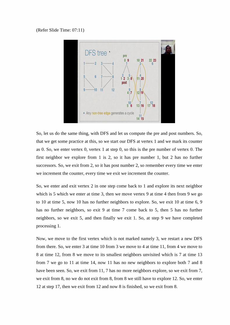
So, let us do the same thing, with DFS and let us compute the pre and post numbers. So,

that we get some practice at this, so we start our DFS at vertex 1 and we mark its counter

as 0. So, we enter vertex 0, vertex 1 at step 0, so this is the pre number of vertex 0. The

first neighbor we explore from 1 is 2, so it has pre number 1, but 2 has no further

successors. So, we exit from 2, so it has post number 2, so remember every time we enter

we increment the counter, every time we exit we increment the counter.

So, we enter and exit vertex 2 in one step come back to 1 and explore its next neighbor

which is 5 which we enter at time 3, then we move vertex 9 at time 4 then from 9 we go

to 10 at time 5, now 10 has no further neighbors to explore. So, we exit 10 at time 6, 9

has no further neighbors, so exit 9 at time 7 come back to 5, then 5 has no further

neighbors, so we exit 5, and then finally we exit 1. So, at step 9 we have completed

processing 1.

Now, we move to the first vertex which is not marked namely 3, we restart a new DFS

from there. So, we enter 3 at time 10 from 3 we move to 4 at time 11, from 4 we move to

8 at time 12, from 8 we move to its smallest neighbors unvisited which is 7 at time 13

from 7 we go to 11 at time 14, now 11 has no new neighbors to explore both 7 and 8

have been seen. So, we exit from 11, 7 has no more neighbors explore, so we exit from 7,

we exit from 8, no we do not exit from 8, from 8 we still have to explore 12. So, we enter

12 at step 17, then we exit from 12 and now 8 is finished, so we exit from 8.

Now, we come back to 4, 4 obviously, has no other vertices, so we come back to 3 and

finally, we exit from 3 at time 21 at this point 6 is still not marked. So, we start a new

DFS from 6, so we enter 6 at time 22 but 6 has no new neighbors, so we exit from 6 at

time 23. So, this like BFS generates a collection of trees. So, when we do DFS on a

disconnected graph, each connected component will generated tree.

Now, if we look at the edges which we did not explore, these will again be the edges

which are outside the tree. So, we can draw them in a different color, so we have the

edge between 5 and 10 which we did not explore, because we explored 10 directly from

9 and so on. So, once again just like in BFS, once we have finished DFS if there are non

tree edges, then we have a cycle. So, both BFS and DFS on an undirected graph can

reveal a cycle through the presence of a non tree edge.


So, the situation with directed graphs is a little more complicated, so let us see what

happens when we have cycles in directed graphs. So, in a directed graph we need to

follow the edge arrows, arrows along the edges. So, for example, 1, 3, 4, 1 is cycle,

because we can go around without changing direction, whereas 1, 6, 2, 1 is not a cycle,

because on the way back I have to switch directions from 2 to 1 which I cannot do. So,

let us do a DFS and see what this can tells us about cycles in this graph.

So, we begin with vertex 1 as usual, so 1 has pre number 0 its smallest neighbor is 2 and

the smallest neighbor of 2 is 5, and the smallest neighbor of 5 is 6, and the smallest

neighbor of 6 is 7, now from 7 that are no outgoing edges. So, we back track to 6 from 6

the only node that we can go to is 2 which have seen before, so we leave at 6. Now, we

come to 5, 5 still has an outgoing edge which is 8, so we come to 8.

Now, from 8 we cannot do anything, so we return from 8 back to 5, now 5 has nothing

left to explore. So, we leave 5 likewise we leave 2 finally, we come back to 1, now at 1

we have explored this left path. So, now we can... we do not look there we look at other

direction we go to 3. So, we explore 3, 3 will explore 4, but 4 cannot go to 8 or 1,

because 1 has already been seen and so is 8, so 4 will exit, so 3 will exit and then 1 will

exit.

So, this happens to be a single connected graph, but it has cycles, so now if we first look

at these edges, the edges that we have drawn are tree edges as before. Now, if you look at

the edges that have not been part of the tree, they fall into 3 groups. So, the first type of

edge which is not a part of the tree is what we call a forward edge, so a forward edge is

an edge which goes form a node to a node below it in the tree. So, we have a node from 1

to 6 for example,. So, this edge is a tree edge is not a tree edge, but it is a forward edge

because 1 was above 6 in the tree.

Likewise the node from 5 to 7, because we actually explore this graph as 5, 6, 7, so 5 to 7

is not tree edge. So, these are forward edges, the other category of edges which are there

in the graph which are not in the tree are backward edges, they go up the tree. So, from 6

there is this edge back to 2 which we did not use, because 2 had already been explored.

Likewise from 4 back to 1 there is this edge we did not explore, because that was already

there.

There is another category of edges which are not there in the tree, but which are there in

the graph and these are edges such as from 6 back to 2. So, this is an edge from a later

vertex to an earlier vertex or from 4 back to 1, so these are what are called back edges.

So, back edge is an edge in the graph which in the DFS tree goes from a lower vertex to

a higher vertex. And finally, there are some edges which are neither going forward nor

backward, but sideways. So, these are edges like 8 to 7 and from 4 to 8, so these cross, so

4 is not below 8 nor is 8 below 4, 7 is not below 8 because they are both below 5 and so

on.

So, these we call cross edges, now it is easy to argue that a cross edge will only go from

right to left. In other words, it can only go from higher number to lower number, because

if you wanted to draw an edge like this for instance, then this would mean that there was

an edge from 2 to 4. So, we would explore 4 through 2 rather than wait and go back 1

and explore. So, we cannot have cross edges which go from lower numbers to higher

numbers, it must go from higher numbers to lower numbers.

So, now we have not one, but 3 types of non tree edges, unlike the directed case when we

had the clear distinction between tree edges and non tree edges, here we have 3 types of

non tree edges. Now, which ones of these correspond to cycles, so if I look at this (1,3)

edge, so this (1,6) edge. So, this (1,6) edge does not actually create a cycle, because we

already saw that this is not a cycle.

So, in order for it to complete a cycle, it must be the case that there is a path including

the edge which forms a directed cycle. Now, it is easy to see that the only situation where

this will actually happen is if there is a back edge, because when there is a back edge we

know that there is a path coming from 2 down to 6 and then by following the back edge

this forms a directed cycle.

Likewise, we know that there is a path coming from 1 down to 4 by following this back

edge we form a directed cycle. On the other hand, if we look at the other types of edges

for instance, then we have this path here for this is parallel to the other path here. So,

together these are both two different ways of going from 1 to 6, but they are not a cycle,

in same way we can see that if we have a cross edge like this, then we have some path

coming from here and some path going from there.

But, again they are just two different ways of reaching 7 from 5 and they are not really a

cycle. So, in terms of... by a little analysis that only back edges form cycles and this is

actually something that you can prove we will not prove it formally, but it is argued the

way we did just now.


But, a directed graph has a cycle if and only if DFS will reveals a back edge, now it turns

out that these pre and post numberings are very useful to help as classify the types of

edges that are there in the graph. So, for both tree and forward edges, so you will notice

that if you go back to this numbering that these things form an interval that you can think

of this as from 0 to 15, from step 0 to 15 I was exploring 1, from step 11 to 14 I was

exploring 3 from step 2 to 9, I was exploring 5 and so on.

So, if you look at the pre and the post number it says I started exploring the number at

the pre and I finished exploring at post and everything else that was below happened in

between. So, for a forward edge the internal above will be bigger than the interval below.

Because, I went below during this period I came back before it ended. So, for instance

the forward edge from (0,15) to (3,6). So, the interval (3,6) is inside (0,15) this is also

true for tree edges, because in a tree edge also if I am going the forwards I enter then

lower node after I enter this. So, its starting point will be later and its ending point will

be earlier.


So, for both tree edges and forward edges, if I am going from u to v then the interval

with the start node u will contain the other one. So, this will be sitting inside this one,

(pre[v],post[v]) will be sitting inside (pre[u],post[u]), so I will have this picture. So, this

is the internal for u and this is the interval for v. Conversely it is exactly the opposite for

backward edges I start from a smaller interval and I go to a bigger interval. So, the

smaller integral will be the starting point of the edge, then the bigger integral will be the

ending point.

So, if I look at an edge in my DFS tree and if I look at the pre and post numbers

associated with the end points I can determine whether it is forward edge or backward

edge and finally, it will turn out that for cross edges the intervals are disjoint. So, we can

see here that we have finished processing 4... vertex 7 before we get to 8. So, there is no

intersection between the interval (7,8) and (4,5) likewise we have finished processing 8

before we went to 4 that is why it is a cross edge, they are on different branches of the

tree.

So, there is no intersection (7,8) and (12,13), so therefore a directed graph has a cycle if

only if DFS reveals a back edge, and we can classify edges as being forward edges,

backward edges or cross edges by just looking at the pre and post numbering of the end

points of the edge.


Now, it is important to identify cycles, because if we do not have cycles we have a very

nice class of graphs called directed acyclic graphs. These are useful for modeling

dependencies. For instance if you want to list out a bunch of courses which are being

offered and they have prerequisites, then a natural way to model this is using a directed

graph where the edges represent prerequisites, for instance if they have an edge from

algebra to calculus it indicates algebra is a prerequisite for calculus, it will not have

cycles.

Because we cannot have two courses which are prerequisites for each other; otherwise,

we will not be able to take either course. So, we will look at directed acyclic graphs or

DAGs soon in a later lecture.


What about connectivity in directed graphs? So connectivity in a directed graph is not

just a question of having these edges between the graphs, but having them in the right

direction. So, we say that two nodes are strongly connected, if I can go from i to j by a

path and I can come back from j to i by a path. So, it is not enough to just have edges in

some haphazard direction I must be able to go from i to j and come back from j to i in

which case I say that it is strongly connected.

So, it turns out that a directed graph can always be decomposed into what are called

strongly connected components. A strongly connected component has a property that

every pair of nodes in that component is strongly connected from every node in the

component you can go to every other node in the component and come back.


So, for instance if will look at this graph then strongly connected components, one is the

cycle 1, 3, 4 we can go from 1, 2, 3 to 4 and come back. So, from any node in this cycle

we can come back to any other node. Likewise 2, 5 and 6 forms are strongly connected

component, 7 on its own is a strongly connected component. Because, we cannot go

anywhere and 8 also is a strongly connected component, because if we leave 8 we cannot

come back to 8 the way this graphic is structured.

So, this graph has 4 strongly connected components, now it turns out that DFS

numbering using pre and post numbers can be used compute strongly connect

components a very elegant algorithm is given in the book by Dasgupta Papadimitriou

and Vazirani and if you are interested you can look it up in that book.


So, we have seen some concrete examples of what you can compute, there are many

other properties that you can compute using BFS and DFS. For instance, there are these

things called articulation points, if you your graph looks like this where I have some

vertex which is a crucial vertex, if I remove this vertex this graph falls apart into

disconnect components, I can identify such vertices using BFS and DFS in particular

using DFS.

Similarly, if I have a situation where I have an edge like this, where if I remove this edge

then the graph gets disconnected, then I can again identify such an edge using DFS.

Now, these are important, because if these represents some kind of communication

network or some road network, in these are bottle necks, these are critical points, if this

is an intersection and there is an accident no traffic and go from any part on the left to

any part on the right or if this is a network if this cable gets cut then the network will get

cut disconnected into components.

So, these kinds of properties can also be computed during BFS and DFS. So, it is

important to realize therefore, that BFS and DFS is not just for connectivity, to finding

out whether vertex s can reach vertex t, you can get a wealth of information and these are

linear time algorithms and these are all operations which can be performed during BFS

and DFS. So, very efficiently you can compute various properties of the graph and use

these to exploit these to design more efficient procedures or to identify other things that

need to be done.

Design and Analysis of Algorithms Prof. Madhavan...

Documents

Transcript of Design and Analysis of Algorithms Prof. Madhavan...