NAG-2001

Design and Analysis of a 6U CubeSat and Mission

A Major Qualifying Project Report Submitted to the Faculty of the

WORCESTER POLYTECHNIC INSTITUTE in Partial Fulfillment of the Requirements for the

Degree of Bachelor of Science in Aerospace Engineering

by

_____________________ Tristan Andreani

_____________________ Samuel Joy

_____________________ Edward J. Beerbower

_____________________ Benjamin Snyder

_____________________ Roberto Clavijo

_____________________ Jeremiah Valero

_____________________ Gavin Lee

April 6, 2020

Approved by

_________________________________ Nikolaos A. Gatsonis, Advisor

Professor, Aerospace Engineering Program

_________________________________ Zachary R. Taillefer, Co-Advisor

Assistant Teaching Professor, Aerospace Engineering Program

2

Abstract

This project presents design and analysis for a 6-unit CubeSat carrying a miniaturized mass

spectrometer. The CubeSat is inserted at the International Space Station (ISS) altitude and uses the

BET-300-P electrospray thruster to acquire an orbit with perigee at about 200 km and apogee at

440 km.Orbital analysis using the SystemsToolKit (STK) provides an orbital life of about 45 days.

STK simulations estimate 17 W of available power and battery capacity of 40 Wh, STK

simulations provide the downlink transfer periods with the Near Earth Network and the thermal

fluxes onto the CubeSat. COMSOL Multiphysics simulations determine that the induced magnetic

fields from the magnetorquers do not adversely affect electronics and sensors.Preliminary design

of a thermal vacuum chamber is also presented.

“Certain materials are included under the fair use exemption of the U.S. Copyright Law and

have been prepared according to the fair use guidelines and are restricted from further use."

3

Acknowledgements

We would like to thank the following individuals for their help, support, and contributions to

this project.

Project Advisors Professor Gatsonis Professor Taillefer

Graduate Student Advisors Harrison Hertlein

Academic & Research Computing Advisors Adriana Hera

Structural Design Team Professor Karanjgaokar (Advisor) Brian Kelsey Nicole Petilli Christian Anderson Rory Cuerdon

Attitude Determination and Controls Team Professor Demetriou (Advisor) Oliver Hassan Chris Renfro David Resmini Andrew Montero Robaire Galliath

4

Table of Authorship

Introduction

Background and Literature Review

CubeSat Applications and Missions Andreani

Review of CubeSat MQPs at WPI Joy

Project Goals All

Design Requirements

Power Lee

Propulsion and Orbital Parameters Snyder, Valero

Telecommunications Beerbower

Environmental Effects Clavijo

Overall Project Management Joy

MQP Objectives, Methods, and Standards All

MQP Tasks and Timetable Joy

Payload and Design Implications Joy

Propulsion Design and Analysis Snyder, Valero

Power Subsystem Design and Analysis Lee, Andreani

Telecommunications Design and Analysis Beerbower

Environmental Effects Analysis Clavijo, Joy

Thermal Vacuum Chamber Preliminary Research

Andreani

Conclusions and Recommendations All

Social Impacts Andreani

5

Table of Contents

Abstract ..................................................................................................................................... 2 Acknowledgements ................................................................................................................... 3 Table of Authorship .................................................................................................................. 4 Table of Contents ...................................................................................................................... 5 Table of Figures ........................................................................................................................ 8 List of Tables .......................................................................................................................... 10 1. Introduction ................................................................................................................... 11

1.1 Background and Literature Review .............................................................................. 12 1.1.1 CubeSat Applications and Missions ...................................................................... 12 1.1.2 Review of CubeSats at WPI ................................................................................... 14

1.2 Project Goals ................................................................................................................. 15 1.3 Design Requirements, Constraints, and Other Considerations ..................................... 17

1.3.1 Propulsion and Orbital Parameters ........................................................................ 17 1.3.2 Power ..................................................................................................................... 19 1.3.3 Telecommunications .............................................................................................. 20 1.3.4 Environmental Effects............................................................................................ 21

1.4 Overall Project Management and Budget ..................................................................... 22 1.5 MQP Objectives, Methods, and Standards ................................................................... 23 1.6 MQP Tasks and Timetable ........................................................................................... 25

2. Payload and Design Implications.................................................................................. 27 2.1 Payload Overview ......................................................................................................... 27 2.2 Consideration of CubeSat Design Criteria .................................................................... 29 2.3 Determination of Data Collection Period ..................................................................... 30

3. Propulsion Design and Analysis ................................................................................... 33 3.1 Propulsion Overview .................................................................................................... 33 3.2 Busek Electrospray Thruster (BET) ............................................................................. 33 3.3 Phase III Analysis and Results...................................................................................... 34

3.3.1 Orbital Transfer Results ......................................................................................... 37 3.4 Phase 4 Analysis and Results........................................................................................ 43

4. Power Subsystem Design .................................................................................................... 48 4.1 Power Subsystem Overview ......................................................................................... 48

4.1.1 CubeSat Power Budget .......................................................................................... 49

6

4.1.2 Power Subsystem Hardware .................................................................................. 50 4.2 Power System Evaluation ............................................................................................. 54 4.3 Power Component Selection ......................................................................................... 54 4.4 Power Profile Modeling ................................................................................................ 55 4.5 Power Subsystem Results ............................................................................................. 60

4.5.1 Final Hardware Configurations .............................................................................. 60 4.5.2 Power Profile Results ............................................................................................. 62

5. Telecommunications Analysis ............................................................................................ 69 5.1 Telecommunications Overview .................................................................................... 69

5.1.1 Coverage ................................................................................................................ 70 5.1.2 Transceiver ............................................................................................................. 71 5.1.3 Antenna .................................................................................................................. 72

5.2 Hardware Selection ....................................................................................................... 72 5.2.1 Transceiver ............................................................................................................. 73 5.2.3 Antenna .................................................................................................................. 74

5.3 Coverage Estimates ....................................................................................................... 76 5.4 Telecommunications Results ........................................................................................ 78

6. Environmental Effects Analysis ......................................................................................... 79 6.1 Environmental Effects Overview .................................................................................. 79 6.2 Environmental Effects Research ................................................................................... 80 6.3 Modeling Atmospheric Effects ..................................................................................... 81 6.4 Magnetic Interference Modeling .................................................................................. 83

6.4.1 Modeling a Single Magnetorquer .......................................................................... 84 6.4.2 Modeling the Earth’s Background Magnetic Field ................................................ 86

7. Thermal Vacuum Chamber Preliminary Research ............................................................. 88 7.1 Testing Applications and Standards ............................................................................. 88

8. Conclusions, Recommendations, and Social Impacts......................................................... 90 8.1 Payload Summary ......................................................................................................... 90 8.2 Propulsion and Orbital Analysis ................................................................................... 90 8.3 Power Analysis ............................................................................................................. 91 8.4 Telecommunications Analysis ...................................................................................... 91 8.5 Environmental Effects Analysis ................................................................................... 91 8.6 Recommendations ......................................................................................................... 92

2. Payload ........................................................................................................................ 92

7

3. Propulsion ................................................................................................................... 92 5. Telecommunications ................................................................................................... 93 6. Environmental Effects ................................................................................................ 93

8.7 Social Impacts of CubeSats .......................................................................................... 94 Works Cited ............................................................................................................................ 97 Appendices ............................................................................................................................ 103

Appendix A: Battery Charge Code ................................................................................... 103 Appendix B: Sample STK Data for Battery Charge ......................................................... 108

8

Table of Figures

Figure 1 - Isometric View of the NAG-2001 CubeSat, NeAtO .................................................... 12

Figure 2 - Gantt Chart for the project ........................................................................................... 26

Figure 3 - The miniNIMS used aboard the Dellingr 6U (NASA, 2017) ...................................... 27

Figure 4 - Activation Altitude vs. Data Collected Per Orbit......................................................... 32

Figure 5 - Overview of the low-thrust orbital transfer .................................................................. 36

Figure 6 - Engine Model defined in Component Browser ............................................................ 38

Figure 7 - Thruster Attitude, Engine and Propagator ................................................................... 39

Figure 8 - Thruster Attitude, Engine and Propagator ................................................................... 40

Figure 9 - Stopping Conditions for Orbital Transfer STK ............................................................ 41

Figure 10 - Graph Showing Orbital Motion of NeATo ................................................................ 42

Figure 11 - Image Showing NeATo Iterations Around the Globe................................................ 43

Figure 12 - Altitude over five orbital periods ............................................................................... 45

Figure 13 - Altitude vs. Orbital periods; low thrust example ....................................................... 46

Figure 14 - Altitude vs. Orbital periods; high thrust example ...................................................... 47

Figure 15 - Altitude vs Orbital Periods for Optimal Orbit............................................................ 47

Figure 16 - EPS power distribution (Kalde, 2012) ....................................................................... 52

Figure 17 - Example of parented solar panels and cells in Blender.............................................. 56

Figure 18 - Edits to be made in Blender-created 3D Cubesat Model .dae and .anc files (AGI Inc.)....................................................................................................................................................... 57

Figure 19 - A direct example of edits made in a Blender-created 3D CubeSat Model .dae file .. 58

Figure 20 - Sun-synchronous power generation of a 6U ram-facing NeAtO ............................... 58

Figure 21 - NeAtO early power generation over a single day ...................................................... 62

Figure 22 - NeAtO early power generation over 150 days ........................................................... 63

Figure 23 - Final power generation over a single day .................................................................. 65

Figure 24 - Final power generation over 150 days ....................................................................... 65

Figure 25 - Battery charge over a single day ................................................................................ 66

Figure 26 - Battery charge over 150 days ..................................................................................... 66

Figure 27 - NeAtO's altitude and power generation over a single day early in the mission ......... 67

Figure 28 - NeAtO's altitude and power generation over a single day later in its lifetime ........... 67

Figure 29 - NASA NEN stations with coverage zones (NASA, STK) ......................................... 70

Figure 30 - VHF/UHF Duplex Transceiver (ISISpace) ................................................................ 71

Figure 31 - Access periods to ground station network ................................................................. 78

9

Figure 32 - NeAtO External Temperature Versus Solar Intensity ................................................ 82

Figure 33 - NeAtO's Thermal Profile from COMSOL ................................................................. 83

Figure 34 - Magnetic flux density in single magnetorquer ........................................................... 85

Figure 35 - Magnetic field lines inside single magnetorquer ....................................................... 85

Figure 36 - Magnetic Flux Density vs. Distance Along the Z-Axis ............................................. 86

Figure 37 - Defeatured CubeSat skeleton in COMSOL ............................................................... 87

10

List of Tables

Table 1 – Busek Electrospray Thruster Specifications ................................................................. 34

Table 2 - Parameters used in STK propellant budget simulation ................................................. 36

Table 3 – Constant parameters for elliptical orbit code ................................................................ 44

Table 4 - Final Power Budget of the 2018 CubeSat for eLEO MQP (JB3-1801, 2018) .............. 49

Table 5 - NeAtO's final power budget .......................................................................................... 64

Table 6 - Transceiver and Transmitter Comparison ..................................................................... 74

Table 7 - Transceiver and Transmitter Comparison ..................................................................... 75

Table 8 - STK Scenario Orbit Parameters .................................................................................... 76

Table 9 - Ground Station Coordinates .......................................................................................... 77

Table 10 - Constants for determination of turns in magnetorquer coil ......................................... 84

11

1. Introduction

CubeSats are small, cost effective satellites which expand commercial access to space. Defined

by the standardized Unit (a cube with dimensions of 10cm x 10cm x 10cm, ~1.3kg, denoted 'U'),

CubeSats are typically 1U, 2U, 3U, 6U, or 12U. Each Unit is composed of hardware components

specifically selected to complete the satellite's mission. The concept began in 2000 as a plan to

provide scientific and military laboratories another tool to grow their operations in space. Many

colleges and high schools have programs that allow students to design and build their own

CubeSats, illustrating that the concept lends itself to valuable educational experience. (Loff, 2015)

This MQP group, alongside its partner MQPs MAD-2001 (Galliath, R., Hasson, O., et al.,

2020) and NK-2001 (Anderson, C., Cuerdon, R., et al., 2020), is part of a Systems Engineering

Group (SEG) with an overall project goal to perform the conceptual design of a 6U CubeSat. The

NIMS eLEO (extreme Low Earth Orbit) Atmospheric Observer (NeAtO) CubeSat is designed to

carry a miniaturized Neutral Mass and Ion Spectrometer (NIMS), a proprietary scientific

instrument from NASA Goddard for the purpose of scientific experimentation and data collection

in the ionosphere (Gatsonis, N.A., Ye, L., et al., 2019).

A solid model of NeAtO is shown in Figure 1. Designed for deployment from the International

Space Station (ISS) via NanoRacks at 400km with a 51.6o inclination, the satellite then enters a

200-440km elliptical orbit via a low thrust transfer, maintaining a perigee within eLEO for

approximately 150 days. The goal of this MQP is to design and analyze the propulsion,

telecommunications, power subsystems, perform payload integration, and perform orbital and

environment effects analysis.

12

Figure 1 - Isometric View of the NAG-2001 CubeSat, NeAtO

1.1 Background and Literature Review

The following section provides relevant background information and mission objectives. A

brief history of CubeSats and their scientific relevance is followed by an overview of previous

projects done by Worcester Polytechnic Institute (WPI). The section is concluded by introducing

the goals this mission aims to complete for this project.

1.1.1 CubeSat Applications and Missions

In recent years, the CubeSat has become a unique tool in the scientific community. A

cooperative culture has formed around the implementation of CubeSats into everyday space

science. NASA's CubeSat Launch Initiative (CSLI) provides opportunities to launch small

satellites aboard larger launch vehicles as secondary payloads. The industry consists of companies

(e.g. Clyde Space, ISIS) providing interested parties with components necessary to construct the

satellite, who then work with integration services (NanoRacks, SpaceFlight Services, etc.) to

facilitate the satellite's flight aboard a launch vehicle (Loff, 2015).

13

CubeSats are currently experiencing rapid growth in popularity and technological opportunity.

The main advantage to using CubeSats is due to their small size, flexibility of platform design, and

simplicity of internal components. Being constrained to discrete sizing of 10cm x 10cm x 10cm

units turns the CubeSat into a uniform template for which companies can design consumer off-

the-shelf (COTS) parts. This means, if a small scientific payload can be built to fit into a CubeSat,

the subsequent mission planning and subsystem creation can be tailored to the payload's

requirements. Since 2013, NASA has arranged for 14 CubeSat missions, which utilize their

flexibility and design freedom; examples include the Radiometer Atmospheric CubeSat

Experiment (RACE) and Interplanetary Nan-Spacecraft Pathfinder In Relevant Environment

(INSPIRE). RACE monitors the Earth's water vapor and INSPIRE is a dual-CubeSat

communication chain from Mars to Earth that demonstrates CubeSat operation, communication,

and navigation in deep space. Once CubeSat operation in deep space has been successfully

demonstrated with INSPIRE, their utility can then extend to third viewpoint observations,

advanced reconnoitering of exploration sites, and remote monitoring of other missions (JPL:

NASA, n.d).

The global CubeSat market was estimated to have a value of $152 million in 2018, which is

projected to rise to nearly $375 million. The coming years expect reduced mission costs, a greater

demand for data from Earth observation in LEO, and increased opportunity in government,

military, and commercial applications (Markets and Markets, n.d). While the future of CubeSats

appears to hold countless possibilities, one of their greatest applications is expanding the academic

realm with hands-on mission planning and spacecraft design.

14

1.1.2 Review of CubeSats at WPI

There are several prior MQPs at WPI which focused on CubeSat development. The 2017 MQP

CubeSat project “Design and Analysis of the Sphinx-NG CubeSat” (NAG-1701, 2017; MAD-

1701; 2017; JB3-1701, 2017) designed a 3U CubeSat with a mission of observing space weather.

The SphinX-NG instrument, developed by the Space Research Center in Warsaw, Poland,

performed the observations of space weather. This payload monitored the x-rays of long-term solar

flux variability, investigated solar features such as inactive coronas, active regions, solar flares,

and plasma irregularities, and observed terrestrial gamma-ray flashes, auroral x-ray spectra, and

orbital particle fluctuations. This project in turn expanded upon the work of the 2012 and 2013

MQPs which utilized the same instrument. Their CubeSat was designed to be deployed into a

circular polar orbit of 600km, and achieved a lifespan of 17.8 years, which would allow the

SphinX-NG instrument to perform its scientific duties and provide more than sufficient data

collection through such a long lifetime (NAG-1701, 2017).

The 2018 MQP CubeSat project (NAG-1801, 2018; MAD-1801, 2018; JB3-1801, 2018)

created two designs for two different objectives. The first part of their mission was to evaluate the

feasibility and duration of flights in eLEO (approximately 210km altitude). This team determined

a 3U configuration could not successfully produce enough power, instead opting for a custom 4U

frame to accommodate enough solar panels (NAG-1801, 2018). Additionally, despite not reaching

its desired 90-day orbit, the team succeeded in obtaining a 24-day lifespan and analyzing the effects

of eLEO over that duration (NAG-1801, 2018). The second part of the 2018 mission was to test

the possibility of maintaining a 100km arc distance between two CubeSats. Achieving this goal

would support the ability to use several small satellites rather than a single large one, which would

make it easier to replace malfunctioning components and reduce the operation cost. There was no

15

real conclusion as to whether or not this rendezvous operation could be successfully completed

(NAG-1801, 2018).

In addition to MQPs, research at WPI has been extensive (Moorthy et al, 2019; Moorthy et al,

2018; Kewen et al, 2017; Blandino et al, 2016; Gatsonis et al, 2016). The work of Moorthy et al.

(2018; 2019) presented the use of the Busek Electrospray Thruster on orbital analysis to extend

the lifetime of a Cubesat in extreme LEO orbit. The following list provides the additional sources

for CubeSat research originated from WPI.

1.2 Project Goals

This scientific mission uses a mass spectrometer, within a 6U CubeSat (NeAtO) platform,

orbiting with perigee in eLEO. Throughout NeAtO's lifetime, the miniaturized NIMS payload will

collect data on atmospheric composition in the ionosphere and relay that data to Earth for analysis.

The data will be used to analyze atmospheric weather patterns in order to predict the impacts of

geomagnetic storms, and to better understand atmospheric irregularities which affect global

communications (NASA, 2017). The planned orbit is an elliptical orbit achieved after ISS

deployment, with a perigee of about 200 km and an apogee of about 440 km. The major objective

of the mission is to maximize the lifespan of NeAtO due to its extended eLEO by modifying orbital

parameters and maximizing fuel efficiency of the onboard propulsion system. The desired mission

lifespan is 150 days, which will provide the payload the opportunity to capture data across all

seasons on Earth.

This project will provide the soft design, supported by analysis, of the NeAtO spacecraft.

NeAtO will execute measurements of the atmospheric composition in the ionosphere using the

miniaturized NIMS payload. NeAtO will control payload data collection, storage and downlink,

16

as well as maintain the slightly elliptical orbit required to interrogate the ionosphere. The data will

be used to analyze atmospheric weather patterns in order to predict the impacts of geomagnetic

storms, and better understand atmospheric irregularities, which affect global communications

(NASA, 2017).

The overall mission has several phases; deployment from the ISS (Phase I), detumbling (Phase

II), orbit transfer (Phase III) and science (Phase IV). In Phase I, NeAtO will be deployed from the

ISS which has a circular orbit at a 410km altitude and an inclination of 51.6°. Once deployed, in

Phase II, NeAtO will power on for the first time and automatically eliminate any unwanted

spacecraft rotation. Once detumbling is confirmed and communication established, Phase III will

begin and NeAtO will shape the orbit to final orbit using onboard propulsion. In Phase IV, the

spacecraft will perform measurements of the ionosphere in eLEO until the spacecraft runs out of

fuel or the orbit degrades. It will then de-orbit, as required by CubeSat mission guidelines.

The final orbit (Phase IV) is elliptical with perigee and apogee of approximately 200 km and

440 km, respectively, which will allow several layers of the ionosphere to be interrogated. The

primary mission objective is to optimize the science and data collection phase, in part, by

maximizing the residence time of NeAtO in this orbit. In this phase, NeAtO will experience a

significant drag force eLEO, which must be compensated for by the onboard propulsion system in

order to persist in eLEO. Drag compensation will extend the mission lifetime; however, the orbit

will still degrade due to the high levels of atmospheric drag at this altitude.

17

1.3 Design Requirements, Constraints, and Other Considerations

As described above, the design of NeAtO includes three distinct MQPs, each comprised of

several subsystems typical of spacecraft projects. The following section describes the

responsibilities and goals of each subsystem in this MQP team for the NeAtO spacecraft.

1.3.1 Propulsion and Orbital Parameters

The goal of the propulsion subsystem is to provide a mission profile that will allow NeAtO to

achieve its scientific mission with constraints of fuel, space and power allowed for this subsystem.

Primary propulsion is used for orbit shaping, changing and maintenance. In terms of primary

propulsion, the mission profile includes orbit shaping (Phase III) and maintenance in the science

orbit (Phase IV). Optimization of orbit shaping maneuver will determine how much propellant will

be available to maintain the science orbit, which is the primary mission objective. The Systems

Tool Kit (STK) and custom MATLAB programs for low-thrust trajectory analysis will provide

initial propellant usage estimates for these maneuvers.

As selected by the MAD2001 MQP (MAD2001, 2020), the NeAtO spacecraft will be deployed

from the ISS. As such, the initial orbit in Phase III is circular at approximately 400km, with

inclination of 51.6°. STK will provide the time, propellant and trajectory required to execute the

Phase III orbit-shaping maneuver. This analysis will determine how much propellant is available

to the spacecraft entering Phase IV, which ultimately determines how much propellant remains to

extend the science mission and de-orbit the spacecraft; a critical mission objective. Initially,

continuous thrust along the velocity vector will be assumed. This analysis may be refined, at which

time thruster commands would be relayed to the ADC subsystem team.

18

The MATLAB program will be used to perform the trajectory analysis for the Phase IV orbit,

which includes regions where the spacecraft will experience significant drag. This analysis will

provide parameters required by the OBC, which include thruster throttle level, firing sequences

and firing durations. Several parameters can be adjusted including apogee and perigee, thrust

levels, wet and dry masses, specific impulse, drag coefficients, and many others which affect the

propellant usage and thruster firing sequence. Optimization of this orbit will be critical to

extending mission life in this phase of the mission.

In order to design and optimize the orbital profiles and maneuvers, several constraints that limit

the analysis and propulsion subsystem must be addressed. The first constraint is the small mass

and volume of the satellite. To maximize mission lifetime with such a small propellant budget, it

is important to avoid any unnecessary maneuvers, especially particularly propellant-heavy ones

such as inclination changes. Performing a significant orbit transfer or inclination change requires

a large portion of the available propellant, which is impractical and should be avoided when the

mission objective does not require it. The second constraint is the significant drag experienced by

the spacecraft at eLEO altitudes. This constraint requires optimizing the desired perigee and

apogee with fuel requirements in order to maximize mission lifetime and minimize fuel

consumption in the orbit transfer and maintenance. The third constraint is the available power

throughout the mission. Many of the spacecraft components will require power at various stages

of the mission and orbit. The available power, as determined by the power subsystem, will

influence onboard propulsion system firing sequences and could impact propellant usage and

optimization.

19

1.3.2 Power

The power subsystem consists of three main elements: the hardware to generate, store, and

distribute electrical power; a power budget to manage and distribute the power; and a

generation/capacity timeline to support the power draw of the CubeSat throughout the mission.

These tasks are interconnected; making progress in one allows for progress in another. Selecting

effective hardware will lead to creating a system that can generate enough power to follow the

desired power budget.

An initial power budget provides an estimate of how much power each component will draw

at various points in the orbit. This first budget guides an initial hardware selection, from which a

power profile is created and analyzed. A functioning subsystem consists of hardware that procures

a power profile which satisfies the power budget. Should the selected hardware not create a

sufficient profile, adjustments must be made to both the budget and the hardware until the

subsystem can fully support the mission.

The power requirements of other subsystems can thus constrain the power subsystem: the

summation of many components' minimum power draw throughout the mission sets a minimum

required power generation. Hardware selection is also constrained, as what is available on the

market may not satisfy the power demands of the satellite. The ideal piece of hardware will not

exist, and so the system must be designed in a way to optimize its performance. While some of the

NeAtO’s components can be managed to only draw power when absolutely needed, many

components must operate at certain power levels at certain times, limiting how much the power

budget can be optimized.

20

1.3.3 Telecommunications

The telecommunication subsystem provides satellites with a way to send and receive data. For

spacecraft similarly sized to NeAtO, it is not feasible to store data on the payload and the onboard

computer until it can be downlinked, nor is it possible to have a downlink network able to

continuously receive the data. Thus, it is important to have a system that can effectively provide

long downlink periods for the payload's collected data, and transmit this data as fast as can be

supported. The mission will only provide useful data as it can be downlinked. The main constraint

for the telecommunications subsystem is its power usage. As telecommunications does not directly

affect mission lifespan, it would be one of the first subsystems to have its power budget reduced.

Limiting the power rate of the subsystem means that the components would operate at lower rates,

slowing the speed of data transmission. The ideal optimized telecommunications system sends and

receives all relevant information within its access period with the Ground Station Network.

The physical subsystem consists of two components: an antenna, and a signal processing

device. The signal processor may be either a transmitter and receiver working together, or a

transceiver, which is the two combined into one component. A consideration for the hardware is

the frequency of signals it will generate and receive. Higher frequencies can transmit data faster

but require more power and more robust hardware (Beasly, 2014). The physical constraints on the

telecommunication subsystem are shared with the rest of the CubeSat systems; it must take up

minimal space internally, add as little weight as possible to the spacecraft, and not obstruct

instruments that operate externally.

21

1.3.4 Environmental Effects

Extreme Low Earth Orbits (eLEO) are complicated because of their dense atmosphere, high

thermal loading, and strong magnetic interference with spacecraft components. Low altitude orbits

induce higher levels of drag that will add to the overall vehicle temperature of NeAtO. Adding a

heat shield to protect against drag induced heat will not solve all the issues presented by a space

environment. Ionized oxygen and thermal radiation from the sun require that the spacecraft

structural material must be treated so the aluminum material does not deform or melt. In addition,

the components that make up NeAtO must remain within operating temperatures throughout the

mission. Even if all components and materials can withstand the space environment, another

physical constraint on NeAtO is thermal shock. Thermal shock refers to a quick fluctuation of

temperature. The temperature change adds structural stress on each individual component and

material in a CubeSat. Each material has a coefficient of thermal expansion (CTE), thus each

component will expand and contract at a different rate. This difference can lead to electronic failure

even if the components remain in operating temperature range.

Magnetic interference, from the Earth’s magnetic field or other sources, can possibly affect the

attitude control system and other components. Magnetometers determine the magnetic field

strength of the Earth relative to its own coordinate system, predict inbound field vectors, and

compute the attitude control inputs required to align the spacecraft with the desired orientation.

The spacecraft is reoriented via magnetorquers, electromagnetic rods which produce a magnetic

moment against the Earth’s background magnetic field. If the magnetic field created by the

magnetorquers exceeds the magnetometer’s error tolerance, then proper shielding measures must

be taken to mitigate interference. Additionally, the magnetorquers cannot be placed too close to

electrically-sensitive components such as the onboard computer and the payload’s electronic

22

components, otherwise any internal data storage may be corrupted by the resultant magnetic force.

As a result, the strength of the field generated by a single magnetorquer must be determined via

computer simulation (using the COMSOL Multiphysics modeling software) in order to provide

the Structures team with any constraints on magnetorquer position. Otherwise, magnetic shielding

for sensitive components must be considered.

1.4 Overall Project Management and Budget

The NEAtO project consists of three separate MQP teams, each responsible for different

aspects of the project as follows:

● Thermal and Mechanical Subsystems and Analysis overseen by MQP NK-2001

(NK1-2001, 2020).

● Attitude Determination and Control overseen by MQP MAD-2001 (MAD-2001,

2020).

● Payload, Propulsion, Power, and Telecommunication Subsystems, as well as

Environmental and Orbital Analyses, overseen by MQP NAG-2001.

Each week, the three MQP groups and their advisors met as one Systems Engineering Group

(SEG). At these meetings, one member from each MQP team would present the progress their

team made within their subsystems and the open issues which had come up over the past week.

The MQP advisors and other teams were encouraged to ask questions and comment to clarify any

incorrect or uncertain points. The meetings were also used to request, address, and complete open

issues.

23

1.5 MQP Objectives, Methods, and Standards

1. Perform Payload Integration

a) Evaluate when in the orbit the payload turns on and off for its data-collecting intervals.

b) Determine the necessary power and telemetry budget to complete the primary mission.

c) Plan mission operations for the entire life cycle from deployment to deorbiting in order to

ensure all subsystems function toward completing the mission objectives.

d) Properly interface the payload with the spacecraft and connect it to the onboard computer.

2. Perform Orbital Analysis

a) Determine the propellant required to transfer from the initial orbit to the desired elliptical

orbit

b) Determine the final orbit for the science phase of the mission

c) Maintain the desired orbit for as long as possible.

d) Obtain orbital parameters to analyze the solar flux on the spacecraft to determine power

draw, the drag profile on the spacecraft, and environmental effects in eLEO.

3. Propulsion Design and Analysis

a) Determine the amount of fuel and thrust required to compensate for the drag NeAtO will

experience in eLEO using the Busek electrospray thruster BET-300-P.

b) Determine the burn time necessary to optimize NeAtO's orbital lifespan to fulfill the

payload’s mission requirements.

c) Determine NeAtO's total 𝛥𝛥𝑉𝑉 and fuel consumption.

d) Determine NeAtO's final orbital lifespan.

4. Power

24

a) Create a power budget to assign the power distribution to each hardware component.

b) Select hardware and develop a power profile to satisfy the power budget.

5. Telecommunications

a) Identify a viable Ground Station Network (GSN) within the satellite's coverage range that

will maximize data transmission.

b) Select telecommunications hardware that complies with its power allowance and NeAtO's

structural requirements.

c) Establish uplink and downlink budgets for the payload and other data-handling

instruments.

6. Environmental Effects

a) Identify hazardous space agents and their influence on NeAtO's physical integrity and

operational performance.

b) Create a thermal loading model of NeAtO.

c) Create a model of the magnetic interference on internal components due to Earth's magnetic

field and due to the use of magnetorquers for attitude control.

d) Provide recommendations to protect NeAtO from the identified hazards.

25

1.6 MQP Tasks and Timetable

The Gantt Chart presented in Figure 2 outlines the timetable this MQP set to complete specific

tasks. It was used as a reference for the team's progress.

26

Figure 2 - Gantt Chart for the project

27

2. Payload and Design Implications

This chapter presents a description of the NIMS scientific payload onboard NeAtO. The

payload for a scientific mission is the main driving factor behind mission design and all other

subsystems must accommodate its requirements. These requirements, such as orbital position, data

transfer and collection, power usage, and pointing characteristics, are outlined below in order to

set a baseline for the design of the other subsystems.

2.1 Payload Overview

The payload used on this mission is a miniaturized NIMS provided by NASA Goddard Space

Flight Center Heliophysics Science Division (N. P. Paschalidis, 2019). This instrument, shown in

Figure 3, requires approximately 1.3U of NeAtO's total volume (13cm x 10cm x 9cm), and

provides in-situ measurements of atmospheric composition and density via two apertures aligned

with the velocity vector (also referred to as ram-facing), each with a 10° by 10° conical field of

view. One of the apertures is specifically dedicated to the collection of ions, while the other has a

charged screen to deflect ions and only analyze neutral particles (NASA, 2016). The following

section aims to identify notable features of the miniNIMS and how each affects the mission design.

Figure 3 - The miniNIMS used aboard the Dellingr 6U (NASA, 2017)

28

Aiming to both analyze the dynamic weather of the ionosphere as well as to determine the

steady state background atmosphere conditions (NASA, 2016), two CubeSat missions have been

launched with the miniNIMS (EXOCUBE-1, Dellingr 6U) and two more launches are scheduled

for the near future (EXOCUBE-2, PETITSat). EXOCUBE-1 was a 3U configuration sponsored by

the National Science Foundation and developed by the California Polytechnic State University

(CalPoly). Launched in January 2015 as a secondary payload aboard ELaNa-X SMAP, it achieved

a successful elliptical polar orbit of 470-600km at 98° inclination (NSF, 2013, p. 44). Its antenna

failed to deploy properly, resulting in a lower data transmission rate, but in-situ data collection was

successful (NASA, 2016). As a result, CalPoly has also developed EXOCUBE-2, which is planned

as a follow-up mission to re-attempt EXOCUBE-1, with an estimated launch date of March 15th,

2020 (NSF, 2017).

The Dellingr 6U CubeSat was developed internally by NASA to test its own payload and

attempt to build a more resilient CubeSat than most prior models (NASA, 2017). Having launched

and deployed in 2017, it has suffered numerous setbacks in orbit, including its attitude

determination and control systems and GPS (NASA, 2018), but has been able to recover from

these issues and transmit data successfully. The Plasma Enhancements in The Ionosphere-

Thermosphere Satellite (PETITSat) will launch in 2021, aiming for a lower orbit in order to explore

a regime of 80-400 km, while maintaining the same 6U frame as the Dellingr spacecraft.

Specifically, it will investigate the impact of ionospheric depletions (or “bubbles”) and

enhancements (or “blobs”) in the mid- and low-latitude ionosphere on global communications

(NASA, 2017).

29

2.2 Consideration of CubeSat Design Criteria

The payload creates many of the parameters and constraints for the mission. The payload

requires a ram-facing orientation in order to collect particles through the two apertures, which

provides a hard-set attitude to maintain. During data collection, the payload uses 1.8W of power

at full operation and collects 13.7kB of data per second, so the data collection period will need to

be adjusted to not overburden the power or telecommunications subsystems. To produce

meaningful data, the scientific goal driving this mission is to investigate the transition between the

F1 and F2 layers of the ionosphere. As such, the orbital perigee must be below the F1/F2 transition

altitude (220km), and the apogee must be balanced such that the fuel consumed to achieve the orbit

does not significantly shorten the mission lifespan but is not too low to create significant

atmospheric drag per orbit.

Before obtaining the payload specifications, the initial suggested orbit and CubeSat size was a

4U configuration - a custom frame from Clyde Space in a 1U x 1U x 4U orientation - orbiting at

250-600km. However, the payload’s dimensions are 1.3U x 0.9U x 1.0U, with the apertures on the

1.3U x 1.0U face and would limit the positioning of thrusters. This would force the payload to be

aligned with the 1U x 4U face of the CubeSat, massively increasing the expected drag per orbit.

The structures team (NK-2001) and this team met to discuss the pros and cons of a 4U versus 6U

configuration, and the 6U configuration was determined to meet every requirement for NanoRacks

deployment. This configuration will increase surface area by about 43%, allowing for more solar

panels, while increasing its internal volume, mitigating internal size constraints and providing

more flexibility for orientation of components within the 6U structure. Additionally, this allowed

a reduced surface area for drag calculations with the 2U x 1U ram-facing, all at the cost of slightly

more mass.

30

This 6U configuration (2U x 3U x 1U) allowed the payload apertures to point along the ram-

facing vector, as it is placed along the lengthwise 2U x 1U face, exactly opposite the thrusters. The

original orbit did not cross the F1/F2 threshold either, and the fuel spent for the orbital raise from

ISS deployment to a 600km apogee reduced the mission lifespan to 61 days. A new orbit, 200-

440km after ISS deployment, was proposed to counteract these two issues, and was analyzed by

the orbital analysis and propulsion subsystem teams to improve mission lifespan while allowing

the desired data to be captured.

2.3 Determination of Data Collection Period

The NIMS collects data at 13.7kbps uncompressed at the fastest sample rate of 0.1

seconds/sample and with 1.8W of power. NeAtO will use this instrument to collect spectroscopic

data of the ionosphere as a function of altitude along each orbit, and as such only needs to collect

for, at maximum, half of each orbit - apogee to perigee - to produce a full data set. Approximately

10% of the data transmitted is assumed to be a combination of GPS and IMU data to provide

altitude and orientation alongside the spacecraft clock (S-clock) timestamps for each data point.

As a result, there is a net 10.37Mb which will contain mass spectroscopy data for processing at

ground stations on Earth.

The duration of each orbit for which the payload is activated can be derived from Kepler’s

2nd Law of orbital motion as:

𝑒𝑒 =𝑟𝑟𝑎𝑎 − 𝑟𝑟𝑝𝑝𝑟𝑟𝑎𝑎 + 𝑟𝑟𝑝𝑝

(1)

𝐸𝐸 = 𝑐𝑐𝑐𝑐𝑐𝑐−1(1−𝑟𝑟𝑎𝑎𝑒𝑒

) (2)

𝑀𝑀 = 𝐸𝐸 − 𝑒𝑒𝑐𝑐𝑒𝑒𝑒𝑒𝐸𝐸 (3)

31

𝑀𝑀 = 𝑒𝑒(𝑡𝑡 − 𝜏𝜏), where 𝑒𝑒 = 2𝜋𝜋𝑇𝑇

(4)

solved for 𝑡𝑡, where 𝑒𝑒 is the eccentricity, 𝑟𝑟a is the altitude of apogee, 𝑟𝑟p is the altitude of perigee,

𝑟𝑟is the payload activation altitude, 𝑎𝑎 is the semi-major axis of the orbit, 𝐸𝐸is the eccentric anomaly,

𝑀𝑀is the mean anomaly, 𝑒𝑒 is the mean angular motion, 𝑇𝑇is the orbital period, 𝑡𝑡 is the time the

payload is activated at, and 𝜏𝜏is the time of perigee in the orbit (assumed zero in each calculation).

These calculations provided the data collected per orbit, which was then compared to the daily

data budget provided by the telecommunications subsystem, to guarantee all data could be

successfully transferred to ground stations. The power used per orbit and the time the payload turns

on and off was provided to the power subsystem to determine if all power considerations were

met.

The telecommunications subsystem generated a data budget of 11.52Mb per orbit. At 90

minutes per orbit, this results in 184.32Mb of data transfer available per day (approximately 16

orbits). The minimum power condition would be turning the payload on at 240km and off at

200km, as this would capture the transition between the F1 and F2 layers of the ionosphere during

daytime. This minimum power condition is important to set a reference point - at only 8.94% of

the orbital period, it minimizes not just power usage but also the data sent per orbit. While it saves

power by reducing the telecommunications power draw to two-thirds its maximum operational

value, this option also produces the least overall data transfer at 105.8Mb per day, or 6.61Mb per

orbit.

The theoretical maximum data collection condition would be turning the payload on at apogee

(440km) and off at perigee (200km). This theoretical maximum is not achievable with the given

telecommunications data budget, producing over double the budget at 591.8Mb per day or

32

16.44Mb per orbit. As such, the actual maximum is powering on at 292.99km, which uses the

entire 184.32Mb per day, and allows for data collection during 15.57% of each orbital period.

Figure 4 shows the data transfer threshold per orbit is shown in red against the curve

representing the data collected per orbit at a given activation altitude in blue. The theoretical

maximum at just over 290km appears where the curves intersect. The data usage diminishes with

altitude at an almost linear rate of 0.9-1Mb less per 10km.

Although this is a scientific mission, certain parameters must be ceded to allow for the

operation of the spacecraft. There are reduced power options at slower sample rates, down to 10

seconds/sample at 1.3W, but the power reduction is insignificant while the data produced is

drastically less, so the team aimed to maintain this maximum sample rate. Data collection for the

entire mission would be ideal, but is infeasible given the power and data transfer constraints. As

such, this mission will utilize the minimum power option, which is only 57% of the data potentially

collected during the mission, but in turn does not strain the power budget as it reduces the power

consumption by both the payload and telecommunications subsystems by 43%.

Figure 4 - Activation Altitude vs. Data Collected Per Orbit

33

3. Propulsion Design and Analysis

This chapter reviews the process of designing NeAtO's primary propulsion system. It consists

of an overview of the system hardware and the subsystem's capability of maintaining the desired

orbit.

3.1 Propulsion Overview

In previous Cubesat Design MQPs, project scope and analysis were limited to identifying

existing possible propulsion options for CubeSats and approximate propellant budgets based on

simplified mission profiles and impulsive maneuvers. This general research and analysis provided

a comprehensive list of thrusters, which were reasonable to consider for this mission. In some

cases, detailed mission profiles were not required, and many of the propellant budget estimates

and thruster selections were not based on rigorous trade studies. Some attempts were made to

estimate spacecraft mission lifetime in orbits similar to the one considered in this project; however,

most did not optimize the entire mission profile to maximize mission duration.

3.2 Busek Electrospray Thruster (BET)

The propulsion system uses the BET-300-P Modular Precision Thruster for primary

propulsion. The choice of the Busek thruster was made easy by its size, specific impulse (ISP),

thrust, power, and control characteristics. The BET-300-P has been experimentally evaluated as a

precision control actuator for small spacecraft (Courtney, Daniel; 2018). These thrusters are

relatively small, require no moving parts, contain no high-pressure propellant storage devices, use

non-volatile propellant and provide adequate thrust and specific impulse, making them an ideal

candidate for the primary propulsion system for CubeSats with low thrust demands. Four thrusters,

positioned in the four corners of the 2U x 3U panel opposite the payload, will each provide 5 to

34

300uN of thrust, totaling a possible thrust range of 10 (two thrusters firing at low thrust) to 1200uN

(all four thruster firing at full throttle). Electrospray thrusters such as the BET, or colloid thrusters,

are a form of electric propulsion. They use an electrostatic field to accelerate droplets or ions of

an ionic liquid (propellant). This type of thruster also has a high specific impulse; however, its

thrust capability is orders of magnitude lower than other electric thrusters, such as ion engines -

usually only micronewtons (μN) of thrust. This makes these thrusters primarily used for fine

attitude control or as primary propulsion for much smaller scaled spacecraft, such as CubeSats

(“Electrospray Thrusters Boost Efficiency, Precision.” NASA).

Table 1 – Busek Electrospray Thruster Specifications

Thruster head size 5 x 5 x 5 cm

Mass (wet) 230g (not optimized)

Propellant Load 16g

Total Impulse 135Ns

Nominal Thrust 5 - 150uN

Maximum Thrust 300uN

Control modes Throttleable from <5uN to >150uN

Specific Impulse 2300s

Thrust Control Resolution <500uN

Thruster head power 2.5W / 6W

3.3 Phase III Analysis and Results

Two legs of the mission profile, Phase III and Phase IV, define the total propellant budget. In

Phase III, a 𝛥𝛥𝑉𝑉 is required to shape the spacecraft orbit from the deployment orbit (ISS orbit) to

35

the Phase IV orbit (440km X 200 km). In this phase, the orbit is shaped by a continuous low-thrust

maneuver using all four thrusters at 250uN throttle level. This maneuver could require a significant

fraction of the propellant, leaving little for orbit maintenance in Phase IV, which is the primary

mission objective. Thus, proper optimization of this leg of the mission profile significantly impacts

the duration of the mission's science phase. Several factors were considered including thruster

throttle level, total maneuver time and final orbit shape (the shape of the Phase IV orbit).

Phase III of the maneuver analysis was performed using STK. Preliminary estimates of the

initial (ISS orbit) and final orbits (Phase IV orbit) were used with STK to provide an initial

propellant budget estimate for the Phase III maneuver. These preliminary estimates were based on

a Phase IV orbit with a perigee and apogee of 220 km and 600km, respectively. The preliminary

results suggested the Phase III maneuver would consume the entire propellant budget. This would

leave little, or no, propellant for the science phase of the mission, thus, the maneuver needed to be

optimized to conserve propellant.

The optimized Phase III propellant budget was determined using STK through multiple

iterations by manually updating the final orbit. The resulting orbit transfer sequence, which

represented the transfer from the ISS orbit (Phase II end) to the final 200-440km orbit (initial Phase

IV orbit), consumed 35.194 g of propellant and required 20 days .

A STK finite maneuver sequence was used to simulate the intermittent low-thrust transfer

maneuvers, which allows the user to select low thrust levels and the burn is not considered

impulsive in the propagation sequences. This sequence allows for low acceleration transfers below

10m/s2. The Phase III orbit transfer can be seen in Figure 5.

36

Figure 5 - Overview of the low-thrust orbital transfer

The parameters of the CubeSat used in the simulation are shown in Table 2. The initial orbit is

defined using the ISS orbit since NeAtO will be using it as its launch platform. The initial

spacecraft parameter values are defined by the structural team, who made a simulation of NeATo

where the mass, drag coefficient, and ram-facing surface area is defined. The total tank volume

and fuel density is defined by engine specifications.

Table 2 - Parameters used in STK propellant budget simulation

Initial Orbit Spacecraft Parameters

ISS Orbit Mass - 6.8kg

Inclination - 51.6° Drag Coefficient - 4

Apogee - 410km Area - 0.002m2

Perigee - 400km Total Tank Volume - 0.005m3

Fuel Density - 1280kg/m2

37

These parameters, coupled with the initial orbital insertion parameters, provide an adequate

initial state for STK. This initial state condition is used by the STK propagation sections within

Astrogator to generate the simulation.

The simulation was completed with two propagation sections, defined by propagation

constraints that aim for an apogee and/or perigee parameter constant. These constraints are

maintained while the thrust time is varied at apogee and perigee through a component browser.

Engine application is defined based on the component browser within STK which are modulated

to satisfy the BET engine parameters. However, within the propagation segment, the engine must

be defined to have a constant thrust level and Isp throughout the orbital transfer.

During the propagation, the engines were manually defined as either active or inactive

throughout the orbit, done by adding constraints to the STK simulation. By varying the active and

inactive periods to adjust total fuel consumption, a burn time profile was found that produced a

transfer orbit convergent to the desired perigee and apogee that met defined constraints (Phase IV

orbit). A detailed description of how to achieve this orbit via auto sequences was found in the

“Introduction to Auto Sequences” section of the Level 3 STK help page (AGI Inc.). These

propagation segments, through following the steps on AGI's website, were used to calculate the

final orbital maneuvers

3.3.1 Orbital Transfer Results

The objective of the orbit transfer analysis is to define thrust vectors and their magnitudes

required to travel from the ISS orbit to the 200-440km orbit. These values define the total

propellant budget available for orbit maintenance once the transfer is complete. Once in orbit,

NeAtO must maintain the perigee for as long as possible with the fuel left over from the orbit

38

transfer. Minimizing the amount of fuel used during the transfer maximizes the number of orbits

the NIMS payload can operate between the F1/F2 ionospheric layers.

The engine being used must be manually defined within STK's component browser. Using the

specifications of the BET-300-P found in “Electrospray Thrusters for Small Spacecraft Control:

Pulsed and Steady State Operation”, the engine was defined as shown in Figure 6.

Figure 6 - Engine Model defined in Component Browser

Using the propagation sequence in Astrogator, a stopping condition is stated to define the

automatic engine sequence such as the attitude, engine and propagator of every maneuver

performed. The altitude, engine and propagator input values are shown in Figure 7. These

parameters define when the engine will be on and for how long. The “Trip Value” seen in the

propagator tab in Figure 7 defines how long the engine will be on once it reaches apogee, or

perigee.

39

Figure 7 - Thruster Attitude, Engine and Propagator

Once the engine auto sequences are set, the constraints for the propagation are set up. When

the program runs the auto sequence to do the transfer, it requires stopping conditions namely the

perigee and the apogee of the simulation's final orbit (200km and 440km respectively). An example

of the perigee constraint can be seen in Figure 8. The criteria within the constraint is stated in the

description of each component.

40

Figure 8 - Thruster Attitude, Engine and Propagator

The Initial State of NeATo seen in Figure 9 is an estimation of orbit insertion after the

detumbling phase has been completed and is defined by the initial conditions stated in Section 3.3.

The Dual Burn of the program is defined by the stopping conditions in Figure 9 and calculates the

necessary thrust maneuvers. These maneuvers are executed until the spacecraft runs out of fuel,

encounters an error, or the stopping conditions are met. Iterations of this require varying the Trip

Value until perigee and apogee constraints are met.

41

Figure 9 - Stopping Conditions for Orbital Transfer STK

Over various iterations, the Trip Values that satisfied the altitude constraints were 720 seconds

at the periapsis and 1800 seconds at the apoapsis. These burn times resulted in a fuel usage of

35.194 grams using the maneuver summary in STK. It is known that NeATo reached the desired

insertion point for orbit maintenance by creating a report defining the altitude transfer values by

the number of orbits, seen in Figure 10. The figure shows the motion of NeATo, from insertion to

the final orbit defined in the simulation. Each line shown in the motion of the spacecraft represents

an approximately 90-minute orbit around Earth.

42

Figure 10 - Graph Showing Orbital Motion of NeATo

This transfer time took approximately 20 days to complete with the engine thrusting for a total

of 9.167 days. The total 𝛥𝛥𝑉𝑉 imparted onto the spacecraft was 115m/s. The final simulation

produced a representation of the spacecraft iterations around Earth as shown in Figure 11.

43

Figure 11 - Image Showing NeATo Iterations Around the Globe

3.4 Phase 4 Analysis and Results

With Phase III computed and analyzed, a proper propellant budget could be obtained. Knowing

how much propellant is left after Phase III allows for the NeAtO's final orbit to be optimized. The

desired orbit is an ellipse with a perigee at 200km and an apogee at 440km. With such a low

altitude at perigee, drag plays a significant role and greatly affects the orbit lifetime. In order to

optimize the orbit, an elliptical orbit code was used in MATLAB (Moorthy, 2017). This code

allowed the user to change certain parameters about both the orbit, thus simulating the spacecraft

flying in a given orbit. Many parameters are required to run the code properly. The altitudes of the

elliptical orbit are needed, along with the parameters of the planet the CubeSat is orbiting, which

in this case is Earth. Once the orbital parameters are defined, the propulsion system parameters are

needed. The specific impulse of the thruster plays the largest role in the code as it defines the

efficiency of the thruster. Table 3 shows the simulation parameters to input.

44

Table 3 – Constant parameters for elliptical orbit code

Apogee 440km

Perigee 200km

Orbital Eccentricity 0.017

Propellant Mass 28g

S/C Dry Mass 6.8kg

Specific Impulse 2300s

In the elliptical orbit code, the parameter critical radius defines the altitude at which the

primary propulsion system turns on and off. This defines the ignition sequence for each orbit,

turning the thrusters on as NeAtO approaches the perigee, and subsequently turn off when it

reaches the same altitude after perigee passage. This parameter requires iterations to find the

critical radius that will optimize the fuel consumption while properly maintaining the orbit. With

an optimized critical radius, the orbit lifetime can be optimized and a full mission profile can be

produced.

The critical radius was the first modified parameter. If the critical radius is too close to the

perigee, the thrusters cannot generate enough thrust to maintain its orbit; if the critical radius is too

close to the apogee, too much thrust will be generated causing the spacecraft’s altitude to increase

at perigee which means the payload will not be able to obtain its data. Simulations revealed that

250km is the ideal critical radius for this mission.

The controller gain, C, needed to then be adjusted. This value is tuned in order to keep the

altitude at perigee as consistent as possible over the course of five periods (Moorthy, 2017). In

order to find the optimal value for C, the code was run for a five-period orbit and analyzed for any

45

significant change in perigee altitude. After multiple iterations, it was decided that a C value of 75

provided the best results. In Figure 12, the altitude is shown over the five orbital periods using

C=75.

Figure 12 - Altitude over five orbital periods

The minimum and maximum thrust values were first set to the specifications of the BET-300-

P thruster. However, these values led to an orbit that would degrade within 20 days. This can be

seen in Figure 13, which shows NeAtO's altitude over the number of orbital periods. In Figure 13,

the green curve shows the actual altitude over Phase IV; therefore, for a given orbit, the maximum

and minimum value of the green curve represents the apogee and perigee, respectively. As the

46

mission progresses, the perigee (minimum of green curve) decreases gradually while the apogee

(maximum of green curve) decreases relatively quickly.

Figure 13 - Altitude vs. Orbital periods; low thrust example

If the minimum thrust exceeded a value above 100µN, the orbit lost its shape and the perigee

began to increase in altitude. This orbit may last longer, but the altitude at perigee increases too

much for our payload to obtain the correct data needed for the mission. A graph of the altitude

against orbital periods for high-minimum thrust can be found in Figure 14.

47

Figure 14 - Altitude vs. Orbital periods; high thrust example

Through numerous iterations with elliptical orbit code to maximize the orbit lifetime without

causing the altitude at perigee to increase past 220km, the team was able to find the optimal thrust

values. With a maximum thrust of 1000µN and a minimum thrust of 60µN, the orbit lasts for

approximately 45 days and keeps the perigee's altitude between 200km and 220km. The altitude

graph for this orbit can be found in Figure 15.

Figure 15 - Altitude vs Orbital Periods for Optimal Orbit

48

4. Power Subsystem Design

The power subsystem is an integral part of the CubeSat. Many of the satellite’s components

have power needs, and these need to be managed with this subsystem’s hardware. As such, a power

budget of these component requirements must be created, and a power profile must be generated

based on selected hardware in order to accommodate this budget. This chapter lays out the research

completed prior to hardware selection, the process by which hardware was selected and the

subsystem was designed, and the final results of the power budget and profile alongside what

hardware was ultimately chosen.

4.1 Power Subsystem Overview

Since the WPI CubeSat MQPs began in 2010, the selection of hardware components for the

power subsystem has been critical in ensuring the operation of the spacecraft for their proposed

mission. The previous year’s MQP selected hardware for both a 4U and a much larger 16U, each

of which performed a separate mission. The 4U from last year’s project had a mission into eLEO,

similar to this year's. As such, its hardware, all of which is from Clyde Space, provided a baseline

for the initial 4U satellite and was even applicable to the 6U redesign. In the event that the team

discovered a discontinued component, an updated component was sourced from Clyde Space.

There are two major aspects to designing the power subsystem. First is the CubeSat’s power

budget, which provides information on the power requirements of other components. Second is

the power hardware, which generates, stores, and distributes the satellite’s power. A power profile

can be created from this hardware, thus allowing one to see if the subsystem can handle the

demands of the power budget. The following sections describe how previous WPI MQP projects

49

designed their power subsystem and which considerations this project took into account for a new

design.

4.1.1 CubeSat Power Budget

Power is perhaps the most important resource for a spacecraft, as it allows all electronic

components to operate. Due to the small nature of a CubeSat, the amount of power generated by

the spacecraft is limited. As a result, accurately estimating power production and consumption

becomes exceedingly important to ensure the success of the mission. The previous year’s MQP,

Design and Analysis of CubeSats in Low Earth Orbit (JB3-1801, 2018), created a table for the 4U

CubeSat’s power budget with a list of components selected across all subsystems. Their final

power budget is shown in Table 4.

Table 4 - Final Power Budget of the 2018 CubeSat for eLEO MQP (JB3-1801, 2018)

50

4.1.2 Power Subsystem Hardware

The components that make up the power subsystem need to be able to manage the production,

distribution, and storage of power. Due to the small size of a CubeSat, this can become difficult,

both because of the limited power generation a CubeSat would have as well as the limited volume

to house components within the spacecraft. While various methods of power generation exist for

different kinds of spacecraft, the majority of CubeSats use solar panels to generate power and

batteries to store the power. In order to distribute power from the batteries efficiently, most

CubeSats utilize an Electrical Power System (EPS) board. These boards typically come with Power

Conditioning Modules (PCMs), which condition the power into different voltages and currents to

be supplied to various components, and Power Distribution Modules (PDMs), which handle which

components get power as directed by the On-Board Computer (OBC). As the modules on the EPS

continually operate, there is a lower chance for a CubeSat to suffer an electrical failure and thus

damage components.

Solar Panels

Power for a CubeSat is typically generated by solar panels due to their simplicity, reliability,

and size. Power generation is done by solar cells on each panel, which convert light energy into

electricity. The cells are typically made from Gallium-Arsenide, which has a high efficiency and

slow degradation, and are then attached to lightweight substrate materials (Wertz & Larson, 1999).

When calculating power generated by a solar panel, one must consider the solar cell surface

area, the cell material efficiency, the illumination angle of incidence with respect to the panel, and

the operating temperature of the cells. Body-mounted solar panels are fixed to the surface of the

CubeSat and gather solar energy proportional to the area they occupy. Deployable panels can be

51

co-aligned with their mounting surface or deploy outward to optimize the illumination angle and

increase total power generation. However, should a CubeSat’s orbit dip into the upper atmosphere,

deployable panels would significantly increase drag on the spacecraft. Solar cells also degrade and

become less efficient over time. Percent degradation is typically low, and thus for a short mission

timeline this degradation can be neglected.

The 2018 CubeSat MQP group (NAG-1801, 2018; MAD-1801, 2018; JB3-1801, 2018)

required custom manufactured solar arrays from Clyde Space. This was primarily done for design

flexibility, as other components also needed to be mounted on the exterior of the spacecraft. Clyde

Space no longer provides the manufacture of custom solar arrays; thus, this project aims to identify

new hardware to power the mission. At the time, solar panels manufactured by Clyde Space

primarily utilized Spectrolab’s Ultra Triple Junction (UTJ) Solar Cells which had an advertised

beginning of life (BOL) efficiency of 28.3%. Since then, Clyde Space’s panels have switched over

to using Spectrolab’s newer NeXt Triple Junction (XTJ) Prime Solar Cells, which have an

advertised BOL efficiency of 30.7%. The dimensions of these newer cells are the same as the UTJ

cells, and thus the overall design of the base panels from Clyde Space remains the same should we

wish to consider those before considering custom sized panels (Spectrolab, 2018).

Electrical Power System (EPS) Board

The EPS board is a circuit board placed within the CubeSat. As stated above, the function of

an EPS board is to control and regulate power via the PCMs and PDMs. The board could be

considered a hub; it is directly connected to the OBC, solar panels, battery, and all other

components that require power. With these connections, the EPS board monitors power

consumption, generation, and storage to ensure the entire electrical system operates at peak

performance while also protecting against any hazardous currents and voltages. In addition to this,

52

the EPS board also keeps the solar panels operating at peak power point, the maximum power

generation of the panels based on different voltages and currents. Below in Figure 16 is an example

of an EPS board’s workflow.

Figure 16 - EPS power distribution (Kalde, 2012)

The 2018 CubeSat MQP group (NAG-1801, 2018; MAD-1801, 2018; JB3-1801, 2018) chose

the 3rd Generation 3U EPS from Clyde Space. While selecting this board as a baseline for a 3U or

4U would be ideal (despite the name, the EPS board is compatible with a 4U), there is no mention

of this board on the Clyde Space website. It is unclear whether or not this is because it is since

outdated or it has simply been renamed, as the naming scheme for the EPS boards available from

Clyde Space is now very different.

Battery

Batteries are a CubeSat’s primary, and often only, method of power storage. Batteries on

spacecraft store power generated by the solar panels while the satellite is in sunlight, and discharge

53

power while the satellite is in eclipse. The batteries used by CubeSats are secondary batteries,

which are rechargeable. This allows the battery to convert chemical energy to electrical energy

during discharge and vice versa during solar panel power production.

A primary challenge for designing a CubeSat is managing what limited space there is

between required components, such as the battery, with additional components, such as sensors.

This can become especially challenging if it’s found that a previously selected battery is unable to

handle the power requirements of the satellite and thus a larger battery must be chosen. Because

interior volume is such a restriction, CubeSat batteries typically use lithium-ion (Li-ion) or lithium-

ion-polymer (Li-Po) cells due to their high energy density when compared to other secondary

batteries (Wertz & Larson, 1999).

Another major factor to consider is how temperature significantly affects battery

efficiency. Compared to other components such as the EPS or solar panels, the battery has a much

narrower range of operating temperatures due to the cells used by the battery; both Li-ion and Li-

Po cells operate most efficiently between 10oC and 50oC (Navarathinam, Lee, & Chesser, 2011).

One way to address this is by using a heater connected to the battery. The battery would discharge

while the satellite is in eclipse, and thus would be discharging while the satellite would be

experiencing extremely low temperatures. The heater would help the battery discharge more

efficiently, as a battery subject to extremely low temperatures will discharge in an exceedingly

short amount of time (Horvath, Marosy, Glisics, & Czifra, 2012).

The depth of discharge (DoD), or the percentage of the battery capacity removed, is also an

important factor when the battery is discharging. It is important to ensure that the DoD does not

exceed the recommended range while the satellite is in shadow. For satellites in Low Earth Orbit,

54

the average recommended DoD is around 30% due to the number of charge/discharge cycles (Clark

& Simon, 2007).

The 2018 CubeSat MQP group (NAG-1801, 2018; MAD-1801, 2018; JB3-1801, 2018)

chose the 40 watt-hour battery from Clyde Space. This battery is still available from Clyde Space

and is compatible with most of their EPS boards, so it could serve as a good baseline. Clyde Space

also has other options if this battery turns out to be unable to sustain this mission.

4.2 Power System Evaluation

Designing the power subsystem entailed first establishing a baseline of the CubeSat's power

requirements and constraints. This baseline was determined through researching similar CubeSat

missions, namely the two past MQPs. With estimates of the power draw and the surface area

constraints of a 4U CubeSat (the mission's initial size configuration before being reassigned to a

6U), further assumptions could be made about the active states of each component. While the

mission does not require all components to be active at all times in orbit, making this assumption

gave the design team an upper limit estimation of how much power the solar panels must generate.

From these initial estimates, the team conducted an iterative process of selecting power

components, simulating different flight orientations, and updating the power budget as other

subsystems became more thoroughly developed until a satisfactory design was established.

Systems Tool Kit (STK) provided all the tools necessary to evaluate the power generation of a

particular power subsystem configuration.

4.3 Power Component Selection

The power subsystem is comprised of solar panels for power generation, a battery for storage,

and an EPS motherboard for power management and distribution. All components used in past

55

MQP designs are manufactured by AAC Clyde Space to ensure they are compatible with each

other and could be easily integrated onto the CubeSat. The 2018 project used the Clyde Space 3rd

Generation 3U EPS board, which included Maximum Power Point Tracking (MPPT), a Power

Distribution Model (PDM), and built-in electrical protections. Their battery was the Clyde Space

Optimus-40, a 40W-hr battery that could handle higher amperage and come with its own

overcharge, over-discharge, overcurrent, overvoltage, and temperature maintenance modules.

Lastly, the power was generated by custom body-mounted solar panels with Ultra Triple Junction

(UTJ) cells that operated at 28.3% efficiency.

While the team for this current mission used these selections as guidance in the design of

the new power subsystem, the EPS board and solar panels have either been discontinued by Clyde

Space or only functioned on a 3U CubeSat. Clyde Space no longer offers custom panels, so in their

place the team selected Photon-3U panels that operate at 30.7% efficiency (AAC Clyde Space,

2019). Even after the switch over from a 4U to a 6U CubeSat, these panels were still utilized. By

setting them on the two 6U surfaces and the two 3U surfaces, these panels can cover approximately

1600cm2 of the CubeSat's 2200cm2 surface area. The EPS board was chosen to be Clyde Space's

Starbuck Nano-Plus as it includes several internal protective devices and can be easily integrated

with the solar panels and battery unit.

4.4 Power Profile Modeling

With all components of the subsystem selected, their performance then needed to be evaluated

across the multiple orbital parameters. This required the power generation over all of the

considered orbits to be calculated and compared to the power consumption found in the power

budget. The power generation calculations were done by creating a model of NeAtO and

implementing it into AGI's Systems Tool Kit program (STK). While STK has its own default

56

CubeSat models that can be loaded into a scenario, their solar panel area and efficiency cannot be

edited to reflect the NeAtO's specific hardware. As such, the design team created their own 3D

models in the Blender 3D software. Having no prior experience with this software, the team

utilized AGI's tutorial resources to create and import the models.

Building accurate models required CAD files of the solar panels, which were received through

personal communication with AAC Clyde Space representatives. While having their Zaphod-6U

frame would have made for a more accurate model, this file could not be received before the power

profile needed to be created, a restriction set by the project timeline. The 3U panels were attached

to a simple rectangular prism representing the dimensions of the Zaphod. Each file was loaded into

Blender as an .stl file and assigned to their respective places on the CubeSat's main bus. It is

important to ensure each panel shared the same coordinate system as the bus.

To designate which areas of the panel will represent solar cells and which will represent the

panel frame, each panel must be duplicated and their surfaces deleted so each component reflects

their purpose. The surfaces indicating solar cells were deleted on the original panel object, while

the surfaces indicating panel structure were deleted on the duplicate objects. Figure 17 shows the

Outliner window with complete object hierarchy from the bus to the panels to the cells.

Figure 17 - Example of parented solar panels and cells in Blender

57

With the model built and saved as a digital asset change file (.dae, necessary for STK

integration), there may also be an ancillary file (.anc). To assign solar panel groups and their

respective efficiencies, either the .dae file or the .anc files must be edited in NotePad++ according

to Figure 18. The ambiguity of which file to edit comes from Blender's propensity to only create

.anc files under specific, unknown circumstances. Given both files, they each should be edited

accordingly. Figure 19 shows a direct example of edits made to the .dae file. STK's Solar Panel

analysis tool will recognize these groups as different solar panels and will create a power

generation graph similar to the example shown in Figure 20.

Figure 18 - Edits to be made in Blender-created 3D Cubesat Model .dae and .anc files (AGI Inc.)

58

Figure 19 - A direct example of edits made in a Blender-created 3D CubeSat Model .dae file

With the power generation charts, analysis becomes a simple matter of comparing the charts

to the power budget. This generation data can be exported from STK into an Excel spreadsheet,

and then imported into MATLAB to estimate the battery charge/discharge throughout an orbit. For

this team's purpose, the only data imported into MATLAB was the time, altitude, and total power

generated by all of the panels. The power generated by each individual panel, while useful, was

deemed unnecessary in determining how the battery’s overall charge changed over time.

Figure 20 - Sun-synchronous power generation of a 6U ram-facing NeAtO

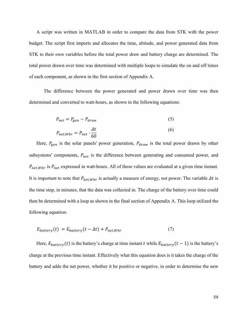
59

A script was written in MATLAB in order to compare the data from STK with the power

budget. The script first imports and allocates the time, altitude, and power generated data from

STK to their own variables before the total power draw and battery charge are determined. The

total power drawn over time was determined with multiple loops to simulate the on and off times

of each component, as shown in the first section of Appendix A.

The difference between the power generated and power drawn over time was then

determined and converted to watt-hours, as shown in the following equations:

𝑃𝑃𝑛𝑛𝑒𝑒𝑛𝑛 = 𝑃𝑃𝑔𝑔𝑒𝑒𝑛𝑛 − 𝑃𝑃𝑑𝑑𝑑𝑑𝑎𝑎𝑑𝑑 (5)

𝑃𝑃𝑛𝑛𝑒𝑒𝑛𝑛,𝑊𝑊ℎ𝑑𝑑 = 𝑃𝑃𝑛𝑛𝑒𝑒𝑛𝑛 ⋅𝛥𝛥𝑡𝑡60

(6)

Here, 𝑃𝑃𝑔𝑔𝑒𝑒𝑛𝑛 is the solar panels' power generation, 𝑃𝑃𝑑𝑑𝑑𝑑𝑎𝑎𝑑𝑑 is the total power drawn by other

subsystems' components, 𝑃𝑃𝑛𝑛𝑒𝑒𝑛𝑛 is the difference between generating and consumed power, and

𝑃𝑃𝑛𝑛𝑒𝑒𝑛𝑛,𝑊𝑊ℎ𝑑𝑑 is 𝑃𝑃𝑛𝑛𝑒𝑒𝑛𝑛 expressed in watt-hours. All of these values are evaluated at a given time instant.

It is important to note that 𝑃𝑃𝑛𝑛𝑒𝑒𝑛𝑛,𝑊𝑊ℎ𝑑𝑑 is actually a measure of energy, not power. The variable 𝛥𝛥𝑡𝑡 is

the time step, in minutes, that the data was collected in. The charge of the battery over time could

then be determined with a loop as shown in the final section of Appendix A. This loop utilized the

following equation:

𝐸𝐸𝑏𝑏𝑎𝑎𝑛𝑛𝑛𝑛𝑒𝑒𝑑𝑑𝑏𝑏(𝑡𝑡) = 𝐸𝐸𝑏𝑏𝑎𝑎𝑛𝑛𝑛𝑛𝑒𝑒𝑑𝑑𝑏𝑏(𝑡𝑡 − 𝛥𝛥𝑡𝑡) + 𝑃𝑃𝑛𝑛𝑒𝑒𝑛𝑛,𝑊𝑊ℎ𝑑𝑑

(7)

Here, 𝐸𝐸𝑏𝑏𝑎𝑎𝑛𝑛𝑛𝑛𝑒𝑒𝑑𝑑𝑏𝑏(𝑡𝑡) is the battery’s charge at time instant 𝑡𝑡 while 𝐸𝐸𝑏𝑏𝑎𝑎𝑛𝑛𝑛𝑛𝑒𝑒𝑑𝑑𝑏𝑏(𝑡𝑡 − 1) is the battery’s

charge at the previous time instant. Effectively what this equation does is it takes the charge of the

battery and adds the net power, whether it be positive or negative, in order to determine the new

60

charge of the battery at the next time instant. A positive net power would indicate that the battery

is being charged, while a negative net power would indicate the battery is losing power.

The battery charge could then be plotted as a function of time. Such graphs show two important

details: first, the recommended DoD, as stated in the battery section of 4.1.2, must not be exceeded,

which can be easily checked upon inspection of the various orbits. Second, if the battery ever

reaches 0Whr, then it is clear that the power profile is unable to accommodate the power budget.

This can be solved either by improving the CubeSat’s pointing in STK, working with other

subsystems to revise the power budget, selecting different hardware, or a combination of these

options.

4.5 Power Subsystem Results

With the methods of selecting hardware and developing a power profile as outlined above, the

team was able to create a subsystem that attempts to meet NeAtO's requirements. Below is an

outline of the final hardware configuration and the results of the final power profile.

4.5.1 Final Hardware Configurations

The hardware used for the CubeSat’s power subsystem was determined early in the design

process. After analyzing the performance capability of each selected component, alternative

components were tested to determine if they met the subsystem requirements more effectively.

Ultimately, however, no hardware was switched out from our initial selection.

The choice for the solar panels was Clyde Space’s Photon-3U body mounted panels (AAC

Clyde Space, 2019). When we were initially designing a 4U CubeSat, these were selected because

Clyde Space no longer provides custom manufactured panels, as they have in years past.

Deployable panels were not considered due to the high drag environment the CubeSat would be

61

exposed to during its mission. When the switch was made to a 6U CubeSat, the 3U panels were

kept, though we did request models of Clyde Space’s Photon-6U panels for the 3U x 2U sides.

These panels would increase the total solar cell area on the satellite's 6U surfaces, thus generating

more power. However, the team had not received such models in time to do a full analysis on them

and thus the Photon-3U was simply attached along NeAtO's eight 3U columns.

The final choice for the EPS was the Starbuck Nano-Plus from Clyde Space (AAC Clyde

Space, 2019). This part was selected as it would be easy to integrate with the other Clyde Space

components. Moreover, it is the only EPS board the company advertises for CubeSats between the

sizes of 3U and 12U. The board itself offers complete control over power distribution and

conversion. It includes MPPT, a PDM, and protection from overcurrent and under-voltage.

The Optimus-40 40Whr battery, again from Clyde Space, was ultimately chosen to store

power. It's operating temperature sits within the range of -10oC and 50oC, which the thermal team

took into account in their analysis (AAC Clyde Space, 2019). Once the swap over to a 6U CubeSat

had been made and the other subsystems had provided their initial power requirements, the power

profiles showed that the charge of the 40Whr battery completely depleted within a matter of days,

thus the Optimus-80 80Whr battery was also considered. However, when running the same profile

models with the Optimus-80, it was found that the 80Whr battery did little more than to extend the

lifetime of NeAtO's’s mission by only a few days, indicating that the battery's storage capabilities

were not the problem as will be discussed in more detail in the following section. Suffice it to say

that once the necessary solution had been found, it was determined that the Optimus-40 battery

was able to handle the new power requirements.

62

4.5.2 Power Profile Results

Determining the orbit that led to optimal power generation consisted of simulating and

comparing different power profiles over various orbits. As we had made our hardware selection

early on in the design process, we were able to simulate these orbits while waiting for the other

subsystems to provide how much power their components drew and when in the orbit they drew

it. With that said, none of the power profiles, including the final profile took into account the initial

maneuver phase or the orbital decay shown in the results of Section 3.5.2 due to the project's time

constraints.

For the final 220-400km orbit, it was found that the panels generated a peak of 17.5W every

orbit, as shown in Figure 21. This is not a constant peak power over the entire mission, however,

as approximately 80 days into the mission there is a gradual dip in power that eventually leads to

a total loss of about 2W in peak power generation, as is illustrated in Figure 22. It was determined

that this drop in power generation is due to the sun vector slowly becoming parallel to the body's

x-z plane. This means that neither of the panels on the 3U x 1U faces were producing their typical

3.5W of power.

Figure 21 - NeAtO early power generation over a single day

63

Figure 22 - NeAtO early power generation over 150 days

A battery charge/discharge was initially determined using the power profile in Figure 22 once

all the other subsystems had provided their components' power states.. It was found that the

selected power hardware would not be able to meet the demands of the other subsystems. The solar

panels did not generate enough power and the battery was completely drained after only nine days.

Switching the battery to the 80Whr battery from Clyde Space extended NeAtO's lifetime to thirteen

days. While deployable solar panels would increase power generation, they were not considered

due to the high drag they would induce. The solution was to revise the power budget. In the end,

the telecommunication subsystem’s power draw was reduced by 1/3 from the original baseline.

The final power budget is displayed in Table 5.

64

Table 5 - NeAtO's final power budget

Group Component How

Many? Peak

Power Nominal Power

Quiescent Power Peak On-Time

Nominal On-Time

Telecomm

Transceiver 1 4 0.48 N/A

Based on coverage times,

⅔ of orbit Never

Antenna 1 2 0.04 N/A

Based on coverage times,

⅔ of orbit Never Payload

NIMS 1 N/A 1.8 N/A N/A

From 240km to

200km Propulsion Engine 4 6 2.5 0.5 Never Never

ADC GPS 1 1.5 N/A N/A Always N/A

OBC 1 1 0.4 N/A Never Always Reaction

Wheels 3 1 N/A N/A Always N/A Gyroscope 1 0.02 N/A N/A Always N/A Fine Sun

Sensors 5 0.01 N/A N/A Always N/A Accelerometer

& Magnetometer 1 0.005 N/A N/A Always N/A

Magnetorquer 3 0.2 N/A N/A Always N/A

With a complete, trimmed power budget, the optimal power profile was found to maintain a

fully charged battery for much of the mission. The Optimus-40 could handle this power draw until

early August, when the solar panels began to produce less power. At that point, the battery slowly

discharged as provided power to other components; in other words, the solar panels could not

generate enough power to charge the battery faster than it discharged. It was initially believed that

65

this loss in battery charge was due to the lesser power being generated by our solar panels in

August. Simulations were rerun within STK using a different pointing orientation for the NeAtO

to test this hypothesis. Instead of being ram-facing and nadir aligned, the satellite was instead set

to keep its ram-facing orientation while being aligned so that a 62° angle was kept between its

body y-axis and the sun vector. This specific angle was selected as it was found to be the angle the

satellite kept until the dip in power generation began the 150 day simulation. The results of our

final simulation, both over a single day and over 150 days, are shown in Figures 23 and 24

respectively.

Figure 23 - Final power generation over a single day

Figure 24 - Final power generation over 150 days

66

Our final power profile was created using the data in Figure 24. The charge of the battery over

a single day early in the mission can be seen in Figure 25. While the battery’s charge fluctuates to

different maximums and minimums with each orbit, it does recharge to 40Whr every couple of

orbits. However, as can be seen from the battery’s charge over the full 150 days in Figure 26,

improving our power generation later in the satellite’s lifetime did not keep the battery from

completely draining. While the battery does not reach 0Whr as early as our previous models, it

does reach it by August 13th.

Figure 25 - Battery charge over a single day

Figure 26 - Battery charge over 150 days

67

While total power generation did lead to the sudden drop off in the battery’s charge, another

logical reason lied in the change in altitude that power is generated over the course of the

spacecraft’s lifetime. Earlier in the spacecraft’s lifetime, peak power generation occurs as NeAtO

approaches perigee in every orbit, as can be seen by the offset of the power wave with the altitude

measurements in Figure 27. However, as time goes on, the solar panels start generating peak power

closer and closer to when the satellite is at apogee. This is best illustrated when looking at the

power generated and the altitude in mid-September, as shown in Figure 28, where the system had

reached its lowest peak power production in previous simulations.

Figure 27 - NeAtO's altitude and power generation over a single day early in the mission

Figure 28 - NeAtO's altitude and power generation over a single day later in its lifetime

Since the times that components require power do not change, this means that as the mission

goes into the later months, more and more power is being taken from the battery and not directly

from what the solar panels are generating. Eventually it reaches the point shown in Figure 28 where

68

the peak power generation occurs at apogee, so the bulk power draw is occurring when there is no

power generation and is thus directly draining the battery. This unfortunately leads to a situation

where the solar panels simply are not capable of recharging the battery as much as it is discharged.

Had the initial detumble and maneuver phases and the orbital decay (Section 3.5.2) been taken

into account, all of the results, from the total generated power to the battery’s lifetime charge,

would have invariably been worse for the mission, though more accurate. Generated power would

vary significantly during detumbling, yet certain components would likely have different power

modes and/or operating times. During the maneuver phase, the generated power would likely be

similar to the current results; however, the thrusters would draw significantly more power and have

different active times as they perform their transfers. As for the orbital decay NeAtO experiences,

it is likely the drop off in power would occur sooner as the components that turn on when

approaching perigee would be in use more frequently.

69

5. Telecommunications Analysis

The telecommunications subsystem provides a means for NeAtO to receive signals and send

data and is comprised of two parts; the hardware on the CubeSat, and the ground stations which

receive data. This chapter describes the entire subsystem in detail, how it was selected, and the

estimated performance.

5.1 Telecommunications Overview

NeAtO's baseline telecommunications system is designed based upon the equipment used in

previous CubeSat projects at WPI. The previous eLEO project, JB-1801 Design and Analysis of

CubeSats in Low Earth Orbit, chose a VHF/UHF Duplex Transceiver and Dipole antenna from

Innovative Solutions In Space (ISISpace). Both instruments operated within the S-Band radio

frequency spectrum.

As for the ground stations, past teams considered a variety of stations, professional and

amateur, including the option of creating a mobile ground station to customize and expand access

points. They also compared various orbital inclinations to find which provided the most access

coverage. It was concluded that an orbit with the same inclination as the ISS (51.6°) was the best

(JB-1801).

Research in the current project focused on finding newer technology and alternative hardware

options, which could improve the subsystem performance and allow for different setups of the

CubeSat.

70

5.1.1 Coverage

The coverage network is extremely important to the success of the telecommunications

subsystem, as such, a reliable and professional network is a high-priority figure of merit when

determining ground stations to communicate with any satellite. The NASA Near-Earth Network

(NASA NEN) is therefore an excellent candidate, due to its extensive history and strategic station

placement, and was used in the previous WPI CubeSat project. Figure 29 shows the stations

comprising the network, and coverage for a 51.6o inclination orbit. The NEN is detailed in the

Nasa Near Earth Network User’s Guide.

Figure 29 - NASA NEN stations with coverage zones (NASA, STK)

In addition to being comprised of all professional or commercial stations, many of them are

located in places with direct sightlines to communicate with the ISS, and have wide fields of view.

Even for heliosynchronous or polar orbits, the network contains multiple stations near the poles.

The network may be well suited to more nominal orbits, but still has enough ground stations to

71

facilitate alternative mission options, with stations that provide better coverage in polar orbits or

other high-inclination orbits (Thoman, Carter, 2016).

5.1.2 Transceiver

The transceiver interfaces with the payload instrument and onboard computer (OBC). It

converts numerical data into signals and relays them to accessible ground stations. These ground

stations in turn send commands to the OBC, which directs the NeAtO and its components. The

strength of the transceiver determines the uplink and downlink capacities, which are the speeds at

which data can be relayed to and received from the satellite by the coverage network. As a

transceiver combines the functions of a radio receiver and a transmitter into one component, it is

not obstructively large. This dual-function component, however, requires more power to run at

maximum data rates, around 20V instead of 10V (IQ-Spacecom). The eLEO CubeSat project (JB-

1801, 2018) utilized the ISIS VHF/UHF Full Duplex Transceiver shown in Figure 30.

Figure 30 - VHF/UHF Duplex Transceiver (ISISpace)

At 0.0096 Mbps and 4W maximum operating conditions, this component is a good candidate

for a CubeSat. It fits easily into an instrument cart, at 90mm x 96mm x 15mm, and with a defined

downlink/uplink schedule, it provides a moderate data rate for a medium power draw.

72

Additionally, it can run only in receiving mode or at low power, down to 0.48W (ISISpace). This

provides the baseline of the NeAtO project.

5.1.3 Antenna

The antenna allows transmission and reception of the physical signals for the CubeSat. There

are a variety of antenna styles, falling into deployable or non-deploying components. Deployable

antennas are lighter and require less power, at the expense of needing extra space to deploy their

fixtures. Non-deployable antennas, also called patch antennas, take up less space and can thus be

mounted in a variety of places. While they do not need to deploy long fixtures, patch antennas

require more power and are heavier. As there is mounting space for deployable antennas in this

project’s CubeSat, the decreased power usage and mass is an attractive feature. Additionally,

deployable antennas for CubeSat missions are readily available and come in various configurations

for different applications, such as monopole for greater signal range and gain, or dipole or turnstile

for greater coverage. The previous projects selected antennas for a balance between antenna gain

and coverage (JB-1801, JB-1701). Such hybrid antennas mitigate the need to point the antenna in

a specific direction. For any antenna type, but especially non-deployable, the placement is very

important, as it will take up space that could otherwise be occupied by solar panels or sensors.

5.2 Hardware Selection

As the goal of the telecommunication subsystem is to provide the fastest possible data transfer

for the CubeSat’s mission, the primary figures of merit are size, speed, and power of the system.

While a fast transfer rate is desired, the system’s efficiency is limited by electric power available

to the spacecraft. Hardware options were compiled from various suppliers, including Clyde Space,

ISIS, Syrlinks, IQ Wireless, and EnduroSat.

73

5.2.1 Transceiver

Transceivers were compared first. Using a combination of separate transmitter and receiver

was immediately disregarded, as having both components would practically double the capacity

the subsystem occupies on an already small spacecraft. Between different transceivers, the

comparison comes down to data speeds and mass. To get the most out of a given coverage pattern,

the data speed should be maximized. The operational frequency capabilities were also compared

consisting of common S-Band equipment which uses 2-4GHz, and newly developed X-Band

equipment of 8-12GHz. X-Band communications operate at the higher frequency and offer much

faster rates. The drawbacks of this equipment are increased mass and power requirements, over S-

Band equipment (Beasly, 2014). Another consideration is Technology Readiness Level (TRL).

While S-Band benefits from being a mature and fully realized technology, X-Band does not. In

comparing equipment in both frequency ranges, there was notably less readily available

information on the X-Band components. Table 6 shows a comparison between both transmitters

and transceivers in S and X band. The bolded columns in both Table 6 and Table 7 indicate that

these were the conditions selected for the mission. Of note are the power requirements and data

rates. While the X-Band equipment looks very promising, most of those components lack detailed

specification sheets, and have not flown on space missions.

74

Table 6 - Transceiver and Transmitter Comparison

Pulsar STX Pulsar XTX

ISIS High Data-rate S-band

ISIS VHF uplink/UHF downlink Full Duplex Transceiver HISPICO X-Band XLink

Company Clyde Space Clyde Space ISIS ISIS IQ Wireless EnduroSat IQ Spacecom

Transmitter Transmitter Transmitter Transceiver Transmitter Transmitter Transceiver

Power <5W <15W 13W .48-4W 4.5-15W 12W 15W

6-12 V 6.2-17V 7-20 V 6.5-20V 3-5V 10-24.5V 7-18V

Mass 100g 130g 120g 75g 75g 270g 200g

Size (mm) 96x90x17.4 96x90x11.7 98.8x93.3x14.5 90x96x15 95x46x15

95.9x90.2x23.6 90x65x28

Temp (oC) -25, +60 -25, +60 -40, +70 -20, +60 -40, +65 -20, +50 Max Rate Down 7.5 Mbps 50 Mbps 4.3 Mbps 0.0096 Mbps 1.06 Mbps 50 Mbps 25 Mbps

Max Rate Up 0.0096 Mbps .064 Mbps

Band S X S S S X X

The ISIS Full Duplex Transceiver was chosen for coverage estimates due to the abundance of

relevant information on it, and that it has been the best choice in previous missions very similar to

this.

5.2.3 Antenna

The selected antenna has to match the transceiver frequency range and not create any

impingement with other components. The impingement concern is particularly important relative

to the solar array, as that affects power generation if the antennas block sunlight from the panels.

As the bus design of NeAtO is subject to change, the manner in which an antenna deploys, and if

75

it deploys, determines if the antenna is compatible. Patch style antennas have to be mounted

externally. This conflicts with the power subsystem, as the external faces of NeAtO are needed for

solar panel mounting. Considering those constraints, the mass and antenna range are the remaining

concerns. Table 7 compares antenna options, both S and X-band.

Table 7 - Transceiver and Transmitter Comparison

ISIS hybrid

X-BAND PATCH ANTENNA SPAN-X-T2 Pulsar SANT

Company ISIS EnduroSat Syrlinks Clyde Space

Power 3.3-5V (Deploy Power) 2W

Size (mm) 98x98x7 24x24x6.4 81.5x89x4.1

Mass 100g 50g

Temp (oC) -20, +60

Notes Deployable Patch Patch Patch

Band S X X S

Range (km) 3000

As the antenna must match the frequency range of the transceiver, an S-Band antenna must be

selected. Regardless, the minimal number of flight-ready X-Band instruments and lack of technical

information on them makes S-Band the frequency of choice. For NeAtO, the antenna is mounted

externally, on the ram-facing (front) side. While the patch antenna is smaller and lighter, the ISIS

Hybrid deploying style was selected. The Pulsar SANT lacked power requirements and antenna

range, which are critical to the estimates conducted to acquire a data budget.

76

5.3 Coverage Estimates

The coverage estimates are central to finding the data budget of the mission. After data rate,

the amount of data that can be sent and received depends on when and for how long access to the

ground stations lasts. Systems ToolKit allows orbits and telecommunications access to be

compared, the Astrogator and telecommunications access features being utilized to create

estimates and detailed schedules of access points. This is significant to the telecom system, as the

position of the CubeSat in coverage regions dictates if uplink/downlink is possible, and the

duration of those accesses dictates the amount of data that can be transferred.

The STK scenario started on a mission start date of May 15th, 2020, at 17:00, with the satellite

orbit being propagated from the parameters in Table 8. A transceiver and antenna were added to

the satellite based on the data from the selected components. The NASA NEN ground stations

were added by latitude and longitude, taking the terrain into account when calculating the view

into space of each site. The coordinates of these sites are listed in Table 9.

Table 8 - STK Scenario Orbit Parameters

Apogee Altitude 440km

Perigee Altitude 200km

Inclination 51.6o

77

Table 9 - Ground Station Coordinates

Station Name Lat (degrees) Long (degrees) Altitude (km)

AGU3 -33.151 -70.666 0.733301

Dongara -29.046 115.349 0.25047

Esrange 67.884 21.061 0.4417

Hartebeesthoek -25.887 27.707 1.568221

McMurdo -77.839 166.667 0.153

North_Pole 64.804 -147.5 0.16058

South_Point 19.014 -155.663 0.367878

Sturup 55.541 13.349 0.1

Svalsat 78.23 15.408 0.501378

Wallops_Island 37.923 -75.477 -0.01064

Weilheim 47.88 11.085 0.663392

White_Sands 32.541 -106.612 1.456545

Figure 31 shows the access periods over 24 hours in the mission. To create estimates of the

data budget, the access from the cube satellite to the ground network was calculated and averaged

over a time period. The total time inside coverage was then multiplied by the transceiver data rate

to give a maximum possible data budget for the period. Once an estimated data coverage per orbit

was found, it could be compared to estimates calculated for different orbits. The access periods in

Figure 31 are represented by a binary state, with high points being times when NeAtO has access

to a ground station, and low points being when it is out of range of the ground stations.

78

Figure 31 - Access periods to ground station network

5.4 Telecommunications Results

The average data budget for one orbit is approximately 11.52Mb, which makes the daily data

budget just about 180Mb with max power. To consider the power constraint, the subsystem runs

at ⅔ full capacity, which means that both power use and data rate will be reduced by a third. This

works in conjunction with the payload on a data schedule so that all data that is generated can be

downlinked in the same orbit period. This meets the subsystem requirements of downklinking as

much data as possible, as fast as possible, without imposing a strain on the power subsystem that

would drastically shorten the mission lifespan.

79

6. Environmental Effects Analysis

Heat physically limits the CubeSat and what it can accomplish in terms of mission longevity

and orbital parameters. If the sun exposure is too much, or the drag induces too much heat, the

CubeSat's physical structure and individual parts within the test bed are at risk of failure. Solar

radiation pressure and ionized oxygen in the plasma environment demand that the CubeSat be

specially coated for protection. This chapter aims to identify the environmental dangers of

spaceflight and to provide explanations on how to protect the satellite during its mission.

6.1 Environmental Effects Overview

Extreme Low Earth Orbits (eLEOs) add more challenges for CubeSats which usually orbit

much higher. Atmospheric winds and drag are present at such low altitudes. If the CubeSat deviates

from its precise course, the mission could fail, as the CubeSat would burn up in the atmosphere.

The previous MQP “Design of CubeSats for Formation Flying & for Extreme Low Earth

Orbit” (NAG-1801, MAD-1801, and JB-1801, 2018) used a number of techniques to prevent

mission failure due to atmospheric interference. With an increased drag force, the MQP team found

that a 4U CubeSat was required over the originally planned 3U design. This was because the

velocity change at the desired altitude of 210km required more fuel for the thrusters. Using an

array of micro pulsed plasma thrusters (μPPTs), the CubeSat could reorient itself at any time to

ensure stability and control during atmospheric interference.

Systems ToolKit (STK) is used to recreate and simulate the environment of the CubeSat’s

orbit. Systems Tool Kit contains many different density models for the atmosphere for any given

orbit. With this simulation, the team can accurately model and graph the atmospheric drag, satellite

temperature, magnetic flux, and power generation from the solar panels throughout each orbit.

80

Previously, MQPs in the past have suggested that atmospheric drag exists and solar winds can add

a level of complexity for each orbit. Using MATLAB, the previous MQPs have calculated

atmospheric drag and fuel consumption for each orbit, but they did not do a full analysis of each

layer of the ionosphere and thermosphere.

6.2 Environmental Effects Research

This team’s mission is to conduct research in the ionosphere with the miniaturized NIMS

payload. The ionosphere ranges from about 50km to almost 1,000km during the most active hours

in the day. The ionosphere gets its name from the fact that UV radiation from the sun activates, or

ionizes, molecular oxygen (O) and nitric oxide (NO). This ionization process requires a lot of

energy and superheats the particles up to 1000K, creating a plasma environment. The spacecraft

will be operating in the F-region of the ionosphere to determine the relationship between the

composition of the ionosphere and weather patterns in this region in order to predict geomagnetic

storms and the impacts thereof upon global communications. The F-region consists of two sub-

regions. The F1 layer is only present during daylight, existing at approximately 150-220km.

Composed of a mixture of O2+, NO+, and atomic O+ ions and with an electron density of 5•105

free electrons/cm3, it merges into the F2 layer at night and drops to roughly 1•104 free

electrons/cm3. The F2 layer is always present at 220-800km during the daytime, composed of

mostly atomic oxygen ions, and will be where this spacecraft spends the majority of its mission.

The nominal electron density is 2•106 free electrons/cm3, but this region is unstable and variations

often occur, especially during magnetic storms.

NeAtO's structural frame harbors all the delicate components that are necessary for the

mission. Chromatic Conversion Coating (CCC) is a chemical process that can help with thermal

properties, electrical contact resistance and corrosion performance. It has been found that using

81

CCCs that have a chromatic solution very close to the very near to the commercial chromating

solution of Alodine 1200S, both the absorptivity and emissivity of the aluminum 7075-T6 can

increase. Allowing for more efficient thermal loading and overall less heat in the structure.

6.3 Modeling Atmospheric Effects

The thermal model for the environmental analysis will be calculated using STK. Required

input parameters include the desired orbit, Earth’s albedo, the material’s absorptivity and

emissivity, dissipated heat from the internal components and spacecraft orientation. The thermal

modeling from STK will provide an estimate of the temperature fluctuations experienced by the

spacecraft throughout a given orbit. Accurate material properties are critical to the accuracy of the

STK thermal model.

STK will also be used to analyze the magnetic flux per orbit in tandem with COMSOL

Multiphysics. STK’s Space Environments and Effects Tool (SEET) package contains a

Geomagnetic Field tool for modeling Earth’s magnetic field. It can provide a visual representation

of magnetic field lines up to 120,000km above Earth, which provides more than enough coverage

for this model. This Geomagnetic Field tool will produce a vector profile of the magnetic flux

through the spacecraft during an orbit, which can then be entered as an input to COMSOL

Multiphysics to analyze the effects of the Earth’s magnetic field as well as any interference due to

the magnetorquers on the spacecraft.

The structures team (NK-2001) selected Aluminium 7075-T6 for the custom 6U CubeSat

frame and provided sources regarding the material properties. Using an Earth albedo of 0.34, a

material absorptivity of 0.9, emissivity of 0.22 and dissipation of 14 watts, this team modeled the

temperature. Figure 32 shows a maximum temperature of 314°C and a minimum of 96°C. This is

82

important because all internal components must function at these temperatures or insulation is

needed to ensure proper function.

Figure 32 - NeAtO External Temperature Versus Solar Intensity

Most of the surface that will be exposed to solar radiation will be solar panels, thus having a

slightly different temperature reading. The solar panels have a high absorptivity of 0.91, but have

a ranging emissivity at each wavelength. While most of the radiation from the sun is in the visible

spectrum, solar panels only emit frequencies in microwaves. This causes high levels of heat to

build up on the surface of the solar panel. Proper ventilation and cooling must be present to ensure

the panels do not overheat.

This team created a simulation for the CubeSat in COMSOL Multiphysics using the same

parameters from STK (see Figure 33). The results showed a maximum temperature of 536K

(263°C) on the ram-facing side. This maximum coincides nicely with the STK average satellite

temperature reading since it falls below that range.

83

Figure 33 - NeAtO's Thermal Profile from COMSOL

While the COMSOL model matches the STK analysis, the results are misleading. The

temperature range is high due to an error in modeling NeAtO. There was a plate added to the RAM

facing side which creates much more drag, absorbs more heat and treats the vehicle as a closed

box with no thermal venting. NeAtO's final design will have the payload replace the plate and two

“holes” that will facilitate ventilation. This is crucial to sustaining a long-term mission and

ensuring thermal stability throughout the internal components.

6.4 Magnetic Interference Modeling

The ADCS team (MAD-2001) chose to use magnetorquers to maintain attitude throughout the

mission. These magnetorquers are functionally solenoids, with a ferrite alloy core wrapped in thin

copper wire. When turned on, these magnetorquers create a magnetic field which acts against the

Earth’s magnetic field, creating a net torque and rotating the spacecraft. This magnetic field is

generated inside the CubeSat, which can potentially cause interference with sensitive instruments

and components of the satellite, such as the onboard computer, the payload, the thrusters, and the

magnetometer, the last of which helps to determine the attitude of the spacecraft by measuring

84

Earth’s magnetic field. This team simulated the magnetic flux throughout the spacecraft in

COMSOL in order to determine if magnetic shielding was necessary.

6.4.1 Modeling a Single Magnetorquer

For a baseline calculation, this team created the model of a single magnetorquer in COMSOL

to analyze its internal magnetic flux and field lines, to guarantee that the model was accurate. The

specifications sheet provided for the magnetorquer provided the magnetic moment, 𝜇𝜇, the radius

of the magnetorquer, the power and voltage required to run the magnetorquer, and the length of

the magnetorquer. The current through the coil, 𝐼𝐼, was calculated using:

𝐼𝐼 = 𝑃𝑃𝑉𝑉

(8)

where 𝑃𝑃 is the power in Watts, and 𝑉𝑉 is the voltage applied. The number of turns, 𝑒𝑒, is calculated

from:

n=𝜇𝜇𝐼𝐼𝐼𝐼

(9)

where 𝐼𝐼 is the current, in amps, and 𝐴𝐴 is the cross-sectional area in square meters, which results in

63,662 turns in the coil on the magnetorquer. These values, and the constants from the specification

sheet, are listed in Table 10.

Table 10 - Constants for determination of turns in magnetorquer coil

Parameter Value

Magnetic moment 0.2Am2

Power 200mW

Voltage 5V

Current 0.04A

85

Radius 0.005m

Cross-sectional area 7.85⋅10-5m2

Length 0.07m

Number of turns in coil 63662

Starting with a single cylinder aligned with the z-axis surrounded by a sphere defined as an

infinite element (i.e. as a vacuum), the Magnetic and Electric Fields (mef) physics engine was

applied within COMSOL. A Coil boundary condition was used on the lateral face of the

magnetorquer to simulate the copper wire, avoiding the need to create a physical model of a coil.

A start condition was specified for the coil, and the COMSOL model produced the models for

magnetic flux density and magnetic field lines as shown below in Figures 34 and 35, respectively.

Figure 34 - Magnetic flux density in single magnetorquer

Figure 35 - Magnetic field lines inside single magnetorquer

The flux distribution internally, as shown in Figure 34, only decreases where the field lines

diverge out of the ends of the magnetorquer due to end effects, remaining even throughout the rest

86

at a value of 0.092T. The field lines as shown in Figure 35 are consistent with expected results and

would produce a magnetic field similar to a bar magnet.

Figure 36 shows the magnetic flux density inside the magnetorquer from its center (0 on the

x-axis of the graph) to one end (0.035m on the x-axis of the graph). The internal magnetic flux

density is constant through the magnetorquer up through 0.025m away from the center, at which

point the end effects take over, which corresponds with the results of the prior two graphs.

Figure 36 - Magnetic Flux Density vs. Distance Along the Z-Axis

6.4.2 Modeling the Earth’s Background Magnetic Field

The next step was to place the defeatured frame of the CubeSat into COMSOL and simulate

the effects of Earth’s magnetic field to guarantee that the frame created negligible magnetic

interference. The SolidWorks CAD file for the frame was exported as an .stp file and imported

directly into COMSOL as its own object as shown in Figure 37. This object required an extremely

87

fine mesh as to account for the intricacies of the frame, which increased processing times for the

physics engine. The CubeSat was placed in a sphere defined with vacuum conditions, and using

the Magnetic Fields, No Currents (MFNC) COMSOL physics engine, a background magnetic field

was defined at 0.04 T, to simulate Earth’s magnetic field at this altitude. Although there is some

interference due to the skeleton of the CubeSat, it amounts to only 0.02nT at most, which is well

below any interference thresholds of the internal instruments, and only occurs localized to the

frame itself.

Figure 37 - Defeatured CubeSat skeleton in COMSOL

88

7. Thermal Vacuum Chamber Preliminary Research

This MQP is responsible for the preliminary design of a Thermal Vacuum Chamber (TVaC)

with which to subject the structural and electrical of the spacecraft to thermal loading relevant to

what it would experience during the mission profile. While the scope of this project is not to build

and implement the TVC, the following section aims to lay the groundwork for future WPI CubeSat

projects to use as reference in their own TVC design.

7.1 Testing Applications and Standards

Spacecraft experience extreme pressures and temperatures not found on Earth. Thermal

Vacuum Chambers provide the means of testing the reliability and functionality of a spacecraft

hardware under thermal cycling and low pressures. While similar analysis can be done in programs

such as COMSOL and ANSYS, a TVC provides a means to physically demonstrate the

environment and verify and validate simulations.

Tests are often done in compliance with standards established by the US Military. Relevant to

this mission are the procedures defined in MIL-STD-202 and NASA-STD-7002b. The MIL-STD-

202 describes methods with which to test the effects of isolated variables on electronic and

electrical components while the NASA-STD-7002b describes methods to test the structural

integrity of various materials within an accepted safety factor (NASA, 2018). The procedures

presented in these documents are to be taken as guidelines; conducting the tests requires tailoring

the methods as the situation requires.

With respect to MIL-STD-202, the vacuum chamber can comply with test methods 105C

(Barometric Pressure) and 107G (Thermal Shock). 105G outlines the dangers high altitude flight

can have on electric components. Low pressures may subject the components to dielectric-

89

withstanding-voltage failure, weaker electrical contacts, and high pressure differentials along

seals. The air's increased thermal insulation mitigates heat transfer, thus internally generated heat

will remain near its source. As a result of these effects, the dielectric constant (a measure electric

insulation) of the component decreases (Department of Defense, 2002).

The Thermal Shock tests described in section 107G of the MIL-STD-202 can be used to

explore the effects of extreme temperature cycling the CubeSat will undergo throughout its orbit.

The application and distribution of heat on components over thermal cycles causes non-uniform

deformation of various portions of the component. These deformations can lead to cracks, fillings

leakage, weakened seals, and mechanical displacement of electrical materials (Department of

Defense, 2002).

The NASA-STD-7002b document provides design and test requirements materials must

adhere to in order to be flight-worthy, as decided by NASA administration. It specifies duration

and safety factors for environmental testing, expected results from functional demonstrations, and

margins of acceptable performance.

90

8. Conclusions, Recommendations, and Social Impacts

This chapter provides recommendations that will assist in future CubeSat projects and reveal

effective solutions to the problems encountered in the design and analysis process by the various

subsystems of NeATo. The chapter concludes with the educational impacts of the CubeSat

technology.

8.1 Payload Summary

The INMS payload carried onboard the 6U NeATo maintained a duty cycle of 8.9% for the

mission, turning on at 240 km altitude and off at 200 km altitude. This duty cycle produces 6.61

Mb of data per orbit, or 10.58 Mb data per day, which will be downloaded for analysis via the

Ground Station Network. Collection profiles were planned for activation altitudes between perigee

and 300 km. The 240-200 km duty cycle was selected in order to collect meaningful scientific data

at the F1/F2 transition boundary in the ionosphere, while minimizing the power draw for various

subsystems, ultimately achieving the design goal.

8.2 Propulsion and Orbital Analysis

Orbit analysis was performed using the STK software. The propulsion subsystem is based on

the Busek BET-300P electrospray thruster. It is able perform an orbit transfer from the deployment

from the ISS at an altitude of 400 km to an elliptical orbit with an apogee of 440 km and a perigee

of 200 km. This orbit transfer requires approximately 35.2g of propellant. Once NeATo reaches

the desired orbit, the propulsion subsystem allows it to stay in orbit for 45 days, using the

remaining 28g of propellant. For comparison without propulsion our analysis shows that the

NeATo would deorbit in 16 days.

91

8.3 Power Analysis

The power subsystem consists of Clyde Space’s Photon-3U body mounted solar panels,

Starbuck Nano-Plus EPS board, and Optimus-40 40Whr battery. The subsystem is capable of

providing a consistent 17.5W for approximately 80 days from the beginning of the mission. This

power is adequate to operate the rest of the subsystems at a reduced power. After 80 days, the

battery is expected to completely drain and become unable to recover. The power subsystem can

remain operational for twice as long the propulsion subsystem can, this does not mean the power

budget for those first 45 day would change. As the telecommunications operation was deemed to

have less of an effect on the success of the scientific mission than the ADCS and payload operation,

it was the first subsystem to have its power budget reduced for the sake of prolonging the mission

time.

8.4 Telecommunications Analysis

The telecommunication subsystem has an 180 Mb of daily downlink and uplink capacity. The

subsystem can sustain this daily data rate for the entire mission on reduced power, for as long as

the orbit and power level can be sustained. The reduced data option of the payload, and reduced

power level of the telecom instruments do limit the mission productivity, but allow for a much

longer lifespan than would be possible otherwise. This allows more data to be taken for a long

period of time, which may produce more useful results.

8.5 Environmental Effects Analysis

Given the maximum temperature in sunlight, the metal frame of NeAtO will survive, but the

solar panels could be at risk due to high absorptivity and high drag. Thermal shock also adds a

level of complexity as the internal stress on each component and soldered wire can lead to

92

electronic failure. In order to fully understand the impact of thermal shock on NeAto, an

experiment should be conducted in a thermal vacuum chamber. The environment produced can

simulate the space environment and can show whether or not thermal shock will cause component

failure. Meanwhile, the magnetorquers produce a magnetic flux density of 0.092 T, four orders of

magnitude higher than Earth’s background magnetic field. As a result, if the magnetic flux at a

single component exceeds the component’s own shielding, future projects will need to consider

external shielding for mission survival.

8.6 Recommendations

The following section provides recommendations to be considered for future iterations on the

NeATo CubeSat. They reflect the shortcomings of each subsystems' analysis and offer ideas for

what will improve the process and results of those future missions.

1. General Project Management

● Define and share a master simulation file for all subsystem teams to utilize and modify as

needed. This will keep teams from wasting time recreating simulations that have already

been used elsewhere.

2. Payload

● Consider an inactive “survival period” where no data is collected for a number of orbits to

allow for the battery to recharge in order to extend mission lifespan.

3. Propulsion

● Consider the use of propellant tanks to increase the amount of propellant available for the

thruster. This will help increase the mission lifespan.

93

4. Power

● Take orbital decay into consideration. As the orbit decays, components which activate at

lower altitudes draw power for larger portions of the orbit. A profile that addresses this

issue will be more accurate.

● Select solar panels that cover the maximum surface area.

● Use the equation for solar panels' power generation to optimize the angle of incidence

throughout the mission.

5. Telecommunications

● Be persistent and obtain full component specifications from suppliers.

● Make use of available X-Band equipment.

● Take orbital decay into consideration and address how it affects coverage windows.

● Look into the possibility of using multiple antenna and transceiver pairings to increase data

rate.

6. Environmental Effects

● Perform a full 3-D COMSOL simulation of the CubeSat, with all three magnetorquers

active, in order to determine magnetic flux upon each sensitive component.

● Perform magnetic impact analysis for various orbits considering variations in the Earth’s

magnetic field.

● Consider the impacts of radioactive environments on the CubeSat, and guarantee essential

components are radiation hardened if this is deemed an issue.

94

8.7 Social Impacts of CubeSats

CubeSats provide unique opportunities for students to gain hands-on experience through which

they can exercise the skills and knowledge they have gained in a traditional lecture setting. More

and more higher education STEM institutions are turning to project-based learning (PBL) to give

their students a real-world understanding of the material. Studies have shown that PBL can lead to

higher average examination scores; Freeman et al. (2015) claim that exam scores were increased

by 6% in classes with active learning projects and that students in courses with solely traditional

lecturing are 1.5 times more likely to fail out of that class (S. Freeman, S.L. Eddy, M. McDonough,

M.K. Smith, N. Okoroafor, H. Jordt, and M.P. Wenderoth, 2014).

Not only is PBL a more effective method of teaching difficult material, it also places the

students in a position they may never have been in before. CubeSats are specifically effective at

exposing students to the complicated process of designing a multi-subsystem project. The design

and functionality of any one subsystem is strongly linked to the design and function of the others.

Creating a functioning CubeSat requires effective communication between project members and

that each member has an understanding of the system as a whole. Compared to scientific missions

that require large, complex spacecraft, CubeSat projects offer more leeway for success in several

aspects of design that lends itself directly to an effective educational experience: missions often

consist of simple orbital maneuvers and passive data collection; the satellite consists of few

subsystems, all dedicated to completing the primary mission; the small frame and standardized

sizing invoke a short construction timeline; and ambiguous or loosely defined mission

characteristics encourage creative thinking (National Academies of Sciences, Engineering, and

Medicine, 2016).

95

The educational benefits of a large CubeSat program can be seen on the campus of the

University of North Dakota, where the OpenOrbiter Small Spacecraft Development Initiative

(OOSSDI) launched in 2012. The program aims to demonstrate the opportunities in 1U

NanoSatellites, which can be designed and constructed from off-the-shelf hardware for under

$5,000. While it is easy to say that project-based programs like this help to give the students real-

world experience, it is difficult to quantify just how much it actually affects the students' academic

capabilities. According to Straub et al. (2013), there is a correlation between duration of

participation in the program and various indicators of academic ability. The study surveyed

students associated with OOSSDI and compared their self-reported improvement (not overall

competency) in areas such as Technical Skill, Spacecraft Design, and Space Excitement with

variables including years in the program, hours spent per week on the project, overall GPA,

undergraduate/graduate status, and more (Straub & Whalen, 2014).

The main conclusions were that hours spent per week on OOSSDI, years participating in

the program, and having the role as team lead all had a strong correlation with overall academic

improvement. There was no significant correlation between GPA, undergraduate versus graduate

students, and class level with aggregate growth. The variables which related to the students to their

role and responsibility within OOSSDI all correlated with improvement while the variables

defined independently of the students' connection to OOSSDI showed no correlation with

improvement. Given these results, the study concluded that the NanoSat program had a positive

influence on its students (Straub & Whalen, 2014).

At WPI over the past five years, three MQPs have been conducted on various Cubesat

missions. Unlike large spacecraft, the availability of COTS components for Cubesats allowed the

96

students of these projects to proceed with a complete spacecraft design. The MQPs provided a

realistic and unique exercise in spacecraft and mission design.

97

Works Cited

AAC Clyde Space. Solar Panels - Photon (2019, August 1). PDF. Retrieved from

https://www.aac-

clyde.space/assets/000/000/078/PHOTON_original.pdf?1564954830

AAC Clyde Space. Battery - Optimus (2019, August 1). PDF. Retrieved from https://www.aac-

clyde.space/assets/000/000/079/OPTIMUS_original.pdf?1564954960

AAC Clyde Space. Power Distribution and Conditioning Units - Starbuck-Nano (2019, August

1). PDF. Retrieved from https://www.aac-clyde.space/assets/000/000/103/STARBUCK-

NANO_original.pdf?1565681302

Agasid, E., Burton, R., Carlion, R., Defouw, G., Perez, A. D., Karacalioglu, A. G., … Weston, S.

(2018, December). PDF. Moffett Field.

AGI . (2019, December). COLLADA Models. Retrieved from

http://help.agi.com/stk/index.htm#vo/modelImport.htm.

AGI. Blender Modelling and Articulations for STK Users. (n.d). PDF.

Beasley, J., & Miller, G. M. (2014). Modern electronic communication. Harlow: Pearson.

Blandino, J.J., Martinez, N., Demetriou, M. A., Gatsonis, N. A., Paschalidis, N., “Feasibility for

Orbital Life Extension of a CubeSat Flying in the Lower Thermosphere”, Journal of

Spacecraft and Rockets, Vol. 53, No. 5, pp. 864-875, 2016. DOI:10.2514/1.A33462

98

Clark, C., & Simon, E. (2007). Evaluation of Lithium Polymer Technology for Small Satellite

Applications. Retrieved December 17, 2019, from

https://digitalcommons.usu.edu/smallsat/2007/all2007/66/

Courtney, Daniel G., et al. “Electrospray Thrusters for Small Spacecraft Control: Pulsed and

Steady State Operation.” 2018 Joint Propulsion Conference, 2018, doi:10.2514/6.2018-

4654.

Curci, E. A., Jacobson, J. B., Slabinski, K. M., & Schlack, W. T. (2017). Design and Analysis for

the Sphinx-NG CubeSat. Retrieved from https://digitalcommons.wpi.edu/mqp-all/3638

Department of Defense. Test Method Standard: Electric and Electronic Component Parts (2002).

Columbus, OH.

Dunbar, Brian. “Ion Propulsion.” NASA, NASA, 18 Aug. 2015, Retrieved from

www.nasa.gov/centers/glenn/about/fs21grc.html.

Electrospray Thrusters Boost Efficiency, Precision. NASA, NASA, Retrieved from

spinoff.nasa.gov/Spinoff2016/ip_9.html.

Freeman, S., Eddy, S.L., McDonough, M., Smith, M.K., Okoroafor, N., Jordt, H., and

Wenderoth, M.P. (2014). Active learning increases student performance in science,

engineering, and mathematics, Proceedings of the National Academy of Sciences

111(23):8410-8415.

Garner, R. (2018, October 22). Dellingr: The Little CubeSat That Could. Retrieved from

https://www.nasa.gov/feature/goddard/2018/dellingr-the-little-cubesat-that-could

99

Gatsonis, N.A., Ye, L., Blandino, J.J., Demetriou, M., Paschalidis, N., “Micro Pulsed Plasma

Thrusters for Attitude Control of a Low Earth Orbiting CubeSat,” Journal of Spacecraft

and Rockets, Vol. 53, No. 1, pp. 57-73, 2016. DOI: 10.2514/1.A33345.

Hall, Nancy. “Solid Rocket Engine.” NASA, NASA, Retrieved from

www.grc.nasa.gov/WWW/K-12/airplane/srockth.html.

Henry, C. (2019, September 7). SpaceX says more Starlink orbits will speed service, reduce

launch needs. Retrieved from https://spacenews.com/spacex-says-more-starlink-orbits-

will-speed-service-reduce-launch-needs/

Horvath, G., Marosy, G., Glisics, S., & Czifra, D. (2012). Battery characterization for CubeSat

missions with battery tester application. 2012 13th Biennial Baltic Electronics

Conference. doi: 10.1109/bec.2012.6376824

Jeffrey, Davidson, Ryan, Earle, Greg, Halford, … Rob. (2018, July). PetitSat - a 6U CubeSat to

examine the link between MSTIDs and ionospheric plasma density enhancements.

Retrieved from https://ui.adsabs.harvard.edu/abs/2018cosp...42E1773K/abstract

Jenner, L. (2017, May 9). NASA Team Pursues Blobs and Bubbles with New PetitSat Mission.

Retrieved from https://www.nasa.gov/feature/goddard/2017/nasa-team-pursues-blobs-

and-bubbles-with-new-petitsat-mission

Jenner, L. (2017, August 2). NASA Set to Launch Dellingr. Retrieved from

https://www.nasa.gov/feature/goddard/2017/nasa-set-to-launch-dellingr-cubesat-

purposely-designed-to-improve-reliability-of-small-0

JPL: NASA. (n.d.). Missions. Retrieved from https://www.jpl.nasa.gov/cubesat/missions/

100

K., S. (2009, January 1). THERMOPHYSICAL AND ELECTRICAL PROPERTIES OF

CHROMATE CONVERSION COATINGS ON ALCLAD AA7075-T6 ALUMINUM

ALLOY. Retrieved from https://www.sid.ir/en/Journal/ViewPaper.aspx?ID=175658

Kalde, J. (2012, July). System architecture of the ESTCube-1 satellite power system. Retrieved

from http://jaanus.tech-thing.org/space/more-details-electrical-power-system/

Kant, A. B., Nichols, J. J., Mancinelli, L. J., Knodler, M. J., Abad, M. F., Escalante-Hurtado, M.,

& Crockett, R. C. (2018). Design and Analysis of CubeSats in Low Earth Orbit.

Retrieved from https://digitalcommons.wpi.edu/mqp-all/3885

Kewen Z., Gatsonis, N.A., Blandino, J. J., Demetriou, M. A., “Nanosat Orbit Raising and

Rendezvous Using a Continuous-Thrust Controller,” AIAA 2017-0163, 55th AIAA

Aerospace Sciences Meeting, Grapevine TX, Jan. 9-13, 2017.

Loff, S. (2015, July 22). CubeSats Overview. Retrieved from

https://www.nasa.gov/mission_pages/cubesats/overview.

Markets and Markets. (n.d.). CubeSat Market. Retrieved from

https://www.marketsandmarkets.com/Market-Reports/cubesat-market-

58068326.html?gclid=Cjw

Missions Launched. Retrieved from http://www.polysat.org/launched

Monopropellant Rocket Engines. Monopropellant Rocket Engines | Aerojet Rocketdyne,

www.rocket.com/space/space-power-propulsion/monopropellant-rocket-engines.

101

Moorthy, A.K., J. J. Blandino, M. A. Demetriou, N. A. Gatsonis, "Extended Orbital Flight of a

CubeSat in the Lower Thermosphere with Active Attitude Control", AIAA 2019-1518,

AIAA Scitech 2019 Forum, January 2019. DOI: 10.2514/6.2019-1518.

Moorthy, A.K., J. J. Blandino, M. A. Demetriou, N. A. Gatsonis, “Orbit Maintenance and

Attitude Control for a CubeSat Flying in the Lower Thermosphere”, AIAA 2018-5404,

AIAA Space 2018, September, 2018. DOI: 10.2514/6.2018-5404.

NASA. State of the Art Small Spacecraft Technology. (2018, December). PDF. Retrieved from

https://www.nasa.gov/sites/default/files/atoms/files/soa2018_final_doc.pdf

National Academies of Sciences, Engineering, and Medicine. 2016. Achieving Science with

CubeSats: Thinking Inside the Box. Washington, DC: The National Academies Press.

doi:10.17226/23503

Navarathinam, N., Lee, R., & Chesser, H. (2011). Characterization of Lithium-Polymer batteries

for CubeSat applications. Acta Astronautica, 68(11-12), 1752–1760. doi:

10.1016/j.actaastro.2011.02.004

NSF. Award Search: Award#1719200 - Collaborative Research: RAPID: Exocube 2 - A Cubesat

to Measure In-situ the Global Distribution of Light Species Densities in the Exosphere.

Retrieved from https://www.nsf.gov/awardsearch/showAward?AWD_ID=1719200

NSF. National Science Foundation Annual Report (2013). PDF. Wallops Island. Retrieved from

https://www.nsf.gov/geo/ags/uars/cubesat/nsf-nasa-annual-report-cubesat-2013.pdf

Pultarova, T. (2017, April 19). Could Cubesats Trigger a Space Junk Apocalypse? Retrieved

from https://www.space.com/36506-cubesats-space-junk-apocalypse.html.

102

Rodriguez, M., Paschalidis, N., Jones, S., Sittler, E., Chornay, D., & Uribe, P. Miniaturized Ion

and Neutral Mass Spectrometer for CubeSat Atmospheric Measurements. (2016, August

6). PDF. Retrieved from:

https://ntrs.nasa.gov/archive/nasa/casi.ntrs.nasa.gov/20160010304.pdf

Spectrolab. (2018, July 16). PDF. Sylmar, California.

Straub, J., & Whalen, D. (2014). Evaluation of the Educational Impact of Participation Time in a

Small Spacecraft Development Program. Education Sciences, 4(1), 141–154. MDPI AG.

Retrieved from http://dx.doi.org/10.3390/educsci4010141

Thoman, B. E., & Carter, D. L. (2016, February 24). Near Earth Network (NEN) Users’ Guide.

Retrieved from https://sbir.gsfc.nasa.gov/sites/default/files/453-NENUG R2.pdf

Wall, M. (2019, April 24). Meet OSCaR: Tiny Cubesat Would Clean Up Space Junk. Retrieved

from https://www.space.com/space-junk-cleanup-cubesat-oscar.html.

Wertz, J. R., & Larson, W. J. (1999). Space mission analysis and design (3rd ed.). Torrance, CA:

Microcosm.

103

Appendices

Appendix A: Battery Charge Code

104

105

106

107

108

Appendix B: Sample STK Data for Battery Charge

Time (UTCG) Power (W) Altitude (km)

5/15/2020 17:13 0 300.765076

5/15/2020 17:14 0 292.308806

5/15/2020 17:15 0 283.930238

5/15/2020 17:16 0 275.678954

5/15/2020 17:17 0 267.605695

5/15/2020 17:18 7.526 259.761928

5/15/2020 17:19 7.687 252.199365

5/15/2020 17:20 7.25 244.969447

5/15/2020 17:21 6.975 238.122792

5/15/2020 17:22 6.845 231.708628

5/15/2020 17:23 6.921 225.774203

5/15/2020 17:24 7.206 220.364205

5/15/2020 17:25 7.604 215.520179

5/15/2020 17:26 8.147 211.279974

5/15/2020 17:27 8.783 207.677224

5/15/2020 17:28 9.49 204.740865

109

5/15/2020 17:29 10.236 202.494725

5/15/2020 17:30 10.996 200.957168

5/15/2020 17:31 11.749 200.14082

5/15/2020 17:32 12.502 200.052385

5/15/2020 17:33 13.218 200.692536

5/15/2020 17:34 13.906 202.055912

5/15/2020 17:35 14.548 204.131195

5/15/2020 17:36 15.134 206.901286

5/15/2020 17:37 15.682 210.343561

5/15/2020 17:38 16.16 214.430204

5/15/2020 17:39 16.581 219.128615

5/15/2020 17:40 16.923 224.401872

5/15/2020 17:41 17.216 230.209246

5/15/2020 17:42 17.418 236.50675

5/15/2020 17:43 17.567 243.247711

5/15/2020 17:44 17.631 250.383358

5/15/2020 17:45 17.622 257.863404

5/15/2020 17:46 17.552 265.636623

110

5/15/2020 17:47 17.407 273.651403

5/15/2020 17:48 17.198 281.85627

5/15/2020 17:49 16.903 290.200375

5/15/2020 17:50 16.554 298.63394

5/15/2020 17:51 16.143 307.108653

5/15/2020 17:52 15.658 315.578016

5/15/2020 17:53 15.125 323.997636

5/15/2020 17:54 14.542 332.325472

5/15/2020 17:55 13.911 340.522015

5/15/2020 17:56 13.236 348.550432

5/15/2020 17:57 12.54 356.376653

5/15/2020 17:58 11.805 363.96941

5/15/2020 17:59 11.08 371.300239

5/15/2020 18:00 10.318 378.343443

5/15/2020 18:01 9.598 385.076016

5/15/2020 18:02 8.903 391.477543

5/15/2020 18:03 8.261 397.530069

5/15/2020 18:04 7.703 403.217956

111

5/15/2020 18:05 7.274 408.527713

5/15/2020 18:06 6.982 413.447822

5/15/2020 18:07 6.847 417.96856

5/15/2020 18:08 6.892 422.081808

5/15/2020 18:09 7.112 425.780869

5/15/2020 18:10 7.495 429.060294

5/15/2020 18:11 7.999 431.915706

5/15/2020 18:12 8.582 434.343644

5/15/2020 18:13 0.285 436.341425

5/15/2020 18:14 0 437.90701

5/15/2020 18:15 0 439.038906

5/15/2020 18:16 0 439.736076