Design, Analysis, Assembly, Integration and Testing of Mechanical … · 2015-04-24 · Design,...
126
Design, Analysis, Assembly, Integration and Testing of Mechanical Systems for Micro-Satellites and Micro-Satellite Separation Systems by Jamie Fine A thesis submitted in conformity with the requirements for the degree of Master of Applied Science Graduate Department of Aerospace Science and Engineering University of Toronto © Copyright by Jamie Fine 2014
Transcript of Design, Analysis, Assembly, Integration and Testing of Mechanical … · 2015-04-24 · Design,...

Design, Analysis, Assembly, Integration and Testing of Mechanical Systems for Micro-Satellites and
Micro-Satellite Separation Systems
by
Jamie Fine
A thesis submitted in conformity with the requirements for the degree of Master of Applied Science
Graduate Department of Aerospace Science and Engineering University of Toronto
© Copyright by Jamie Fine 2014

Design, Analysis, Assembly, Integration and Testing
of Mechanical Systems for Micro-Satellites and
Micro-Satellite Separation Systems
Jamie Fine
Master of Applied Science
Graduate Department of Aerospace Science and Engineering
University of Toronto
2014
Abstract
This document summarizes the development activities completed for the Exoadaptable Pyroless
Deployer (XPOD) system, and the MiniMags, EV9 and NORSAT-1 missions. The focus is on
the mechanical design, computer modelling, and assembly integration and testing of mechanical
systems. The XPOD work was associated with a re-analysis and testing of the XPOD Triple
engineering model such that a flight model could be produced. The MiniMags work involved
creating a preliminary bus design, which was ultimately used to determine that the MiniMags
payload could feasibly be flown in a microsatellite. The EV9 work included taking the EV9 bus
design from a mature design stage to flight assembly. Finally, work for the NORSAT-1 mission,
which is a microsatellite mission with several different payloads, took a proposal level bus
mechanical design to a preliminary design such that future work could be continued in later
stages of the mission.

Acknowledgments
The last two years would not have been possible without the help of so many people. Whether
the help was through a casual guiding conversation, moral support and encouragement, daily
management, or finances, it was all needed to work through the challenges that were
encountered.
I would like to thank Dr. Robert Zee for the opportunity that he provided me with by allowing
me to complete my degree at the Space Flight Laboratory. Nathan, for keeping me busy and
providing me with direction in my work, along with all the epic Frisbee games at lunch. Freddy,
for all of his guidance with the XPOD system. Mike for not only his help with the XPODs, but
also for his teachings on how to get ideas from a computer onto a lab bench. Laura, for helping
me learn how to integrate a flight spacecraft. Brad (“The Smurds”... haha), Tom, Josh and John
for all of their moral support, helpful conversations, and great/hilarious times in and out of the
lab.
To my parents I would like to thank you for supporting me through my second degree. To
Kseniya, thank you for always helping me with getting through the tough days no matter how
busy or tired we both were.
Finally, I would like to thank everyone else who made the hard days a little less difficult, the
tiring days a little less tiring, and the good days a little better. I learned so much in the past two
years about not only engineering, but about who I am, and about what is important to me in my
life.

Table of Contents
Acknowledgments .......................................................................................................................... iii
Table of Contents ........................................................................................................................... iv
List of Tables ................................................................................................................................ vii
List of Acronyms ......................................................................................................................... viii
List of Figures ................................................................................................................................ ix
Introduction .................................................................................................................... 1
1.1 The Exoadaptable Pyroless Deployer ................................................................................. 1
1.1.1 Separation Systems Overview ................................................................................ 1
1.1.2 Exoadaptable Pyroless Deployer Operation Method .............................................. 3
1.2 The MiniMags Feasibility Study ........................................................................................ 7
1.3 The EV9 Mission ................................................................................................................ 9
1.4 The NORSAT-1 Mission .................................................................................................. 10
1.5 Thesis Objectives .............................................................................................................. 12
Mechanical Systems Design ......................................................................................... 14
2.1 Derivation of Mechanical Requirements .......................................................................... 14
2.2 XPOD Mechanical Design ................................................................................................ 17
2.2.1 Mechanical Design of the XPOD Mechanism, Internal Preload and Main
Spring .................................................................................................................... 17
2.2.2 XPOD Mechanism Overview ............................................................................... 17
2.2.3 Pusher Plate Preload Design ................................................................................. 19
2.2.4 Designing the Main Spring ................................................................................... 26
2.2.5 Determining the Required Tension in the Mechanism Cord ................................ 31
2.2.6 Determining the Mechanism Jamming Conditions ............................................... 36

2.3 XPOD Tip Off Rate Analysis ........................................................................................... 38
2.3.1 Problem Definition ................................................................................................ 38
2.3.2 Assumed Ejection Geometry for Limiting Angles ............................................... 39
2.3.3 Relevant Equations ............................................................................................... 50
2.3.4 Implementation of the Solution Method ............................................................... 58
2.3.5 Tip-Off Rate Analysis Results .............................................................................. 63
2.4 EV9 Mechanical Design ................................................................................................... 65
2.4.1 EV9-A vs. EV9 vs AISSat-2 Comparison ............................................................ 65
2.4.2 EV9 Mechanical Design Requirements ................................................................ 66
2.4.3 Design Process ...................................................................................................... 67
2.5 NORSAT-1 Mechanical Design ....................................................................................... 79
2.5.1 NORSAT-1 Design Requirements and Starting Point .......................................... 79
2.5.2 NORSAT-1 Design Iterations ............................................................................... 81
Finite Element Modelling ............................................................................................. 89
3.1 MiniMags Finite Element Model ...................................................................................... 89
3.2 Finite Element Model Setup ............................................................................................. 90
3.2.1 Boundary Conditions ............................................................................................ 90
3.2.2 Modelling Methodology ....................................................................................... 91
3.2.3 Material Selection ................................................................................................. 92
3.3 Results ............................................................................................................................... 92
3.3.1 Natural Frequencies .............................................................................................. 93
3.3.2 Stress Results ........................................................................................................ 94
3.4 Conclusions ....................................................................................................................... 97
Assembly Integration and Testing ................................................................................ 98
4.1 XPOD Triple Vibration Testing ........................................................................................ 98
4.1.1 Axis Definition and Mounting Location ............................................................... 98

4.1.2 Accelerometer Placement ..................................................................................... 99
4.1.3 Vibration Levels .................................................................................................. 101
4.1.4 Inspection Procedure ........................................................................................... 102
4.1.5 Vibration Test Procedures ................................................................................... 108
4.2 EV9 Horizontal Deployment Test .................................................................................. 109
4.2.1 Spring Constant Determination Procedure ......................................................... 110
4.2.2 Deployment Test Procedure ................................................................................ 111
Conclusion .................................................................................................................. 114
References ................................................................................................................................... 116

List of Tables
Table 1: Overview of Qualified XPOD Designs ............................................................................ 1 Table 2: Launch Vehicle Mechanical Environment Summary ..................................................... 14
Table 3: List of Input Variables Used in Calculations and MATLAB Code ................................ 49 Table 4: Summary of Tip-Off Rate Analysis Verification ........................................................... 64 Table 5: Bus Subsystems Summary .............................................................................................. 65 Table 6: List of NORSAT-1 Relevant Mechanical Requirements ............................................... 81 Table 7: Summary of Material Properties Used in the MiniMags FEM ....................................... 92
Table 8 - List of Accelerometers ................................................................................................ 100
Table 9: List of Images ............................................................................................................... 104 Table 10: List of Measurements ................................................................................................. 107

List of Acronyms
SFL Space Flight Laboratory
XPOD eXoadaptable PyrOless Deployer
GNB Generic Nanosatellite Bus
RAL Rutherford Appleton Laboratory
CSA Canadian Space Agency
PCW Polar Communications and Weather
HEO Highly Elliptical Orbit
MiniMags Mini-Magnetosphere Shield
LV Launch Vehicle
FEM Finite Element Model

List of Figures
Figure 1.1-1: Images of Currently Qualified XPODs ..................................................................... 2 Figure 1.1-2: XPOD with Labelled Internal Components .............................................................. 3
Figure 1.1-3: XPOD External Components with Labels ................................................................ 4 Figure 1.1-4: Parts of the XPOD Mechanism with Labels ............................................................. 5 Figure 1.1-5: XPOD Arming Steps ................................................................................................. 6 Figure 1.2-1: Van Allen Belt Illustration [4] .................................................................................. 8 Figure 1.4-1: NORSAT-1 PDR Stage Bus Design Overview ...................................................... 11
Figure 2.2-1: Isometric View of XPOD Triple Mechanism before Deployment ......................... 18
Figure 2.2-2: Simplified XPOD Mechanism Actuation Sequence ............................................... 18 Figure 2.2-3: Section View of XPOD Pusher Plate with Labels .................................................. 20
Figure 2.2-4: XPOD GNB Bellville Stack .................................................................................... 21 Figure 2.2-5: Exploded View of XPOD GNB Stack .................................................................... 22 Figure 2.2-6: Bellville Washer Diagram with Labels [14] ........................................................... 22 Figure 2.2-7: Bellville Stacking Arrangement Example ............................................................... 24
Figure 2.2-8: Simplified View of a XPOD GNB Door ................................................................ 31 Figure 2.2-9: Door Free Body Diagram ........................................................................................ 31
Figure 2.2-10: FBD of Mechanism without Internal Forces ......................................................... 33 Figure 2.2-11: FBD of Mechanism with Internal Forces .............................................................. 34
Figure 2.2-12: FBD of XPOD Door ............................................................................................. 35 Figure 2.2-13: FBD of Left Clamp ............................................................................................... 35
Figure 2.3-1: Geometry Overview for Tip-Off Rate Analysis ..................................................... 39 Figure 2.3-2: Geometry Overview for Tip-Off Rate Analysis after Pusher Plate Separation ..... 40 Figure 2.3-3: Stage One Ejection Geometry Overall View .......................................................... 41
Figure 2.3-4: Stage 1 Ejection Zoom 1 ......................................................................................... 41 Figure 2.3-5: Stage 1 Ejection Zoom 2 ......................................................................................... 41
Figure 2.3-6: Stage Two Ejection Geometry Overall View ......................................................... 42 Figure 2.3-7: Stage 2 Ejection Zoom 1 ......................................................................................... 42 Figure 2.3-8: Stage 2 Ejection Zoom 2 ......................................................................................... 43
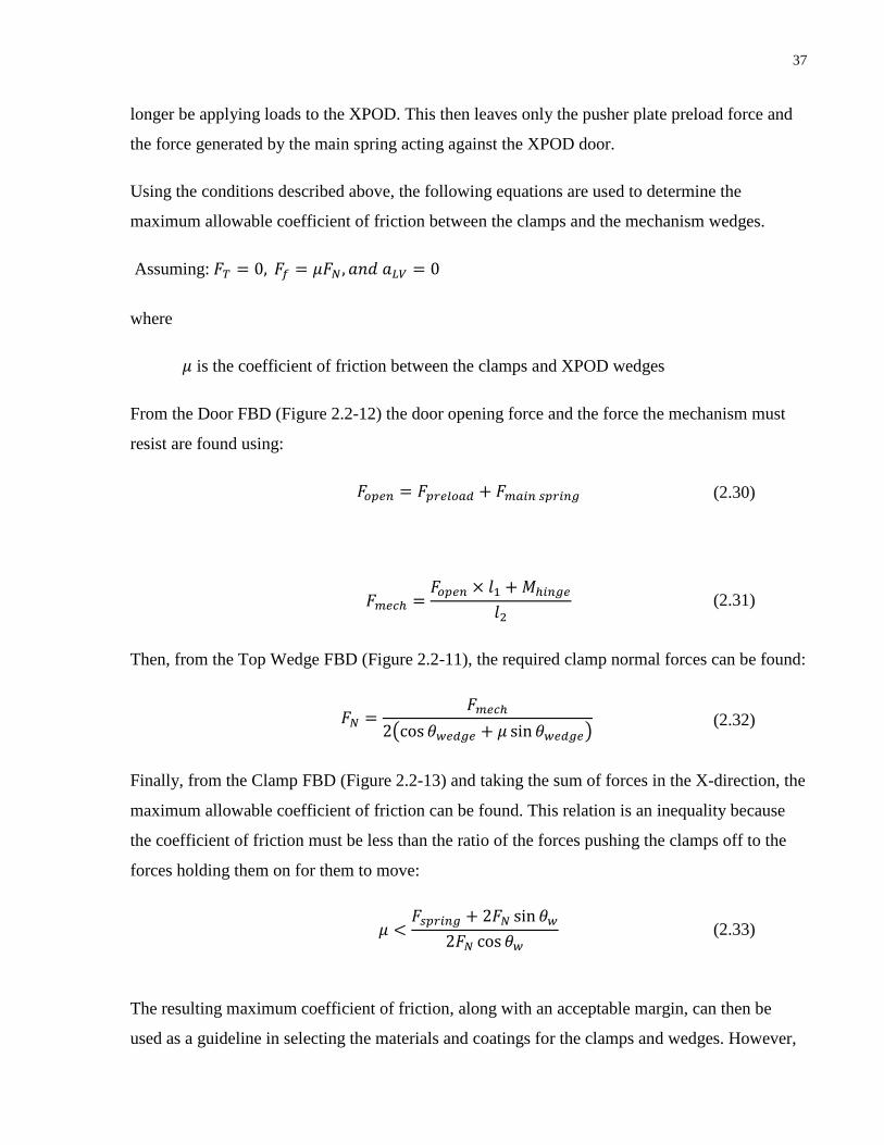
Figure 2.3-9: Stage Three Ejection Geometry Overall View ....................................................... 44
Figure 2.3-10: Stage 3 Ejection Zoom 1 ....................................................................................... 44
Figure 2.3-11: Stage 3 Ejection Zoom 2 ....................................................................................... 45 Figure 2.3-12: XPOD Deployment Steps with Pusher Plate ........................................................ 46 Figure 2.3-13: Spacecraft in Armed Configuration in Y-P Plane ................................................. 47
Figure 2.3-14: Spacecraft in Armed Configuration in X-P Plane ................................................. 48 Figure 2.3-15: XPOD Launch Rail Taper Geometry .................................................................... 48 Figure 2.4-1: +Z Tray Comparison ............................................................................................... 68 Figure 2.4-2: -Z Tray Reaction Wheel Hole Relocation ............................................................... 69 Figure 2.4-3: -Z Tray Internal Components Comparison ............................................................. 70
Figure 2.4-4: -Z Tray Sun Sensor Comparison 1 .......................................................................... 70
Figure 2.4-5: -Z Tray Sun Sensor Comparison 2 .......................................................................... 71
Figure 2.4-6: +X Panel Internal Comparison ................................................................................ 71 Figure 2.4-7: +X Panel External Comparison............................................................................... 72 Figure 2.4-8: -X Panel Internal Comparison ................................................................................. 72 Figure 2.4-9: -X Panel External Comparison ............................................................................... 73 Figure 2.4-10: +Y Panel Internal Comparison .............................................................................. 74
Figure 2.4-11: +Y Panel External Comparison............................................................................. 74

Figure 2.4-12: -Y Panel Internal Comparison ............................................................................... 75 Figure 2.4-13: -Y Panel External Comparison ............................................................................. 75 Figure 2.4-14: UHF Antenna Cutout Comparisons (Dimensions in Millimeters)........................ 76 Figure 2.4-15: +Z Panel Internal Comparison .............................................................................. 77
Figure 2.4-16: +Z Panel External Comparison ............................................................................. 77 Figure 2.4-17: +Z Panel External Isometric View ........................................................................ 78 Figure 2.4-18: -Z Panel Internal Comparison ............................................................................... 78 Figure 2.4-19: -Z Panel External Comparison .............................................................................. 79 Figure 2.5-1: NORSAT-1 Initial Bus Design ............................................................................... 79
Figure 2.5-2: Design of Payloads at Proposal Phase .................................................................... 80
Figure 2.5-3: Modified CLARA and ASR x50 Payload Volumes ............................................... 82
Figure 2.5-4: NORSAT-1 Bus Design, H27 Form Factor ............................................................ 82 Figure 2.5-5: Views of GHGSat-D during the NORSAT-1 Preliminary Design Phase [20] ....... 83 Figure 2.5-6: NORSAT-1 PDR Bus Design Exterior Views and Rough Dimensions ................. 84 Figure 2.5-7: NORSAT-1 Exterior PDR Design View 1 ............................................................. 85
Figure 2.5-8: NORSAT-1 Exterior PDR Design View 2 ............................................................. 85 Figure 2.5-9: NORSAT-1 Interior PDR Bus Design .................................................................... 86
Figure 2.5-10: Langmuir Probe Clearances from PDR Design .................................................... 87 Figure 2.5-11: NORSAT-1 Modified PDR Design ...................................................................... 88 Figure 3.2-1: Overall Top View of FEM ...................................................................................... 90
Figure 3.2-2: Overall Bottom View of FEM ................................................................................ 90
Figure 3.2-3: Bottom View of FEM with Constraints Shown ...................................................... 91 Figure 3.3-1: Image of First Natural Frequency ........................................................................... 93 Figure 3.3-2: Image of Second Natural Frequency ....................................................................... 93
Figure 3.3-3: Image of Third Natural Frequency .......................................................................... 94 Figure 3.3-4: Overall Nodal Displacement of Bus Components for -Z Loading Case ................. 95
Figure 3.3-5: Overall Panel Stress Distribution Image from -Z Loading Case ............................ 95 Figure 3.3-6: Bottom View of -Z Panel Stress Distribution from -Z Loading Case .................... 96 Figure 3.3-7: Image of Highest Stress Component from -Z Loading Case .................................. 96
Figure 4.1-1: XPOD Triple Vibration Test Mounting Holes and Axes ........................................ 98 Figure 4.1-2: Accelerometer Placement Image 1 ......................................................................... 99
Figure 4.1-3: Accelerometer Placement Image 2 ......................................................................... 99 Figure 4.1-4 – 50g Shock Test Waveform .................................................................................. 102 Figure 4.1-5: XPOD From +Z View Example Image ................................................................. 103 Figure 4.1-6: Measurement Example Image ............................................................................... 103
Figure 4.2-1: Overall Test Setup ................................................................................................. 109 Figure 4.2-2: Cord Looping Example ......................................................................................... 112 Figure 4.2-3: Spacecraft in XPOD Orientation ........................................................................... 113

1
Introduction
The work that was completed for this thesis focused on developing the mechanical aspects of
nanosatellites and microsatellites, along with developing their separation systems. Specifically,
work was completed for the Space Flight Laboratory’s in-house separation system (i.e. the
XPOD), the MiniMags feasibility study, the EV9 mission, and the NORSAT-1 mission. This
chapter will serve to introduce each of these projects along with introducing the objectives that
were set out in relation to these projects.
1.1 The Exoadaptable Pyroless Deployer
1.1.1 Separation Systems Overview
The eXoadaptable PyrOless Deployer (XPOD) is the nano-satellite and micro-satellite separation
system that has been developed at the Space Flight Laboratory (SFL). There are currently five
flight qualified XPOD designs at SFL. Table 1 gives an overview of each of the qualified XPOD
designs at SFL.
Table 1: Overview of Qualified XPOD Designs
XPOD Designation Qualified Maximum Mass Designed Spacecraft Dimensions
Single 1.33 kg 100 mm x 100 mm x 113.5 mm
Double 2.66 kg 100 mm x 100 mm x 227 mm
Triple 3.5 kg 100 mm x 100 mm x 340.5 mm
GNB 7.5 kg 200 mm x 200 mm x 200 mm
H27 10 kg 270 mm x 270 mm x 270 mm

2
Images of each of the currently qualified XPODs are shown in Figure 1.1-1:
Figure 1.1-1: Images of Currently Qualified XPODs
The XPOD uses the push-out deployment method, which simply means that the separation
system fully contains its associated spacecraft and upon receiving the deployment command a
door is allowed to open and a spring pushes the spacecraft out. This method is typically used for
nano-satellites and micro-satellites because their structures do not have much available surface
area or the structural rigidity to allow for more discretized hold down methods. Other examples
of separation systems that use the push-out method are the Poly-Picosatellite Orbital Deployer
(P-POD) from the California Polytechnic State University and the Tokyo Picosatellite Orbital
Deployer (T-POD) from Tokyo University [1]. Most of the variations between these deployers
stem from their available form factors, and the door actuation mechanisms that are used.
Finally, as mentioned above, discretized deployment methods are also used for spacecraft
interfaces with launch vehicles. These methods are typically for larger spacecraft since total
spacecraft containment would require an impractically large and massive push-out deployer

3
structure. These methods will either have features built into the main structure of the spacecraft,
or an additional separation system adapter component mounted to the spacecraft structure, which
are used as the interface points between the launch vehicle and spacecraft. The actuation method
for these systems may be pyrotechnics, or a mechanically actuated system. An example of a
system that uses and separation system adapter component, and is mechanically actuated, is the
Motorized Lightband Mark II from Planetary System Corporation [2].
1.1.2 Exoadaptable Pyroless Deployer Operation Method
As previously mentioned, the XPOD uses the push-out deployment method. This means that to
arm the XPOD, a spacecraft will be inserted, which causes an internal spring to be compressed
and to store potential energy. This spring is attached to the bottom panel of the XPOD and to a
“pusher plate” on which the spacecraft rests. Figure 1.1-2 details several of the internal XPOD
components.
Figure 1.1-2: XPOD with Labelled Internal Components
4
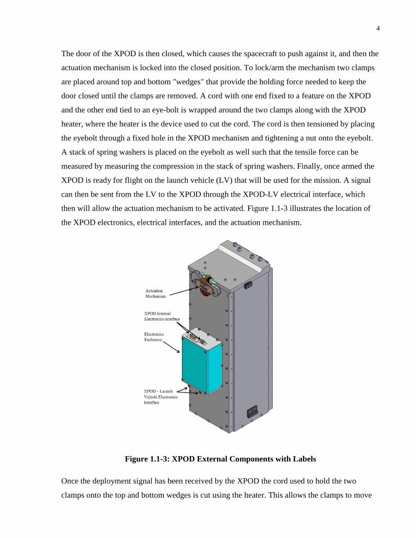
The door of the XPOD is then closed, which causes the spacecraft to push against it, and then the
actuation mechanism is locked into the closed position. To lock/arm the mechanism two clamps
are placed around top and bottom "wedges" that provide the holding force needed to keep the
door closed until the clamps are removed. A cord with one end fixed to a feature on the XPOD
and the other end tied to an eye-bolt is wrapped around the two clamps along with the XPOD
heater, where the heater is the device used to cut the cord. The cord is then tensioned by placing
the eyebolt through a fixed hole in the XPOD mechanism and tightening a nut onto the eyebolt.
A stack of spring washers is placed on the eyebolt as well such that the tensile force can be
measured by measuring the compression in the stack of spring washers. Finally, once armed the
XPOD is ready for flight on the launch vehicle (LV) that will be used for the mission. A signal
can then be sent from the LV to the XPOD through the XPOD-LV electrical interface, which
then will allow the actuation mechanism to be activated. Figure 1.1-3 illustrates the location of
the XPOD electronics, electrical interfaces, and the actuation mechanism.
Figure 1.1-3: XPOD External Components with Labels
Once the deployment signal has been received by the XPOD the cord used to hold the two
clamps onto the top and bottom wedges is cut using the heater. This allows the clamps to move

5
off of the wedges and the door to open. Figure 1.1-4 points out the parts of the mechanism that
are of importance for this step in the deployment process.
Figure 1.1-4: Parts of the XPOD Mechanism with Labels
Once the door is open the stored spring energy that was generated when the spacecraft was
placed into the XPOD pushes the spacecraft out through the open door area. The energy from the
spring is converted into the kinetic energy of the spacecraft, which dictates what the final relative
velocity of the spacecraft will be. An illustration of the arming events is shown in Figure 1.1-5
and for more information on the origination of the design of the XPOD see [3]. Finally, the side
panel of the XPOD is hidden in Figure 1.1-5 to aid in illustrating the arming steps, but in reality
it is always on the XPOD.

6
Figure 1.1-5: XPOD Arming Steps
The XPOD work for this thesis was completed mostly for the XPOD Triple. This XPOD had
previously and successfully been flown for the CanX-2 mission. At the start of the thesis work,

7
the CanX-7 mission, which uses a 3U form factor bus like CanX-2, began looking into using the
XPOD Triple as their separation system. However, the CanX-7 anticipated launch mass was
approximately four kilograms, which was greater than the mass that the XPOD Triple had
previously been qualified for. Therefore, the work completed for this thesis was to determine if
this increased mass was acceptable for the XPOD Triple.
1.2 The MiniMags Feasibility Study
The MiniMags feasibility study was a project that was funded by the Canadian Space Agency
(CSA) and carried out at SFL in conjunction with the Rutherford Appleton Laboratory (RAL).
The overall objective of this partnership was to produce and test a spacecraft subsystem that
produces active space radiation shielding. This subsystem, pending the successful demonstration
of its performance, would then be used on the CSA funded Polar Communications and Weather
(PCW) mission.
The PCW mission is specifying a Molniya orbit because of its observation requirements, and it
has a total lifetime requirement of 20 years. Using metal shielding on the PCW spacecraft, the
CSA predicts an average satellite lifespan of approximately five years based on the total
radiation dose they expect and what they have deemed tolerable for their parts. The MiniMags
payload would be used to increase the lifespan of each of the spacecraft in the PCW mission by
reducing the total radiation dose per unit time, such that the overall cost associated with the
mission would be decreased.
The goal of this portion of the mission, the feasibility study, was to determine the feasibility of
flying the MiniMags payload in a microsatellite. RAL was responsible for designing the payload
for this mission, where SFL was responsible for the satellite bus that could be used to support
their payload. Following the feasibility study phase, if this mission were to proceed, the goal
would then be to demonstrate, in flight, the effectiveness of the RAL radiation shield. The
purpose of demonstrating the RAL payload is such that other large satellite missions could use
the technology to increase the lifespans of their busses, without excessive metal shielding.
According to [4] the Van Allen belts are radiation belts that exist around the Earth in two bands.
The inner Van Allen belt exists from an altitude of approximately 100 km, in some areas, to
10,000 km and contains trapped electrons along with high energy protons. The outer Van Allen

8
belt exists from approximately 13,000 km to 16,000 km and contains mostly trapped electrons.
Figure 1.2-1 shows a representative illustration of the Van Allen belts around the Earth.
Figure 1.2-1: Van Allen Belt Illustration [4]
The radiation in these belts tends to cause both short term and long term issues with spacecraft
[5]. The two main short term issues that are realized are bit flips (aka single event upsets
(SEU’s)) and latch-ups (aka single event latch-ups (SEL’s)), which are both known as single
event effects (SEE’s). A bit flip is when a radiation particle changes the state of a bit in memory.
This causes errors in memory and operation of the spacecraft. A latchup is when a radiation
particle encounters a gate in a circuit and causes it to latch in a state where it allows the flow of
current when current is not supposed to flow. This can permanently damage electronics and
careful design must be implemented to counteract these effects, along with the errors that can
occur in memory from bit flips.
The long term effects of radiation are that electronics tend to degrade over time when exposed
[6]. Typically, an electronic component can endure a certain total exposure to radiation before it
is not reliable anymore. Testing of this effect on the ground is difficult because the true radiation
environment in space is not very reproducible, so instead of producing absolute correlations
between radiation and part life, comparative testing is carried out [7]. Comparative testing does
not necessarily reveal how long a part will last in space, but it can determine how well,
relatively, two parts work when exposed to the same type of radiation. Special materials can also

9
be used to increase resistance to radiation degradation, but typically these parts are more
expensive and can be out of reach of some missions.
The MiniMags mission was unique compared to other SFL missions because of its planned orbit,
along with the different type of payload. Typically, SFL satellites operate in Low Earth Orbit
(LEO), but the MiniMags demonstrator would either operate in a Highly Elliptical Orbit (HEO)
or Molniya Orbit. These orbits then require different launch vehicles in some cases because not
all LEO launch vehicles can deliver to these more energetic orbits. Also, the thermal and
radiation environments in these orbits are different than LEO because of their distances from
Earth and different eclipse periods [8].
SFL missions typically have either optical payloads, or communications based payloads. For
example, the AISSat satellites at SFL all carry Automatic Identification System (AIS) receivers.
These busses can receive the AIS signals from ships around the world, and then transmit them
back to Earth for terrestrial use. The BRITE satellites at SFL carry optical instruments for
observing stars. Both of these missions carry unique requirements for pointing accuracy, power,
mass, and operational characteristics. The magnetic shield payload therefore also carries unique
requirements in these areas when compared to optical and communications payloads.
Lastly, the MiniMags feasibility study kicked off after the work for this thesis began and was
finished before the thesis work completed. Therefore, this thesis covered all of the mechanical
design aspects that were completed for the MiniMags feasibility study.
1.3 The EV9 Mission
The EV9 mission is an Automatic Identification System (AIS) signal detection mission that is
being carried out by SFL along with exactEarth Limited. Originally, the EV9 mission scope was
such that it had two separate payloads, along with an original set of attitude requirements and
volume constraints. However, due to contractual changes the original scope was changed, which
led to the EV9 mission being partially re-designed.
The original mission, now called EV9-A, was designed to contain two payloads related to AIS
signal detection and processing. It was also designed to use hysteresis rods along with permanent

10
magnets for attitude control. Deployable UHF antennas were the required antennas for the uplink
from a ground station due to the volume constraints imposed on the EV9-A mission by the
launch provider.
The new mission, EV9, has had changes to the payload, attitude control system, and UHF
antennas compared to EV9-A. EV9 has only one payload and has a three-axis attitude control
system, which contains three reaction wheels along with three orthogonal magnetorquers. The
UHF antennas on EV9 are fixed, which means that they are in their flight configuration during
ascent on the launch vehicle. Both missions were scoped to use a GNB satellite bus design.
Aside from comparing EV9-A and EV9, one difference between both EV9 missions and other
SFL AIS satellites is that EV9 uses a deployable VHF antenna, where the others use a fixed VHF
antenna for AIS signal detection. The reason for this difference is due to launch provider volume
requirements imposed on the EV9 mission, which requires a deployable VHF antenna solution.
When work for the EV9 mission began, as part of this thesis, the requirements for the new EV9
bus were already established. Along with that, other GNB bus designs that met portions of these
requirements had already been designed for other mission. Therefore, the EV9 mission was able
to draw from these other missions in creating its bus design and this reduced the analysis that
was required since the designs that were drawn from had already been qualified. Finally, by the
end of the thesis work, the flight EV9 bus had been fully assembled and testing was completed
that verified the bus met all of its design requirements.
1.4 The NORSAT-1 Mission
Norwegian Satellite – 1 (NORSAT-1) is a mission being carried out at SFL to design a bus that
will contain three different Norwegian payloads. The three payloads are: 1) The Compact
Lightweight Absolute Radiometer (CLARA), 2) Langmuir probes, and 3) an AIS signal
detection payload. In what follows, the requirements for each of the payloads can be found in
[9]. An exterior view of the bus design from the Preliminary Design Review (PDR) stage of the
mission is shown in Figure 1.4-1:

11
Figure 1.4-1: NORSAT-1 PDR Stage Bus Design Overview
The CLARA payload is a scientific instrument that will be used to determine the total solar
irradiance of the Sun. This instrument is the primary payload in the NORSAT-1 mission and will
take operational precedence over the other payloads. The CLARA payload contains
measurement cavities that must be exposed, unshadowed, and must be pointed at the Sun with
±0.5 degree, 3σ, to carry out its scientific measurements. These cavities must also be held at a
constant temperature, with a maximum drift of 0.1 Celsius per hour, while the measurements are
being taken.
The Langmuir probe instrument is the secondary payload for the NORSAT-1 mission. This
instrument will measure the plasma around the Earth at a higher resolution compared to other
Langmuir probe instruments that have been flown in space. This instrument uses four probes that
are held at different electrical potentials outside of the bus, and measures the electrical
characteristics of the plasma near the spacecraft as the bus moves through the plasma around the
Earth. Most other Langmuir probe instruments use a probe that sweeps through different
voltages, but due to the time it takes for this sweep and the high velocities of orbiting satellites,
spatial resolutions of these measurements tend to be on the order of one kilometer. Since the
probes in this mission are held at constant voltages, sampling rates are much higher and give

12
spatial resolutions of the measurements on the order of one meter. These probes must be held
outside of the plasma sheath that forms around the bus as it goes through its orbit, which places
constraints on the orientation of the probes relative to the orbit.
The AIS signal detection payload (the ASR x50) is the tertiary payload for the NORSAT-1
mission. It is similar to the payloads used in the AISSats and on EV9, however it is of higher
performance. This payload is expected to be able to detect the AIS signals from more ships than
the AIS receivers in AISSat and EV9 in high ship density areas. This payload requires a
minimum of two VHF antennas for its AIS detection algorithms to work properly, but can use up
to four antennas. These antennas must be orthogonal to each other when mounted to a spacecraft,
and they must be orthogonal to the Langmuir probes in the NORSAT-1 mission. The baseline for
the VHF antennas is to use the deployable VHF antennas that are used in the EV9 mission.
The NORSAT-1 portion of the thesis work began at the kick-off of the mission. At this point
there was an existing bus design that was submitted as part of the proposal for SFL to obtain the
mission. This design was worked with, along with accounting for the evolving designs of each of
the payloads, to lead into the design of the bus that was generated for the thesis work.
1.5 Thesis Objectives
The objectives for the thesis work were associated with developing the mechanical aspects of
XPODs, the MiniMags feasibility study, the EV9 mission, and the NORSAT-1 mission. These
objectives were approached with the use of engineering design, computer simulation, and
physical testing such that they could be successfully fulfilled.
The objectives for XPODs were to first determine, with the use of analysis and testing, if the
XPOD Triple was compatible with a spacecraft mass of four kilograms. Once compatibility was
determined, then procurement of the XPOD Triple structure was to be completed such that the
CanX-7 mission had a separation system for their satellite.
The objectives for the MiniMags feasibility study were to determine, from a mechanical
standpoint, if the MiniMags payload could be supported in a nanosatellite or microsatellite. This
involved determining the mechanical requirements for the payload by consulting with the

13
payload manufacturer. Following this, plausible bus designs were proposed to the manufacturer
and they selected the most suitable design. Iterations were then completed to come up with a
design that was more tailored to the specific MiniMags payload requirements. Documentation of
the final design was created and the study was completed.
For the EV9 mission, the objectives were to merge the existing bus designs into the new EV9 bus
design, procure the newly created design, assemble the bus, and then test the assembled system.
These objectives were all completed by the time the thesis work was completed.
Finally, for the NORSAT-1 mission, the objective was to iterate on the bus deign that was used
for the mission proposal. This was to be completed based upon the evolving designs of the
payloads and as the bus design matured. The work for this mission was then handed off to
another SFL student such that the design could be further matured.

14
Mechanical Systems Design
2.1 Derivation of Mechanical Requirements
Since a major part of the mechanical requirements for a spacecraft are associated with the
loading that the spacecraft must withstand during launch, an investigation into what the loading
will be was required. The XPOD Triple, MiniMags, and NORSAT-1 did not know what launch
vehicle they would be flown on when they were being designed. Therefore, they were designed
to be compatible with a range of possible launch vehicles.
To be compatible with a launch vehicle from a mechanical standpoint a spacecraft and its
separation system must both survive the expected loading of the LV without failure, along with
exhibiting a certain degree of stiffness, which is quantified by the first natural frequency of the
spacecraft. Table 2 summarizes some of the relevant launch vehicle expected loading conditions,
along with their stiffness requirements:
Table 2: Launch Vehicle Mechanical Environment Summary
Vehicle Name
PSLV SOYUZ Ariane 5
Reference Document [10] [11] [12]
Dynamic Loading
Requirement
7g compression/
3g tension
6.5g
compression/
2.34g tension
2g compression/
2g tension
Dynamic Loading Factor of
Safety Requirement
1.25 1.3 1.1
Maximum Power Spectral
Density for Random
Vibration
6.7 GRMS 11.2 GRMS Not Listed
15
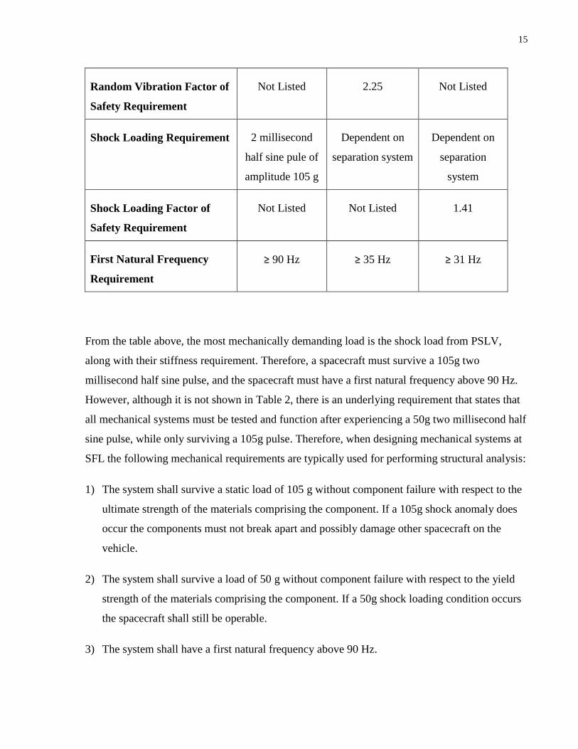
Random Vibration Factor of
Safety Requirement
Not Listed 2.25 Not Listed
Shock Loading Requirement 2 millisecond
half sine pule of
amplitude 105 g
Dependent on
separation system
Dependent on
separation
system
Shock Loading Factor of
Safety Requirement
Not Listed Not Listed 1.41
First Natural Frequency
Requirement
≥ 90 Hz ≥ 35 Hz ≥ 31 Hz
From the table above, the most mechanically demanding load is the shock load from PSLV,
along with their stiffness requirement. Therefore, a spacecraft must survive a 105g two
millisecond half sine pulse, and the spacecraft must have a first natural frequency above 90 Hz.
However, although it is not shown in Table 2, there is an underlying requirement that states that
all mechanical systems must be tested and function after experiencing a 50g two millisecond half
sine pulse, while only surviving a 105g pulse. Therefore, when designing mechanical systems at
SFL the following mechanical requirements are typically used for performing structural analysis:
1) The system shall survive a static load of 105 g without component failure with respect to the
ultimate strength of the materials comprising the component. If a 105g shock anomaly does
occur the components must not break apart and possibly damage other spacecraft on the
vehicle.
2) The system shall survive a load of 50 g without component failure with respect to the yield
strength of the materials comprising the component. If a 50g shock loading condition occurs
the spacecraft shall still be operable.
3) The system shall have a first natural frequency above 90 Hz.

16
When validating these requirements, both a Finite Element Model (FEM) and physical tests are
used. The 105g loading condition is only analyzed with the use of a FEM because the PSLV
provider believes this loading condition is a highly unlikely event on the launch vehicle, which
can lead to a high degree of overdesign of spacecraft components. Therefore, since this load will
likely permanently damage the structure during physical testing, it is not required. However, both
a FEM and physical testing with the 50g load are completed since this loading condition is said
to be much more likely to occur.
Thorough inspections along with accelerometers are used to determine the performance of the
test article during physical tests. To determine the natural frequencies of the structure, following
a prediction with the use of a FEA, a low amplitude sine wave is input into the structure using a
vibration table, and then accelerometers measure the accelerations of different points on the
structure. When these measured accelerations exhibit resonance with respect to the input load,
then the natural frequencies are determined and compared against the requirement. The results
are also compared against the results from the FEA that was previously completed for validation
purposes.
Physical tests are also completed to ensure that the dynamic and random vibration loads from
launch vehicles are tolerated by the structures that are tested. However, because their amplitudes
are less severe than both the 50g and 105g case they are not the main design drivers for the
structure. More information on the random and dynamic loading tests can be found in [13].

17
2.2 XPOD Mechanical Design
2.2.1 Mechanical Design of the XPOD Mechanism, Internal Preload and Main Spring
The XPOD Triple was originally designed to carry a 3.5 kg spacecraft, but the CanX-7 satellite
that will use a XPOD Triple has a currently predicted mass between 3.5 kg and 4 kg. Therefore,
a decision was made to increase the mass capacity of the XPOD Triple to 4 kg. This requires that
there be additional investigation into the design of the mechanism for the XPOD, along with its
main spring. The expected modification to the mechanism will be that the preload in the cord
that is used to hold the mechanism shut must be modified to be appropriate for the four kilogram
spacecraft. The main spring must also be made to contain more energy since the same ejection
velocity is desired and the spacecraft will be more massive, which will require more kinetic
energy.
The mechanism preload and main spring designs are also important to other XPODs that were
developed during this thesis activity. One other aspect that was not mentioned above is the
design of the pusher plate preload. This preload is designed to allow for practical machining
tolerances when manufacturing an XPOD, along with helping to maintain contact between a
spacecraft, the XPOD door, and the pusher plate when the system experiences loading in the
XPOD deployment direction.
Sections 2.2.2 through 2.2.6 will give an overview of the XPOD mechanism working principal
along with the details of how the other mechanical aspects of the XPOD are designed.
2.2.2 XPOD Mechanism Overview
The XPOD mechanism is used to both lock, and release the door of the XPOD with the use of a
clamp-wedge interference system (See Figure 2.2-1). The clamps are held together by a cord,
and upon the deployment signal being received by the XPOD electronics a heater is activated
that burns through the cord. A simplified sequence of images shows the general working concept
of the mechanism in Figure 2.2-2.

18
Figure 2.2-1: Isometric View of XPOD Triple Mechanism before Deployment
1) Mechanism Before Deployment 2) Cord cut by heater.
3) Clamps begin to move off of wedges. 4) Clamps fully moved off of wedges.
5) XPOD door allowed to open freely
Figure 2.2-2: Simplified XPOD Mechanism Actuation Sequence

19
The tension in the cord that is used to hold the clamps onto the wedges must be sufficient such
that the clamps do not move when the XPOD and spacecraft experience loading. This tension is
calculated using the expected worse case loading from the launch vehicle, the XPOD internal
forces, and accounting for the geometry of the mechanism components. After the tension that is
required is found then the compression that is required in the preload stack in the mechanism is
calculated.
2.2.3 Pusher Plate Preload Design
Due to tolerances in the XPOD system it is not practical to design an XPOD that when the door
is closed there are no gaps between the parts that lie between the bottom of the XPOD door and
the top of the XPOD base plate. If this was attempted it would likely result in a gap between
these parts if the tolerance stacking of the parts is too short. Alternatively, if the tolerance
stacking is too high, the XPOD door may not be able to close. Therefore to resolve this issue a
compressible, “Bellville Stack”, section is included in the stack of components between the
baseplate and door as shown in Figure 2.2-3.
This compressible section is typically a stack of spring washers that are located inside of the
XPOD pusher plate. However, in the event that the XPOD is for a CubeSat, an off-the-shelf
preload plunger is used instead of spring washers (see [3]). The total height of the components
between the door and base plate is chosen to be a height such that if the compressible section
were solid, would be too tall to fit within the door and base plate. However, once the
compressible section is compressed by a predetermined amount the door can close. After the
door is closed and the deployment mechanism is armed, the compressed section is allowed to
partially decompress, which causes it to force the spacecraft against the door. The force that is
generated is called the “preload force” and the magnitude of this force will be discussed in
Section 2.2.3.1. A section view of an XPOD pusher plate is shown in Figure 2.2-3.
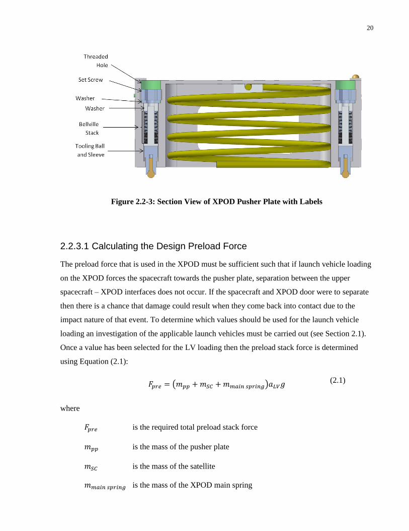
20
Figure 2.2-3: Section View of XPOD Pusher Plate with Labels
2.2.3.1 Calculating the Design Preload Force
The preload force that is used in the XPOD must be sufficient such that if launch vehicle loading
on the XPOD forces the spacecraft towards the pusher plate, separation between the upper
spacecraft – XPOD interfaces does not occur. If the spacecraft and XPOD door were to separate
then there is a chance that damage could result when they come back into contact due to the
impact nature of that event. To determine which values should be used for the launch vehicle
loading an investigation of the applicable launch vehicles must be carried out (see Section 2.1).
Once a value has been selected for the LV loading then the preload stack force is determined
using Equation (2.1):
𝐹𝑝𝑟𝑒 = (𝑚𝑝𝑝 + 𝑚𝑆𝐶 + 𝑚𝑚𝑎𝑖𝑛 𝑠𝑝𝑟𝑖𝑛𝑔)𝑎𝐿𝑉𝑔 (2.1)
where
𝐹𝑝𝑟𝑒 is the required total preload stack force
𝑚𝑝𝑝 is the mass of the pusher plate
𝑚𝑆𝐶 is the mass of the satellite
𝑚𝑚𝑎𝑖𝑛 𝑠𝑝𝑟𝑖𝑛𝑔 is the mass of the XPOD main spring

21
𝑎𝐿𝑉 is the design acceleration from the launch vehicle
𝑔 is the acceleration due to gravity
An assumed mass of the main spring may need to be used since the main spring design may not
have been completed yet. Iteration to include the actual main spring mass may be required if the
assumption is very different than the actual value that will be found in future calculations.
2.2.3.2 Bellville Stack Design
A Bellville stack is comprised of several spring washers, shims, and normal (non-spring)
washers. The shims and non-spring washers are included in the stack to increase the height of the
stack without affecting its spring constant. These stacks are used in both the XPOD mechanism
and inside the XPOD pusher plate to create compressible assemblies that allow for measured
deflections to be converted to calculated compressive forces. A stack from an XPOD GNB is
shown in Figure 2.2-4:
Figure 2.2-4: XPOD GNB Bellville Stack
The Bellville stack along with the top washer are placed over a rod type component for stability
as shown in the exploded view in Figure 2.2-5.

22
Figure 2.2-5: Exploded View of XPOD GNB Stack
To calculate the force that a single Bellville washer exerts at a given compressed height, a
process from [14] was used, which is applicable to Bellville washers with a material thickness of
two millimeters or less. Figure 2.2-6 shows a cross-section of a Bellville washer along with
important quantities:
Figure 2.2-6: Bellville Washer Diagram with Labels [14]
where
𝐷 is the outer diameter of the washer
𝑑 is the inner diameter of the washer
𝑂. 𝐻. is the overall height of the washer
ℎ is the inside height of the washer
𝑡 is the thickness of the washer material
The diameter ratio of a Bellville washer is then given by Equation (2.2):

23
𝛿 =
𝐷
𝑑 (2.2)
where
𝛿 is the diameter ratio
Following the calculation of the Bellville washer diameter ratio, Equation (2.3) is used to find
the following dimensionless calculation constant:
𝑀 =
6
𝜋 × ln(𝛿)×
(𝛿 − 1)2
𝛿2 (2.3)
where
𝑀 is the dimensionless calculation constant
The deflection of a single Bellville washer is then defined by Equation (2.4):
𝑓𝑖 = 𝑂𝐻 − 𝑂𝐻𝑖 (2.4)
where
𝑓𝑖 is the deflection that the washer has undergone
𝑂𝐻𝑖 is the compressed overall height of a spring washer
Now, with the results of Equations (2.2) to (2.4), and with knowledge about the material
properties of the washer, the force being exerted can be calculated:
𝑃𝑖 =
𝐸 × 𝑓𝑖
(1 − 𝜇2) × 𝑀 × (𝐷2)
2 × [(ℎ −𝑓𝑖
2) × (ℎ − 𝑓𝑖) × 𝑡 + 𝑡3] (2.5)
where
𝑃𝑖 is the force exerted by the washer at the given deflection
𝐸 is the Young’s modulus of the washer material
𝜇 is the Poisson’s ratio of the washer material

24
After the force that results from a single spring washer is determined, then depending on how
these washers are stacked one can determine the force of the entire Bellville stack. An example
stacking arrangement is shown in Figure 2.2-7:
Figure 2.2-7: Bellville Stacking Arrangement Example
The stack shown in Figure 2.2-7 has a total of eight spring washers. These spring washers are
arranged with two unidirectional washers in each stack, and there are a total of four “individual
stacks”. In designing a stack one must consider the desired total force, the uncompressed height,
and the compressed height. These will depend on the XPOD geometry along with the desire to
make the deflection as measurable as possible given geometric and force constraints.
To explain the measurability of the stack, typically a total stack compression is between one and
two millimeters and errors of five percent on the final compression magnitude are acceptable.
Therefore, a stack that has a larger absolute deflection to achieve the desired force will be easier
to measure and compress the desired amount.
Once a desired stack design has been selected the overall force that the stack will exert for a
given deflection is found by first calculating the height of an “individual stack”:
𝐻𝑠𝑖= (𝑂𝐻𝑖 + 𝐴 × 𝑡) (2.6)
where

25
𝐻𝑠𝑖 is the resulting individual stack height
𝐴 is the number of unidirectional washers in an individual stack
Following the calculation of the height of the “individual stacks”, the total stack height can be
found:
𝐻𝑡𝑖= 𝐵 × 𝐻𝑠𝑖
(2.7)
where
𝐻𝑡𝑖 is the resulting total stack height
𝐵 is the number of individual stacks
Finally, the total stack force and total stack deflection can be found:
𝑃𝑠𝑡𝑎𝑐𝑘𝑖= 𝐴 × 𝑃𝑖 (2.8)
𝑓𝑠𝑡𝑎𝑐𝑘𝑖= 𝐵 × 𝑓𝑖 (2.9)
where
𝑃𝑠𝑡𝑎𝑐𝑘𝑖 is the total stack force for a given stack arrangement
𝑓𝑠𝑡𝑎𝑐𝑘𝑖 is the total stack deflection for a given stack arrangement
From a practical standpoint the equations above are somewhat difficult to solve for the stack
deflection as a function of force since the force equations are given as a function of deflection.
Therefore, when designing a stack, iterations through deflections are carried out until the correct
total stack force is achieved.
Other means of verifying the stack force, such as a force sensor, may be required to verify the
results of the design. This is because of the manufacturing tolerances for the spring washers,
which lead to variability in the forces that are generated.

26
Finally, there may be situations where two different stacks will be used in series to achieve the
desired uncompressed height, stack force and stack deflection. In this case, since both stacks are
in series, they will both take the same force. Therefore, to determine the total deflection of the
stack, trial and error can be used for each stack such that the force they produce is equal to the
desired stack force. Then the deflections of both stacks can be summed to give the total
deflection.
2.2.4 Designing the Main Spring
The main spring in the XPOD stores the majority of the energy that is used to eject the spacecraft
from the XPOD once the XPOD is signaled to deploy. The process and equations used to design
this spring are taken from [15] with slight modification to the process to be more appropriate for
this application.
Step 1) Determine the energy stored in the pusher plate preload:
𝐸𝑝𝑟𝑒𝑙𝑜𝑎𝑑 =
1
2𝑘𝑝𝑟𝑒𝑙𝑜𝑎𝑑(𝑥2
2 − 𝑥12)
(2.10)
where
𝐸𝑝𝑟𝑒𝑙𝑜𝑎𝑑 is the energy stored in the pusher plate preload stacks
𝑘𝑝𝑟𝑒𝑙𝑜𝑎𝑑 is the total effective spring constant of all pusher plate preload stacks
𝑥2 is the compression of the preload stack in its armed state
𝑥1 is the compression of the preload stack in its unarmed state
Step 2) Determine the energy required to eject the spacecraft at the desired ejection velocity:
𝐸𝑑𝑒𝑝𝑙𝑜𝑦 =
1
2(𝑚𝑆𝐶 + 𝑚𝑝𝑝)𝑣𝑓
2 + 𝜇𝑚𝑆𝐶𝑔𝑙𝑓 − 𝐸𝑝𝑟𝑒𝑙𝑜𝑎𝑑 (2.11)
where
𝐸𝑑𝑒𝑝𝑙𝑜𝑦 is the energy required to deploy the spacecraft
𝑣𝑓 is the desired exit velocity

27
𝜇 is the coefficient of friction between the XPOD rails and the spacecraft
𝑙𝑓 is the length that the spacecraft will be in contact with the XPOD rails
𝑔 is the acceleration due to gravity
𝑚𝑆𝐶 is the spacecraft mass
𝑚𝑝𝑝 is the pusher plate mass
Equation (2.11) assumes that there are frictional losses that are equal to those that would exist on
Earth. This assumption is used to be conservative in the analysis, but is not necessarily
physically representative.
Step 3) Determine the compressed length of the spring (𝐿𝑐), which is a function of the XPOD
geometry. When the spring is compressed it will be the total length that is between the top of
the XPOD base plate, and the bottom of the pusher plate when the pusher plate preloads are
compressed.
Step 4) Select a free length for the spring (𝐿𝑜).This value must be small enough such that the
pusher plate does not rest outside the XPOD when the spring is at its free length.
Step 5) Determine the required spring constant for the main spring to achieve the desired energy
storage for the deployment:
𝑘𝑠𝑝𝑟𝑖𝑛𝑔 =
2𝐸𝑑𝑒𝑝𝑜𝑦
(𝐿𝑜 − 𝐿𝑐)2 (2.12)
where
𝑘𝑠𝑝𝑟𝑖𝑛𝑔 is the required spring constant
Step 6) Based on an assumed wire diameter, calculate the mean diameter of the spring:
𝐷 = 𝑂𝐷 − 𝑑 (2.13)
where
𝐷 is the mean diameter of the spring
𝑂𝐷 is the outer diameter of the spring and is a function of XPOD geometry

28
𝑑 is the assumed wire diameter
Step 7) Determine the force in the spring when it is at its compressed length:
𝐹𝑐 = 𝑘𝑠𝑝𝑟𝑖𝑛𝑔(𝐿𝑜 − 𝐿𝑐) (2.14)
where
𝐹𝑐 is the force exerted by the spring at its compressed length
Step 8) Calculate the spring index and the stress concentration factor:
𝐶 =
𝐷
𝑑 (2.15)
𝐾𝐵 =
4𝐶 + 2
4𝐶 − 3 (2.16)
where
𝐶 is the spring index
𝐾𝐵 is the stress concentration factor
It is best if 4 ≤ 𝐶 ≤ 12 (See [15]). If the spring index is too small the springs are difficult to
manufacture. If the spring index is too large then there may be packaging issues since the springs
tend to easily tangle. However, since low quantities of these springs are purchased for XPODs
the issue of tangling is not of concern and 𝐶 ≥ 4 is the driving constraint.
Step 9) Calculate the number of active coils in the spring (Used in future calculations in the
spring design process):
𝑁𝑎 =
𝐺𝑑4
8𝐷3𝑘𝑠𝑝𝑟𝑖𝑛𝑔 (2.17)
where
𝑁𝑎 is the number of active coils in the spring
𝐺 is the Shear Modulus of the spring material

29
Step 10) Check if the design of the spring is satisfactory with respect to its resulting
geometry and stresses. First calculate the solid length of the spring:
𝐿𝑠 = 𝑑(𝑁𝑎 − 1) (2.18)
where
𝐿𝑠 is the solid length of the spring
The solid length must be greater than the compressed length (𝐿𝑐) determined in Step 3). If it is
not, then a new free length (𝐿𝑜) must be set and a new iteration started. If the design is still
satisfactory, using the solid length, calculate the spring’s solid force:
𝐹𝑠 = 𝑘𝑠𝑝𝑟𝑖𝑛𝑔(𝐿𝑜 − 𝐿𝑠) (2.19)
where
𝐹𝑠 is the force the spring exerts at its solid length
Using the solid force and other geometry, calculate the shear stress in the spring at its solid
length:
𝜏𝑠 = 𝐾𝐵 ×
8𝐹𝑠𝐷
𝜋𝑑3 (2.20)
where
𝜏𝑠 is the shear stress in the spring at its solid length
The factor of safety for the spring at its solid length can then be found:
𝑛𝑠 =
𝑆𝑠𝑦
𝜏𝑠 (2.21)
where
𝑛𝑠 is the factor of safety of the spring with respect to its shear yield strength
𝑆𝑠𝑦 is the shear yield strength of the spring material
A simplification can be made that assumes that the shear yield strength of the spring material is
equal to 45 percent of the spring’s ultimate tensile strength [15].

30
Another important quantity that should be determined is the fractional overrun of the spring. This
value is a measure of how close the compressed force, which is the operational force of the
spring, is to the solid force of the spring. If the solid force is within 15 percent of the compressed
force, with respect to the compressed force, then the spring may behave in a non-linear manner
and should be used as a design constraint [15]. The factional overrun is calculated using:
𝜉 =
𝐹𝑠
𝐹𝑐− 1 (2.22)
where
𝜉 is the fractional overrun
Finally, the critical free length of the spring is calculated. This value must be greater than the
free length of the spring selected in Step 4) or else the spring may be unstable and buckle when
compressed. The critical free length is calculated using:
𝐿𝑐𝑟 =𝜋𝐷
𝛼[2(𝐸 − 𝐺)
2𝐺 + 𝐸]
12
(2.23)
where
𝐿𝑐𝑟 is the critical free length of the spring
𝛼 is the spring end constraint (𝛼 = 0.5) for XPODs
The free length of the spring (𝐿𝑜) from Step 4) is the variable used for iteration for a given wire
diameter. A spreadsheet can be set up that calculates all of the required values for a given spring
for a given free length along with performing all of the checks in Step 10). If a free length for the
given wire diameter passes all of the checks in Step 10) then the spring can be used for the
XPOD. If not, then a different wire diameter should be used and the process repeated until a
suitable design is found.

31
2.2.5 Determining the Required Tension in the Mechanism Cord
The first step in determining how much tension is required in the mechanism cord to prevent the
clamps from coming off is to determine the forces that are trying to open the XPOD door when
the XPOD is in an armed and LV loaded state. Figure 2.2-8 shows a simplified view of an XPOD
door and Figure 2.2-9 shows a free body diagram (FBD) that results from the expected loading
condition.
Figure 2.2-8: Simplified View of a XPOD GNB Door
Figure 2.2-9: Door Free Body Diagram
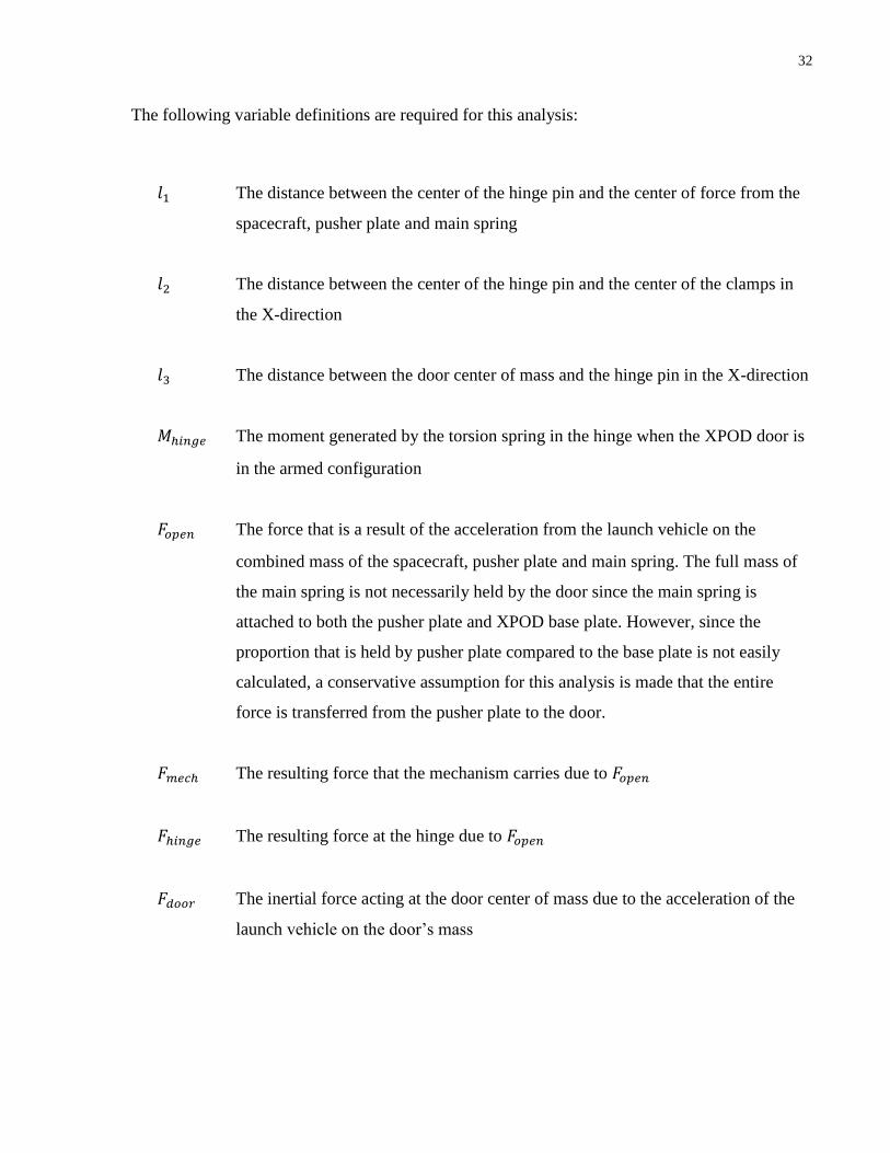
32
The following variable definitions are required for this analysis:
𝑙1 The distance between the center of the hinge pin and the center of force from the
spacecraft, pusher plate and main spring
𝑙2 The distance between the center of the hinge pin and the center of the clamps in
the X-direction
𝑙3 The distance between the door center of mass and the hinge pin in the X-direction
𝑀ℎ𝑖𝑛𝑔𝑒 The moment generated by the torsion spring in the hinge when the XPOD door is
in the armed configuration
𝐹𝑜𝑝𝑒𝑛 The force that is a result of the acceleration from the launch vehicle on the
combined mass of the spacecraft, pusher plate and main spring. The full mass of
the main spring is not necessarily held by the door since the main spring is
attached to both the pusher plate and XPOD base plate. However, since the
proportion that is held by pusher plate compared to the base plate is not easily
calculated, a conservative assumption for this analysis is made that the entire
force is transferred from the pusher plate to the door.
𝐹𝑚𝑒𝑐ℎ The resulting force that the mechanism carries due to 𝐹𝑜𝑝𝑒𝑛
𝐹ℎ𝑖𝑛𝑔𝑒 The resulting force at the hinge due to 𝐹𝑜𝑝𝑒𝑛
𝐹𝑑𝑜𝑜𝑟 The inertial force acting at the door center of mass due to the acceleration of the
launch vehicle on the door’s mass

33
The following equations are used in finding force that the mechanism carries:
𝐹𝑜𝑝𝑒𝑛 = (𝑚𝑠𝑐 + 𝑚𝑝𝑝 + 𝑚𝑠𝑝𝑟𝑖𝑛𝑔)𝑎𝐿𝑉𝑔 + 𝐹𝑝𝑟𝑒𝑙𝑜𝑎𝑑 + 𝐹𝑚𝑎𝑖𝑛 𝑠𝑝𝑟𝑖𝑛𝑔 (2.24)
𝐹𝑑𝑜𝑜𝑟 = 𝑚𝑑𝑜𝑜𝑟𝑎𝐿𝑉𝑔 (2.25)
𝐹𝑚𝑒𝑐ℎ =
𝐹𝑜𝑝𝑒𝑛𝑙1 + 𝑀ℎ𝑖𝑛𝑔𝑒 + 𝐹𝑑𝑜𝑜𝑟𝑙3
𝑙2 (2.26)
where
𝑚𝑠𝑐 is the mass of the contained spacecraft
𝑚𝑝𝑝 is the XPOD pusher plate mass
𝑚𝑠𝑝𝑟𝑖𝑛𝑔 is the mass of the main spring
𝑎𝐿𝑉 is the acceleration of the launch vehicle acting on the contained mass
(assuming worst case orientation of the XPOD).
𝐹𝑝𝑟𝑒𝑙𝑜𝑎𝑑 is the XPOD pusher plate preload force
𝐹𝑚𝑎𝑖𝑛 𝑠𝑝𝑟𝑖𝑛𝑔 is the force due to the XPOD when it is in its armed configuration
𝑚𝑑𝑜𝑜𝑟 is the mass of the XPOD door
𝑔 is the acceleration due to gravity
After the force that the mechanism must resist is found, then determining the forces within the
mechanism can begin. A FBD of the XPOD mechanism is shown in Figure 2.2-10:
Figure 2.2-10: FBD of Mechanism without Internal Forces
34
where
𝐹𝑇 is the required tension in the mechanism cord
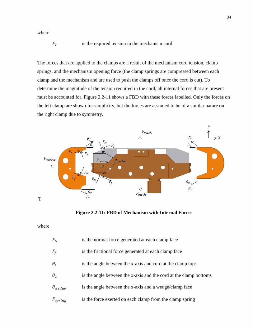
The forces that are applied to the clamps are a result of the mechanism cord tension, clamp
springs, and the mechanism opening force (the clamp springs are compressed between each
clamp and the mechanism and are used to push the clamps off once the cord is cut). To
determine the magnitude of the tension required in the cord, all internal forces that are present
must be accounted for. Figure 2.2-11 shows a FBD with these forces labelled. Only the forces on
the left clamp are shown for simplicity, but the forces are assumed to be of a similar nature on
the right clamp due to symmetry.
T
Figure 2.2-11: FBD of Mechanism with Internal Forces
where
𝐹𝑁 is the normal force generated at each clamp face
𝐹𝑓 is the frictional force generated at each clamp face
𝜃1 is the angle between the x-axis and cord at the clamp tops
𝜃2 is the angle between the x-axis and the cord at the clamp bottoms
𝜃𝑤𝑒𝑑𝑔𝑒 is the angle between the x-axis and a wedge/clamp face
𝐹𝑠𝑝𝑟𝑖𝑛𝑔 is the force exerted on each clamp from the clamp spring
35
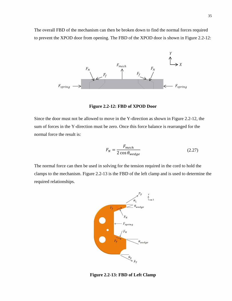
The overall FBD of the mechanism can then be broken down to find the normal forces required
to prevent the XPOD door from opening. The FBD of the XPOD door is shown in Figure 2.2-12:
Figure 2.2-12: FBD of XPOD Door
Since the door must not be allowed to move in the Y-direction as shown in Figure 2.2-12, the
sum of forces in the Y-direction must be zero. Once this force balance is rearranged for the
normal force the result is:
𝐹𝑁 =
𝐹𝑚𝑒𝑐ℎ
2 cos 𝜃𝑤𝑒𝑑𝑔𝑒 (2.27)
The normal force can then be used in solving for the tension required in the cord to hold the
clamps to the mechanism. Figure 2.2-13 is the FBD of the left clamp and is used to determine the
required relationships.
Figure 2.2-13: FBD of Left Clamp

36
The angles of the tension forces in the FBD can vary for each model of the XPOD. These angles
can also be equal to zero, but they are still included in the following analysis such that the
equations can be applied to a variety of XPODs. One assumption with these angles, which was
made because of the geometry of all XPODs that have been currently designed, is that the angles
formed at the tops of both clamps are the same, and the same applies for the angles at the
bottoms.
Based on the FBD in Figure 2.2-13, and summing the forces in the X-direction, the following
result for the required tension is found:
𝐹𝑇 =
𝐹𝑠𝑝𝑟𝑖𝑛𝑔 + 2𝐹𝑁 sin 𝜃𝑤𝑒𝑑𝑔𝑒 − 2𝐹𝑓 cos 𝜃𝑤𝑒𝑑𝑔𝑒
cos 𝜃1 + cos 𝜃2 (2.28)
One assumption that is made when finding the required tension is that the frictional forces do not
aid in holding the clamps onto the XPOD. This assumption is used to increase the conservative
nature of the analysis and yields Equation (2.29), which is used for finding the tension in the
XPOD mechanism cord:
𝐹𝑇 =
𝐹𝑠𝑝𝑟𝑖𝑛𝑔 + 2𝐹𝑁 sin 𝜃𝑤
cos 𝜃1 + cos 𝜃2 (2.29)
Using the tension force found in Equation (2.29), along with the Bellville stack design processes
detailed in Section 2.2.3.2, a Bellville stack can then be designed for the XPOD mechanism.
Finally, a structural analysis to determine the suitability of the design of the XPOD structural
components, such as the mechanism wedges or hinge, should be completed in a separate
analysis.
2.2.6 Determining the Mechanism Jamming Conditions
Although friction is not considered when finding the required tension to hold the clamps onto the
XPOD during launch vehicle loading, it must be considered when determining an allowable
coefficient of friction between the wedges and clamps once the XPOD is signaled to deploy. For
this analysis it is assumed that the launch vehicle has already reached its final orbit and will no
37
longer be applying loads to the XPOD. This then leaves only the pusher plate preload force and
the force generated by the main spring acting against the XPOD door.
Using the conditions described above, the following equations are used to determine the
maximum allowable coefficient of friction between the clamps and the mechanism wedges.
Assuming: 𝐹𝑇 = 0, 𝐹𝑓 = 𝜇𝐹𝑁 , 𝑎𝑛𝑑 𝑎𝐿𝑉 = 0
where
𝜇 is the coefficient of friction between the clamps and XPOD wedges
From the Door FBD (Figure 2.2-12) the door opening force and the force the mechanism must
resist are found using:
𝐹𝑜𝑝𝑒𝑛 = 𝐹𝑝𝑟𝑒𝑙𝑜𝑎𝑑 + 𝐹𝑚𝑎𝑖𝑛 𝑠𝑝𝑟𝑖𝑛𝑔 (2.30)
𝐹𝑚𝑒𝑐ℎ =
𝐹𝑜𝑝𝑒𝑛 × 𝑙1 + 𝑀ℎ𝑖𝑛𝑔𝑒
𝑙2 (2.31)
Then, from the Top Wedge FBD (Figure 2.2-11), the required clamp normal forces can be found:
𝐹𝑁 =
𝐹𝑚𝑒𝑐ℎ
2(cos 𝜃𝑤𝑒𝑑𝑔𝑒 + 𝜇 sin 𝜃𝑤𝑒𝑑𝑔𝑒) (2.32)
Finally, from the Clamp FBD (Figure 2.2-13) and taking the sum of forces in the X-direction, the
maximum allowable coefficient of friction can be found. This relation is an inequality because
the coefficient of friction must be less than the ratio of the forces pushing the clamps off to the
forces holding them on for them to move:
𝜇 <
𝐹𝑠𝑝𝑟𝑖𝑛𝑔 + 2𝐹𝑁 sin 𝜃𝑤
2𝐹𝑁 cos 𝜃𝑤 (2.33)
The resulting maximum coefficient of friction, along with an acceptable margin, can then be
used as a guideline in selecting the materials and coatings for the clamps and wedges. However,

38
considerations may need to be taken to ensure that other processes of material bonding aside
from friction do not occur as a function of the coatings or materials used.
2.3 XPOD Tip Off Rate Analysis
2.3.1 Problem Definition
When a spacecraft is ejected from an XPOD, there is a resulting angular velocity for the
spacecraft. From a simplified standpoint, the main reason for this is the offset between the
XPOD pusher plate force and the center of mass of the spacecraft. This offset then creates a
torque that spins up the spacecraft, which is then subject to the geometric constraints of the
XPOD rails that limit the maximum angle the spacecraft can be rotated for a given position. It is
probable that there are other causes for the angular velocity, such as unplanned launch vehicle
rotations, or imperfections in the interface between the XPOD and spacecraft. However, these
are neglected in this analysis because they are not easily measurable and are not necessarily
controllable, which would result in the error bounds for the analysis being unpredictable.
One other assumption is that the pusher plate remains in contact with the spacecraft until the
XPOD main spring reaches its free length. Since the pusher plate is the only force acting to push
the spacecraft out of the XPOD, then the spacecraft cannot travel faster than the pusher plate.
Therefore, until the pusher plate begins to slow down relative to the spacecraft, which will only
happen once the main spring reaches its free length, they will remain in contact until that point.
This then allows the force being imparted on the spacecraft to act along the line of the geometric
center of the pusher plate for the duration that the spacecraft and pusher plate are in contact.
Finally, for this analysis, the term “block” will be used to refer to either the pusher plate and
spacecraft assembly while in contact, or to just the spacecraft. This term will be used because
similar equations and processes will be applied to either the pusher plate / spacecraft assembly or
to the spacecraft by itself, depending on the stage of the analysis.

39
2.3.2 Assumed Ejection Geometry for Limiting Angles
When a spacecraft is ejected from an XPOD, there are geometric constraints that limit the angle
that the spacecraft can rotate to, which also depend on its position. Figure 2.3-1 shows an
overview of the important geometric parameters used in determining these limits.
Figure 2.3-1: Geometry Overview for Tip-Off Rate Analysis
While the pusher plate and spacecraft are in contact it is assumed that the top corner of the
pusher plate drags against the “Top XPOD Rail”. It is also assumed that bottom spacecraft edge
drags against either the leading or outer edge of the bottom launch rail taper. This geometry will
be further explained in Sections 2.3.2.1 through 2.3.2.3.
Once the pusher plate and spacecraft have separated, then the upper corner of the spacecraft that
is still inside the XPOD will drag along the top rail. The bottom edge constraint will remain the
same as it was when the pusher plate and spacecraft were in contact. The new spacecraft
constraint is shown in Figure 2.3-2.

40
Figure 2.3-2: Geometry Overview for Tip-Off Rate Analysis
after Pusher Plate Separation
The combination of rail geometry along with the pusher plate separation event gives rise to six
different possible stages for a deployment. Each of these will be further detailed in Section
2.3.2.1 through Section 2.3.2.4.
2.3.2.1 Stage 1 Ejection Geometry
The overall geometry of the first stage of the ejection is show in Figure 2.3-3 where the red block
can represent either the spacecraft, or spacecraft and pusher plate assembly. This stage of the
ejection is characterized by the upper corner of the block dragging along the non-tapered edge of
the top XPOD rail. The bottom edge of the block drags against the leading edge of the bottom
rail taper. These two areas of importance are shown with zoomed images in Figure 2.3-4 and
Figure 2.3-5.

41
Figure 2.3-3: Stage One Ejection Geometry Overall View
Figure 2.3-4: Stage 1 Ejection Zoom 1
Figure 2.3-5: Stage 1 Ejection Zoom 2
Zoom
1
Zoom
2

42
2.3.2.2 Stage 2 Ejection Geometry
The overall geometry of the second stage of the ejection is show in Figure 2.3-6 where the red
block can represent either the spacecraft, or spacecraft and pusher plate assembly. This stage of
the ejection is characterized by the upper corner of block dragging along the non-tapered edge of
the top XPOD rail and the bottom edge of the block dragging against the outside edge of the
bottom XPOD rail taper. This stage begins once the angle that the block has rotated exceeds the
angle of the taper in the XPOD rail and will exist depending on the geometry of the spacecraft,
XPOD rails, and the clearances between these components. These two areas of importance are
shown with zoomed images in Figure 2.3-7 and Figure 2.3-8.
Figure 2.3-6: Stage Two Ejection Geometry Overall View
Figure 2.3-7: Stage 2 Ejection Zoom 1
Zoom
1
Zoom
2

43
Figure 2.3-8: Stage 2 Ejection Zoom 2
2.3.2.3 Stage 3 Ejection Geometry
The overall geometry of the third stage of the ejection is show in Figure 2.3-9 where the red
block can represent either the spacecraft, or spacecraft and pusher plate assembly. This stage of
the ejection is characterized by the upper corner of the block dragging along the tapered section
of the top XPOD rail and the bottom edge of the block dragging against the outside edge of the
bottom XPOD rail taper. This stage begins after the angle that the block has rotated exceeds the
angle of the taper in the XPOD rail, and the upper corner of the block begins to drag on the
tapered section of the top XPOD rail. These two areas of importance are shown with zoomed
images in Figure 2.3-10 and Figure 2.3-11.
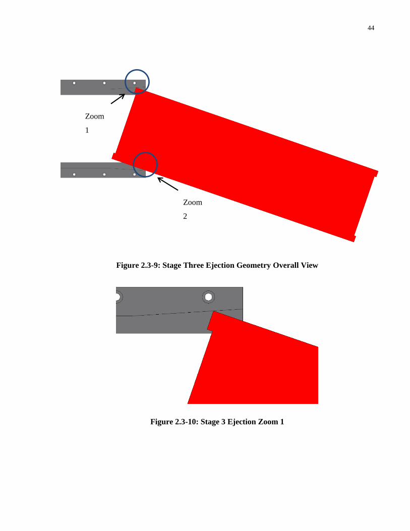
44
Figure 2.3-9: Stage Three Ejection Geometry Overall View
Figure 2.3-10: Stage 3 Ejection Zoom 1
Zoom
1
Zoom
2

45
Figure 2.3-11: Stage 3 Ejection Zoom 2
2.3.2.4 Pusher Plate Contact Geometry
Sections 2.3.2.1 through 2.3.2.3 give rise to three phases of the spacecraft deployment and do
not take the separation even between the spacecraft and pusher plate into account. The separation
event occurs once the XPOD main spring has reached its free length during the deployment,
which causes a pulling force on the pusher plate. Since there are no fasteners or adhesive joining
the spacecraft and pusher plate, theoretically the spacecraft will maintain the velocity that it has
at the instant that the spring reaches its free length, while the pusher plate will experience
acceleration back into the XPOD body. This causes the pusher plate to slow down at the instant
that the main spring free length is reached and separation to occur at that instant. This can occur
during any of the three geometric stages, depending on how the main spring is designed, and
gives rise to the remaining three deployment stages. Figure 2.3-12 shows a deployment that is
constrained to limiting angles for phases one through three, with the pusher plate separation
shown as well:
a)
b)
c)
d)

46
e)
f)
g)
h)
i)
j)
Figure 2.3-12: XPOD Deployment Steps with Pusher Plate
In image a) the deployment begins, the pusher plate and spacecraft are still in contact, and the
geometry is that of phase one. The deployment continues through image b), until image c) where
the pusher plate and spacecraft are no longer in contact. The spacecraft continues to travel out of
the XPOD, not in contact with the pusher plate from image d) to image e). Stage two geometry
begins in image f) and continues until image g). Stage three geometry beings in image h) and is
continued until the spacecraft is leaving the XPOD in image j).
The deployment illustrated in Figure 2.3-12 was based primarily on the geometry of a 3U (See
[16]) spacecraft with increased taper angles and clearance between the rails to make the
spacecraft tipping angles more noticeable. This geometric scenario resulted in the separation
event occurring during phase 1 of the rail geometry as described in Section 2.3.2. However, since
this event can occur during any one of the phases, the analysis includes a pusher plate separation
check at all stages of the deployment to correctly calculate the geometric constraints.
It should be noted that Figure 2.3-12 does not include the solid model of the XPOD main spring
since it is not needed to show the separation and deployment events. Also, Figure 2.3-12 does
not show how the pusher plate will be pulled back into the XPOD due to the pulling force of the
XPOD main spring once the separation has occurred. This was not shown because the particular

47
dynamics of that event do not affect how the spacecraft tipping angle is constrained by the rails
after separation since the pusher plate and spacecraft are not in contact.
2.3.2.5 Variable Definitions
Figure 2.3-13 and Figure 2.3-15 are illustrations of the geometric variables that are described in
Table 3. It should be noted that the reference frames used in these images do not correspond
with those of the XPOD or spacecraft. The references frames that are used are solely used for
this solution.
Figure 2.3-13: Spacecraft in Armed Configuration in Y-P Plane
Figure 2.3-13 gives variable definitions based on spacecraft rotation about the X-Axis. To
determine the variable definitions for rotation about the Y-Axis, the variables in Figure 2.3-14
would be used. They are all the same, except for the center of mass offset (𝑐𝑚).

48
Figure 2.3-14: Spacecraft in Armed Configuration in X-P Plane
Figure 2.3-15 shows a zoomed in view of the taper in the launch rail detailing the variables used
to define the length of the taper, and the taper height:
Figure 2.3-15: XPOD Launch Rail Taper Geometry

49
Table 3 defines the input variables to the tip off rate solution along with a brief description of
each variable:
Table 3: List of Input Variables Used in Calculations and MATLAB Code
Variable Name Description
𝑷 Solution “position” coordinate direction
𝑷𝒕𝒂𝒑𝒆𝒓 Position that the rail taper begins in
𝑭𝒔𝒑𝒓𝒊𝒏𝒈 Force exerted on the pusher plate by the XPOD main spring
𝒉𝒕𝒂𝒑𝒆𝒓 XPOD rail taper height
𝒍𝒕𝒂𝒑𝒆𝒓 XPOD rail taper length
𝜽𝒕𝒂𝒑𝒆𝒓 The taper angle of the XPOD rail tapers
𝒉𝒊𝒏𝒔𝒊𝒅𝒆 XPOD rail to rail height
𝒉𝒑𝒑 The dimension of the pusher plate between XPOD rails
𝒍𝒑𝒑 Length of pusher plate in deployment direction
𝒍𝒔𝒂𝒕 Length of satellite in the deployment direction
𝒉𝒔𝒂𝒕 Dimension of satellite between XPOD rails
𝒄𝒎𝒙 Offset of satellite center of mass in the solution X direction
𝒄𝒎𝒚 Offset of satellite center of mass in the solution Y direction

50
2.3.3 Relevant Equations
The following equations were used in calculating the tip-off rates when a spacecraft is ejected
from an XPOD. Some of the equations have variables that change as the spacecraft is ejected,
which are calculated at different steps/iterations.
2.3.3.1 Linear Ejection Profile Equations
The effective spring constant of the pusher plate preloads is found using the following (See
Section 2.2.1 for more information):
𝑘𝑝𝑟𝑒 =
𝐹𝑝𝑟𝑒𝑚𝑎𝑥 − 𝐹𝑝𝑟𝑒𝑚𝑖𝑛
∆𝑃𝑝𝑟𝑒
(2.34)
where
𝑘𝑝𝑟𝑒 is the effective spring constant for the pusher plate preload stacks
𝐹𝑝𝑟𝑒𝑚𝑎𝑥 is the force that the preload typically exerts when the XPOD is armed
𝐹𝑝𝑟𝑒𝑚𝑖𝑛 is the force that the preload typically exerts when the XPOD is unarmed
∆𝑃𝑝𝑟𝑒 is the typical deflection of the pusher plate preload
The compression of the pusher plate preloads when the XPOD is unarmed is found using the
following:
𝑃𝑝𝑟𝑒1
=𝐹𝑝𝑟𝑒
𝑘𝑝𝑟𝑒
(2.35)
where
𝑃𝑝𝑟𝑒1 is the compression of the preload stack when in its unarmed state
The compression of the pusher plate preloads when the XPOD is armed is found using the
following:
𝑃𝑝𝑟𝑒2= 𝑃𝑝𝑟𝑒1
+ ∆𝑃𝑝𝑟𝑒 (2.36)

51
where
𝑃𝑝𝑟𝑒2 is the compression of the preload stack in its armed position
The velocity that the spacecraft and pusher plate will have as result of the energy contained in
the pusher plate preloads is found using the following and assuming no losses:
𝑣𝑝𝑟𝑒 = √𝑘𝑝𝑟𝑒(𝑃𝑝𝑟𝑒2
2 − 𝑃𝑝𝑟𝑒12 )
𝑚𝑡
(2.37)
where
𝑚𝑡 = 𝑚𝑝𝑝 + 𝑚𝑠𝑎𝑡
and
𝑣𝑝𝑟𝑒 is the velocity that will result for the pusher plate and spacecraft from the
preload stack energy
𝑚𝑡 is the combined mass of the spacecraft and pusher plate
𝑚𝑝𝑝 is the mass of the XPOD pusher plate
𝑚𝑠𝑎𝑡 is the mass of the satellite being ejected
The main spring force (𝐹𝑠𝑝𝑟𝑖𝑛𝑔𝑖) that acts on the pusher plate can be found using Equation (2.38)
when the pusher plate and spacecraft are still in contact.
𝐹𝑠𝑝𝑟𝑖𝑛𝑔𝑖= 𝑘𝑠𝑝𝑟𝑖𝑛𝑔 (𝑙𝑠𝑝𝑟𝑖𝑛𝑔𝑓
− 𝑙𝑠𝑝𝑟𝑖𝑛𝑔𝑐− 𝑃𝑖) (2.38)
where
𝑘𝑠𝑝𝑟𝑖𝑛𝑔 is the spring constant of the XPOD main spring
𝑙𝑠𝑝𝑟𝑖𝑛𝑔𝑓 is the free length of the XPOD main spring
𝑙𝑠𝑝𝑟𝑖𝑛𝑔𝑐 is the length of the XPOD main spring when it is armed
𝑃𝑖 is the position of the spacecraft at iteration “i”

52
The time between the positions of two consecutive iterations is found using Equation (2.39). This
duration of time can also be thought of as the time it takes to pass through an iteration.
∆𝑡𝑖 =
∆𝑃
𝑣𝑖 (2.39)
where
∆𝑡𝑖 is the time it takes to pass through the current iteration
∆𝑃 is the distance between the positions of two consecutive iterations. This is
deemed the position stepping size and is held constant.
𝑣𝑖 is the spacecraft linear velocity during the current iteration
The time that it has taken for the spacecraft to reach the current solution iteration can be then be
found using:
𝑡𝑖 = 𝑡𝑖−1 + ∆𝑡𝑖−1 (2.40)
where
𝑡𝑖 is the time that it has taken the spacecraft reach the current iteration
𝑡𝑖−1 is the time that it took the spacecraft to reach the previous iteration
∆𝑡𝑖−1 is the time it took the spacecraft to pass through the previous iteration
Finally, the linear velocity of the spacecraft can be determined using:
𝑣𝑖 = 𝑣𝑖−1 +
𝐹𝑠𝑝𝑟𝑖𝑛𝑔𝑖−1
𝑚𝑡∆𝑡𝑖−1 (2.41)
where
𝑣𝑖−1 is the velocity at the previous iteration
𝐹𝑠𝑝𝑟𝑖𝑛𝑔𝑖−1 is the main spring force acting on the pusher plate during the previous
iteration
∆𝑡𝑖−1 is the time it took the spacecraft to pass through the previous iteration
53
2.3.3.2 Geometric Constraint Equations
The limiting angles that the XPOD rails constrain the rotating assembly to must also be
calculated. The taper angle of the XPOD rails is found using:
𝜃𝑡𝑎𝑝𝑒𝑟 = tan−1 (
ℎ𝑡𝑎𝑝𝑒𝑟
𝑙𝑡𝑎𝑝𝑒𝑟)
(2.42)
The distance between the point where the spacecraft assembly touches the top rail and where the
spacecraft assembly touches the bottom rail, measured in the axis perpendicular to the
deployment axis, is required in the solution. This value, which will hereon be referred to as the
“total height”, will change as the spacecraft is ejected and must be calculated at every position.
When constrained to phase one geometry, the relationship is given by:
𝐻𝑡𝑖= ℎ𝑖𝑛𝑠𝑖𝑑𝑒 (2.43)
where
𝐻𝑡𝑖 is the total height at position “i”
When the spacecraft assembly passes into the phase two constraint scenario, the total height is
calculated using:
𝐻𝑡𝑖= ℎ𝑖𝑛𝑠𝑖𝑑𝑒 + ℎ𝑡𝑎𝑝𝑒𝑟 (2.44)
Once the spacecraft assembly has passed into the phase three constraints scenario, the total
height is given by:
𝐻𝑡𝑖= ℎ𝑖𝑛𝑠𝑖𝑑𝑒 + ℎ𝑡𝑎𝑝𝑒𝑟 + ℎ𝑝𝑖
(2.45)
where
ℎ𝑝𝑖 is the partial height added by the top rail taper at position “i”
The partial height arises from the top spacecraft corner dragging along the taper on the top rail.
As the corner drags along the taper, height is added that ranges from no additional height at the

54
leading edge of the taper, to a height equal to the taper height (ℎ𝑡𝑎𝑝𝑒𝑟) when the spacecraft is at
its last position inside the XPOD.
The equation used to calculate the amount of partial height that exists depending on the current
position of the spacecraft is:
ℎ𝑝𝑖= (𝑃𝑖 − 𝑃𝑡𝑎𝑝𝑒𝑟)tan (𝜃𝑡𝑎𝑝𝑒𝑟)
(2.46)
Now, the limiting angle for the spacecraft can be found as a function of its position. When the
spacecraft is in the first phase of its deployment, Equation (2.47) should be used. When the
spacecraft is in phase two or three of its deployment, then Equation (2.48) should be used. (See
[17] for derivation)
0 = ℎ𝑠𝑎𝑡 cos 𝜃𝑔𝑒𝑜𝑖+ (ℎ𝑠𝑎𝑡 sin 𝜃𝑔𝑒𝑜𝑖
+ 𝑙𝑝𝑝 cos 𝜃𝑔𝑒𝑜𝑖+ 𝑃𝑡𝑎𝑝𝑒𝑟 − 𝑃𝑖) tan 𝜃𝑔𝑒𝑜𝑖
− 𝐻𝑡𝑖
(2.47)
0 = ℎ𝑠𝑎𝑡 cos 𝜃𝑔𝑒𝑜𝑖+ (ℎ𝑠𝑎𝑡 sin 𝜃𝑔𝑒𝑜𝑖
+ 𝑙𝑝𝑝 cos 𝜃𝑔𝑒𝑜𝑖+ 𝑙𝑠𝑎𝑡 − 𝑃𝑖) tan 𝜃𝑔𝑒𝑜𝑖
− 𝐻𝑡𝑖 (2.48)
where
𝜃𝑔𝑒𝑜𝑖 is the limiting angle at position “i”
These equations would typically be solved using MATLAB where all variables are known
except for 𝜃𝑔𝑒𝑜𝑖.
Determination of the angular velocity that would result if the spacecraft followed the limiting

55
angles between two iterations (a.k.a. the “geometric angular velocity”) can then be found using:
𝜔𝑔𝑒𝑜𝑖
=𝜃𝑔𝑒𝑜𝑖
− 𝜃𝑔𝑒𝑜𝑖−1
∆𝑡𝑖−1
(2.49)
where
𝜔𝑔𝑒𝑜𝑖 is the geometric angular velocity
𝜃𝑔𝑒𝑜𝑖−1 is the limiting angle for the assembly at the previous iteration
Once the geometric angular velocity has been found, all of the information available from purely
geometric constraints has been found. Now, the consideration of the forces acting on the
spacecraft can begin such that physically relevant rotation angles and rates can be found.
2.3.3.3 Ejection Analysis Considering Forcing
Up to now the presented equations used to determine rotation angles only took the geometric
boundary conditions into account. These boundaries, while still giving important information
since the spacecraft will be constrained within the boundary angular limits may not be realistic.
This is because the forces required to have the spacecraft follow these boundaries may be much
higher than the actual rotation inducing forces that are experienced based on the assumptions
given in Section 2.3.1. The following equations are then used to calculate the spacecraft rotation
profile as a function of both the boundary conditions and rotation inducing forces.
The sum of torques acting on the block during the current iteration, assuming no impact occurs
between the block and the rails, is found using:
∑𝜏𝑖 = 𝐹𝑠𝑝𝑟𝑖𝑛𝑔𝑖𝑐𝑚 (2.50)
where
∑𝜏𝑖 is the sum of torques acting on the block
The axis in which the torques are acting about will depend on the plane that the solution is being
found in. For example, if the solution is being found in the X-P plane, then the torques will be

56
about the Y-Axis, and the center of mass offset between the P-Axis and the main spring force
will be 𝑐𝑚𝑦. On the other hand, if the solution is being found in the Y-P plane, then the torques
will be about the X-Axis, and the center of mass offset between the P-Axis and the main spring
force will be 𝑐𝑚𝑥.
Using the sum of torques found in Equation (2.50), the current block angular velocity is found
using:
𝜔𝑖 =
∑𝜏𝑖−1 ∆𝑡𝑖−1
𝐼+ 𝜔𝑖−1 (2.51)
where
𝜔𝑖 is the block actual angular velocity in the current iteration
𝜔𝑖−1 is the block actual angular velocity in the previous iteration
∑𝜏𝑖−1 is the sum of torques acting on the block over the previous iteration
𝐼 is the moment of inertia of the block
The axis of rotation for the spacecraft in this equation will correspond to the axis that the
moment of inertia is calculated from, along with the axis about which the torques are calculated.
The moment of inertia must also be that of the spacecraft and pusher plate assembly, if they are
still in contact, since they are assumed to rotate together.
The actual angle that the block has rotated to is found using:
𝜃𝑖 = 𝜃𝑖−1 + 𝜔𝑖−1∆𝑡𝑖−1 (2.52)
where
𝜃𝑖 is the actual angle that the block is at, at the current iteration
𝜃𝑖−1 is the actual angle that the block was at, at the previous iteration
If the angle that the spacecraft has rotated to is greater than the allowable geometric angular limit
(ie 𝜃𝑖 > 𝜃𝑔𝑒𝑜𝑖) then impact has occurred between the block and rail. The current angle must then
be set to the allowable geometric angle (ie 𝜃𝑖 = 𝜃𝑔𝑒𝑜𝑖) and the effective angular velocity over the
previous time step must be recalculated using Equation (2.53), which is a modified version of

57
Equation (2.52):
𝜔𝑛𝑒𝑤𝑖−1
=𝜃𝑖 − 𝜃𝑖−1
∆𝑡𝑖−1
(2.53)
where
𝜔𝑛𝑒𝑤𝑖−1 is the effective angular velocity during the previous iteration
The acceleration that the block experienced as a result of the impact between the block and the
rails is found using:
𝛼𝑖−1 =
𝜔𝑛𝑒𝑤𝑖−1− 𝜔𝑖−1
∆𝑡𝑖−1
(2.54)
where
𝛼𝑖−1 is the angular acceleration during the previous iteration and will be negative
Equation (2.54) uses values that are all taken from a previous iteration (ie. 𝑖 − 1) because the
angular velocity at the current iteration must have already been found to determine if impact
occurred. Therefore, as part of the calculation process of the current iteration, you may still need
to find results that occur at the previous iteration’s position.
Since an acceleration occurred during the previous iteration, the torque that was originally found
for that iteration using Equation (2.50), which assumed that no impact occurred, is no longer
correct. The sum of torques that acted during the previous iteration can now be found using:
∑𝜏𝑛𝑒𝑤𝑖−1= 𝐹𝑠𝑝𝑟𝑖𝑛𝑔𝑖−1
𝑐𝑚 + 𝐼𝛼𝑖−1 (2.55)
where
∑𝜏𝑛𝑒𝑤𝑖−1 is the corrected sum of torques that acted during the previous
iteration

58
2.3.4 Implementation of the Solution Method
This section will detail the implementation of the solution method used in predicting the tip off
rates of spacecraft that are deployed from XPODs. For iterative sections a single iteration will be
shown, but the iteration method will still be described.
2.3.4.1 Set XPOD Dependent Variables
The first step in solving for the tip off rate is to determine all of the following variables, which
are determined by direct measurement, that are associated with the XPOD being used:
1. ℎ𝑡𝑎𝑝𝑒𝑟 2. 𝑙𝑠𝑝𝑟𝑖𝑛𝑔𝑓
3. 𝐹𝑝𝑟𝑒𝑚𝑖𝑛 4. 𝑚𝑝𝑝
5. 𝑙𝑡𝑎𝑝𝑒𝑟 6. 𝑙𝑠𝑝𝑟𝑖𝑛𝑔𝑐
7. ℎ𝑖𝑛𝑠𝑖𝑑𝑒 8. 𝑥𝑝𝑟𝑒
9. 𝑙𝑝𝑝 10. 𝐹𝑝𝑟𝑒𝑚𝑎𝑥
11. 𝑘𝑠𝑝𝑟𝑖𝑛𝑔
2.3.4.2 Set Spacecraft Dependent Variables
The second step is to determine all of the following variables, which are determined by direct
measurement, that are associated with the spacecraft being ejected:
1. 𝑙𝑠𝑎𝑡 2. 𝑚𝑦
3. 𝑚𝑠𝑎𝑡 4. 𝑐𝑚𝑥
5. ℎ𝑠𝑎𝑡 6. 𝐼𝑥𝑥
7. 𝐼𝑦𝑦
59
2.3.4.3 Set Iteration Stepping Distance and Calculate Preliminary Values
Following the determination of all of the properties that are used in the solution, which are
derived from XPOD geometry, spacecraft geometry, and spacecraft physical properties, the
following initial values can be obtained.
The position step size, which is a selected value and determines the linear position separation
between iterations in the P-axis:
∆𝑃
The coordinate, in the P-axis, of the pusher plate to spacecraft interface once the XPOD main
spring has reached its free length:
𝑃𝑠𝑝𝑟𝑖𝑛𝑔 = 𝑙𝑠𝑝𝑟𝑖𝑛𝑔𝑓− 𝑙𝑠𝑝𝑟𝑖𝑛𝑔𝑐
(2.56)
The maximum position allowable in the solution coordinate system:
𝑃𝑚𝑎𝑥 = 𝑙𝑠𝑎𝑡 (2.57)
The coordinate, in the P-axis, of the leading edge of the XPOD rail taper:
𝑃𝑡𝑎𝑝𝑒𝑟 = 𝑃𝑚𝑎𝑥 − 𝑙𝑡𝑎𝑝𝑒𝑟
(2.58)
The total mass of the spacecraft and pusher plate:
𝑚𝑡 = 𝑚𝑝𝑝 + 𝑚𝑠𝑎𝑡 (2.59)
After the determination of the above constant values, the XPOD rail taper angle can be found
using Equation (2.42). Then the pusher plate preload spring constant (𝑘𝑝𝑟𝑒), initial compression
(𝑃𝑝𝑟𝑒1), armed compression (𝑃𝑝𝑟𝑒2
) can be found using Equations (2.34), (2.35), and (2.36)
respectively. Finally, the resulting velocity that the pusher plate preload imparts on the spacecraft
and pusher plate (𝑣𝑝𝑟𝑒) can be found using Equation (2.37).

60
2.3.4.4 Calculation of the Linear Ejection Velocity Profile
The calculation of the linear ejection velocity profile can now be completed, which neglects
frictional effects and energy loss in other areas. This assumption is made such that the ejection
velocity is as high as possible. This will result in the shortest time differences between iterations,
and therefore between angular positions, which should give higher angular velocities. Therefore,
since higher spacecraft tumble rates are of more concern when considering recovery to a stable
attitude, this should also yield a more conservative analysis.
2.3.4.4.1 Set and Calculate Initial Conditions
The following initial conditions for the block can be set and calculated, starting with the starting
time for the solution (a.k.a. the time at iteration zero):
𝑡0 = 0 𝑠
The velocity at iteration zero, which is equal to the velocity that the pusher plate preloads impart
onto the block, can also be set:
𝑣0 = 𝑣𝑝𝑟𝑒
The spring force acting during iteration zero (𝐹𝑠𝑝𝑟𝑖𝑛𝑔0) is found using Equation (2.38) and the
time it takes to pass through iteration zero (∆𝑡0) is found using Equation (2.39).
2.3.4.4.2 Calculate the Ejection Profile for Remaining Positions
While the spacecraft is still inside the XPOD (i.e. 𝑃𝑖 < 𝑃𝑚𝑎𝑥), the following iterative section
should be repeated such that the linear ejection profile of the spacecraft is determined:
First, calculate the time (𝑡𝑖) at the start of the current iteration using Equation (2.39). Then,
calculate the linear velocity (𝑣𝑖) that the block is travelling at during the current iteration using
Equation (2.41). Next, if the XPOD main spring has not reached its free length (i.e. 𝑃𝑖 <
𝑃𝑠𝑝𝑟𝑖𝑛𝑔), then calculate the main spring force (𝐹𝑠𝑝𝑟𝑖𝑛𝑔𝑖) using Equation (2.38). If the main spring
has reached its free length(𝑖. 𝑒. 𝑃𝑖 ≥ 𝑃𝑠𝑝𝑟𝑖𝑛𝑔), then set the main spring force to zero. Finally,
using the current iterations velocity, along with the position step size that was chosen at the

61
beginning of the solution, find the time it takes to pass through the iteration (∆𝑡𝑖) using Equation
(2.39).
Once all iterations have completed, a list of times, velocities, and spring forces as a function of
position will be generated. These values will be used in the remaining sections of the solution.
2.3.4.5 Calculate the Limiting Spacecraft Angles as a Function of Position
Here the limiting angular positions that satisfy the geometric constraints shown in Section 2.3.2
are calculated. Forcing is not considered at this point since this is only a geometric consideration.
The results of this section can then be used to check for impact and sliding when the torques on
the block are considered in Section 2.3.4.6.
The calculation begins at iteration zero with the block under stage one geometric constraints.
First, the total internal height (𝐻𝑡𝑖) must be found using Equation (2.43). Then, a determination
must be made as to if the pusher plate and spacecraft are still in contact. If they are in contact
(i.e. 𝑃𝑖 < 𝑃𝑠𝑝𝑟𝑖𝑛𝑔) then the length of the pusher plate (𝑙𝑝𝑝) must be included when solving for the
limiting angle (𝜃𝑔𝑒𝑜𝑖), and if they are not (i.e. 𝑃𝑖 ≥ 𝑃𝑠𝑝𝑟𝑖𝑛𝑔), then it can be ignored. The limiting
angle can now be calculated using Equation (2.47). These phase one limiting angle calculations
should be repeated while the phase one geometric conditions are met (i.e. 𝜃𝑖 < 𝜃𝑡𝑎𝑝𝑒𝑟 and 𝑃𝑖 <
𝑃𝑡𝑎𝑝𝑒𝑟).
Next, once the block has passed into phase two geometry the calculation begins with finding the
total internal height using Equation (2.44). Then the same pusher plate contact rules as in the
phase one scenario are applied, such that the pusher plate length will only be included in
calculating the limiting angle if it and the spacecraft are still in contact. Then the limiting angle
can be calculated using Equation (2.48). This process should be repeated while phase two
geometric conditions are met (i.e. 𝑃𝑖 < 𝑃𝑡𝑎𝑝𝑒𝑟).
The block is now subject to phase three geometry. First, the partial height (ℎ𝑝𝑖) must be
calculated for the given iteration using Equation (2.46). The partial height can then be used in
finding the total internal height using Equation (2.45). The same pusher plate contact rules as in
the phase one and two scenarios are applied , such that the pusher plate length will only be
62
included in calculating the limiting angle if it and the spacecraft are still in contact. Then the
limiting angle can be calculated using Equation (2.48). This process should be repeated while for
the remaining positions (i.e. 𝑃𝑖 < 𝑃𝑚𝑎𝑥).
Now that the limiting angles have been calculated at all positions of interest, the geometric
angular velocity (𝜔𝑔𝑒𝑜𝑖) for each position can be found using Equation (2.49).
2.3.4.6 Calculate the Spacecraft Tipping Profile
This section of the analysis calculates the angle and angular velocity of the spacecraft that is due
to the torque generated by the offset between the spring force and the spacecraft center of mass.
It also takes the rail geometry into account such that impacts between the rails and rotating body
constrain the rotation of the spacecraft.
This analysis assumes the spacecraft has no initial angular velocity or displacement. It also
assumes planar motion of the spacecraft for the solution, and that the angular displacements are
small. Therefore, to find the overall magnitude of the angular velocity of the spacecraft, two
orthogonal angular velocities are first calculated. The resulting magnitude is then found from the
RSS value of the two results.
First, set the initial conditions of the spacecraft and calculate the initial torque acting on the
spacecraft (∑𝜏0) using Equation (2.50). These are the only values required for the first iteration.
𝜃0 = 0
𝜔0 = 0 [1
𝑠𝑒𝑐]
Now, the next iteration may begin, and there are two scenarios for each new iteration. The first is
when no impact occurs between the block and the XPOD rails, and the second is when impact
does occur. When impact occurs the angle that the spacecraft has rotated to at the current
position (i.e. 𝜃𝑖), as a result of the angular velocity from the previous iteration,
exceeds the limiting angle for the current position (i.e. 𝜃𝑖 > 𝜃𝑔𝑒𝑜𝑖). Therefore, each new iteration
must begin with calculating the angle that the block has rotated to as a result of the previous
iterations angular velocity using Equation (2.52), followed by checking if this angle causes

63
impact. Then, depending on if impact did or did not occur, a slightly different process is carried
out. Both processes will be given in what follows.
Assuming that impact has occurred, the current angle must be set to the limiting angle for the
current position (i.e. 𝜃𝑖 = 𝜃𝑔𝑒𝑜𝑖) and the angular velocity for the previous iteration must be
updated to the result of Equation (2.53) (i.e. 𝜔𝑛𝑒𝑤𝑖−1). The angular acceleration that acted during
the previous iteration as a result of the impact (𝛼𝑖−1) is found then using Equation (2.54). The
sum of torques that acted during the previous iteration (∑𝜏𝑛𝑒𝑤𝑖−1) can now be found using
Equation (2.55), which is used to update the original sum of torques acting on the block during
the previous iteration. Now, the current angular velocity (𝜔𝑖) is found using Equation (2.51) and
the torques acting on the block in the current iteration are found using Equation (2.50).
Assuming that impact has not occurred, the angular displacement of the block at the current
position is kept as the result of Equation (2.52). Then, the current angular velocity is found using
Equation (2.51), and the torques acting on the block in the current iteration are found using
Equation (2.50).
After solving for the block angle and angular velocity at each position, then the solution is
complete. This process must be completed for both the X-P plane and the Y-P plane. The results
can then be combined to give the magnitude of the angular velocities for each iteration using:
𝜔𝑚𝑎𝑔𝑖
= √𝜔𝑥𝑖2 + 𝜔𝑦𝑖
2 (2.60)
The magnitude of the angular velocity at the final iteration, which is when 𝑃𝑖 = 𝑃𝑚𝑎𝑥 , is deemed
to be the tip-off rate for the spacecraft. The results of three different spacecraft solutions will be
given in Section 2.3.5.
2.3.5 Tip-Off Rate Analysis Results
Originally, this tip off rate analysis was created to determine the expected tip off rate for the
CanX-7 satellite. However, since CanX-7 has not flow there is no true way to verify if this

64
method produces valid results for that mission. On the other hand, the CanX-2 mission has
flown, was ejected from the same XPOD type that CanX-7 will be ejected from, and has the
same form factor as CanX-7. Therefore, for verification of the 3U form factor version of this
solution, the data from CanX-2 was used for comparison.
On the other hand, although not the original motivation for this work, this analysis was run for
both the AISSat-1 and UNIBRITE busses. These busses have both already been flown, have
measured bus properties, and have on-orbit sensor data for their initial angular rates. Therefore,
the true verification of this method was completed by comparing the analysis results with the
sensor data for these two missions. The results of these comparisons along with the comparison
between the CanX-7 analysis and CanX-2 on orbit data are shown in Table 4:
Table 4: Summary of Tip-Off Rate Analysis Verification
Spacecraft Predicted Tip Off Rate (𝑑𝑒𝑔𝑟𝑒𝑒
𝑠𝑒𝑐𝑜𝑛𝑑) On-Orbit Tip Off Rate (
𝑑𝑒𝑔𝑟𝑒𝑒
𝑠𝑒𝑐𝑜𝑛𝑑)
CanX-2 CanX-7: 3.96 3-5
AISSat-1 6.13 ~6
UNIBRITE 7.82 8-9
Based on the results summary shown in Table 4, it seems that the solution method produces
predictions within two degrees per second of the tip-off rates measured on orbit. This has
allowed the CanX-7 attitude control system designer to have insight into the expected tipoff rates
for their mission, which was the goal of this analysis. However, these results do not include
quantification of the errors on the input variables. Therefore, future work should be completed
for the algorithm to determine error bounds for the results by quantifying the input errors.

65
2.4 EV9 Mechanical Design
This section details the changes that took place from the original EV9-A mission to the current,
EV9, mission. These changes were carried out because of the new contractual agreements that
changed the scope of the mission. Originally, EV9-A did not have 3-axis attitude control, and
had requirements from the launch provider that resulted in the use of all deployable appendages
instead of fixed appendages. The EV9 mission now has a requirement for 3-axis attitude control,
along with relaxed launch vehicle requirements which allow for the use of fixed UHF antennas.
There is also a different payload in the EV9 mission when compared to the original EV9-A
mission.
2.4.1 EV9-A vs. EV9 vs AISSat-2 Comparison
The following table gives a comparison between the components that are part of the EV9-A,
EV9 and AISSat-2 busses:
Table 5: Bus Subsystems Summary
System Name EV9-A EV9 AISSat-2
AISSat Payload Yes No Yes
NTS-Payload Yes No No
EV9 Payload No Yes No
Deployable VHF Antenna Yes Yes No
Deployable UHF Antennas (4) Yes No No
Power Board Yes Yes Yes
Battery Packs (2) Yes Yes Yes
House Keeping Computer Yes Yes Yes
Attitude Control Computer Yes Yes Yes
Payload Computer No No Yes

66
VHF Antenna Switch Yes No No
Hysteresis Rods Yes No No
S-Band Patch Antennas (2) Yes Yes Yes
Sun Sensors (6) No Yes Yes
Magnetometer No Yes Yes
GPS Antenna No No Yes
GPS Radio No No Yes
UHF Radio Yes Yes Yes
S-Band Radio Yes Yes Yes
Rate Sensor No Yes Yes
Reaction Wheels (3) No Yes Yes
Magnetorquers (3) No Yes Yes
Many of the changes from EV9-A to EV9 are a result of the addition of a 3-axis attitude control
system and removal of the secondary payload. The differences compared to AISSat-2 are mostly
a consequence of launch vehicle volume restrictions and not requiring GPS antennas.
2.4.2 EV9 Mechanical Design Requirements
The following list of requirements was generated for the design of the EV9 bus:
1) The VHF antenna load bracket from EV9-A shall be used for the VHF antenna in EV9.
2) Compatibility of the bus with both SFL deployable and fixed UHF antennas shall be
maintained.
67
3) The EV9 design shall be based upon the AISSat-2 design when similar components are
used.
4) The spacecraft shall be oriented in its XPOD with the deployable VHF antenna being
held down by the XPOD door.
5) Compatibility for both an internal and external magnetometer shall be maintained.
The requirements above were used to make the changes from the original EV9-A structure to the
modified version that was required for EV9. There were other requirements that were followed
in the design of the original GNB, but they were not necessarily specific to the EV9 mission so
they were not repeated in the list above. More information on GNB requirements can be found in
[18].
2.4.3 Design Process
The starting point for the EV9 structure was the previously existing EV9-A solid model. From
this solid model, a separate version was created that could be used for modelling the structure
that would be used for EV9. The modifications that were made are detailed in the following lists
and images:
+Z Tray:
A rate sensor was added because the attitude control system for EV9 required a rate sensor,
while the attitude control system for EV9-A did not. The mounting features for the rate sensor
were already part of the EV9-A design since the tray’s design was from a more general GNB
tray design. The added rate sensor can be seen in Figure 2.4-1.

68
Figure 2.4-1: +Z Tray Comparison
-Z Tray:
The mounting holes for the Z-Axis reaction wheel were modified in the EV9 design when
compared to a typical GNB. This was done because the Z-Axis reaction wheel had to be shifted
in the –Z direction by four millimeters such that clearance for the screw heads for the VHF
antenna mounting bracket screws could be made. The Z-Axis wheel was stood off from the –Z
Tray by spacers, and the reaction wheel mounting holes that were in the Y-direction were shifted
in the -Z direction by the required amount. Typically this shifting is not required in the GNB
design because the VHF antenna bracket usually has through holes, and the –Z tray has threaded
holes in an extended boss for their mating. However, since the original EV9-A VHF bracket had
threaded holes for this connection, and not the –Z-tray, the screws heads had to remain inside the
–Z tray, and force the movement of the Z-Axis reaction wheel. Figure 2.4-2 shows a comparison
between the hole locations for the EV9-A structure and the EV9 structure.

69
Figure 2.4-2: -Z Tray Reaction Wheel Hole Relocation
After the holes were moved, the three reactions wheels could be added. These wheels were not
part of the EV9-A design since they were not required for the original attitude control system,
but the modified attitude control did require the wheels. These added reaction wheels are shown
in Figure 2.4-3
The EV9-A structure also had a VHF antenna switch, which was removed in the updated design.
Unlike how the EV9-A mission had two separate payloads that were supposed to use the same
VHF antenna, the EV9 mission only has one payload that requires the use of the VHF antenna.
Therefore, the ability to switch which payload has access to the antenna is no longer required and
the hardware that was designed to implement this capability was removed. The VHF switch
removal is also shown in Figure 2.4-3.

70
Figure 2.4-3: -Z Tray Internal Components Comparison
Sun sensors had to be added to all faces of the satellite because of the updated attitude control
system. The sun sensors that look though both Y Panels are mounted to the –Z Tray and are
shown in Figure 2.4-4 and Figure 2.4-5.
Figure 2.4-4: -Z Tray Sun Sensor Comparison 1

71
Figure 2.4-5: -Z Tray Sun Sensor Comparison 2
+X Panel:
The +X Panel had a Sun sensor added to it, along with a magnetorquer and the magnetorquer
mounting hardware. These components were all added because of the updated attitude control
system and can be seen in Figure 2.4-6 and Figure 2.4-7.
Figure 2.4-6: +X Panel Internal Comparison

72
Figure 2.4-7: +X Panel External Comparison
-X Panel:
The design of EV9-A required hysteresis rods for its attitude control system, but the updated
EV9 design did not require them. A magnetometer was also added to the EV9 design because of
the updated attitude control system. However, when EV9 was being designed the orientation that
the bus would be placed inside the XPOD separation system was unknown, which has impacts
on the placement of the magnetometer. This resulted in multiple mounting locations for the
magnetometer being included in the design of EV9. Therefore, on the –X panel, the hysteresis
rods were removed, a mounting location for the magnetometer was added, and a Sun sensor was
added. These modifications are shown in Figure 2.4-8 and Figure 2.4-9.
Figure 2.4-8: -X Panel Internal Comparison

73
Figure 2.4-9: -X Panel External Comparison
+Y Panel:
The power analysis of the EV9 mission showed that the mission had low power margins. This
necessitated the addition of a solar cell coupon on the +Y face. Another modification on the +Y
Panel was that the VHF antenna guides were moved 90 degrees relative to their original
positions. This was done because in the EV9-A mission the spacecraft was oriented in the XPOD
with its X-Panels on the open faces of the XPOD. This then allowed the deployable VHF
antenna to fold over the –X face. However, because fixed UHF antennas were to be used for
EV9, the Z-Panels had to be on the open sides of the XPOD, which meant the spacecraft had to
rotate 90 degrees. Therefore, the stowed configuration of the VHF antenna had to change such
that the antenna was folded over the –Z face, and therefore facilitated moving the antenna guides
to their new position. A magnetorquer and Sun sensor were also added to the updated +Y Panel.
These changes are all shown in Figure 2.4-10 and Figure 2.4-11.
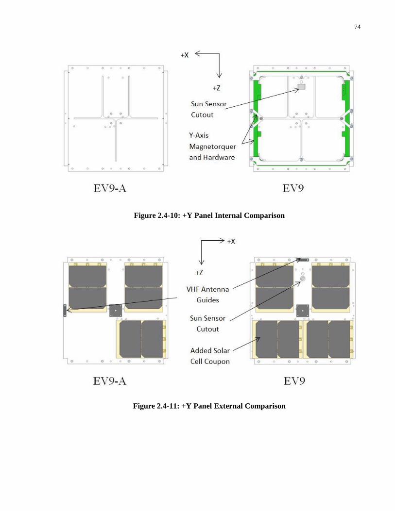
74
Figure 2.4-10: +Y Panel Internal Comparison
Figure 2.4-11: +Y Panel External Comparison

75
-Y Panel:
Similar to the +Y Panel, a Sun senor was added to the –Y Panel and the VHF antenna guides
were shifted 90 degrees. These changes are shown in Figure 2.4-12 and Figure 2.4-13.
Figure 2.4-12: -Y Panel Internal Comparison
Figure 2.4-13: -Y Panel External Comparison

76
+Z Panel:
The EV9-A mission had deployable UHF antennas, which had coaxial cable feed-through
cutouts that were different than the cutouts for fixed style UHF antennas, which were also used
in AISSat-2. Therefore, since it was unknown as to what style of antenna was going to be used
when the EV9 structure was procured, the cutouts were sized to match the larger dimension of
both style of antenna cutout as shown in Figure 2.4-14. A Sun sensor along with internal
magnetometer mounting feautures were also added. These modificaiton are shown in Figure
2.4-15 and Figure 2.4-16. Finally, an external magnetometer boom was added, which was the
primary magnetometer mounting location for EV9. This is shown in Figure 2.4-17.
Figure 2.4-14: UHF Antenna Cutout Comparisons (Dimensions in Millimeters)

77
Figure 2.4-15: +Z Panel Internal Comparison
Figure 2.4-16: +Z Panel External Comparison
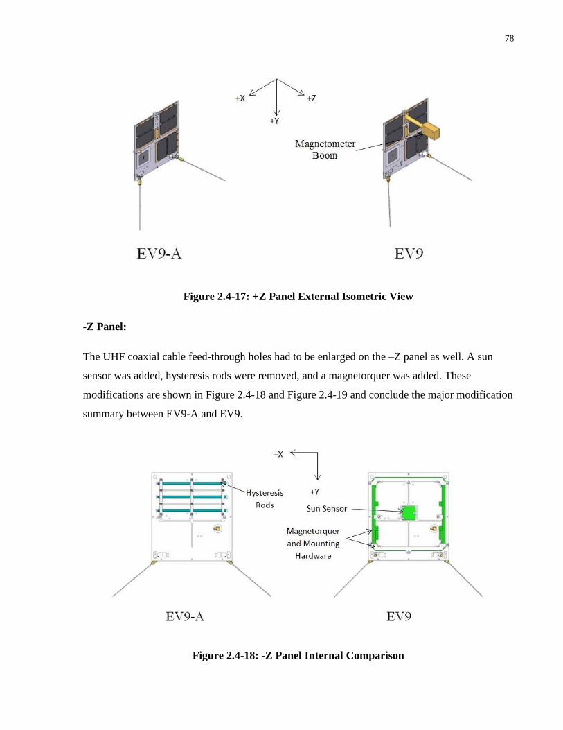
78
Figure 2.4-17: +Z Panel External Isometric View
-Z Panel:
The UHF coaxial cable feed-through holes had to be enlarged on the –Z panel as well. A sun
sensor was added, hysteresis rods were removed, and a magnetorquer was added. These
modifications are shown in Figure 2.4-18 and Figure 2.4-19 and conclude the major modification
summary between EV9-A and EV9.
Figure 2.4-18: -Z Panel Internal Comparison

79
Figure 2.4-19: -Z Panel External Comparison
2.5 NORSAT-1 Mechanical Design
2.5.1 NORSAT-1 Design Requirements and Starting Point
The NORSAT-1 mission mechanical design work began with an existing design of the bus that
was from the proposal stage of the mission. Exterior and interior views of the satellite showing
the proposed layout of components are shown in Figure 2.5-1:
Figure 2.5-1: NORSAT-1 Initial Bus Design
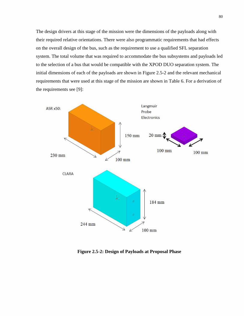
80
The design drivers at this stage of the mission were the dimensions of the payloads along with
their required relative orientations. There were also programmatic requirements that had effects
on the overall design of the bus, such as the requirement to use a qualified SFL separation
system. The total volume that was required to accommodate the bus subsystems and payloads led
to the selection of a bus that would be compatible with the XPOD DUO separation system. The
initial dimensions of each of the payloads are shown in Figure 2.5-2 and the relevant mechanical
requirements that were used at this stage of the mission are shown in Table 6. For a derivation of
the requirements see [9]:
Figure 2.5-2: Design of Payloads at Proposal Phase

81
Table 6: List of NORSAT-1 Relevant Mechanical Requirements
Requirement
Number Requirement Description
1. The spacecraft dimensions, including appendages, should be compatible
with a qualified SFL satellite deployment system.
2. The spacecraft shall include a design feature that can prevent it from
turning on while inside the separation system / launch vehicle.
3. The total launch mass of the spacecraft and its separation system shall be
less than 30 kg.
4. The satellite platform shall accommodate the payloads internally, except
where payload requirements explicitly state otherwise.
5. The CLARA payload shall be accommodated such that its sensor apertures
see the sun during operations.
6. The Langmuir Probes (qty. 4) shall be accommodated externally, parallel to
each other, and orthogonal to the CLARA line of sight.
7.
The AIS antennas (qty. 2) shall be accommodated externally, and be
pointed orthogonal to each other and orthogonal to the Langmuir Probe
booms.
2.5.2 NORSAT-1 Design Iterations
Following the proposal stage of the mission there were updates to the required volumes for both
the CLARA and ASR x50 payloads. The modified dimensions of these two payloads are shown
in Figure 2.5-3 along with their original volumes for comparison:

82
Figure 2.5-3: Modified CLARA and ASR x50 Payload Volumes
The reduced sizes of these payloads allowed for different designs of the bus to be possible since
the payloads were smaller. The first iteration on the design made use of the bus form factor that
would be compatible with the XPOD H27 separation system (See [19]). This design allowed for
an overall volume decrease of the bus and is shown in Figure 2.5-4:
Figure 2.5-4: NORSAT-1 Bus Design, H27 Form Factor

83
Some of the benefits of this design are that the overall volume of the bus is decreased, which
results in lower mass and lower launch cost. However, some of the downfalls of this design are
that there is not much remaining volume in the bus that would allow for the payloads to grow as
the mission progressed, along with the fact that SFL has not yet designed its own structure that is
compatible with the XPOD H27. This would result in more risk in the mission given the
uncertainty of the details of a bus with this form factor, along with the reduced volume margins
in the bus.
While the H27 form factor was being developed, a second option from the proposed bus design
was being looked into. This option was based off the GHGSat-D bus design that was also under
development at SFL. Figure 2.5-5 shows an external and internal view of the GHGSat-D bus
design that was used as the starting point for the second modified option of the NORSAT-1 bus
design:
Figure 2.5-5: Views of GHGSat-D during the NORSAT-1 Preliminary Design Phase [20]
The blue volume that is shown represents the internal payload volume that was available to be
used by the NORSAT-1 mission for payloads. Some of the other modifications that had to be
made were the removal of the star tracker, removal of the UHF antennas, addition of two more
S-Band antennas, and the addition of the exterior solar panel. The design of the NORSAT-1 bus
that resulted from these changes and was the design presented for the Preliminary Design

84
Review for the NORSAT-1 mission is shown in Figure 2.5-6, Figure 2.5-7, Figure 2.5-8, and
Figure 2.5-9:
Figure 2.5-6: NORSAT-1 PDR Bus Design Exterior Views and Rough Dimensions

85
Figure 2.5-7: NORSAT-1 Exterior PDR Design View 1
Figure 2.5-8: NORSAT-1 Exterior PDR Design View 2

86
Figure 2.5-9: NORSAT-1 Interior PDR Bus Design
The external solar panel used in this design was specified to use the same material and supplier
as the external solar panel for the NEMO-AM mission at SFL. There were other design iterations
for the NORSAT mission that attempted to not use an external solar panel, but they resulted in
the bus having faces that would be larger than the PDR version of this design. This then lead to
fairly excessive amounts of extra volume in the bus to exist, which was not beneficial for the
mission due to the extra structure that would be needed. These iterations also left little room on
the solar cell covered panel for thermal tapes, which was anticipated to be an issue from a
thermal standpoint.
Another design choice that was made for the PDR stage of the design was that the CLARA
instrument would be responsible for its own internal thermal control. The CLARA payload,
while taking measurements, requires a maximum temperature drift of 0.1 Celsius per hour for the
sensors in the instrument, which is different than thermal requirements for other SFL satellites.
Typically, the goal of a thermal designer at SFL is to keep all components in a bus within their
survival temperature limits, plus at least a five degree margin, in both a worst case hot and worst
case cold scenario. Therefore, a design that would allow the CLARA payload to have its entire
front face used for the thermal control of its internal sensors, having the sensors thermally
isolated from the bus, and then having the rear portion of the CLARA structure thermally
coupled to the rest of the bus was chosen. This is the reason why the CLARA payload has its

87
front face exposed, and it is not contained within the bus. The details of this design were not
fully finalized at the PDR stage of the mission, but are being worked out as the NORSAT-1
mission continues by the mission’s new mechanical designer.
One final consideration that was made was trying to keep the tips of the Langmuir probe
instruments as far away from the bus as possible. This was required since as the bus goes through
its orbit, it disturbs the plasma that it is travelling through. The probes, which attempt to measure
undisturbed plasma, want to be outside of the volume of plasma that is disturbed by the bus. The
placement that was decided upon was that they come out one of the X-faces since preliminary
mission operation analysis showed this location would result in them typically not being in the
ram or wake direction of the bus in its orbit. They then needed to be as far away from the bus as
possible, and the clearances that were achieved in the design from PDR are shown in Figure
2.5-10:
Figure 2.5-10: Langmuir Probe Clearances from PDR Design

88
There were concerns over the distance between the probe tips and the external solar panel during
the PDR meeting, which then lead to a modified PDR design. This design had both probes
moved toward the +Z panel on both the X panels, and was the final design that was a result of
the thesis work. An image of this design is shown in Figure 2.5-11:
Figure 2.5-11: NORSAT-1 Modified PDR Design

89
Finite Element Modelling
3.1 MiniMags Finite Element Model
The MiniMags mission required a preliminary analysis to determine if the proposed structure for
the bus was a feasible option for the expected payload. To create this model a simplified
approach was used that implemented the use of simplified geometry, lumped masses and face
gluing to reduce the model’s complexity.
Simplified geometry allowed the meshes that were created in the Finite Element Model (FEM) to
neglect small features, which reduced meshing time and reduced simulation time since less
elements were part of the solution. Lumped masses allowed for some of the non-structural
components in the bus to be neglected from a geometric standpoint, and to only consider the
mass and inertia from these components. This also reduced the time it took to create the model
and reduced simulation time. Finally, face gluing is a feature of the NX 8.0 FEM package that
allows individual and dissimilar meshes to be joined together with the use of stiff spring
elements that couple both the rotation and translation of connected elements (See [21]). The
stiffness of the elements that are created is a function of the two meshes being joined together
and will be similar to the average of the two. Using face gluing reduces the amount of time
required to mesh the structure because individual fasteners do not need to be considered,
however it can artificially increase in the overall stiffness of the joint.
All of the above simplification techniques reduce the accuracy of the model, and therefore
caution was used when comparing the results of the analysis against requirements. Higher factors
of safety were used and critical components would need to be modelled with a more
representative model when the design is more mature and less likely to have large changes.
Finally, since the design of the MiniMags bus was very preliminary and could likely experience
fairly large changes if the mission were to continue, a simplified analysis was deemed
appropriate for the feasibility study.

90
3.2 Finite Element Model Setup
Figure 3.2-1 and Figure 3.2-2 show the FEM that was made for the MiniMags structure:
Figure 3.2-1: Overall Top View of FEM
Figure 3.2-2: Overall Bottom View of FEM
3.2.1 Boundary Conditions
Based on the investigation of the launch vehicles from Section 2.1, the following boundary
conditions were derived for use in the finite element model:
1. A 105 g static load applied in any principal axis, not simultaneously. A minimum factor of
safety of 1.41 was considered when reviewing the results to determine feasibility, which was
derived from the shock loading factor of safety requirement of the Ariane 5 launch vehicle
2. A fixed translation and rotation constraint placed on the launch adapter ring, which is shown
in blue in Figure 3.2-3

91
Figure 3.2-3: Bottom View of FEM with Constraints Shown
3.2.2 Modelling Methodology
The FEM that was created for this structural analysis was based on the simplified model of the
spacecraft as previously described. This was done because the purpose of this analysis was to
prove the feasibility of the overall design and not to focus on the fine details associated with the
individual components in the design. The payload, along with other major components such as
the on-board computers, power subsystem, and attitude control system, were modelled as lumped
masses. The overall mass of the modelled spacecraft was made to replicate that of the mass given
by the preliminary mass budget for the spacecraft. This budget was based on the solid model that
was created for MiniMags, along with measured masses of components that were previously
used at SFL.
The FEM was made in the program NX 8.0 using NASTRAN based elements (See [21] for more
information on the following elements that are mentioned). All side panels of the bus were
modeled using 2D-PCOMP elements since they are used for representing honeycomb materials.
The solar cell coupons were modeled using 2D-PCOMP elements as well since they were also a
honeycomb structure. The threaded spacers in these structures were not modeled, but their
masses were accounted for by adding non-structural mass to the applicable structural
components. The adapter ring and plate were modeled using 3D-HEX8 elements. Finally, the
brackets that connect the panels together were modelled using 3D-HEX 8 elements as well.

92
Connections between the solar coupons and the bus were created using rigid RBE-2, 1D
elements, between nodes near the locations of the screws that would be used in the real world.
Connections between the panel joints and panels were created using “face gluing” between the
two interfacing surfaces. Finally, the connections between the adapter ring, adapter plate and bus
were all made using “face gluing” between their interfacing surfaces.
3.2.3 Material Selection
The materials selected for the structural components in the model were derived from the original
solid model of the MiniMags structure. This solid model was generated as part of the earlier
thesis work in the MiniMags feasibility study and was based on the existing NEMO-HD bus.
The physical properties for these materials are given in the table below:
Table 7: Summary of Material Properties Used in the MiniMags FEM
Material Density
(kg/m3)
Eorthogonal
(MPa)
Eparallel
(MPa)
Tensile Yield
Strength (MPa)
Compressive
Yield Strength
(MPa)
Shear
Yield
Strength
(MPa)
5056 Aluminum
Honeycomb Core [22]
97.7 2.03 2030 0.06 5.7 2.1
Aluminum 7075-T6 [23] 2,810 71,700 71,700 503 503 317
Carbon Fiber Reinforced
Plastic [22]
1,800 240,000 240,000 4000 4000 N/A
3.3 Results
After solving the model for the natural frequencies of the bus and for the bus behavior given the
loading described in Section 3.2.1, the following results were obtained.

93
3.3.1 Natural Frequencies
The first natural frequency was determined to be 102Hz and is shown in the image below. The
shape of the mode is a rocking of the bus structure about the Y-axis. In this mode the –Z Panel
does not resonate with the side panels and +Z Panel, and is a partially localized mode since the
entire bus does not resonate as a whole.
Figure 3.3-1: Image of First Natural Frequency
The second natural frequency was determined to be 112Hz and is shown in the image below. The
shape of the mode is a rocking of the entire bus structure about the X-axis. In this mode the –Z
Panel resonates with the side panels and +Z Panel, unlike the first mode, and is not a localized
mode.
Figure 3.3-2: Image of Second Natural Frequency

94
The third natural frequency was determined to be 133Hz and is shown in the image below. The
shape of the mode is a rocking of the entire bus structure about the Y-axis. In this mode the
–Z-Panel resonates with the side panels and +Z Panel, like the second mode, and is again not a
localized mode.
Figure 3.3-3: Image of Third Natural Frequency
3.3.2 Stress Results
The FEM was run using a 105g acceleration in each principal axis, in both the positive and
negative directions, not simultaneously. The worst case stresses were realized when the load was
in the -Z direction. This caused bending of the +Z panel toward the –Z panel, some bulging of
the side panels, and bending of the -Z panel around the separation adapter plate. The image
below shows the resulting displacement plot, where the units are in millimeters:

95
Figure 3.3-4: Overall Nodal Displacement of Bus Components for -Z Loading Case
The following image shows the stresses in the exterior panels from the same loading condition:
Figure 3.3-5: Overall Panel Stress Distribution Image from -Z Loading Case

96
The maximum stress experienced in the panels from this loading case was 135 MPa, which was
found in the skin layer of the –Z panel. A bottom view of this result is shown below:
Figure 3.3-6: Bottom View of -Z Panel Stress Distribution from -Z Loading Case
The maximum stress, and lowest safety factor, in the entire assembly was 171MPa, which was
found in a panel joint that joins the +Z panel and the –X panel. The maximum allowable stress in
this component, with respect to the yield stress is 503 MPa, which results in a factor of safety of
2.94. An image of this is shown below:
Figure 3.3-7: Image of Highest Stress Component from -Z Loading Case

97
3.4 Conclusions
The results of the FEM showed that the feasibility study design of the MiniMags bus met the
stiffness and loading requirements that were derived from the launch vehicle investigation. The
first natural frequency of the bus was found to be 102 Hz, which met the minimum first natural
frequency requirement of 90 Hz. The minimum factor of safety due to the 105g shock load was
found to be 2.94, which met the minimum factor of safety requirement of 1.41. Finally, it should
again be noted that since this modelling effort was at a high level and used coarse meshes along
with simplifications to the structure, that a more detailed analysis should be performed when the
bus design is more mature to ensure that the design requirements are still met.
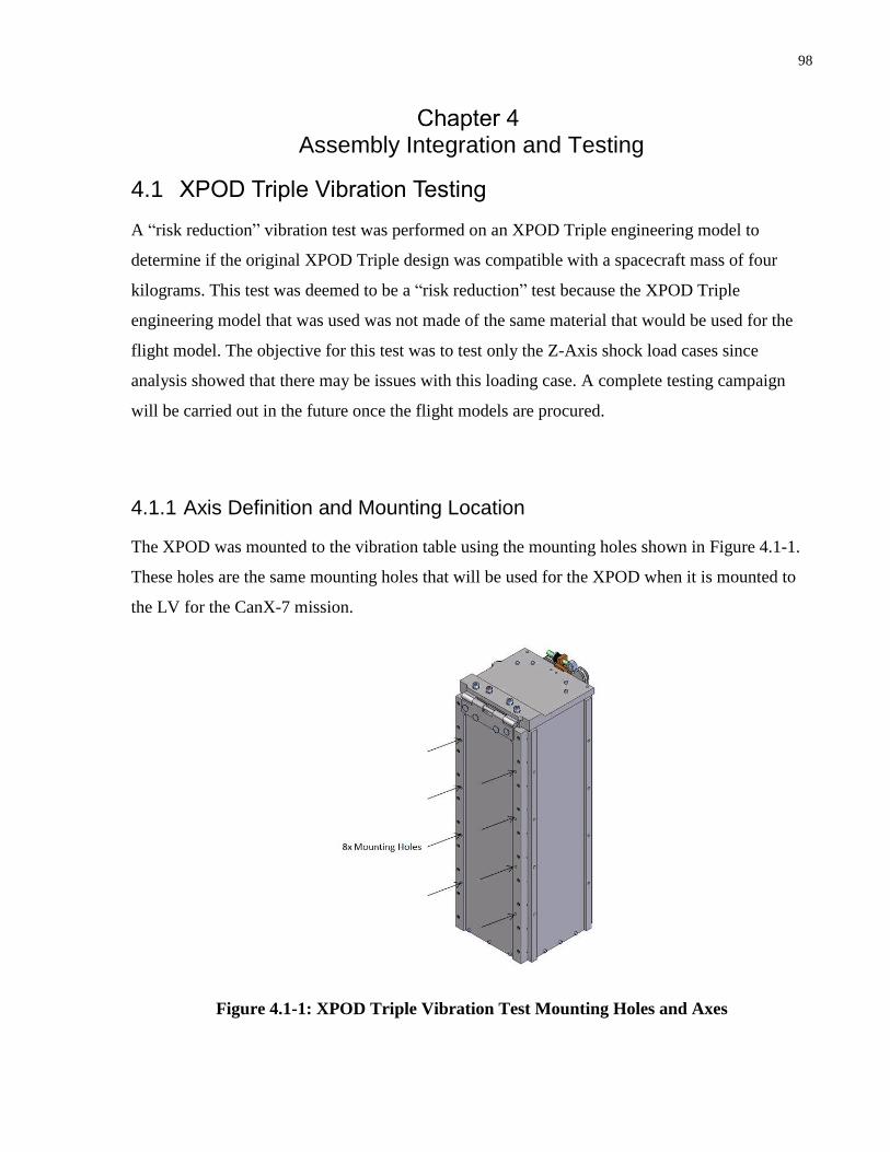
98
Assembly Integration and Testing
4.1 XPOD Triple Vibration Testing
A “risk reduction” vibration test was performed on an XPOD Triple engineering model to
determine if the original XPOD Triple design was compatible with a spacecraft mass of four
kilograms. This test was deemed to be a “risk reduction” test because the XPOD Triple
engineering model that was used was not made of the same material that would be used for the
flight model. The objective for this test was to test only the Z-Axis shock load cases since
analysis showed that there may be issues with this loading case. A complete testing campaign
will be carried out in the future once the flight models are procured.
4.1.1 Axis Definition and Mounting Location
The XPOD was mounted to the vibration table using the mounting holes shown in Figure 4.1-1.
These holes are the same mounting holes that will be used for the XPOD when it is mounted to
the LV for the CanX-7 mission.
Figure 4.1-1: XPOD Triple Vibration Test Mounting Holes and Axes

99
4.1.2 Accelerometer Placement
The accelerometers for the test were placed in the locations shown in Figure 4.1-2 and Figure
4.1-3. Plastic cubes were used for mounting the accelerometers on the test article such that
orthogonal accelerometers could be mounted easily, at the same locations on the structure. The
axes shown in Figure 4.1-2 are the reference axes used for the remainder of the test description.
Figure 4.1-2: Accelerometer Placement Image 1
Figure 4.1-3: Accelerometer Placement Image 2

100
A description of each of the accelerometers is shown in Table 8.
Table 8 - List of Accelerometers
Type Point Location
1 Control Control Fixture plate
2 Measure Cube_1x XPOD Front Panel
3 Measure Cube_1y XPOD Front Panel
4 Measure Cube_1z XPOD Front Panel
5 Measure Cube_2x XPOD Door
6 Measure Cube_2y XPOD Door
7 Measure Cube_2z XPOD Door
8 Measure Cube_3x XPOD Bottom Panel
9 Measure Cube_3y XPOD Bottom Panel
10 Measure Cube_3z XPOD Bottom Panel
The “control” accelerometer was placed on the vibration table mounting plate, and not on the
XPOD. This accelerometer has a different purpose than measuring test data. It is used in the
vibration table closed loop control system such that the vibration table outputs the correct
vibration loads. The rest of the accelerometers were used to collect test data.
An accelerometer was paced on the Front Panel of the XPOD because the Front Panel is well
coupled with the use of screws to the other XPOD panels and is used to characterize the overall
XPOD body motion. An accelerometer was placed on the Door because the door is not as well
coupled to the rest of the XPOD body and information on its motion was desired. Finally, an
accelerometer was placed on the Bottom Panel because possible separations and impacts

101
between the Pusher Plate and Bottom Panel can occur, and information on this event was
desired.
4.1.3 Vibration Levels
This section contains information on the vibration levels that were used.
4.1.3.1 Low-Level Sine Test Levels
As previously mentioned, a low energy sine wave is used as the input to a system under test to
determine the natural frequencies of the structure. Specifically, a 0.5g sine wave is used, that
sweeps in frequency from 10-2000Hz at a rate of two octaves per minute. This allows resonances
in the structure to be measured by the accelerometers that are placed in the various locations on
the structure. The original determination of the natural frequencies is completed by performing a
low-level sine test at the start of the vibration test campaign.
The low-level sine test is also performed before and after major test profiles, such as the shock
test for this vibration campaign. The reason for this is to compare the response characteristics of
the structure from before and after the major vibrations to aid in determining if the structure was
altered by these major vibrations. Slight changes in the responses are typical since settling of the
structure usually takes place as it is subjected to vibrations. However, if major changes occur,
they would be dealt with on a case by case basis where the selected actions depend on the nature
of the change and if any damage is evident on the structure.
4.1.3.2 Shock Test Levels
The vibration profile for the shock test is depicted by the launch vehicle requirements that were
stated in Section 2.1. The profile that is used is a 50g half sine waveform, with a duration of ten
milliseconds. Figure 4.1-4 shows a plot of the waveform’s amplitude over time. This profile was
input into the XPOD Triple structure in both the positive and negative sense in the Z-axis since
analysis showed this to be the loading direction of concern.

102
Figure 4.1-4 – 50g Shock Test Waveform
4.1.4 Inspection Procedure
When performing vibration testing of XPODs, easily comparable images and measurements are
required that will detail whether or not there has been damage, or movement between components
in the XPOD assembly due to the test loading. This section gives a list of images and measurements
that should be gathered before and after the testing campaign for comparative purposes.
4.1.4.1 Image Description Conventions
Section 4.1.4.3 describes images by specifying both a location on the XPOD that should be
imaged, along with the direction that the image should be taken from. For example, Figure 4.1-5
is described as “Overall XPOD From +Z View”. Therefore, the image should be taken of the
XPOD (the entire assembly), from a +Z location.
0
10
20
30
40
50
60
0 1 2 3 4 5 6 7 8 9 10
Time (ms)
Ac
ce
lera
tio
n (
g)

103
Figure 4.1-5: XPOD From +Z View Example Image
4.1.4.2 Measurement Description Convention
The measurements that should be taken as part of the inspection are specified with a description,
a location, along with the axis in which the measurement should be taken in. Figure 4.1-6
illustrates the measurement that should be taken for “Distance Between Door and Front Panel at
–Y Corner in the Z axis” as an example. Note that in Figure 4.1-6 the distance is exaggerated for
the sake of clarity.
Figure 4.1-6: Measurement Example Image
+Y
+X
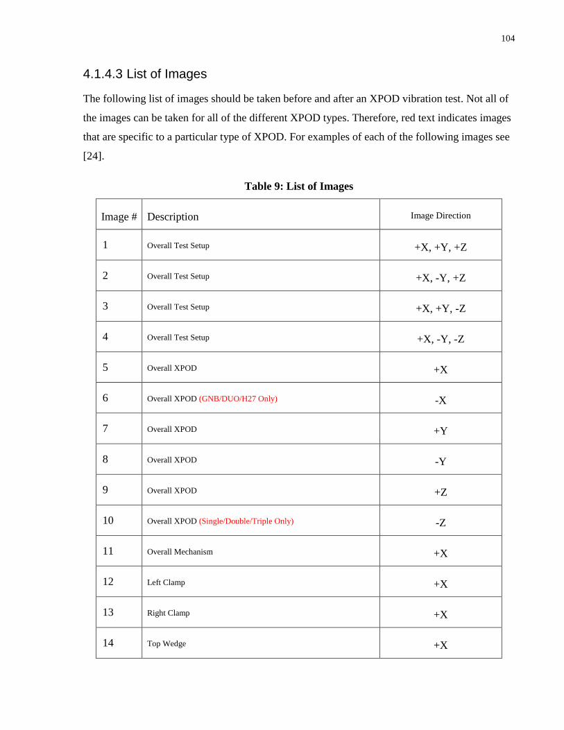
104
4.1.4.3 List of Images
The following list of images should be taken before and after an XPOD vibration test. Not all of
the images can be taken for all of the different XPOD types. Therefore, red text indicates images
that are specific to a particular type of XPOD. For examples of each of the following images see
[24].
Table 9: List of Images
Image # Description Image Direction
1 Overall Test Setup +X, +Y, +Z
2 Overall Test Setup +X, -Y, +Z
3 Overall Test Setup +X, +Y, -Z
4 Overall Test Setup +X, -Y, -Z
5 Overall XPOD +X
6 Overall XPOD (GNB/DUO/H27 Only) -X
7 Overall XPOD +Y
8 Overall XPOD -Y
9 Overall XPOD +Z
10 Overall XPOD (Single/Double/Triple Only) -Z
11 Overall Mechanism +X
12 Left Clamp +X
13 Right Clamp +X
14 Top Wedge +X

105
15 Bottom Wedge +X
16 Interface between Top and Bottom Wedges +X
17 Door to Front Panel Interface – Left side +X
18 Door to Front Panel Interface – Right side +X
19 Door to Front Panel Interface -Y
20 Door to Front Panel Interface +Y
21 Door to Rear Panel Interface (GNB/DUO/H27 Only) -X
22 Door to Rear Panel Interface -Y
23 Door to Rear Panel Interface +Y
24 Hinge (GNB/DUO/H27 Only) -X
25 Hinge +Z
26 Hinge -Y
27 Hinge +Y
28 -Y Door Locking Screw Hole Alignment +Z
29 +Y Door Locking Screw Hole Alignment +Z
30 Top Panel +X+Y Corner +Z
31 Top Panel –X+Y Corner +Z
32 Top Panel –X-Y Corner +Z
33 Top Panel +X-Y Corner +Z
34 Heater Block (Single/Double/Triple Only) -Z

106
35 Heater Block (GNB/DUO/H27 Only) +Z
36 Vectran Line on Countersunk Screw (Single/Double/Triple Only) +X
37 Vectran Line on Eyebolt +X
38 Vectran Line on Eyebolt (Single/Double/Triple Only) +Z
39 Vectran Line on Eyebolt (GNB/DUO/H27 Only) -Z
40 Mechanism Preload Stack +X
41 Mechanism Preload Stack +Z
42 XPOD / S.C Interface @ +X+Y+Z Corner (GNB/DUO/H27 Only) -X, +Y, -Z
43 XPOD / S.C Interface @ -X+Y+Z Corner (GNB/DUO/H27 Only) +X, +Y, -Z
44 XPOD / S.C Interface @ +X-Y+Z Corner (GNB/DUO/H27 Only) -X, -Y, -Z
45 XPOD / S.C Interface @ -X-Y+Z Corner (GNB/DUO/H27 Only) +X, -Y, -Z
46 XPOD / S.C Interface @ +X+Y-Z Corner (GNB/DUO/H27 Only) -X, +Y, +Z
47 XPOD / S.C Interface @ -X+Y-Z Corner (GNB/DUO/H27 Only) +X, +Y, +Z
48 XPOD / S.C Interface @ +X-Y-Z Corner (GNB/DUO/H27 Only) -X, -Y, +Z
49 XPOD / S.C Interface @ -X-Y-Z Corner (GNB/DUO/H27 Only) +X, -Y, +Z
50 Overall XPOD +X, +Y, +Z
51 Overall XPOD +X, -Y, +Z
52 Close-up of Front Panel Sensor Cube Depends on Sensor Placement
53 Close-up of Door Sensor Cube Depends on Sensor Placement
54 Close-up of Bottom Panel Sensor Cube (Single/Double/Triple Only) Depends on Sensor Placement
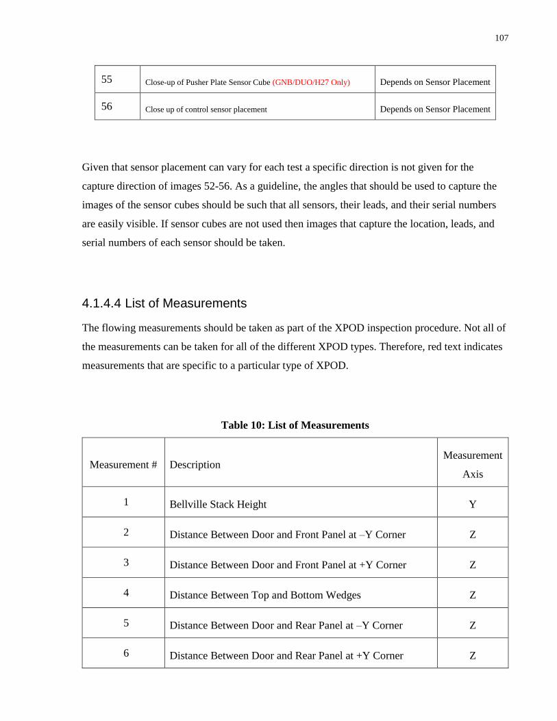
107
55 Close-up of Pusher Plate Sensor Cube (GNB/DUO/H27 Only) Depends on Sensor Placement
56 Close up of control sensor placement Depends on Sensor Placement
Given that sensor placement can vary for each test a specific direction is not given for the
capture direction of images 52-56. As a guideline, the angles that should be used to capture the
images of the sensor cubes should be such that all sensors, their leads, and their serial numbers
are easily visible. If sensor cubes are not used then images that capture the location, leads, and
serial numbers of each sensor should be taken.
4.1.4.4 List of Measurements
The flowing measurements should be taken as part of the XPOD inspection procedure. Not all of
the measurements can be taken for all of the different XPOD types. Therefore, red text indicates
measurements that are specific to a particular type of XPOD.
Table 10: List of Measurements
Measurement # Description Measurement
Axis
1 Bellville Stack Height Y
2 Distance Between Door and Front Panel at –Y Corner Z
3 Distance Between Door and Front Panel at +Y Corner Z
4 Distance Between Top and Bottom Wedges Z
5 Distance Between Door and Rear Panel at –Y Corner Z
6 Distance Between Door and Rear Panel at +Y Corner Z

108
7 Distance Between Flange on Left Clamp and Flange on
Bottom Wedge (Single/Double/Triple Only)
Y
8 Distance Between Flange on Right Clamp and Flange on
Bottom Wedge (Single/Double/Triple Only)
Y
4.1.5 Vibration Test Procedures
The test plan below was used for the XPOD Triple risk reduction test:
1) Mount the XPOD to the slip table in the Z-Axis orientation.
2) Mount the accelerometers on the XPOD and the fixture plate.
3) Take pictures and measurements of the test setup as described in Section 4.1.4.
4) Run the XPOD short form functional test.
5) Run the first Low Level Sine test with an input vibration amplitude of 0.5 g and a
frequency sweep from 10-2000 Hz at a rate of two octaves per minute.
6) Run the 50 g two millisecond half sine test in the +Z direction.
7) Run the 50 g two millisecond half sine test in the -Z direction.
8) Run the second Low Level Sine test with the same parameters as the first Low Level Sine
test.
9) Run the XPOD short form functional test.
10) Take pictures and measurements of the test setup as described in Section 4.1.4.
11) Remove the XPOD from the slip table.
12) Perform the XPOD deployment test.
Following the completion of the XPOD deployment test a visual inspection of the XPOD should
carried out. The photos and measurements that were taken during the test should also be
compared to determine if damage resulted from the test.

109
4.2 EV9 Horizontal Deployment Test
Since the VHF antenna for the EV9 mission has never been flow, or allowed to deploy following
spacecraft deployment from an XPOD, a risk reduction test was completed. The plan for this test
was to use the XPOD ground test vehicle (GTV), a representative mass for the EV9 satellite, and
the EV9 flight XPOD to perform a horizontal deployment of the spacecraft. Typically a flight
XPOD would not be used for risk reduction testing to avoid the risk of damaging flight
hardware. However, because EV9 has slightly different separation system interfaces compared to
other satellites, the EV9 specific XPOD had to be used. The setup can be seen in Figure 4.2-1.
Figure 4.2-1: Overall Test Setup
The representative mass was composed of EV9-A structural components (due to availability of
EV9 components), EV9 structural components, along with several internal GNB component
mass dummies. The magnetometer boom was not included in this test because it would interfere
with the GTV. The UHF antennas were also not included since they are not needed to test the

110
deployment of the VHF antenna and they had not yet been included in a GTV test, which
introduced undesirable risk to the test. However, if the VHF antenna deployment test indicated
possible contact with the UHF antennas during deployment, a subsequent test could be
performed with the UHF antennas included. The VHF antenna that was used was the flight spare
antenna from the EV9 mission and was the same length as the EV9 flight VHF antenna.
One issue with this test was that the flight main spring for the EV9 XPOD was not at SFL for the
test. To work around this a similar spring was used, but the material of this similar spring was
stainless steel and not the same titanium alloy that flight XPOD GNB springs are typically made
of. This caused the stiffness of the spring to be slightly different, but as a representative test, this
was deemed acceptable. The process that was used to estimate the spring constant of the steel
spring is detailed in Section 4.2.1.
The XPOD was actuated without the use of the XPOD firing mechanism for several of the test
deployments such that the test was more easily carried out. However, for the last deployment test
the XPOD was fired using the XPOD actuation mechanism. A more detailed methodology is
given in Section 4.2.2.
4.2.1 Spring Constant Determination Procedure
The procedure that was used to determine the spring constant of the XPOD main spring is given
below:
Step 1) Place the XPOD on a flat surface with the deployment direction facing upwards and with
the door open.
Step 2) Measure the height of the pusher plate above the baseplate at each of the four corners of
the pusher plate. The average of these four values will be the starting height (ℎ𝑠𝑡𝑎𝑟𝑡).
Step 3) Place a known mass (𝑚) in the center on top of the pusher plate to increase the
compression of the main spring.

111
Step 4) Measure the new height of the pusher plate above the base plate at each of the four
corners. The average of these 4 values will be the ending height (ℎ𝑒𝑛𝑑).
Step 5) Estimate the spring constant of the XPOD main spring using:
𝑘𝑠𝑝𝑟𝑖𝑛𝑔 =𝑚𝑔
ℎ𝑠𝑡𝑎𝑟𝑡 − ℎ𝑒𝑛𝑑 (2.61)
where
𝑚 is the mass of the object placed on the pusher plate
ℎ𝑠𝑡𝑎𝑟𝑡 is the height of the pusher plate off of the base plate before the object was
added
ℎ𝑒𝑛𝑑 is the height of the pusher plate off of the base plate after the object was
added
𝑔 is the acceleration due to gravity
4.2.2 Deployment Test Procedure
The procedure that was used to carry out the test deployment of EV9 from its XPOD to
determine the performance of the deployable VHF antenna is given below:
Step 1) Mount the XPOD to the vibration plate. This plate is needed as part of the GTV assembly
to position the XPOD correctly.
Step 2) Attach the GTV to the EV9 representative mass.
Step 3) Attach the GTV XPOD legs to the XPOD as shown in Figure 4.2-1.
Step 4) Clear an area in the lab such that there is enough space to have the spacecraft deploy
Step 5) Lay down the horizontal deployment mat.

112
Step 6) Place the horizontal deployment stand at one end of the mat.
Step 7) Place the vibration plate with the mounted XPOD onto the horizontal deployment stand
such that the horizontal deployment legs are also engaged.
Step 8) Wrap the EV9 VHF antenna around the mass dummy into its “stowed” configuration.
Tape may be needed to temporarily hold the antenna down while sliding the mass dummy
into the XPOD and checking that the spacecraft can move properly in and out of the XPOD.
Step 9) Verify that the EV9 mass dummy slides into and out of the XPOD easily such that the
mass dummy will not get jammed during deployment. It is likely that leveling of the
horizontal XPOD assembly, along with matching the height of the XPOD assembly to the
height of the spacecraft will be necessary to allow the spacecraft to easily slide into and out
of the XPOD. Perform this task by adjusting the 6 adjustable legs in the horizontal XPOD
setup until the spacecraft can easily slide in and out of the XPOD without jamming.
Step 10) Remove the tape from the VHF antenna if it was previously used to hold the antenna
down.
Step 11) Loop a piece of thin Vectran cord through the cutout on the right side of the XPOD
door (See Figure 4.2-2).This cord will be used to hold the door shut.
Figure 4.2-2: Cord Looping Example

113
Step 12) While holding the VHF antenna in its “stowed” configuration slide the spacecraft mass
dummy with the GTV fully into the XPOD in the flight orientation (See Figure 4.2-3) and
close the door. Hold the door shut with the cord that was looped around the door in Step 11).
Figure 4.2-3: Spacecraft in XPOD Orientation
Step 13) Stand behind the XPOD and ensure that when the spacecraft is ejected it will not hit
anything.
Step 14) Set up a recording device such that the deployment can be analyzed. Using a high speed
recording device is preferred since detailed information about the motion of the antenna will
desired after the deployment.
Step 15) Release one end of the looped cord such that the XPOD door can open.
Step 16) After the spacecraft has come to a full stop, stop the recording device.
Step 17) Repeat Step 11) through Step 16) as necessary to collect the required data and to build
up some confidence in the results that are realized. For the final deployment fully arm the
XPOD and deploy the XPOD using the process described in [25].

114
Conclusion
The work that was completed for this thesis included the mechanical design of three
microsatellites and their separation systems. Several missions and design phases were touched
upon while completing this work. Computer modelling along with AIT activities also comprised
a significant portion of the work that was completed.
The XPOD Triple is now at a point where procurement will take place. This was reached by both
analyzing the mechanism in the XPOD, and its main spring. An FEM was also created such that
the structure of the XPOD was deemed acceptable, although not mentioned in this thesis
document. Finally testing of the structure was carried out to ensure that the design was suitable
for the CanX-7 mission, with a bus mass of up to four kilograms.
The MiniMags feasibility study was completed, which involved the creation of a preliminary
structural design that may be used in the future. This design was deemed acceptable by the
payload provider in terms of its mass, power, and volume availability. The bus was also analyzed
such that it was deemed acceptable from a mechanical standpoint with the MiniMags payload.
The EV9 mission was brought from its previous EV9-A design to the current EV9 design. The
tests that were done in ensuring the VHF antenna is compatible with the XPOD ensured that the
risks in using the deployable VHF antenna were acceptable. The flight model of the EV9 bus
was assembled at SFL and testing of the bus to deem that it was built to specification was
successfully completed.
Finally, the NORSAT-1 mission was brought from a proposal level bus design to the PDR level
bus design during the course of the work for this thesis. Trade studies that compared different
bus designs, along with modifications to the layout of the payload appendages took place. The
mechanical design was handed off and is under further development by the current NORSAT-1
mechanical designer.
Overall, appreciable contributions to the mechanical aspects of the above mentioned programs
were made. The mechanical design activities contributed to allowing the structural systems in the

115
above mentioned programs to fulfill their mission requirements. The computer modelling
activities allowed for the verification of these mechanical design requirements before physical
testing could take place, which allowed for iteration of the designs in a time and cost efficient
manner. Finally, the AIT activities that took place brought all of the previously mentioned
missions much closer to being ready for launch and on orbit operation.

116
References
[1] EO Portal, "CubeSat Concept and the Provision of Deployer Services," 2104. [Online]. Available: https://directory.eoportal.org/web/eoportal/satellite-missions/c-missions/cubesat-concept. [Accessed March 2014].
[2] Planatery System Corporation, "Plantery System Corporation Products," 2011. [Online]. [Accessed 14 May 2014].
[3] W. O'Brien, "The Design, Manufacturing, and Testing of eXperimental Push-," University of Toronto, Toronto, 2007.
[4] Space Radiation Analysis Group, Johnson Space Center, "What is space radiation," 22 04 2013. [Online]. Available: http://srag-nt.jsc.nasa.gov/SpaceRadiation/What/What.cfm. [Accessed 07 01 2014].
[5] J. R. Wertz, D. F. Everett and J. J. Puschell, Space Mission Engineering: The New SMAD, Hawthorne: Microcosm Press and Springer, 2011.
[6] C. Dyer, "Radiation Effects on Spacecraft and Aircraft," QinetiQ, Farnborough, 2001.
[7] R. Zee, "Spacecraft Design Presentation," Toronto, 2012.
[8] D. G. Gilmore, Spacecraft Thermal Design Handbook, El Segundo: The Aerospace Press, 2002.
[9] Space Flight Laboratory, NORSAT-1 System Requirements and Verification Matrix v1.0, Toronto: Space Flight Laboratory, 2012.
[10] Antrix Corporation Limited, PSLV User Manual Issue 5, Bangalore, Karnataka, 2007.
[11] Arianespace, Soyuz User's Manual Issue 2 Revision 0, Courcouronnes, 2012.
[12] Arianespace, Ariane 5 User's Manual Issue 4 Revision 0, Courcouronnes: Arianespace, 2004.
[13] S. Mauthe, XPOD Duo Qualificaiton Vibraiton Test Plan, Toronto, Ontario, 2012.
[14] Spaenaur, Spaenaur Catalog 2013, Ontario: Spaenaur, 2013.
[15] R. G. Budynas and J. K. Nisbett, Shigley's Mechanical Engineering Design 9th Edition, New York: McGraw-Hill, 2011.
[16] California Polytechnic State University, CubeSat Design Specification Rev. 12, 2009.
[17] J. Fine, XPOD Tip Off Rate Analysis, Toronto: Space Flight Laboratory, 2014.
[18] B. P. Larouche, Design, Simulation, and Testing of the Structural & Separation System, Toronto: University of Toronto, 2008.
[19] M. Ligori, XPOD H27 Nanosatellite Separation System, Toronto: Space Flight Laboratory, 2011.
[20] B. Brakeboer, GHGSat-D PDR Mechanical Design Document, Toronto: Space Flight Laboratory, 2013.
[21] Siemens, NX 8.0 Help Documentation, 2011.
[22] Hexcel Composites, HexWeb Honeycomb Attributes and Properties, Hexcel, 1999.
[23] MatWeb, "Aluminum 7075-T6; 7075-T651," [Online]. Available: http://matweb.com/search/DataSheet.aspx?MatGUID=4f19a42be94546b686bbf43f79c51b7d&ckck=1. [Accessed 19 February 2014].
[24] J. Fine, "XPOD Inspection Guide for Vibration Testing," Space Flight Laboratory, Toronto, 2013.
[25] M. Ligori, D. Kekez, S. Mauthe and F. Pranajaya, "XPOD GNB Users Guide v 1.4," Space Flight Laboratory, Toronto, 2013.
[26] S. Mauthe, NEMO-HD Mechanical Design Document, Toronto, Ontario, 2013.