Descriptive Statistics for Modern Test Score Distributions ... · PDF fileDESCRIPTIVE...

Running head: DESCRIPTIVE STATISTICS FOR MODERN SCORE DISTRIBUTIONS 1

Descriptive Statistics for Modern Test Score Distributions:

Skewness, Kurtosis, Discreteness, and Ceiling Effects

Andrew D. Ho and Carol C. Yu

Harvard Graduate School of Education

Author Note

Andrew D. Ho is an Associate Professor at the Harvard Graduate School of Education, 455

Gutman Library, 6 Appian Way, Cambridge, MA 02138; email: [email protected]

Carol C. Yu is a Research Associate at the Harvard Graduate School of Education, 407 Larsen

Hall, 14 Appian Way, Cambridge, MA 02138; email: [email protected]

This research was supported by a grant from the Institute of Education Sciences (R305D110018).

The opinions expressed are ours and do not represent views of the Institute or the U.S. Department of

Education. We claim responsibility for any errors.

mailto:[email protected]

mailto:[email protected]

DESCRIPTIVE STATISTICS FOR MODERN SCORE DISTRIBUTIONS 2



Abstract

Many statistical analyses benefit from the assumption that unconditional or conditional distributions are

continuous and normal. Over fifty years ago in this journal, Lord (1955) and Cook (1959) chronicled

departures from normality in educational tests, and Micerri (1989) similarly showed that the normality

assumption is met rarely in educational and psychological practice. In this paper, the authors extend these

previous analyses to state-level educational test score distributions that are an increasingly common target

of high-stakes analysis and interpretation. Among 504 scale-score and raw-score distributions from state

testing programs from recent years, non-normal distributions are common and are often associated with

particular state programs. The authors explain how scaling procedures from Item Response Theory lead

to non-normal distributions as well as unusual patterns of discreteness. The authors recommend that

distributional descriptive statistics be calculated routinely to inform model selection for large-scale test

score data, providing warnings in the form of sensitivity studies that compare baseline results to those

from normalized score scales.




Introduction

Normality is a useful assumption in many modeling frameworks, including the general linear

model, which is well known to assume normally distributed residuals, and structural equation modeling ,

where normal-theory-based maximum likelihood estimation is a common starting point (e.g., Bollen,

1989). There is a vast literature that describes consequences of violating normality assumptions in

various modeling frameworks and for their associated statistical tests. A similarly substantial literature

has introduced alternative frameworks and tests that are robust or invariant to violations of normality

assumptions. A classic, constrained example of such a topic is the sensitivity of the independent-samples

t-test to normality assumptions (e.g., Boneau, 1960), where violations of normality may motivate a robust

or nonparametric alternative (e.g., Mann & Whitney, 1947).

An essential assumption that underlies this kind of research is that the degree of non-normality in

real-world distributions is sufficient to threaten the desired interpretation in which the researcher is most

interested. If most distributions in a particular area of application are normal, then illustrating

consequences of non-normality and motivating alternative frameworks may be interesting theoretically

but of limited practical importance. To discount this possibility, researchers generally include a real-

world example of non-normal data, or they at least simulate data from non-normal distributions that share

features with real-world data. Nonetheless, comprehensive reviews of the non-normality of data in

educational and psychological applications are rare. Almost sixty years ago in this journal, Lord (1955)

reviewed the skewness and kurtosis of 48 aptitude, admissions, and certification tests. He found that test

score distributions were generally negatively skewed and platykurtic. Cook (1959) replicated Lord’s

analysis with 50 classroom tests. Micceri (1989) gathered 440 distributions, 176 of these from large-scale

educational tests, and he described 29% of the 440 as moderately asymmetric and 31% of the 440 as

extremely asymmetric. He also observed that all 440 of his distributions were non-normal as indicated by

repeated application of the Kolmogorov-Smirnov test (𝑝 < .01).


In this paper, we provide the first review that we have found of the descriptive features of state-

level educational test score distributions. We are motivated by the increasing use of these data for both

research and high-stakes inferences about students, teachers, administrators, schools, and policies. These

data are often stored in longitudinal data structures (e.g., U.S. Department of Education, 2011) that

laudably lower the barriers to the analysis of educational test score data. However, as we demonstrate,

these distributions have features that can threaten conventional analyses and interpretations therefrom,

and casual application of familiar parametric models may lead to unwarranted inferences.

Such a statement is necessarily conditional on the model and the desired inferences. We take the

Micerri (1989) finding for granted in our data: these distributions are not normal. At our state-level

sample sizes, we can easily reject the null hypothesis that distributions are normal, but this is hardly

surprising. The important questions concern the magnitude of non-normality and the consequences for

particular models and inferences. We address the question of magnitude in depth by presenting skewness,

kurtosis, and discreteness indices for 504 raw and scale score distributions from state testing programs.

Skewness and kurtosis are well established descriptive statistics for distributions (Pearson, 1895) and are

occasionally used as benchmarks for non-normality (e.g., Bulmer, 1979). We illustrate the consequences

of non-normality only partially. This is deliberate. A complete review of all possible analyses and

consequences is impossible given space restrictions. Thus, our primary goal is to make the basic features

of test score distributions easily describable and widely known. These features may guide simulation

studies for future investigations of the consequences of violating model assumptions. Additionally, if

variability in these features is considerable, this motivates researchers to use an arsenal of diverse

methods to achieve their aims, with which they might manage tradeoffs between Type I and Type II

errors, as well as bias and efficiency.

We have two secondary goals. First, we provide illustrative examples of how these features can

lead to consequential differences for model results, so that researchers fitting their own models to these

data may better anticipate whether problems may arise. Second, we explain the pathology of the non-

normality that we observe in the data. We demonstrate that, when test score distributions are cast as the


results of particular models and scaling procedures, their non-normal features should not be surprising.

We emphasize that non-normality is not inherently incorrect or flawed—it is the responsibility of the

researcher to fit the model to the data, not the reverse. However, if the resulting features are undesirable

for the primary intended use of the test scores, then the procedures that generate the distributions should

be reconsidered.

To accomplish these multiple goals, we present this paper in four parts. The first part introduces

the pathology of non-normality by describing skewness and kurtosis of raw score distributions as natural

properties of the binomial and beta-binomial distributions. This analysis of raw scores serves as a

conceptual link to the Lord (1955), Cook (1959), and Micerri (1989) analyses, which were dominantly

raw-score-based, and sets an historical baseline from which to evaluate modern uses of test scores, which

are scale-score-based, that is, using scores developed using a particular scaling method. In all of the cases

presented here, this scaling method is Item Response Theory (IRT; see Lord, 1980). In the second part,

we present the primary results of the paper in terms of skewness and kurtosis of both raw score and scale

score distributions. We continue to emphasize the pathology of non-normality by describing the

differences between features of raw score and scale score distributions as a consequence of scaling

methods using IRT.

The third part of the paper uses visual inspection of test score distributions to motivate additional

descriptive statistics for scale score distributions. In particular, we motivate statistics that describe the

discreteness of distributions, and we show that visually obvious “ceiling effects” in some distributions are

better identified by discreteness than by skewness. Here, we begin to illustrate simple consequences that

threaten common uses of test scores, including comparing student scores, selecting students into

programs, and evaluating student growth. Finally, in the fourth part of the paper, we describe the possible

impact of non-normality on the results of regression-based test score analyses. We illustrate this with

results from predictive models for students and a “value-added”-type model for school-level scores. For

these sensitivity studies, we compare results estimated using observed distributions to results estimated

using their normalized counterparts. This answers the question, if these distributions were normal, how


would our interpretations differ? Taken together, these arguments build toward a familiar if important

principle: researchers should select models with knowledge of the process that generated the data and

informed by data features, or else risk flawed analyses, interpretations, and decisions.

Data

A search of publicly available state-level test-score distributions yielded 330 scale score

distributions and 174 raw score distributions from 14 different state testing programs in the academic

years ending 2010 and 2011. We constrained the time period to these two years because these state

testing programs were fairly stable at that time and because all states had some data in both years. One of

the programs, the New England Common Assessment Program (NECAP), represents 4 states, Maine,

New Hampshire, Rhode Island, and Vermont, thus the data represent 17 states in total. As Micerri (1989)

noted, the data appropriate for full distributional analyses are rarely publicly available, however, these

states have considerable regional coverage across the United States. We collected distributions from 6

grades (3-8) and 2 subjects (Reading/English Language Arts and Mathematics), for a total of 12 possible

scale score distributions per year.

Raw score distributions were available from 8 of the 14 state testing programs. We use raw

scores largely for illustration, as a historical reference point to previous research, and as a conceptual

reference point to emphasize the consequences of IRT scaling on skewness and kurtosis. Since scores are

generally reported and analyzed using scale scores, the latter half of the paper focuses on scale scores.

Nebraska is missing Mathematics score distributions in 2010, and Oklahoma is missing raw score

distributions in 2010.

Table 1 shows the minimum and maximum number of examinees across the available score

distributions in each state. Unsurprisingly, these numbers are indicators of the relative youth populations

of each state. The distribution with the highest n-count is from Texas with 689938 examinees, and the

distribution with the lowest n-count is from South Dakota with 8982 examinees. Altogether, the

distributions represent data from over 31 million examinees. In the last two columns, Table 1 shows the

minimum and maximum number of discrete score points in the scale score distributions. Distributions


from Colorado are outliers in terms of their counts of discrete score points, with counts around 500 due to

their practice of scoring based on patterns of item responses rather than summed scores (CTB-McGraw

Hill, 2010a, 2011a). Distributions from all other states have discrete score point counts ranging from 28

(New York, Grade 5, English Language Arts, in 2010) to 93 (Texas, Grade 7, Reading, in 2011).

Skewness and Kurtosis

We use skewness and kurtosis as rough indicators of the degree of normality of distributions or

the lack thereof. Unlike test statistics from normality testing procedures like the Kolmogorov-Smirnov 𝐷

or the Shapiro-Wilk 𝑊, skewness and kurrtosis are used here like an effect size, to communicate the

degree of non-normality, rather than statistical significance under some null hypothesis of normality. The

use of skewness and kurtosis to describe distributions dates back to Pearson (1895) and has been reviewed

more recently by Moors (1986), D’Agostino, Belanger, and D’Agostino (1990), and DeCarlo (1997).

Skewness is a rough index of the asymmetry of a distribution, where positive skewness in unimodal

distributions suggests relatively plentiful and/or extreme positive values, and negative skewness suggests

the same for negative values. Skewness is an estimate of the third standardized moment of the population

distribution,

𝑠 =�𝑛(𝑛 − 1)𝑛 − 2

1𝑛∑ (𝑥𝑖 − �̅�)3𝑖

�1𝑛∑ (𝑥𝑖 − �̅�)2𝑖 �

3/2.

Skewness can range from −∞ to +∞, and symmetric distributions like the normal distribution

have a skewness of 0. The 𝑛-based bias correction term for the population estimate is negligible for the

large samples that we have here, but we include it for completeness.

Kurtosis is an estimate of the fourth standardized moment of the population distribution,

𝑘 =𝑛(𝑛 + 1)(𝑛 − 1)(𝑛 − 2)(𝑛 − 3)

∑ (𝑥𝑖 − �̅�)4𝑖(∑ (𝑥𝑖 − �̅�)2𝑖 )2.

Kurtosis can range from 1 to +∞. The kurtosis of a normal distribution is 3. Although it is

common to subtract 3 from 𝑘 and describe this as “excess kurtosis”—beyond that expected from a normal

(1)

(2)


distribution—we use the definition above, where 𝑘 < 3 is platykurtic (less peakedness, weaker “tails,”

heavy “shoulders”), and 𝑘 > 3 is leptokurtic (more peakedness, heavy tails, weak shoulders). As

references, a uniform distribution has a kurtosis of 1.8 (platykurtic), and a logistic distribution has a

kurtosis of 4.2 (leptokurtic).

Part 1: Raw Score Distributions

In this section, we begin to demonstrate that the non-normal features of test score distributions are

the byproducts of well-established models and scaling procedures. Lord (1955) and Cook (1959) report

two findings: (1) raw score distributions from “easy” tests generally have negative skew, and (2)

symmetric raw score distributions tend to be platykurtic (kurtosis < 3)1. They both operationalized the

“easiness” of a test as the mean raw score over the maximum possible score. This is equivalent to the

average of item proportions correct, �̅�, where “easy” tests have �̅� > 0.5. Figure 1 replicates their findings

empirically. The skewness and kurtosis of raw score distributions are plotted on a scatterplot in light gray

and are concentrated in the lower left of the plot. All 174 raw score distributions meet the Lord-Cook

definition of “easy,” where the minimum �̅� across 174 distributions is 55.41% (not shown). Figure 1

shows that all raw score distributions, in light gray, have negative skew. In addition, Figure 1 shows that

the raw score distributions that are closest to 0 skew are all platykurtic, with kurtosis < 3.

These findings are straightforward to explain in terms of models for test score distributions that

have become well established since the publication of the Lord (1955) and Cook (1959) reviews. Even

from a naïve model for test scores that assumes all item difficulties are the same (all 𝑝𝑖 = 𝑝), we can

demonstrate that easy tests will have negatively skewed score distributions using a binomial model, which

has a known skewness of,

𝑠𝑏𝑖𝑛𝑜𝑚𝑖𝑎𝑙 =1 − 2𝑝

�𝑖𝑝(1 − 𝑝).

1 Both Lord(1955) and Cook (1959) operationalized skewness and kurtosis using percentile-based statistics (e.g., skewness as (𝑃90 + 𝑃10)/2 − 𝑃50). We use the modern definitions of skewness and kurtosis specified in Equations 1 and 2. We also replicated results using the percentile-based definitions of skewness and kurtosis, and they do not change any substantive conclusions.


Here, 𝑝 is the common item difficulty, and 𝑖 is the number of items on the test. For any 𝑝 > .5,

the skewness will be negative, consistent with the first Lord-Cook finding.

Given that item proportions correct 𝑝𝑖 are not constant across items in practice, a more

appropriate model for raw score distributions is the beta-binomial distribution, where the distribution of

item proportions correct 𝑝𝑖 is modeled by a 2-parameter beta distribution. The beta distribution for 𝑝𝑖 is

defined by parameters 𝛼 and 𝛽, where the mean of the distribution of 𝑝𝑖 will be 𝜇𝑝 = 𝛼𝛼+𝛽

.

We can use the beta-binomial model to explain the second Lord-Cook finding: symmetric raw

score distributions tend to be platykurtic. To illustrate this, we constrain the 𝛼 and 𝛽 parameters that

control the beta distribution of 𝑝 values to sum to 4. This constrains 𝛼 and 𝛽 for any chosen 𝜇𝑝, for

example, if 𝜇𝑝 = 0.75, then 𝛼 = 3 and 𝛽 = 1. We then assume a 50-item test, consistent with a central

number of discrete score points from Table 1.

Next, given the known expressions for the skewness and kurtosis of the beta-binomial distribution

(these expressions are complex and add little insight, so we defer to statistical reference texts), we can

establish a theoretical relationship between skewness and kurtosis under these constraints. This

relationship is shown as a dashed line in Figure 1 for various levels of 𝜇𝑝. As Figure 1 shows, a

symmetric distribution (modeled as beta-binomial when 𝜇𝑝 = 0.5 and 𝛼 = 𝛽 = 2) is platykurtic with

kurtosis < 3. Similarly, the location of raw score distributions on and around the dashed line in Figure 1

shows that the skewness and kurtosis of raw score distributions is well explained by a beta-binomial

model parameterized by 𝜇𝑝. Easier tests with higher 𝜇𝑝 will be negatively skewed. Symmetric tests will

be platykurtic. And harder tests with lower 𝜇𝑝 will be positively skewed.

Although alternative constraints (for 𝛼 and 𝛽 in terms of 𝜇𝑝) and more flexible models for test

scores (like the 4-parameter beta-binomial model; Hanson, 1991) are available, this illustration suffices to

demonstrate that the Lord-Cook skewness and kurtosis findings are consistent with the known behavior of

well-established models for raw score distributions. Raw score distributions will be non-normal to the

degree that they are easier or harder for their respective populations. They will also become progressively


more leptokurtic as the average difficulty ranges away from 50%. If raw score distributions are the target

of analysis and model results are known to be sensitive to skewness, for example, concerns will arise only

if the test is quite easy or quite hard for its respective population.

Part 2: Skewness and Kurtosis of Scale Score Distributions

In this section, we transition our focus from indices of non-normality of raw score distributions to

indices of non-normality of scale score distributions. The theoretical and practical benefits of modern

scaling methods, most notably those deriving from Item Response Theory (Lord, 1980; Yen &

Fitzpatrick, 2006), are substantial, and raw scores are no longer the basis for most large-scale test score

scaling and reporting. This motivates a review of scale score distributions, which are shown in black in

Figure 1. Although about half of scale score distributions do not have a raw score counterpart, we can see

that the effect of IRT scaling on skewness and kurtosis is generally a balancing of skewness and an

increase in kurtosis. We explain the pathology of this effect later in this section.

Table 2, which overviews median, minimum, and maximum skewness and kurtosis of

distributions for each state, also reflects this tendency, as states that have both raw and scale scores show

median skewness generally balancing toward 0 from raw to scale scores, and median kurtosis generally

increasing from raw to scale scores. Across all states, median skewness for raw scores is negative and

median kurtosis for raw scores is less than 3, and median skewness for scale scores is negligibly positive,

and median kurtosis for scale scores is greater than 3. New York is separated by academic year, because,

unlike other states, the distributions of skewness and kurtosis differed substantially across years. Figure 2

also shows box plots representing distributions of skewness and kurtosis by state. Note that there is a

very strong state effect on skewness and kurtosis indices; these distributional features are very similar

within states—even across grades and subjects—and very different among states.

Table 2 and Figure 2 show that Colorado and New York are outlying states in terms of skewness

and kurtosis, with median distributions in Colorado and New York in 2011 showing considerable

negative skew, and median distributions in New York in 2010 showing considerable positive skew. Both

show heavily leptokurtic distributions. The most negatively skewed Colorado distributions happen to be


from the Reading tests and are more heavily skewed in lower grades. In New York, most of the skewed

distributions happen to be from the reading test, as well.

Here, we continue with an effort to describe the pathology of the non-normal features of score

distributions, in this case, scale score distributions. State-by-state explanation of the reasons for particular

levels of skewness and kurtosis is beyond the scope of this paper. Such explanation would require item-

level data and/or particular knowledge of scaling practices that are not always available in public

technical reports. As we noted earlier, there is also nothing inherently incorrect or flawed about score

distributions with extreme levels of skewness and kurtosis, as long as they arise from a defensible scaling

and linking procedure that supports accurate user interpretations of scores and successive differences

between scores. Nonetheless, we review three factors that may help to explain how these extreme values

of skewness and kurtosis arise operationally.

First, most operational scoring procedures produce a 1-to-1 mapping of summed “number

correct” scores to scale scores (Yen & Fitzpatrick, 2006). These mappings align with student and teacher

intuition about the scoring of classroom tests but may sacrifice useful information deriving from patterns

of item responses. Some 1-to-1 mappings derive naturally from simple IRT models like the 1-parameter

logistic model. Other scoring methods, like “inverted test characteristic curve (TCC)” approaches (Yen,

1984), operate similarly to a logit transformation of percentage-correct scores,2 such that high and low

scores are stretched to extremes. This naturally increases kurtosis, consistent with the differences

between raw-score and scale-score kurtosis shown in Figure 1 and Table 2. When there are

disproportionate frequencies at high or low scores, these transformations may result in positive or

negative skew, respectively. This procedure was used in New York and represents an explanation for the

considerable skewness and kurtosis of New York score distributions.

Second, many scoring approaches have undefined perfect and zero scores (in the case of

maximum likelihood estimation in IRT), and others also have undefined scores below chance (in the case

2 Lord (1980) showed that, for 1- and 2-parameter logistic IRT models, maximum likelihood estimates of proficiency parameters are in fact a linear function of logit-transformed percentage-correct scores, in the special case when items are functionally equivalent.


of inverted TCC approaches). In these cases, a lowest and highest obtainable scale score (LOSS and

HOSS, respectively) is determined judgmentally or by some established extrapolation procedure (e.g.,

Kolen & Brennan, 2002). The selection and location of these scores can affect skewness and kurtosis,

especially when large percentages of examinees obtain perfect scores or scores below chance. In general,

when they are extreme compared to the rest of the distribution, kurtosis will increase, and distributions

will be relatively skewed when densities are imbalanced toward either LOSS or HOSS. When HOSS and

LOSS are forced to be equal over many years or across multiple grades, the linking constraints can draw

distributions farther from HOSS and/or LOSS, and this would also affect skewness and kurtosis. We

return to this topic in the next section.

Third, certain year-to-year and grade-to-grade linking approaches may affect skewness and

kurtosis. Linking that relies on linear transformations, such as mean-sigma linking and characteristic

curve linking (e.g., Kolen& Brennan, 2002), will not affect skewness and kurtosis any more than the

separate IRT calibrations upon which they are based. However, constrained or concurrent calibration

(e.g., Yen & Fitzpatrick, 2006), where parameters of item characteristic curves are constrained to or

simultaneously estimated with those from previous years or different grades, may lead to distributions

with extreme skewness and kurtosis. This may manifest in distributions that are systematically more

skewed across grade levels or over time. Incidentally, this is the pattern that arises in Colorado, where

skewness is greater toward the lower grades (not shown).

Our intent in reviewing these procedures is to explain why some score distributions in some states

may exhibit different or particularly extreme skewness and kurtosis values. Again, we emphasize that

non-normality is a feature and not necessarily a flaw. Test designers may reconsider the use of particular

scoring procedures if this degree of non-normality threatens intended test score uses. For secondary

analysts, any resulting non-normality must be handled with the usual iterative model fitting and

diagnostic process, with the use of sensitivity studies where appropriate.

Part 3: Discreteness and Ceiling Effects


The skewness of variables is used not only as an index of non-normality but also as an index for

“ceiling effects” or “floor effects,” where positively skewed variables are assumed to have a floor effect,

and negatively skewed variables are assumed to have a ceiling effect (e.g., Koedel & Betts, 2010).

Ceiling and floor effects are also assumed whenever data are censored, that is, when the locations of

scores above or below a particular ceiling/floor are not known, and they are only known to be at or

above/below that score. Whereas non-normality may motivate robust or nonparametric procedures, these

censored data motivate tobit regression and other censored data models (Long, 1997; Tobin, 1958).

We define ceiling and floor effects as insufficient measurement precision to support desired

distinctions between examinees at the upper and lower regions of the score scale, respectively. In this

section, we argue that skewness is neither sufficient nor necessary for ceiling or floor effects. We then

present some simple descriptive statistics that highlight unusual features of modern test score distributions

that are akin to ceiling and floor effects—features that skewness and kurtosis alone do not capture.

Finally, we provide illustrative examples of consequences of this discreteness in common, practical uses

of test scores.

We begin by demonstrating that a strongly skewed distribution may nonetheless retain

measurement precision in score regions that seem to be compressed. A well-established feature of

logistic IRT scales is conditional standard errors of measurement that are smallest for central scores and

largest at extremes. This contrasts with conditional standard errors of measurement for raw scores, which

are largest for central scores and smallest at extremes (Haertel, 2006). Following Lord (1980), we

consider an IRT-based scoring procedure that results in a symmetric distribution on some score scale 𝜃.

Next, we consider a nonlinear monotonic transformation to an alternative score scale 𝜃∗, for example, an

exponential transformation that results in a relative compression of low scores and a relative stretching of

high scores. This results in a positively skewed distribution and, arguably, a floor effect.

As Lord (1980) demonstrates, however, information at any score point on the scale of 𝜃∗ is

proportional to �𝑑𝜃∗

𝑑𝜃�−2

, which will be relatively high where the score scale 𝜃∗ is compressed compared


to 𝜃. Although the low end of a score scale may be relatively compressed under the transformation, the

conditional standard error will decrease as a result. This demonstrates that compression of a score scale is

not necessarily synonymous with a loss of information in the compressed region. In short, a skewed

distribution is not sufficient to indicate a ceiling or floor effect.

In Figure 3, we also demonstrate that skewed distributions are not necessary for ceiling or floor

effects. To construct Figure 3, we listed all distributions with skewness between ±0.1 and kurtosis

between 2.75 and 3.75, that is, fairly symmetrical distributions with little excess kurtosis. Of these 46

distributions, we selected 6 illustrative discrete histograms of scale score distributions from a range of

states, grades, and subjects. Figure 3 shows that all 6 of these distributions show one interesting feature:

extremely sparse score points toward the positive extremes of the score scale. Notably, these distributions

do not appear symmetric at a glance. This is something of an optical illusion, where it is difficult to

reconcile the coarseness and fineness of the spacing between adjacent score points, on the one hand, with

the percentage of examinees at each score point on the other.

Although this is a purposeful sample, these are not outlying distributions; many additional

symmetric (and asymmetric) distributions also show this feature. We use these distributions to illustrate

that it is often discreteness at the positive ends of the score scale—in particular, a small number of score

points distinguishing between large percentages of examinees—that can raise concerns about ceiling

effects, even in cases where distributions are symmetric, as measured by skewness, and do not show

excess kurtosis. If test score users wish to distinguish among the highest 5-10% of high-scoring

examinees in these distributions, such distinctions would be difficult or impossible to justify. This

demonstrates that skewness is not necessary for ceiling effects. These features are more consistent with a

definition of ceiling effects that relates to censored data.

Figure 4 provides descriptive statistics that further illustrate the sparseness of discrete score

points at the positive end of the score scale. The top tile of the figure shows the actual count of discrete

score points that distinguish among the top 10% of examinees. For example, if more than 10% of

examinees are located in the single top score point, then this count is 1. If 5% are in the top score point


and 6% are in the second highest score point, then this count is 2. Figure 4 shows that many states have

only a few score points distinguishing among the top 10% of examinees. Some distributions in New

York and Texas have only 1 score point distinguishing among the top 10% (that is, there is no distinction

at all), and the Texas, New York (in 2000), and Idaho median number of distinguishing score points is 2,

3, and 4, respectively.

The middle tile of Figure 4 shows the percentage of total discrete score points that distinguish

among the top 10% of examinees. Although it may seem that a small percentage of score points that

distinguish in this range is reasonable, it is worth referencing this to what is expected for discrete

unimodal distributions. If we define a discrete standard normal distribution as one that divides the range

[−𝑐, 𝑐] into evenly spaced bins undergirding a normal distribution, then the expected percentage of

discrete score points that distinguish among the bottom or top proportion 𝑞 of examinees is given by:

Φ−1(𝑞)+𝑐2𝑐

, where Φ−1 is the inverse normal cumulative distribution function. This percentage is 28.64%

when the discrete score bins range from -3 to +3 and desired distinctions are among the top 10% (𝑐 = 3

and 𝑞 = .1). As Figure 4 shows, the proportion of discrete score bins distinguishing the top 10% is far

less than expected under this discrete normal model. On the other side of these distributions, the

proportions of discrete score bins distinguishing the bottom 10% are far greater than expected in almost

all states (not shown).

The top two tiles of Figure 4 are specific instantiations of a general question: What percentage of

examinees is distinguished by what number (or percentage) of discrete scores? Although we chose the top

10%, any other percentage leads to the same conclusion: the higher ends of modern scale score

distributions have larger percentages of examinees than those at the lower ends. We consider this to be a

kind of asymmetry that derives from the discrete binning of scores. This asymmetry can arise even when

score distributions are not skewed, as Figure 3 demonstrates.

A useful way to conceptualize this is to recognize that, if the scale score points were equally

spaced, the distributions would be negatively skewed. For 1-to-1 score mappings, this equally spaced


scale is equivalent to the raw score scale. This therefore represents a restatement of the Lord-Cook

finding from a Part 1: tests are generally “easy” (�̅� > 0.5), thus distributions are negatively skewed. The

fact that many distributions are nevertheless “symmetric” as determined by skewness reflects that there

are two features of these distributions that are in balance. The first is the disproportionate density of

examinees in higher score points. The second is the relative stretching of the higher region of the score

scale. For the symmetric distributions that we show in Figure 3, these two features offset.

The third tile in Figure 4 highlights this second feature more dramatically, by describing the

isolation of the highest score point in terms of standard deviation units. This last tile is akin to answering

the question, what is the difference between getting the second highest score and the highest score, in

standard deviation units? As Figure 3 already illustrates, the highest score point can often be very

isolated. Figure 4 shows that the highest score point is often more than a full standard deviation unit from

the second highest score.

As we have stated earlier, our purpose is primarily to describe the features of score distributions

and secondarily to illustrate the consequences across the space of possible analyses. Figures 3 and 4

highlight features of score distributions that we do not believe are well appreciated. Whereas score points

for raw score distributions are evenly spaced and bounded, scale score distributions are far sparser at their

upper ends and occasionally have outlying positive extremes due either to HOSS decisions or chosen IRT

scoring procedures. Raw score distributions are generally well summarized by skewness and kurtosis

given their evenly spaced score points. In contrast, the symmetry of scale score distributions is a

confounded interplay between disproportionate density and uneven spacing between discrete score points.

We have provided illustrations and simple descriptive statistics that begin to capture these peculiar

features.

We now turn toward the secondary goal of illustrating the consequences of this discreteness, in

order to provide cues for others to recognize when their research question or procedure may be threatened

by common features of scale score distributions. Three examples of simple, practical consequences

follow directly from Figure 3. The first example arises in the context of individual score reporting. The


bottom tile of Figure 3 shows that the scale score difference between two students, one with a perfect

score and one who answers a single item incorrect, can be greater than 1 standard deviation in 8 states,

and greater than 2 standard deviations in 3 states. For students, parents, and teachers, the idea that getting

one more item correct would result in the equivalent of, say, 100 to 200 SAT score points, would be at

least confusing and very likely controversial.

The second example concerns a common secondary use of educational test scores: selection into

special programs. As one example, gifted programs commonly use a percentile-rank-based cutoff as a

partial or sole criterion for eligibility, sometimes the 90th percentile, and sometimes the 95th or 96th (e.g.,

McGinley, Herring, & Zacherl, 2013). If the norm group for these percentiles were the empirical

distribution, there are distributions in New York and Texas where these three percentiles would be

literally indistinguishable—they would refer to the exact same score, because the highest score point in

some of these distributions contains more than 10% of students. If the norm group for these percentiles is

a national norm group or any other reference group, then the percentile-rank-based inference may be

correct on average, but there would likely be dramatic practical consequences depending upon whether

the heavily loaded top score point happened to be located above or below the cutoff.

The third example is an extension of the first that highlights the increasingly common use of

educational score scales to support interpretations about student growth. If we interpret the scale

underlying the distributions in Figure 3 as a vertical scale capable of supporting repeated measures on the

same students, raw score gains in the lower regions of the score scale are dramatically underemphasized

on the IRT score scale, and raw score gains in the upper regions are dramatically overemphasized. The

fact that different raw score differences map to different scale score differences is hardly noteworthy.

However, the degree shown in Figures 3 and 4 is striking and threatens superficial “face” validity. There

may be statistical warrant for a 1-raw-score-point gain at the top of the scale equaling a 10-raw-score-

point gain at the bottom, but rarely is modern test score usage accountable to statistical criteria alone.

Part 4: Consequences of skewness on regression-based analyses.


This section continues the illustration of consequences by describing the magnitude of the impact

of non-normality on common regression-based uses of test scores. The first use considered is simple

linear prediction, and the second is the estimation of so-called “value added” effects (McCaffrey,

Lockwood, Koretz, Louis, & Hamilton, 2004). To establish a reference for comparison, we normalize

score distributions, reducing their skewness and excess kurtosis. By comparing target statistics estimated

from observed and normalized data, we obtain the starkest answer to the question: if these data were

normal, what difference would it make for this particular analysis and interpretations therefrom?

For this real data example, we use a longitudinal, student-level dataset from a large eastern state.

Five grade cohorts have available data across two consecutive years, resulting in five examples of two-

timepoint analyses. Note that this analysis requires student-level linkages facilitating longitudinal

analysis—these are not publicly available data. The target statistics that signal possible substantive

consequences is twofold: the difference between grade-to-grade correlations from observed vs.

normalized data, and the correlation between school effects estimated from observed vs. normalized data.

School effects are school-level averages of student-level residuals (e.g., Chetty, Friedman, & Rockoff, in

press) from a simple linear regression model. We also obtain shrinkage estimates from a model with

school random effects (e.g., Rabe-Hesketh & Skrondal, 2012), but the practical difference in terms of our

outcomes of interest are inconsequential, and we opt for the simpler metric for its transparency and its

straightforward replicability.

Given 2010 (𝑥) and 2011 (𝑦) scores from student 𝑖 and school 𝑗, we estimate separately for each

grade:

𝑦𝑖𝑗 = 𝛽0 + 𝛽1𝑥𝑖𝑗 + 𝜖𝑖𝑗

𝜖𝑖𝑗~𝑁(0,𝜎𝜖2)

Without loss of generality, we assume 𝑦𝑖𝑗 and 𝑥𝑖𝑗 are already standardized, thus 𝛽1 = 𝜌𝑥𝑦, the

grade-to-grade correlation of interest, and �̂�2 = 𝑟𝑥𝑦2 = 𝑅2, the proportion of variance in 𝑦 accounted for

by 𝑥. For school effects, we take student-level residuals, 𝑒𝑖𝑗 = 𝑦𝑖𝑗 − 𝑦�𝑖𝑗 , and average them at the school


level, by school membership in 2011. The �̅�𝑗 are the school-level statistics of interest for each grade

cohort (studentization of residuals is also inconsequential given these sample sizes). Table 3 shows

sample sizes for students and schools, for schools with grade cohort sizes of 30 or more (around 90% of

schools and 98% of students). The observed skewness and kurtosis of the 2010 and 2011 score

distributions are also shown.

To normalize score distributions, we assign each score the normal deviate corresponding to the

percentile rank of the score. Let 𝑟𝑥 be the rank of score 𝑥, where tied values are all assigned their average

rank. The normalized score is Φ−1 �𝑟𝑥−0.5𝑛𝑖

�, where the Hazen correction is used to avoid untransformable

percentile ranks of 0 or 100 (Barnett, 1975). Table 3 also shows the skewness and kurtosis of normalized

distributions. Distributions will not be perfectly symmetrical or mesokurtic due to their discreteness.

The first outcome of interest is the difference between 𝑟𝑥𝑦 from observed vs. normalized data. As

expected, the correlation is higher when score distributions are normalized. The practical significance of

this from an interpretive standpoint is interpretable in terms of this statistic alone: one standard deviation

unit difference in 𝑥 predicts a .64 standard deviation unit difference in 𝑦 under observed scores but a .75

standard deviation unit difference under normalized scores. Non-normality generally degrades

correlations and predictions (in terms of 𝑅2, easily calculated from Table 3). As longitudinal analyses

increasingly have consequences for individual reporting, including the prediction of future attainment

using growth models (e.g., Castellano & Ho, 2013a), conventional predictive models will underperform

on predictive performance unless they accommodate the non-normality of these data.

The second outcome of interest is the correlation between the �̅�𝑗 for normalized and observed

scale scores, 𝑟�̅�𝑗𝑛𝑜𝑟𝑚,�̅�𝑗𝑜𝑏𝑠 . In addition, for illustration, we report percentiles from the distribution of

absolute differences in school percentile rank. Each absolute difference in percentile rank answers the

question, how many percentile ranks, in the distribution of school �̅�𝑗, would a school change, if we

switched from observed scores to normalized scores? Table 3 shows that the correlations range from .96

to .99 across different grade cohorts.


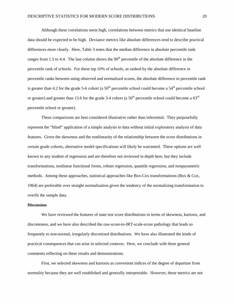
Although these correlations seem high, correlations between metrics that use identical baseline

data should be expected to be high. Deviance metrics like absolute differences tend to describe practical

differences more clearly. Here, Table 3 notes that the median difference in absolute percentile rank

ranges from 1.5 to 4.4. The last column shows the 90th percentile of the absolute difference in the

percentile rank of schools. For these top 10% of schools, as ranked by the absolute difference in

percentile ranks between using observed and normalized scores, the absolute difference in percentile rank

is greater than 4.2 for the grade 5-6 cohort (a 50th percentile school could become a 54th percentile school

or greater) and greater than 13.6 for the grade 3-4 cohort (a 50th percentile school could become a 63rd

percentile school or greater).

These comparisons are best considered illustrative rather than inferential. They purposefully

represent the “blind” application of a simple analysis to data without initial exploratory analysis of data

features. Given the skewness and the nonlinearity of the relationship between the score distributions in

certain grade cohorts, alternative model specifications will likely be warranted. These options are well

known to any student of regression and are therefore not reviewed in depth here, but they include

transformations, nonlinear functional forms, robust regression, quantile regression, and nonparametric

methods. Among these approaches, statistical approaches like Box-Cox transformations (Box & Cox,

1964) are preferable over straight normalization given the tendency of the normalizing transformation to

overfit the sample data.

Discussion

We have reviewed the features of state test score distributions in terms of skewness, kurtosis, and

discreteness, and we have also described the raw-score-to-IRT-scale-score pathology that leads so

frequently to non-normal, irregularly discretized distributions. We have also illustrated the kinds of

practical consequences that can arise in selected contexts. Here, we conclude with three general

comments reflecting on these results and demonstrations.

First, we selected skewness and kurtosis as convenient indices of the degree of departure from

normality because they are well established and generally interpretable. However, these metrics are not


universally embraced, and expressions of the magnitude of non-normality are still not as commonly

understood as, for example, expressions of the magnitude of effects in meta-analysis (Cohen, 1988;

Hedges & Olkin, 1985). It is just as difficult and necessarily contextual to determine whether a .5

standard deviation unit effect is small, medium, or large as it is to determine whether a skewness of .5 is

mildly skewed, moderately skewed, or heavily skewed, but there is far more effort toward the former and

far less effort toward the latter. We look forward to greater understanding around metrics that attempt to

describe the magnitude of non-normality and associated consequences in particular contexts.

Second, nonetheless, skewness and kurtosis seem useful as indices to facilitate study of violating

assumptions in many cases. Formally, Yuan, Bentler, and Zhang (2005) provide a nice primer on the

known effects of skewness and kurtosis upon inference for the mean and variance in the univariate case,

and they generalize from there to discuss implications for multivariate covariance structure analysis.

Practically, Castellano & Ho (2013b) compare quantile-regression-based Student Growth Percentiles

(SGPs; Betebenner, 2009) to more parametric alternatives across varying levels of skewness and find that

SGPs begin to dominate at particular levels of skewness. Theoretically, distributions like the skew-

normal (Azzalini & Capitanio, 1999) allow for simulations to study the consequences of violating normal

assumptions in terms of skewness in controlled conditions. The concept of skewness and, to a lesser

degree, kurtosis, is likely to remain useful in indexing non-normality.

Third, we used Figure 3 to motivate the consideration of discreteness, particularly the common

pattern whereby intervals between score points are sparser at high ends of distributions. We observed that

these features can be explained as the result of easy tests that generate a negatively skewed raw score

distribution, along with a scaling and scoring model that resembles a logistic transformation in its

practical consequences. Notably, the rise of the Common Core State Standards in state and federal policy

in the United States (Porter, McMaken, Hwang, & Yang, 2011) is likely to increase the “rigor” of state

tests in the near term. This purported rigor will largely arise from changes to content standards, as well as

changes to the judgmentally determined cut scores that determine “proficiency.” However, to the extent

that rigor manifests in more central average item percentages correct, �̅�𝑖 ≈ 0.5, our analysis suggests that


more apparently symmetric discrete distributions will result, with smaller percentages at high score points

and less spacing between these points. This may have the unintended benefit of ameliorating the

problems of individual score reporting, selection into programs, and interpretation of gains that we

described in Part 3. More generally, we hope that irregular discreteness, whether or not it is described as

a ceiling effect, continues to receive attention as a byproduct of the practical application of IRT scaling

methods and as a possible threat to particular uses of test scores.


References

Azzalini, A., & Capitanio, A. (1999). Statistical applications of the multivariate skew normal

distribution. Journal of the Royal Statistical Society. Series B (Statistical Methodology), 61, 579-

602.

Boneau, C. A. (1960). The effects of violations of assumptions underlying the t test. Psychological

Bulletin, 57, 49-64.

Bulmer, M. G. (1979). Principles of statistics. New York: Dover.

Box, G. E. P. and Cox, D. R. (1964). An analysis of transformations. Journal of the Royal Statistical

Society, Series B, 26, 211-252.

Castellano, K. E., & Ho, A. D. (2013a). A practitioner’s guide to growth models. Report commissioned

by the Council of Chief State School Officers.

Castellano, K. E., & Ho, A. D. (2013b). Contrasting OLS and quantile regression approaches to Student

“Growth” Percentiles. Journal of Educational and Behavioral Statistics, 38, 190-215.

Cohen, J. (1988). Statistical Power Analysis for the Behavioral Sciences. Hillsdale, New Jersey:

Lawrence Erlbaum Associates.

Cook, D. L. (1959). A replication of Lord's study on skewness and kurtosis of observed test-score

distributions. Educational and Psychological Measurement, 19, 81-87.

CTB McGraw-Hill. (2010a). CSAP Technical Report 2010 – Tables. (Colorado Student Assessment

Program Technical Report 2010). Retrieved from

http://www.cde.state.co.us/assessment/documents/reports/CSAP_2010_TECHNICAL_REPORT.zip

CTB/McGraw-Hill. (2010b). Appendix I – Scale Score Frequency Distributions. (New York State Testing

Program 2010: Mathematics, Grades 3-8). Retrieved from

http://www.p12.nysesd.gov/assessment/reports/2010/math-techrep-10.pdf

CTB/McGraw-Hill. (2010c). Appendix J – Scale Score Frequency Distributions. (New York State Testing

Program 2010: English Language Arts, Grades 3-8). Retrieved from

http://www.p12.nysed.gov/assessment/reports/2010/ela-techrep-10.pdf


CTB McGraw-Hill. (2011a). CSAP Technical Report 2011 – Tables. (Colorado Student Assessment

Program Technical Report 2011). Retrieved from

http://www.cde.state.co.us/assessment/documents/reports/CSAPTechReport.zip

CTB/McGraw-Hill. (2011b). Appendix G – Scale Score Frequency Distributions. (New York State

Testing Program 2011: Mathematics, Grades 3-8). Retrieved from

http://www.p12.nysed.gov/apda/reports/ei/tr38math-11.pdf

CTB/McGraw-Hill. (2011c). Appendix H – Scale Score Frequency Distributions. (New York State

Testing Program 2011: English Language Arts, Grades 3-8). Retrieved from

http://www.p12.nysed.gov/apda/reports/ei/tr38math-11.pdf

D'Agostino, R. B., Belanger, A., & D'Agostino, R. B., Jr. (1990). A suggestion for using powerful and

informative tests of normality. American Statistician, 44, 316-321.

DeCarlo, L. T. (1997). On the meaning and use of kurtosis. Psychological Methods, 2, 292-307.

Haertel, E. H. (2006). Reliability. In R. Brennan (Ed.), Educational measurement (4th ed.) (pp. 65-110).

Westport, CT: American Council on Education / Praeger Publishers.

Hanson, B. A. (1991). Method of moments estimates for the four-parameter beta compound binomial

model and the calculation of classification consistency indexes (ACT Research Report No. 91-5).

Iowa City, IA: American College Testing Program.

Hedges, L. V., & Olkin, I. (1985). Statistical Methods for Meta-Analysis. Orlando, FL: Academic Press.

Koedel, C., & Betts, J. R. (2010). Value-added to what? How a ceiling in the testing instrument

influences value-added estimation. Education Finance and Policy 5, 54-81.

Kolen, M.J., & Brennan, R.L. (2004). Test Equating, Scaling, and Linking: Methods and Practices, (2nd ed.). New York: Springer-Verlag.

Long, J. S. (1997). Regression Models for Categorical and Limited Dependent Variables. Thousand

Oaks, CA: Sage.

Lord, F. M. (1955). A survey of observed test-score distributions with respect to skewness and kurtosis.

Educational and Psychological Measurement, 15, 383-389.


Lord, F. M. (1980). Applications of Item Response Theory to Practical Testing Problems. Hillsdale,

New Jersey: Erlbaum.

Mann, H. B., & Whitney, D. R. (1947). On a test whether one of two random variables is stochastically

larger than the other. Annals of Mathematical Statistics, 18, 50–60.

McCaffrey, D. F., Lockwood, J. R., Koretz, D., Louis, T. A., & Hamilton, L. (2004). Models for value-

added modeling of teacher effects. Journal of Educational and Behavioral Statistics, 29, 67-101.

McGinley, N. J., Herring, L. N., Zacheri, D. (2013). Gifted and talented academic program. Charleston

County School District. Retrieved from

http://www.ccsdschools.com/Academic/AccessOpportunity/GiftedTalented/documents/GTParent

Handbook080113.pdf

Micerri, T. (1989). The unicorn, the normal curve, and other improbable creatures. Psychological

Bulletin, 105, 156-166.

Moors, J. J. A. (1986). The meaning of kurtosis: Darlington reexamined. American Statistician, 40, 283-

284.

Pearson, K. (1895). Contributions to the mathematical theory of evolution II: Skew variation in

homogeneous material. Philosophical Transactions of the Royal Society of London, 186, 343-412.

Porter, A., McMaken, J., Hwang, J., & Yang, R. (2011). Common core standards: The new U.S. intended

curriculum. Educational Researcher, 40,103-116.

Rabe-Hesketh, S., & Skrondal, A. (2012). Multilevel and Longitudinal Modeling Using Stata (3rd

Edition): Volume I: Continuous Responses. College Station, TX: Stata Press.

Tobin, J. (1958). Estimation of relationships for limited dependent variables. Econometrica, 26, 24–36.

Tufte, E.R. (1983). The visual display of quantitative information. Cheshire, CT: Graphics Press

Tukey, J. W. (1977). Exploratory data analysis. Reading, MA: Addison-Wesley.

U. S. Department of Education. (2011, September 15). Grants for statewide, longitudinal data systems.

Institute of Education Sciences. Downloaded from http://ies.ed.gov/funding/pdf/2012_84372.pdf


Wainer, H. & Thissen, D. (1981). Graphical data analysis. In M.R. Rosenzweig and L.W. Porter (Eds.),

Annual Review of Psychology, 32, 191-241.

Yen, W. M. (1984). Obtaining maximum likelihood trait estimates from number- correct scores for the

three-parameter logistic model. Journal of Educational Measurement, 21, 93-111.

Yen, W. M., & Fitzpatrick, A. R. (2006). Item response theory. In R. Brennan (Ed.), Educational

measurement (4th ed.) (pp. 111-153). Westport, CT: American Council on Education / Praeger

Publishers.


Figure 1. Skewness and kurtosis of raw score (gray, n=174) and scale score (black, n=330) distributions

from 14 state testing programs, grades 3-8, reading and mathematics, 2010 and 2011.

Notes: Distributions with kurtosis > 5 are labeled with their state abbreviations: CO=Colorado;

NY0=New York, 2010; NY1=New York, 2011; OK=Oklahoma; PA=Pennsylvania; WA=Washington.

The theoretical lower bound of skewness and kurtosis is shown as a solid curve. The skewness and

kurtosis of beta-binomial distributions are shown as a dashed line as a function of the average item

proportion correct, 𝜇𝑝, under the constraint that the test comprises 50 dichotomously scored items with

item difficulties distributed as a beta distribution with parameters 𝛼 and 𝛽 that sum to 4.


Figure 2: Skewness and kurtosis of scale score distributions from 14 state testing programs, grades 3-8,

reading and mathematics, 2010 and 2011, shown as boxplots by state abbreviations.

Notes: States are abbreviated: AK=Alaska; AZ=Arizona; CO=Colorado; ID=Idaho; NE=Nebraska;

4S=New England Common Assessment Program (Maine, New Hampshire, Rhode Island, Vermont);

NJ=New Jersey; NY0=New York, 2010; NY1=New York, 2011; NC=North Carolina; OK=Oklahoma;

PA=Pennsylvania; SD=South Dakota; TX=Texas; WA=Washington.


Figure 3. Six discrete histograms of scale scores selected from a pool of 46 symmetric, mesokurtic

distributions with skewness between ±0.1 and kurtosis between 2.75 and 3.75. Distributions chosen to

illustrate characteristic stretched, high density upper tails in spite of near-zero skewness.

Notes: All distributions are from 2011. s=Skewness; k=Kurtosis.


Figure 4. Upper-tail features of scale score distributions from 14 state testing programs, grades 3-8,

reading and mathematics, 2010 and 2011.

Notes: Top tile: Count of discrete score points distinguishing among the top 10% of examinees. Middle

tile: Percentage of total discrete score points distinguishing among the top 10% of examinees. Bottom

tile: Distance from the second highest score point to the highest score point in standard deviation units.

States are abbreviated: AK=Alaska; AZ=Arizona; CO=Colorado; ID=Idaho; NE=Nebraska; 4S=New


England Common Assessment Program (Maine, New Hampshire, Rhode Island, Vermont); NJ=New

Jersey; NY0=New York, 2010; NY1=New York, 2011; NC=North Carolina; OK=Oklahoma;

PA=Pennsylvania; SD=South Dakota; TX=Texas; WA=Washington.

DESCRIPTIVE STATISTICS FOR MODERN SCORE DISTRIBUTIONS 32 Table 1. Descriptive statistics for scale score and raw score distributions from 14 state testing programs.

State Test Name Number of

Distributions Number of Students

Number of Discrete Scale Score Points

Scale Raw Min Max Min Max

Alaska Alaska Standards Based Assessment (SBA)

24 24

9237 9737

55 62

Arizona Arizona Instrument to Measure Standards (AIMS)

24 24

78216 83106

49 64

Colorado Colorado Student Assessment Program (CSAP)

24 ---

57130 62868

466 563

Idaho Idaho Standards Achievement Tests (ISAT)

24 24

20356 21635

38 44

Nebraska Nebraska State Accountability (NeSA) Assessment

18 18

20401 21921

36 52

New England New England Common Assessment Program (NECAP)

24 ---

33180 47716

41 54

New Jersey New Jersey Assessment of Skills and Knowledge (ASK)

24 24

100385 103382

42 64

New York New York State Testing Program (NYSTP)

24 ---

196425 206346

28 67

North Carolina North Carolina End of Grade Test (EOG)

24 ---

104369 115611

48 60

Oklahoma Oklahoma Core Curriculum Test (OCCT)

24 12

40214 44618

37 43

Pennsylvania Pennsylvania System of School Assessment (PSSA)

24 24

124535 132906

38 69

South Dakota South Dakota State Test of Educational Progress (STEP)

24 24

8982 9245

50 80

Texas Texas Assessment of Knowledge and Skills (TAKS)

24 ---

314832 689938

36 93

Washington Measurements of Student Progress (MSP)

24 ---

74726 77324

34 61

DESCRIPTIVE STATISTICS FOR MODERN SCORE DISTRIBUTIONS 33 Table 2. Median, minimum, and maximum skewness and kurtosis, by scale score and raw score, and by state.

State Number of

Distributions Skewness

Kurtosis

Median

Minimum

Maximum

Median

Minimum

Maximum Scale Raw Scale Raw Scale Raw Scale Raw Scale Raw Scale Raw Scale Raw

Alaska

24 24

0.132 -0.464

-0.110 -0.679

0.393 -0.342

2.751 2.192

2.476 1.958

3.166 2.560 Arizona

24 24

0.134 -0.659

-0.292 -0.956

0.532 -0.181

3.021 2.591

2.547 2.168

3.990 3.346

Colorado

24 ---

-0.642 ---

-1.986 ---

-0.111 ---

4.635 ---

3.069 ---

12.491 --- Idaho

24 24

0.219 -0.847

0.080 -1.074

0.572 -0.483

3.328 3.114

2.931 2.476

3.594 3.601

Nebraska

18 18

0.129 -0.683

-0.072 -0.904

0.340 -0.523

2.783 2.686

2.639 2.409

3.049 3.301 New England

24 ---

-0.310 ---

-0.639 ---

-0.080 ---

3.620 ---

3.103 ---

4.634 ---

New Jersey

24 24

-0.061 -0.481

-0.241 -0.710

0.178 -0.089

2.757 2.503

2.347 2.018

3.407 3.229 New York 2010

12 ---

0.664 ---

-0.578 ---

2.234 ---

7.362 ---

4.971 ---

15.693 ---

New York 2011

12 ---

-0.870 ---

-1.806 ---

-0.265 ---

13.129 ---

4.216 ---

19.487 --- North Carolina

24 ---

-0.202 ---

-0.291 ---

-0.032 ---

2.669 ---

2.571 ---

2.881 ---

Oklahoma

24 12

-0.127 -0.583

-0.541 -0.948

0.170 -0.286

4.134 2.703

3.606 2.280

5.020 3.593 Pennsylvania

24 24

0.055 -0.673

-0.286 -1.668

0.322 -0.421

3.181 2.666

2.908 2.339

3.525 6.112

South Dakota

24 24

0.194 -0.425

-0.088 -0.780

0.479 -0.175

3.265 2.349

2.865 2.100

3.758 2.847 Texas

24 ---

0.160 ---

-0.102 ---

0.579 ---

2.748 ---

2.491 ---

3.333 ---

Washington

24 ---

0.146 ---

-0.395 ---

0.722 ---

3.451 ---

2.936 ---

5.750 --- Med(med), min(min), max(max) 0.129 -0.621 -1.986 -1.668 2.234 -0.089 3.265 2.628 2.347 1.958 19.487 6.112

DESCRIPTIVE STATISTICS FOR MODERN SCORE DISTRIBUTIONS 34 Table 3. The impact of observed vs. normalized scores on skewness, kurtosis, grade-to-grade correlation, and school percentile rank on a “value added” metric.

Grade Pair

Number of

Students

Skewness

Kurtosis

Correlation (2010,2011)

Number of

Schools

𝑟�̅�𝑗𝑛𝑜𝑟𝑚,�̅�𝑗𝑜𝑏𝑠

Absolute Difference in School Percentile Rank

2010

2011

2010

2011 Obs. Norm. Obs. Norm. Obs. Norm. Obs. Norm. Obs. Norm. Median 90th Pctile

3-4 181847

1.17 -0.22

-0.17 -0.01

4.94 2.64

4.02 2.95

0.64 0.75

2177 0.956

4.41 13.62

4-5 185131

0.45 -0.06

-0.58 -0.01

4.88 2.85

6.04 2.94

0.78 0.81

2129 0.982

2.60 7.70

5-6 181912

0.04 -0.06

-0.32 -0.02

5.13 2.85

5.59 2.91

0.75 0.79

1465 0.994

1.47 4.22

6-7 183514

-0.40 -0.03

-0.46 -0.01

6.64 2.86

6.82 2.93

0.78 0.82

1250 0.989

1.95 5.56

7-8 184698

-0.29 -0.02

-1.62 0.00

7.08 2.91

11.86 2.92

0.76 0.83

1233 0.962

3.51 9.74

Notes. Skewness and kurtosis of observed (Obs.) and normalized (Norm.) scores are shown. Normalization does not result in skewness=0 or kurtosis=3 due to the discreteness of the score distributions. The Correlation(2010,2011) values show the grade-to-grade correlation for observed and normalized scores. The 𝑟�̅�𝑗𝑛𝑜𝑟𝑚,�̅�𝑗

𝑜𝑏𝑠 correlation is that between the school value added on the observed scale and the school value added on the

normalized scale.

Descriptive Statistics for Modern Test Score Distributions ... · PDF fileDESCRIPTIVE...

Documents

Transcript of Descriptive Statistics for Modern Test Score Distributions ... · PDF fileDESCRIPTIVE...