Describes the behavior of electrons in terms of quantized energy changes (a quantum is a unit of energy) The behaviour of electrons is described in terms of the probability of finding an electron in a given region of space.

ORBITAL: The region of space around a nucleus in which an electron is most likely to be found. GROUND STATE: The Lowest energy level of an atom.

QUANTUM NUMBERS: Used to describe an electron in an orbital. (like an address)

In 1926, Schrödinger formulated mathematical equations of the energy waves of electrons, which led to the formation of models representing the shape and orientations of the most probable distributions of electrons about the nucleus.

1) n – The principal quantum number. Describes the size of an orbital. n = 1, 2, 3, to infinity The number of the energy level relates to the average distance of the orbital from the nucleus of an atom. Each energy level has a certain number (n2) of orbitals in it. Energy Level n

Number of Orbitals in that energy level = n2

1 1 2 4 3 9 4 16

etc.

…continued

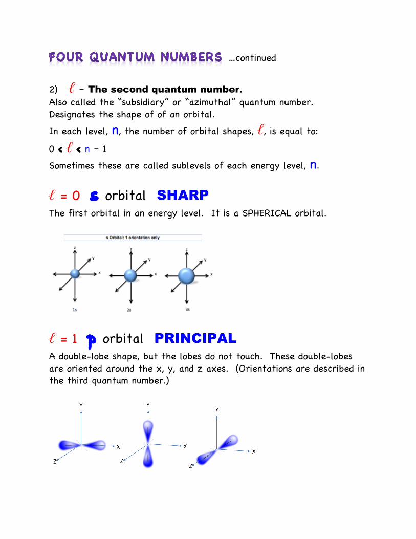
2) ℓ – The second quantum number. Also called the “subsidiary” or “azimuthal” quantum number. Designates the shape of of an orbital.

In each level, n, the number of orbital shapes, ℓ, is equal to: 0 < ℓ < n – 1

Sometimes these are called sublevels of each energy level, n.

ℓ = 0 s orbital SHARP The first orbital in an energy level. It is a SPHERICAL orbital.

   

ℓ = 1 p orbital PRINCIPAL A double-lobe shape, but the lobes do not touch. These double-lobes are oriented around the x, y, and z axes. (Orientations are described in the third quantum number.)

…continued

ℓ = 2 d orbital DIFFUSE

Complex lobe-shaped orbitals oriented around different axes in space.

ℓ = 3 f orbital FUNDAMENTAL VERY Complex lobe-shaped orbitals oriented around the different axes.

Please note that scientists have already started working on the probable electron distributions in g orbitals for elements from atomic number 121 and on, at ℓ = 4

…continued

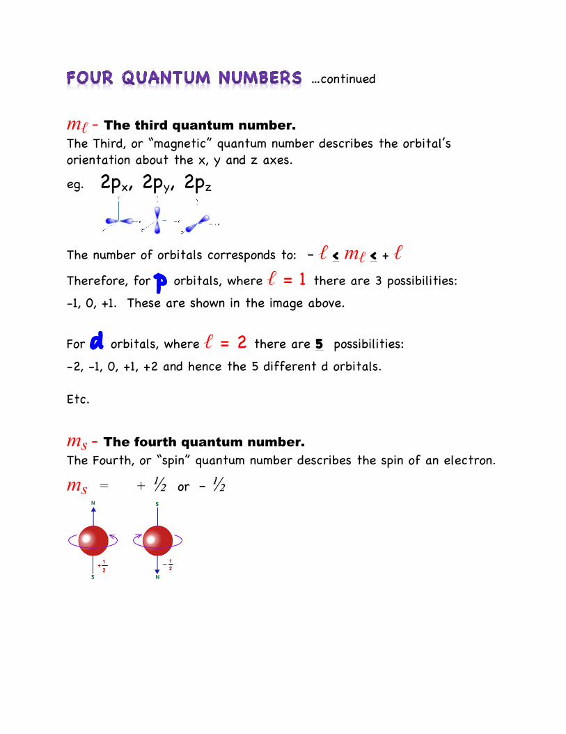
mℓ - The third quantum number. The Third, or “magnetic” quantum number describes the orbital’s orientation about the x, y and z axes.

eg. 2px, 2py, 2pz

The number of orbitals corresponds to: – ℓ < mℓ < + ℓ Therefore, for p orbitals, where ℓ = 1 there are 3 possibilities: -1, 0, +1. These are shown in the image above.

For d orbitals, where ℓ = 2 there are 5 possibilities:

-2, -1, 0, +1, +2 and hence the 5 different d orbitals. Etc.

ms - The fourth quantum number. The Fourth, or “spin” quantum number describes the spin of an electron.

ms = + ½ or – ½

SUMMARY – a closer look at the ℓ quantum number

On emission spectra (seen in the image above), the lines that show up on the film correspond to the s, p, d and f orbitals. These emission lines allow chemists to identify the element, based on the emission of energy from each of it’s electrons. s p d f

Number of orbitals of this shape

1 There is only one kind of s

orbital

3 There are 3 kinds of p orbitals

5 7

Maximum number of electrons per level (n)

2 In each s orbital, there can be 2 electrons (each with opposite spin)

6 In each of the

p orbitals, there can be 2 electrons (each with

opposite spin)

10 14

Describing  the  shape.  How many lobes does this shape have?

1

2

4

8

The Energy of electrons increase from s à pà d à f

Consider the element GALLIUM, atomic number 31. This neutral (uncharged) element has 31 electrons.

We NOW know that each of the electrons exist in complex three dimensional orbitals: Since Gallium is in the 4th row of the periodic table: n = 4 0 < ℓ < n – 1, so ℓ= 0, 1, 2, 3, meaning that orbitals represented by EACH of the l values, s, p, d, f, are possible . (But they may not all be filled by electrons!!!)

The mℓ and ms just tell us the orientations in space of the orbitals and the spin of the paired electrons so it is NOT necessary to look at these each time you write an electron configuration. NOTE:

The  complete  understanding  of  this  concept  will  occur  over  several  classes,  and  requires  you  to  practice,  daily,  until  you  reach  proficiency.      Reading  these  pages  is  not  enough  to  gain  a  full  understanding.      This  only  scratches  the  surface. In fact, the practice that we will do in class will put this into a more practical approach, rather than the mathematical approach as indicated by the quantum numbers, above.

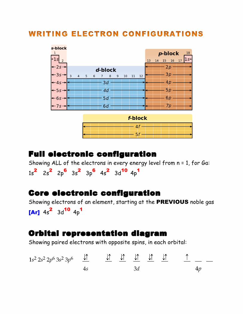
Full electronic configuration Showing ALL of the electrons in every energy level from n = 1, for Ga:

1s2 2s2 2p6 3s2 3p6 4s2 3d10 4p1

Core electronic configuration Showing electrons of an element, starting at the PREVIOUS noble gas

[Ar] 4s2 3d10 4p1

Orbital representation diagram Showing paired electrons with opposite spins, in each orbital:

Some textbooks, and even teacher worksheets, show full electron configurations as ENERGY DIAGRAMS, so that the energy differences of the electrons in each level is clearly demonstrated:

Practice done in class, with the teacher, on the white board, is essential for the understanding of electron configurations. We will start with basic FULL configurations, understanding the progression of the electron configurations from Hydrogen to Helium to Lithium, to Beryllium, etc. We will learn how to best distribute electrons in p orbitals so that we know when to have paired and unpaired electrons. As we enter the 3rd energy level, and d orbital electrons are possible, it is necessary to understand how to write the MOST STABLE electron configurations. And entering the 4th energy level, which introduces f orbital electron distributions, we must understand how an element would fill it’s orbitals in the proper energy level order. Practice in class will be accompanied by three dimensional images and videos on screen, as well has examples of emission spectra, so that you can understand this work that you are doing, IN CONTEXT. The sample questions will evolve organically, as we develop understanding of each aspect, so providing a full notes package on the practice questions would not be beneficial to your understanding, nor is it possible to predict each question in the order it will be presented. Once we are comfortable, we will also introduce ions, so that we understand WHERE an element would lose or gain electrons from, in order to achieve the most stable configuration. This will lead us into the ionic and covalent (molecular) bonding that we will be studying next. You will learn better by being able to work through this unit in consultation with your lab partners.