Remote Sensing of Environment 114 (2010) 1699–1709

Contents lists available at ScienceDirect

Remote Sensing of Environment

j ourna l homepage: www.e lsev ie r.com/ locate / rse

Development of a tundra-specific snow water equivalent retrieval algorithm forsatellite passive microwave data

C. Derksen a,⁎, P. Toose a, A. Rees b, L. Wang a, M. English b, A. Walker a, M. Sturm c

a Climate Research Division, Environment Canada, Toronto, Ontario, Canadab Department of Geography and Environmental Studies, Wilfrid Laurier University, Waterloo, Ontario, Canadac Cold Regions Research and Engineering Laboratory, U.S. Army Engineer Research and Development Center, Fort Wainwright, Alaska, United States

⁎ Corresponding author.E-mail address: Chris.Derksen@ec.gc.ca (C. Derksen)

0034-4257/$ – see front matter. Crown Copyright © 20doi:10.1016/j.rse.2010.02.019

a b s t r a c t

a r t i c l e i n f o

Article history:Received 25 November 2009Received in revised form 23 February 2010Accepted 26 February 2010

Keywords:Snow water equivalentPassive microwaveTundraSub-Arctic

Airborne and satellite brightness temperature (TB) measurements were combined with intensive fieldobservations of sub-Arctic tundra snow cover to develop the framework for a new tundra-specific passivemicrowave snow water equivalent (SWE) retrieval algorithm. The dense snowpack and high sub-grid lakefraction across the tundra mean that conventional brightness temperature difference approaches (such asthe commonly used 37 GHz–19 GHz) are not appropriate across the sub-Arctic. Airborne radiometermeasurements (with footprint dimensions of approximately 70×120 m) acquired across sub-Arctic Canadaduring three field campaigns during the 2008 winter season were utilized to illustrate a slope reversal in the37 GHz TB versus SWE relationship. Scattering by the tundra snowpack drives a negative relationship until athreshold SWE value is reached near 130 mm at which point emission from the snowpack creates a positivebut noisier relationship between 37 GHz TB and SWE.The change from snowpack scattering to emission was also evident in the temporal evolution of 37 GHz TBobserved from satellite measurements. AMSR-E brightness temperatures (2002/03–2006/07) consistentlyexhibited decreases through the winter before reaching a minimum in February or March, followed by anincrease for weeks or months before melt. The cumulative absolute change (Σ|Δ37V|) in vertically polarized37 GHz TB was computed at both monthly and pentad intervals from a January 1 start date and compared toground measured SWE from intensive and regional snow survey campaigns, and climate stationobservations. A greater (lower) cumulative change in |Δ37V| was significantly related to greater (lower)ground measured SWE (r2=0.77 with monthly averages; r2=0.67 with pentad averages). Σ|Δ37V| was onlyweakly correlated with lake fraction: monthly r2 values calculated for January through April 2003–2007 werelargely less than 0.2. These results indicate that this is a computationally straightforward and viablealgorithmic framework for producing tundra-specific SWE datasets from the complete satellite passivemicrowave record (1979 to present).

Crown Copyright © 2010 Published by Elsevier Inc. All rights reserved.

1. Introduction

A number of high priority science questions require snow waterequivalent (SWE) information across high latitude regions, including:

• determining whether there is an increase in high latitude winterseason precipitation to corroborate recent evidence from modelsimulations and the sparse network of conventional observations(Min et al., 2008; Zhang et al., 2007).

• identifying the role of snow cover variability and change in thepotential intensification of the high latitude water cycle throughincreased precipitation, earlier melt, higher peak runoff, and greaterfreshwater input to the Arctic Ocean (see Dery et al., 2009).

.

10 Published by Elsevier Inc. All rig

Conventional observations are not adequate to answer thesequestions because the station network is sparse and coastally biased,and the measurements themselves are uncertain. Snowfall gauge andshield combinations are not standard between countries (Yang et al.,1999), and the required auxiliary measurements for systematicundercatch correction (such as wind speed at gauge height) areoften not available. Point snow depth measurements are subject tolocal scale wind drifting or scour andmay not represent the prevailingregional conditions. Even when they do, the large distances betweenstations does not allow for meaningful spatial interpolation (i.e.kriging), and coastal stations do not represent vast inland areas.

Satellite passive microwave measurements address the spatiallimitations of conventional observations, but not necessarily theuncertainties in snow cover information. A large imaging footprint(25 km grid cell dimensions), wide swath, and general insensitivity tocloud cover produce spatially continuous daily brightness tempera-tures (TB) across latitudes north of approximately 60 °N. The response

hts reserved.

Table 1Summary of sub-Arctic in situ snow cover measurements.

Location Coordinates Time period Distance(km)

Measurements (n) SWE (mm)

Snow depth SWE Snowpits Mean Min Max SD

Puvirnituq, QC 59.83N–76.39W February 2008 18 ∼12,000 369 10 101 21 431 66Daring Lake, NT 64.85N–111.63W April 2008 33 ∼4400 668 23 100 3 428 64Trail Valley Creek, NT 68.70N–133.62W April 2008 28 ∼5900 757 27 111 15 534 61

1700 C. Derksen et al. / Remote Sensing of Environment 114 (2010) 1699–1709

of these TB measurements to seasonally evolving sub-Arctic snow andlake ice cover is poorly understood, however, and the performance ofhemispheric SWE retrieval algorithms (for example, Biancamariaet al., 2008; Chang et al., 1990; Kelly et al., 2003) across northernregions is not well documented due to the lack of high latitudemeasurements for algorithm validation. Algorithms developed forregional application across the boreal forest and open prairies do notperform well over the tundra (Derksen et al., 2005; Koenig & Forster,2004; Rees et al., 2006) because of the unique physical properties oftundra snow and the microwave contribution of the high fraction ofsub-grid lakes. The extreme variability of tundra snow on meter-to-meter length scales further complicates tundra algorithm develop-ment and validation at the scale of satellite microwavemeasurementsdue to the complexity in characterizing ‘ground-truth’ SWE.

Still, passive microwave retrievals remain an attractive option forsnow cover applications because of the theoretical relationshipbetween SWE and TB at 37 GHz (Matzler, 1994), and the considerablelength of the data record (1978–present). In this study, we present anew framework for a tundra-specific passive microwave SWEalgorithm developed through analysis of high resolution airbornepassive microwave measurements coupled with detailed in situ snowmeasurements from three field campaigns across sub-Arctic Canada,and satellite data from the Advanced Microwave Scanning Radiom-eter (AMSR-E). Specifically, we address two fundamental challengesto develop a tundra-specific SWE algorithm:

1. The unique radiometric properties of lake ice, which can constituteup to 40% of the sub-Arctic tundra land surface (primarily throughsmall sub-grid sized lakes). Derksen et al. (2009b) showed thatlake fraction is a primary control on tundra TB magnitude at allsatellite measured frequencies and thereforemust be considered aspart of a tundra specific retrieval scheme.

2. The slope reversal in the SWE versus 37 GHz Tb relationship, thatoccurs between 120 and 180 mmwater equivalent (Derksen, 2008;De Seve et al., 1997; Schanda et al., 1983). Below this threshold,increasing SWE is associated with lower TB due to volume scatter.Above this threshold, emission from the snowpack produces higherTB's with increasing SWE. Tundra snowpacks are typically shallow,dense, fine grained, and contain pronounced wind slab layers(Sturm et al., 1995). The influence of this stratigraphy on scatteringand emission behaviour can be complex, but there is documentedobservational evidence of the scattering to emission transitionduring late winter (Kim & England, 2003).

Accounting for these two factors is essential to avoid thesystematic SWE underestimation that is produced from contemporarybrightness temperature difference algorithms in tundra environments(Koenig & Forster, 2004; Rees et al., 2006).

2. Data

Interpreting TB response over tundra landscapes in winter requiresin situ observations of snow cover properties and lake ice character-istics. Optimally, these measurements would be available at contin-

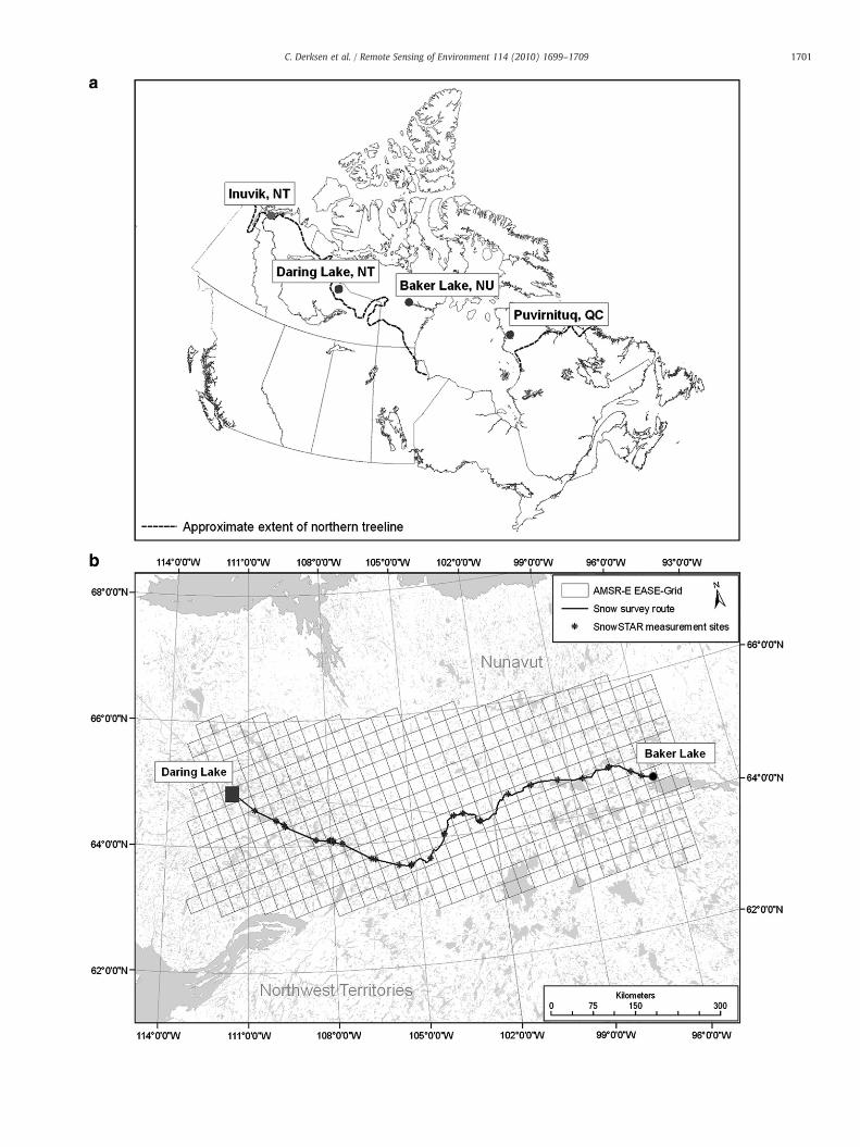
Fig. 1. (a) Study area overview showing the three IPY field campaign sites and the Baker Lakextent of AMSR-E EASE-Grid data used for analysis.

uous intervals through the season and adequately capture sub-gridvariability below the scale of satellite passive microwave measure-ments (25 km grid cell dimensions). In short, datasets with thesespatial and temporal characteristics are not available. In this study, weutilize datasets from a series of field campaigns conducted duringdiscrete time periods across the Canadian sub-Arctic tundra as part ofInternational Polar Year activities between February and April 2008.As summarized in Table 1, these campaigns included the deploymentof airborne passive microwave radiometers coupled with intensive insitu snow measurements. Collectively, these datasets provide theopportunity to determine relationships between snow cover proper-ties and microwave TB at multiple scales (airborne and satellite) frommultiple tundra sites. In turn, these relationships can be used todevelop the framework for a new tundra-specific SWE retrievalalgorithm that can be applied to the entire passivemicrowave satellitedata record that dates back to 1978.

2.1. Airborne radiometer measurements and in situ snow surveys

At all three tundra field sites (see Table 1; Fig. 1), airborne passivemicrowave measurements were acquired covering a wide range oftundra terrain. The radiometer installation (dual polarization 6.9, 19,37, and 89 GHz) on the National Research Council Twin Otter aircraftis described in MacPherson et al. (2001) andWalker et al. (2002). Theairborne radiometers (parameters for the 19 and 37 GHz radiometersused in this study are provided in Table 2) were calibrated pre- andpost each flight using warm (ambient temperature microwaveabsorber) and cold (liquid nitrogen) targets as described by Solheim(1993). Uncertainty in the measurement of the calibration targettemperature was estimated at+/-2 K. The 19 and 37 GHz radiometerswere calibrated simultaneously so the same target temperatureuncertainties for a given calibration apply to both frequencies.Estimates of inter-calibration receiver drift were made by examiningthe pre- and post-flight calibration target brightness temperatures.Radiometer stability was dependant on the frequency and variedsomewhat from campaign to campaign, but overall uncertainty wasestimated at +/−2 K at 19 GHz, and b1 K at 37 GHz.

Transects of snow depth and SWE measurements were acquiredalong segments of the radiometer flight lines, typically severalkilometers in length. Snow depth was sampled using a self recordingsnow depth probe (‘Magna Probe’ U.S. Patent No. 5864059; cf. Sturm& Liston, 2003) linked to a GPS. At all sites, manual SWE cores (usingan ESC-30 corer) were taken approximately every 250 m along thedepth transects, in order to compute bulk density values used toconvert the measured snow depth to estimated SWE. Average landcover specific snow densities were determined for each study site byrelating each ESC-30 measurement to a landscape class determinedfrom a Landsat classification (Natural Resources Canada, 2008). Theseland cover specific snow densities were used to estimate a SWE valuefor each snow depth measurement based on the land cover class itwasmeasured in. Density is an inherently conservative variable acrossthe tundra compared to snow depth, so this is an effective techniqueat converting a more straightforward measurement (depth) to a more

e climate station. (b) SnowSTAR snow survey route and measurement sites; grid shows

1701C. Derksen et al. / Remote Sensing of Environment 114 (2010) 1699–1709

Table 2Summary of radiometer characteristics.

Frequency

Frequency [GHz] 19 37Bandwidth [MHz] 1000 2000Integration time [s] 1.2 1.2Sensitivity [K] 0.04 0.03Accuracy [K] b2 b1θ3 dB [°] 6 6αi [°] 53 53Scan method Sideways along trackFlight altitude [m] 916Airspeed [m/s] 60Footprint size (w× l) 70×120 70×120

1702 C. Derksen et al. / Remote Sensing of Environment 114 (2010) 1699–1709

desirable variable (SWE; see Derksen et al., 2005). A summary of thein situ snow sampling transects is provided in Table 1.

Snowpits were also excavated at regular intervals along the flightlines. Stratigraphic observations including layer thickness were deter-mined by visual and physical examination of the snowpit face. Averagegrain size in each layerwas estimated frommanual observations using astereo-microscope and comparator card. Density profiles were deter-mined with 100cm3 cutters.

2.2. Satellite passive microwave measurements

AMSR-E TB's in both level 2 swath and EASE-Grid (Knowles et al.,2006) projections were acquired for October 1 through April 30, 2002to 2008. The use of the swath data is advantageous because theoriginal frequency dependant imaging characteristics are retained.Inter-orbit variability in swath level footprint locations, however,necessitated the use of the 25 km EASE-Grid dataset for the com-pilation of brightness temperature time series. A five-day movingaverage was applied to the descending orbit (approximately 0130local overpass time) AMSR-E data to reduce high frequency variabilityin TB driven by atmospheric and physical temperature effects (Markuset al., 2006).

2.3. Other snow measurements

To address regional snow information, data are available from acoordinated series of snowmeasurements made across the NorthwestTerritories and Nunavut, Canada in April 2007 during a snowmobiletraverse from Fairbanks, Alaska to Baker Lake, Nunavut (see Fig. 1b).Systematic snow measurements at the regional scale had not beenpreviously collected across this region of northern Canada. A fulldescription and analysis of the traverse measurements is provided inDerksen et al. (2009b). The most intensive period of samplingoccurred during the Daring Lake, Northwest Territories to BakerLake, Nunavut portion of the traverse (16 to 26 April, 2007). Samplesites were located at least every 1 °C of longitude. At these sites, snowdepth, density, snow water equivalent (SWE), stratigraphy, and grainsize measurements are available. Whenever possible, measurementswere made at paired sites: one on tundra (land) and one on ice (lakeor river ice depending on what was available) in order to capturemean regional SWE in this lake rich environment.

Temporally continuous snow observations are available fromclimate stations, but across the sub-Arctic tundra of Canada thesestations are extremely sparse and coastally biased. The only inlandobservations across the sub-Arctic Canadian tundra are from thecommunity of Baker Lake (64° 18′N 96° 4.8′ W; Fig. 1). Bi-weekly,manual observations of snow depth, density, and water equivalentmeasurements were acquired from the Environment Canada snowcourse at Baker Lake for algorithm development and validation.

3. Results

3.1. Radiometric measurements

Heterogeneity in land cover, terrain, vertical snowpack properties,and horizontal snow distribution are the reality within satellitepassive microwave measurements (25 km grid cell dimensions). Thisheterogeneity is also often unavoidable at airborne scales (even with80×100 m footprint dimensions) particularly in tundra environmentsdue to local scale snowpack variability. Given the analysis require-ment of linking groundmeasured SWE to airbornemeasured TB, it wasessential to accurately co-locate surface snow measurements withinthe airborne footprints to ensure a comparison covering the samephysical location on the ground.

ArcGIS™Geographic Information System(GIS) softwarewas used tolink surface snow measurements with airborne data by calculating theapproximate extent of the instantaneous field of view (IFOV) for eachairborne TB and then overlaying these airborne footprintswith the snowsurvey data to identify regions of overlap. The GPS Magna Probes geo-tag each snow depth observation with a latitude and longitudecoordinate. These units were WAAS enabled allowing for positionalaccuracy of better than 3 m 95% of the time (Garmin™, 2009; WAASsignal reception is ideal for open land and marine applications). Theairborne radiometer's IFOV is dependent on the aircraft's ground speedand altitude, as well as the radiometer's beamwidth, view angle, andintegration time. The radiometer's data acquisition system automati-cally calculates the latitude and longitude coordinates for each TB takinginto account the height above ground and the radiometer's beamwidthand view angle (based on the aircraft's pitch, roll and yaw).

The airborne radiometers had an integration time of approxi-mately 1.2 s. During this 1.2 s sampling sequence, there are 20 uniqueintegration cycles in which the radiometers measure emission in bothhorizontal and vertical polarization from the ground scene within theIFOV, as well as a noise diode and a load. Because of the forwardmomentum of the aircraft, the radiometer actually measures a slightlydifferent scene during each of the 20 integration cycles, each adjacentand overlapping one another, resulting in a larger IFOV in the along-track axis than what would be sampled from a stationary towermounted radiometer system. The 20 cycles are averaged together toproduce a single TB measurement for the entire IFOV. The radiometerintegration time is a fixed parameter and was not changed during theIPY field campaigns; however the aircraft speed did occasionally varybetween flights and during the same flight, but overall was quiteconsistent at approximately 110 nautical miles per hour (∼60 m/s,resulting in a typical IFOV size fluctuations in the along-track axis ofless than 10 m). These parameters resulted in a typical IFOV extent ofapproximately 80 m in the across-track axis and 100 m in the along-track axis. ArcGIS™ was used to create overlapping buffers, withvariable along-track axis lengths for each airborne TB measurement.These variable length buffers better represent the actual IFOV of theairborne radiometers, making it possible to determine which landcover characteristics and surface measurements were found withinthe footprint of each airborne radiometer.

Fig. 2 shows a visual representation of the snow survey and airbornedata collected during a short segment of data acquired near Puvirnituq,Quebec using ArcGIS™ software. The snow depth transect transitionsfromopen tundra on to a small pond and then back on to land. The blackdashed ellipses approximate the IFOV of the high resolution airborneradiometers (∼80 m×∼100 m). The two lines of points passing throughthe IFOVs represent two side-by-side snow depth transects, and eachindividual point is a snow depth measurement recorded using the GPSMagna Probes. The cross symbols represent the location of the manualESC-30 SWE measurements recorded to obtain the bulk snowpackdensity and SWE.

In reality, the precise co-location of surface snow measurementswithin an airborne TB footprint does not always occur due to errors in

Fig. 2. Approach of linking the transect snowmeasurements to the airborne footprints. Large ellipses illustrate airborne microwave footprints, red circles indicate Magna Probe snowdepths, and yellow crosses indicate ESC-30 snow cores used to convert depth measurements to SWE.

1703C. Derksen et al. / Remote Sensing of Environment 114 (2010) 1699–1709

the aircraft flight path and/or the ground location of the snowsurveyors. In total 995 TB's from all three trans-tundra study sitelocations had 11,909 coincident SWEmeasurements within the IFOV'sof the radiometers. However, this includes microwave footprintswhich potentially only had a single snow measurement and/or hadmeasurements at the very edge of an IFOV boundary. Therefore, toensure that each TB was compared to an adequate and representativenumber of SWE measurements a simple filtering process was used.The first stage of filtering eliminated all TB's with snowmeasurementsat the margins of the IFOV that might not have been representative ofthe snowpack within the IFOV itself. This was accomplished by usingArcGIS™ software to select only those TB's with snow measurementsat least 10 m inside the boundary of the IFOV, resulting in a total of803 TB's with 9253 coincident SWE measurements.

The second step of the filtering process involved selecting onlythose TB's with a large enough number of snow measurements tocapture the local scale variability in SWE that is common for theheterogeneous tundra snowpack. Therefore, only those airborne TB'swith at least 10 SWE measurements within the IFOV were selectedfor this analysis. A sample size of at least 10 snow measurementswas considered large enough to not be overly affected by one or twonon-representative measurements within the IFOV. This selectionprocess resulted in a total of 714 TB's with 9028 coincident SWEmeasurements.

The expected TB response at 37 GHz to a range of SWE between 0and 600 mm is shown in Fig. 3a (modified from Matzler et al., 1982).Two distinct slopes are evident: a negative relationship driven bysnowpack volume scatter, and a positive relationship driven by

snowpack emission. The slope reversal in this relationship (atapproximately 150 mm in the case of these data) illustrates theSWE ‘saturation’ problem with empirical brightness temperaturedifference algorithms that rely on 37 GHz measurements: the same TBdifference is associated with two SWE estimates that can differ byover 200 mm.With the full range of SWE encountered across all threeof the field campaigns (as summarized in Table 1), we sought toreproduce the relationship in Fig. 3a with our much larger IPY fielddataset. A comparison of in situ measured SWE and 37V TB from the714 airborne measurements retained as described above is shown inFig. 3b.

The field observations do capture the same slope reversalphenomenon, albeit with some noise (both relationships identifiedin Fig. 3b are statistically significant at 99%). The scattering influenceof the snowpack is evident only to a threshold just below 130 mmafter which increasing SWE is coincident with an increase in 37 GHzTB due to snowpack emission. This threshold is slightly lower thanreported in some studies (i.e. De Seve et al., 1997; Matzler, 1994) butvery similar to direct measurements (with ground based microwaveradiometers) of the transition of a tundra snowpack from volumescatter to emission provided in Sturm et al. (1993). Their measure-ments identified volume scatter to a critical snow depth of 31 cm;depths above this threshold produced an increase in the effectiveemissivity at 37 GHz. These measurements were made by removinglayers from the snowpack near the end of the accumulation season, asopposed to measuring the natural accumulation and metamorphosisof the snowpack. Regardless, presuming a basal depth hoar layerdensity of 350 kg m−3, the SWE at the 31 cm threshold in the Sturm et

Fig. 3. (a) Expected relationships between 37 GHz TB and SWE (adapted from Matzler et al., 1982); (b) airborne TB versus in situ SWE from all three field campaigns; (c) monthlyaveraged 36.5 GHz (V-pol) AMSR-E TB's from 2004/05 for the domain in Fig. 1b.

1704 C. Derksen et al. / Remote Sensing of Environment 114 (2010) 1699–1709

al. (1993) measurements was approximately 110 mm, close to the130 mm scattering to emission inflection identified with the airbornedata in Fig. 3b.

The degree of noise in the ground measured SWE versus airborneTB relationship was anticipated given the inherent uncertainty in theability of the field observations to accurately characterize meanfootprint SWE. The challenge of acquiring snow cover measurementtransects within a 100 m wide airborne measurement swath acrossthe tundra should not be underestimated. In addition, variabilitydriven by factors such as underlying vegetation properties andsnowpack properties such as depth hoar layer thickness were notconsidered. A detailed comparison of vertical snowpack propertiesand measured TB was addressed by Rees et al. (2010).

An important scaling question is whether the expected TB versusSWE slope reversal (Fig. 3a) captured by the airborne measurements(Fig. 3b) was also observed at the satellite scale. Snow coursemeasurements from Baker Lake were compared to five-day (pentad)averaged AMSR-E 37 GHz TB's from the EASE-Grid cell in which thesnow course is located (Fig. 3c) over the 2002 to 2008 time period. Thetransition from snowpack scatter to emission at 37 GHz is evident atthe satellite scale, but with a TB minima near 70 mm SWE, followed byincreased TB with higher SWE. While the slope reversal is thereforeevident at both airborne and satellite scales, the inflection point in theTB versus SWE relationship occurs at a much lower SWE threshold atthe satellite scale than would be expected given the ground based andairborne radiometer results in Fig. 3a and b. The difference betweenthe airborne and satellite inflection points is likely related to scaleissues. Unlike the relatively homogeneous airborne measurements,the AMSR-E footprint that covers Baker Lake is composed ofapproximately 30% lake fraction. This sub-grid heterogeneity willhave a seasonally evolving influence on TB throughout the winter thatdoes not influence the airborne data. In addition, the Baker Lake snowcourse covers a relatively localized area, which may underestimatethe surrounding tundra SWE.

3.2. Tundra-specific algorithm concept

The multi-scale behaviour of 37 GHz TB's over snow coveredtundra illustrated in Fig. 3 led to the development of a singlefrequency solution for tundra SWE retrievals based solely on verticallypolarized 37 GHz measurements. The primary advantages of thissingle frequency approach for tundra regions are:

1. 37 GHzmeasurements exhibit consistent correlation with lake fractionacross the sub-Arctic tundra from January onwards (Derksen et al.,

Fig. 4. Boxplots of monthly averaged AMSR-E 36.5 GHz TB (left column) and cumulative absol07 (bottom).

2009b). While low frequency measurements (6.9; 10.7 GHz) arecontrolled by emission from below the ice layer through the entirewinter season, higher frequency measurements including thosecommonly used to retrieve SWE (∼19 and 37 GHz) havepenetration depths that are strongly influenced by water beneaththe ice for part of the season, but are also influenced by the ice andoverlying snowpack by the end of the season. The timing of thisshift in the primary emission source is different at 19 versus37 GHz, so the traditional brightness temperature differenceapproach (37 GHz–19 GHz) is not appropriate for lake rich tundraenvironments. By January, the combined thickness of lake ice andsnow cover exceeds the 37 GHz penetration depth, and so issufficient to mask the liquid water signal beneath the ice, creatingconsistent correlations with lake fraction through the remainder ofthe snow cover season.

2. Unlike complications that can arise across the boreal forest (seeDerksen, 2008; De Roo et al., 2007), vegetation influences on 37 GHzTb's are minimal across the tundra.

3. Vertical polarization 37 GHz measurements exhibit low sensitivity(compared to horizontal polarization measurements) to verticalsnowpack structure, including ice lenses (Derksen et al., 2009b;Rees et al., 2010).

The primary challenge with a single frequency approach, however,is the fact that multiple values of SWE are related to the same TB asillustrated in Fig. 3 and discussed in the previous section. To addressthis, the month to month cumulative absolute change for verticallypolarized 37 GHz TB (Σ|Δ37V|) was calculated on a grid cell by grid cellbasis for the seasons spanning 2002/03 through 2006/07. Boxplotswere produced that show both the monthly averaged 37 GHz TB andthe absolute cumulative change in 37 GHz TB (Fig. 4).

The use of absolute change at 37 GHz accounts for the decrease inTB during the first portion of the winter season (primary mechan-ism=snowpack scatter), and the subsequent increase in TB as SWEexceeds a critical threshold (primary mechanism=snowpack emis-sion). The hypothesis is that any change in TB observed during theJanuary through April period in the tundra environment is largely dueto an increase in SWE. Therefore, the greater (lower) the cumulativechange in 37 GHz TB calculated between January and April, the greater(lower) the SWE. During heavy snow years, the minimum TBcorresponding to the SWE threshold is reached early, and increasesin SWE act to increase TB's resulting in higher absolute cumulativechange in 37 GHz TB. During light snow years, the minimum TBcorresponding to the 100 mm SWE threshold is reached later or notat all, and continued changes in TB are minimal resulting in lower

ute change (Σ|Δ37V|) over the domain shown in Fig. 1b for 2002/03 (top) through 2006/

1705C. Derksen et al. / Remote Sensing of Environment 114 (2010) 1699–1709

1706 C. Derksen et al. / Remote Sensing of Environment 114 (2010) 1699–1709

cumulative change in 37 GHz TB. A source of uncertainty will be TBchanges associated with snow metamorphism and not changes inSWE. A quantitative examination of this issue depends on seasonallycontinuous physical snowpack observations coupled with highresolution TB measurements; field experiments during the 2009/10winter in support of the The COld REgions Hydrology High-resolutionObservatory (CoRe-H2O; Rott et al., 2008) will provide thisopportunity.

We would expect the single frequency change in 37 GHz to beinsensitive to lake fraction from January onwards based on thecorrelation results between TB and lake fraction presented in Derksenet al. (2009b). To confirm this assumption, correlation analysis wasperformed on monthly averaged change |Δ37V| TB (calculated fromthe EASE-Grid AMSR-E brightness temperatures) and lake fraction(produced by the U.S. Geological Survey and re-gridded to the EASE-Grid). Five winter seasons (January through April; 2002/03–2006/07)of AMSR-E data were analyzed, producing five correlation values foreach month. Boxplots of these correlation values over the five yearsare shown in Fig. 5, with the relationships betweenmonthly |Δ37V| TBand lake fraction interannually consistent and weak.

3.3. Prototype algorithm and evaluation

AMSR-E data, averaged over monthly periods to remove highfrequency noise, were initially used to investigate relationshipsbetween cumulative absolute change in 37 GHz TB and SWE. Fivewinter seasons (2002/03–2006/07) were investigated. On a grid cellby grid cell basis, mean monthly 37V TB was calculated for Decemberthrough April. The absolute month to month change in 37V was thencalculated:

Δ37Vmonth i = j37Vmonth i−37Vmonth i−1j ð1Þ

This step produces an absolute Δ37V term for each month, Januarythrough April. These values were then summed (Σ|Δ37V|) for eachEASE-Grid cell in a cumulative fashion from month to month throughthe season. For example, the value forMarch is the sum of themonthlychange in absolute 37V TB from December to January, January toFebruary, and February to March. This process shifts the seasonal U-shaped evolution of 37V TB (as illustrated in Fig. 3 and the left columnof Fig. 4) to an approximately linear seasonal evolution (as illustratedin the right column of Fig. 4).

To account for variability in December 37V TB caused by a variety offactors including early season snow accumulation, lake ice thickness,and physical temperature, the starting point for the calculation ofEq. (1) for Januarywas determined by calculating the 37V TB difference

Fig. 5. Box plots of correlation between monthly averaged change in 37 GHz TB and lakefraction, 2002/03–2007/08, for the domain shown in Fig. 1. Shading denotesinsignificant correlations at 95%.

for each individual December relative to the monthly mean over thefull AMSR-E period of record (2002–2008). For example, the startingpoint for the 2002/03 calculations is shown in Eq. (2).

37VSTART = 37VDec2002�−37V

Dec2002−2008�

:ð2Þ

This value can be either positive or negative. For January, Δ37V iscalculated as:

Δ37VJan = j37VSTART−37VJanj: ð3Þ

For each subsequent month, it follows Eq. (1).The monthly Δ37V values were then compared to tundra SWE

datasets derived from surface measurements taken from threesources:

1. Environment Canada snow course measurements from Baker Lake(see Fig. 1a) available bi-weekly for all six seasons.

2. Mean SWE for an AMSR-E grid cell covering the Daring Lake studyarea (see Fig. 1b), determined from a terrain weighted average ofall in situ SWE measurements acquired during field campaigns inApril between 2003 and 2008.

3. Regional SWE measurements acquired between Daring Lake andBaker Lake during the April 2007 SnowSTAR traverse (see Fig. 1b)described in Derksen et al. (2009b).

Results of this assessmentwere very encouragingwhen the datasetswere compared at amonthly time step (r2=0.77; significant at 95%), asillustrated in Fig. 6a. Themeasured SWEvalues cover a reasonable rangein SWE, encompass different snowpack ages (thin tundra snow inJanuary; a mature multi-layer snowpack near peak SWE in April) andlake rich and lake poor areas. The analysis was repeated at the pentad(five-day) average time step to see if the monthly results were trans-ferable to a finer temporal scale. All calculations follow Eqs. (1)–(3), but

Fig. 6. Relationship between AMSR-E cumulative Δ37V and ground measured SWE atmonthly (a) and pentad (b) time steps.

1707C. Derksen et al. / Remote Sensing of Environment 114 (2010) 1699–1709

with monthly TB data replaced with pentad data. Pentad averages werecalculated from 1 January through 30 April (24 pentads). These valueswere then summed (Σ|Δ37V|) for each pixel in a cumulative fashionfrom pentad to pentad through the season. For example, by 30 Januaryyou have summed 6 pentads; by 30 April you have summed 24 pentads.As in Eq. (3), the starting point for the calculation of Eq. (1) for pentad01(January 1 to 5) is determined by computing the 37V Decemberdifference as defined previously. The pentad resolution relationshipbetweenΣ|Δ37V| and SWE is shown in Fig. 6b.While somewhatweakerthan the monthly average results, a significant relationship (r2=0.67;significant at 95%) is still evident.

3.4. Comparison with a previous algorithm

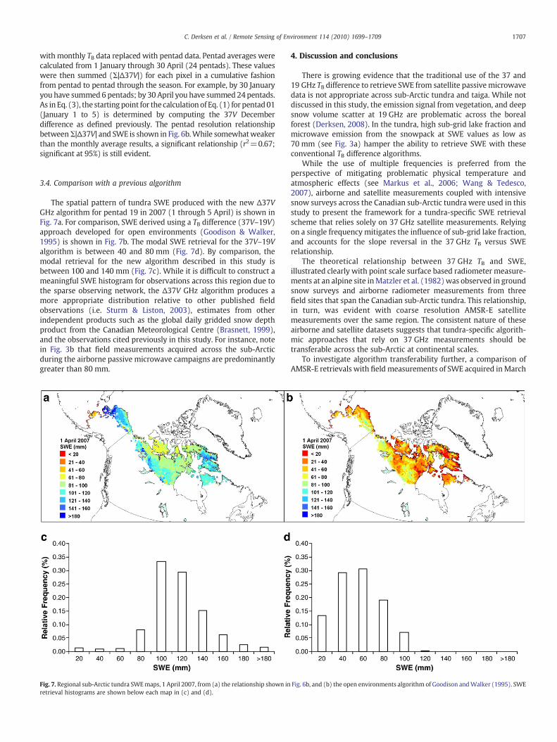
The spatial pattern of tundra SWE produced with the new Δ37VGHz algorithm for pentad 19 in 2007 (1 through 5 April) is shown inFig. 7a. For comparison, SWE derived using a TB difference (37V–19V)approach developed for open environments (Goodison & Walker,1995) is shown in Fig. 7b. The modal SWE retrieval for the 37V–19Valgorithm is between 40 and 80 mm (Fig. 7d). By comparison, themodal retrieval for the new algorithm described in this study isbetween 100 and 140 mm (Fig. 7c). While it is difficult to construct ameaningful SWE histogram for observations across this region due tothe sparse observing network, the Δ37V GHz algorithm produces amore appropriate distribution relative to other published fieldobservations (i.e. Sturm & Liston, 2003), estimates from otherindependent products such as the global daily gridded snow depthproduct from the Canadian Meteorological Centre (Brasnett, 1999),and the observations cited previously in this study. For instance, notein Fig. 3b that field measurements acquired across the sub-Arcticduring the airborne passive microwave campaigns are predominantlygreater than 80 mm.

Fig. 7. Regional sub-Arctic tundra SWEmaps, 1 April 2007, from (a) the relationship shown inretrieval histograms are shown below each map in (c) and (d).

4. Discussion and conclusions

There is growing evidence that the traditional use of the 37 and19 GHz TB difference to retrieve SWE from satellite passivemicrowavedata is not appropriate across sub-Arctic tundra and taiga. While notdiscussed in this study, the emission signal from vegetation, and deepsnow volume scatter at 19 GHz are problematic across the borealforest (Derksen, 2008). In the tundra, high sub-grid lake fraction andmicrowave emission from the snowpack at SWE values as low as70 mm (see Fig. 3a) hamper the ability to retrieve SWE with theseconventional TB difference algorithms.

While the use of multiple frequencies is preferred from theperspective of mitigating problematic physical temperature andatmospheric effects (see Markus et al., 2006; Wang & Tedesco,2007), airborne and satellite measurements coupled with intensivesnow surveys across the Canadian sub-Arctic tundra were used in thisstudy to present the framework for a tundra-specific SWE retrievalscheme that relies solely on 37 GHz satellite measurements. Relyingon a single frequency mitigates the influence of sub-grid lake fraction,and accounts for the slope reversal in the 37 GHz TB versus SWErelationship.

The theoretical relationship between 37 GHz TB and SWE,illustrated clearly with point scale surface based radiometer measure-ments at an alpine site inMatzler et al. (1982)was observed in groundsnow surveys and airborne radiometer measurements from threefield sites that span the Canadian sub-Arctic tundra. This relationship,in turn, was evident with coarse resolution AMSR-E satellitemeasurements over the same region. The consistent nature of theseairborne and satellite datasets suggests that tundra-specific algorith-mic approaches that rely on 37 GHz measurements should betransferable across the sub-Arctic at continental scales.

To investigate algorithm transferability further, a comparison ofAMSR-E retrievals with field measurements of SWE acquired inMarch

Fig. 6b, and (b) the open environments algorithm of Goodison andWalker (1995). SWE

Table 3Comparison of algorithm performance assessed with Alaskan north slope measure-ments from Sturm and Liston (2003).

Year Dates Mean SWE(mm)

37V–19V 37V

RMSE Mean bias RMSE Mean bias

2007 29 March–2 April 100 49 −45 22 52008 20–24 April 84 29 −12 39 37

1708 C. Derksen et al. / Remote Sensing of Environment 114 (2010) 1699–1709

2000 and April 2002 from the north slope of Alaska (described inSturm & Liston, 2003) is summarized in Table 3. Significant under-estimation with a TB difference algorithm (37V–19V) is apparent forboth years, consistent with the results of Koenig and Forster (2004).Retrievals with the new Δ37V GHz algorithm agree strongly with thefield measurements from 2000 with an RMSE of 22 mm and a meanbias of −5 mm. In 2002, when the field measurements were maderelatively late in the season (April 20 to 24), the results highlight achallenge with the new 37 GHz single frequency approach. Late in thewinter, large changes in TB can occur over short time periods as thesnowpack begins tomelt and refreeze. Because the SWE retrievals willcontinue to increase as TB's evolve through the season, these diurnalchanges create an overestimation of SWE, as illustrated by the highpositive bias with the new algorithm (Table 3). It will be necessary toidentify an end date after which large TB fluctuations make the SWEretrievals unreliable. This should be relatively straightforwardthrough the use of melt onset detection algorithms available forQuikSCAT (Wang et al., 2008) and passive microwave data (Takalaet al., 2009).

The next phase in this work is to examine the data record prior toAMSR-E, and apply this prototype algorithm to Scanning Multichan-nel Microwave Radiometer (SMMR; 1978–1987) and Special SensorMicrowave/Imager (SSM/I) measurements. Because only a singlefrequency is utilized, ensuring inter-sensor TB homogeneity will berelatively straightforward. This 30 year data record will characterizevariability in SWE across the tundra, and address priority researchissues that are difficult to answer with sparse conventional observa-tions. Analysis of snow extent and snow cover duration from theNOAA snow chart record (1966–present) shows a decrease in thelength of the Arctic snow cover season, driven by earlier spring snowmelt (Derksen et al., 2009a). Linking trends in SWE from the satellitepassive microwave record with snow extent and melt timing (forexample, Wang et al., 2008) datasets will contribute to characterizingthe role of terrestrial snow cover in the high latitude water cycle overthe past three decades.

Acknowledgments

Thanks to Ken Asmus, Walter Strapp and Arvids Silis ofEnvironment Canada for support with radiometer measurementsand field activities. AMSR-E brightness temperatures were acquiredfrom the National Snow and Ice Data Center, Boulder, Colorado. Fieldactivities during 2008 near Puvirnituq, Daring Lake, and Inuvik weresupported by the Government of Canada International Polar Yearfunding to the ‘Variability and Change in the Canadian Cryospere’network project. SnowSTAR 2007 was supported by the NationalScience Foundation, the Cold Regions Research and EngineeringLaboratory, and Environment Canada. Field measurements at DaringLake prior to 2008 were supported by the Canadian Foundation forClimate and Atmospheric Science.

References

Biancamaria, S., Mognard, N., Boone, A., Grippa, M., & Josberger, E. (2008). A satellitesnow depth multi-year average derived from SSM/I for the high latitude regions.Remote Sensing of Environment, 112, 2557−2568.

Brasnett, B. (1999). A global analysis of snow depth for numerical weather prediction.Journal of Applied Meteorology, 38, 726−740.

Chang, A., Foster, J., & Hall, D. (1990). Satellite sensor estimates of northern hemispheresnow volume. International Journal of Remote Sensing, 11(1), 167−171.

Derksen, C. (2008). The contribution of AMSR-E 18.7 and 10.7 GHz measurementsto improved boreal forest snow water equivalent retrievals. Remote Sensing ofEnvironment, 112, 2700−2709.

Derksen, C., Brown, R., & Wang, L. (2009). Terrestrial snow (Arctic). State of the Climatein 2008. Bulletin of the American Meteorological Society, 90. (pp. S1−S196).

Derksen, C., Sturm, M., Liston, G., Holmgren, J., Huntington, H., Silis, A., et al. (2009).Northwest Territories and Nunavut snow characteristics from a sub-Arctic traverse:Implications for passivemicrowave remote sensing. Journal of Hydrometeorology, 10(2), 448−463.

Derksen, C., Walker, A., & Goodison, B. (2005). Evaluation of passive microwave snowwater equivalent retrievals across the boreal forest/tundra transition of westernCanada. Remote Sensing of Environment, 96(3/4), 315−327.

De Roo, R., Chang, A., & England, A. (2007). Radiobrightness at 6.7-, 19-, and 37-GHzdownwelling from mature evergreen trees observed during the Cold LandProcesses Experiment in Colorado. IEEE Transactions on Geoscience and RemoteSensing, 45(10), 3224−3229.

Dery, S., Hernandez-Henrıquez, M., Burford, J., & Wood, E. (2009). Observationalevidence of an intensifying hydrological cycle in northern Canada. GeophysicalResearch Letters, 36, L13402. doi:10.1029/2009GL038852.

De Seve, D., Bernier, M., Fortin, J. -P., & Walker, A. (1997). Preliminary analysis of snowmicrowave radiometry using the SSM/I passive-microwave data: The case of LaGrande River watershed (Quebec). Annals of Glaciology, 25, 353−361.

Garmin™, 2009. About GPS—What is WAAS? Available at: http://www8.garmin.com/aboutGPS/waas.html [Accessed July 29th 2009]

Goodison, B., & Walker, A. (1995). Canadian development and use of snow coverinformation from passive microwave satellite data. In B. Choudhury, Y. Kerr, E.Njoku, & P. Pampaloni (Eds.), PassiveMicrowave Remote Sensing of Land–AtmosphereInteractions (pp. 245−262). Utrecht, Netherlands: VSP BV.

Kelly, R., Chang, A., Tsang, L., & Foster, J. (2003). A prototype AMSR-E global snow areaand snow depth algorithm. IEEE Transactions on Geoscience and Remote Sensing, 41(2), 230−242.

Kim, E., & England, A. (2003). A yearlong comparison of plot-scale and satellite footprint-scale 19 and 37 GHz brightness temperature of the Alaskan North Slope. Journal ofGeophysical Research, 108(D13), 4388−4403. doi:10.1029/2002JD002393.

Knowles, K., Savoie, M., Armstrong, R., Brodzik, M. J. (2006, updated 2008). AMSR-E/Aqua daily EASE-Grid brightness temperatures, 2003–2008. Boulder, ColoradoUSA: National Snow and Ice Data Center. Digital media.

Koenig, L., & Forster, R. (2004). Evaluation of passive microwave snowwater equivalentalgorithms in the depth hoar-dominated snowpack of the Kuparuk Riverwatershed, Alaska, USA. Remote Sensing of Environment, 93, 511−527.

MacPherson, I., Marcotte, D., & Jordan, J. (2001). The NRC atmospheric research aircraft.Canadian Aeronautics and Space Journal, 47(3), 1−11.

Markus, T., Powell, D., & Wang, J. (2006). Sensitivity of passive microwave snow depthretrievals to weather effects and snow evolution. IEEE Transactions on Geoscienceand Remote Sensing, 44(1), 68−77.

Matzler, C. (1994). Passive microwave signatures of landscapes in winter. Meteorologyand Atmospheric Physics, 54, 241−260.

Matzler, C., Schanda, E., & Good, W. (1982). Towards the definition of optimum sensorspecifications for microwave remote sensing of snow. IEEE Transactions on Geoscienceand Remote Sensing, GE-20, 57−66.

Min, S. -K., Zhang, X., & Zwiers, F. (2008). Human-induced Arctic moistening. Science,320, 518−520.

Natural Resources Canada. (2008). Circa-2000 Northern Land Cover of Canada. [DigitalRaster Data]. 2008.Ottawa, Ontario: Canada Centre for Remote Sensing, GeoAccessDivision Available at: http://geogratis.cgdi.gc.ca/download/landsat_7/Northern_-Land_Cover [Accessed June 2008].

Rees, A., Derksen, C., English, M., Walker, A., & Duguay, C. (2006). Uncertainty in snowmass retrievals from satellite passive microwave data in lake-rich high-latitudeenvironments. Hydrological Processes, 20, 1019−1022.

Rees, A., Lemmetyinen, J., Derksen, C., Pulliainen, J., & English, M. (2010). Observed andmodelled effects of ice lens formation on passive microwave brightness tempera-tures over snow covered tundra. Remote Sensing of Environment, 114, 116−126.

Rott, H., Cline, D., Duguay, C., Essery, R., Haas, C., Kern, M., et al. (2008). Scientificpreparations for CoReH20, a dual frequency SAR mission for snow and iceobservations. CD-ROM Proceedings, 2008 International Geoscience and Remote SensingSymposium, Boston MA.

Schanda, E., Matzler, C., & Kunzi, K. (1983). Microwave remote sensing of snow cover.International Journal of Remote Sensing, 4(1), 149−158.

Solheim, F. (1993). Use of pointed water vapor radiometer observations to improvevertical GPS surveying accuracy. Unpublished Ph.D. Dissertation, Dept. Physics,Univ. Colorado, Boulder.

Sturm, M., Grenfell, T., & Perovich, D. (1993). Passive microwavemeasurements of taigaand tundra snow covers in Alaska, U.S.A.. Annals of Glaciology, 17, 125−130.

Sturm, M., Holmgren, J., & Liston, G. (1995). A seasonal snow cover classification systemfor local to global applications. Journal of Climate, 8, 1261−1283.

Sturm, M., & Liston, G. (2003). Snow cover on lakes of the Arctic Coastal Plain of Alaska,U.S.A. Journal of Glaciology, 49(166), 370−380.

Takala, M., Pulliainen, J., Metsamaki, S., & Koskinen, J. (2009). Detection of snowmeltusing spaceborne microwave radiometer data in Eurasia from 1979 to 2007. IEEETransactions on Geoscience and Remote Sensing, 47(9), 2996−3007.

Walker, A., Strapp, J. W., & MacPherson, I. (2002). A Canadian Twin Otter microwaveradiometer installation for airborne remote sensing of snow, ice and soil moisture.

1709C. Derksen et al. / Remote Sensing of Environment 114 (2010) 1699–1709

CD-ROM Proceedings, International Geoscience and Remote Sensing Symposium,Toronto, June, 2002.

Wang, L., Derksen, C., & Brown, R. (2008). Detection of Pan-Arctic TerrestrialSnowmelt from QuikSCAT, 2000–2005. Remote Sensing of Environment, 112(10),3794−3805.

Wang, J., & Tedesco, M. (2007). Identification of atmospheric influences on theestimation of snow water equivalent from AMSR-E measurements. Remote Sensingof Environment, 111, 398−408.

Yang, D., Goodison, B., Metcalfe, J., Louie, P., Leavesley, G., Emerson, D., et al. (1999).Quantification of precipitationmeasurement discontinuity induced bywind shieldson national gauges. Water Resources Research, 35(2), 491−508.

Zhang, X., Zwiers, F., Hegerl, G., Lambert, H., Gillett, N., Solomon, S., et al. (2007).Detection of human influence on twentieth-century precipitation trends. Nature,448, 461−465.