PUSAN NATIONAL UNIVERSITY

Deriving Situation-Adaptive Strategy for Stacking

Containers in an Automated Container Terminal

Taekwang Kim, Jeongmin Kim, and Kwang Ryel Ryu

Pusan National University

Dept. of Electrical and Computer Engineering

0

Outline

• Automated Container terminal

• Stacking Policy

• Background and Previous Works

• Approach to Deriving Situation-Adaptive Strategy

• Case Study

• Experimental Results

• Conclusion

1

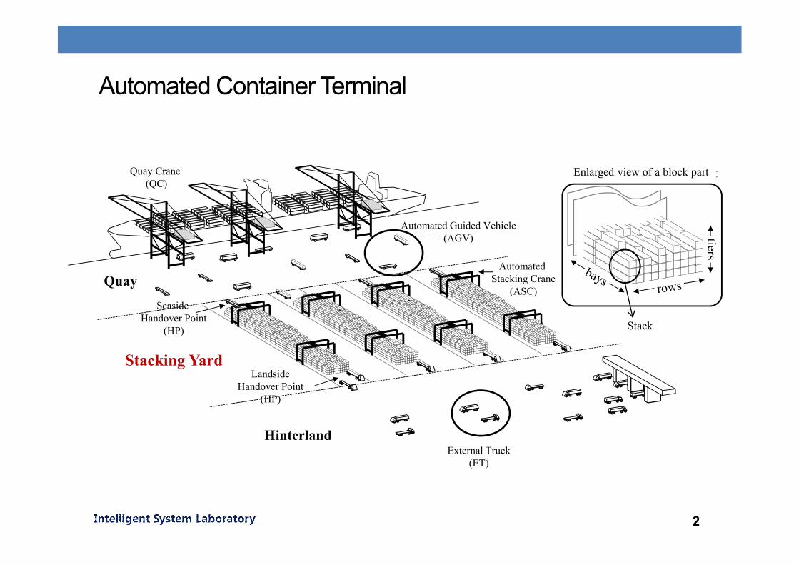
Automated Container Terminal

2

Enlarged view of a block part

tiers

Seaside

StackingYard

LandsideExternalTrucks

AGVs

QC

Seaside ASC

Seaside HP

Landside HP

Landside ASC

Quay

Quay Crane (QC)

Hinterland

Enlarged view of a block part

Stacking Yard

External Truck(ET)

Automated Stacking Crane

(ASC)

Automated Guided Vehicle(AGV)

Seaside Handover Point

(HP)

LandsideHandover Point

(HP)

Stack

Operations in Stacking Yard

• Crane interference occurs frequently because of the opposite

directions of container flow

• Determination of stacking position is one of the most important

operational problems in container terminals

3

Seaside HP

Landside HP

Loading Carry-in(Export)

Carry-outRehandling

Transshipment

Discharging(Import)

Repositioning

Stacking Policy

• Stacking policy takes account of various criteria to determine optimal

stacking positions in the stacking yards

• A good position should allow efficient operation not only at the time of

stacking but also at the time of retrieval

4

Stacking Policy

container 1. Request for a stacking location

3. An optimal stacking position

4. Stack

Stacking yard

2. Evaluate candidate positions

• Stacking policy based on single criterion [Duinkerken M. B., 2001]

[Dekker, R., 2006]

Background and Previous Works

5

Distance to the Handover Point

Category of a container (destination, weight, type)

Container type

(e.g. normal, reefer, dangerous goods)

Maximum stack height

Constraints

Background and Previous Works

• Stacking policy based on multiple criteria [Park, T., 2010a] [Park, T.,

2010b]

• Multiple criteria are taken into account simultaneously by a scoring function

of a weighted sum

x a candidate position

Ci i-th criterion

wi weight for the i-th criterion

• The position with the best score is selected

• Stacking policy is represented as a vector of the weight values

6

( ) ( )i ii

s x w C x

Background and Previous Works

• Stacking policy based on multiple criteria

• A policy consists of a set of rules for various container types

7

Background and Previous Works

8

• Stacking policy based on multiple criteria

Example: s7 (R7) for repositioning export containers

s7(x) = w34DI(x) + w35DO(x) + w36H(x) + w37E(x) + w38T(x) + w39G(x) + w40S(x)

DI(x)The distance in number of bays from the current location of the target container to the candidate location x

DO(x) The distance from x to a seaside HP of the block

H(x) The height of the stack at x

E(x)Indicates whether or not the candidate location is an empty ground slot

T(x)Indicates whether or not the container at the top of the stack at xis a repositioned container

G(x)The estimated likelihood of causing rehandling if the target container is eventually put on x

S(x)The amount of reduction in empty ground slots after putting the target container on x

• Deriving a robust stacking policy using a Noise-Tolerant Genetic

Algorithm (NTGA) [Jang, H., 2012]

• An evaluation of a candidate strategy demands an extensive simulation of

container handling in a block

• A strategy good for one scenario may not be so for a different scenario

• NTGA is provided with a pool of scenarios for evaluation

• A candidate strategy is initially evaluated by using a random couple of

scenarios in the pool

• If the candidate later turns out to be critical, then it is evaluated more

thoroughly using more random scenarios in the pool

• Final strategy thus obtained is the one with the best average

performance on various situations

Background and Previous Works

9

Motivation

• Limitations of the previous works

• The strategy performs well on the average in a variety of situations

• The performance in a certain situation can be worse than that of the

strategy custom-designed for that particular situation

• What we want is a set of strategies that can take good care of a

variety of situations (or virtually any situation)

• How will that be possible?

• There exists not just a few discrete situations but an infinite number of

continuously varying situations

10

Basic Idea

• We can derive a small number of representative strategies each for a

particular situation

• Given a new situation, we can apply the representative strategies

probabilistically according to their relevancies to the current situation

• Strategies are stochastically applied in such a way that a strategy for a

situation closer to the current situation is applied with a higher probability

• As a situation can be represented by a set of features, the Euclidian

distance between any two situations is easily calculated

• The application probability of each strategy depends on the distance to the

current situation from the situation that the strategy is specialized for

11

Representation of a Situation

12

• Suppose there are m indicators to specify a situation

• Then a situation e can be represented as a hyper-rectangle in an m-

dimensional space:

e = ([a1 , b1 ], [a2 , b2 ], . . . , [am , bm ])

where [aj , bj ] with aj , bj R represents that the j-th indicator takes the

value within the specified interval

Example: One-dimensional case

When the occupancy rate of the target storage block is the only

indicator of a situation

elow = [0 , 0.4 ] situation with occupancy rate 40%

ehigh = [0.6 , 1.0] situation with occupancy rate 60%

Distance Measure

13

• The distance d(ei , ej ) between two situations ei and ej is defined as

Example: Distance in 2-D space

• Two indicators used:

– Occupancy rate

– Crane workload

• d(e1 , e2 ) is the distance between the

two nearest vertices

• The closeness (similarity) c(ei , ej ) between two situations ei and ej is

defined as 1 / d(ei , ej )

2/1

1

2

],[],[

)(min),(

,,

,,

m

k kk

baybax

ji yxd

kjkjk

kikik

ee

e1

e2

a1,1 b1,1 a2,1 b2,1

a2,2

b2,2

a1,2

b1,2

d(e1 , e2 )

Crane Workload

Occ

upan

cy R

ate

Scoring by Multiple Representative Strategies

14

• Let si be the scoring function specialized to situation ei

• Then the score sc (x) of a candidate stacking position x in the current

situation ec can be obtained by

where c(ec , ei ) is the closeness between ec and ei

• sc (x) can be viewed as the expected score of position x when each

scoring function si for ei is applied probabilistically in proportion to its

respective closeness c(ec , ei ) to ec

m

i ic

m

i iic

cc

xscxs

1

1

),(

)(),()(

ee

ee

Case Study

15

• The workload of the seaside crane is our only indicator of a situation

• The workload of the upcoming horizon can be estimated from the job

schedule

• We focus on stacking strategies for

el = [0 , vl ], when the crane workload is low

eh = [vh , ∞], when the crane workload is high

• Based on these two, we should be able to deal with any intermediate

situation in-between the two situations

Case Study

16

• How can we derive those representative strategies?

• We need simulation scenarios to derive strategies

• For an accurate evaluation of a candidate strategy, it should be tested for a

long enough period of container ‘in’s and ‘out’s at a block

(About 2 weeks of yard operations per scenario in our experiment)

• Can we derive each strategy separately?

• Log data from real container terminals show continuously changing

situations

• Simulation scenarios with constant crane workload may be generated only

artificially

• But, what are good values of vl and vh ?

Case Study

• Our solution:

• Use scenarios of continuously varying situations

• Search for the two strategies simultaneously

• Also search for good values of vl and vh

• Evaluation of a candidate pair of strategies:

• The two strategies are probabilistically applied during the simulation of a

scenario of container handlings in various situations

• Average AGV delay and ET waiting time are measured for each simulation

min (w1 DAGV + w2 TET ) (w1 : w2 = 50 : 1)

17

Indicators Strategies

el eh sl sh

vl vh wl,1 wl,2 … wl,k wh,1 wh,2 … wh,k

Experimental Setting

18

Simulation Scenario

Loading Jobs 150 ~ 170 containers loaded per day

Discharging Jobs 150 ~ 170 containers discharged per day

Transshipment 80%

Duration of Simulation 10 days of initialization + 5 days of evaluation

Average Occupancy Rate 65%

Number of Scenarios 100 for learning, 100 for testing

NTGA Setting

Population size 100

Number of Evaluations 100,000

• Performance on 100 test scenarios:

• The t-test has shown that the difference is statistically significant

Experimental Results

19

vl(sec)

vh(sec)

Average AGV delay(sec)

Average ET waiting (sec)

Pair of Strategies withOptimal vl and vh

118.9 1984.0 42.30 105.80

Pair of Strategies withHand-picked vl and vh

1500.0 2400.0 47.36 114.68

Single Strategy withBest Overall Performance

- - 44.65 130.98

• Comparison of the two representative strategies:

• Stacking locations of the discharged containers

• When the workload is low, the seaside crane tries hard to move as

many discharged containers to the landside positions as possible

Experimental Results

20

Low Workload

High Workload

Se

asi

de Landsid

e

Average Travel Distance: 25.7

Average Travel Distance: 5.5

Experimental Results

• Comparison of the two representative strategies:

• Stacking locations of the export containers

• When the workload is low, the landside crane can move the export

containers at positions nearer to the seaside without interference

21

Se

asi

de

Low Workload

Average Travel Distance: 42.3

High Workload

Average Travel Distance: 13.8

Landsid

e

Conclusion

• Previous methods derive a single strategy that shows overall best

performance in a variety of situations

• But the performance in a certain situation can be worse than that of

the strategy custom-designed for that particular situation

• We have proposed to derive a set of a few representative strategies

each for a particular (extreme) situation

• Given a new situation, we can apply the representative strategies

probabilistically according to their relevancies to the current situation

• A case study with the workload of the seaside crane as a sole

indicator of a situation has shown that a pair of good representative

strategies can be derived that works significantly better than a single

overall best strategy

22

Q&A

23

Thank you