S E R A F I M

info@serafimltd.com

P. +44 (0)2890 421106

www.serafimltd.com

WELL NUMBERS FORMULAE DERIVATION OF THE ALGEBRAIC FORMULAE FOR

OPTIMISING NPV

1998-2005

Prepared by:

Peter Cunningham

Well Numbers Formulae

Peter Cunningham

Serafim Ltd

1

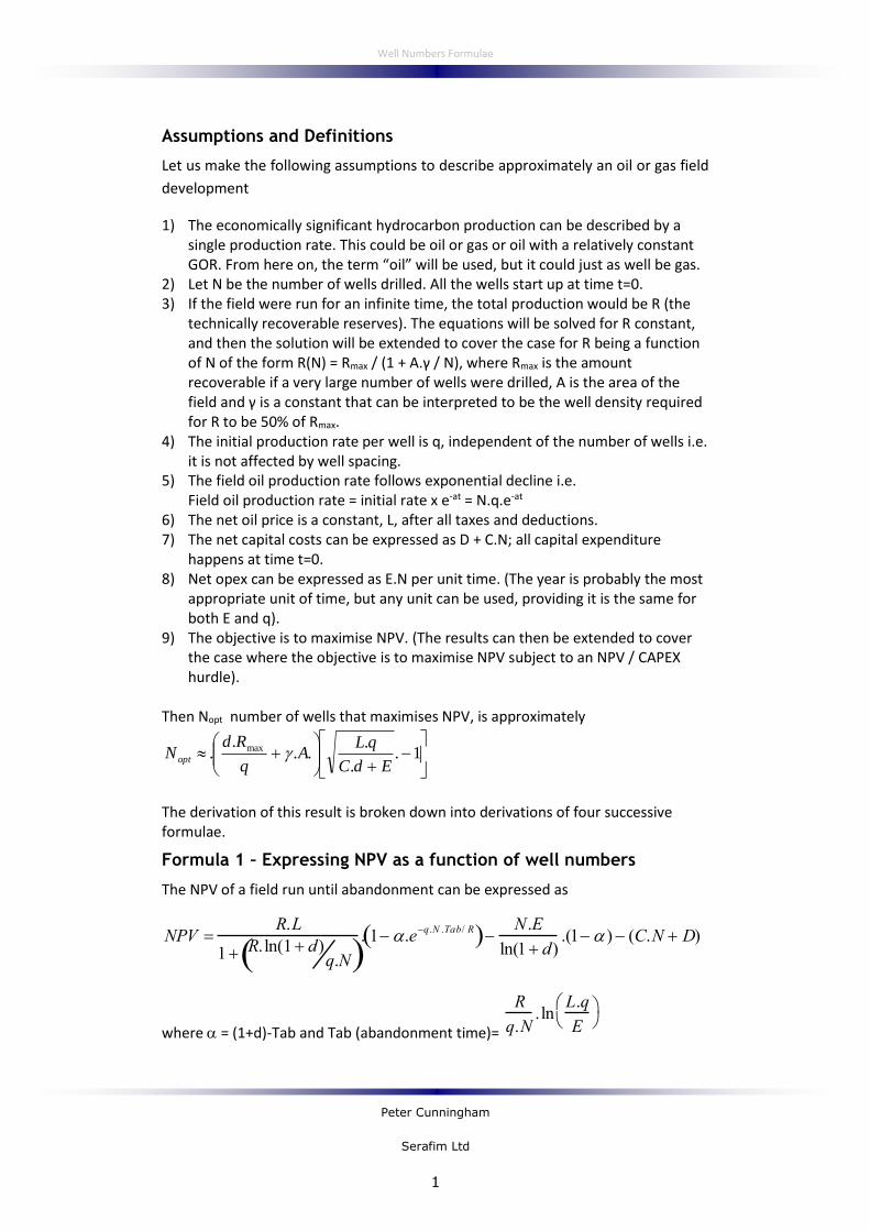
Assumptions and Definitions

Let us make the following assumptions to describe approximately an oil or gas field

development

1) The economically significant hydrocarbon production can be described by a single production rate. This could be oil or gas or oil with a relatively constant GOR. From here on, the term “oil” will be used, but it could just as well be gas.

2) Let N be the number of wells drilled. All the wells start up at time t=0. 3) If the field were run for an infinite time, the total production would be R (the

technically recoverable reserves). The equations will be solved for R constant, and then the solution will be extended to cover the case for R being a function of N of the form R(N) = Rmax / (1 + A.γ / N), where Rmax is the amount recoverable if a very large number of wells were drilled, A is the area of the field and γ is a constant that can be interpreted to be the well density required for R to be 50% of Rmax.

4) The initial production rate per well is q, independent of the number of wells i.e. it is not affected by well spacing.

5) The field oil production rate follows exponential decline i.e. Field oil production rate = initial rate x e-at = N.q.e-at

6) The net oil price is a constant, L, after all taxes and deductions. 7) The net capital costs can be expressed as D + C.N; all capital expenditure

happens at time t=0. 8) Net opex can be expressed as E.N per unit time. (The year is probably the most

appropriate unit of time, but any unit can be used, providing it is the same for both E and q).

9) The objective is to maximise NPV. (The results can then be extended to cover the case where the objective is to maximise NPV subject to an NPV / CAPEX hurdle).

Then Nopt number of wells that maximises NPV, is approximately

1.

.

...

.. max

EdC

qLA

q

RdN opt

The derivation of this result is broken down into derivations of four successive formulae.

Formula 1 – Expressing NPV as a function of well numbers

The NPV of a field run until abandonment can be expressed as

NPV R.L

1 R. ln(1 d)q.N

. 1 .eq.N .Tab/ R

N .E

ln(1 d).(1 ) (C.N D)

where = (1+d)-Tab and Tab (abandonment time)=

R

q.N. ln

L.q

E

Well Numbers Formulae

Peter Cunningham

Serafim Ltd

2

and

q – initial oil production per well per year, averaged over all wells, including

injectors

N – total number of wells, including injectors

R – technical reserves i.e. the amount of oil that could be recovered if the field

were run for a very long time (taken, at this stage, to be constant)

L – net revenue per unit of oil (i.e. after all taxes and royalties, including profit tax)

d – discount rate

C – net capital cost per well

D – net capital costs not related to numbers of wells, e.g. roads and pipelines

E – net opex per well

PROOF

NPV can be broken down into the component parts of the cash-flow

NPV = NPV(revenue stream) + NPV(Opex) + NPV(Capex)

where the NPV(Opex) and NPV(Capex) are, of course, negative.

Start by calculating the NPV of the revenue stream:-

By the assumption that there is exponential decline

Oil production rate = N.q.e-at = N.q.e-(q.N/R)t

[Since, by the definition of technical reserves

R N.q.ea.tdt

0

N.q

a.e

at

0

N.q / a

then a = N.q/R ]

Oil revenue per unit time = (production rate) x (net oil price) = N.L.q.e-q.N.t/R

By the definition of NPV

Well Numbers Formulae

Peter Cunningham

Serafim Ltd

3

NPV of revenue stream Revenue per unit time

(1 d)tdt

0

Tab

N .L.q.e (q.N / R ln(1 d)). tdt0

Tab

(Since (1 d)t e

ln((1d ) t ) e

t .ln(1d ))

N.L.q.e(q.N /R ln(1 d)) t

(q.N

R ln(1 d))

0

Tab

N.L.q

q.N

R ln(1 d)

. 1 e(q.N / Rln(1d )).Tab

R.L

1R. ln(1 d)

q.N

. 1 e ln(1 d). Tab

.e q.N.Tab/ R

R.L

1R. ln(1 d)

q.N

. 1 (1 d)Tab

.e q.N.Tab/ R

R.L

1R. ln(1 d)

q.N

. 1 .e q.N .Tab / R

Looking at the Opex cash-flow

Opex per unit time = -N.E

NPV of opex N.E

(1 d)tdt

0

Tab

N.E.e ln(1 d). tdt0

Tab

N.E.e ln(1 d).t

ln(1 d)0

Tab

N.E

ln(1 d). 1 e ln(1 d). Tab

N.E

ln(1 d). 1 (1 d)Tab

N.E

ln(1 d). 1

Looking at Capex, since all the capital expenditure is assumed to occur at time t=0,

NPV of Capex = - (C.N + D)

By adding NPV(Revenue), NPV(Opex) and NPV(Capex), one obtains the desired

formula.

Q.E.D

Formula 2 – Number of wells giving the highest NPV

Part I – The number of wells giving the highest NPV, Nopt, can be calculated

(iteratively) from the expressions

Well Numbers Formulae

Peter Cunningham

Serafim Ltd

4

Nopt R

q. ln(1 d).

L.q .E

C. ln(1 d) E .Ex 2 1 1

where .E. ln

L.q

E

4 L.q .E . C. ln(1 d) E .E

and (1 d)Tab

and Tab R

q.N. ln

L.q

E

Part II – If

L.q 2.[C.ln(1+d) + E] (i.e. the well is reasonably profitable at first) and

0.2 (equates, for d = 8%, to a field life 20 years)

then the approximation of setting = 0 gives approximate value for the number of

wells, Napprox within the following bounds

1.31 Nopt Napprox Nopt

Proof of Part I

Consider NPV as a function of well numbers and abandonment time. For a normally

behaved function

e.expenditur operating equalsit until dropped has revenue when occurs that thisseeingby

simply, more or, sderivative partial theby taking done becan 0Tab

NPVsuch that Tab Finding

0Tab

NPV

N

NPV maximum a is NPV

i.e. N.L.q.e-q.N.Tab/R = N.E

so –q.N.Tab/R = ln(E/(L.q))

so Tab = R/(q.N) . ln(L.q/E)

Well Numbers Formulae

Peter Cunningham

Serafim Ltd

5

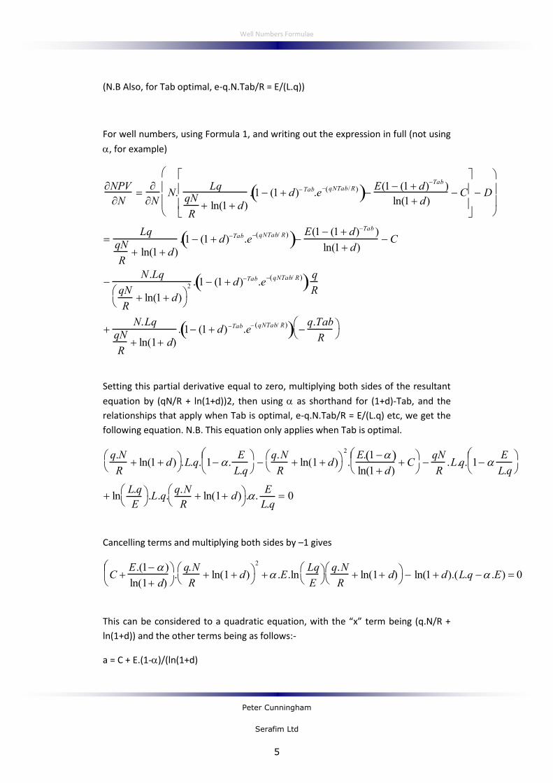
(N.B Also, for Tab optimal, e-q.N.Tab/R = E/(L.q))

For well numbers, using Formula 1, and writing out the expression in full (not using

, for example)

NPV

N

NN.

LqqN

R ln(1 d)

. 1 (1 d)Tab.e qNTab/R E(1 (1 d)

Tab)

ln(1 d)C

D

Lq

qN

R ln(1 d)

. 1 (1 d)Tab.e qNTab/ R

E(1 (1 d)Tab )

ln(1 d)C

N .Lq

qN

R ln(1 d)

2 . 1 (1 d)Tab.e qNTab/ R .

q

R

N.Lq

qN

R ln(1 d)

. 1 (1 d)Tab.e qNTab/ R .

q.Tab

R

Setting this partial derivative equal to zero, multiplying both sides of the resultant

equation by (qN/R + ln(1+d))2, then using as shorthand for (1+d)-Tab, and the

relationships that apply when Tab is optimal, e-q.N.Tab/R = E/(L.q) etc, we get the

following equation. N.B. This equation only applies when Tab is optimal.

q.N

R ln(1 d)

.L.q. 1 .

E

L.q

q.N

R ln(1 d)

2

.E. 1

ln(1 d)C

qN

R.L.q. 1

E

L.q

lnL.q

E

.L.q.

q.N

R ln(1 d)

..

E

L.q 0

Cancelling terms and multiplying both sides by –1 gives

C E.(1 )

ln(1 d)

.q.N

R ln(1 d)

2

.E.lnLq

E

q.N

R ln(1 d)

ln(1 d).(L.q .E) 0

This can be considered to a quadratic equation, with the “x” term being (q.N/R +

ln(1+d)) and the other terms being as follows:-

a = C + E.(1-)/(ln(1+d)

Well Numbers Formulae

Peter Cunningham

Serafim Ltd

6

b = .E.ln(L.q/E)

c = -ln(1+d).(L.q - .E)

We will proceed here in Part I of this proof to solve the quadratic equation. In Part

II, we will show that the “b” term has little effect, and can be ignored. (It is

interesting to consider how the “b” term arose. Consider the NPV of the field. If the

number of wells increases, then abandonment is brought forward, so the term

representing the present value of the oil lost at abandonment is increased. This

decreases the overall NPV, but as can be imagined, such effects are small. This will

be proved later, in Part II).

So, ignoring the negative solution, the solution of the quadratic equation is:

x b2 4a.c b

2a

Re - arranging this gives

x c

a. 1

b

4a.c

2

b

4a.c

Defining by b

4a.c

.E. lnL.q

E

4. C. ln(1 d) E .E . L.q .E

and expanding x, c and a gives

q.N

R ln(1 d)

ln(1 d).(L.q .E)

C E.(1 )

ln(1 d)

. 21

ln(1 d)(L.q .E)

C. ln(1 d) E .E. 2 1

Re - arranging this equation gives

N R

q. ln(1 d).

(L.q .E)

C. ln(1 d) E .E. 2 1 1

Proof of Formula 2, Part II

As a first step, it is useful to note that, for 0 (which is the case, providing L.q E

– i.e. Year 1 net revenue for a well is greater than the opex for the well)

Well Numbers Formulae

Peter Cunningham

Serafim Ltd

7

1 ((2+1) - ) 1- hence, Napprox Nopt

[ Proof - 21

2

21 2

2 1

2 1 2.

21 1

since 21 ]

Examining 2 and dividing both the denominator and quotient by (L.q)2 gives

2 ln L.q E

2 2 E L.q

2

4C. ln(1 d) (1 ).E

L.q

1

E

L.q

Since E

L.qC. ln(1 d) E

L.q 0.5 (by assumption 1) and 0.2 (by assumption 2)

1E

L.q

1 0.2x0.5 0.9

Also

C. ln(1 d) (1 ).E

L.q (1 ).

E

L.q 0.8

E

L.q

Hence,

2

ln L.q E 20.22 E L.q

2

4x0.8x E L.q x0.9 0.014 ln L.q E

2.E

L.q

It can be easily shown that for 1 E/(L.q) 0, the maximum value of

(ln(L.q/E))2.E/(L.q) is achieved when E/(L.q) = 1/(e2) = 0.1353, which gives

(ln(L.q/E))2.E/(L.q) = 0.541.

[Proof - Differentiate x.(ln(x))2 and set to zero].

Hence 0.014 x 0.541 = 0.00757

0.087

((1+2) - ) (1- ) (1-0.087) = 0.93

Before moving on to look at a lower limit for Nopt/Napprox, it is useful to establish

a couple of small lemmas.

Lemma A

Well Numbers Formulae

Peter Cunningham

Serafim Ltd

8

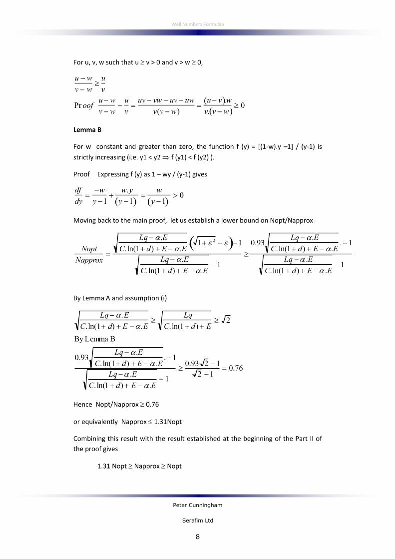
For u, v, w such that u v > 0 and v > w 0,

u w

v wu

v

Pr oof uw

v wu

vuv vw uv uw

v(v w)u v .w

v. v w 0

Lemma B

For w constant and greater than zero, the function f (y) = [(1-w).y –1] / (y-1) is

strictly increasing (i.e. y1 < y2 f (y1) < f (y2) ).

Proof Expressing f (y) as 1 – wy / (y-1) gives

df

dy

w

y 1w.y

y 1

w

y 1 0

Moving back to the main proof, let us establish a lower bound on Nopt/Napprox

Nopt

Napprox

Lq .E

C. ln(1 d) E .E. 1 2 1

Lq .E

C. ln(1 d) E .E1

0.93Lq .E

C. ln(1 d) E .E.1

Lq .E

C. ln(1 d) E .E1

By Lemma A and assumption (i)

Lq .E

C. ln(1 d) E .E

Lq

C. ln(1 d) E 2

By Lemma B

0.93Lq .E

C. ln(1 d) E .E.1

Lq .E

C. ln(1 d) E .E 1

0.93 2 1

2 1 0.76

Hence Nopt/Napprox 0.76

or equivalently Napprox 1.31Nopt

Combining this result with the result established at the beginning of the Part II of

the proof gives

1.31 Nopt Napprox Nopt

Well Numbers Formulae

Peter Cunningham

Serafim Ltd

9

Q.E.D.

Note – the formula for the approximately optimal number of wells can be further

simplified by noting that, for small d, ln(1+d) ≈ d

So if we ignore both the ε and α terms

1..

...

.

11..)1ln(.

)..().1ln(.N 2

EdC

qL

q

dRN

EEdC

EqLd

q

R

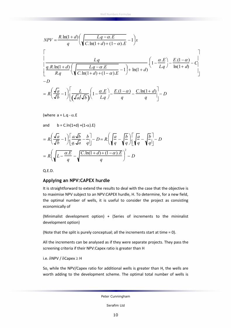
Formula 3 – NPV for a development with the approximately optimal number of wells

The NPV of a development with the approximately optimal number of wells, as

defined in Formula 2, is

NPV R. L .E

qC.ln(1 d) (1 ).E

q

2

D

where = (1+d)-Tab

and Tab = R / (N.q) . ln(L.q/E)

Proof

Combining the results from Formulas 1 and 2

Well Numbers Formulae

Peter Cunningham

Serafim Ltd

10

NPV R. ln(1 d)

q

L.q .E

C. ln(1 d) (1 ).E1

x

L.q

q.R. ln(1 d)

R.q.

L.q .E

C. ln(1 d) (1 ).E1

ln(1 d)

. 1 .E

L.q

E.(1 )

ln(1 d)C

D

R.a

b1

.

L

a b . 1

.E

L.q

E.(1 )

qC. ln(1 d)

q

D

(where a = L.q - .E

and b = C.ln(1+d) +(1-).E)

R.a

b1

.a. b

q. ab

q

D R.

a

qb

q

.

a

q

b

q

D

R. L .E

qC. ln(1 d) (1 ).E

q

2

D

Q.E.D.

Applying an NPV:CAPEX hurdle

It is straightforward to extend the results to deal with the case that the objective is

to maximise NPV subject to an NPV:CAPEX hurdle, H. To determine, for a new field,

the optimal number of wells, it is useful to consider the project as consisting

economically of

(Minimalist development option) + (Series of increments to the mininalist

development option)

(Note that the split is purely conceptual; all the increments start at time = 0).

All the increments can be analysed as if they were separate projects. They pass the

screening criteria if their NPV:Capex ratio is greater than H

i.e. NPV / Capex H

So, while the NPV/Capex ratio for additional wells is greater than H, the wells are

worth adding to the development scheme. The optimal total number of wells is

Well Numbers Formulae

Peter Cunningham

Serafim Ltd

11

reached when the limit is reached, so the criteria for determining the total number

of wells is

NPV / Capex = H

This can be converted into a more workable criterion as follows

NPV / Capex = H

(NPV-H.Capex) / Capex = 0

[(NPV-H.Capex) / N] x [N / Capex] = 0 where N is the number of wells

(NPV-H.Capex) / N = 0 since N / Capex 0 (it never costs an

infinite amount of money to drill a new well).

Hence, the new problem (find the number of wells that maximises corporate NPV

subject to a limit on capital employed) can be converted into the old (find the

number of wells that maximises NPV) by using an artifical NPV, defined to be

NPV = NPV – H.Capex = NPV – H.(C.N + D)

and artificial C and D defined to be

C = (1 + H) x C

D = (1 + H) x D

Formula 4 - When ultimate recovery depends on well numbers

The results so far have been derived under the assumption that technical ultimate

recovery R is independent of the number of wells drilled, N. The results can be

extended to cover the case where R is a function of N of the form R(N) = Rmax / (1

+ A.γ / N), where Rmax is the amount recoverable if a very large number of wells

were drilled, A is the area of the field and γ is a constant that can be interpreted to

be the well density required for R to be 50% of Rmax. This extension gives rise to

some interesting measures of the economics of a field / technology combination –

the “production” and “recovery” costs:revenue ratios.

In many fields, particularly medium permeability gas fields with limited aquifers, it

is reasonable to approximate field ultimate recovery as being independent of well

numbers. However, there are many other fields, such heavy oil fields or low

permeability gas fields in which the number of wells drilled has a big effect on field

ultimate recovery.

A first point to note is that reservoir simulation generally suggests that increases in

well numbers lead to increases in field ultimate recovery. There was an old

Well Numbers Formulae

Peter Cunningham

Serafim Ltd

12

argument, based on the Buckley-Leverett model (a 2D analytical model of

immiscible displacement) applied to segregated flow that suggested that high well

numbers could, in those circumstances, lead to unstable flow – “viscous fingering”

– and lower ultimate recoveries. However, simulation models, which give a more

complete 3D picture of fluid flow, suggest that, in practice, such a reduction in field

ultimate recovery does not easily occur.

Instead, it can be argued that field recovery factor will increase with increasing

number and will approach asymptotically the microscopic recovery factor for the

relevant drive mechanism. It is not known for certain what form the R vs N

relationship should take. In some ways, it is possibly not so important which family

of curves is chosen, providing the curves go through whatever calibration points

are available and honour the asymptote. However, good results have been

obtained in heavy oil fields, such as the Alba field in the North Sea, using, as

described in SPE 71833, a relationship of the form

R(N) = Rmax / (1 + A.γ / N) where

Rmax = the asymptotic value i.e. the amount recoverable if a very large number of

wells were drilled, which can be estimated to be STOIIP (or GIIP) x microscopic

recovery factor;

A = the area of the field;

γ = a constant that can be adjusted to fit the calibration points (e.g. simulation

runs; extrapolations in time of production history to date); it can be interpreted

(from the formula) to be the well density required for R to be 50% of Rmax.

(Note – this equation is, in fact, a special case, for b = ½ , of the more general

procedure of fitting an Arps hyperbolic equation to dUR(N)/dN vs UR(N) in place of

the conventional dQ(t)/dt vs Q(t) ).

The plot below illustrates how, for part of the Alba field (AXS = “Alba Extreme

South”), such a curve fitted to a single simulation run (in red) and to the calculated

Rmax succeeded in predicting closely the ultimate recovery from three other

simulation runs. NB – the plot is shown in terms of producing horizontal well

footage, but the concepts are the same as for well numbers.

Well Numbers Formulae

Peter Cunningham

Serafim Ltd

13

When it comes to incorporating R(N) into field development optimisation, we will

confine ourselves to the simple case where we

ignore abandonment effects (so time runs to infinity)

the discount rate, d, is in the normal range, so ln(1+d) can be approximated by d.

In these circumstances, for our development with N wells, the decline exponent

and consequently the NPV are given by the equations

DNd

ECdteqNL

DNd

ECdteqNL

DNd

ECdt

e

eqNLDN

d

ECdt

d

eqNLNPV

R

N

AqN

R

qNa

tdR

qA

R

qN

tdR

qA

R

qN

dt

tR

qA

R

qN

t

at

.....

.....

.....

.1

...

1...

0

..

0

)1ln(..

0

)1ln(.

..

0

max

maxmax

maxmax

maxmax

AXS area - Effects of well density on recovery

0

50

100

150

200

250

0 20 40 60 80 100 120

Well footage (1000 ft)

Ult

ima

te r

ec

ov

ery

in

20

20

(m

m

b)

0

2

4

6

8

10

12

14

16

18

Ad

dit

ion

al

rec

ov

ery

pe

r 1

00

0 f

t

(mm

b)

UR

Calibration to simulation

Validation to additionalsimulation runs

Additional rec per well

Well Numbers Formulae

Peter Cunningham

Serafim Ltd

14

since ln(1+d) ≈d for small d (<0.3)

This is an equation of the same form as when R is constant, with the following

substitutions -

Term in old form (R constant) Term in new form (R a function of N)

R Rmax

d d + γ.A.q/ Rmax

C C+E/d

E 0

Making these substitutions into the approximate formula for the optimal number

of wells

1.

.

...

.

EdC

qL

q

dRNopt

Becomes

1..

...

..1.

.

...

...

maxmaxmax

EdC

qLA

q

Rd

EdC

qL

q

RqA

dR

Nopt