Derivation of Formulations 1 and 1A of Farassat - NASA · • TECHNICAL TRANSLATION. English- ......

March 2007

NASA/TM-2007-214853

Derivation of Formulations 1 and 1A of Farassat F. Farassat Langley Research Center, Hampton, Virginia

https://ntrs.nasa.gov/search.jsp?R=20070010579 2018-07-30T02:36:32+00:00Z

The NASA STI Program Office . . . in Profile

Since its founding, NASA has been dedicated to the advancement of aeronautics and space science. The NASA Scientific and Technical Information (STI) Program Office plays a key part in helping NASA maintain this important role.

The NASA STI Program Office is operated by Langley Research Center, the lead center for NASA’s scientific and technical information. The NASA STI Program Office provides access to the NASA STI Database, the largest collection of aeronautical and space science STI in the world. The Program Office is also NASA’s institutional mechanism for disseminating the results of its research and development activities. These results are published by NASA in the NASA STI Report Series, which includes the following report types:

• TECHNICAL PUBLICATION. Reports of

completed research or a major significant phase of research that present the results of NASA programs and include extensive data or theoretical analysis. Includes compilations of significant scientific and technical data and information deemed to be of continuing reference value. NASA counterpart of peer-reviewed formal professional papers, but having less stringent limitations on manuscript length and extent of graphic presentations.

• TECHNICAL MEMORANDUM. Scientific

and technical findings that are preliminary or of specialized interest, e.g., quick release reports, working papers, and bibliographies that contain minimal annotation. Does not contain extensive analysis.

• CONTRACTOR REPORT. Scientific and

technical findings by NASA-sponsored contractors and grantees.

• CONFERENCE PUBLICATION. Collected

papers from scientific and technical conferences, symposia, seminars, or other meetings sponsored or co-sponsored by NASA.

• SPECIAL PUBLICATION. Scientific,

technical, or historical information from NASA programs, projects, and missions, often concerned with subjects having substantial public interest.

• TECHNICAL TRANSLATION. English-

language translations of foreign scientific and technical material pertinent to NASA’s mission.

Specialized services that complement the STI Program Office’s diverse offerings include creating custom thesauri, building customized databases, organizing and publishing research results ... even providing videos. For more information about the NASA STI Program Office, see the following: • Access the NASA STI Program Home Page at

http://www.sti.nasa.gov • E-mail your question via the Internet to

[email protected] • Fax your question to the NASA STI Help Desk

at (301) 621-0134 • Phone the NASA STI Help Desk at

(301) 621-0390 • Write to:

NASA STI Help Desk NASA Center for AeroSpace Information 7115 Standard Drive Hanover, MD 21076-1320

National Aeronautics and Space Administration Langley Research Center Hampton, Virginia 23681-2199

March 2007

NASA/TM-2007-214853

Derivation of Formulations 1 and 1A of Farassat F. Farassat Langley Research Center, Hampton, Virginia

Available from: NASA Center for AeroSpace Information (CASI) National Technical Information Service (NTIS) 7115 Standard Drive 5285 Port Royal Road Hanover, MD 21076-1320 Springfield, VA 22161-2171 (301) 621-0390 (703) 605-6000

This publication is based on a lecture delivered by the author to the staff of the Aeroacoustics Branch of NASA Langley Research Center on Monday, October 23, 2006. Acknowledgments The author thanks Mr. Seongkyu Lee and Mr. Leonard Lopes of Penn State, Dr. Damiano Casalino of CIRA, Italy and Mr. Ghader Ghorbaniasl of University of Brussels, Belgium for their valuable comments which improved the clarity of the presentation of this publication. The author is grateful for the useful comments he received from Drs. Douglas M. Nark and D. Douglas Boyd who were the official reviewers of this publication. Dr. Jay Casper and Ms. Martha Brown supplied figures 1 and 2, respectively.

Derivation of Formulations 1 and 1A of Farassat

F. FarassatNASA Langley Research Center, Hampton, Virginia

SummaryFormulations 1 and 1A are the solutions of the Ffowcs Williams-Hawkings (FW-H) equation withsurface sources only when the surface moves at subsonic speed. Both formulations have been success-fully used for helicopter rotor and propeller noise prediction for many years although we now recom-mend using Formulation 1A for this purpose. Formulation 1 has an observer time derivative that is takennumerically, and thus, increasing execution time on a computer and reducing the accuracy of the results.After some discussion of the Green’s function of the wave equation, we derive Formulation 1 which isthe basis of deriving Formulation 1A. We will then show how to take this observer time derivativeanalytically to get Formulation 1A. We give here the most detailed derivation of these formulations.Once you see the whole derivation, you will ask yourself why you did not do it yourself!

1- Primary ReferencesFormulation 1 was first published in:

1- F. Farassat: Theory of Noise Generation From Moving Bodies With an Application to Helicop-ter Rotors, NASA Technical Report R-451, 1975However, the derivation of this formulation in this reference is very difficult. Later, I found a muchsimpler derivation which we will follow here. It was published in:

2- F. Farassat: Linear acoustic formulas for calculation of rotating blade noise, AIAA Journal,19(9), 1981, 1122-1130 Formulation 1A was first published in:

3- F. Farassat, G. P. Succi, A review of propeller discrete frequency noise prediction technologywith emphasis on two current methods for time domain calculations, 1980, Journal of Sound andVibration, 71(3), 399-419

In deriving the formulation in the above reference, I assumed, as it was common then, that the bladesurface did not move out of the disc plane. This assumption was removed by Kenneth S. Brentner andwas published in the following excellent NASA Technical Memorandum:

4- Kenneth S. Brentner, Prediction of Helicopter Discrete Frequency Rotor Noise- A ComputerProgram Incorporating Realistic Blade Motions and Advanced Formulation, October 1986,NASA TM 87721We refer to the result published in this paper as Formulation 1A. At the time of writing Reference 3,we at Langley had not started numbering and identifying our formulations. In hindsight, it was a goodidea to identify each of our formulations because different codes use different results. Our numberingsystem has worked for identifying what formulation is used in a code. Formulation 1A has been used inhelicopter rotor noise prediction codes WOPWOP and PSU-WOPWOP, and together with our super-sonic Formulation 3, in our advanced propeller noise prediction code ASSPIN (Advanced Subsonicand Supersonic Propeller Induced Noise).

You will need much mathematical maturity to follow what we discuss here. To understand the mathemat-ics behind our work, I strongly recommend reading Reference 1, above, and the following two NASApublications:

5- F. Farassat, Introduction to Generalized Functions With Applications in Aerodynamics andAeroacoustics, May 1994 (Corrected April 1996), NASA Technical Paper 34286- F. Farassat: The Kirchhoff Formulas for Moving Surfaces in Aeroacoustics - The Subsonic andSupersonic Cases, NASA Technical Memorandum 110285, September 1996Reference 6 was written to clarify and fill in some gaps in the mathematical analysis of Reference 5. Itshould be read together with the latter reference.

2- The Ffowcs Williams-Hawkings (FW-H) EquationThis equation was first published in:

7- J. E. Ffowcs Williams and D. L. Hawkings: Sound generated by turbulence and surfaces inarbitrary motion, Philosophical Transactions of the Royal Society, A264, 1969, 321-342 This paper is very difficult to read because of the high level of mathematics needed to follow theauthors’ reasoning. There are many original ideas in this paper such as the idea of imbedding a problemin a larger domain to use the available Green’s function of the larger domain to solve the original prob-lem. Another idea put forward by Ffowcs Williams and Hawkings is that conservation laws in differen-tial form are also valid when all ordinary derivatives are viewed as generalized derivatives. This hasimportant implications about the jump conditions across flow discontinuities. I have given the back-ground mathematics needed to understand this paper in References 1, 5 and 6.

Ffowcs Williams-Hawkings (FW-H) Equation as originally proposed in Reference 7 above:

2 Farassat Formulations 1 and 1A.nb

(1)·2 p ' =

ÅÅÅÅÅÅÅÅ t

@r0 vn dH f LD -

ÅÅÅÅÅÅÅÅÅÅÅ xi

@p ni dH f LD +2

ÅÅÅÅÅÅÅÅÅÅÅÅÅÅÅÅÅÅÅÅÅÅ xi xj

@HH f L TijD

Here and elsewhere in the paper, we will use the summation convention on the repeated index. In thisequation ·2 is the wave or D’Alembertian operator in three dimensional space. The moving surface isdescribed by f Hx, tL = 0 such that ıf = n , n is the unit outward normal. This assumption implies thatf > 0 outside the moving surface (see Figure 1). Also p ' = c2 r ' = c2Hr - r0L , c and r0 are the speedof sound and density in the undisturbed medium, respectively. Note that p£ can only be interpreted asthe acoustic pressure if r£ ê r0 << 1. The symbols vn , p and Tij = r ui uj - sij + Ip£ - c2 r 'M dij are thelocal normal velocity of the surface, the local gage pressure on the surface (in fact p - p0 ), and theLighthill stress tensor, respectively. In the definition of the Lighthill stress tensor, sij is the viscousstress tensor and dij is the Kronecker delta. The Heaviside and the Dirac delta functions are denotedHH f L and dH f L , respectively. In the second term on the right of eq. (1), we have neglected the viscousshear force over the blade surface acting on the fluid.

Figure 1- The definition of the moving surface implicitly as f Hx, tL = 0 . Note that ı f = n where nis the unit outward normal to the surface.We note that we have artificially converted a nonlinear problem of noise generation by a moving surfaceto a linear problem by using the acoustic analogy. All the nonlinearities are lumped into the Lighthillstress tensor which is assumed known from near field aerodynamic calculations. When we started work-ing on helicopter and propeller noise in the early seventies, because of the limitations of digital comput-ers, the most we could expect from aerodynamic calculations was the blade surface pressure. For thisreason, using some physical reasoning, we neglected the quadrupole volume sources in FW-H equationand concentrated on development of formulations for the prediction of thickness and loading noise.Later on, as computers became more powerful, we included quadrupoles in our noise prediction. Therewas, however, another theoretical advance which led to the use of purely surface sources to which wewill turn next.

It was Ffowcs Williams himself who proposed to use a penetrable (porous or permeable) data surface toaccount for nonlinearities in the vicinity of a moving surface. We again assume that the penetrablesurface defined by f Hx, tL = 0 and the fluid velocity is denoted by u . The FW-H equation for penetra-ble (permeable, porous) data surface, FW-Hpds , is:

Farassat Formulations 1 and 1A.nb 3

(2)Ñ 2 c2 r£ ª Ñ 2 p£ =

ÅÅÅÅÅÅÅÅ t

@r0 UnD dH f L -


@Li dH f LD +2

ÅÅÅÅÅÅÅÅÅÅÅÅÅÅÅÅÅÅÅÅÅÅ xi xj

@Tij HH f LD

We have used the following notations in the above equation:

(3)Un = ikjj1 -

rÅÅÅÅÅÅÅÅÅr0

y{zz vn +

r unÅÅÅÅÅÅÅÅÅÅÅÅÅr0

(4)Li = p d ij nj + r ui Hun - vnLwhere dij is the Kronecker delta. As in the case of eq. (1), in the first term on the right of eq. (4), wehave neglected the viscous shear force over the data surface acting on the fluid exterior to the surface.The philosophy behind using FW-Hpds is to locate the data surface f = 0 to enclose a moving surface,in such a way that all quadrupoles producing non-negligible noise are included within this surface.Therefore, no volume integration of the quadrupoles outside the data surface is necessary. High resolu-tion CFD calculation is performed in the near field region (including turbulence simulation if broadbandnoise prediction is required). The data surface used for the acoustic calculation should be located withinthe region of high resolution CFD computation. The optimal location of the data surface, particularlywhen vortices cross the surface, is still the subject of research. One would like this surface to be as smallas possible, because of the computer intensive nature of aerodynamic and turbulence simulation thatrequire fine grid sizes and small time steps.

We will be concerned with the solution of the following two wave equations:

(5)Ñ 2 p£T =

ÅÅÅÅÅÅÅÅ t

@r0 vn dH f LD Thickness Noise Equation

(6)Ñ 2 p£L = -


@p ni dH f LD Loading Noise Equation

The source terms on the right of eqs. (5) and (6) are known also as monopole and dipole sources, respec-tively. This terminology is misleading for sources on a moving surface because the radiation patternscalculated from the above equations are not similar to those from stationary monopoles and dipoles. Infact, we can show mathematically that the thickness noise is equivalent to the loading noise from auniform surface pressure distribution of magnitude r0 c2 . For this reason we avoid using the terminol-ogy of monopole and dipole sources here.

Remark 1- We will now give an example of a moving surface defined implicitly by f = 0. A sphere ofradius a moving at the speed v along the x1-axis is described by the equation:

(7)f1 = Hx1 - v tL2 + x22 + x3

2 - a2 = 0

Note that f1 > 0 outside the surface, and f1 < 0 inside it. Now let us test the gradient of this function.We see that

(8)ı f1 = H2 Hx1 - v tL, 2 x2, 2 x3L n = J x1 - v tÅÅÅÅÅÅÅÅÅÅÅÅÅÅÅÅÅÅÅÅÅ

a,

x2ÅÅÅÅÅÅÅÅa

,x3ÅÅÅÅÅÅÅÅaN


We have †ı f1 § = 2 "######################################Hx1 - v tL2 + x22 + x3

2 . Therefore, we redefine the moving sphere by the equation:

(9)f Hx, tL =f1ÅÅÅÅÅÅÅÅÅÅÅÅÅÅÅÅ†ı f1 § =

1ÅÅÅÅÅ2

"#####################################Hx1 - v tL2 + x22 + x3

2 -a2

ÅÅÅÅÅÅÅÅÅÅÅÅÅÅÅÅÅÅÅÅÅÅÅÅÅÅÅÅÅÅÅÅÅÅÅÅÅÅÅÅÅÅÅÅÅÅÅÅÅÅÅÅÅÅÅÅÅÅÅÅÅÅÅÅÅÅÅ2 "#####################################Hx1 - v tL2 + x2

2 + x32

= 0

We give the following general rule: if ı f n on the surface f = 0, then redefine the same surface bythe implicit equation f ê †ı f § = 0. We can then show that ı H f ê †ı f §L = n on this surface. The proof issimple.

Note that a surface can be defined implicitly in more than one way satisfying the condition ı f = n . Forexample, for the above surface a much simpler representation in implicit form satisfying this conditionis f Hx, tL = "######################################Hx1 - v tL2 + x2

2 + x32 - a = 0.

We have not said anything about why we require the condition †ı f § = 1 on the surface. The FW-Hequation as it was originally written in Reference 7 had the term †ı f § in both the thickness and loadingterms. We have been assuming †ı f § = 1 in writing the FW-H equation in all of our publications formany years. To begin with, we notice that the term †ı f § does not appear in both Formulations 1 and 1A.In the process of the derivation of some of our more advanced formulations where the source time andspace derivatives of †ı f § were required, I noticed that all terms associated with these derivatives can-celed out exactly in the final result. After considerable search for the reason or reasons behind thiscancellation, I discovered that †ı f § = 1 could be assumed to be true on any surface described implicitlyfrom the beginning of the derivation of FW-H equation. This explained the reason for cancellation of theterms associated with the derivatives of †ı f § in our advanced formulations. Although this assumption isof little value in the derivation of Formulation 1, it reduces the algebra somewhat in the derivation ofFormulation 1A and enormously in our advanced formulations. (End of Remark 1)

3- Background Material and the Details of the Derivation3.1- Green’s Function of the Wave Equation in Unbounded Three Dimensional SpaceThe Green’s function of the wave equation in the unbounded three dimensional space is:

(10)GHx, t; y, tL = ; 0 t > td Ht - t + r ê cL ê4 p r t b t

where r = † x - y § . Here Hx, tL and Hy, tL are the observer and the source space-time variables, respec-tively. In the above equation, the symbol dH ÿ L stands for the Dirac delta function which is the most well-known generalized function. We usually use the following symbol: g = t - t + r ê c . We will discuss inRemark 3 below how we visualize and interpret the function g = 0. See also References 1 and 5 above.

The Green’s function given by eq. (10) is also known as the free-space Green’s function.


Remark 2- It is a good idea to remember the following two simple results because they are frequentlyencountered in algebraic manipulations:

(11) r

ÅÅÅÅÅÅÅÅÅÅÅÅ x i

= r̀i and r

ÅÅÅÅÅÅÅÅÅÅÅÅ y i

= - r̀i

where r̀i is the component of the unit radiation vector Hx - yL ê r . (End of Remark 2)

Remark 3- The surface g = t - t + r ê c = 0 can be visualized as follows. Keep the observer space-timevariables fixed. Then let us first rewrite the equation of this surface as † x - y § = c Ht - tL . In the sourcespace-time variables, this surface is simply a sphere with center at x and radius equal to c Ht - tL . Notethat the Green’s function of the wave equation is nonzero when t b t , so that as the source timeincreases from t = -¶ to t = t , the radius of this sphere shrinks from infinitely large value to zero. Forthis reason this sphere is known as the collapsing sphere. The rate of contraction of the radius of thissphere is the speed of sound c .

Mathematically, the collapsing sphere is the characteristic cone of the wave equation with the vertex atHx, tL and the cone pointing towards the past. Causality rules out using the part of the cone pointingtowards the future. Can you think of a reason why this surface is called a cone? See Reference 6, abovefor the answer. (End of Remark 3)

3.2- Solution of the Wave Equation With Sources on a Mov-ing Surface We are interested in the solution of the equation:

(12)Ñ 2 p£ = QHx, tL dH f LWe will derive the solution of this equation using the free-space Green’s function given by eq. (10).This will show the interconnection between the variables that confuses novices in the field of aeroacous-tics. The formal solution of eq. (12) is:

(13)4 p p£ Hx, tL = ‡ QHy, tL dH f L dHgLÅÅÅÅÅÅÅÅÅÅÅÅÅ

r d y d t

The limits of the integral in this equation are given below:

(14)‡ ... .. d y d t = ‡-¶

t

‡!3

... .. d y d t = ‡-¶

t

‡-¶

¶

‡-¶

¶

‡-¶

¶

... .. d y1 d y2 d y3 d t

We emphasize at this point that the x - frame and the y - frame are fixed to the undisturbed medium.For the next analytic step, such a frame is not the most appropriate frame to interpret the solution of eq.(12) as we will show below. It is important to remember that from now on, the observer space-timevariables Hx, tL are kept fixed in all algebraic manipulations. Therefore, for all practical purposes, we aredealing with four variables Hy, tL . For problems of interest in aeroacoustics, such as propeller and helicopter rotor noise prediction, onecan always describe the surface (generally a blade) in a frame fixed relative to the surface. We will callthis frame the h - frame. Such a frame is used by the manufacturer to describe the design of the bladesurface to the technicians who build the blade. We call the variable h the Lagrangian variable of apoint on the moving surface. If we mark a point on the surface, say by a red dot, then we have essen-tially identified a point with the fixed variable h on the moving surface. In general, in the h-frame themoving surface is time independent although this does not have to be so in the following mathematicalmanipulations. The thing to realize at this point is that once the motion of the blade is specified, then thetrajectory of a point on the surface described by a fixed h is specified in space-time in the y-frame, i.e.,in space. This trajectory is given by the relation:


For problems of interest in aeroacoustics, such as propeller and helicopter rotor noise prediction, onecan always describe the surface (generally a blade) in a frame fixed relative to the surface. We will callthis frame the h - frame. Such a frame is used by the manufacturer to describe the design of the bladesurface to the technicians who build the blade. We call the variable h the Lagrangian variable of apoint on the moving surface. If we mark a point on the surface, say by a red dot, then we have essen-tially identified a point with the fixed variable h on the moving surface. In general, in the h-frame themoving surface is time independent although this does not have to be so in the following mathematicalmanipulations. The thing to realize at this point is that once the motion of the blade is specified, then thetrajectory of a point on the surface described by a fixed h is specified in space-time in the y-frame, i.e.,in space. This trajectory is given by the relation:

(15)y = y Hh, tLThe inverse transformation is given by:

(16)h = h Hy, tLNote that the equation of the moving surface f Hy, tL = 0 in the h-frame is f Hy Hh, tL, tL = f

è Hh, tL = 0. In

practice, fè

= 0 is independent of time, i.e., the surface is described as fè

HhL , and this is what we assumehere. Later on we will see that it is customary to use f when we should properly use f

è for designating

the moving surface in an analytic expression (e.g., see eq. (29)). This is an abuse of notation which isacceptable for the reason that we will discuss in the paragraph following eq. (31). You should keep inmind that, in general, the analytic expressions for f and f

è are different. For example, in the example of

a moving (rigid) sphere in Remark 1, we have f Hy, tL = "######################################Hy1 - v tL2 + y22 + y3

2 - a = 0 while

fè

HhL = "########################h12 + h2

2 + h32 - a = 0. Here, we are assuming that the h-frame has its origin at the center of the

sphere with its axes parallel to corresponding axes of the y-frame. However, this distinction does notmatter to us here because we are not able to integrate any of the acoustic integrals here in closed formfor any nontrivial moving surface. We always evaluate our surface integrals numerically by finite differ-ence scheme after we divide a data or a blade surface into panels.

For problems of interest to us in aeroacoustics, the transformations described by eqs. (15) and (16) areisometric, i.e., distance preserving, because they involve translations and rotations only. For this reason,the Jacobians of transformation are unity, that is, we have

(17)det ikjj y

ÅÅÅÅÅÅÅÅÅÅh

y{zz = 1 and det ik

jj hÅÅÅÅÅÅÅÅÅÅ y

y{zz = 1

If you have trouble accepting this, then use the translation transformation y = h + v t for a constantvelocity v used in Remark 1 (where v = v e1 and e1 is the basis vector along h1 - axis) to test the valid-ity of eq. (17). We now go back to the integration of the Dirac delta functions of eq. (13). We first usethe transformation y Ø h in this equation to get

(18)4 p p£ Hx, tL =

‡ QHyHh, tL, tL dH fèL dHgL

ÅÅÅÅÅÅÅÅÅÅÅÅÅÅÅÅÅÅÅÅÅÅÅÅÅÅÅÅÅÅÅÅÅÅÅÅÅÅÅÅÅÅr †det Hh ê yL§ dh d t = ‡

-¶

t ‡

!3Qè

Hh, tL dH fèL dHgL

ÅÅÅÅÅÅÅÅÅÅÅÅÅr

dh d t

where we have defined Qè

Hh, tL = QHyHh, tL, tL. Next we use the transformation t Ø g . The Jacobian ofthis transformation is g êt . Here the variable h is kept fixed in this partial differentiation. We will dothe algebra in detail below. First we have


(19)g = t - t +† x - y Hh, tL §ÅÅÅÅÅÅÅÅÅÅÅÅÅÅÅÅÅÅÅÅÅÅÅÅÅÅÅÅÅÅÅÅÅÅÅÅÅ

cThe partial differentiation with respect to variable t gives

(20)gÅÅÅÅÅÅÅÅÅt

= 1 +1ÅÅÅÅÅc

r

ÅÅÅÅÅÅÅÅÅÅÅyi

yiÅÅÅÅÅÅÅÅÅÅÅt

= 1 -r̀i viÅÅÅÅÅÅÅÅÅÅÅÅ

c= 1 - Mr

where M r = r̀ i vi êc is the Mach number of the point h in the radiation direction at the time t . Here r̀i isthe component of unit radiation vector Hx - yL ê r and vi = yi Hh, tL êt is the component of the velocityv of the point h with respect to the y - frame fixed to the undisturbed medium.

Using the above results in eq. (18) and assuming that is a small positive number, we get

(21)

4 p p£ Hx, tL = ‡ Qè

Hh, tL dH fèL dHgL

ÅÅÅÅÅÅÅÅÅÅÅÅÅÅÅÅÅÅÅÅÅÅÅÅÅÅÅÅr †g ê t§ dh d g =

‡!3‡

-

Qè

Hh, tL dH fèL dHgL

ÅÅÅÅÅÅÅÅÅÅÅÅÅÅÅÅÅÅÅÅÅÅÅÅÅÅÅr †1 - Mr § d g dh = ‡

!3

ikjjj Q

è Hh, tL

ÅÅÅÅÅÅÅÅÅÅÅÅÅÅÅÅÅÅÅÅÅÅÅÅÅÅÅr †1 - Mr § dH f

èLy{zzz

g=0 dh

Note that the limits of the inside integral (with respect to g) of the expression after the second equalitysign are from - to ( > 0) because dHgL could only contribute to the integral in this region. In whatfollows, we will drop the absolute value sign around †1 - Mr § because for surfaces moving subsonically,we always have 1 - Mr > 0. The expression 1 - Mr is known as the Doppler factor. Let us now inter-pret what exactly the condition g = 0 imposes on us. Remember that we have used the transformationt Ø g . This means that, from eq. (19), the condition g = 0 makes the source time dependent on the othervariables Hx, t; hL . This function is found analytically by solving for t from the equation

(22)g = t - t +† x - y Hh, tL §ÅÅÅÅÅÅÅÅÅÅÅÅÅÅÅÅÅÅÅÅÅÅÅÅÅÅÅÅÅÅÅÅÅÅÅÅÅ

c= 0 HHx, tL kept fixedL

Before we go further, let us see what this source time signifies. Remember that when we fix h , it meansthat we have marked a fixed point on the moving surface, say, with a red dot. Therefore, the trajectoryof this red dot in space-time is known from the relation y = y Hh, tL . That is, given any source time t ,we know where the red dot is on its trajectory in space. But from eq. (22), we have

(23)† x - y Hh, tL § = c Ht - tLLet us write te = t Hx, t; hL and ye = y Hh, teL . We will shortly say what the subscript e stands for. Withthese notations, eq. (23) can be written as

(24)re ª † x - ye § = c H t - teLClearly, the source time te is the emission time, ye = y Hh, teL is the emission position, and re is theemission distance of the source point h to the observer position x . Both the emission position and theemission distance are viewed in the y - frame fixed to the undisturbed medium. See Figure 2 for anillustration of some of the terms we use here. It can be shown that for a subsonically moving source,there is only one emission time for a given source point h . In practical problems of rotating blade noiseprediction, we cannot find a closed form analytic expression for t = te Hx, t; hL because eq. (23) is atranscendental equation involving sines and cosines. However, we can find te numerically easily by ashooting technique. Roughly speaking, here is what we do. At the observer time t , we know where thesource (the red dot) position is and its trajectory in space. This position is called the visual position ofthe source. Walk in small time steps along the trajectory back in (source) time, i.e., for t < t , and eachtime check to see if eq. (23) is satisfied. You may be overshooting the emission position y Hh, teL . Inthat case, walk along the trajectory towards the visual position of the source in smaller time steps tillyou find the emission time and position satisfying eq. (23). In practice, this method can be refinedconsiderably to speed up the computation of the emission time.


Clearly, the source time te is the emission time, ye = y Hh, teL is the emission position, and re is theemission distance of the source point h to the observer position x . Both the emission position and theemission distance are viewed in the y - frame fixed to the undisturbed medium. See Figure 2 for anillustration of some of the terms we use here. It can be shown that for a subsonically moving source,there is only one emission time for a given source point h . In practical problems of rotating blade noiseprediction, we cannot find a closed form analytic expression for t = te Hx, t; hL because eq. (23) is atranscendental equation involving sines and cosines. However, we can find te numerically easily by ashooting technique. Roughly speaking, here is what we do. At the observer time t , we know where thesource (the red dot) position is and its trajectory in space. This position is called the visual position ofthe source. Walk in small time steps along the trajectory back in (source) time, i.e., for t < t , and eachtime check to see if eq. (23) is satisfied. You may be overshooting the emission position y Hh, teL . Inthat case, walk along the trajectory towards the visual position of the source in smaller time steps tillyou find the emission time and position satisfying eq. (23). In practice, this method can be refinedconsiderably to speed up the computation of the emission time.

Figure 2- Sketch of the trajectory of a source point h (the red dot) as seen by an observer fixed tothe medium (x- or y-frame) and the definitions of visual and emission positions of the source

With the above notations, eq. (21) can be written as:

(25)4 p p£ Hx, tL = ‡!3

Qè

Hh, teLÅÅÅÅÅÅÅÅÅÅÅÅÅÅÅÅÅÅÅÅÅÅÅÅÅÅÅÅÅÅÅÅÅre H1 - Mre L dA f

è HhLE dh

where we have defined Mre = MHh, teL ÿ r̀e and MHh, teL = vHh, teL ê c . Now note that

(26)Qè

Hh, teLÅÅÅÅÅÅÅÅÅÅÅÅÅÅÅÅÅÅÅÅÅÅÅÅÅÅÅÅÅÅÅÅÅre H1 - Mre L = y Hx, t; hL


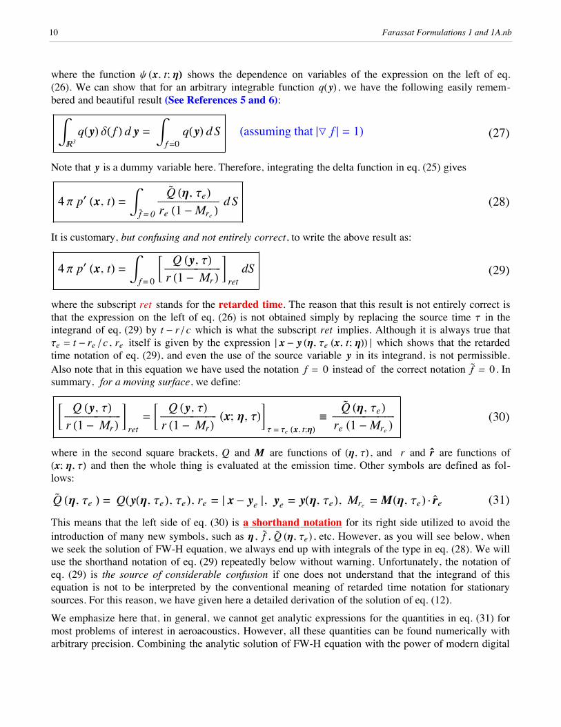
where the function y Hx, t; hL shows the dependence on variables of the expression on the left of eq.(26). We can show that for an arbitrary integrable function qHyL , we have the following easily remem-bered and beautiful result (See References 5 and 6):

(27)‡!3

qHyL dH f L d y = ‡f =0

qHyL d S Hassuming that †ı f § = 1L

Note that y is a dummy variable here. Therefore, integrating the delta function in eq. (25) gives

(28)4 p p£ Hx, tL = ‡fè

= 0

Qè

Hh, teLÅÅÅÅÅÅÅÅÅÅÅÅÅÅÅÅÅÅÅÅÅÅÅÅÅÅÅÅÅÅÅÅÅre H1 - Mre L d S

It is customary, but confusing and not entirely correct, to write the above result as:

(29)4 p p£ Hx, tL = ‡f = 0

C Q Hy, tLÅÅÅÅÅÅÅÅÅÅÅÅÅÅÅÅÅÅÅÅÅÅÅÅÅÅÅÅÅÅr H1 - MrL G ret

dS

where the subscript ret stands for the retarded time. The reason that this result is not entirely correct isthat the expression on the left of eq. (26) is not obtained simply by replacing the source time t in theintegrand of eq. (29) by t - r ê c which is what the subscript ret implies. Although it is always true thatte = t - re ê c , re itself is given by the expression † x - y Hh, te Hx, t; hLL § which shows that the retardedtime notation of eq. (29), and even the use of the source variable y in its integrand, is not permissible.Also note that in this equation we have used the notation f = 0 instead of the correct notation f

è= 0. In

summary, for a moving surface, we define:

(30)C Q Hy, tLÅÅÅÅÅÅÅÅÅÅÅÅÅÅÅÅÅÅÅÅÅÅÅÅÅÅÅÅÅÅr H1 - MrL G ret

= C Q Hy, tLÅÅÅÅÅÅÅÅÅÅÅÅÅÅÅÅÅÅÅÅÅÅÅÅÅÅÅÅÅÅr H1 - MrL Hx; h, tLG

t = te Hx, t;hLª

Qè

Hh, teLÅÅÅÅÅÅÅÅÅÅÅÅÅÅÅÅÅÅÅÅÅÅÅÅÅÅÅÅÅÅÅÅÅre H1 - Mre L

where in the second square brackets, Q and M are functions of Hh, tL , and r and r̀ are functions ofHx; h, tL and then the whole thing is evaluated at the emission time. Other symbols are defined as fol-lows:

(31)Qè

Hh, te L = QHyHh, teL, teL, re = † x - ye §, ye = yHh, teL, Mre = MHh, teL ÿ r̀e

This means that the left side of eq. (30) is a shorthand notation for its right side utilized to avoid theintroduction of many new symbols, such as h , f

è, Q

è Hh, teL , etc. However, as you will see below, when

we seek the solution of FW-H equation, we always end up with integrals of the type in eq. (28). We willuse the shorthand notation of eq. (29) repeatedly below without warning. Unfortunately, the notation ofeq. (29) is the source of considerable confusion if one does not understand that the integrand of thisequation is not to be interpreted by the conventional meaning of retarded time notation for stationarysources. For this reason, we have given here a detailed derivation of the solution of eq. (12).

We emphasize here that, in general, we cannot get analytic expressions for the quantities in eq. (31) formost problems of interest in aeroacoustics. However, all these quantities can be found numerically witharbitrary precision. Combining the analytic solution of FW-H equation with the power of modern digitalcomputers allows us to use the exact geometry and kinematics of rotating blade machinery. Thisapproach has been enormously successful in all areas of aeroacoustics.


We emphasize here that, in general, we cannot get analytic expressions for the quantities in eq. (31) formost problems of interest in aeroacoustics. However, all these quantities can be found numerically witharbitrary precision. Combining the analytic solution of FW-H equation with the power of modern digitalcomputers allows us to use the exact geometry and kinematics of rotating blade machinery. Thisapproach has been enormously successful in all areas of aeroacoustics.

Remark 4- When a source moves rectilinearly at uniform speed, then the source time can be found inclosed form by solving eq. (22). Furthermore, we discover that we have one emission time for subsonicmotion and two emission times for supersonic motion of the source. (End of Remark 4)

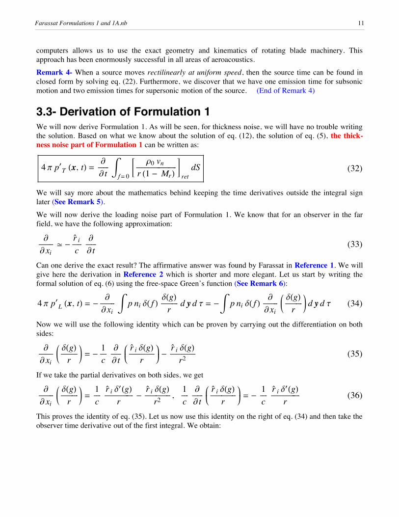
3.3- Derivation of Formulation 1We will now derive Formulation 1. As will be seen, for thickness noise, we will have no trouble writingthe solution. Based on what we know about the solution of eq. (12), the solution of eq. (5), the thick-ness noise part of Formulation 1 can be written as:

(32)4 p p£T Hx, tL =

ÅÅÅÅÅÅÅÅ t

‡f = 0

C r0 vnÅÅÅÅÅÅÅÅÅÅÅÅÅÅÅÅÅÅÅÅÅÅÅÅÅÅÅÅÅÅr H1 - MrL G ret

dS

We will say more about the mathematics behind keeping the time derivatives outside the integral signlater (See Remark 5).

We will now derive the loading noise part of Formulation 1. We know that for an observer in the farfield, we have the following approximation:

(33)


> -r̀ iÅÅÅÅÅÅÅc

ÅÅÅÅÅÅÅÅ t

Can one derive the exact result? The affirmative answer was found by Farassat in Reference 1. We willgive here the derivation in Reference 2 which is shorter and more elegant. Let us start by writing theformal solution of eq. (6) using the free-space Green’s function (See Remark 6):

(34)4 p p£L Hx, tL = -

ÅÅÅÅÅÅÅÅÅÅÅxi

‡ p ni dH f L dHgLÅÅÅÅÅÅÅÅÅÅÅÅÅ

r d y d t = -‡ p ni dH f L


K dHgLÅÅÅÅÅÅÅÅÅÅÅÅÅ

rO d y d t

Now we will use the following identity which can be proven by carrying out the differentiation on bothsides:

(35)



rO = -

1ÅÅÅÅÅc

ÅÅÅÅÅÅÅÅ t

ikjj r̀ i dHgLÅÅÅÅÅÅÅÅÅÅÅÅÅÅÅÅÅÅÅ

ry{zz -

r̀ i dHgLÅÅÅÅÅÅÅÅÅÅÅÅÅÅÅÅÅÅÅr2

If we take the partial derivatives on both sides, we get

(36)



rO =

1ÅÅÅÅÅc

r̀ i d£HgLÅÅÅÅÅÅÅÅÅÅÅÅÅÅÅÅÅÅÅÅÅ

r-

r̀ i dHgLÅÅÅÅÅÅÅÅÅÅÅÅÅÅÅÅÅÅÅr2 ,

1ÅÅÅÅÅc

ÅÅÅÅÅÅÅÅ t


ry{zz = -

1ÅÅÅÅÅc

r̀ i d£HgLÅÅÅÅÅÅÅÅÅÅÅÅÅÅÅÅÅÅÅÅÅ

rThis proves the identity of eq. (35). Let us now use this identity on the right of eq. (34) and then take theobserver time derivative out of the first integral. We obtain:


(37)4 p p£

L Hx, tL =1ÅÅÅÅÅc

‡ p ni dH f L ÅÅÅÅÅÅÅÅ t


ry{zz d y d t + ‡ p ni r̀ i dH f L dHgL

ÅÅÅÅÅÅÅÅÅÅÅÅÅr2 d y d t =

1ÅÅÅÅÅc

ÅÅÅÅÅÅÅÅ t

‡ p ni r̀ i dH f L dHgLÅÅÅÅÅÅÅÅÅÅÅÅÅ

r d y d t + ‡ p ni r̀ i dH f L dHgL

ÅÅÅÅÅÅÅÅÅÅÅÅÅr2 d y d t

See Remark 6 about an important mathematical point in relation to this equation. Again using thesolution of eq. (12), we write the solution of eq. (6) which is the loading noise part of Formulation 1as:

(38)4 p p£L Hx, tL =

1ÅÅÅÅÅc

ÅÅÅÅÅÅÅÅ t

‡f = 0

C p cos qÅÅÅÅÅÅÅÅÅÅÅÅÅÅÅÅÅÅÅÅÅÅÅÅÅÅÅÅÅÅr H1 - MrL G ret

dS + ‡f = 0

C p cos qÅÅÅÅÅÅÅÅÅÅÅÅÅÅÅÅÅÅÅÅÅÅÅÅÅÅÅÅÅÅÅÅÅr2 H1 - MrL G ret

dS

where cos q = ni r̀ i , i.e., q is the local angle between normal to the surface and radiation direction r̀ atthe emission time.

Formulation 1 of Farassat is the sum of eqs. (32) and (38):

(39)4 p p£ Hx, tL = 4 p Hp£

T Hx, tL + p£L Hx, tLL =

ÅÅÅÅÅÅÅÅ t

‡f = 0

C r0 vnÅÅÅÅÅÅÅÅÅÅÅÅÅÅÅÅÅÅÅÅÅÅÅÅÅÅÅÅÅÅr H1 - MrL +

p cos qÅÅÅÅÅÅÅÅÅÅÅÅÅÅÅÅÅÅÅÅÅÅÅÅÅÅÅÅÅÅÅÅÅÅc r H1 - MrL G ret

dS + ‡f = 0


dS

The observer time differentiation of Formulation 1 is always taken numerically in the applications ofthis result.

Remark 5- The solution of the wave equation with derivatives acting on the inhomoge-neous source termEquations (5) and (6) are of the following types:

(40)·2 f =qÅÅÅÅÅÅÅÅÅ t

and ·2 fi =q


Ix e !3, q differentiable in x and tMLet us consider the first equation. Assume that we find the solution of the following wave equation:

(41)·2 y = q

Then, by taking the time derivatives of both sides of eq. (41), we have the following result:

(42)ÅÅÅÅÅÅÅÅ t

·2 y = ·2 yÅÅÅÅÅÅÅÅÅÅ t

=qÅÅÅÅÅÅÅÅÅ t

Comparing this equation with the first wave equation in eq. (40), we have

(43)f Hx, tL =y Hx, tLÅÅÅÅÅÅÅÅÅÅÅÅÅÅÅÅÅÅÅÅÅÅÅÅÅ

tThis is the result we used in writing down eq. (32). Similarly, we have


(44)


·2 y = ·2 yÅÅÅÅÅÅÅÅÅÅÅxi

=q


When this result is compared with the second wave equation in eq. (40), we conclude that

(45)fi Hx, tL =y Hx, tLÅÅÅÅÅÅÅÅÅÅÅÅÅÅÅÅÅÅÅÅÅÅÅÅÅ

xi

This is the result used in eq. (34).

We make two further important comments here. First deriving the results in eqs. (43) and (45) using theGreen’s function solution of the wave equations of eq. (40) in the integral form as it is often done inbooks and technical journals, is difficult and involves much more algebraic manipulations. Second, ifwe relax the differentiability of the source function qHx, tL in eq. (40), then the results expressed by eqs.(43) and (45) are valid if all the derivatives ê t and ê xi on the right sides of eqs. (40), (43), and(45) are treated as generalized derivatives (See References 5 and 6). In fact, it is always more conve-nient to work in the space of generalized functions because of their powerful operational properties(ease of exchanging limit processes without worrying about differentiability, etc.). As a matter of fact, inmany practical problems, differentiability or even the continuity of the source term cannot be guaran-teed. However, using generalized functions can overcome most, if not all, the mathematical ambiguitiesand difficulties. (End of Remark 5)

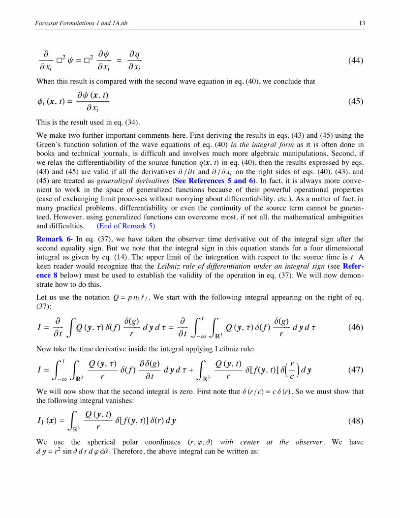
Remark 6- In eq. (37), we have taken the observer time derivative out of the integral sign after thesecond equality sign. But we note that the integral sign in this equation stands for a four dimensionalintegral as given by eq. (14). The upper limit of the integration with respect to the source time is t . Akeen reader would recognize that the Leibniz rule of differentiation under an integral sign (see Refer-ence 8 below) must be used to establish the validity of the operation in eq. (37). We will now demon-strate how to do this.

Let us use the notation Q = p ni r̀ i . We start with the following integral appearing on the right of eq.(37):

(46)I =

ÅÅÅÅÅÅÅÅ t

‡ Q Hy, tL dH f L dHgLÅÅÅÅÅÅÅÅÅÅÅÅÅ

r d y d t =

ÅÅÅÅÅÅÅÅ t

‡-¶

t ‡

!3 Q Hy, tL dH f L dHgL


d y d t

Now take the time derivative inside the integral applying Leibniz rule:

(47)I = ‡-¶

t ‡

!3 Q Hy, tLÅÅÅÅÅÅÅÅÅÅÅÅÅÅÅÅÅÅÅÅÅÅÅ

rdH f L dHgL

ÅÅÅÅÅÅÅÅÅÅÅÅÅÅÅÅÅ t

d y d t + ‡!3

Q Hy, tLÅÅÅÅÅÅÅÅÅÅÅÅÅÅÅÅÅÅÅÅÅ

rd@ f Hy, tLD dJ r

ÅÅÅÅÅcN d y

We will now show that the second integral is zero. First note that d Hr ê cL = c d HrL . So we must show thatthe following integral vanishes:

(48)I1 HxL = ‡!3

Q Hy, tLÅÅÅÅÅÅÅÅÅÅÅÅÅÅÅÅÅÅÅÅÅ

rd@ f Hy, tLD dHrL d y

We use the spherical polar coordinates Hr, j, JL with center at the observer. We haved y = r2 sin J d r d j dJ . Therefore, the above integral can be written as:


(49)I1 HxL = lim Ø 0‡0

p

‡0

2 p

‡0

¶

Q Hy, tL d@ f Hy, tLD r sin J dHr - L d r d j d J = 0

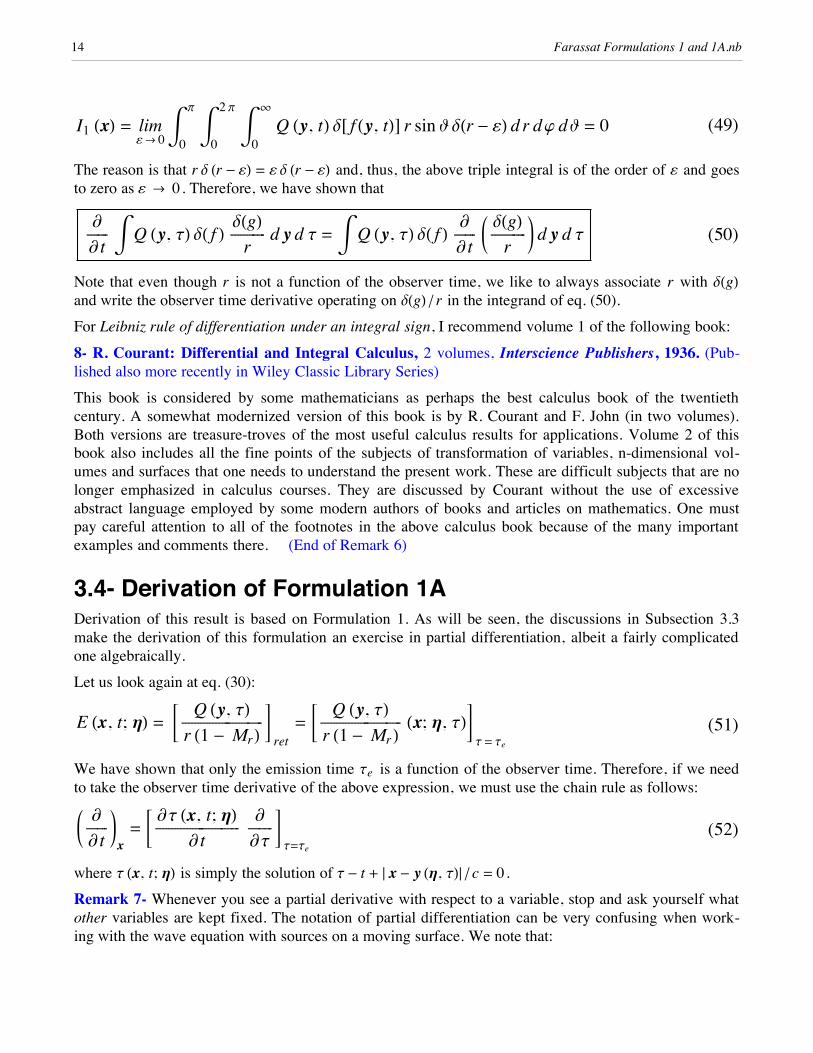
The reason is that r d Hr - L = d Hr - L and, thus, the above triple integral is of the order of and goesto zero as Ø 0. Therefore, we have shown that

(50)

ÅÅÅÅÅÅÅÅ t

‡ Q Hy, tL dH f L dHgLÅÅÅÅÅÅÅÅÅÅÅÅÅ

r d y d t = ‡ Q Hy, tL dH f L ÅÅÅÅÅÅÅÅ

t K dHgL


O d y d t

Note that even though r is not a function of the observer time, we like to always associate r with dHgLand write the observer time derivative operating on dHgL ê r in the integrand of eq. (50).

For Leibniz rule of differentiation under an integral sign, I recommend volume 1 of the following book:

8- R. Courant: Differential and Integral Calculus, 2 volumes, Interscience Publishers, 1936. (Pub-lished also more recently in Wiley Classic Library Series)

This book is considered by some mathematicians as perhaps the best calculus book of the twentiethcentury. A somewhat modernized version of this book is by R. Courant and F. John (in two volumes).Both versions are treasure-troves of the most useful calculus results for applications. Volume 2 of thisbook also includes all the fine points of the subjects of transformation of variables, n-dimensional vol-umes and surfaces that one needs to understand the present work. These are difficult subjects that are nolonger emphasized in calculus courses. They are discussed by Courant without the use of excessiveabstract language employed by some modern authors of books and articles on mathematics. One mustpay careful attention to all of the footnotes in the above calculus book because of the many importantexamples and comments there. (End of Remark 6)

3.4- Derivation of Formulation 1ADerivation of this result is based on Formulation 1. As will be seen, the discussions in Subsection 3.3make the derivation of this formulation an exercise in partial differentiation, albeit a fairly complicatedone algebraically.

Let us look again at eq. (30):

(51)E Hx, t; hL = C Q Hy, tLÅÅÅÅÅÅÅÅÅÅÅÅÅÅÅÅÅÅÅÅÅÅÅÅÅÅÅÅÅÅr H1 - MrL G ret

= C Q Hy, tLÅÅÅÅÅÅÅÅÅÅÅÅÅÅÅÅÅÅÅÅÅÅÅÅÅÅÅÅÅÅr H1 - MrL Hx; h, tLG

t = te

We have shown that only the emission time te is a function of the observer time. Therefore, if we needto take the observer time derivative of the above expression, we must use the chain rule as follows:

(52)K ÅÅÅÅÅÅÅÅ t

Ox

= C t Hx, t; hLÅÅÅÅÅÅÅÅÅÅÅÅÅÅÅÅÅÅÅÅÅÅÅÅÅÅÅÅÅÅÅ

t

ÅÅÅÅÅÅÅÅÅt

Gt=te

where t Hx, t; hL is simply the solution of t - t + † x - y Hh, tL§ ê c = 0.

Remark 7- Whenever you see a partial derivative with respect to a variable, stop and ask yourself whatother variables are kept fixed. The notation of partial differentiation can be very confusing when work-ing with the wave equation with sources on a moving surface. We note that:

1- In deriving this equation, we assume that the moving surface f = 0 is defined in a Lagrangian frameh fixed to the surface. This frame is also called the blade-fixed frame. We have y = y Hh, tL , so thatr = r H x, y Hh, tLL . Also note that the surface integration is most conveniently carried out in the h-frame,i.e., we are really integrating over the surface f

è HhL = 0.


1- In deriving this equation, we assume that the moving surface f = 0 is defined in a Lagrangian frameh fixed to the surface. This frame is also called the blade-fixed frame. We have y = y Hh, tL , so thatr = r H x, y Hh, tLL . Also note that the surface integration is most conveniently carried out in the h-frame,i.e., we are really integrating over the surface f

è HhL = 0.

2- We have also shown that the emission time is analytically written as follows t = te Hx, t; hL althoughwe cannot find this function explicitly for rotating blades.

Therefore, in partial differentiation of the left side of eq. (52), we are keeping the variables Hx, hL fixed.All these also mean that we need to find te ê t on the right side of eq. (52) keeping the variables Hx, hLfixed. (End of Remark 7)

Now we find t ê t . We have shown above that the emission time satisfies the following equation:

(53)g = t - t + r H x, y Hh, tLL ê c = 0where h is a given fixed point on the moving surface. By taking partial derivative with respect to t ofeq. (53), we get

(54)K tÅÅÅÅÅÅÅÅÅ t

OHx, hL

- 1 +1ÅÅÅÅÅc

K rÅÅÅÅÅÅÅÅÅ t

OHx, hL

= K teÅÅÅÅÅÅÅÅÅÅÅÅ t

OHx, hL

- 1 - M r K tÅÅÅÅÅÅÅÅÅ t

OHx, hL

= 0

where M r is the Mach number of the point h in the radiation direction at the time t . Here we have usedthe following relations:

(55)K rÅÅÅÅÅÅÅÅÅ t

OHx, hL

= K rÅÅÅÅÅÅÅÅÅt

OHx, hL

K tÅÅÅÅÅÅÅÅÅ t

OHx, hL

(56)K rÅÅÅÅÅÅÅÅÅt

OHx, hL

=r

ÅÅÅÅÅÅÅÅÅÅÅ yi

ikjj yiÅÅÅÅÅÅÅÅÅÅÅt

y{zzHx, hL

= - r̀i vi = - vr

where r̀i is the component of unit radiation vector and vr is the velocity of the point h in the radiationdirection.

From eqs. (54-56), we find

(57)K tÅÅÅÅÅÅÅÅÅ t

OHx, hL

=1

ÅÅÅÅÅÅÅÅÅÅÅÅÅÅÅÅÅÅÅÅÅ1 - M r

This result leads to the following important formula:

(58)

ÅÅÅÅÅÅÅÅ t

@qHx, y, tLDret

=

ÅÅÅÅÅÅÅÅ t

@qHx, y Hh, tL, te Hx, t; hLLD = C 1ÅÅÅÅÅÅÅÅÅÅÅÅÅÅÅÅÅÅÅÅÅ1 - M r

qHx, y, tLÅÅÅÅÅÅÅÅÅÅÅÅÅÅÅÅÅÅÅÅÅÅÅÅÅÅÅÅÅÅÅ

tG

ret

We warn the readers once more that the right side of eq. (58) is a shorthand notation which must beinterpreted as:


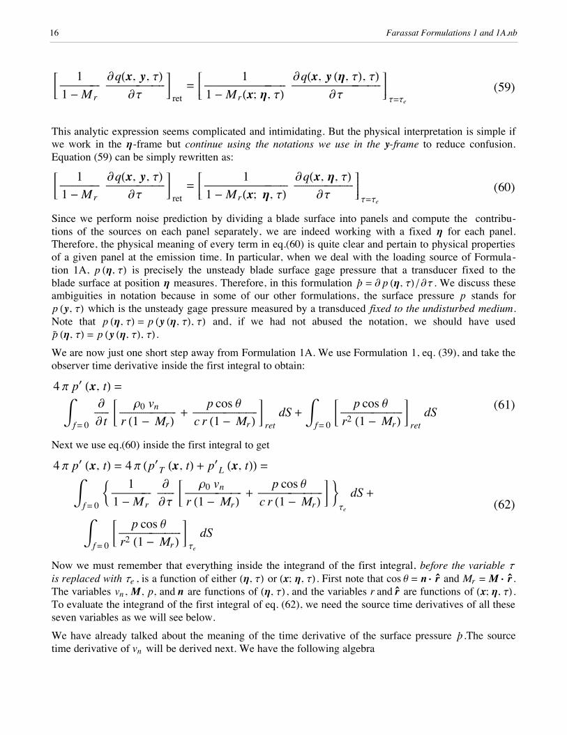
(59)C 1ÅÅÅÅÅÅÅÅÅÅÅÅÅÅÅÅÅÅÅÅÅ1 - M r


tG

ret=ÄÇÅÅÅÅÅÅÅ

1ÅÅÅÅÅÅÅÅÅÅÅÅÅÅÅÅÅÅÅÅÅÅÅÅÅÅÅÅÅÅÅÅÅÅÅÅÅÅÅÅÅÅÅ1 - M rHx; h, tL

qHx, y Hh, tL, tLÅÅÅÅÅÅÅÅÅÅÅÅÅÅÅÅÅÅÅÅÅÅÅÅÅÅÅÅÅÅÅÅÅÅÅÅÅÅÅÅÅÅÅÅÅÅÅ

t

ÉÖÑÑÑÑÑÑÑ t=te

This analytic expression seems complicated and intimidating. But the physical interpretation is simple ifwe work in the h-frame but continue using the notations we use in the y-frame to reduce confusion.Equation (59) can be simply rewritten as:

(60)C 1ÅÅÅÅÅÅÅÅÅÅÅÅÅÅÅÅÅÅÅÅÅ1 - M r


tG

ret=ÄÇÅÅÅÅÅÅÅ

1ÅÅÅÅÅÅÅÅÅÅÅÅÅÅÅÅÅÅÅÅÅÅÅÅÅÅÅÅÅÅÅÅÅÅÅÅÅÅÅÅÅÅÅÅ1 - M rHx; h, tL

qHx, h, tLÅÅÅÅÅÅÅÅÅÅÅÅÅÅÅÅÅÅÅÅÅÅÅÅÅÅÅÅÅÅÅ

t

ÉÖÑÑÑÑÑÑÑ t=te

Since we perform noise prediction by dividing a blade surface into panels and compute the contribu-tions of the sources on each panel separately, we are indeed working with a fixed h for each panel.Therefore, the physical meaning of every term in eq.(60) is quite clear and pertain to physical propertiesof a given panel at the emission time. In particular, when we deal with the loading source of Formula-tion 1A, p Hh, tL is precisely the unsteady blade surface gage pressure that a transducer fixed to theblade surface at position h measures. Therefore, in this formulation p° = p Hh, tL êt . We discuss theseambiguities in notation because in some of our other formulations, the surface pressure p stands forp Hy, tL which is the unsteady gage pressure measured by a transduced fixed to the undisturbed medium.Note that p Hh, tL = p Hy Hh, tL, tL and, if we had not abused the notation, we should have usedpè Hh, tL = p Hy Hh, tL, tL . We are now just one short step away from Formulation 1A. We use Formulation 1, eq. (39), and take theobserver time derivative inside the first integral to obtain:

(61)4 p p£ Hx, tL =

‡f = 0

ÅÅÅÅÅÅÅÅ t


p cos qÅÅÅÅÅÅÅÅÅÅÅÅÅÅÅÅÅÅÅÅÅÅÅÅÅÅÅÅÅÅÅÅÅÅc r H1 - MrL G ret

dS + ‡f = 0


dS

Next we use eq.(60) inside the first integral to get

(62)

4 p p£ Hx, tL = 4 p Hp£T Hx, tL + p£

L Hx, tLL =

‡f = 0

; 1ÅÅÅÅÅÅÅÅÅÅÅÅÅÅÅÅÅÅÅÅÅ1 - M r

ÅÅÅÅÅÅÅÅÅt


p cos qÅÅÅÅÅÅÅÅÅÅÅÅÅÅÅÅÅÅÅÅÅÅÅÅÅÅÅÅÅÅÅÅÅÅc r H1 - MrL G ?te

dS +

‡f = 0

C p cos qÅÅÅÅÅÅÅÅÅÅÅÅÅÅÅÅÅÅÅÅÅÅÅÅÅÅÅÅÅÅÅÅÅr2 H1 - MrL G te

dS

Now we must remember that everything inside the integrand of the first integral, before the variable tis replaced with te , is a function of either Hh, tL or Hx; h, tL . First note that cos q = n r̀ and Mr = M r̀ .The variables vn , M, p, and n are functions of Hh, tL , and the variables r and r̀ are functions of Hx; h, tL .To evaluate the integrand of the first integral of eq. (62), we need the source time derivatives of all theseseven variables as we will see below.

We have already talked about the meaning of the time derivative of the surface pressure p† .The sourcetime derivative of vn will be derived next. We have the following algebra


(63)v† n ª

ÅÅÅÅÅÅÅÅÅt

Hv nL = v† n + v n† = an + v wän

where a = v† = v êt = c M†

is the acceleration of the point h and w is the angular velocity of the bladesurface. Note that, in general, v wän 0 on a blade. We can now easily show the following results:

(64)rÅÅÅÅÅÅÅÅÅt

=r

ÅÅÅÅÅÅÅÅÅÅÅyi

yi Hh, tLÅÅÅÅÅÅÅÅÅÅÅÅÅÅÅÅÅÅÅÅÅÅÅÅÅÅÅ

t= - r̀ v = vr

(65) r̀iÅÅÅÅÅÅÅÅÅÅt

=r̀i vr - viÅÅÅÅÅÅÅÅÅÅÅÅÅÅÅÅÅÅÅÅÅÅÅÅÅ

r

(66)MrÅÅÅÅÅÅÅÅÅÅÅÅÅÅt

=1

ÅÅÅÅÅÅÅÅÅc r

Iri v† i + vr2 - v2M = r̀i M

†i +

c IMr2 - M2M

ÅÅÅÅÅÅÅÅÅÅÅÅÅÅÅÅÅÅÅÅÅÅÅÅÅÅÅÅÅÅÅÅÅÅÅÅr

We can next perform the tedious source time differentiation in eq.(62) and utilize the above results inthe algebra. Here we separate the thickness and loading noise results as in Reference 4. The Thick-ness and Loading noise components of Formulation 1A is

(67)

4 p p£T Hx, tL =

‡f = 0

ÄÇÅÅÅÅÅÅÅÅÅ

r0 v† nÅÅÅÅÅÅÅÅÅÅÅÅÅÅÅÅÅÅÅÅÅÅÅÅÅÅÅÅÅÅÅr H1 - MrL2

+r0 vn r̀i M

†iÅÅÅÅÅÅÅÅÅÅÅÅÅÅÅÅÅÅÅÅÅÅÅÅÅÅÅÅÅÅÅ

r H1 - MrL3ÉÖÑÑÑÑÑÑÑÑÑret

d S + ‡f = 0

Ä

ÇÅÅÅÅÅÅÅÅÅ

r0 c vn IMr - M2MÅÅÅÅÅÅÅÅÅÅÅÅÅÅÅÅÅÅÅÅÅÅÅÅÅÅÅÅÅÅÅÅÅÅÅÅÅÅÅÅÅÅÅÅÅÅÅÅÅÅ

r2 H1 - MrL3É

ÖÑÑÑÑÑÑÑÑÑret

d S

(68)

4 p p£L Hx, tL = ‡

f = 0 ÄÇÅÅÅÅÅÅÅÅÅ

p† cos qÅÅÅÅÅÅÅÅÅÅÅÅÅÅÅÅÅÅÅÅÅÅÅÅÅÅÅÅÅÅÅÅÅÅÅÅc r H1 - MrL2

+r̀i M

†i p cos q

ÅÅÅÅÅÅÅÅÅÅÅÅÅÅÅÅÅÅÅÅÅÅÅÅÅÅÅÅÅÅÅÅÅÅÅÅc r H1 - MrL3

ÉÖÑÑÑÑÑÑÑÑÑret

d S +

‡f = 0

Ä

ÇÅÅÅÅÅÅÅÅÅ

p Hcos q - Mi niLÅÅÅÅÅÅÅÅÅÅÅÅÅÅÅÅÅÅÅÅÅÅÅÅÅÅÅÅÅÅÅÅÅÅÅÅÅÅÅÅÅÅÅÅÅÅr2 H1 - MrL2

+IMr - M2M p cos q

ÅÅÅÅÅÅÅÅÅÅÅÅÅÅÅÅÅÅÅÅÅÅÅÅÅÅÅÅÅÅÅÅÅÅÅÅÅÅÅÅÅÅÅÅÅÅÅÅÅÅÅr2 H1 - MrL3

É

ÖÑÑÑÑÑÑÑÑÑret

d S

We have written these equations differently from those in Reference 4 by separating the near fieldterms (order 1 ë r2 ) from the far field terms (order 1 ê r ). We have left out much algebraic manipula-tions in obtaining the above results. The derivation of Formulation 1A has been checked many times byacoustic researchers. We mention here that although the combination of variables Mr

2 - M2 appears ineq.(66), the appearance of the combination of variables Mr - M2 in eqs.(67) and (68) is correct.

Remark 8- The loading noise part of Formulation 1A can be derived in other ways. For example, wehave


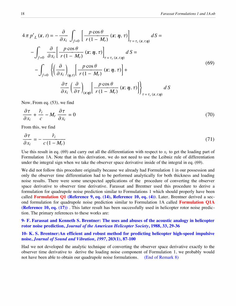
(69)

4 p p£L Hx, tL = -


‡f =0

C p cos qÅÅÅÅÅÅÅÅÅÅÅÅÅÅÅÅÅÅÅÅÅÅÅÅÅÅÅÅÅÅÅr H1 - MrL Hx; h, tLG

t = te Hx, t;hL d S =

-‡f =0


C p cos qÅÅÅÅÅÅÅÅÅÅÅÅÅÅÅÅÅÅÅÅÅÅÅÅÅÅÅÅÅÅÅr H1 - MrL Hx; h, tLG

t = te Hx, t;hL d S =

-‡f =0

lomnoK


OHh,tL

C p cos qÅÅÅÅÅÅÅÅÅÅÅÅÅÅÅÅÅÅÅÅÅÅÅÅÅÅÅÅÅÅÅr H1 - MrL Hx; h, tLG +

tÅÅÅÅÅÅÅÅÅÅÅxi

K ÅÅÅÅÅÅÅÅÅt

OHx;hL

C p cos qÅÅÅÅÅÅÅÅÅÅÅÅÅÅÅÅÅÅÅÅÅÅÅÅÅÅÅÅÅÅÅr H1 - MrL Hx; h, tLG|o}

~ot = te Hx, t;hL d S

Now, From eq. (53), we find

(70)t


+r̀iÅÅÅÅÅÅc

- Mr t


= 0

From this, we find

(71)t


= -r̀iÅÅÅÅÅÅÅÅÅÅÅÅÅÅÅÅÅÅÅÅÅÅÅÅÅÅÅÅÅ

c H1 - MrLUse this result in eq. (69) and carry out all the differentiation with respect to xi to get the loading part ofFormulation 1A. Note that in this derivation, we do not need to use the Leibniz rule of differentiationunder the integral sign when we take the observer space derivative inside of the integral in eq. (69).

We did not follow this procedure originally because we already had Formulation 1 in our possession andonly the observer time differentiation had to be performed analytically for both thickness and loadingnoise results. There were some unexpected applications of the procedure of converting the observerspace derivative to observer time derivative. Farassat and Brentner used this procedure to derive aformulation for quadrupole noise prediction similar to Formulations 1 which should properly have beencalled Formulation Q1 (Reference 9, eq. (14), Reference 10, eq. (4)). Later, Brentner derived a sec-ond formulation for quadrupole noise prediction similar to Formulation 1A called Formulation Q1A(Reference 10, eq. (17)) . This latter result has been successfully used in helicopter rotor noise predic-tion. The primary references to these works are:

9- F. Farassat and Kenneth S. Brentner: The uses and abuses of the acoustic analogy in helicopterrotor noise prediction, Journal of the American Helicopter Society, 1988, 33, 29-3610- K. S. Brentner:An efficient and robust method for predicting helicopter high-speed impulsivenoise, Journal of Sound and Vibration, 1997, 203(1), 87-100 Had we not developed the analytic technique of converting the observer space derivative exactly to theobserver time derivative to derive the loading noise component of Formulation 1, we probably wouldnot have been able to obtain our quadrupole noise formulations. (End of Remark 8)


3.5- Moving ObserverIn most applications, we want to compute the noise in a frame moving with the aircraft, i.e., as measuredby a microphone attached to the aircraft. All propeller and helicopter rotor noise prediction codes atLangley Research Center have this capability. It is important to realize that the observer variable x inFormulations 1 and 1A is in the frame fixed to the medium. Let us attach a frame fixed to the aircraftwith axes parallel to the medium-fixed x-frame. We will call this X-frame. Assume that at the time t = 0the two frames coincide. Let the velocity of the aircraft be VHtL . Then the origin of the X-frame will beat the point

(72)X0HtL = ‡0

t VHt£L d t£

Now a point X in the X-frame will be at the point x = X + X0HtL at the time t . Therefore, if we want tofind the acoustic pressure pè £ HX, tL as a function of time in the X-frame from our formulations, we usethe following formula:

(73)pè £ HX, tL = p£ HX + X0HtL, tLThe interpretation of this result is simple. To calculate the acoustic pressure pè £ HX, tL in the aircraft fixedframe, make sure you compute first where the observer (or the microphone) is in the x-frame at the timet. Then use that observer position in the formulations given by eq. (73).

4- Concluding RemarksLangley Research Center researchers have been involved in the prediction of the noise of rotating bladessince the nineteen thirties. It was after the introduction of high speed digital computers in nineteensixties that it was possible to use realistic geometry and kinematics of the rotors and propellers in thenoise prediction process. The pace of aeroacoustic research increased since the early nineteen seventiesbecause of the public pressure to reduce aircraft noise particularly around airports. Both the govern-ments and the aircraft industry around the world realized that aeroacoustic research can lead to substan-tial aircraft noise reduction. The invention of high speed digital computers played a major role in thiseffort in the areas of aeroacoustic modeling, transducer design, data analysis, full scale flight and windtunnel tests. Advanced mathematics have played a vital role in all these areas although this fact is notmentioned often by the researchers.

In developing noise prediction models at Langley Research Center for propellers and helicopter rotors,we used primarily the acoustic analogy based the FW-H equation. We developed general solutions ofthis equation which allowed using realistic blade geometry and kinematics. We also did not want to belimited to problems that generated periodic acoustic waveforms. Finally, we required that our formula-tions be valid in both near and far fields. These conditions could be met if we worked in the timedomain and then applied a Fourier transform in time to obtain frequency domain results. This approachhas been very fruitful so far and is being followed by many other researchers around the world.

The current trend in aircraft noise prediction appears to be toward using FW-Hpds for all helicopter rotorand propeller noise prediction. This would make Formulation 1A even more useful in the future for allrotating blade noise prediction problems. For example, it makes sense to use this formulation for predict-ing supersonic propeller noise when an advanced unsteady aerodynamic code becomes available. This iswhat we are proposing at present for this problem.


The current trend in aircraft noise prediction appears to be toward using FW-Hpds for all helicopter rotorand propeller noise prediction. This would make Formulation 1A even more useful in the future for allrotating blade noise prediction problems. For example, it makes sense to use this formulation for predict-ing supersonic propeller noise when an advanced unsteady aerodynamic code becomes available. This iswhat we are proposing at present for this problem.

Now I would like to give some practical advice for developing a noise prediction code based on my ownexperience at Langley Research Center:

1- Always derive fully the acoustic formulation you want to use. This way you understand the exactmeaning of all the terms in the formulation as well as its subtleties, e.g., the fluid velocities are definedrelative to what frame. Also, it is possible that some misprints in the printed reference, such as a signerror, can cause serious errors in acoustic calculations.

2- Spend a lot of time designing the algorithms you want to use and studying the flow of information inthe code. This is the most important step in the reduction of computation time and it should be givenserious attention. We give some examples below:

– Use advanced surface integration techniques such as Gauss-Legendre integration .

– Emission time computation can be very time consuming on a computer. A well-designed algorithmhere is essential for an efficient code.

– Sometimes a do loop in the wrong place in the code can increase the computation time considerably.This is where the experience of the code developer becomes important.

3- Since we have derived exact results here, the readers should realize that in the near field the Fouriertransform of the computed acoustic pressure can have a large constant term. This term is negative on thesuction side of the rotor or propeller disc and positive on the pressure side as the physics of the problemwould dictate. This is confusing to a novice in the field of aeroacoustics because the measured resultsgenerally do not show this constant value (called DC shift by experimenters). Most commonly usedmicrophones cannot measure this shift. These microphones are said to be AC coupled and remove theDC shift.


REPORT DOCUMENTATION PAGE Form ApprovedOMB No. 0704-0188

2. REPORT TYPE Technical Memorandum

4. TITLE AND SUBTITLE

Derivation of Formulations 1 and 1A of Farassat

5a. CONTRACT NUMBER

6. AUTHOR(S)

F. Farassat

7. PERFORMING ORGANIZATION NAME(S) AND ADDRESS(ES)NASA Langley Research CenterHampton, VA 23681-2199

9. SPONSORING/MONITORING AGENCY NAME(S) AND ADDRESS(ES)National Aeronautics and Space AdministrationWashington, DC 20546-0001

8. PERFORMING ORGANIZATION REPORT NUMBER

L-19318

10. SPONSOR/MONITOR'S ACRONYM(S)

NASA

13. SUPPLEMENTARY NOTES

Lecture delivered to Aeroacoustics Branch staff on Monday, October 23, 2006.

12. DISTRIBUTION/AVAILABILITY STATEMENTUnclassified - UnlimitedSubject Category 71Availability: NASA CASI (301) 621-0390

19a. NAME OF RESPONSIBLE PERSONSTI Help Desk (email: [email protected])

14. ABSTRACTFormulations 1 and 1A are the solutions of the Ffowcs Williams-Hawkings (FW-H) equation with surface sources only when the surface moves at subsonic speed. Both formulations have been successfully used for helicopter rotor and propeller noise prediction for many years although we now recommend using Formulation 1A for this purpose. Formulation 1 has an observer time derivative that is taken numerically, and thus, increasing execution time on a computer and reducing the accuracy of the results. After some discussion of the Green's function of the wave equation, we derive Formulation 1 which is the basis of deriving Formulation 1A. We will then show how to take this observer time derivative analytically to get Formulation 1A. We give here the most detailed derivation of these formulations. Once you see the whole derivation, you will ask yourself why you did not do it yourself!

15. SUBJECT TERMSAeroacoustics, Noise Prediction, Acoustic Analogy, Ffowcs Williams-Hawkings (FW-H) Equation, Wave Equation, Formulation 1 of Farassat, Formulation 1A of Farassat, Generalized Functions, Propeller Noise Prediction, Helicopter Rotor Noise Prediction

18. NUMBER OF PAGES

2519b. TELEPHONE NUMBER (Include area code)

(301) 621-0390

a. REPORT

U

c. THIS PAGE

U

b. ABSTRACT

U

17. LIMITATION OF ABSTRACT

UU

Prescribed by ANSI Std. Z39.18Standard Form 298 (Rev. 8-98)

3. DATES COVERED (From - To)

5b. GRANT NUMBER

5c. PROGRAM ELEMENT NUMBER

5d. PROJECT NUMBER

5e. TASK NUMBER

5f. WORK UNIT NUMBER

561581.02.07.07

11. SPONSOR/MONITOR'S REPORT NUMBER(S)

NASA/TM-2007-214853

16. SECURITY CLASSIFICATION OF:

The public reporting burden for this collection of information is estimated to average 1 hour per response, including the time for reviewing instructions, searching existing data sources, gathering and maintaining the data needed, and completing and reviewing the collection of information. Send comments regarding this burden estimate or any other aspect of this collection of information, including suggestions for reducing this burden, to Department of Defense, Washington Headquarters Services, Directorate for Information Operations and Reports (0704-0188), 1215 Jefferson Davis Highway, Suite 1204, Arlington, VA 22202-4302. Respondents should be aware that notwithstanding any other provision of law, no person shall be subject to any penalty for failing to comply with a collection of information if it does not display a currently valid OMB control number.PLEASE DO NOT RETURN YOUR FORM TO THE ABOVE ADDRESS.

1. REPORT DATE (DD-MM-YYYY)03 - 200701-

Derivation of Formulations 1 and 1A of Farassat - NASA · • TECHNICAL TRANSLATION. English- ......

Documents

Transcript of Derivation of Formulations 1 and 1A of Farassat - NASA · • TECHNICAL TRANSLATION. English- ......