Int J Comput VisDOI 10.1007/s11263-017-1025-7

Depth Sensing Using Geometrically Constrained PolarizationNormals

Achuta Kadambi1 · Vage Taamazyan1,2,3 · Boxin Shi1,4 · Ramesh Raskar1

Received: 10 May 2016 / Accepted: 31 May 2017© Springer Science+Business Media, LLC 2017

Abstract Analyzing the polarimetric properties of reflectedlight is a potential source of shape information. However, itis well-known that polarimetric information contains fun-damental shape ambiguities, leading to an underconstrainedproblem of recovering 3D geometry. To address this prob-lem, we use additional geometric information, from coarsedepth maps, to constrain the shape information from polar-ization cues. Our main contribution is a framework thatcombines surface normals frompolarization (hereafter polar-ization normals) with an aligned depth map. The additionalgeometric constraints are used tomitigate physics-based arti-facts, such as azimuthal ambiguity, refractive distortion andfronto-parallel signal degradation. We believe our work mayhave practical implications for optical engineering, demon-strating a new option for state-of-the-art 3D reconstruction.

Communicated by Rene Vidal, Katsushi Ikeuchi, Josef Sivic andChristoph Schnoerr.

B Achuta Kadambiachoo@mit.edu

B Boxin Shishiboxin@media.mit.edu; boxin.shi@aist.go.jp

Vage Taamazyanvaheta@gmail.com; vaheta@tardis3d.ru

Ramesh Raskarraskar@media.mit.edu

1 MIT Media Lab, 75 Amherst Street, Cambridge, MA 02139,USA

2 Skoltech-MIT Initiative, Moscow Institute of Physics andTechnology, Moscow, Russia

3 Tardis 3D Technologies LLC, Moscow, Russia

4 Artificial Intelligence Research Center, National Institute ofAdvanced Industrial Science and Technology (AIST), Tokyo,Japan

Keywords Computational photography · Light transport ·Depth sensing · Shape from polarization

1 Introduction

Today, photographers use polarizing filters on 2D camerasto create aesthetic photographs. But what if a polarizing filteris used in the context of 3D photography? In the vein ofcomputational imaging, we present a co-design of polarizedoptics andpost-capture processing for the taskof 3D imaging.

Currently, consumer 3Dcameras like theMicrosoftKinectproduce depth maps that are often noisy and lack sufficientdetail. Using computational processing alone is unlikely tomitigate the problem (e.g., if the noise is filtered, so is thedetail). As such, there is recent interest in using a jointoptical and computational approach to both enhance detailand remove noise. One of the most promising solutions isto combine the captured, coarse depth map with surfacenormals obtained from photometric stereo (PS) or shape-from-shading (SfS). This depth-normal fusion is logical—thecoarse depth map provides the geometric structure and thesurface normals capture fine detail to be fused. Encourag-ing results have been shown by several papers that combinelow-quality depth maps with surface normal maps obtainedfrom SfS or PS.1 Unfortunately, SfS and PS are limited bysimilar scene assumptions, e.g., restrictive lighting andmate-rial assumptions. As a complementary technique, this paperproposes the first use of surface normals from polarizationto enhance depth maps. While our proposed technique alsohas assumptions on lighting and material properties, these

1 For example, (Yu et al. 2013; Han et al. 2013; Wu et al. 2014) usingSfS, and (Nehab et al. 2005; Haque et al. 2014) using PS.

123

Int J Comput Vis

(a) (b) (c) (d) (e)Input: Polarization Photos Result after Section 4.1.2Input: Kinect Only Result after Section 3.1 Result after Section 4.2

Coarse depth to correctazimuthal ambiguity artifacts

Canon T3i DSLRHoya CIR-PL FilterMicrosoft Kinect Version II Correcting refractive distortion

and physics-based integrationShape from Polarization

Fig. 1 Outline of proposed technique. a The Kinect depth of an objectis combined with (b) three photos at different rotations of a polarizingfilter. c Integration of surface normals obtained from Fresnel equations.Note the azimuthal ambiguity (observed as aflip in the shape) and distor-

tion of the zenith angle (observed as flatness in the shape). d Integrationof surface normals after correcting for azimuthal ambiguity removesthe flip, and the final result is shown in (e) after correcting for zenithdistortion and using physics-based integration

assumptions work on new types of scenes that PS and SfScannot handle.

For over a century it has been known that the shape of anobject causes small changes in the polarization of reflectedlight, best visualized by rotating a polarizing filter in front ofa digital camera.2 If properly constrained, obtaining shapethrough polarization has potential advantages over SfS andPS, including:

– Passive capture: assuming light incident on an object isunpolarized, the surface normals can be obtainedby rotat-ing a polarizer at the imaging sensor.

– Robustness to diffuse interreflections: unlike SfS and PS,diffuse interreflections do not significantly corrupt theestimated shape.

– Material invariant capture: the physics of the shape frompolarization problem hold for materials ranging fromdielectrics to metals to translucent objects.

– Lighting robust capture: if the incident light is unpolar-ized shape estimation is robust and can be conductedindoors, outdoors, or under patterned illumination.

However, there appears to be untapped potential as obtain-ing surface normals through polarization is not yet a maturetechnique. The obtained normals are drastically distorted.Specific open problems (Mitra and Nguyen 2003; Atkinsonand Hancock 2006) include:

1. Ambiguity The azimuth component of the surface nor-mal contains an ambiguity of π radians, which leads toambiguous flips in the 3D shape.

2. Refractive distortion Obtaining the zenith component ofthe surface normal requires knowledge of the refractiveindex to estimate accurate 3D shape.

3. Fronto-parallel surfaces When the zenith angle is closeto zero, the obtained normals are noisy.

2 Formalized by Augustin-Jean Fresnel (1788–1827) as the famous“Fresnel Equations”.

4. Depth discontinuities Even if the normals are obtainedcorrectly, integration of gradients must be performed torecover the 3D shape.

5. Relative depth Integrating surface normals obtains onlyrelative 3D shape, up to offset and scaling constants.

We believe that a solution to the above 5 problems is a sig-nificant step toward practical depth sensing. Although thereare partial solutions in prior art, that address restricted cases,a comprehensive solution to the above 5 problems has notbeen presented. In this paper, the 5 challenges are addressedby starting with a coarse depth map as a constraint to cor-rect the normals obtained from polarization.While we do notsolve all open problems, our correction is sufficient to realizeearly-stage practical results and hopefully spur future work.An overview of our approach is summarized in Fig. 1.

A preliminary version of this work was demonstrated liveat SIGGRAPH in August 2015 (Kadambi et al. 2015b) andappeared at ICCV inDecember 2015 (Kadambi et al. 2015a).This paper includes additional material pertaining to: atheoretical analysis of mixed reflections based on wave inter-ference (Sect. 5.1), a practical analysis of the unpolarizedworld assumption (Sect. 5.2), additional results including afailure case and demonstration using a laser scanner, andfinally expansions to the prose and discussion of relatedworks.

1.1 Contributions

Conceptually, we propose a technique that exploits surfacenormals from polarization cues to enhance the quality of acoarse depth map. This is the first technique that uses a depthmap to address the fundamental ambiguities in SfP. Veryspecifically, we devise a physics-based framework, whereinthe coarse depth map is used to resolve azimuthal ambiguity(addressing problem 1) and correct for refractive distortion(solving problem 2). To recover 3D shape, we propose aspanning tree integration scheme that uses the degree of

123

Int J Comput Vis

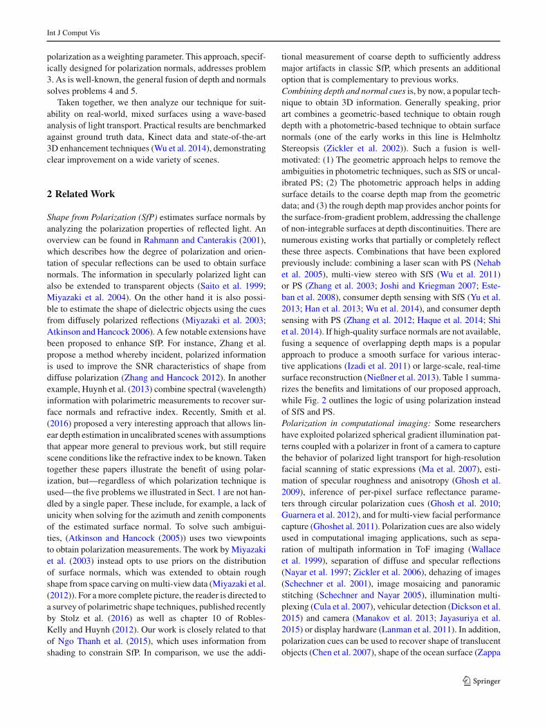
polarization as a weighting parameter. This approach, specif-ically designed for polarization normals, addresses problem3. As is well-known, the general fusion of depth and normalssolves problems 4 and 5.

Taken together, we then analyze our technique for suit-ability on real-world, mixed surfaces using a wave-basedanalysis of light transport. Practical results are benchmarkedagainst ground truth data, Kinect data and state-of-the-art3D enhancement techniques (Wu et al. 2014), demonstratingclear improvement on a wide variety of scenes.

2 Related Work

Shape from Polarization (SfP) estimates surface normals byanalyzing the polarization properties of reflected light. Anoverview can be found in Rahmann and Canterakis (2001),which describes how the degree of polarization and orien-tation of specular reflections can be used to obtain surfacenormals. The information in specularly polarized light canalso be extended to transparent objects (Saito et al. 1999;Miyazaki et al. 2004). On the other hand it is also possi-ble to estimate the shape of dielectric objects using the cuesfrom diffusely polarized reflections (Miyazaki et al. 2003;Atkinson and Hancock 2006). A few notable extensions havebeen proposed to enhance SfP. For instance, Zhang et al.propose a method whereby incident, polarized informationis used to improve the SNR characteristics of shape fromdiffuse polarization (Zhang and Hancock 2012). In anotherexample, Huynh et al. (2013) combine spectral (wavelength)information with polarimetric measurements to recover sur-face normals and refractive index. Recently, Smith et al.(2016) proposed a very interesting approach that allows lin-ear depth estimation in uncalibrated scenes with assumptionsthat appear more general to previous work, but still requirescene conditions like the refractive index to be known. Takentogether these papers illustrate the benefit of using polar-ization, but—regardless of which polarization technique isused—the five problems we illustrated in Sect. 1 are not han-dled by a single paper. These include, for example, a lack ofunicity when solving for the azimuth and zenith componentsof the estimated surface normal. To solve such ambigui-ties, (Atkinson and Hancock (2005)) uses two viewpointsto obtain polarization measurements. The work by Miyazakiet al. (2003) instead opts to use priors on the distributionof surface normals, which was extended to obtain roughshape from space carving onmulti-view data (Miyazaki et al.(2012)). For amore complete picture, the reader is directed toa survey of polarimetric shape techniques, published recentlyby Stolz et al. (2016) as well as chapter 10 of Robles-Kelly and Huynh (2012). Our work is closely related to thatof Ngo Thanh et al. (2015), which uses information fromshading to constrain SfP. In comparison, we use the addi-

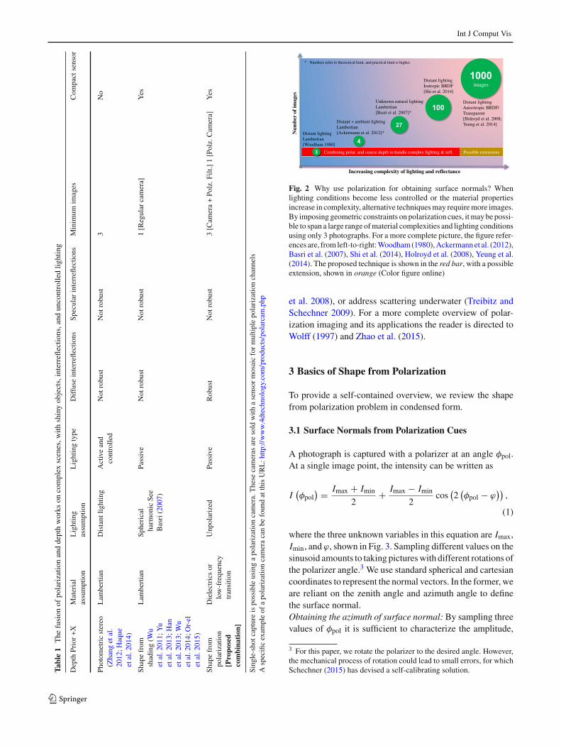
tional measurement of coarse depth to sufficiently addressmajor artifacts in classic SfP, which presents an additionaloption that is complementary to previous works.Combining depth and normal cues is, by now, a popular tech-nique to obtain 3D information. Generally speaking, priorart combines a geometric-based technique to obtain roughdepth with a photometric-based technique to obtain surfacenormals (one of the early works in this line is HelmholtzStereopsis (Zickler et al. 2002)). Such a fusion is well-motivated: (1) The geometric approach helps to remove theambiguities in photometric techniques, such as SfS or uncal-ibrated PS; (2) The photometric approach helps in addingsurface details to the coarse depth map from the geometricdata; and (3) the rough depth map provides anchor points forthe surface-from-gradient problem, addressing the challengeof non-integrable surfaces at depth discontinuities. There arenumerous existing works that partially or completely reflectthese three aspects. Combinations that have been exploredpreviously include: combining a laser scan with PS (Nehabet al. 2005), multi-view stereo with SfS (Wu et al. 2011)or PS (Zhang et al. 2003; Joshi and Kriegman 2007; Este-ban et al. 2008), consumer depth sensing with SfS (Yu et al.2013; Han et al. 2013; Wu et al. 2014), and consumer depthsensing with PS (Zhang et al. 2012; Haque et al. 2014; Shiet al. 2014). If high-quality surface normals are not available,fusing a sequence of overlapping depth maps is a popularapproach to produce a smooth surface for various interac-tive applications (Izadi et al. 2011) or large-scale, real-timesurface reconstruction (Nießner et al. 2013). Table 1 summa-rizes the benefits and limitations of our proposed approach,while Fig. 2 outlines the logic of using polarization insteadof SfS and PS.Polarization in computational imaging: Some researchershave exploited polarized spherical gradient illumination pat-terns coupled with a polarizer in front of a camera to capturethe behavior of polarized light transport for high-resolutionfacial scanning of static expressions (Ma et al. 2007), esti-mation of specular roughness and anisotropy (Ghosh et al.2009), inference of per-pixel surface reflectance parame-ters through circular polarization cues (Ghosh et al. 2010;Guarnera et al. 2012), and for multi-view facial performancecapture (Ghoshet al. 2011). Polarization cues are also widelyused in computational imaging applications, such as sepa-ration of multipath information in ToF imaging (Wallaceet al. 1999), separation of diffuse and specular reflections(Nayar et al. 1997; Zickler et al. 2006), dehazing of images(Schechner et al. 2001), image mosaicing and panoramicstitching (Schechner and Nayar 2005), illumination multi-plexing (Cula et al. 2007), vehicular detection (Dickson et al.2015) and camera (Manakov et al. 2013; Jayasuriya et al.2015) or display hardware (Lanman et al. 2011). In addition,polarization cues can be used to recover shape of translucentobjects (Chen et al. 2007), shape of the ocean surface (Zappa

123

Int J Comput Vis

Tabl

e1

The

fusion

ofpo

larizatio

nanddepthworks

oncomplex

scenes,w

ithshinyob

jects,interrefl

ectio

ns,and

uncontrolle

dlig

hting

Depth

Prior+X

Material

assumption

Lighting

assumption

Lightingtype

Diffuse

interreflectio

nsSp

ecular

interreflectio

nsMinim

umim

ages

Com

pactsensor

Photom

etricstereo

(Zhang

etal.

2012

;Haque

etal.2

014)

Lam

bertian

Distant

lighting

Activeand

controlled

Not

robust

Not

robust

3No

Shapefrom

shading(W

uetal.2

011;

Yu

etal.2

013;

Han

etal.2

013;

Wu

etal.201

4;Or-el

etal.2

015)

Lam

bertian

Spherical

harm

onicSee

Basri(200

7)

Passive

Not

robust

Not

robust

1[R

egular

camera]

Yes

Shapefrom

polarizatio

n[P

ropo

sed

com

bina

tion

]

Dielectrics

orlow-frequ

ency

transitio

n

Unpolarized

Passive

Robust

Not

robust

3[C

amera+Po

lz.F

ilt.]1[Polz.Cam

era]

Yes

Single-shotcapture

ispossibleusingapolarizatio

ncamera.These

cameras

aresold

with

asensor

mosaicformultip

lepolarizatio

nchannels

Aspecificexam

pleof

apo

larizatio

ncameracanbe

foun

datthisURL:h

ttp://www.4dtechnology.com/products/polarcam

.php

Combining polar. and coarse depth to handle complex lighting & refl.

Num

ber

of im

ages

Distant lightingLambertian[Woodham 1980]

3

Increasing complexity of lighting and reflectance

Distant + ambient lightingLambertian[Ackermann et al. 2012]*

Unknown natural lightingLambertian[Basri et al. 2007]*

Distant lightingIsotropic BRDF [Shi et al. 2014]

Distant lightingAnisotropic BRDF/Transparent[Holroyd et al. 2008;Yeung et al. 2014]

* Numbers refer to theoretical limit, and practical limit is higher.

4

27

100

1000images

Possible extensions

Fig. 2 Why use polarization for obtaining surface normals? Whenlighting conditions become less controlled or the material propertiesincrease in complexity, alternative techniquesmay requiremore images.By imposing geometric constraints on polarization cues, itmaybe possi-ble to span a large range ofmaterial complexities and lighting conditionsusing only 3 photographs. For a more complete picture, the figure refer-ences are, from left-to-right:Woodham(1980),Ackermannet al. (2012),Basri et al. (2007), Shi et al. (2014), Holroyd et al. (2008), Yeung et al.(2014). The proposed technique is shown in the red bar, with a possibleextension, shown in orange (Color figure online)

et al. 2008), or address scattering underwater (Treibitz andSchechner 2009). For a more complete overview of polar-ization imaging and its applications the reader is directed toWolff (1997) and Zhao et al. (2015).

3 Basics of Shape from Polarization

To provide a self-contained overview, we review the shapefrom polarization problem in condensed form.

3.1 Surface Normals from Polarization Cues

A photograph is captured with a polarizer at an angle φpol.At a single image point, the intensity can be written as

I(φpol

) = Imax + Imin

2+ Imax − Imin

2cos

(2

(φpol − ϕ

)),

(1)

where the three unknown variables in this equation are Imax,Imin, and ϕ, shown in Fig. 3. Sampling different values on thesinusoid amounts to taking pictureswith different rotations ofthe polarizer angle.3 We use standard spherical and cartesiancoordinates to represent the normal vectors. In the former, weare reliant on the zenith angle and azimuth angle to definethe surface normal.Obtaining the azimuth of surface normal: By sampling threevalues of φpol it is sufficient to characterize the amplitude,

3 For this paper, we rotate the polarizer to the desired angle. However,the mechanical process of rotation could lead to small errors, for whichSchechner (2015) has devised a self-calibrating solution.

123

Int J Comput Vis

phase, and offset of the received signal. The azimuth angle, ϕis encoded as the phase of the received signal. However, notethat the solution is not unique: two azimuth angles, shiftedapart by π radians cannot be distinguished in the polarizedimages.Concretely, note that an azimuth angle ofϕ andϕ+π

return the same value for Eq. 1. In practice, this leads todisappointing results when using shape from polarization.Solving this ambiguity is one focus of this paper.Obtaining the zenith of surface normal: The degree of polar-ization is based on the amplitude and offset of Eq. 1 and canbe written as

ρ = Imax − Imin

Imax + Imin. (2)

Substituting the Fresnel equations (see Hecht (2002)) intoEq. 2 allows the degree of polarization to be written as

ρ =(n − 1

n

)2sin2θ

2 + 2n2 − (n + 1

n

)2sin2θ + 4 cos θ

√n2 − sin2θ

, (3)

where n denotes the refractive index and θ the zenith angle.If the refractive index is known, the zenith angle can be esti-mated either in closed-form, or by numerical optimization.Unfortunately, it is difficult to know the refractive index ateach pixel, particularly in a scene with mixed materials; thisis one of the challenges with SfP that we address.Specular vs diffuse polarization: Equation 3 is robust fordielectric surfaces, but cannot be used on non-dielectric sur-faces, such asmirrors ormetals. Thesematerials do not reflectback any diffuse light, but the relation

ρ = 2n tan θ sin θ

tan2 θ sin2 θ + |n∗|2 , (Specular Model) (4)

where |n∗|2 = n2(1 + κ2

)and κ is the attenuation index of

the material, allows the zenith angle to be found (Morel et al.2005). It is possible to identify whether to use Eqs. 3 or 4 toobtain the zenith angle based on the degree of polarizationat a single pixel.4 Variants of the method thus described areimplemented in previous SfP work (Atkinson and Hancock2005; Miyazaki et al. 2004, 2003). Due to the limitationsof SfP (see bullets 1–3 from Sect. 1), SfP has never beenconsidered as a robust alternative to SfS or PS.Implementing shape from polarization: Although SfP hasmany ambiguities, as described above, our method uses stan-dard SfP to recover an initial normal map from polarization.This will have all the aforementioned ambiguities, but ourcontribution is to correct it with geometric constraints. Toobtain the initial normal map, we choose a refractive index

4 In practice, the degree of polarization is generally an order of magni-tude larger for specular dominant reflections.

to 1.5 (this value is obviously wrong, but is close to the real-world value of many common objects). To decide whetherEqs. 3 or 4 is more germane, we make the observation that ifρ is high, the reflection is specular, and the latter equation ismore relevant. The result from SfP on the coffee cup sceneis shown in Fig. 1c, where the challenges with SfP can bereadily observed.

4 Framework for Depth-Polarization Fusion

Scenes are assumed to have the following properties: (1)unpolarized ambient light; (2) no specular interreflections;(3) only dielectric materials or low-frequency changes inmaterials; and (4) diffuse-dominant or specular-dominantsurfaces.5

4.1 Correcting Normals from Polarization

We use the obtained depth map to correct systematic dis-tortions in the normals from polarization. Let D ∈ R

M×N

denote the obtained depth map. Our correction scheme oper-ates in the normal domain, so we find the surface normalsfrom the depth map, denoted as Ndepth ∈ R

M×N×3. Fol-lowing the work of Klasing et al. (2011), we express thedepth map D ∈ R

M×N as a point cloud of real-world coor-

dinates as Px,y =[− u

fxDx,y − v

fxDx,y Dx,y

]T, where u

and v denote pixel coordinates and fx and fy denote thefocal length in units of pixels. For each scene point Px,y , wefind J points whose Euclidean distance away from Px,y isless than a fixed absolute distance.6 Thus, for a given point,Px,y , we have a set that includes this point and its neighbors,{Px,y, Px1,y1 , . . . , PxJ ,yJ

}. By stacking all of these points

into a matrix,

Q =

⎡

⎢⎢⎢⎣

−− PTx,y −−

−− PTx1,y1 −−...

−− PTxJ ,yJ −−

⎤

⎥⎥⎥⎦

, (5)

we find the normal by solving

Ndepthx,y = argmin

n

∥∥(Q − Q

)n∥∥22 ,

where each identical row of the matrix Q ∈ R(J+1)×3 con-

tains the mean across the first dimension of Q (i.e., a pointthat is the average of all the points in Q). The smoothness of

5 Refer to Sect. 5 for a detailed analysis of key assumptions.6 For all experiments, this distance was set to 20 millimeters. To findthe neighborhood, we use the kd-tree search algorithm, which can beimplemented by the rangesearch command in MATLAB.

123

Int J Comput Vis

(a) (b)

(d)

(c)

Fig. 3 Capture setup. In a a standard camera with a polarizing filteris used to photograph a diffuse sphere under different filter rotations.The Kinect is not used in this figure, but shown for context (as the restof the paper uses the Kinect). b A photograph of the sphere with twopoints on the geometry labeled. c Plotting intensity at different polar-izer angles at the labelled points on the geometry. Observe the variation

in the sinusoid that is due to the geometry. d Selected photos of theobject at different polarizer angles show a slight variation (figure mustbe viewed digitally). a Capture setup; b photograph of object; c inten-sity versus polarizer angle; d photographs at different polarizer anglesshow slight variation

Ndepth can be changed by controlling the size of the neigh-borhood that the search algorithm returns.

4.1.1 Removing Low-Frequency Azimuthal Ambiguity

Consider the corner scene in Fig. 4. Using a coarse depthsensor, a low-frequency version of the surface is acquired(note the smoothness in the 3D shape in Fig. 4b). On the otherhand, the shape from polarized normals is very inaccuratedue to the azimuthal flip, but the high-frequency detail canbe recovered.

Let Npolar ∈ RM×N×3 denote the normal map obtained

frompolarization cues.7 The goal is to find an operatorA thatrelatesNpolar andNdepth, which can be expressed numericallyas

A = argminA

∥∥∥Ndepth − A(

Npolar)∥∥∥

2

2.

Without any additional constraints, this optimization is ill-posed. However, to resolve polarization ambiguity we are

7 Npolar is obtained through shape from polarization and this normalmap will suffer from the physics-based artifacts described previously.This can be seen visually in Fig. 1c.

only interested in representing A as a binary operator, i.e.,the operator A has a matrix representation A of dimensionM × N , where A ∈ 0, 1. Here, the binary state of each ele-ment, Amn , corresponds to whether a normal at a specificpixel location will undergo an azimuthal rotation or not. Theoperator’s function follows suit: at each pixel, the operatorA either rotates the azimuth angle by π or does nothingdepending on the binary value of Amn . Since the goal is tosolve low-frequency ambiguity,we impose an additional con-straint that the matrix representation of A is smooth in thesense of total variation. Taken together, this can be expressedas a minimization problem:

A = argminA

∥∥∥Ndepth − A(

Npolar)∥∥∥

2

2+ γT2 (A)

subject to A ∈ {0, 1

}, (6)

where the parameter γ controls the (piecewise) smoothnessof the solution andT2 is the standard 2DTV regularizer, suchthat T2 (A) = ∑

m∑

i |∇xAmn| + |∇yAmn|, where ∇x and∇y are horizontal and vertical gradients. In particular, sincethe decision variable is binary, we use a modified version

123

Int J Comput Vis

(a) (b) (c) (d)

(e) (f) (g) (h)

(i) (j) (k)

(l) (m) (n)

Fig. 4 A commonly used benchmark scene (Gupta et al. 2015; Naiket al. 2015). Combining polarization with Kinect results in improvedperformance. The top row shows the 3D shape of a corner. The secondrow shows the surface normals. The third row plots the estimated surfaceerror in millimeters and the fourth row depicts the estimated angularerror of surface normals in degrees w.r.t. the ground truth. a 3D Shapeground truth; b 3D shape kinect; c 3D shape polarization; d 3D shapeour result; e surface normals groundtruth; f surface normals kinect; gsurface normals polarization; h surface normals our result; i shape errorkinect (5.4 mm); j shape error polarization (37.6 mm); k shape errorour result (3.6 mm); l normal error kinect (20.9 deg); m normal errorpolarization (68.5 deg); n normal error our result (4.6 deg)

of graph-cuts, which is often used to segment an image intoforeground and background patches. 8 After obtaining A itis possible to correct low-frequency changes in the ambiguityby applying the operator to the polarization normal:

Ncorr = A(

Npolar)

. (7)

After correcting for low-frequency ambiguity, we can returnto the physical experiment on the corner. By applying thetechniques introduced in this section we have traversed fromthe ambiguous normals in Fig. 4g to the correctly flippednormals in Fig. 4h. For this example, the ambiguity was low-frequency in nature, so the coarse depth map was sufficient.

8 The 2D-TV implementation parallels the optimization program fromprior work (Kadambi and Boufounos 2015).

(a) (b)

(c)

Fig. 5 Addressing high-frequency ambiguity. Consider a planar sur-face with a high-frequency pit. a Anchor and pivot points are identifiedto group points on the ambiguity region into (b) facets. c Each facet canbe rotated by π radians, creating ambiguities. a Point identification; bfacets; c six possible orientations

4.1.2 Removing High-Frequency Azimuthal Ambiguity

If the depth map is coarse, consisting of low-frequencyinformation, then it cannot be used to resolve regions withhigh-frequency ambiguity. To address this challengewe forcethese regions of the surface to be closed.

Figure 5a illustrates a conceptual example with a high-frequency V-groove on a plane. The normals are disam-biguated correctly on the plane, but the ridge cannot bedisambiguated using the method from Sect. 4.1.1. In par-ticular, observe that the high-frequency ridge can take oneof six forms. To constrain the problem, we define an anchorpoint at the start of the high frequency region and a pivotpoint at the center of the ridge. The anchor point representsthe boundary condition for the high-frequency ridge and thepivot point occurs on an edge not on the boundary.

Given the anchor and pivot points, we define a facet as theset of points between the anchor andpivot points (seeFig. 5b).A facet can form a planar or nonplanar surface. Assumingthere are K facets, there are 2 × 2K − V possible surfaceconfigurations, where V is the number of possible closedsurfaces.9 This surface has two facets and two closed config-urations, and therefore six possible surface configurations.Four of these are not closed, i.e., the high-frequency regionhas a discontinuity at an anchor point. The discontinuity isphysically possible—i.e., the V-groove could actually be aramp in the real world—but it is less likely that the high fre-quency detail has such a discontinuity exactly at the anchor

9 Calculation of 2 × 2K − V : each facet can have 2 possible normalorientations due to the azimuthal ambiguity, leading to 2K possible sur-face configurations due only to the degrees of freedom of the facets. Byconstraining the rest of the surface using the anchor point as a bound-ary condition, this leads to 2 × 2K surface configurations. Since weassume that the facet is continuous with the anchor point, the overalldimensionality is reduced to 2 × 2K − V .

123

Int J Comput Vis

(a) (b) (c) (d)

Fig. 6 Within the dielectric range (n=1.3 to 1.8), refractive distortionhas little effect on shape reconstruction (simulated example). We simu-late a scenewith three spheres, each having different material propertiesbut geometrically identical. If the refractive index is unknown—and ahard-coded threshold is used—the estimated surface normals shown

in the bottom row of a–c exhibit slight distortion. When the surfacesare integrated, shown in the upper row of (a)–(c), the shape changesslightly, shown in d a Refract. index=1.3; b Refract. index=1.5; cRefract. index=1.8; d recovered surface

point. Therefore, we assume the high-frequency surface isclosed.10 Of the two closed surfaces, one is concave and theother is convex. There is no way to distinguish between thesesurfaces using polarization cues. This is not unique to polar-ization enhancement: the convex/concave ambiguity appliesto the entire surface from SfS (Oliensis 1991) and uncali-brated PS (Yuille and Snow 1997).

4.1.3 Correcting for Refractive Distortion

Recall that estimation of the zenith angle requires knowledgeof the refractive index. For materials within the dielectricrange, deviation in the estimated zenith angle is only a minorsource of error (Fig. 6). However, for non-dielectrics, thezenith angle surface normal will be distorted, which whenintegrated, causes distortions to the 3D shape.

To undistort the zenith angle, we first find the regions ofthe depth map that provide a good estimate of the coarseobject shape. Specifically, we define a binary mask as

Mx,y = 1 if |∇T Ndepthx,y | ≤ ε and |∇T Ncorr

x,y | ≤ ε,

Mx,y = 0 o.w., (8)

10 Implementing high-frequency ambiguity correction. First, a differ-ence image is formed of the depth normals and polarization normals.The difference image only contains detailed features, as it would notshow up in the former (otherwise the method from Sect. 4.1.1 wouldhave been sufficient). From the difference image, the pixel at an edgefrom 0 to a non-zero value represents an anchor point. An edge corre-sponding to a change in sign (e.g., at the V-groove of a corner) is a pivotpoint. A greedy approach is used to flip surface facets, which enforcesa closed surface constraint. Details about the closed surface constraintcan be found in Miyazaki et al. (2003).

where ε is a smoothness threshold. Note that the depth maphas been smoothed, such that it is not noisy, but lacks finedetail. Intuitively, Eq. 8 is saying that if the depth map haslow divergence (the depth map predicts no detail) and thepolarization data has low divergence (it is either noisy or pre-dicts no detail), then we should use the depth normal. For thecorner in Fig. 4, observe that the sharp point of the corner—where the Kinect data is inaccurate due to multipath—has amask value of 0 since the divergence in Ncorr is high.

Let θdepth ∈ RM×N and θcorr ∈ R

M×N denote the zenithcomponents of Ndepth and Ncorr from Sect. 4.1.1. Over thepixel grid, we use a patch based optimization. A patch isa rectangular group of P pixel coordinates with associated,

scalar angles from depth,{θdepthx1,y1 , . . . , θ

depthxP ,yP

}and polariza-

tion,{θcorrx1,y1 , . . . , θ

corrxP ,yP

}.11 For the p-th patch, the goal is

to find a rotation operator Rp, such that

Rp = argminR

P∑

i=1

Mxi ,yi |θdepthxi ,yi − R(θcorrxi ,yi

)|2. (9)

To correct for refractive index, the normals are updatedby applying the rotation operator to pixels within this patch,such that

Ncorrxi ,yi := sph2cart

(1,Rp

(θcorrxi ,yi

), ϕxi ,yi

), (10)

where ϕxi ,yi denotes the azimuth angle of Ncorrxi ,yi , sph2cart

represents an operator that converts spherical coordinates tocartesian, and the first argument of sph2cart is the radial

11 Note: this notion of a patch operates on the pixel grid and is thusdifferent from our convention of defining a point cloud neighborhood(cf. Sect. 4.1). For our paper, we use a 7x7 patch.

123

Int J Comput Vis

distance, typically equal to 1 for surface normals. It is impor-tant to note that Rp is applied on a patch-wise basis as it willbe different at different patches (due to the spatially-varyingnature of the problem).

4.2 Corrected Normals from Polarization to Enhancethe Coarse Depth Map

Given the corrected normals, it is possible to integrate toobtain the 3D shape. Unfortunately, surface normal inte-gration is known to be a challenging task due to depthdiscontinuities (Agrawal et al. 2006; Zhang et al. 2012).To recover plausible 3D shape, we develop an integrationscheme that incorporates the input depth map (D) and phys-ical intuition from corrected polarization normals (Ncorr) torecover the depth coordinates of the surface D ∈ R

M×N .

4.2.1 Spanning Tree Constraint

The standard way to integrate surface normals uses the well-known Poisson equation, written as ∇2D = ∇T Ncorr forour problem. This is the optimal solution in the sense of leastsquares and works well when the noise model is asystematic.

For the polarization problem, the surface normals havesystematic error. Intuitively, it is desirable to avoid inte-gration using unreliable surface normals (see Fig. 7). Inparticular, the surface can be recovered in closed form byusing only the minimum spanning tree over a weighted, 2Dgraph (the spanning tree is found using Kruskal’s algorithm).The optimal solution is written as

∇2SD = ∇T

S Ncorr, (11)

where S denotes the set of gradients used in the reconstructionand ∇2

S and ∇TS represent Laplace and divergence operators

computed over S. For accurate integration, the set S includesa spanning tree of the graph. Let Wx,y denote the weightsof the 2D grid. To find the weights, most previous work useseither random sampling, gradient magnitudes, or constraintson integrability (Agrawal et al. 2006; Fraile and Hancock2006).

The physics of polarization are used to motivate the selec-tion of graph weights. Specifically, the polarization normalsare considered to be noisy when the degree of polarization ρ

is low.12 A lowdegree of polarizationmost commonly occurswhen the zenith angle is close to zero (i.e. fronto-parallel sur-faces). For the depth map, the mask operator M, defined inSect. 4.1.3, provides a weight of confidence.

We initialize S, the set of gradients used in the integration,as the empty set. The first gradients that are added to S are

12 Estimation of the sinusoidal parameters fromEq. 1 becomes unstablewhen there is little contrast between Imin and Imax.

Fig. 7 Using polarization cues to find the best gradients to integrate thesurface (simulated example). Represent the image points as nodes andgradients as edges. The full gradients are shown in the upper-left. Webreak the edges that have a low degree of polarization to find aminimumspanning tree for the grid (upper right). We validate this in simulation,shown at bottom, where the normals from polarization have error infronto-parallel regions. Full integration results in a noisy depth map,while the spanning tree integration preserves the shape of the contour

those that lie on the minimum spanning tree of the weightedgraph with weights

Wx,y = ρx,y if ρx,y > τ and Mx,y = 0,

Wx,y = τ otherwise, (12)

where τ reflects the level of confidence in the polarizationvs depth normals. We then update S by using the iterative α-approach described in Agrawal et al. (2006) by using Ncorr inthe update process. To incorporate Ndepth into the approach,we update the corrected normals using the output from theα-approach, i.e.,

Ncorrx,y := Ndepth

x,y if Wx,y ≤ τ. (13)

4.2.2 Depth Fidelity Constraint

When integrating surface normals, only a relative 3D shapeup to an unknown offset and scaling is obtained. Here, thedepth fidelity constraint serves to preserve the global coordi-nate system and enforce consistency between the integratedsurface and accurate regions of the depth map. Specifically,the depth constraint takes the form of

∥∥vec(M � (

D − D))∥∥2

2 , (14)

123

Int J Comput Vis

where vec denotes the vectorization operator and � repre-sents Hadamard multiplication. Here, we have usedHadamard multiplication with the mask to enforce fidelityonly where the depth map is reliable. Both the depth fidelityand spanning tree constraints are incorporated into a sparselinear system

[λM � I

∇2S

]vec

(D

) =[

λvec (M � D)

∇TS (Ncorr)

], (15)

where I is the identity matrix of size MN × MN and λ is ascalar parameter to adjust the tradeoff between spanning treeand depth fidelity constraints.13

5 Reflection and Lighting Assumptions

This section analytically validates the practicality of our tech-nique by justifying the reflectance and lighting assumptions,first described in Sect. 4. Specifically, Sect. 5.1 includes twopropositions, one for the azimuth angle, the other for thezenith angle, to explain why the proposed method will workon certain classes of mixed surfaces but not others (e.g., if areflection is 75 percent specular and 25 percent specular, themethod can work, but not if the components are equal). InSect. 5.2 the unpolarized world assumption is described inmore detail.

5.1 Analyzing Mixed Reflections

Reflections from real-world objects aremixed as they includeboth specular and diffuse components.14 In this paper, we areable to recover 3D geometry for mixed surfaces, subject tothe constraint that the reflection is composed of an unequalmixture of diffuse and specular components. We term thisthe “diffuse or specular dominant” assumption, first listed inSect. 4.

One of the reasons for this assumption is that when themeasured irradiance from diffuse and specular reflectioncomponents is small wrt. noise, then the azimuthal angleencounters a stochastic additional ambiguity of π/2 radians.We refer to this error as stochastic azimuthal ambiguity. Incomparison, when the measured irradiance from the reflec-tion components is large wrt. noise, then the azimuthal anglepredictably aligns to either diffuse or specular reflection com-ponents.

13 A value of λ = 0.02 is recommended.14 In this paper, we use the term “reflection components” following anoptical imaging convention. This is identical to the term “reflectancecomponents”, which may be more familiar to some readers.

Proposition 1 Stochastic ambiguities in the azimuthal angleare avoided when polarized reflections are either diffuse orspecular dominant.

Proof Consider a single scene point where the image inten-sity of a mixed reflection can be written as

I = IS + ID, (16)

where IS is the intensity due to a specular reflection, whileID is due to a diffuse reflection. Both specular and diffusereflections will have polarized (denoted by IS) and unpo-larized components (denoted by IS). Then, IS = IS + ISand ID = ID + ID . The total image intensity can now beexpressed as

I = IS + IS + ID + ID . (17)

Writing this in terms of electric field vectors,

E = E0 + ED + ES, (18)

where the unpolarized electric field vector E0 can have anydirection. By noting that the diffuse and specular componentsdiffer in phase by a factor of π/2, we write

E = E0 + ED sin(φpol − ϕ

) + ES cos(φpol − ϕ

), (19)

where φpol is the polarizer angle, and ϕ the azimuth angle atthis scene point. Since the light source is incoherent, upontaking the magnitude, we obtain

I = |E| = I0 + ID sin2(φpol − ϕ

) + IS cos2 (

φpol − ϕ),

(20)

which is rearranged as

I = I0 + IS + ID2

+ IS − ID2

cos(2

(φpol − ϕ

)). (21)

Clearly if the surface is specular dominant, then IS � IDand Eq. 21 can be approximated as

I = I0 + IS2

+ IS2cos

(2

(φpol − ϕ

)). (22)

Similarly, if the surface is diffuse dominant, then IS � IDand Eq. 21 can be approximated by neglecting IS . Note thateither IS ≥ ID or IS < ID . Represent = |IS − ID|.Then, depending onwhether the diffuse or specular polarizedcomponent is greater, Eq. 21 can be written as

123

Int J Comput Vis

I = I0 + IS + ID2

+

2cos

(2

(φpol − ϕ

))if IS ≥ ID

I = I0+ IS+ ID2

+

2cos

(2

(φpol−(ϕ−π/2)

))if IS < ID,

(23)

where now the azimuth angle has shifted by π/2 radians.Only for small values of will the flip in azimuthal anglebe randomly dependent on noise. Specifically, if is large,the model will consistently conform to one of the two casesin Eq. 23, which is the desired result. �

The key implication of Proposition 1 is that azimuthalangle is robust to mixed surfaces as long as the assumptionof diffuse/specular dominance is met and that the correctmodel, either diffuse/specular, is identified.

We now seek to show that any perturbation in zenith angleas a function of mixed reflectance can be corrected for withdepth constraints.

Proposition 2 Assuming the conditions of Proposition 1hold, perturbations in zenith angle due to mixed reflectionscan be corrected by applying the rotation operator R, asdescribed in Eq. 10.

Proof Under the conditions of Proposition 1, it is assumedthat the reflection component is either (1) specular dominant,or (2) diffuse dominant. First, consider case (1). Denote Imin,Imin, and ρ as the corresponding variables of Imin, Imin, and ρ

for mixed reflections. Since, for case (1), I = IS + ID ≈ IS ,it follows from Eqs. 1 and 21 that:

Imin = ID,

Imax = IS,

ρ = IS − ID2I0 + IS + ID

= IS − ID2(IS + ID) + IS + ID

.

(24)

Now, ρ is dependent on both diffuse and specular compo-nents. Under case (1), the polarization of diffuse componentis assumed to be negligible wrt. the polarization of the spec-ular component. Therefore, the relation in Eq. 16 allows usto express the measured degree of polarization, after simpli-fication, as:

ρ = ρI − ID

I. (25)

Since I−IDI acts as a scaling factor on the degree of polar-

ization, and since the degree of polarization has a monotonicrelationship with zenith angle, it follows that ∃ a rotationoperator that aligns the mixed zenith angle with the truezenith angle. For case (2), the opposite is assumed, such thatthe measured degree of polarization is expressed as:

ρ = ρI − IS

I. (26)

(a)

(b)

(c)

(d)

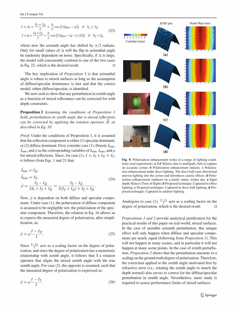
Fig. 8 Polarization enhancement works in a range of lighting condi-tions (real experiment). a ToF Kinect, due to multipath, fails to capturean accurate corner. b Polarization enhancement indoors. c Polariza-tion enhancement under disco lighting. The disco ball casts directionaluneven lighting into the corner and introduces caustic effects. d Polar-ization enhancement outdoors on a partly sunny, winter day. a Inputdepth: Kinect (Time of flight); b Proposed technique: Captured in officelighting; c Proposed technique: Captured in disco ball lighting; d Pro-posed technique: Captured in outdoor lighting

Analogous to case (1), I−ISI acts as a scaling factor on the

degree of polarization, which is the desired result. �

Propositions 1 and 2 provide analytical justification for thepractical results of this paper on real-world, mixed surfaces.In the case of unstable azimuth perturbation, this uniqueeffect will only happen when diffuse and specular compo-nents are nearly equal (following from Proposition 1). Thiswill not happen in many scenes, and in particular it will nothappen at many scene points. In the case of zenith perturba-tion, Proposition 2 shows that the perturbation amounts to ascaling on the ground truth degree of polarization. Therefore,the correction applied to the zenith angle motivated first byrefractive error (i.e., rotating the zenith angle to match thedepth normal) also serves to correct for the diffuse/specularperturbation in zenith angle. Nevertheless, more study isrequired to assess performance limits of mixed surfaces.

123

Int J Comput Vis

5.2 Unpolarized World Assumption

This paper follows the standard SfP assumption that the lightincident on the object is unpolarized, such that any polariza-tion imparted to the reflected light is due to the shape. For thisto hold, the light source must be unpolarized and the scenemust not consist of specular interreflections.Incident lighting is unpolarized: Natural light sources, likethe sun, are unpolarized. Most types of indoor lighting arealso unpolarized, like incandescent or halogen bulbs. Some-times, solid-state light sources are used indoors, like LEDlamps. However, in almost all cases, a diffusing sheet isplaced over the light source, which acts to depolarize thelight. We believe that the unpolarized source assumption isvalid.No specular interreflections assumption Assuming the lightsource is unpolarized, after a specular reflection, the light ispolarized. If this is incident on the scene point of interest,the polarimetric properties of the reflected light will not bedue solely to the shape. In practice, the presence of specularinterreflections is a limiting factor for most of the popularshape depth sensing technologies (e.g., structured light, timeof flight, photometric stero, shape-from-shading). We feelthat this is likely the most serious limitation for SfP and, byextension, our proposed technique. For example, even thoughthe sun is unpolarized, due to air scattering, the polarizationincident on the surface-level will vary based on factors likethe weather and time of day. An open problem will be how to

make polarization based techniques more viable in outdoorenvironments.

6 Assessment and Results

Previous techniques in shading enhancement have had lim-ited success under challenging material or lighting condi-tions. The proposed technique, using polarization, is able tohandle more complicated scenes.

6.1 Robustness in the Wild

Robustness to lighting conditions: Assuming unpolarizedincident light, the proposed technique is robust to varyinglighting conditions. As shown in Fig. 8, depth enhancementis shown to be near-identical for three lighting conditions:(Fig. 8b) indoor lighting; (Fig. 8c) under interfering illumi-nation from a disco ball; and (Fig. 8d) even outdoors. Thelast two conditions violate lighting assumptions of SfS.Robustness tomaterial properties:Asshown inFig. 9 the pro-posed technique is evaluated on three materials: (1) diffuse;(2) glossy; and (3) mirror-like. Polarization enhancementis consistent for each material, though slightly worse forthe mirror-like object. Comparison papers that use shadingenhancement can onlywork onLambertian surfaces (Yu et al.2013; Han et al. 2013; Wu et al. 2014; Or-el et al. 2015).

(a) (b) (c) (d)

Fig. 9 Polarization enhancement works for variedmaterial conditions.Since one of the objects is shiny, a simulated depth skeleton with addi-tive Gaussian noise is used as the depth template; this demonstrates thatour key contribution of combining a general depth map with polariza-

tion normals can work for a range of material conditions. A challengingobject can preclude recovery of a coarse depthmap, leading to instanceslike the failure case in Fig. 14. a Scene; b three polarization photos; cdepth skeleton; d pol. enhanced

123

Int J Comput Vis

(a) (b)

Fig. 10 The proposed technique can correct multipath interferencein ToF sensors. Comparing the proposed technique against Naik etal. (2015), which combines ToF with structured illumination patternsfrom a projector. The technique by Naik et al. uses 25 coded illumina-

tion photographs. With 3 photographs from a polarizer and the Kinectdepth map, the proposed technique preserves the sharp edge of groundtruth. a Comparison: Kinect multipath correction (Naik et al. 2015); bThis paper: Fig. 4 Xsection

Robustness to diffuse multipath: Diffuse multipath has beenan active challenge in the ToF community (O’Toole et al.2014; Gupta et al. 2015; Naik et al. 2015). The proposedtechnique of polarization enhancement drastically outper-forms a state-of-the-art technique for multipath correction,while using fewer images (Naik et al. 2015). Refer to thecaption of Fig. 10 for details.

6.2 Results on Various Scenes

Figure 11 shows results on various scenes along with qualita-tive comparisons to shading refinement, directly performedby Wu et al. (2014).Diffuse face scene: Themannequin scene, shown in Fig. 11a,was selected to compare the best-case performance of shad-ing enhancementwith our proposed technique of polarizationenhancement. Specifically, the mannequin is coated withdiffuse paint and lit by distant lighting to conform to SfSassumptions. Even under ideal conditions for shading refine-ment, the proposed technique using polarization leads toslightly improved 3D reconstruction. As shown in the close-up, the concave eye socket causes challenges for shadingrefinement due to diffuse interreflections.Coffee cup scene: Figure 11b shows depth reconstructionfor a coffee cup made of Styrofoam. Such a surface isnot Lambertian, and causes artifacts in shading refinement.The proposed technique is dramatically better than shadingrefinement, and as shown in Fig. 12, is able to cleanly recoverthe grooves (300micron feature size). For this scene, the pro-posed technique outperforms a laser scan of the object (referto Fig. 12 for the comparison).Two-face scene: To illustrate robustness to mixed-materials,Fig. 11c shows a mannequin, painted with two paints ofdifferent pigments and specularities. Shading enhancementcannot handle the shininess of the face, so the entire recon-struction is poor.Moreover, at the point ofmaterial transition,local artifacts are visible (best seen in the close-up). In com-

parison, the proposed technique of polarization enhancementrecovers the surface well, and is robust to material change(see close-up). Note that the lack of artifacts at the pointof material transition verifies that assumption 4 need not bestrict (since the paints have different proportions of diffuseand specular reflectivity).Trash can scene: Figure 11d depicts a scene for every-day objects under natural lighting. The scene consists ofa hard, plastic trash can with a shiny, plastic liner in awell-illuminated machine shop with windows. This is a chal-lenging scene for depth enhancement, with uncontrolledlighting, mixed materials and specular objects. The pro-posed technique performs drastically better than shadingrefinement. In particular, the reconstruction from shadingrefinement contains holes in the recovered surface that cor-respond to specular highlights in the image. Furthermore,since the liner is highly specular, shading refinement cannotresolve the ridges. In comparison, the proposed techniquereconstructs many of the ridges in the liner.Enhancing a laser scanner:Figure 13 shows that polarizationenhancement can be a beneficial additional to even higher-quality depth sensors. As shown in Fig. 13c, given a laserscan of the cup, we corrupt it with quantization and additivenoise to form the depth skeleton. All details are lost in thisskeleton, but after polarization enhancement, details down tothe 300 micron grooves are made visible. Adding a polarizerto a mid-range laser scanner, might be a low-cost solutionto computationally replicate the performance of a higher-quality laser scanner.Failure case: Failure cases occur in the context of all limita-tions detailed in the paper. We illustrate one such failure casein Fig. 14. The depth map obtained from the chrome spherecontains significant error in low-frequency content. Our“enhanced” shape tries to preserve low-frequency fidelitywith the noisy depth map instead of recovering the correctshape.

123

Int J Comput Vis

(a) (b) (c) (d)

Fig. 11 Various captures, ranging from controlled scenes to complex scenes. Please zoom in using your PDF viewer. a Diffuse face scene; b coffeecup scene; c two-face scene; d trash can scene

Fig. 12 Qualitative comparison to a multistripe laser scanner. a Ourresult, using a Kinect and three polarized photographs. b The surfacefrom the laser scanner. Notice that the Kinect has been enhanced to thepoint of capturing the grooves in the cup, approximately 300 micronsin depth. a Enhanced kinect depth; b laser scanner depth

6.3 Quantitative Analysis of Enhancement

Table 2 shows the mean absolute error wrt. a laser scan fora sampling of scenes from this paper. Since shading-basedtechniques (Wu et al. 2014) cannot handle shiny objects likethe chrome sphere or glossy coffee cup, the error actually

increases wrt. the input depth. In contrast, the proposed tech-nique of polarization reduces error for all scenes. Becausepolarization can handle interreflections (which the Kinectcannot), polarization shows the most improvement on thecorner scene. Refer to Fig. 4 for additional metrics.

To verify the resolution enhancement of the proposedapproach, we used a precision caliper to measure the groovesof the cup in Fig. 11c at 300microns. The proposed techniquecan resolve finer detail than some laser scanners.

6.4 Implementation Details

As shown in Fig. 3, the capture setup includes the following:a Canon Rebel T3i DSLR camera with standard Canon EF-S18-55mm f/3.5-5.6 IS II SLR lens, a linear polarizer withquarter-wave plate, model Hoya CIR-PL. Calibration is per-formed on the polarizer’s transmission axis. Values for τ andε are the same for all scenes. The latest model of MicrosoftKinect is used to obtain most depth maps. Normal maps anddepthmaps are registered using the intrinsic parameters of theKinect and relative pose (translation only). Tomeasure polar-ization cues the sensor response must be linear, enforced bypreprocessing CR2 raw files from the camera. Ground truth

123

Int J Comput Vis

(a) (b) (c)

Fig. 13 Our technique can be used to augment even high quality depthmaps (physical experiment). a The Styrofoam cup being laser scannedusing multistripe technology. b We can combine the direct output fromthe laser scan with polarization cues to recover even more detail. c Thelaser scanner output is corrupted with additive Gaussian and quantiza-

tion noise. Polarization cues are still able to recover the ridges on thecup. The ridges are approximately 300 microns in depth. This figure isbest viewed digitally. a Setup; b enhancing the laser scan; c corrupteddepth skeleton

Fig. 14 A failure case due to lack of low-frequency shape informationin the depth skeleton (physical experiment). a The scene is a chromesphere. b The Kinect depth has an incorrect shape due to the specu-larities. c Our polarization enhanced algorithm takes the characteristicsof the distorted depth skeleton. a Chrome sphere; b kinect depth; cpolarization enhanced

Table 2 Mean absolute error (mm) with respect to a laser scanner

Init. depth Shading (Wu et al. 2014) Proposed

Corner, Fig. 4 5.39 4.78 3.63

Mirror ball, Fig. 9 8.50 17.58 8.25

Diffuse face, Fig. 11a 18.58 18.30 18.28

Coffee cup, Fig. 11b 3.79 3.84 3.48

is obtained using a multi-stripe, triangulation, laser scannerand benchmarks are obtained through ICP alignment.15

7 Discussion

In summary, we have proposed the first technique of depthenhancement using polarization normals. Although shading

15 Laser Scanner: http://nextengine.com/assets/pdf/scanner-techspecs.pdf.

refinement is an established area, with incremental progresseach year, the proposed technique leverages different physicsto demonstrate complementary advantages.Benefits: By using the depth map to place numerous con-straints on the shape-from-polarization problem, this paperresolves many of the ambiguities in shape-from-polarizationresearch while demonstrating compelling advantages overalternative techniques (SfS and PS). In particular, SfS and PSassume Lambertian objects and distant/controlled lighting,while the proposed technique has demonstrated results ondiffuse to mirror-like objects in controlled and uncontrolledsettings.16 Moreover, the proposed technique can be madepassive, can be implemented in a single-shot, and requiresno baseline (Table 1). While not specific to multipath cor-rection, the proposed technique, while using fewer images,can outperform a paper entirely dedicated to ToF multipathcorrection (Fig. 10).Material assumptions Although we have presented practicalresults on a range of materials, the technique is still sensitiveto certain material configurations. For example, if the mate-rial change is rapid in a scene (like glitter on an object), theproposedmethodwould fail (as it relies on patches with fixedmaterial properties). An engineering improvement would beto use higher spatial resolution sensors, as sensors continue toincrease in resolution. On amore fundamental level, inspiredby the work of Huynh et al. (2013), it may be possible touse additional information from different spectral channels

16 While there are variants of generalized photometric stereo for non-Lambertian objects and natural environment lighting, they usuallyrequire about 50-100 images according to a recent survey in Shi et al.(2016).

123

Int J Comput Vis

to recover the refractive index. Another area of future workwould be to explore how layered or transparent materialswould affect the polarimetric approach. A clear advantage ofapproaches that rely on polarization is that they generalize tonon-Lambertian surfaces, like metals. For the proposed workto generalize to metallic surfaces, the key challenge lies inobtaining the depth of a metallic object.Shape from mixed polarization: As of today, the communityhas developed models for diffuse or specular polarization(Equations. 3 and 4, respectively). But a ‘mixed reflection’will consist of light that is both diffusely and specularlyreflected. This causes model mismatch (as the model doesnot conform to either Eqs. 3 and 4). Mixed reflections havebeen a problem for prior work that uses only polarimetricinformation. However, in this paper, we have shown thatthe depth constraints we impose offer a degree of robust-ness to mixed reflections. This has been shown analyticallyin Sect. 5.1 of this paper and verified with practical results.We must emphasize that our solution is not perfect—we stillrequire diffuse-dominant or specular-dominant surfaces (sothat we can pick whether to use Eqs. 3 and 4 for the initialnormal map from polarization).Practical applications: The proposed work offers com-plementary benefits to shading or photometric solutions,offering 3D scans of objects that may be shiny or lit byarea sources. Although we used a capture setup that wasnot real-time (since we took three photos at three differentpolarizer rotations), there are off-the-shelf camera systemsthat allow single-shot capture. With a production budget, wehave little doubt that the implementation could be a 2-frame,real-time technique (the 2 frames would be a depth frame,and the single-shot frame from the polarization array cam-era).However, themethodhas value even as a static technique(as demonstrated in this research paper) where the obtainedresults can be seen as compelling; for example, in Fig. 12,the proposed technique outperforms a scan of the coffee cupscene captured with a multi-thousand dollar professional-grade 3D scanner (that is also not real-time). Moreover, theproposed technique (depth and polarization) is a new direc-tion to probe, which could be combined with other sourcesof information.Limitations: The proposed technique requires 3 images forcapturing the polarimetric information; however, off-the-shelf solutions allow single-shot polarimetric capture.17 Forrobust performance, the assumptions described in Sect. 4and Table 1 must be met. Note that some of these limitationsare also present in SfS and PS contexts. For example, theproposed technique cannot handle specular interreflections,but SfS or PS methods cannot handle any interreflections,whether diffuse or specular.

17 Polarization mosaic: http://moxtek.com/optics-product/pixelated-polarizer.

Open challenges: While the proposed technique is capableof obtaining encouraging results (e.g. Fig. 11d), several sci-entific challenges remain, including: (1) better methods tohandle mixed reflections, where the camera measures a mix-ture of diffuse and specular reflections at a single scene point,(2)whether there is away to correctly resolve high-frequencydetail without resorting to the closed surface heuristic (Sec.4.1.2), and (3) alternate ways to circumvent a low degree ofpolarization at fronto-parallel facets (Sec. 4.2.1). Additionalinformation, e.g., frommulti-viewdata, circular polarization,or shading, might be a way to improve on our technique.In conclusion, we hope our practical results spur continuedinterest in using polarization for 3D sensing.

Acknowledgements The authors thankG.Atkinson, T. Boult, S. Izadi,D. Miyazaki, G. Satat, N. Naik, I.K. Park, H. Zhao for valuable feed-back. Achuta Kadambi is supported by the Charles Draper DoctoralFellowship and the Qualcomm Innovation Fellowship. Boxin Shi issupported by a project commissioned by the New Energy and Indus-trial Technology Development Organization (NEDO). The work of theMIT-affiliated coauthors was supported by the Media Lab Consortiummembers.

References

Ackermann, J., Langguth, F., Fuhrmann, S., &Goesele,M. (2012). Pho-tometric stereo for outdoor webcams. In: 2012 IEEE Conferenceon Computer Vision and Pattern Recognition (CVPR).

Agrawal, A., Raskar, R., & Chellappa, R. (2006). What is the range ofsurface reconstructions from a gradient field. ECCV

Atkinson, G. A., & Hancock, E. R. (2005). Multi-view surface recon-struction using polarization. ICCV.

Atkinson, G. A., & Hancock, E. R. (2006). Recovery of surface ori-entation from diffuse polarization. IEEE Transactions on ImageProcessing, 15, 1653–1664.

Basri, R., Jacobs, D., & Kemelmacher, I. (2007). Photometric stereowith general, unknown lighting. IJCV.

Chen, T., Lensch,H. P.A., Fuchs,C.,&Seidel,H. P. (2007). Polarizationand phase-shifting for 3d scanning of translucent objects. CVPR.

Cula, O. G., Dana, K. J., Pai, D. K., & Wang, D. (2007). Polarizationmultiplexing and demultiplexing for appearance-based modeling.IEEE TPAMI.

Dickson, C. N., Wallace, A. M., Kitchin, M., & Connor, B. (2015).Long-wave infrared polarimetric cluster-based vehicle detection.JOSA A, 32(12), 2307–2315.

Esteban, C., Vogiatzis, G., & Cipolla, R. (2008). Multiview photomet-ric stereo. IEEE Transactions on Pattern Analysis and MachineIntelligence, 30, 548–554.

Fraile, R., & Hancock, E. R. (2006). Combinatorial surface integration.ICPR.

Ghosh, A., Chen, T., Peers, P., Wilson, C. A., & Debevec, P. (2009).Estimating specular roughness and anisotropy from second orderspherical gradient illumination. EGSR.

Ghosh, A., Chen, T., Peers, P., Wilson, C. A., & Debevec, P. (2010).Circularly polarized spherical illumination reflectometry. SIG-GRAPH Asia.

Ghosh,A., Fyffe,G., Tunwattanapong,B.,Busch, J.,Yu,X.,&Debevec,P. (2011). Multiview face capture using polarized spherical gradi-ent illumination. SIGGRAPH Asia.

123

Int J Comput Vis

Guarnera, G. C., Peers, P., Debevec, P., & Ghosh, A. (2012). Estimatingsurface normals from spherical stokes reflectance fields. ECCVWorkshops.

Gupta,M.,Nayar, S.K.,Hullin,M.B.,&Martin, J. (2015). Phasor imag-ing: A generalization of correlation-based time-of-flight imaging.ACM Transactions on Graphics (TOG). doi:10.1145/2735702

Han, Y., Lee, J., & Kweon, I. (2013). High quality shape from a singleRGBD image under uncalibrated natural illumination. ICCV.

Haque, S. M., Chatterjee, A., & Govindu, V. M. (2014). High qualityphotometric reconstruction using a depth camera. CVPR.

Hecht, E. (2002). Optics (4th ed.). San Francisco: Addison-Wesley.Holroyd, M., Lawrence, J., Humphreys, G., & Zickler, T. (2008). A

photometric approach for estimating normals and tangents. ACMTransactions on Graphics (TOG). doi:10.1145/1457515.1409086.

Huynh, C. P., Robles-Kelly, A., & Hancock, E. R. (2013). Shape andrefractive index from single-view spectro-polarimetric images.International Journal of Computer Vision, 101(1), 64–94.

Izadi, S., Kim, D., Hilliges, O., Molyneaux, D., Newcombe, R., Kohli,P., et al. (2011). Kinectfusion: Real-time 3D reconstruction andinteraction using a moving depth camera. ACM UIST.

Jayasuriya, S., Sivaramakrishnan, S., Chuang, E., Guruaribam, D.,Wang, A., & Molnar, A. (2015). Dual light field and polariza-tion imaging using cmos diffractive image sensors.Optics Letters,40(10), 2433–2436.

Joshi, N., & Kriegman, D. (2007). Shape from varying illumination andviewpoint. ICCV.

Kadambi, A., & Boufounos, P. T. (2015). Coded aperture compressive3-d lidar. In: 2015 IEEE International Conference on Acoustics,Speech and Signal Processing (ICASSP) (pp. 1166–1170). IEEE.

Kadambi, A., Taamazyan, V., Shi, B., & Raskar, R. (2015a). Polarized3d: High-quality depth sensing with polarization cues. ICCV.

Kadambi, A., Taamazyan, V., Shi, B., & Raskar, R. (2015b). Polar-ized 3d: synthesis of polarization and depth cues for enhanced 3dsensing. In: SIGGRAPH 2015: Studio, p. 23. ACM.

Klasing,K.,Althoff,D.,Wollherr,D.&Buss,M. (2011). Comparison ofsurface normal estimation methods for range sensing applications.ICRA.

Lanman, D., Wetzstein, G., Hirsch, M., Heidrich, W., & Raskar, R.(2011). Polarizationfields:Dynamic light field displayusingmulti-layer lcds. SIGGRAPH Asia.

Ma,W. C., Hawkins, T., Peers, P., Chabert, C. F.,Weiss,M., &Debevec,P. (2007). Rapid acquisition of specular and diffuse normal mapsfrom polarized spherical gradient illumination. Eurographics.

Manakov, A., Restrepo, J. F., Klehm, O., Hegedüs, R., Eisemann, E.,Seidel, H. P., et al. (2013).A reconfigurable camera add-on for highdynamic range, multispectral, polarization, and light-field imag-ing. SIGGRAPH.

Mitra, N. J., & Nguyen, A. (2003). Estimating surface normals in noisypoint cloud data. Geom: Eurographics Symp. on Comp.

Miyazaki, D., Kagesawa,M., & Ikeuchi, K. (2004). Transparent surfacemodeling from a pair of polarization images. TPAMI.

Miyazaki, D., Shigetomi, T., Baba, M., Furukawa, R., Hiura, S., &Asada, N. (2012). Polarization-based surface normal estimationof black specular objects from multiple viewpoints. 3DIMPVT.

Miyazaki, D., Tan, R. T., Hara, K., & Ikeuchi, K. (2003). Polarization-based inverse rendering from a single view. ICCV.

Morel, O., Meriaudeau, F., Stolz, C., & Gorria, P. (2005). Polarizationimaging applied to 3d reconstruction of specular metallic surfaces.Electronic Imaging.

Naik, N., Kadambi, A., Rhemann, C., Izadi, S., Raskar, R.,&Kang, S.B.(2015). A light transport model for mitigating multipath interfer-ence in tof sensors. CVPR.

Nayar, S. K., Fang, X. S., & Boult, T. (1997) Separation of reflectioncomponents using color and polarization. IJCV.

Nehab, D., Rusinkiewicz, S., Davis, J., &Ramamoorthi, R. (2005). Effi-ciently combining positions and normals for precise 3d geometry.SIGGRAPH.

Ngo Thanh, T., Nagahara, H., & Taniguchi, R. I. (2015). Shape and lightdirections from shading and polarization.

Nießner, M., Zollhöfer, M., Izadi, S., & Stamminger, M. (2013). Real-time 3d reconstruction at scale using voxel hashing. SIGGRAPHAsia.

Oliensis, J. (1991). Uniqueness in shape from shading.Or-el, R., Rosman, G., Wetzler, A., Kimmel, R., & Bruckstein, A.

(2015). Rgbd-fusion: Real-time high precision depth recovery.O’Toole, M., Heide, F., Xiao, L., Hullin, M.B., Heidrich, W., & Kutu-

lakos, K.N. (2014). Temporal frequency probing for 5d transientanalysis of global light transport. SIGGRAPH.

Rahmann, S., & Canterakis, N. (2001). Reconstruction of specular sur-faces using polarization imaging.

Robles-Kelly, A., & Huynh, C. P. (2012). Imaging spectroscopy forscene analysis. Berlin: Springer.

Saito, M., Sato, Y., Ikeuchi, K., & Kashiwagi, H. (1999). Measurementof surface orientations of transparent objects using polarization inhighlight. CVPR.

Schechner, Y. Y. (2015). Self-calibrating imaging polarimetry. IEEEICCP.

Schechner, Y. Y., Narasimhan, S. G., Nayar, & S. K. (2001). Instantdehazing of images using polarization. CVPR.

Schechner, Y. Y., & Nayar, S. K. (2005). Generalized mosaicing: Polar-ization panorama. IEEE TPAMI.

Shi, B., Inose, K., Matsushita, Y., Tan, P., Yeung, S. K., & Ikeuchi, K.(2014). Photometric stereo using internet images. IEEE.

Shi, B., Tan, P., Matsushita, Y., & Ikeuchi, K. (2014). Bi-polynomialmodeling of low-frequency reflectances. TPAMI.

Shi, B., Wu, Z., Mo, Z., Duan, D., Yeung, S. K., & Tan, P. (2016). Abenchmark dataset and evaluation for non-lambertian and uncali-brated photometric stereo. CVPR.

Smith, W. A., Ramamoorthi, R., Tozza, S. (2016). Linear depth estima-tion from an uncalibrated, monocular polarisation image.

Stolz, C., Kechiche, A. Z., & Aubreton, O. (2016) Short review ofpolarimetric imaging basedmethod for 3dmeasurements. In: SPIEPhotonics Europe, pp. 98,960P–98,960P. International Society forOptics and Photonics.

Treibitz, T.,&Schechner, Y.Y. (2009). Active polarization descattering.IEEE TPAMI.

Wallace, A. M., Liang, B., Trucco, E., & Clark, J. (1999). Improvingdepth image acquisition using polarized light. International Jour-nal of Computer Vision, 32(2), 87–109.

Wolff, L. B. (1997). Polarization vision: a new sensory approach toimage understanding. Image and Vision computing, 15(2), 81–93.

Woodham, R. J. (1980). Photometric method for determining surfaceorientation from multiple images. Optical Engineering, 19(1),139–144.

Wu, C., Wilburn, B., Matsushita, Y., & Theobalt, C. (2011). High-quality shape from multi-view stereo and shading under generalillumination. CVPR.

Wu, C., Zollhöfer, M., Nießner, M., Stamminger, M., Izadi, S., &Theobalt, C. (2014). Real-time shading-based refinement for con-sumer depth cameras. SIGGRAPH.

Yeung, S. K., Wu, T. P., Tang, C. K., Chan, T. F., & Osher, S. J. (2014).Normal estimation of a transparent object using a video. TPAMI.

Yu, L. F., Yeung, S. K., Tai, Y. W., & Lin, S. (2013). Shading-basedshape refinement of RGB-D images. CVPR.

Yuille, A., & Snow, D. (1997). Shape and albedo from multiple imagesusing integrability.

Zappa, C. J., Banner, M. L., Schultz, H., Corrada-Emmanuel, A.,Wolff,L. B., & Yalcin, J. (2008). Retrieval of short ocean wave slopeusing polarimetric imaging. Measurement Science and Technol-ogy, 19(5), 055503.

123

Int J Comput Vis

Zhang, L., Curless, B., Hertzmann, A., & Seitz, S. (2003). Shapeand motion under varying illumination: Unifying structure frommotion, photometric stereo, and multi-view stereo. ICCV.

Zhang, L., & Hancock, E. R. (2012). A comprehensive polarisationmodel for surface orientation recovery. In: 2012 21st InternationalConference on Pattern Recognition (ICPR) (pp. 3791–3794).IEEE.

Zhang, Q., Ye, M., Yang, R., Matsushita, Y., Wilburn, B., & Yu,H. (2012). Edge-preserving photometric stereo via depth fusion.CVPR.

Zhao, Y., Yi, C., Kong, S. G., Pan, Q., & Cheng, Y. (2016).Multi-bandpolarization imaging and applications. Springer Berlin Heidel-berg. doi:10.1007/978-3-662-49373-1.

Zickler, T., Ramamoorthi, R., Enrique, S., & Belhumeur, P. N. (2006).Reflectance sharing: Predicting appearance from a sparse set ofimages of a known shape. IEEE Transactions on Pattern Analysisand Machine Intelligence, 28, 1–16.

Zickler, T. E., Belhumeur, P. N., & Kriegman, D. J. (2002). Helmholtzstereopsis: Exploiting reciprocity for surface reconstruction. Inter-national Journal of Computer Vision, 49(2–3), 215–227.

123