Depth Post-Processing for Intel® RealSense™ D400 Depth Cameras

Anders Grunnet-Jepsen, Dave Tong

Rev 1.0.2

A. Introduction

The RealSense™ D4xx depth cameras can stream live depth (i.e. ranging data) and color data at

up to 90 frames per second, and all the processing to generate the depth data is done on-board by the

embedded D4 ASIC. This should essentially leave nearly zero burden on the host processor which can

then focus instead on the use of the depth data for the application at hand. Although over 40 parameters

can be adjusted that affect the calculation of the depth, it should be noted that the ASIC does not perform

any post-processing to clean up the depth, as this is left to higher level applications if it is required. In this

paper, we discuss some simple post-processing steps that can be taken on the host computer to improve

the depth output for different applications, and we look at the trade-offs to host compute and latency. We

have included open source sample code in the Intel RealSense™ SDK 2.0 (libRS) that can be used, but it

is important to note that many different types of post-processing algorithms exist, and the ones presented

here are just meant to serve as an introductory foundation. The LibRS post-processing functions have also

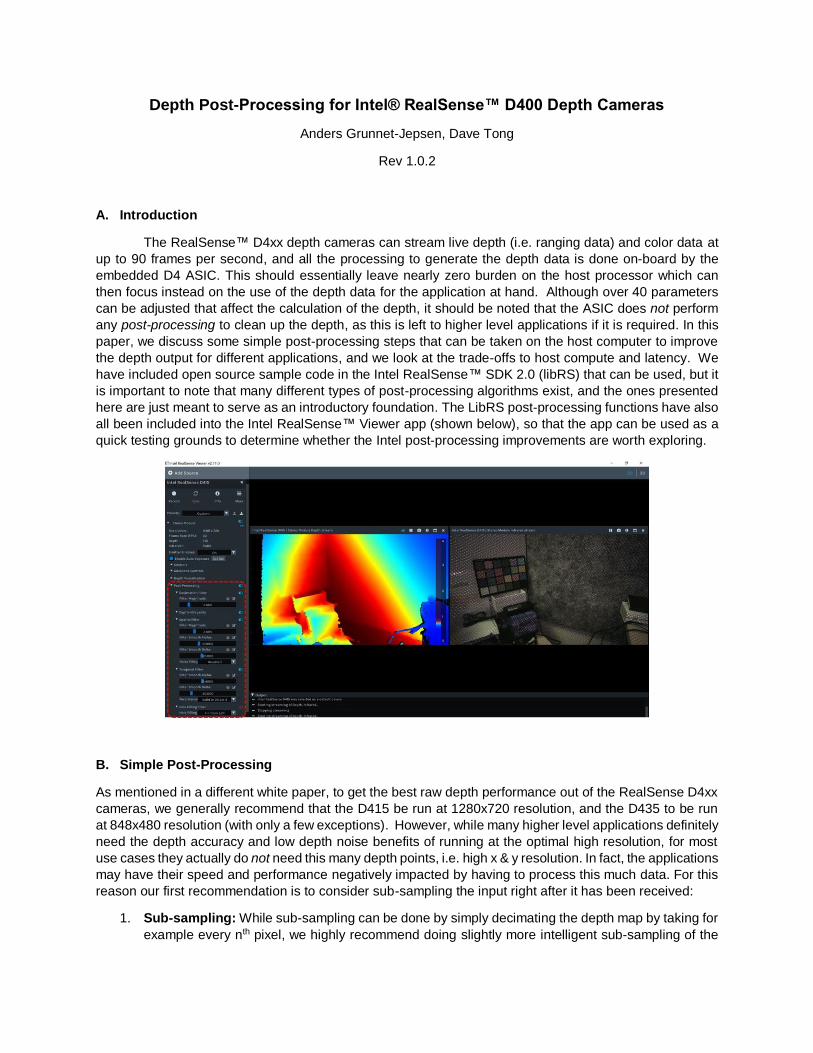
all been included into the Intel RealSense™ Viewer app (shown below), so that the app can be used as a

quick testing grounds to determine whether the Intel post-processing improvements are worth exploring.

B. Simple Post-Processing

As mentioned in a different white paper, to get the best raw depth performance out of the RealSense D4xx

cameras, we generally recommend that the D415 be run at 1280x720 resolution, and the D435 to be run

at 848x480 resolution (with only a few exceptions). However, while many higher level applications definitely

need the depth accuracy and low depth noise benefits of running at the optimal high resolution, for most

use cases they actually do not need this many depth points, i.e. high x & y resolution. In fact, the applications

may have their speed and performance negatively impacted by having to process this much data. For this

reason our first recommendation is to consider sub-sampling the input right after it has been received:

1. Sub-sampling: While sub-sampling can be done by simply decimating the depth map by taking for

example every nth pixel, we highly recommend doing slightly more intelligent sub-sampling of the

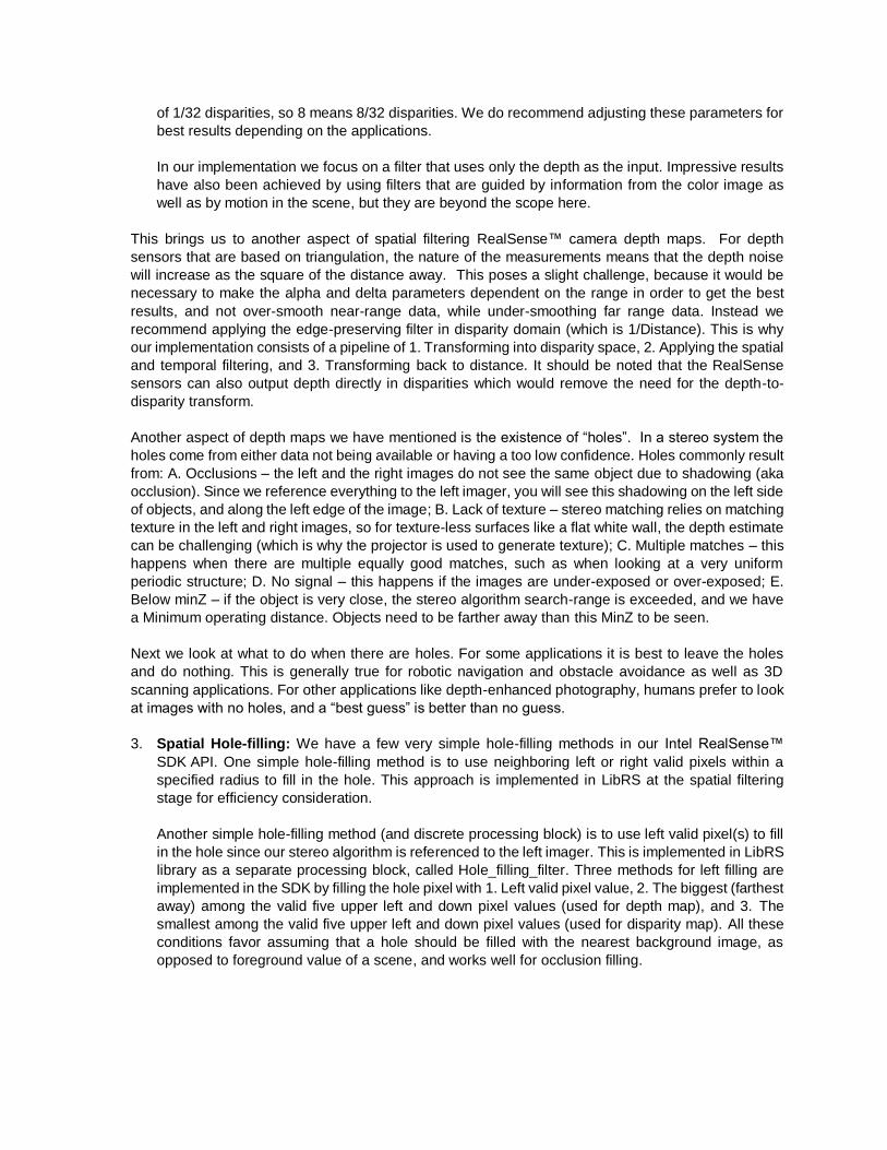
input depth map. We usually suggest using a “non-zero median” or a “non-zero mean” for a pixel

and its nearby neighbors. Considering the computation burden, we suggest using “non-zero

median” for small factor sub-sampling (ex: 2, 3) and “non-zero mean” for large factor sub-sampling

(ex: 4, 5,..). So for example when setting the sub-sampling to 4 (or 4x4), the “non-zero mean”

would entail taking the average of a pixels and its 15 nearest neighbors while ignoring zeroes, and

doing that on an grid subsampled by 4 in the x and y. While this will clearly affect the depth-map x-

y resolution, it should be noted that all stereo algorithms do involve some convolution operations,

so reducing the x-y resolution after capture with modest sub-sampling (<3) will lead to fairly minimal

impact to the depth x-y resolution. A factor of 2 reduction in X-Y resolution should speed

subsequent application processing up by 4x, and a subsampling of 4 should decrease compute by

16x. Moreover, one benefit of the intelligent sub-sampling is it will also do some rudimentary hole-

filling and smoothing of the data using either a “non-zero mean” or “non-zero median” function

(which has a slightly higher computational burden). The “non-zero” refers to the fact that there will

be values on the depth map that are zero that should be ignored. These are “holes” in the depth

map that represent depth data that did not meet the confidence metric, and instead of providing a

wrong value, the camera provides a value of zero at that point. Finally, sub-sampling can actually

help with the visualization of the point-cloud as well because very dense depth maps can be hard

to see unless they are zoomed in.

Once the depth-map has been compressed to a smaller x-y resolution, more complex spatial- and temporal-

filters should be considered. We recommend first considering adding an edge-preserving spatial filter.

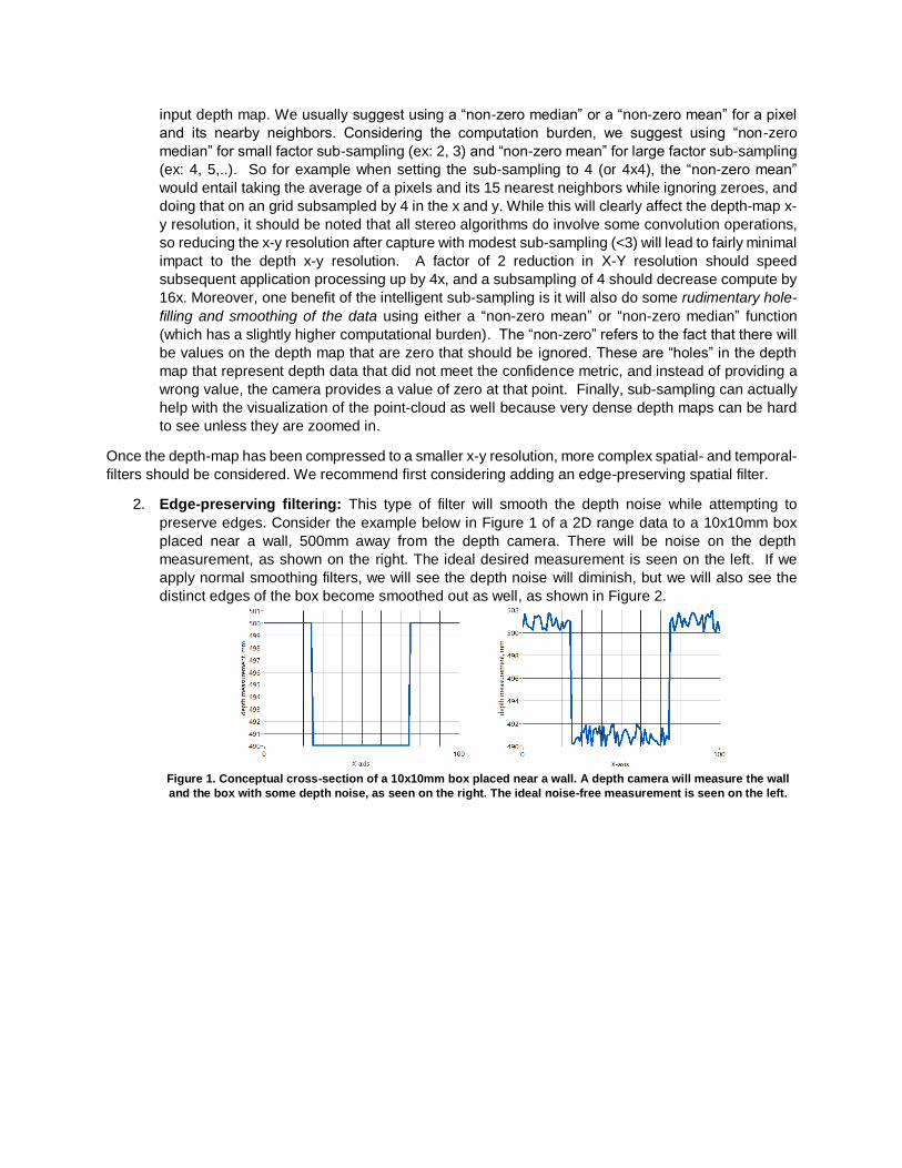
2. Edge-preserving filtering: This type of filter will smooth the depth noise while attempting to

preserve edges. Consider the example below in Figure 1 of a 2D range data to a 10x10mm box

placed near a wall, 500mm away from the depth camera. There will be noise on the depth

measurement, as shown on the right. The ideal desired measurement is seen on the left. If we

apply normal smoothing filters, we will see the depth noise will diminish, but we will also see the

distinct edges of the box become smoothed out as well, as shown in Figure 2.

Figure 1. Conceptual cross-section of a 10x10mm box placed near a wall. A depth camera will measure the wall

and the box with some depth noise, as seen on the right. The ideal noise-free measurement is seen on the left.

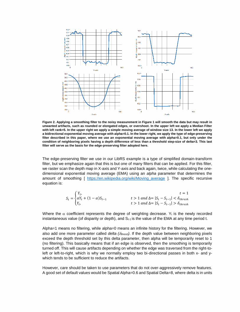
Figure 2. Applying a smoothing filter to the noisy measurement in Figure 1 will smooth the data but may result in

unwanted artifacts, such as rounded or elongated edges, or overshoot. In the upper left we apply a Median Filter

with left rank=5. In the upper right we apply a simple moving average of window size 13. In the lower left we apply

a bidirectional exponential moving average with alpha=0.1. In the lower right, we apply the type of edge-preserving

filter described in this paper, where we use an exponential moving average with alpha=0.1, but only under the

condition of neighboring pixels having a depth difference of less than a threshold step-size of delta=3. This last

filter will serve as the basis for the edge-preserving filter adopted here.

The edge-preserving filter we use in our LibRS example is a type of simplified domain-transform

filter, but we emphasize again that this is but one of many filters that can be applied. For this filter,

we raster scan the depth map in X-axis and Y-axis and back again, twice, while calculating the one-

dimensional exponential moving average (EMA) using an alpha parameter that determines the

amount of smoothing [ https://en.wikipedia.org/wiki/Moving_average ]. The specific recursive

equation is:

𝑆𝑡 = {

𝑌1, 𝑡 = 1

𝛼𝑌𝑡 + (1 − 𝛼)𝑆𝑡−1 𝑡 > 1 𝑎𝑛𝑑 ∆= |𝑆𝑡 − 𝑆𝑡−1| < 𝛿𝑡ℎ𝑟𝑒𝑠ℎ

𝑌𝑡, 𝑡 > 1 𝑎𝑛𝑑 ∆= |𝑆𝑡 − 𝑆𝑡−1| > 𝛿𝑡ℎ𝑟𝑒𝑠ℎ

Where the coefficient represents the degree of weighting decrease. Yt is the newly recorded

instantaneous value (of disparity or depth), and St-1 is the value of the EMA at any time period t.

Alpha=1 means no filtering, while alpha=0 means an infinite history for the filtering. However, we

also add one more parameter called delta (thresh). If the depth value between neighboring pixels

exceed the depth threshold set by this delta parameter, then alpha will be temporarily reset to 1

(no filtering). This basically means that if an edge is observed, then the smoothing is temporarily

turned off. This will cause artifacts depending on whether the edge was traversed from the right-to-

left or left-to-right, which is why we normally employ two bi-directional passes in both x- and y-

which tends to be sufficient to reduce the artifacts.

However, care should be taken to use parameters that do not over-aggressively remove features.

A good set of default values would be Spatial Alpha=0.6 and Spatial Delta=8, where delta is in units

of 1/32 disparities, so 8 means 8/32 disparities. We do recommend adjusting these parameters for

best results depending on the applications.

In our implementation we focus on a filter that uses only the depth as the input. Impressive results

have also been achieved by using filters that are guided by information from the color image as

well as by motion in the scene, but they are beyond the scope here.

This brings us to another aspect of spatial filtering RealSense™ camera depth maps. For depth

sensors that are based on triangulation, the nature of the measurements means that the depth noise

will increase as the square of the distance away. This poses a slight challenge, because it would be

necessary to make the alpha and delta parameters dependent on the range in order to get the best

results, and not over-smooth near-range data, while under-smoothing far range data. Instead we

recommend applying the edge-preserving filter in disparity domain (which is 1/Distance). This is why

our implementation consists of a pipeline of 1. Transforming into disparity space, 2. Applying the spatial

and temporal filtering, and 3. Transforming back to distance. It should be noted that the RealSense

sensors can also output depth directly in disparities which would remove the need for the depth-to-

disparity transform.

Another aspect of depth maps we have mentioned is the existence of “holes”. In a stereo system the

holes come from either data not being available or having a too low confidence. Holes commonly result

from: A. Occlusions – the left and the right images do not see the same object due to shadowing (aka

occlusion). Since we reference everything to the left imager, you will see this shadowing on the left side

of objects, and along the left edge of the image; B. Lack of texture – stereo matching relies on matching

texture in the left and right images, so for texture-less surfaces like a flat white wall, the depth estimate

can be challenging (which is why the projector is used to generate texture); C. Multiple matches – this

happens when there are multiple equally good matches, such as when looking at a very uniform

periodic structure; D. No signal – this happens if the images are under-exposed or over-exposed; E.

Below minZ – if the object is very close, the stereo algorithm search-range is exceeded, and we have

a Minimum operating distance. Objects need to be farther away than this MinZ to be seen.

Next we look at what to do when there are holes. For some applications it is best to leave the holes

and do nothing. This is generally true for robotic navigation and obstacle avoidance as well as 3D

scanning applications. For other applications like depth-enhanced photography, humans prefer to look

at images with no holes, and a “best guess” is better than no guess.

3. Spatial Hole-filling: We have a few very simple hole-filling methods in our Intel RealSense™

SDK API. One simple hole-filling method is to use neighboring left or right valid pixels within a

specified radius to fill in the hole. This approach is implemented in LibRS at the spatial filtering

stage for efficiency consideration.

Another simple hole-filling method (and discrete processing block) is to use left valid pixel(s) to fill

in the hole since our stereo algorithm is referenced to the left imager. This is implemented in LibRS

library as a separate processing block, called Hole_filling_filter. Three methods for left filling are

implemented in the SDK by filling the hole pixel with 1. Left valid pixel value, 2. The biggest (farthest

away) among the valid five upper left and down pixel values (used for depth map), and 3. The

smallest among the valid five upper left and down pixel values (used for disparity map). All these

conditions favor assuming that a hole should be filled with the nearest background image, as

opposed to foreground value of a scene, and works well for occlusion filling.

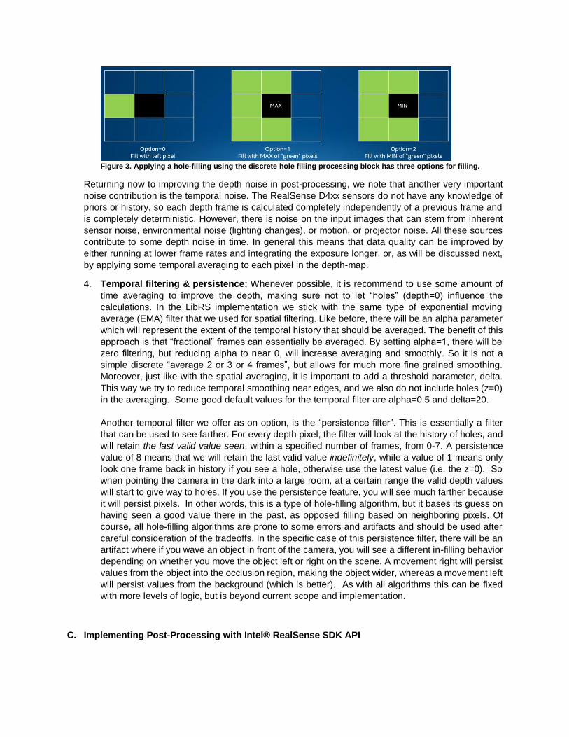
Figure 3. Applying a hole-filling using the discrete hole filling processing block has three options for filling.

Returning now to improving the depth noise in post-processing, we note that another very important

noise contribution is the temporal noise. The RealSense D4xx sensors do not have any knowledge of

priors or history, so each depth frame is calculated completely independently of a previous frame and

is completely deterministic. However, there is noise on the input images that can stem from inherent

sensor noise, environmental noise (lighting changes), or motion, or projector noise. All these sources

contribute to some depth noise in time. In general this means that data quality can be improved by

either running at lower frame rates and integrating the exposure longer, or, as will be discussed next,

by applying some temporal averaging to each pixel in the depth-map.

4. Temporal filtering & persistence: Whenever possible, it is recommend to use some amount of

time averaging to improve the depth, making sure not to let “holes” (depth=0) influence the

calculations. In the LibRS implementation we stick with the same type of exponential moving

average (EMA) filter that we used for spatial filtering. Like before, there will be an alpha parameter

which will represent the extent of the temporal history that should be averaged. The benefit of this

approach is that “fractional” frames can essentially be averaged. By setting alpha=1, there will be

zero filtering, but reducing alpha to near 0, will increase averaging and smoothly. So it is not a

simple discrete “average 2 or 3 or 4 frames”, but allows for much more fine grained smoothing.

Moreover, just like with the spatial averaging, it is important to add a threshold parameter, delta.

This way we try to reduce temporal smoothing near edges, and we also do not include holes (z=0)

in the averaging. Some good default values for the temporal filter are alpha=0.5 and delta=20.

Another temporal filter we offer as on option, is the “persistence filter”. This is essentially a filter

that can be used to see farther. For every depth pixel, the filter will look at the history of holes, and

will retain the last valid value seen, within a specified number of frames, from 0-7. A persistence

value of 8 means that we will retain the last valid value indefinitely, while a value of 1 means only

look one frame back in history if you see a hole, otherwise use the latest value (i.e. the z=0). So

when pointing the camera in the dark into a large room, at a certain range the valid depth values

will start to give way to holes. If you use the persistence feature, you will see much farther because

it will persist pixels. In other words, this is a type of hole-filling algorithm, but it bases its guess on

having seen a good value there in the past, as opposed filling based on neighboring pixels. Of

course, all hole-filling algorithms are prone to some errors and artifacts and should be used after

careful consideration of the tradeoffs. In the specific case of this persistence filter, there will be an

artifact where if you wave an object in front of the camera, you will see a different in-filling behavior

depending on whether you move the object left or right on the scene. A movement right will persist

values from the object into the occlusion region, making the object wider, whereas a movement left

will persist values from the background (which is better). As with all algorithms this can be fixed

with more levels of logic, but is beyond current scope and implementation.

C. Implementing Post-Processing with Intel® RealSense SDK API

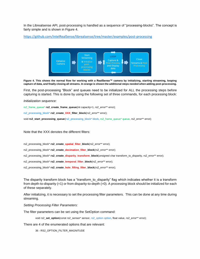
In the Librealsense API, post-processing is handled as a sequence of “processing-blocks”. The concept is

fairly simple and is shown in Figure 4.

https://github.com/IntelRealSense/librealsense/tree/master/examples/post-processing

Figure 4. This shows the normal flow for working with a RealSense™ camera by initializing, starting streaming, looping

capture of data, and finally closing all streams. In orange is shown the additional steps needed when adding post-processing.

First, the post-processing “Block” and queues need to be initialized for ALL the processing steps before

capturing is started. This is done by using the following set of three commands, for each processing block:

Initialization sequence:

rs2_frame_queue* rs2_create_frame_queue(int capacity=1, rs2_error** error);

rs2_processing_block* rs2_create_XXX_filter_block(rs2_error** error);

void rs2_start_processing_queue(rs2_processing_block* block, rs2_frame_queue* queue, rs2_error** error);

Note that the XXX denotes the different filters:

rs2_processing_block* rs2_create_spatial_filter_block(rs2_error** error);

rs2_processing_block* rs2_create_decimation_filter_block(rs2_error** error);

rs2_processing_block* rs2_create_disparity_transform_block(unsigned char transform_to_disparity, rs2_error** error);

rs2_processing_block* rs2_create_temporal_filter_block(rs2_error** error);

rs2_processing_block* rs2_create_hole_filling_filter_block(rs2_error** error);

The disparity transform block has a “transform_to_disparity” flag which indicates whether it is a transform

from depth-to-disparity (=1) or from disparity-to-depth (=0). A processing block should be initialized for each

of these separately.

After initializing, it is necessary to set the processing filter parameters. This can be done at any time during

streaming.

Setting Processing Filter Parameters:

The filter parameters can be set using the SetOption command:

void rs2_set_option(const rs2_sensor* sensor, rs2_option option, float value, rs2_error** error);

There are 4 of the enumerated options that are relevant:

36 - RS2_OPTION_FILTER_MAGNITUDE

37 - RS2_OPTION_FILTER_SMOOTH_ALPHA

38- RS2_OPTION_FILTER_SMOOTH_DELTA

39 - RS2_OPTION_HOLES_FILL

It is important to note that for the “sensor” pointer in set_option, it should instead be the pointer to the

specific “Processing Block”. So for example, if we want to set the ALPHA parameter for the temporal filter,

we would use the pointer to the temporal filter block.

For the decimation block the only option needed is:

Filter magnitude = sub-sampling number (ex: 2, 3, 4..)

For the spatial filter block there are four options:

Filter magnitude = iterations of the filter. We recommend using 2 (default).

Filter smooth alpha = the spatial alpha parameters (0-1)

Filter smooth delta = the spatial delta threshold in 1/32 disparities. Default is 20, but try 8 as well.

Filter holes fill = the spatial radius for hole filling (0=none, 1=2 pixels, 2=4 pixels, 3=8 pixels, 4=16 pixels, 5=unlimited).

For the temporal filter block the 3 options are:

Filter smooth alpha = the temporal alpha parameters (0-1)

Filter smooth delta = the temporal delta threshold in 1/32 disparities. Default is 20.

Filter holes fill = the persistence value (0=no persistence, and 8=persist indefinitely)

For the separate hole-filling block there is only one option:

Filter holes fill = additional filling of holes based on choosing nearest neighbor filled with 0=Use left pixel to fill, 1=Max of

nearest pixels on left, and 2=Min value of nearest pixels on left, as shown in Figure 3.

Once all the filters have been initialized, we have nice flexibility in how we process a frame during streaming.

The normal flow of capturing data in a loop is to use the wait_for_frame command.

rs2_frame* rs2_wait_for_frame(rs2_frame_queue* queue, unsigned int timeout_ms, rs2_error** error);

This is a blocking call. As soon as a new frame arrives, this frame can be analyzed and the data can be

dispositioned and displayed, before the frame is released, and the process is repeated.

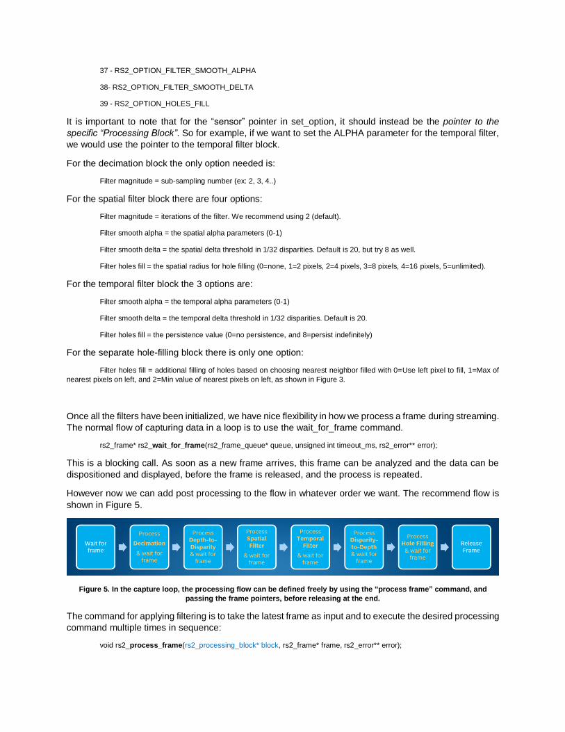
However now we can add post processing to the flow in whatever order we want. The recommend flow is

shown in Figure 5.

Figure 5. In the capture loop, the processing flow can be defined freely by using the “process frame” command, and

passing the frame pointers, before releasing at the end.

The command for applying filtering is to take the latest frame as input and to execute the desired processing

command multiple times in sequence:

void rs2_process_frame(rs2_processing_block* block, rs2_frame* frame, rs2_error** error);

where the processing block pointer specifies the specific post-processing step. The output frame from each

step will then be the input frame to the next processing block, and so on. Only the final processed frame

needs to be released before repeating the loop.

D. Example Results and trade-offs

We now turn to exploring a few examples, the effects of the settings, as well as the computational burden.

First we address the question of the computational burden. Figure 6 shows a breakdown of the time it takes

to complete each step, in milliseconds, and on Intel i7 laptop. We benchmark here only for one PC in order

to show the relative processing times of the filters. Clearly these times will be dependent on the specific

compute platform being used.

Figure 6. This details the time it takes to perform post-processing on a two different PC platforms. This is meant primarily to

give some insight into where the main processing burden is. These are all done assuming single threaded implementation

on the CPU.

By adjusting the subsampling number from 1 (no-subsampling) to 6, we see that total processing time is

reduced from 37ms to 5.5ms. We also see that the spatial filter is the most time-consuming for low

subsample (high output resolution), but for high subsample (low output resolution) the spatial filtering time

is reduced from 22ms to 1.34ms. It should also be noted that these filters have not been optimized by any

use of special instruction or parallel processing, so as to keep the code portability as high as possible. For

many applications the best trade-off is likely to be a sub-sampling of 3 when starting with 1280x720

resolution which, without the use of hole-filling, takes 12.5ms for all post-processing.

The temporal filter is seen to be quite efficient, and uses only a single full frame of memory. At a sub-sample

factor of 3 (taking 5.8ms), the temporal filter takes only 0.76ms, irrespective of the filter alpha or delta

parameter choice.

Turning now to the effect of the filters, we will show some qualitative results for a specific single scene. The

test scene is shown in Figure 7. It is a white RealSense packaging box, and a black leather notebook on a

flat textured surface.

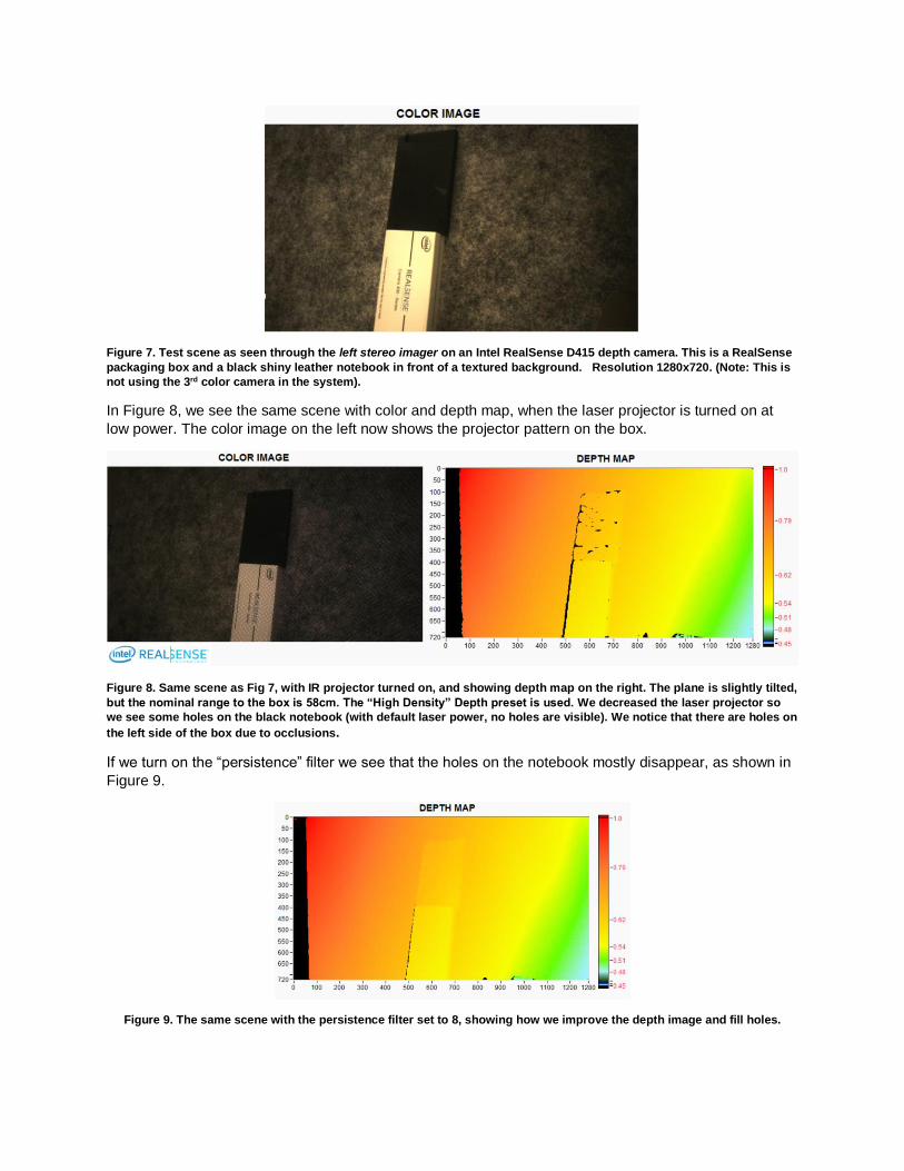
Figure 7. Test scene as seen through the left stereo imager on an Intel RealSense D415 depth camera. This is a RealSense

packaging box and a black shiny leather notebook in front of a textured background. Resolution 1280x720. (Note: This is

not using the 3rd color camera in the system).

In Figure 8, we see the same scene with color and depth map, when the laser projector is turned on at

low power. The color image on the left now shows the projector pattern on the box.

Figure 8. Same scene as Fig 7, with IR projector turned on, and showing depth map on the right. The plane is slightly tilted,

but the nominal range to the box is 58cm. The “High Density” Depth preset is used. We decreased the laser projector so

we see some holes on the black notebook (with default laser power, no holes are visible). We notice that there are holes on

the left side of the box due to occlusions.

If we turn on the “persistence” filter we see that the holes on the notebook mostly disappear, as shown in

Figure 9.

Figure 9. The same scene with the persistence filter set to 8, showing how we improve the depth image and fill holes.

If we instead turn on the spatial filter hole-filling block we see that the holes near the box and notebook

disappear and are replaced by background. While this in-filling appears to work well in the middle of the

notebook and for the occlusions near the RealSense box, near the edges of the notebook we see that the

holes have been replaced with the depth from the background leaving the impression of a badly torn

notebook. For many applications it may be better to leave a hole, than to give false values.

Figure 10. Using simple “Hole fill” (left in-fill), also removes all holes, but tends to add some artifacts, like the book having

background holes.

For the rest of this paper we will focus on the point-cloud visualization, which is the best approach to viewing

spatial noise, especially if we do not apply color image texture to the mesh which can tend to hide data. As

a starting reference point, we measure the background tilted plane-fit RMS noise on a small patch near the

right of the box. The RMS noise is about 0.6mm, or 0.085 subpixel RMS noise, with the projector off. With

the projector turned on at 70mW (lower than default of 150mW), this actually degrades to 0.7mm or 0.1

sub-pixel RMS noise (see our other tuning paper for why this is the case).

Figure 11 shows the simple un-textured point cloud for subsampling of 1 (none), 2, 3.

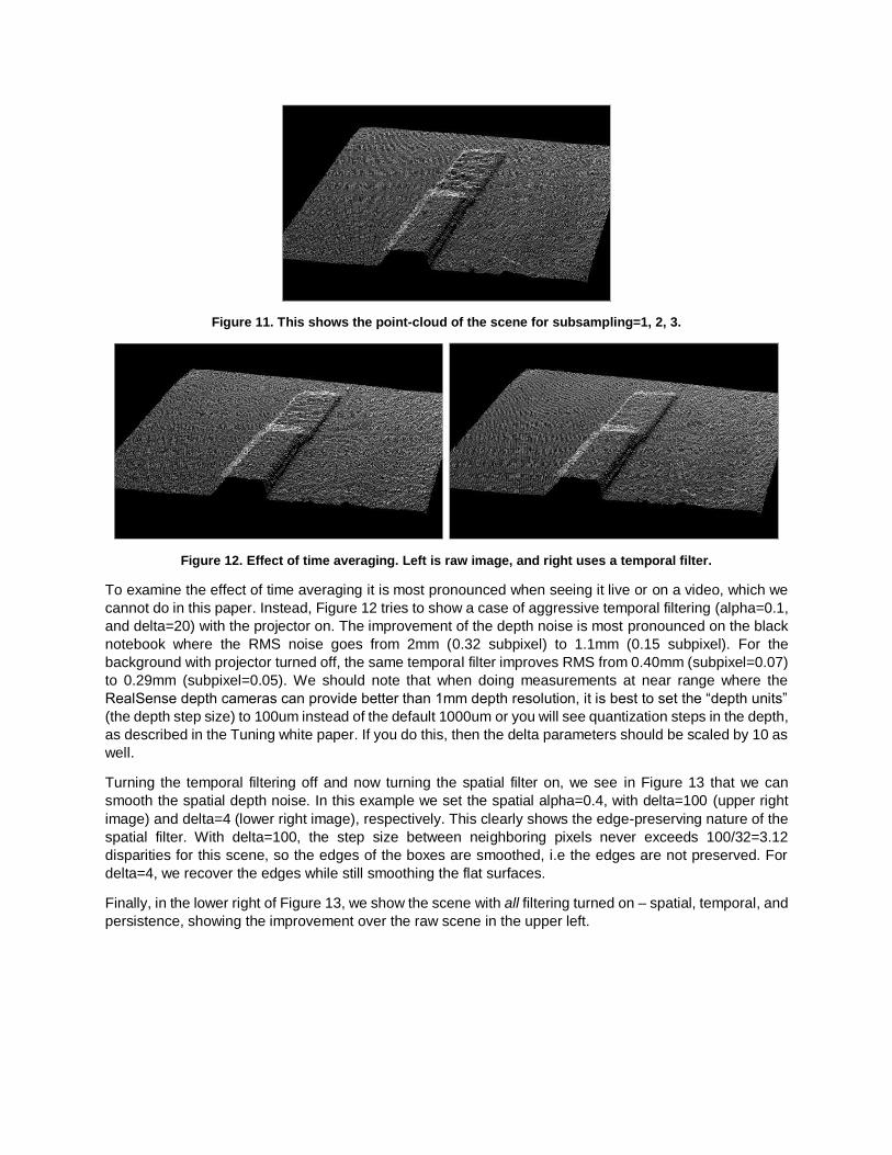
Figure 11. This shows the point-cloud of the scene for subsampling=1, 2, 3.

Figure 12. Effect of time averaging. Left is raw image, and right uses a temporal filter.

To examine the effect of time averaging it is most pronounced when seeing it live or on a video, which we

cannot do in this paper. Instead, Figure 12 tries to show a case of aggressive temporal filtering (alpha=0.1,

and delta=20) with the projector on. The improvement of the depth noise is most pronounced on the black

notebook where the RMS noise goes from 2mm (0.32 subpixel) to 1.1mm (0.15 subpixel). For the

background with projector turned off, the same temporal filter improves RMS from 0.40mm (subpixel=0.07)

to 0.29mm (subpixel=0.05). We should note that when doing measurements at near range where the

RealSense depth cameras can provide better than 1mm depth resolution, it is best to set the “depth units”

(the depth step size) to 100um instead of the default 1000um or you will see quantization steps in the depth,

as described in the Tuning white paper. If you do this, then the delta parameters should be scaled by 10 as

well.

Turning the temporal filtering off and now turning the spatial filter on, we see in Figure 13 that we can

smooth the spatial depth noise. In this example we set the spatial alpha=0.4, with delta=100 (upper right

image) and delta=4 (lower right image), respectively. This clearly shows the edge-preserving nature of the

spatial filter. With delta=100, the step size between neighboring pixels never exceeds 100/32=3.12

disparities for this scene, so the edges of the boxes are smoothed, i.e the edges are not preserved. For

delta=4, we recover the edges while still smoothing the flat surfaces.

Finally, in the lower right of Figure 13, we show the scene with all filtering turned on – spatial, temporal, and

persistence, showing the improvement over the raw scene in the upper left.

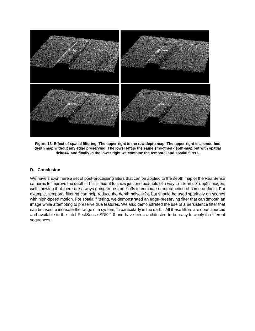
Figure 13. Effect of spatial filtering. The upper right is the raw depth map. The upper right is a smoothed

depth map without any edge preserving. The lower left is the same smoothed depth-map but with spatial

delta=4, and finally in the lower right we combine the temporal and spatial filters.

D. Conclusion

We have shown here a set of post-processing filters that can be applied to the depth map of the RealSense

cameras to improve the depth. This is meant to show just one example of a way to “clean up” depth images,

well knowing that there are always going to be trade-offs in compute or introduction of some artifacts. For

example, temporal filtering can help reduce the depth noise >2x, but should be used sparingly on scenes

with high-speed motion. For spatial filtering, we demonstrated an edge-preserving filter that can smooth an

image while attempting to preserve true features. We also demonstrated the use of a persistence filter that

can be used to increase the range of a system, in particularly in the dark. All these filters are open sourced

and available in the Intel RealSense SDK 2.0 and have been architected to be easy to apply in different

sequences.