978-1-4244-7493-6/10/$26.00 ©2010 IEEE ICME 2010

DEPTH-LEVEL-ADAPTIVE VIEW SYNTHESIS FOR 3D VIDEO

Ying Chen1, Weixing Wan2, Miska M. Hannuksela3, Jun Zhang2, Houqiang Li2, and Moncef Gabbouj1

1Department of Signal Processing, Tampere University of Technology

2University of Science and Technology of China 3Nokia Research Center

chenyingtmm@gmail.com libra@mail.ustc.edu.cn

miska.hannuksela@nokia.com zhagjun@mail.ustc.edu.cn

lihq@ustc.edu.cn moncef.gabbouj@tut.fi

ABSTRACT

In the multiview video plus depth (MVD) representation for 3D video, a depth map sequence is coded for each view. In the decoding end, a view synthesis algorithm is used to generate virtual views from depth map sequences. Many of the known view synthesis algorithms introduce rendering artifacts especially at object boundaries. In this paper, a depth-level-adaptive view synthesis algorithm is presented to reduce the amount of artifacts and to improve the quality of the synthesized images. The proposed algorithm introduces awareness of the depth level so that no pixel value in the synthesized image is derived from pixels of more than one depth level. Improvements on objective quality of the synthesized views were achieved in five out of eight test cases, while the subjective quality of the proposed method was similar to or better than that of the view synthesis method used by Moving Picture Experts Group (MPEG).

Keywords—3D video, View Synthesis, Multiview Video plus Depth (MVD)

1. INTRODUCTION With recent advances in the acquisition and display technologies, 3D video is becoming a reality in the consumer domain with different application opportunities. 3D video has gained a wide interest recently in the consumer electronics industry and the standard committees. Typical 3D video applications are 3D television (TV) and free viewpoint video. 3D TV refers to the extension of traditional 2D TV with capability of 3D rendering. In this application, more than one view is decoded and displayed simultaneously [1]. In free-viewpoint video applications, the viewer can interactively choose the viewpoint in a 3D space to observe a real-world scene from preferred

perspectives [2][3]. Different formats can be used for 3D video. A straightforward representation is to have multiple 2D videos for each viewing angle or position, e.g., with H.264/AVC [4], or MVC, the multiview extension of H.264/AVC [5]. Another representation of 3D video is to have a single-view texture video with the associated depth map, out of which virtual views can be generated using depth-image-based rendering (DIBR) [6]. The drawback of this solution is there are occlusions and pinholes in the virtual views. To improve the rendering quality, multiview video plus depth (MVD) was proposed, which represents the 3D video content with not only texture videos but also depth map videos for multiple views [7]. MPEG has been investigating 3D video compression techniques as well as depth estimation and view synthesis in the 3D video (3DV) ad-hoc group [8].

Generating virtual views is useful in the two typical use cases mentioned above. In free-viewpoint video, smooth navigation requires generating of virtual views in any view angle, to provide the flexibility and interactivity. In 3D TV, typically several views can be transmitted while more views can be synthesized, to reduce the bandwidth consumption of transmitting a full set of views. Moreover, the most comfortable view disparity for a particular display might not match the camera separation in a coded bitstream. Consequently, generation of virtual views might be preferred to obtain a comfortable view disparity for a display and particular viewing conditions.

A typical 3D video transmission system is shown in Fig. 1. 3D video content is coded into the MVD format at the encoder side. The depth maps of multiple views may need to be generated by depth estimation. At the decoder side, multiple views with depth maps are firstly decoded, and then a desired virtual view can be interpolated by view synthesis. Real-time generation of virtual views makes smooth view navigation and 3D rendering possible, e.g., in a stereo fashion when the two view angles are selected.

1724978-1-4244-7492-9/10/$26.00 ©2010 IEEE ICME 2010

Although differing in details, most of the view synthesis algorithms utilize 3D warping based on explicit geometry, i.e., depth images [9]. McMillan’s approach [10] uses a non-Euclidean formulation of the 3D warping, which is efficient under the condition that the camera parameters are unknown or the camera calibration is poor. Mark’s approach [11], however, strictly follows Euclidean formulation, assuming the camera parameters for the acquisition and view interpolation are known.

Occlusions, pinholes, and reconstruction errors are the most common artifacts introduced in the 3D warping process [11]. These artifacts occur more frequently in the object edges, where pixels with different depth levels may be mapped to the same pixel location of the virtual image. When those pixels are averaged to reconstruct the final pixel value for the pixel location in the virtual image, an artifact might be generated, because pixels with different depth levels usually belong to different objects. To avoid the problem, a depth-level-adaptive view synthesis algorithm is introduced in this paper. During the view synthesis, depth values are firstly classified into different levels; then only the pixels with depth values in a certain depth level are considered for the visibility problem, the pinhole filling, and the reconstruction.

The proposed method is suitable for low-complexity view synthesis solutions, such as ViSBD (View Synthesis Based on Disparity/Depth) [12][13] was adopted as a reference software in the MPEG 3DV ad-hoc group. ViSBD follows the pinhole camera model and takes the camera parameters as well as the per-pixel depth as input, as assumed in Mark’s approach [11]. Compared to the synthesis results of ViSBD, a noticeable luma Peak Signal-to-Noise Ratio (PSNR) gain as well as subjective quality improvements can be observed under the test conditions of MPEG 3DV.

This paper is organized as follows. In Section 2, the ViSBD view synthesis technique is introduced. Section 3 presents the proposed view synthesis algorithm, with improved approaches for visibility, hole filling, and reconstruction, based on clustered depth. Experimental results are given in Section 4. Section 5 concludes the paper.

2. VISBD VIEW SYNTHESIS

Since April 2008, the MPEG 3DV ad-hoc group has been devoted to Exploration Experiments (EE) evaluating depth generation and view synthesis techniques. As a result of the EEs, a view synthesis reference software module [14] has been developed. It integrates two software pieces, one developed by Nagoya University [15] and ViSBD developed by Thomson [12][13]. ViSBD, however, is stand-alone and requires less computational power. It was therefore selected as the basis of our work and the most relevant part of it are reviewed in the following sub-sections. 2.1. Warping 3D warping maps a pixel of a reference view to a destination pixel of a virtual view. Three different coordinate systems are involved in a general case: the world coordinate system, the camera coordinate system, and the image coordinate system [16]. A pixel, with coordinate (ur, vr) in an image plane of the reference view and its depth value z, is projected to a world coordinate and re-projected to the virtual view with the coordinate of (uv, vv). In the image plane, the principal point is the intersection point of the optical axis and the image plane. The principal point and the origin of the image plane can be the same. The offset between the principal point and the origin is called the principal point offset.

In the MPEG 3DV EEs, it is assumed that all cameras are in 1D parallel arrangement. As discussed in [17], the 3D warping formula can be simplified as: ⁄ (1)

wherein f is the focal length of the camera parameters, T is the (horizontal) translation between these two cameras, Od is the difference of the principal point offsets of the two cameras, and dis is the disparity of the pixel pair in the two image planes. There is no vertical disparity and vv = vr.

Note that the depth values are quantized into a limited dynamic range with 8 bits: 0 to 255. The utilized conversion formula from the 8-bit depth value d to the depth (z) in the real-world coordinates is: 1 (2)

wherein [znear, zfar] is the depth range of the physical scene. Note that the closer depth is in the real-world coordinate system, the larger quantized depth value becomes.

A pixel in the reference view cannot always be mapped one-to-one to a pixel in the virtual view and thus two issues need to be resolved: visibility and hole filling. In this paper, the pixel position in the reference view with a coordinate of (ur, vr) is called a original pixel position and the respective pixel position with the coordinate of (uv, vv) in the virtual view is called a mapped pixel position. 2.2. Visibility When multiple pixels of a reference view are mapped to the same pixel location of a virtual view, those candidate pixels

Fig. 1. 3D video transmission system.

1725

need to be combined, e.g., by competition or weighting. In ViSBD, a competition approach based on z-buffering is utilized. During the 3D warping, a z-buffer is maintained for each pixel position in a reference view. When a pixel in a reference view is warped to a target view, the coordinates of the mapped pixel are rounded to the nearest integer pixel position. If no pixel has been warped to the mapped pixel position earlier, the pixel of the reference view is copied to the mapped pixel and the respective z-buffer value takes the depth value of the pixel in the reference view. Otherwise, if the pixel in the reference view is closer to the camera than the pixel warped earlier to the same mapped pixel position, the sample value of the mapped pixel position and the respective z-buffer value are overwritten by the original pixel value and the depth value of the original pixel, respectively. This way, the sample value of a pixel location p in the virtual view is always set as the value of the pixel which has the largest depth value among the pixels that are mapped to p.

2.3. Blending To solve the occlusion problem, multiple (typically two) views are utilized as reference views. For example, occlusions may occur at the right of an object if the reference view is from the left. In such a case, the view on the right can provide a good complement.

In the view synthesis process, two prediction images are warped, one from the left view and another one from the right view. The two prediction images are then blended to form one synthesized image. The blending process is described in the following paragraphs.

When there is no hole in the same pixel location in neither of the prediction images, the pixel value in the synthesized image is formed by averaging the respective pixel values in the prediction images in a weighted manner based on the camera distances. The weights for the left view and right view prediction images are: / , ⁄ (3)

wherein lR and lL are the camera distances from the virtual view to the right view and to the left view, respectively.

When only one pixel in the same pixel location in the prediction images is a hole, the respective pixel in the synthesized image is set to the pixel value which does not correspond to a hole. When the same pixel location in both of the prediction images contains a hole, the hole filling process described in Section 2.4 is performed. 2.4. Hole Filling When pixels are occluded in the virtual view because of a perspective change and no pixel is mapped to a pixel

position in a virtual view, a hole is generated. Holes are filled by the neighboring pixels belonging to the background. A pixel is identified as a background pixel if its depth value is smaller than the depth values of all neighboring pixels. In 1D parallel camera arrangement, however, the neighboring pixels for a hole pixel are constrained along the horizontal direction, i.e., to the pixel on the left and right side of the hole. The neighboring pixel identified as a background pixel is used to fill the hole.

3. DEPTH-LEVEL-ADAPTIVE VIEW SYNTHESIS In view synthesis, it is usually necessary to consider multiple candidate pixels for generating the intensity value of a destination pixel in the virtual view. However, when the candidate pixels belong to different objects, the destination pixel might be blurred. To address this issue, we proposed a depth-level-adaptive view synthesis algorithm, which prevents mixing pixels from different depth levels. The algorithm first classifies depth pixels in clusters based on their depth value. The depth clustering algorithm is presented in details in Section 3.1. Then, the depth clusters are utilized in visibility resolving and blending as described in Section 3.2. Finally, any remaining holes are filled in a depth-adaptive manner as presented in Section 3.3. 3.1. Depth Clustering In this paper, it is assumed that pixels having similar depth values within in a small region belong to the same object. In order to utilize this assumption in the view synthesis process, a novel clustering algorithm based on the K-means-method [18] is applied to cluster the depth values into the K clusters. The details of the clustering algorithm are explained in the remaining of this sub-section.

Without loss of generality, assume there is K clusters in each step of the following clustering algorithm and are the depth samples in cluster i, is the centroid of a cluster i and its Sum of Absolute Error (SAE) is calculated as ∑ || ||.

1. At the beginning, set the number of clusters K to 1, i.e., there is only one cluster enclosing all the depth values. Moreover, set a control variable L to 0.

2. Calculate the Sum of Absolute Error (SAE) of each cluster as , 1,2, , . Denote ∑ .

3. Select cluster m that has the maximum SAE. Split cluster m, into two new clusters. The two new clusters have the centroids of and .

4. Use the K-means algorithm to update the new K+1 clusters. Calculate .

1726

5. If | |, , , wherein R is a

threshold to determine the fluctuation between SumN+1 and SumN, then increase L by 1 and go to step 6. Else set L to 0, increase K by 1, and go to step 2.

6. If L>Length, terminate the depth clustering. Else increase K by 1 and go to step 2.

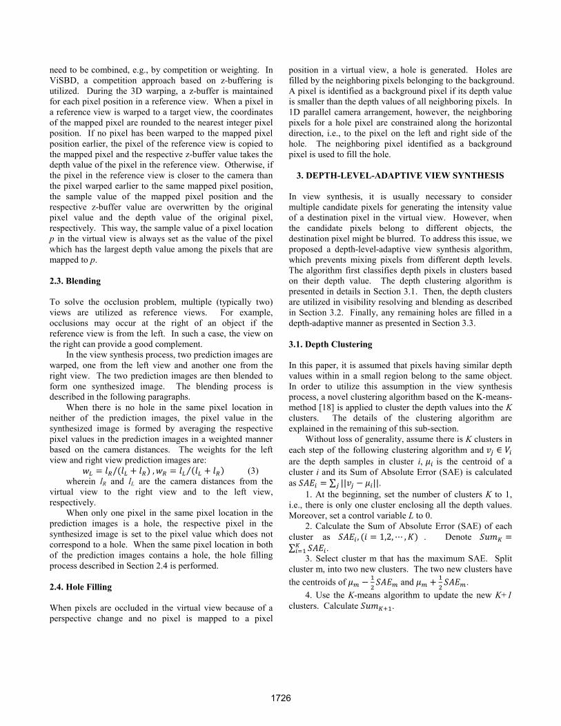
Fig. 2 shows an example image where the algorithm generated six depth clusters and the depth of each pixel is replaced by the centroid of the cluster it belongs to.

Assume the centroids of the depth clusters are , and the depth values are distributed in the

closed intervals without overlap: , , , wherein , 1 corresponds to a depth level, which has the depth value of as the centroid. Note that the depth values are in the quantized 8-bit domain. 3.2. Depth-level-aware Visibility and Blending The Z-buffering method of ViSBD only uses the candidate pixel with the maximum depth value. Pixels with much larger depth values are not helpful and can blur the details of the synthesized image. However, averaging of candidate pixels with similar depth values may increase the quality of the synthesized image.

Consider an integer pixel location (u, v) in the virtual view, the set of mapped pixel considered for the visibility is in a window with a size of W×W, described as follows:

x, y | | | W 2⁄ , | | W 2⁄ (4) , which is a union of the subsets with different depth levels: , , , (5)

wherein is the depth value of a pixel (x, y). The visibility problem is resolved by using only those

candidate pixels which are in the W×W window and belong to the depth cluster having the greatest depth value within the window, i.e., the pixels in a visible pixel set , where s is the greatest value corresponding to a non-empty set. If the visible pixel set contains multiple candidate pixels, the candidate pixels are averaged to reconstruct the final pixel value. If the visible pixel set contains no candidate pixels, hole filling is applied as described in Section 3.3.

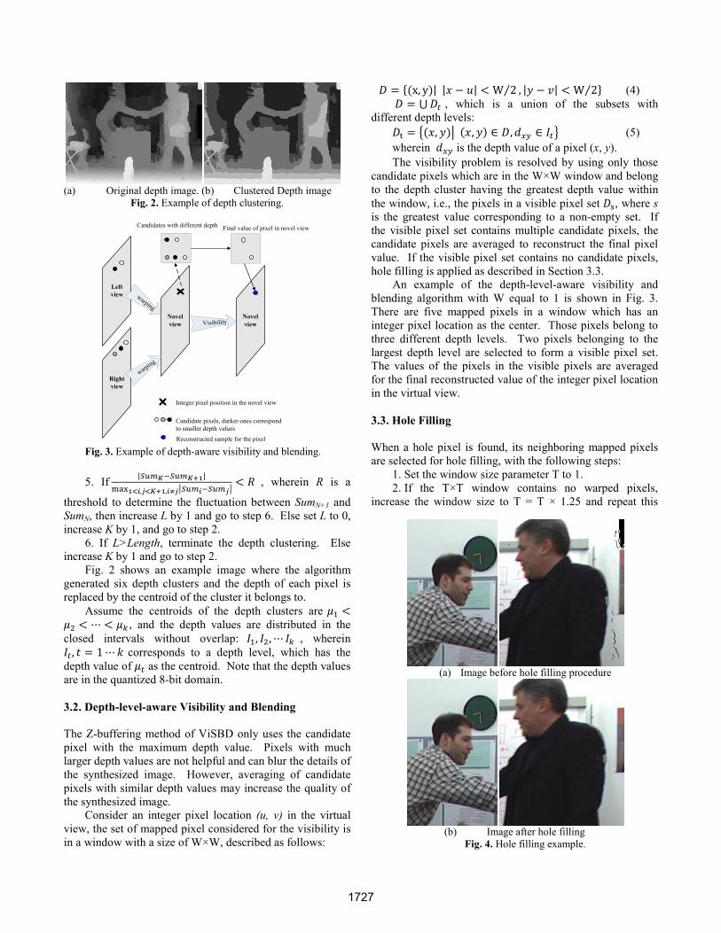
An example of the depth-level-aware visibility and blending algorithm with W equal to 1 is shown in Fig. 3. There are five mapped pixels in a window which has an integer pixel location as the center. Those pixels belong to three different depth levels. Two pixels belonging to the largest depth level are selected to form a visible pixel set. The values of the pixels in the visible pixels are averaged for the final reconstructed value of the integer pixel location in the virtual view. 3.3. Hole Filling When a hole pixel is found, its neighboring mapped pixels are selected for hole filling, with the following steps:

1. Set the window size parameter T to 1. 2. If the T×T window contains no warped pixels,

increase the window size to T = T × 1.25 and repeat this

(a) Original depth image. (b) Clustered Depth image Fig. 2. Example of depth clustering.

Right view

Novel view

Left view

Novel view

warping

warping

Visibility

Candidates with different depth Final value of pixel in novel view

Candidate pixels, darker ones correspond to smaller depth values

Integer pixel position in the novel view

Reconstructed sample for the pixel

Fig. 3. Example of depth-aware visibility and blending.

(a) Image before hole filling procedure

(b) Image after hole filling

Fig. 4. Hole filling example.

1727

step. 3. Derive the set of mapped pixels considered for

hole filling from the warped pixels in the T×T window. 4. Assume and split into , wherein the

subsets contain pixels belonging to different depth levels, similarly to equation (5).

5. Select that contains more candidate pixels than any other .

6. Average the values of the pixels in to fill the hole.

Fig. 4 shows an example of the proposed hole filling.

4. EXPERIMENTAL RESULTS The proposed algorithm was implemented on top of and compared with ViSBD version 2.1 [12]. Half-pixel accuracy in view synthesis (configuration parameters UpsampleRefs and SubPelOption were set to 2 and 1, respectively) and boundary-aware splatting (SplattingOption was set to 2) were used in ViSBD 2.1, as these options were found to provide good results. Four sequences were tested in the experiments: LeavingLaptop, BookArrival, Dog, and Pantomime. For each sequence, two views were selected as reference views and two views in the middle were generated. The view identifiers of the reference views and the generated views are listed in Table 1.

Table 1. Reference view and novel view identifiers

Sequence Left View Right View Novel Views LeavingLaptop 10 7 9, 8

BookArrival 10 7 9, 8 Dog 38 42 39, 41

Pantomime 38 41 39, 40 In the proposed depth clustering method, parameters R

and Length affect the computational complexity and the clustering accuracy: the smaller R and the larger Length, the more accurate clustering result and the heavier computational complexity. Values of R and Length were tested empirically, and eventually 4% and 6 were selected for R and Length, respectively. In addition, the window size W in visibility determination and blending (Section 3.2) was set to 1 and the window size T in hole filling (Section 3.3) was initialized to 1.0.

We investigated the objective quality measured in terms of average luma PSNR of the synthesized views. The objective results are reported in Section 4.1. However, it is known that PSNR is not an accurate metric for measuring the subjective quality of synthesized views, and hence the subjective quality was evaluated and reported in Section 4.2. 4.1. PSNR results Average luma PSNR values were calculated between a synthesized view and the corresponding original view. For

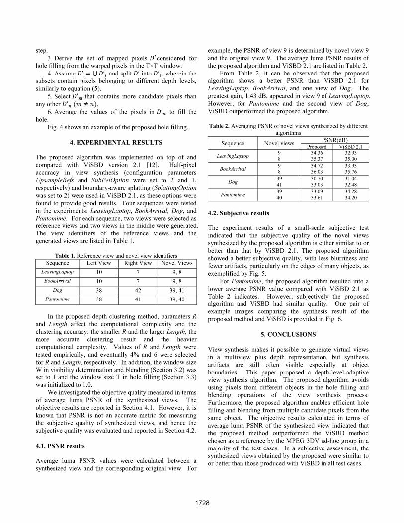
example, the PSNR of view 9 is determined by novel view 9 and the original view 9. The average luma PSNR results of the proposed algorithm and ViSBD 2.1 are listed in Table 2.

From Table 2, it can be observed that the proposed algorithm shows a better PSNR than ViSBD 2.1 for LeavingLaptop, BookArrival, and one view of Dog. The greatest gain, 1.43 dB, appeared in view 9 of LeavingLaptop. However, for Pantomime and the second view of Dog, ViSBD outperformed the proposed algorithm. Table 2. Averaging PSNR of novel views synthesized by different

algorithms

Sequence Novel views PSNR(dB) Proposed ViSBD 2.1

LeavingLaptop 9 8

34.36 35.37

32.93 35.00

BookArrival 9 8

34.72 36.03

33.93 35.76

Dog 39 41

30.70 33.03

31.04 32.48

Pantomime 39 40

33.09 33.61

34.28 34.20

4.2. Subjective results The experiment results of a small-scale subjective test indicated that the subjective quality of the novel views synthesized by the proposed algorithm is either similar to or better than that by ViSBD 2.1. The proposed algorithm showed a better subjective quality, with less blurriness and fewer artifacts, particularly on the edges of many objects, as exemplified by Fig. 5.

For Pantomime, the proposed algorithm resulted into a lower average PSNR value compared with ViSBD 2.1 as Table 2 indicates. However, subjectively the proposed algorithm and ViSBD had similar quality. One pair of example images comparing the synthesis result of the proposed method and ViSBD is provided in Fig. 6.

5. CONCLUSIONS View synthesis makes it possible to generate virtual views in a multiview plus depth representation, but synthesis artifacts are still often visible especially at object boundaries. This paper proposed a depth-level-adaptive view synthesis algorithm. The proposed algorithm avoids using pixels from different objects in the hole filling and blending operations of the view synthesis process. Furthermore, the proposed algorithm enables efficient hole filling and blending from multiple candidate pixels from the same object. The objective results calculated in terms of average luma PSNR of the synthesized view indicated that the proposed method outperformed the ViSBD method chosen as a reference by the MPEG 3DV ad-hoc group in a majority of the test cases. In a subjective assessment, the synthesized views obtained by the proposed were similar to or better than those produced with ViSBD in all test cases.

1728

6. REFERENCES

[1] A. Vetro, W. Matusik, H. Pfister, and J. Xin, “Coding Approaches for end-to-end 3D TV systems,” Picture Coding Symposium, PCS’04, pp. 319–324, San Francisco, CA, USA, Dec. 2004. [2] H. Kimata, M. Kitahara, K. Kamikura, Y. Yashima, T. Fujii, and M. Tanimoto, “System Design of Free Viewpoint Video Communication,” International Conference on Computer and Information Technology, CIT, 2004. [3] A. Smolic and P. Kauff, “Interactive 3-D Video Representation and Coding Technologies,” Proceedings of the IEEE, vol. 93, no. 1, pp. 98–110, 2005. [4] T. Wiegand, G.J. Sullivan, G. Bjøntegaard and A. Luthra, “Overview of the H.264/AVC Video Coding Standard,” IEEE Transactions on Circuits and Systems for Video Technology, vol. 13, no. 7, Jul. 2003. [5] Y. Chen, Y.-K. Wang, K. Ugur, M.M. Hannuksela, J. Lainema, and M. Gabbouj, “The emerging MVC standard for 3D video services,” EURASIP Journal on Advances in Signal Processing, vol. 2009, Article ID 786015, 13 pages, doi:10.1155/2009/786015. [6] C. Fehn, “Depth-Image-Based Rendering (DIBR), Compression and Transmission for a New Approach on 3D-TV,” Proceedings of SPIE Stereoscopic Displays and Virtual Reality Systems XI, pp. 93–104, San Jose, CA, USA, Jan. 2004. [7] A. Smolic, K. Müller, K. Dix, P. Merkle, P. Kauff, and T. Wiegand, “Intermediate View Interpolation Based on Multiview Video Plus Depth for Advanced 3D Video Systems,” Proc. ICIP 2008, IEEE International Conference on Image Processing, San Diego, CA, USA, Oct. 2008. [8] “Vision on 3D Video,” ISO/IEC JTC1/SC29/WG11, MPEG document N10357, Feb. 2009. [9] H.-Y. Shum, S.B. He, and S.-C. Chan, “Survey of image-based representations and compression techniques,” IEEE Transactions

on Circuits and Systems for Video Technology, vol. 13, no. 11, pp. 1020–1037, Nov. 2003. [10] L. McMillan, “An Image-Based Approach to Three-Dimensional Computer Graphics,” PhD thesis, University of North Carolina at Chapel Hill, Chapel Hill, NC, USA, 1997. [11] W. R. Mark, “Post-Rendering 3D Image Warping: Visibility, Reconstruction, and Performance for Depth-Image Warping,” PhD thesis, University of North Carolina at Chapel Hill, Chapel Hill, NC, USA, Apr.1999. [12] D. Tian, P. Pandit, and C. Gomila, “Simple View Synthesis,” ISO/IEC JTC1/SC29/WG11, MPEG document M15696, Jul. 2008. [13] D. Tian, J. Llach, F. Bruls, and M. Zhao, “Improvements on view synthesis and LDV extraction based on disparity (ViSBD 2.0),” ISO/IEC JTC1/SC29/WG11, MPEG document M15883, Oct. 2008. [14] MPEG 3DV AhG, “View Synthesis Based on Disparity/Depth Software,” hosted on MPEG SVN server. [15] M. Tanimoto, T. Fujii, K. Suzuki, N. Fukushima, Y. Mori, “Reference Softwares for Depth Estimation and View Synthesis,” ISO/IEC JTC1/SC29/WG11, MPEG document M15377, Apr. 2008. [16] S. Ivekovic, A. Fusiello, and Emanuele Trucco, “Fundamentals of Multiple-view Geometry,” book chapter in “3D Video Communication,” John Wiley & Sons, 2005. [17] D. Tian, P.-L. Lai, P. Lopez, and C. Gomila, “View synthesis techniques for 3D video,” Applications of Digital Image Processing XXXII, Proceedings of SPIE, vol. 7443, Sep. 2009. [18] A. K. Jain, M. N. Murty and P. J. Flynn, “Data clustering: a review,” ACM Computing Surveys (CSUR), 31(3): 264-323, Sep. 1999.

(a) Close-ups of novel view 8 by ViSBD 2.1

(b) Close-ups of novel view 8 by proposed algorithm

Fig. 5. Comparison of clips of the reconstruction novel view 8 for BookArrival.

(a) Novel view 39 by ViSBD 2.1

(b) Novel view 39 by proposed algorithm

Fig. 6. Reconstruction novel view 39 for Pantomime.

1729