DEPARTMENT OF INFORMATICS

BSc Thesis

“Context-Aware Toxicity Detection”

Alexandros Xenos

Student no. 3160122

Supervisor I. Androutsopoulos

Co-Supervisor J. Pavlopoulos

Athens, September 2020

1

Thesis Acknowledgments

First of all I would like to thank my supervisor Prof. Ion Androutsopoulos for giving

me the opportunity to work on this challenging task. I would also like to praise his

mentoring through the whole process. Secondly I would like to acknowledge my co-

supervisor Prof. John Pavlopoulos, who supported my efforts through my whole research

and always provided me with the best advice and tips. It was a pleasure to work and

cooperate with both of them. Last but not least I would like to thank my family, my

parents and my two sisters, who support me unconditionally all these years.

2

Contents

1 Introduction 4

1.1 Objective of thesis . . . . . . . . . . . . . . . . . . . . . . . . . . . . . . . . . . . . . . . . 4

1.2 Related Work . . . . . . . . . . . . . . . . . . . . . . . . . . . . . . . . . . . . . . . . . . . 4

1.3 Thesis Structure . . . . . . . . . . . . . . . . . . . . . . . . . . . . . . . . . . . . . . . . . 9

2 Datasets 10

2.1 Collecting The Data . . . . . . . . . . . . . . . . . . . . . . . . . . . . . . . . . . . . . . . 10

2.2 CCTK With Binary Labels . . . . . . . . . . . . . . . . . . . . . . . . . . . . . . . . . . . 11

2.3 CCTK With Probabilistic Labels . . . . . . . . . . . . . . . . . . . . . . . . . . . . . . . . 14

2.4 Inter-annotator Agreement . . . . . . . . . . . . . . . . . . . . . . . . . . . . . . . . . . . 17

2.5 A Toy Example . . . . . . . . . . . . . . . . . . . . . . . . . . . . . . . . . . . . . . . . . . 19

3 Experiments 22

3.1 Training Procedure . . . . . . . . . . . . . . . . . . . . . . . . . . . . . . . . . . . . . . . . 22

3.2 Evaluation Metrics . . . . . . . . . . . . . . . . . . . . . . . . . . . . . . . . . . . . . . . . 22

3.3 Experiments on CCTK with Binary Labels . . . . . . . . . . . . . . . . . . . . . . . . . . 25

3.3.1 Context-Unaware Models . . . . . . . . . . . . . . . . . . . . . . . . . . . . . . . . 25

3.3.2 Context-Aware Models . . . . . . . . . . . . . . . . . . . . . . . . . . . . . . . . . . 28

3.3.3 Experimental Results . . . . . . . . . . . . . . . . . . . . . . . . . . . . . . . . . . 29

3.4 Experiments on CCTK with Probabilistic Labels . . . . . . . . . . . . . . . . . . . . . . . 32

3.4.1 Experimental results . . . . . . . . . . . . . . . . . . . . . . . . . . . . . . . . . . . 34

3.5 Comparison Of The Two Datasets . . . . . . . . . . . . . . . . . . . . . . . . . . . . . . . 36

4 Conclusions and future work 39

3

1 Introduction

1.1 Objective of thesis

Social networks like Facebook , Instagram, Twitter etc. are leading the way in daily web

traffic. Every day millions of conversations are taking place online. That being said it is

really important to understand that moderation is crucial if we want to ensure healthy

online discussions. Artificial Intelligence and in particular Natural Language Processing

(NLP) can be used for this task in an efficient way assisting thousands of moderators. As

observed by Pavlopoulos et al. [31], several toxicity (a.k.a abusive language) detection

datasets and models have been published, most of them ignoring the context of the posts,

implicitly assuming that comments may be judged independently and such context was

not shown to the annotators who provided the gold toxicity labels. The consequent

problem is that toxicity detection systems which are trained on these datasets, learn to

ignore completely the context of the conversation.

The purpose of this thesis is to extend the work of Pavlopoulos et al. [31], while

investigating the importance of conversational context on toxicity detection even more.

To detect toxicity on online conversations deep learning models were used. These models

take the target comment as input and output the label of the comment, e.g., 1 if the

comment is toxic or 0 if the comment is not. Also some context aware models taking the

target comment and the parent comment as well as inputs, were used. All the models

used in this thesis were first introduced in the paper of Pavlopoulos et al. [31]. In this

thesis we present two new datasets, “CCTK With Binary Labels” (or CCTK.v1 in short)

and “CCTK With Probabilistic Labels” (or CCTK.v2 in short), that contain posts as

well as their parent posts (on the thread) from online conversations. The first dataset

was used to train deep learning classifiers that detect toxicity in posts while the second

dataset was used to train deep learning regressors that predict the likelihood that a post

is toxic.

1.2 Related Work

Toxicity detection on online conversations has attracted a lot of attention recently and

this is evidenced by the fact that many major publications exploring this area have come

out in the last 4-5 years. In this thesis we use the term ‘toxic’ as a more generic term, but

the literature uses several terms for different kinds of toxic language : ‘offensive’ (Zampieri

et al. [44]), ‘abusive’ (Pavlopoulos et al. [28]), ‘hateful’ (Djuric et al. [9], Malmasi and

Zampieri [23], ElSherief et al. [10], Gamback and Sikdar. [14], Zhang et al. [45]) etc. As

Pavlopoulos et al. [31] pointed out there are also taxonomies for these phenomena based

4

on their directness (e.g., whether the abuse was unambiguously implied/denoted or not)

and their target (e.g., whether it was a general comment or targeting an individual/group

- see Waseem et al. [38]).

As already mentioned a lot of research on abusive language detetction has been carried

out lately. Nobata et al. [26] developed a machine learning based method to detect hate

speech on online user comments from two domains which outperformed the previous state-

of-the-art deep learning approach [9]. They also developed a corpus of user comments

annotated for abusive language, the first of its kind.

Wulczyn et al. [41], created and experimented with 3 new datasets; the Personal

Attack dataset where 115K comments from Wikipedia Talk pages were annotated as

containing personal attack or not, the Aggression dataset where the same comments

were annotated as containing aggression or not, and the Toxicity dataset that includes

159K comments again from Wikipedia Talk pages that were annotated as being Toxic

or not. They compared the performance of a Logistic Regression classifier and an MLP

using n-grams of words or n-grams of characters as features. They showed that the best

performing model was the MLP operating on top of n-grams of characters as features.

Pavlopoulos et al. [29] experimented with a new publicly available dataset of 1.6M

moderated user comments from a Greek sports news portal (Gazzetta) and an existing

dataset of 115K English Wikipedia talk page comments. They showed that a GRU Recur-

rent Neural Network (RNN) [4] operating on word embeddings outpeforms the previous

state-of-the-art of Wulczyn et al. [41], which used an LR or MLP classifier with charac-

ter or word n-gram features, also outperforming a vanilla Convolutional Neural Network

(CNN) [22] operating on word embeddings, and a baseline that uses an automatically

constructed word list with precision scores. They also showed that a deep, classification-

specific attention mechanism [43] improves further the overall results of the RNN, and

can also highlight suspicious words for free (without including highlighted words in the

training data). Finally they considered both fully automatic and semi-automatic moder-

ation. In later work, Pavlopoulos et al. [30] explored how a state-of-the-art RNN-based

moderation method can be improved by adding user embeddings, user type embeddings,

user biases, or user type biases. They observed improvements in all cases, with user

embeddings leading to the biggest performance gains.

Koutsikakis et al. [17] reimplemented the attention word based RNN of Pavlopoulos

et al. [29], alongside three other deep learning models; an attention RNN that uses more

5

than one attention scores for each word, a word based Convolutional Neural Network

(CNN) proposed by Kim [19], and an RCNN where a CNN operates on the output of an

RNN. In addition to that, they introduced a projection layer, which moves the input to a

more appropriate space for the task at hand. These models were tuned and compared to

the previous architecture of the attention RNN on the GAZZETTA dataset (Pavlopoulos

et al. [28], Pavlopoulos et al. [29]), which contains comments from the Greek sports

news portal Gazzetta alongside the decisions of a moderator, and on the MULTITOX

dataset which corresponds to a multilabel task of detecting toxic comments alongside the

type of toxicity that they contain. Moreover, they showed that using ensemble models for

MULTITOX had a positive impact on the results and by using a multi-attentional model,

that uses a separate attention mechanism for each category, we can highlight suspicious

words per category, something that helps moderators to reach a conclusion even faster.

Park and Fung [27] explored a two-step approach of combining two classifiers - one

to classify abusive language and another to classify a specific type of sexist and racist

comments given that the language is abusive. With a public English Twitter corpus of

20 thousand tweets in the type of sexism and racism and with many different machine

learning classifiers including their proposed HybridCNN, which takes both character and

word features as input, they showed the potential in the two-step approach compared to

the one-step approach which is simply a multi-class classification. In this way, they showed

that the performance of simpler models like logistic regression can be boosted, which is

faster and easier to train, and combine different types of classifiers like convolutional

neural network and logistic regression together depending on each of its performance on

different datasets.

Waseem and Hovy [39] experimented on hate speech detection using a corpus of more

than 16k tweets that they annotated by themselves. They analyzed the impact of various

linguistic, demographic and geographic features in conjunction with character n-grams

on the performance of an LR classifier. In later work (Waseem [37]) they provided an

examination of the influence of annotator knowledge of hate speech on classification

models by comparing classification results obtained from training on expert and amateur

annotations. They provided an evaluation on their own data set and run their models on

the data set released by Waseem and Hovy [39]. They found that amateur annotators

are more likely than expert annotators to label items as hate speech, and that systems

trained on expert annotations outperform systems trained on amateur annotations.

6

Rajamanickam et al. [34] proposed a new approach to abuse detection, which takes

advantage of the affective features to gain auxiliary knowledge through a multi-task learn-

ing (MTL) framework. They proposed and evaluated different MTL architectures. They

first experimented with hard parameter sharing, where the same encoder is shared be-

tween the tasks. They then introduced two variants of the MTL model to relax the hard

sharing constraint and further facilitate positive transfer. Their results showed that the

MTL models significantly outperform single-task learning (STL) in two different abuse

detection datasets. Finally they showed that MTL provides significant improvements over

transfer learning by comparing the performance of MTL to a transfer learning baseline.

Davidson et al. [5] examined racial bias in five different sets of Twitter data anno-

tated for hate speech and abusive language. They trained classifiers on these datasets

and compared the predictions of these classifiers on tweets written in African-American

English with those written in Standard American English. Their results showed evidence

of systematic racial bias in all datasets, as classifiers trained on them tend to predict that

tweets written in African-American English are abusive at substantially higher rates.

Chakrabarty et al. [2] proposed an experimental study that had three aims: 1) to

provide us with a deeper understanding of current datasets that focus on different types

of abusive language, which are sometimes overlapping (racism, sexism, hate speech, offen-

sive language and personal attacks), 2) to investigate what type of attention mechanism

(contextual [43] vs. self-attention) is better for abusive language detection using deep

learning architectures; and 3) to investigate whether stacked architectures provide an

advantage over simple architectures for this task. Their results showed that contextual

attention is better than self-attention for deep learning models and using a stacked ar-

chitecture outperforms a simple architecture (their basic architecture was a BILSTM).

They also showed that using pre-trained embeddings from the same genre as the datasets

is more important than better models for training the embeddings. Finally, they showed

that their best performing model, the stacked BILSTM model with contextual attention

is comparable to or outperforms state-of-the-art models on all the datasets.

From the currently available public datasets for the various forms of toxic language that

we are aware of, no existing English dataset provides both context (e.g., parent comment)

and context-aware annotations (annotations provided by humans who also considered the

parent comment) except the 2 datasets that were published by Pavlopoulos et al. [31].

Approximately half of these toxicity datasets contain tweets and that is problematic

7

because it makes reusing the data difficult since abusive tweets are often removed by

the platform. In addition to that, the textual content is not available under a license

that allows its storage outside the platform. For example, the hateful language detection

dataset of Waseem and Hovy [39], contains 1,607 sexism and racism annotations for IDs of

English tweets. A bigger dataset, published by Davidson et al. [6], contains approx. 25k

annotations for tweet-IDs, collected using a lexicon of hateful terms. Although research

on abusive language detection is mainly focused on the English language, datasets in

other languages also exist, such as Greek (Pavlopoulos et al. [28]), Arabic (Mubarak et

al. [24]), French (Chiril et al. [3]), Indonesian (Muhammad Okky Ibrohim and Indra

Budi [18]) and German (Ross et al. [35], Wiegand et al. [40]).

A common characteristic of most of the datasets for abusive language detection is that,

during annotation, the annotators were not provided with, nor instructed to review, the

context of the target text. Context such as the preceding comments in the thread, or the

title of the article being discussed, or the discussion topic. A notable exception is the

work of Gao and Huang [15], who annotated hateful comments under Fox News articles

by also considering the title of the news article and the preceding comments. However,

as Pavlopoulos et al. [31] observed, this dataset has three major shortcomings. First,

the dataset contains approximately only 1.5k posts retrieved from the discussion threads

of only 10 news articles. Second, the authors did not release sufficient information to

reconstruct the threads and allow systems to consider the parent comments. Third, only

a single annotator was used for most of the comments, which makes the annotations less

reliable.

Two other datasets, both non English, also include context-aware annotations. Al-

though Mubarak et al. [24] provided the title of the respective news article to the anno-

tators, they ignored parent comments. This is problematic when new comments change

the topic of the discussion and when replies require the previous posts to be judged. In

the work of Pavlopoulos et al. [28], annotators were provided with the whole conversation

thread for each target comment but the plain text of the comments for this dataset is

not available, which makes further analysis difficult. Moreover, crucially for this study,

the context of the comments was not released in any form.

From previous work only Pavlopoulos et al. [31] provided the annotators with context

during annotation. Specifically they experimented with conversations from the Wikipedia

Talk pages and they provided annotators with the previous post in the thread and the

8

discussion title. In this thesis annotators were also provided with the previous post

(parent comment) in the thread and the discussion title during the annotation process as

in [31] but we take a closer look on how our models perform on cases where the context

maters and on cases where the context does not matter.

1.3 Thesis Structure

The rest of the thesis is structured as follows:

• Section 2 describes the two datasets, which were created during this thesis, and

presents some statistics about these datasets. We also discuss the inter-annotator

agreement.

• Section 3 presents the training procedure alongside the results of the experiments as

well as a comparison of the results of the two datasets.

• Section 4 discusses conclusions and future work.

9

2 Datasets

2.1 Collecting The Data

In order to create both “CCTK with Binary Labels” (or CCTK.v1 in sort) and “CCTK

With Probabilistic Labels” (or CCTK.v2 in sort) the authors of [31] provided me with

an unreleased (yet) dataset. The data also contained the parent comment (previous

comment on conversation) for every comment. All target comments were between 2 and

1.000 characters long while all parent comments were between 4 and 1.000 characters

long (see Figure 1 for more details).

Figure 1: Boxplots illustrating the size of text in characters for Target and Parent comments.

Figure 1 shows the difference in the distributions of the parent and target text size in

characters. Specifically half of the target comments are more than 187 characters long

while half of the parent comments are more than 254 characters long.

The target comments were given to two different groups of annotators. One group

annotated the comments without context, while the other group was given the same

comments, this time along with the parent comment and the title of the thread as context.

Each comment was tagged by 5 different annotators and each annotator could annotate

a comment with 4 different codes 0, 1, 2, and 3 where 0 stands for “non-toxic”, 1 for

“unsure”, 2 for “toxic” and 3 for “very toxic”. Finally, to simplify the problem and make

it easier we aggregated the codes by clipping (2 and 3 both became 2, so the codes became

10

0, 1, 2).

2.2 CCTK With Binary Labels

In order to finish the construction of the “CCTK With Binary labels” (or CCTK.v1 in

short) we needed the binary gold labels. To extract the gold binary labels after clipping

the toxic codes we normalized them to [0, 1] so the codes became [0, 0.5 ,1]. Finally, for

every comment we computed the average among all raters and binarised it to {0, 1} (see

figure 2).

Figure 2: Extracting the gold labels for CCTK.v1 dataset.

To check the inter-annotator agreement we computed the Krippendorff ‘s alpha (see

section 2.4) on the entire dataset (10.000 comments).

11

Table 1: An example of 2 instances of the CCTK.v1 dataset

From the CCTK.v1 dataset we extracted two other datasets CCTK@N.v1 and CCTK@C.v1.

These 2 datasets contain exactly the same data with CCTK.v1 with the difference that

in CCTK@C.v1 the gold labels have been extracted from annotators that had access to

the context of the conversation (parent comment) while the gold labels in CCTK@N.v1

were extracted from annotators that did not have access to the parent comment.

Figure 3: Class Distribution CCTK@N.v1 vs CCTK@C.v1.

The diagram on the left of Figure 3 shows the class distribution of the comments

in the CCTK@N.v1 dataset when context was not provided to the annotators. On the

other hand the diagram on the right shows the class distribution of the comments in the

CCTK@C.v1 dataset when context was provided to the annotators. In both cases it is

clear that the CCTK.v1 dataset with or without context is a heavy unbalanced dataset

where the vast majority of comments are non-toxic comments (label = 0).

12

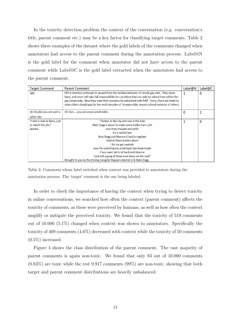
In the toxicity detection problem the context of the conversation (e.g. conversation’s

title, parent comment etc.) may be a key factor for classifying target comments. Table 2

shows three examples of the dataset where the gold labels of the comments changed when

annotators had access to the parent comment during the annotation process. Label@N

is the gold label for the comment when annotator did not have access to the parent

comment while Label@C is the gold label extracted when the annotators had access to

the parent comment.

Table 2: Comments whose label switched when context was provided to annotators during the

annotation process. The ‘target’ comment is the one being labeled.

In order to check the importance of having the context when trying to detect toxicity

in online conversations, we searched how often the context (parent comment) affects the

toxicity of comments, as these were perceived by humans, as well as how often the context

amplify or mitigate the perceived toxicity. We found that the toxicity of 519 comments

out of 10.000 (5.1%) changed when context was shown to annotators. Specifically the

toxicity of 469 comments (4.6%) decreased with context while the toxicity of 50 comments

(0.5%) increased.

Figure 4 shows the class distribution of the parent comment. The vast majority of

parent comments is again non-toxic. We found that only 83 out of 10.000 comments

(0.83%) are toxic while the rest 9.917 comments (99%) are non-toxic, showing that both

target and parent comment distributions are heavily unbalanced.

13

Figure 4: Class Distribution of parent comment.

Figure 5 shows the class percentage of the target comments based on the class of the

parent comment. The percentage of the non-toxic class is almost the same whether the

parent comment is non-toxic or toxic. On the other hand, when the parent is toxic the

percentage of the toxic class is almost 20 times bigger than the percentage of the toxic

class when the parent comment is non-toxic.

Figure 5: Class Percentage of each class based on parent’s class.

2.3 CCTK With Probabilistic Labels

The true nature of the ground truth annotations is not a binary one. Moreover, the score

that is obtained from the annotation is in effect an estimation of the probability that a

comment is toxic or not or unsure. To be more accurate with the real problem’s nature

we created the “CCTK With Probabilistic labels” (or CCTK.v2 in short). In this dataset

instead of having a gold label for each comment we have a gold distribution that consists

14

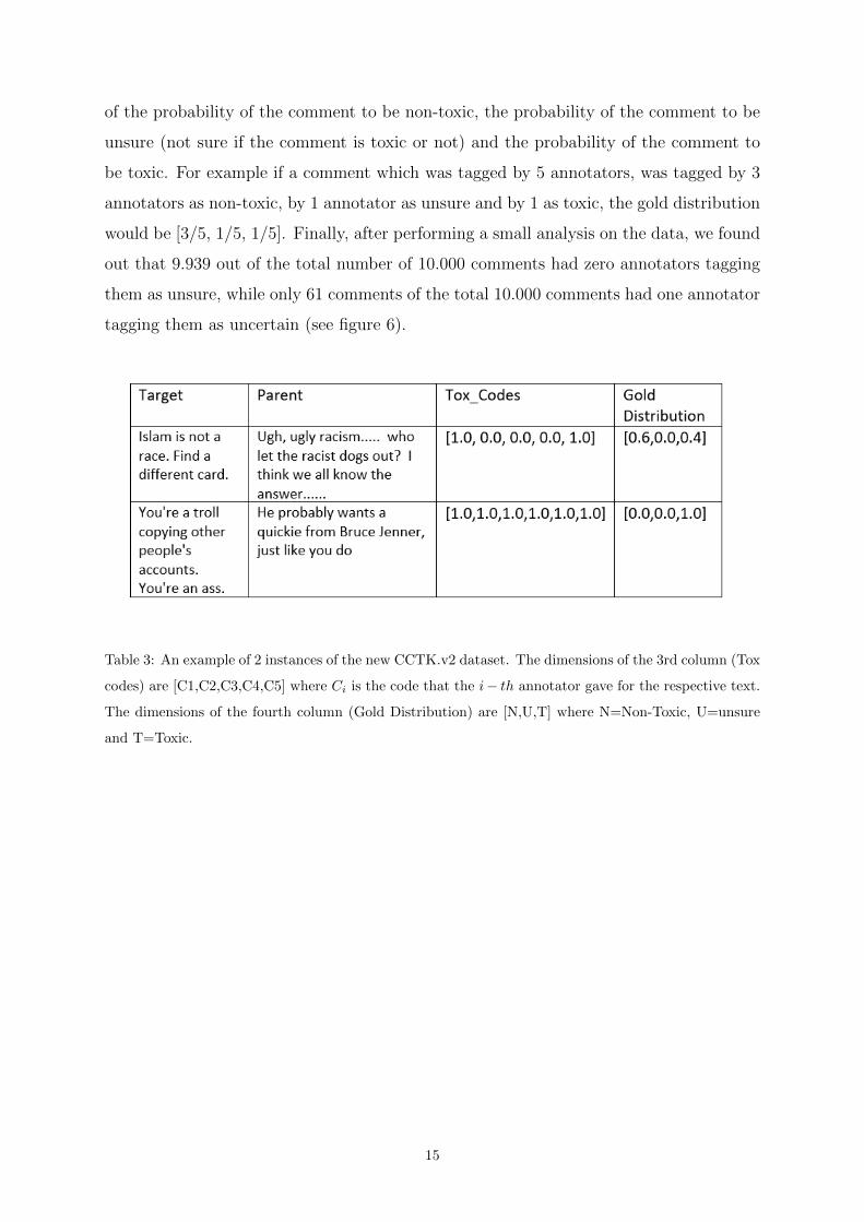
of the probability of the comment to be non-toxic, the probability of the comment to be

unsure (not sure if the comment is toxic or not) and the probability of the comment to

be toxic. For example if a comment which was tagged by 5 annotators, was tagged by 3

annotators as non-toxic, by 1 annotator as unsure and by 1 as toxic, the gold distribution

would be [3/5, 1/5, 1/5]. Finally, after performing a small analysis on the data, we found

out that 9.939 out of the total number of 10.000 comments had zero annotators tagging

them as unsure, while only 61 comments of the total 10.000 comments had one annotator

tagging them as uncertain (see figure 6).

Table 3: An example of 2 instances of the new CCTK.v2 dataset. The dimensions of the 3rd column (Tox

codes) are [C1,C2,C3,C4,C5] where Ci is the code that the i− th annotator gave for the respective text.

The dimensions of the fourth column (Gold Distribution) are [N,U,T] where N=Non-Toxic, U=unsure

and T=Toxic.

15

Figure 6: Distribution of posts based on number of unsure codes.

Figure 6 shows the the distribution of posts based on the number of unsure codes. Only

in 61 comments one annotator said unsure while for the rest 9.939 comments no annotator

tagged the comment as unsure. It seems that annotators voted for one category non-toxic

or toxic even if they were not 100% sure. Consequently we deleted these 61 comments

from the CCTK.v2 dataset because we could not exploit this information properly.

Figure 7: Distribution of posts based on number of non-toxic codes vs Distribution of posts based on

number of toxic codes.

Figure 7 shows the distribution of the posts based on the number of non-toxic codes

and the distribution of the posts based on the number of toxic codes. The diagram on

the left of figure 7 shows that for the non-toxic category, annotators agreed 100% in most

16

of the cases as in 8.163 out of 10.000 comments, all 5 annotators voted for non-toxic.

On the other hand, regarding the toxic category, things are not so simple. The diagram

on the right makes it clear that toxicity detection is not so obvious even for humans.

There was only a single comment, out of the 10.000, which all 5 annotators found toxic.

Moreover, most often it was up to two annotators (out of five) who found the respective

comment toxic.

2.4 Inter-annotator Agreement

Inter-annotator agreement was computed with percentage agreement or Krippendorff’s

alpha, separately on all comments, on all non-toxic comments and on all toxic comments.

Percentage Agreement Our first statistical measure for inter-annotator agreement

is the percentage agreement. It is one intercoder reliability technique that relies on the

proportion of agreement of coded units between two or more independent judges. To cal-

culate pairwise agreement, you calculate the agreement between a pair of coders. Given

only two coders and one observation, your results can only be 100% (they agree) ore 0%

(they disagree). If you are working with multiple coders and multiple cases, then you

calculate the average pairwise agreement among all possible coder pairs across observa-

tions [32]. The general rule of thumb for percent agreement is presented in Neuendorf:

“Coefficients of .90 or greater are nearly always acceptable, .80 or greater is acceptable

in most situations, and .70 may be appropriate in some exploratory studies for some

indices” (Neuendorf 2002, p. 145) [25].

Krippendorff’s Alpha Our second statistical measure for inter-annotator agreement

is the Krippendorff’s alpha measurement. Krippendorff’s alpha ranges between 1 and 0

but can also take negavtive values :

• a =1 indicates perfect aggreement.

• a = 0 indicates perfect disagreement.

• a < 0 when disagreements are systematic and exceed what can be expected by

chance.

Unlike other specialized coefficients, Krippendorff’s alpha is a generalization of several

known reliability indices [21]. It enables researchers to judge a variety of data with the

same reliability standard applying to:

17

• Any number of observers, not just two

• Any metric or level of measurement (nominal, ordinal, interval, ratio, and more)

• Any number of categories, scale values, or measures.

• Complete or missing data

• Large and small sample sizes alike, not requiring a minimum

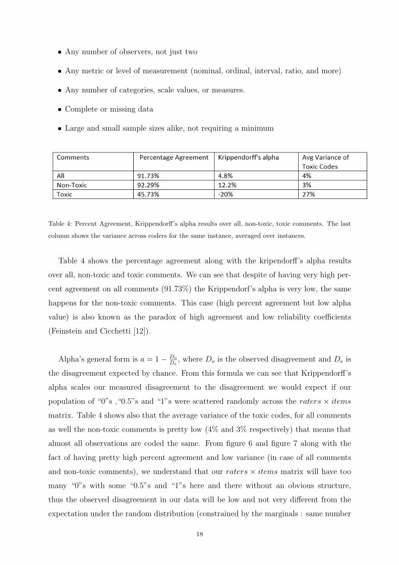
Table 4: Percent Agreement, Krippendorff’s alpha results over all, non-toxic, toxic comments. The last

column shows the variance across coders for the same instance, averaged over instances.

Table 4 shows the percentage agreement along with the kripendorff’s alpha results

over all, non-toxic and toxic comments. We can see that despite of having very high per-

cent agreement on all comments (91.73%) the Krippendorf’s alpha is very low, the same

happens for the non-toxic comments. This case (high percent agreement but low alpha

value) is also known as the paradox of high agreement and low reliability coefficients

(Feinstein and Cicchetti [12]).

Alpha’s general form is a = 1− Do

De, where Do is the observed disagreement and De is

the disagreement expected by chance. From this formula we can see that Krippendorff’s

alpha scales our measured disagreement to the disagreement we would expect if our

population of “0”s ,“0.5”s and “1”s were scattered randomly across the raters × items

matrix. Table 4 shows also that the average variance of the toxic codes, for all comments

as well the non-toxic comments is pretty low (4% and 3% respectively) that means that

almost all observations are coded the same. From figure 6 and figure 7 along with the

fact of having pretty high percent agreement and low variance (in case of all comments

and non-toxic comments), we understand that our raters × items matrix will have too

many “0”s with some “0.5”s and “1”s here and there without an obvious structure,

thus the observed disagreement in our data will be low and not very different from the

expectation under the random distribution (constrained by the marginals : same number

18

of “0”s ,“0.5”s “1”s) which will also be low since the few “0.5”s and “1”s are here and

there. Consequently the fraction Do

Dewill be very close to 1 leading to a very small alpha

value. On the other hand things would have been different if our rating matrix had the

following structure : still an ocean of ”0”s but with the “0.5”s and “1”s concentrated

on a few items separately, then, our percent agreement would be even higher but, more

importantly, our measured number of disagreements (Do) would be significantly smaller

than what would be expected (De) if the “0.5”s and “1”s were scattered randomly across

the matrix. Because of this structure, with the same marginal as above, we would have

a much higher Krippendorff’s alpha.

In the case of toxic comments, table 4 shows that the average variance of the toxic

codes of toxic comments is much larger that the variance of the other two categories.

That means that there is bigger diversity of coded values in toxic comments and that can

be seen in Figure 6 and Figure 7, thus that is the reason we have the smallest percentage

agreement in this category. Because of the high variance, the observed disagreement will

be very high and bigger than the expected disagreement. Because of this the fraction Do

De

will be greater than 1 and the Krippendorff’s alpha will be negative.

So in the case of overall comments low coefficient does not mean invalid data due to

the paradox (high agreement but low alpha) explained above.

The interested reader is referred to [21], for more details on the Krippendroff’s alpha

and the way it is coumputed. For more details on the kappa coefficients paradoxes, the

interested reader is referred to [12].

2.5 A Toy Example

In this section a hypothetical concrete toy example is used, with 5 coders and 5 posts,

showing the raters × items matrix in the two different scenarios (with/without ”struc-

ture”). For the computation of the observed disagreement (Do), the expected disagree-

ment (De) and the Krippendroff’s alpha, the python package Krippendorff PyPI was used

1.1Code can be found here https://github.com/pln-fing-udelar/fast-krippendorff/blob/master/krippendorff/

krippendorff.py.

19

Table 5: A raters×items matrix with 5 coders and 5 posts with some “1”s without any obvious structure.

Table 5 shows the first scenario where we have a raters× items matrix with 5 coders

and 5 posts containing an “ocean” of “0”s with some “1”s here and there without any

structure. Even though the percent agreement and the average variance of the codes

across all instances seems to be high (76%) and low (12%) respectively, Krippendorff’s

alpha is negative (-0.9). The fact that we have high percent agreement and low average

variance means that almost all observations are coded the same which in this case is true.

Because of the three “1”s that are randomly spread in three different posts without any

obvious structure, the observed disagreement in our data will be low and not very different

from the expectation under the random distribution (constrained by the marginals : same

number of “0”s and “1”s) which will also be low since the few “1”s are here and there.

Indeed in this scenario we have, Do = 6, De = 5.5 and Do

De= 1.09. As a result we have a

negative Krippendorff’s alpha value.

Table 6: A raters× items matrix with 5 coders and 5 posts with some “1”s concentrated in one post.

Table 6 shows the second scenario where we have a raters × items matrix with 5

coders and 5 posts containing an “ocean” of “0”s with some “1”s concentrated only in

a few items (here only one post). In this example the percent agreement is even bigger

(88%) as we would expect and the average variance of the codes across all instances is

6%. Because the “1”s are concentrated only in one post, the observed disagreement (Do)

20

will be significantly smaller than what would be expected (De) if the “1”s were scattered

randomly across the matrix. Indeed in this scenario we have, Do = 3, De = 5.5 and

Do

De= 54.54. As a result we have a much bigger Krippendorff’s alpha value (45.45).

21

3 Experiments

3.1 Training Procedure

For the experiments with both the CCTK.v1 and CCTK.v2 datasets, we used 5-fold

Monte Carlo Cross Validation (Qing-Song Xu and Yi-Zeng Liang [42]), where in each

fold we randomly selected (without replacement) 60% of our data to form the training

set, and then we assigned the rest 20% to form the validation set and the rest 20% to

form the test set. Both the validation set and the test set consist of comments obtained

from the CCTK@C.v1 dataset, where the comments were labeled by annotators who had

access to context (parent comment), assuming that those labels are more reliable (the

annotators had a broader view of the discussion). Stratified splits were used to retain the

same distribution over classes in the train, val and test sets.

Figure 8: Demonstration of 5-fold MC Cross Validation.

3.2 Evaluation Metrics

In Order to evaluate our models we used a variety of different classification metrics.

PRECISION Our first classification metric is the precision of the positive class. It is

a measure to evaluate how the model actually performs on predicting the positive class

(here the positive class is the toxic class). It is the fraction of the number of comments

that the model classified as toxic and they actually were (also known as “true positives”),

divided by the number of the total comments that the model classified as toxic.

Precision = True PositivesTrue Positives +False Positives

22

RECALL Our second classification metric is recall (also known as sensitivity). It quan-

tifies the number of positive class predictions made by the model out of all positive

examples in the dataset. It is the fraction of the total amount of relevant instances that

were actually retrieved.

Recall = True PositivesTrue Positives +False Negatives

F1 SCORE Our third classification metric is the F1 score. It is the harmonic mean of

the precision and recall. The highest possible value of F1 is 1, indicating perfect precision

and recall, and the lowest possible value is 0, which occurs when either the precision or

the recall is zero.

F1 = 2 · Precision · RecallPrecision + Recall

ROC AUC Our last classification metric is the ROC area under the curve (AUC) score.

Here we used the total area under the ROC curve (AUC) [1]. This is a standard classifi-

cation metric that gives the performance of a binary classifier averaged over all possible

trade-offs between true positive predictions and false positive predictions. The ROC

curve is created by plotting the true positive rate (TPR) against the false positive rate

(FPR) at various threshold settings. The true-positive rate is also known as sensitivity,

recall or probability of detection. The false-positive rate is also known as probability of

false alarm and can be calculated as 1 - specificity, where specificity is the recall of the

negative class..

23

True Positive Rate(TPR) = TPTP +FN

False Positive Rate(FPR) = FPFP +TN

Figure 9: Illustration of the ’ROC’ curve. (Source https://developers.google.com/

machine-learning/crash-course/classification/roc-and-auc).

The area under the ROC Curve (“AUC”) measures the entire two-dimensional area

underneath the entire ROC curve from (0,0) to (1,1) (see figure 10). It provides an

aggregate measure of performance across all possible classification thresholds. One way

of interpreting AUC is as the probability that the model ranks a random positive example

more highly than a random negative example [11].

24

Figure 10: Illustration of the ’AUC’ (Area Under the ROC Curve). (Source https://developers.

google.com/machine-learning/crash-course/classification/roc-and-auc).

Moreover, we used this metric to make a final choice among all models, we considered

the best model as the one with the highest AUC score.

3.3 Experiments on CCTK with Binary Labels

3.3.1 Context-Unaware Models

BILSTM Our first context-unaware model is a bidirectional LSTM (Hochreiter and

Schmidhuber, 1997 [16]). We concatenate the outputs of the last hidden states (from the

two directions) of the BILSTM, and we add on top of that a feed-forward neural network

(FFNN), consisting of a hidden dense layer with 128 neurons and tanh activations. Finally

we add a dense layer leading to a single output neuron with a sigmoid activation that

produces the toxicity probability. To counter bias against the majority (non-toxic) class,

we fix the bias term of the single output neuron to log TN

, where T and N are the numbers

of toxic and non-toxic training comments, respectively. We could add more complexity

to this model of course, for example by stacking more BILSTM layers, but we use it more

as baseline model.

25

Figure 11: Architecture of BILSTM Model.

BERT Our second context-unaware classifier is BERT (Bidirectional Encoder Rep-

resentations from Transformers) Devlin et al. [8]. BERT is a pre-trained model trained

on a large corpus of text documents from Wikipedia and uses Transformers [36]. Using

transfer learning along with this architecture, BERT is able to get state-of-the-art results

on many NLP tasks. We fine-tuned BERT on the training subset of each experiment, with

a task-specific classifier on top, fed with BERT’s top-level embedding of the [CLS] token.

We used BERT-BASE pre-trained on cased data, with 12 layers and 768 hidden units and

110M parameters in total. We only unfreezed the top three layers during fine-tuning, with

a small learning rate (2e-05) to avoid catastrophic forgetting. The task-specific classifier

is the same FFNN as in the BILSTM classifier.

26

Figure 12: The Transformer – Model Architecture. Taken from Vaswani et al. [36].

27

Figure 13: BERT – Model Architecture.

PERSPECTIVE Our next context-unaware model is PERSPECTIVE. It is a CNN-based

model created by Jigsaw and Google’s Counter Abuse Technology team for toxicity detec-

tion. It is trained on millions of user comments from online publishers and conversations.

It is publicly available through the PERSPECTIVE API 2.

3.3.2 Context-Aware Models

CA-SEP-BERT Our first context-aware model is CA-SEP-BERT. It is a BERT-based model

with a simple context-aware mechanism added and the same task-specific classifier as2https://www.perspectiveapi.com/

28

in the simple BERT model. This model does not use a separate encoder for the parent

comment (context), however it concatenates the text of the parent and target comments,

separated by BERT’s [SEP] token, as in BERT’s next sentence prediction pre-training

task (see Fig. 14). We used the training subset to fine-tune the model.

Figure 14: CA-SEP-BERT – Model Architecture.

CA-CONC-BERT Our second context-aware model is CA-CONC-BERT. It is exactly the

same BERT-based model with our first context-unaware BERT. This time we added a

naive context-awareness mechanism to the model by concatenating the text of the parent

comment and the target comment during train time as well as during test time.

CA-CONC-PERSPECTIVE Our last context-aware model is CA-CONC-PERSPECTIVE. It

is exactly the same model with PERSPECTIVE. We use the same context-awareness mech-

anism as we did for CA-CONC-BERT, this time by concatenating the text of the target

comment and the parent comment only during test time.

3.3.3 Experimental Results

All models were trained for a maximum of 10 epochs with a batch size of 128 training

examples. We used Binary Cross Entropy loss to train our models. We also used adam

29

optimizer (Kingma and Ba [20]) with default parameters (learning rate 1e-03) for the

BiLSTM model and for the Bert-based models we used a learning rate of (2e-05) to avoid

catastrophic forgetting.

For the vector representations of the tokens 3 we used new token embeddings of size

100. For the BiLSTM model we used a max sequence length of 512 tokens. To deal with

sequences that had more than 512 tokens we truncated them to just have 512. To deal

with sequences that had less than 512 tokens, we used zero padding. We did the same

for the Bert-based models but this time using a max sequence length of 128 tokens.

During train time, we performed Early stopping (Prechel [33]) with patience 3 epochs

monitoring the ROC AUC on the validation data as we wanted to optimize models based

on the ROC AUC score.

Each model was trained twice, at first using gold labels obtained when context was not

provided to the annotators (@N models) and secondly using gold labels obtained with

context (@C models) but for the evaluation and the validation of the models we only

used gold labels that were obtained with context as we mentioned in section 3.1. In order

to evaluate our models we used the test set.

From this set we extracted 2 more gold test subsets, the “Label Switched Comments”

and the “Label Not Switched Comments”. The first one consists of all the target com-

ments (in Test set) whose gold label changed after annotators showed the parent comment

while the second one consists of all the target comments (in Test set) whose gold label

did not change with context. This way we could focus on how does our models perform

on classifying comments where context matters and how on comments that context does

not matter.3A token here can be a word (BiLSTM) or a sub-word (Bert).

30

Table 7: Experimental results (Precision, Recall, F1, ROC AUC) using the CCTK.v1 dataset. Label

Switched Comments are the comments whose gold label changed when context was provided to annota-

tors. Label Not Switched Comments are the comments whose gold label did not change when context

was provided to annotators. @N models were trained with gold labels obtained without context. @C

models were trained with gold labels obtained with context.

Table 7 shows the experimental results using the “CCTK With Binary Labels” dataset.

We report the Precision, Recall, F1 and ROC AUC score (averaged, using 5-fold Monte

Carlo Cross Validation [42]). We gave more attention to the ROC AUC score since it

is better from the remaining measures because it is a classification-threshold-invariant

metric since it measures the quality of the model’s predictions irrespective of what clas-

sification threshold is chosen. The default classification threshold (0.5) was used for the

rest of the measures.

A first observation is that training with gold labels obtained while context was not

shown to the annotators (@N models) lead always to better results (ROC AUC) when

evaluating on the “Label Not Switched Comments” gold subset whether the models are

context-aware or not. Instead training with gold labels obtained with context (@C mod-

els) lead always to better results (ROC AUC) when evaluating on the “Label Switched

Comments” gold subset. Consequently @N models perform always better at the whole

test set (all comments) since the label-switching comments are significantly fewer than

the label not-switched comments.

31

A second observation is that in overall performance (when evaluating on the whole

test set) the 2 best models based on the ROC AUC metric are the Perspective model and

the Bert model, scoring 91.1% and 93.6% respectively. This is not surprising, since the

Perspective model was trained on much larger toxicity datasets than the other systems

and the Bert model was also pre-trained on even larger corpora.

A more interesting observation is that context-aware models always perform better

than the respective context-unaware models when they are getting evaluated at the “La-

bel Switched Comments” gold subset where context matters. For example CA-SEP-

BERT@C and CA-CONC-BERT@C both perform better than BERT@C with 43.6%,

45.4% and 40% ROC AUC scores respectively. This also applies to the Perspective

model where Perspective and CA-CONC-Perspective are scoring 27.2% and 59.4% ROC

AUC scores respectively.

Finally, what is more surprising is that the BILSTM@C model although does not have

any context mechanism, it has the second best ROC AUC score (54.6%) following the

Perspective-CA-CONC model that takes the first place when evaluating on the “Label

Switched Comments” gold subset. BiLSTM surpasses by 10-15% all the BERT-based

models with or without context mechanism, proving that it is a powerful and useful

baseline model.

We conclude that training with gold labels obtained while context was not provided

to the annotators help models to perform better at the “Label Not Switched Comments”

gold subset whether the model is context-aware or not, while training with gold labels

obtained with context help models to perform better at “Label Switched Comments” gold

subset where context matters. Moreover we conclude that making the models context-

aware even with a very naive context mechanism (e.g. by concatenating the target with

the parent text during training and testing time) increases slightly the performance, when

the models are getting evaluated on comments that context matters (“Label Switched

Comments” gold subset).

3.4 Experiments on CCTK with Probabilistic Labels

As already mentioned in section 2.3 the true nature of the ground truth annotations not

being a binary one made us develop the “CCTK with Probabilistic Labels” (or CCTK.v2

in short) dataset, where instead of having binary gold labels, we have a gold distribution

(gold probabilistic labels) for each comment (see section 2.3 for more details on the

32

creation of this dataset). To be more accurate with the true nature of the ground truth

annotations, we wanted to train deep learning models which take the text from the target

comment as input and instead of giving as output the class of the comment, they would

give as output 3 different probabilities that sum up to 1. These would be, the probability

of the comment to be non-toxic, the probability of the comment to be unsure (not sure

if the comment is toxic or not) and the probability of the comment to be toxic. But

after performing a small analysis on the data, we found out that 9.939 out of the total

number of 10.000 comments had 0 annotators tagging them as unsure, while only 61

comments of the total 10.000 comments had 1 annotator tagging them as unsure (see

figure 6). Consequently we deleted these 61 comments from the dataset and we changed

the architectures of our models. Instead of having 3 outputs we only have 1 output, the

toxicity of the comment.

For our Experiments with CCTK.v2 we used the same models as in our experiments

with CCTK.v1 with some small changes. Because we now have a regression problem we

performed 5 experiments trying to find the one that works better. To train our models we

used the Mean Squared Error loss as we were trying to solve a regression problem. Since

the problem has a probabilistic nature, we also used Binary Cross Entropy in some of

the experiments, with the gold label instead of being binary (1 or 0), being the real toxic

probability extracted from the annotators (for example if the toxic codes of a comment

were [0,0,0,1,1] the gold toxic probability would be 2/5).

We performed the following experiments :

1. MSE loss, unconstrained predicted score.

2. MSE loss, predicted score constrained to interval [0,1] by 1 ReLU with max value = 1.

3. BCE loss, predicted score constrained to interval [0, 1] by 1 ReLU with max value = 1.

4. MSE loss, predicted score constrained to interval [0, 1] by sigmoid.

5. BCE loss, predicted score constrained to interval [0, 1] by sigmoid.

In all 5 experiments we used exactly the same hyper parameters as those used in

the experiments with the CCTK.v1 dataset. Specifically, all models were trained for a

maximum of 10 epochs with a batch size of 128 training examples. We also used adam

optimizer (Kingma and Ba, [20]) with default parameters (learning rate 1e-03) for the

BiLSTM model and for the Bert-based models we used a learning rate of (2e-05) to avoid

catastrophic forgetting.

33

For the vector representations of the tokens 4 we used new token embeddings of size

100. For the BiLSTM model we used a max sequence length of 512 tokens. To deal with

sequences that had more than 512 tokens we truncated them to just have 512. To deal

with sequences that had less than 512 tokens, we used zero padding. We did the same

for the Bert-based models but this time using a max sequence length of 128 tokens.

During train time, we performed Early stopping [33] with patience 3 epochs monitoring

the MSE on the validation data.

Finally, in order to evaluate our models we used the same evaluation metrics as those

used for the CCTK.v1 experiments. We used the default classification threshold (0.5).

3.4.1 Experimental results

We chose to report only the experimental results of the last experiment (“BCE loss,

predicted score constrained to interval [0, 1] by sigmoid”) since the results of the

other 4 experiments did not differ that much and because this experiment had the better

results among all the others.

In this experiment we trained our models using the BCE (Binary Cross Entropy) loss.

Moreover we add a sigmoid activation function on the output layer of the FFNN (Feed

Forward Neural Network) that produces the toxic probability to constrain the output to

the [0, 1] interval. To counter bias against the majority (non-toxic) class, we used the

same trick as before (see section 3.3), fixing the bias term of the single output neuron

to log TN

, where T and N are the numbers of toxic and non-toxic training comments,

respectively. This time we applied this trick only to the Bert-based models because we

found that the BILSTM model performs better without it.

For the experiments with the “CCTK With Probabilistic Labels” dataset we only

have models that were trained with gold probabilistic labels (for each comment) obtained

while context (parent comment) was shown to the annotators (models @C), since in this

dataset we do not have the toxic codes that the annotators gave when they were not

provided with context.

From the test set we extracted 2 more gold test subsets, the “Label Switched Com-

ments” and the “Label Not Switched Comments” as we did for the experiments with

the CCTK.v1 dataset. The first one contains comments where the gold binary label (as

extracted for the CCTK.v1 experiments) changed when annotators had access to context

4A token here can be a word (BiLSTM) or a sub-word (Bert).

34

while the second one contains comments whose gold binary label did not change with

context.

Table 8: Experimental results (Precision, Recall, F1, ROC AUC) using the CCTK.v2 dataset. Label

switched Comments are the comments whose gold label changed when context was provided to annota-

tors. Label Not Switched Comments are the comments whose gold label did not change when context

was provided to annotators. @C models were trained with gold distribution obtained with context.

Table 8 shows the experimental results from the “BCE loss, predicted score con-

strained to interval [0, 1] by sigmoid” experiment. We evaluate our models as

classifiers and not as regressors by binarizing the gold labels of the test set using the

default classification threshold (0.5). We report the Precision, Recall, F1 and ROC

AUC score (averaged, using 5-fold Monte Carlo Cross Validation [42]) as we did in the

CCTK.v1 experiments. As in the CCTK.v1 experiments, we gave more attention to the

ROC AUC score since it is better from the remaining measures because it does not use

a classification threshold.

A first observation is that the Perspective model and the Bert-based models outper-

form the BILSTM model on the ROC AUC score when evaluating on the whole test

set (All comments) but this is not surprising because as we said earlier the Perspective

model was trained on much larger toxicity datasets than the other systems and the Bert

model was also pre-trained on even larger corpora. A more significant observation is that

35

when evaluating on the “Label Switched Comments” test subset where context matters,

the model with the worst performance is the Perspective model with 30.8% ROC AUC

score showing that Perspective has a potential weakness in addressing comments where

context matters. Another observation is that the context-aware models perform slightly

better on the “Label Switched Comments” gold test subset than the models without any

context mechanism but that is not the case when evaluating on the “Label Not Switched

Comments”. In this case the context-mechanism slightly decreases the performance of

the models.

3.5 Comparison Of The Two Datasets

For the experiments with the “CCTK With Binary Labels” (CCTK.v1) dataset we sim-

plified the problem by binarizing the ground truth annotations. But the true nature

of the ground truth annotations is not binary, because the annotators are asked to tag

each comment as non-toxic, unsure or toxic and therefore they compound a distribution

(of 3 categories) for each comment. To face this problem, we experiment with both the

CCTK.v1 and CCTK.v2 datasets (CCTK With Probabilistic Labels).

We compared these 2 datasets based only on the ROC AUC metric because it is

a classification-threshold-invariant metric since it measures the quality of the model’s

predictions irrespective of what classification threshold is chosen.

We compared only the models that were trained with gold binary labels (in case

of the CCTK.v1 experiments) and gold probabilistic labels (in case of the CCTK.v2

experiments) obtained when context (parent comment) was shown to the annotators

(@C models). We could not compare the models that were trained with gold binary

labels and gold probabilistic labels obtained without context (@N models) because we do

not have the toxic codes that annotators gave when context was not shown to them.

36

Table 9: Comparison of the Experimental results (ROC AUC) of CCTK.v1 and CCTK.v2 datasets.

Label switched Comments are the comments whose gold label changed when context was provided to

annotators. Label Not Switched Comments are the comments whose gold label did not changed when

context was provided to annotators. @C models were trained with gold distribution obtained with

context.

Table 9 shows the ROC AUC results from the experiment when using the CCTK.v1

dataset and the ROC AUC results from the“BCE loss, predicted score constrained

to interval [0, 1] by sigmoid” experiment when using the CCTK.v2 dataset.

Even though we would expect the CCTK.v1 results to be better in all categories

because of the binarization that was performed on the ground truth annotations that

simplifies the problem, that is not the case. We observed that all the models except the

CA-CONC-BERT model that were trained with probabilistic labels (CCTK.v2 ) perform

better than the models that were trained with binary labels when evaluating at the whole

test set (All Comments). The same seems to be true when evaluating on the “Label Not

Switched Comments” gold test subset where context does not matter.

When evaluating on the “Label Switched Comments” gold test subset where context

matters, the models that were trained with binary labels as well as the models trained with

probabilistic labels have very low performance. Moreover in both experiments (CCTK.v1

and CCTK.v2) context-aware models seem to increase slightly the performance of the

models, showing that even adding naive context aware mechanisms to models can improve

their performance when trying to detect toxicity in comments that context matters.

Another important observation is that in both experiments when evaluating on the

37

“Label Switched Comments” gold test subset, the BILSTM model outperforms the Bert-

based models (with or without context aware mechanism) and the Perspective model

(with or without context aware mechanism) in case of the CCTK.v2 dataset, showing

how powerful and useful baseline model is.

Finally, we observed that in the “Label Switched Comments” gold test subset the

context aware version of the Perspective model (CA-CONC-Perspective) when predicting

gold binary labels outperforms the CA-CONC-Perspective model when trying to predict

probabilistic labels.

38

4 Conclusions and future work

In this thesis we investigated the role of context in detecting toxic online comments. We

created two alternate versions (CCTK.v1 and CCTK.v2) of an unreleased (yet) dataset,

which was developed by others, for investigating how training with gold binary labels as

well as training with gold probabilistic labels affects the performance of the models.

It was shown that context does have an effect on toxicity annotation, but this effect

is seen in only a narrow slice (5.1%) of the first dataset. We also found that training

toxicity classifiers with gold labels obtained without context increases their performance

when evaluating on comments where context does not matter; but training with gold

labels obtained when context was shown to the annotators improves their performance

when evaluating on comments where context matters.

Moreover we found that when evaluating on the “Label Switched Comments” gold

test subset where context matters the performance of the models decreases significantly.

In addition to that we found that by adding an even naive context aware-mechanism

to models (e.g. target’s text and parent’s text concatenation) can improve slightly the

performance of the classifiers. The two above findings may be the proof that if we create

better context-aware models and use better datasets (not so heavily unbalanced) and

with more context-sensitive comments, we could improve by a lot the performance of our

classifiers in cases where the context matters.

A limitation of our work is that we considered only a small contextual window, con-

sisting of only the previous comment and the discussion title. As Pavlopoulos et al. [31]

proposed, it would be interesting to investigate in future work ways to improve the an-

notation quality when more comments in the discussion thread are provided, and also if

our findings hold when broader context is considered (e.g., all previous comments in the

thread, or the topic of the thread as represented by a topic model). Another limitation

of our work is that we used randomly sampled comments. As Pavlopoulos et al. [31]

pointed out, the effect of context may be more significant in conversations about partic-

ular topics, or for particular conversational tones (e.g. sarcasm), or when they reference

communities that are frequently the target of online abuse.

As regards our models and the context’s effect analysis, a limitation of our work is

that we used very simple and naive context-aware mechanisms. It would be challenging

to investigate in future work more complex context-aware models (e.g. use a Bert model

to encode each parent and target comment and then train a MLP which concatenates

39

the two [CLS] embeddings).

Also another limitation is that in the experiments with the CCTK.v2 dataset we

trained our models using early stopping and monitoring (optimizing) the MSE on the

validation data. This is problematic because the dataset is heavily unbalanced and con-

sequently MSE is very easy to be “hacked” just like the accuracy metric can be “hacked”

in a classification problem with a heavily unbalanced dataset. It would be interesting in

future work to create custom metrics that are not affected by the major class.

Finally we leave for future work the classification threshold tuning so we can perform

an even better comparison of the performances of the models. We also leave for future

work the evaluation of our models with the PR AUC metric, the PR gain AUC metric

and the MCC metric, since these metrics are more suitable metrics than the ROC AUC

for heavily unbalanced datasets ([7], [13], [46]).

40

References

[1] A. P. Bradley. “The use of area under the ROC curve in the evaluation of machine learning

algorithms”. In: Pattern Recognition 30.7 (1997), pp. 1145–1159.

[2] Tuhin Chakrabarty, Kilol Gupta, and Smaranda Muresan. “Pay “Attention” to your Context

when Classifying Abusive Language”. In: Proceedings of the Third Workshop on Abusive Language

Online. Florence, Italy: Association for Computational Linguistics, Aug. 2019, pp. 70–79. doi:

10.18653/v1/W19-3508. url: https://www.aclweb.org/anthology/W19-3508.

[3] Patricia Chiril, Veronique Moriceau, Farah Benamara, Alda Mari, Gloria Origgi, and Marlene

Coulomb-Gully. “An Annotated Corpus for Sexism Detection in French Tweets”. English. In:

Proceedings of The 12th Language Resources and Evaluation Conference. Marseille, France: Euro-

pean Language Resources Association, May 2020, pp. 1397–1403. isbn: 979-10-95546-34-4. url:

https://www.aclweb.org/anthology/2020.lrec-1.175.

[4] Junyoung Chung, Caglar Gulcehre, KyungHyun Cho, and Yoshua Bengio. Empirical Evaluation of

Gated Recurrent Neural Networks on Sequence Modeling. 2014. arXiv: 1412.3555 [cs.NE].

[5] Thomas Davidson, Debasmita Bhattacharya, and Ingmar Weber. Racial Bias in Hate Speech and

Abusive Language Detection Datasets. 2019. arXiv: 1905.12516 [cs.CL].

[6] Thomas Davidson, Dana Warmsley, Michael Macy, and Ingmar Weber. Automated Hate Speech

Detection and the Problem of Offensive Language. 2017. arXiv: 1703.04009 [cs.CL].

[7] Jesse Davis and Mark Goadrich. “The Relationship between Precision-Recall and ROC Curves”.

In: Proceedings of the 23rd International Conference on Machine Learning. ICML ’06. Pittsburgh,

Pennsylvania, USA: Association for Computing Machinery, 2006, pp. 233–240. isbn: 1595933832.

doi: 10.1145/1143844.1143874. url: https://doi.org/10.1145/1143844.1143874.

[8] Jacob Devlin, Ming-Wei Chang, Kenton Lee, and Kristina Toutanova. BERT: Pre-training of Deep

Bidirectional Transformers for Language Understanding. 2018. arXiv: 1810.04805 [cs.CL].

[9] Nemanja Djuric, Jing Zhou, Robin Morris, Mihajlo Grbovic, Vladan Radosavljevic, and Narayan

Bhamidipati. “Hate Speech Detection with Comment Embeddings”. In: Proceedings of the 24th

International Conference on World Wide Web. WWW ’15 Companion. Florence, Italy: Association

for Computing Machinery, 2015, pp. 29–30. isbn: 9781450334730. doi: 10.1145/2740908.2742760.

url: https://doi.org/10.1145/2740908.2742760.

[10] Mai ElSherief, Vivek Kulkarni, Dana Nguyen, William Yang Wang, and Elizabeth Belding. Hate

Lingo: A Target-based Linguistic Analysis of Hate Speech in Social Media. 2018. arXiv: 1804.04257

[cs.CL].

[11] T. Fawcett. “An introduction to ROC analysis”. In: Pattern Recognition Letters 27 (2006), pp. 861–

874.

41

[12] Alvan R. Feinstein and Domenic V. Cicchetti. “High agreement but low Kappa: I. the problems

of two paradoxes”. In: Journal of Clinical Epidemiology 43.6 (1990), pp. 543–549. issn: 0895-4356.

doi: https://doi.org/10.1016/0895-4356(90)90158-L. url: http://www.sciencedirect.

com/science/article/pii/089543569090158L.

[13] Peter Flach and Meelis Kull. “Precision-Recall-Gain Curves: PR Analysis Done Right”. In: Ad-

vances in Neural Information Processing Systems 28. Ed. by C. Cortes, N. D. Lawrence, D. D. Lee,

M. Sugiyama, and R. Garnett. Curran Associates, Inc., 2015, pp. 838–846. url: http://papers.

nips.cc/paper/5867-precision-recall-gain-curves-pr-analysis-done-right.pdf.

[14] Bjorn Gamback and Utpal Kumar Sikdar. “Using Convolutional Neural Networks to Classify Hate-

Speech”. In: Proceedings of the First Workshop on Abusive Language Online. Vancouver, BC,

Canada: Association for Computational Linguistics, Aug. 2017, pp. 85–90. doi: 10.18653/v1/W17-

3013. url: https://www.aclweb.org/anthology/W17-3013.

[15] Lei Gao and Ruihong Huang. Detecting Online Hate Speech Using Context Aware Models. 2017.

arXiv: 1710.07395 [cs.CL].

[16] Sepp Hochreiter and Jurgen Schmidhuber. “Long Short-Term Memory”. In: Neural Computation

9.8 (1997), pp. 1735–1780. doi: 10.1162/neco.1997.9.8.1735. eprint: https://doi.org/10.

1162/neco.1997.9.8.1735. url: https://doi.org/10.1162/neco.1997.9.8.1735.

[17] I.Koutsikakis. “Toxicity Detection in User Generated Content”. MSc thesis (in English), Depart-

ment of Informatics, Athens University of Economics and Business. 2018.

[18] Muhammad Okky Ibrohim and Indra Budi. “A Dataset and Preliminaries Study for Abusive Lan-

guage Detection in Indonesian Social Media”. In: Procedia Computer Science 135 (2018). The 3rd

International Conference on Computer Science and Computational Intelligence (ICCSCI 2018) :

Empowering Smart Technology in Digital Era for a Better Life, pp. 222–229. issn: 1877-0509. doi:

https://doi.org/10.1016/j.procs.2018.08.169. url: http://www.sciencedirect.com/

science/article/pii/S1877050918314583.

[19] Yoon Kim. Convolutional Neural Networks for Sentence Classification. 2014. arXiv: 1408.5882

[cs.CL].

[20] Diederik P. Kingma and Jimmy Ba. Adam: A Method for Stochastic Optimization. 2014. arXiv:

1412.6980 [cs.LG].

[21] K. Krippendorff. “Computing Krippendorff’s Alpha-Reliability.” In: 2011. url: https://repository.

upenn.edu/asc_papers/43/.

[22] Siwei Lai, Liheng Xu, Kang Liu, and Jun Zhao. “Recurrent Convolutional Neural Networks for Text

Classification”. In: Proceedings of the Twenty-Ninth AAAI Conference on Artificial Intelligence.

AAAI’15. Austin, Texas: AAAI Press, 2015, pp. 2267–2273. isbn: 0262511290.

[23] Shervin Malmasi and Marcos Zampieri. Detecting Hate Speech in Social Media. 2017. arXiv: 1712.

06427 [cs.CL].

42

[24] Hamdy Mubarak, Kareem Darwish, and Walid Magdy. “Abusive Language Detection on Arabic

Social Media”. In: Proceedings of the First Workshop on Abusive Language Online. Vancouver, BC,

Canada: Association for Computational Linguistics, Aug. 2017, pp. 52–56. doi: 10.18653/v1/W17-

3008. url: https://www.aclweb.org/anthology/W17-3008.

[25] Kimberly A. Neuendorf. The Content Analysis Guidebook. SAGE Publications, Inc, 2002.

[26] Chikashi Nobata, Joel Tetreault, Achint Thomas, Yashar Mehdad, and Yi Chang. “Abusive Lan-

guage Detection in Online User Content”. In: Proceedings of the 25th International Conference on

World Wide Web. WWW ’16. Montreal, Quebec, Canada: International World Wide Web Con-

ferences Steering Committee, 2016, pp. 145–153. isbn: 9781450341431. doi: 10.1145/2872427.

2883062. url: https://doi.org/10.1145/2872427.2883062.

[27] Ji Ho Park and Pascale Fung. One-step and Two-step Classification for Abusive Language Detection

on Twitter. 2017. arXiv: 1706.01206 [cs.CL].

[28] John Pavlopoulos, Prodromos Malakasiotis, and Ion Androutsopoulos. Deep Learning for User

Comment Moderation. 2017. arXiv: 1705.09993 [cs.CL].

[29] John Pavlopoulos, Prodromos Malakasiotis, and Ion Androutsopoulos. “Deeper Attention to Abu-

sive User Content Moderation”. In: Proceedings of the 2017 Conference on Empirical Methods in

Natural Language Processing. Copenhagen, Denmark: Association for Computational Linguistics,

Sept. 2017, pp. 1125–1135. doi: 10.18653/v1/D17- 1117. url: https://www.aclweb.org/

anthology/D17-1117.

[30] John Pavlopoulos, Prodromos Malakasiotis, Juli Bakagianni, and Ion Androutsopoulos. Improved

Abusive Comment Moderation with User Embeddings. 2017. arXiv: 1708.03699 [cs.CL].

[31] John Pavlopoulos, Jeffrey Sorensen, Lucas Dixon, Nithum Thain, and Ion Androutsopoulos. Tox-

icity Detection: Does Context Really Matter? 2020. arXiv: 2006.00998 [cs.CL].

[32] “Picking the Best Intercoder Reliability Statistic for Your Digital Activism Content Analysis”. In:

2015.

[33] L. Prechelt. “Early Stopping-But When?” In: Neural Networks: Tricks of the Trade. 1996.

[34] Santhosh Rajamanickam, Pushkar Mishra, Helen Yannakoudakis, and Ekaterina Shutova. Joint

Modelling of Emotion and Abusive Language Detection. 2020. arXiv: 2005.14028 [cs.CL].

[35] Bjorn Ross, Michael Rist, Guillermo Carbonell, Benjamin Cabrera, Nils Kurowsky, and Michael

Wojatzki. Measuring the Reliability of Hate Speech Annotations: The Case of the European Refugee

Crisis. 2017. arXiv: 1701.08118 [cs.CL].

[36] Ashish Vaswani, Noam Shazeer, Niki Parmar, Jakob Uszkoreit, Llion Jones, Aidan N Gomez,

Lukasz Kaiser, and Illia Polosukhin. “Attention is All you Need”. In: Advances in Neural In-

formation Processing Systems 30. Ed. by I. Guyon, U. V. Luxburg, S. Bengio, H. Wallach, R.

Fergus, S. Vishwanathan, and R. Garnett. Curran Associates, Inc., 2017, pp. 5998–6008. url:

http://papers.nips.cc/paper/7181-attention-is-all-you-need.pdf.

43

[37] Zeerak Waseem. “Are You a Racist or Am I Seeing Things? Annotator Influence on Hate Speech

Detection on Twitter”. In: Proceedings of the First Workshop on NLP and Computational Social

Science. Austin, Texas: Association for Computational Linguistics, Nov. 2016, pp. 138–142. doi:

10.18653/v1/W16-5618. url: https://www.aclweb.org/anthology/W16-5618.

[38] Zeerak Waseem, Thomas Davidson, Dana Warmsley, and Ingmar Weber. Understanding Abuse: A

Typology of Abusive Language Detection Subtasks. 2017. arXiv: 1705.09899 [cs.CL].

[39] Zeerak Waseem and Dirk Hovy. “Hateful Symbols or Hateful People? Predictive Features for Hate

Speech Detection on Twitter”. In: Proceedings of the NAACL Student Research Workshop. San

Diego, California: Association for Computational Linguistics, June 2016, pp. 88–93. doi: 10.18653/

v1/N16-2013. url: https://www.aclweb.org/anthology/N16-2013.

[40] Michael Wiegand, Melanie Siegel, and Josef Ruppenhofer. “Overview of the GermEval 2018 Shared

Task on the Identification of Offensive Language”. In: Sept. 2018.

[41] Ellery Wulczyn, Nithum Thain, and Lucas Dixon. “Ex Machina: Personal Attacks Seen at Scale”.

In: Proceedings of the 26th International Conference on World Wide Web. WWW ’17. Perth,

Australia: International World Wide Web Conferences Steering Committee, 2017, pp. 1391–1399.

isbn: 9781450349130. doi: 10.1145/3038912.3052591. url: https://doi.org/10.1145/

3038912.3052591.

[42] Qing-Song Xu and Yi-Zeng Liang. “Monte Carlo cross validation”. In: Chemometrics and Intelligent

Laboratory Systems 56.1 (2001), pp. 1–11. issn: 0169-7439. doi: https://doi.org/10.1016/

S0169- 7439(00)00122- 2. url: http://www.sciencedirect.com/science/article/pii/

S0169743900001222.

[43] Zichao Yang, Diyi Yang, Chris Dyer, Xiaodong He, Alex Smola, and Eduard Hovy. “Hierarchical

Attention Networks for Document Classification”. In: Proceedings of the 2016 Conference of the

North American Chapter of the Association for Computational Linguistics: Human Language Tech-

nologies. San Diego, California: Association for Computational Linguistics, June 2016, pp. 1480–

1489. doi: 10.18653/v1/N16-1174. url: https://www.aclweb.org/anthology/N16-1174.

[44] Marcos Zampieri, Shervin Malmasi, Preslav Nakov, Sara Rosenthal, Noura Farra, and Ritesh Ku-

mar. Predicting the Type and Target of Offensive Posts in Social Media. 2019. arXiv: 1902.09666

[cs.CL].

[45] Ziqi Zhang, David Robinson, and Jonathan Tepper. “Detecting Hate Speech on Twitter Using a

Convolution-GRU Based Deep Neural Network”. In: The Semantic Web. Ed. by Aldo Gangemi,

Roberto Navigli, Maria-Esther Vidal, Pascal Hitzler, Raphael Troncy, Laura Hollink, Anna Tordai,

and Mehwish Alam. Cham: Springer International Publishing, 2018, pp. 745–760. isbn: 978-3-319-

93417-4.

[46] Qiuming Zhu. “On the performance of Matthews correlation coefficient (MCC) for imbalanced

dataset”. In: Pattern Recognition Letters 136 (2020), pp. 71–80. issn: 0167-8655. doi: https:

44

//doi.org/10.1016/j.patrec.2020.03.030. url: http://www.sciencedirect.com/science/

article/pii/S016786552030115X.

45