Department of Energy Technology - Pontoppidanstræde 101 ...
153
Department of Energy Technology - Pontoppidanstræde 101 Aalborg University, Denmark Control of Grid Connected PV Systems with Grid Support Functions Conducted by group PED4 - 1043 -Autumn/ Spring Semester, 2011-2012- IED IED IED IED IED IEC 61850 Smart Grid Control Unit
Transcript of Department of Energy Technology - Pontoppidanstræde 101 ...

Department of Energy Technology - Pontoppidanstræde 101
Aalborg University, Denmark
Control of Grid Connected PV
Systems with Grid Support Functions
Conducted by group PED4 - 1043
-Autumn/ Spring Semester, 2011-2012-
IED
IED
IED
IED
IED
IEC 61850
Smart Grid
Control Unit


III
Title: Control of Grid Connected PV Systems with Grid Support Functions
Semester: 9-10th Semester 2011/2012
Semester theme: Master Thesis
Project period: 15/09/2011 – 31/08/2012
ECTS: 50 ECTS
Supervisor: Bogdan Craciun, Tamás Kerekes, Dezső Séra, Remus Teodorescu
Project group: PED4 / 1043
_____________________________________
Vlad Alexandru Muresan
Copies: [5]
Pages, total: [151]
Appendix: [51]
Supplements: [1CD]
By signing this document, each member of the group confirms that all participated in the
project work and thereby that all members are collectively liable for the content of the
report.
SYNOPSIS:
The increased active power generation due to
increased photovoltaic (PV) installations leads to
voltage rise especially in the low voltage networks
(LV) and can exceed the limits imposed by the
grid codes (GCs). Therefore, the PV capacity is
limited and further investments in the network are
needed.
The project goal is to analyze and improve the
voltage regulation methods for grid connected PV
inverters proposed by the new German grid code.
The support strategies based on reactive power
(cosφ(P) and Q(U)) were modeled and simulated
by performing load flow analysis on a typical LV
distribution network.
An optimized voltage regulation method has been
developed which minimizes the reactive power
consumption using coordinated control. The
Ethernet communication IEC 61850 based on
server/ client architecture was used to exchange
information between PVs and master controller. A
laboratory setup has been developed for the
experimental validation of IEC 61850.

IV

V
Preface
This report has been written by the group PED4 1043 during 9th
–10th
semester at the
Department of Energy Technology, Aalborg University. The project has been carried out
between the 15th
of September 2011 – 31st August 2012.
The first 4 chapters have been written by both students from the group PED4 1043, while
the Chapter 5 of the report was written only by the student Vlad Alexandru Muresan. Due to
unexpected circumstances, the student Vlad Alexandru Muresan could not continue the project
work being involved in re-examinations for course modules and therefore the project has been
divided in 2 different parts. The first project version was submitted by the student Elena
Anamaria Man in 31.05.2012 while the second project version is submitted by the student Vlad
Alexandru Muresan in 31.08.2012 with different Chapter 5 (Experimental Work).
Reading Instructions
The main report can be read as an independent piece, from which the appendices derive
including mathematical calculations, simulations and other details in order to make the main
report more understandable. In this project, the chapters are arranged numerically, whereas
appendixes are sorted alphabetically.
Frequently used constants and abbreviations are described in the report nomenclature list,
which can be found after the table of contents. Sources are inserted using the IEEE method, with
a [number], which refers to the bibliography in the back of the report. Additionally, a CD is
included, which features the report and other source files in digital format.
Acknowledgement
First of all I would like to express my gratitude to my colleague and friend Elena
Anamaria Man for her important contribution to this project.
I gratefully appreciate all the support and guidance received during the carried work
from my supervisors Remus Teodorescu, Tamás Kerekes, Dezső Séra and especially Bogdan
Crăciun.
Special thanks go to Danfoss Solar Department for their financial support during my
studies.

VI

VII
Summary
This current report is divided in six chapters and investigates different voltage regulation
strategies proposed by the new German GC which are applied to the grid connected PV inverters
in LV networks.
In the first chapter, a short description concerning the background of the solar energy is
given with focus on the current status of PV technology and grid connected PV systems. The
project motivation is represented by the problems (voltage rise, frequency variations, power
quality) appeared as a cause of continuous PV installments especially in the lower parts of the
grid. One of the measures taken to improve grid stability and achieve further installments was to
equip the PV inverters with support functions. This refers especially to the capability of provide
grid voltage support by means of reactive power.
The new grid codes (GCs) which contain the requirements for PV inverters have been
changed also in order to suppress the above mentioned problems. Chapter 2 gives a short
description of the requirements for LV grid connected systems, by comparing the previous and
the actual German GC with focus on grid interface requirements, power quality issues and anti-
islanding. The known faults that may appear in the utility grid are also discussed.
Due to the fact that the PV installments are especially in the LV part, a European
benchmark network was selected to investigate the voltage rise problem. In Chapter 3, load flow
studies using the Newton-Raphson method have been performed in order to observe the voltage
rise problem. The regulation methods proposed by the German GC (cosφ(P) and Q(U)) have
been investigated and implemented using real power generation profiles. The strategies were
then compared and discussed in terms of performance to keep the voltage inside boundaries and
absorb minimum reactive power.
The aim of Chapter 4 is to improve the voltage regulation strategy studied in Chapter 3.
An optimized voltage regulation method was developed using optimal power flow calculations
which minimizes the losses and achieves better distribution of reactive power between the PV
inverters. The optimized algorithm is using the communication concept for information exchange
IEC 61850 to share information. The improvements brought by the coordinated control are
highlighted in comparison with the classical Q(U) method.
Chapter 5 describes the experimental implementation of the IEC 61850 communication
concept. The structure and description of the information model is explained along with the
configuration of IEDs and the necessary functions for server/client application. The laboratory
setup is composed by three 3-phase inverters connected to the utility grid. Each inverter is
sending its voltage magnitude and active power reference to the master controller (Client) which
decides the new reactive power reference and transmits the information back to the inverters. To
access any parameter or signal from the inverter, the dSPACE processor board was used together
with the C Library (CLIB). The information exchange between server and client is bi-directional;
VIII
therefore data can be read from the dSPACE processor by the server and transmitted to the
client. To validate the experimental results, screen captures of the console applications for client
and server have been presented and explained.
In Chapter 6, the general conclusions of the carried work are presented together with the
future work that can be done.
Contributions
An article was published during the period of the research. The focus of the article is on
the results of the developed optimized Q(U) algorithm compared with the ones of the best
candidate from the German GC VDE-AR-N 4105. The method was implemented on the chosen
European LV benchmark network and the complete publication can be found in Appendix I.
B.I. Craciun, E.A. Man, D. Sera, V.A. Muresan, T. Kerekes, and R. Teodorescu,
Improved Voltage Regulation Strategies by PV Inverters in LV Rural Networks, published
in The 3rd
International Symposium on Power Electronics for Distributed Generation
Systems (PEDG), Aalborg June 2012, Denmark, ISBN 978-1-4673-2022-1

IX
Table of contents
List of abbreviations ................................................................................................................. XII
List of symbols ....................................................................................................................... XIII
Chapter 1 Introduction ............................................................................................................... 1
1.1 Background of solar energy ............................................................................................. 1
1.1.1 Grid connected PV systems ...................................................................................... 4
1.1.2 Topologies of grid connected PV systems ................................................................ 5
1.2 Motivation ........................................................................................................................ 6
1.3 Problem Formulation........................................................................................................ 9
1.4 Objectives ......................................................................................................................... 9
1.5 Limitations ..................................................................................................................... 10
Chapter 2 Grid codes and regulations...................................................................................... 11
2.1 Introduction .................................................................................................................... 11
2.2 Grid interface requirements ............................................................................................ 12
2.3 Power quality.................................................................................................................. 17
2.4 Anti-islanding requirements ........................................................................................... 20
Chapter 3 Voltage regulation strategies................................................................................... 21
3.1 Introduction .................................................................................................................... 21
3.2 Conventional voltage regulation methods ...................................................................... 22
3.3 Voltage regulation methods proposed by German GC VDE-AR-N 4105 ..................... 23
3.4 LV network analysis....................................................................................................... 24
3.4.1 PV Inverter reactive power capability .................................................................... 24
3.4.2 European Network Benchmark Analysis ................................................................ 25
3.5 Load flow analysis ......................................................................................................... 28
3.5.1 Newton-Raphson method........................................................................................ 29
3.5.2 Load flow results..................................................................................................... 33
3.6 Cosφ(P) method ............................................................................................................. 36
3.7 Q(U) method .................................................................................................................. 38
3.8 Study case results ........................................................................................................... 41

X
3.9 Discussions ..................................................................................................................... 44
Chapter 4 Improved voltage regulation strategies ................................................................... 47
4.1 Optimized Q(U) method................................................................................................. 47
4.1.1 Standard optimization problem ............................................................................... 47
4.1.2 Problem formulation process for the LV network .................................................. 48
4.2 Implementation of optimized Q(U) method ................................................................... 51
4.3 Study case results ........................................................................................................... 51
4.4 Discussions ..................................................................................................................... 54
Chapter 5 Voltage regulation strategies using the communication concept ............................ 57
5.1 Analysis of the IEC 61850 standard ............................................................................... 57
5.1.1 Introduction ............................................................................................................. 57
5.1.2 Overview and Scope of IEC 61850 ........................................................................ 58
5.1.3 Data Model.............................................................................................................. 59
5.1.4 Services model ........................................................................................................ 62
5.1.5 Server /Client architecture ...................................................................................... 63
5.2 Modeling of the IEC 61850 concept .............................................................................. 65
5.2.1 Server/Client Configuration .................................................................................... 66
5.2.2 Validation ................................................................................................................ 68
5.3 Experimental implementation of IEC 61850 ................................................................. 70
5.3.1 Laboratory setup ..................................................................................................... 70
5.3.2 CLIB Library .......................................................................................................... 72
5.4 Validation ....................................................................................................................... 73
5.4.1 Study Case .............................................................................................................. 74
5.5 Discussions ..................................................................................................................... 78
Chapter 6 Conclusions and future work .................................................................................. 79
6.1 Conclusions .................................................................................................................... 79
6.2 Future work .................................................................................................................... 80
References ..................................................................................................................................... 88
Appendix A ................................................................................................................................... 88
Appendix B ................................................................................................................................... 89
Appendix C ................................................................................................................................... 91

XI
Appendix D ................................................................................................................................... 93
Appendix E ................................................................................................................................... 96
Appendix F.................................................................................................................................... 98
Appendix G ................................................................................................................................. 107
Appendix H ................................................................................................................................. 116
Appendix I - Publication ............................................................................................................. 132

XII
Nomenclature
List of abbreviations
API Application Programming Interface
CDC Common Data Classes
CLIB C Library
CP Connection Point
DA Data Attribute
DER Distributed Energy Resources
DER-Lab Distributed Energy Resources Laboratories
DG Distributed Generation
DO Data Object
DS Distribution System
DSO Distribution System Operator
DR Distributed Resources
EPIA European Photovoltaic Industry Association
EPS Electric Power System
GC Grid Code
GOOSE Generic Object Oriented Substation Events
GUI Graphical User Interface
IEA International Energy Agency
IED Intelligent Electronic Device
IP Internet Protocol
IPC2 Interface and Protection Card
LD Logical Device
LN Logical Node
LVRT Low-Voltage Ride Through
MMS Manufacturing Message Specification
MPPT Maximum Power Point Tracking
OLTC On-Load Tap-Changing Transformer
PD Physical Device
PIS Protocol Integration Stack
PLL Phase Locked Loop
PV Photovoltaic
SAS Substation Automation System
SCL System Configuration description Language
SCM Specific Communication Mapping
SV Sample Value

XIII
TCP Transmission Control Protocol
THD Total Harmonic Distortion
VU Voltage Unbalance
VUF Voltage Unbalance Factor
List of symbols
voltage variation
i voltage angle at bus i
ij voltage angle difference between bus i and j
i corrections for voltage angle at bus i
iV corrections for voltage magnitude at bus i
iP active power mismatches at node i
iQ reactive power mismatches at node i
iiB self susceptance of bus i
ijB mutual susceptance between bus i and j
iiG self conductance of bus i
ijG
mutual conductance between bus i and j
iP active power injected in node i
ref
iP active power reference at node i
nP rated active power of the PV inverters
iQ reactive power injected in node i
ref
iQ reactive power reference at node i
maxQ maximum reactive power reference of the PV inverters
iS rated power of PV inverters
iV voltage magnitude at bus i
iiY self-admittance
ijY mutual admittance
busY admittance matrix
busZ impedance matrix

Chapter 1 Introduction
1
Chapter 1 Introduction
This chapter presents a background of the solar energy followed by a short description of
the current status of photovoltaic (PV) technology and grid connected PV systems. Afterwards,
the motivation, objectives and limitations of the report are stated.
1.1 Background of solar energy
The growth of world energy demand and the environmental concerns lead to an increase
of the renewable energy production over the last decade. Energy sources such as solar, wind or
hydro became more and more popular mainly because they produce no emissions and are
inexhaustible. PV energy is the fastest growing renewable source with a history dating since it
has been first used as power supply for space satellites. The increased efforts in the
semiconductor material technology resulted in the appearance of commercial PV cells and
consequently made the PVs an important alternative energy source [1] .
One of the major advantage of PV technology is the lack of moving parts which offers
the possibility to obtain a long operating time (>20 years) and low maintenance cost. The main
drawbacks are the high manufacturing cost and low efficiency (15-20 %). As one of the most
promising renewable and clean energy resources, PV power development has been also boosted
by the favorable governmental support [2, 3].
According to European Photovoltaic Industry Association (EPIA), at the end of 2011 the
total installed PV capacity in the world has reached over 67.4 GW, with an increase of 68.5 %
compared to 2010. Europe still leads the market with over 50 GW of cumulative power installed
with a70 % increase in 2011. Italy became for the first time the top PV market in 2011 with 9
GW of newly connected capacity, with an impressive 290% increase from 2010. This increase
was a consequence of advantageous tariffs if the systems were installed by the end of 2010 and
connected until mid 2011. Germany was the second big player on the PV market in 2011 with
7.5 GW of new connected systems with a 44% increase from 2010 where more than 80% of the
installed systems were located in the LV network [4].
In Figure 1-1, the total PV power installed in Europe at the end of 2010 is presented. The
figure shows an unbalanced market, where Germany is leading with 24.7 GW of total installed
capacity. Italy has increased its PV capacity at a total of 12.5 GW and holds the second place on
the market. On the other side, Spain is third in 2011 after a low development of PV power. The
rest of EU countries are still far behind, but progresses are expected in the future [4].
The high penetration of the PV technology was induced by the continuous increase of
energy price generated in traditional coal and gas power plants. PV power systems have been
required to reduce costs in order to compete on the energy market, but on the same time to
provide a good reliability.

Control of grid connected PV systems with grid support functions
2
Figure 1-1 European total PV power installed at the end of 2010 [4]
Usually the reliability of a PV system is associated with the inverter topology and the main
components (switching devices, capacitors).The lifetime of a system regarding the PV panels has
been approximated to be around 25 year, while in the inverter sector, future improvements are
expected [5] .
In Figure 1-2 the electricity generation costs for large PV systems are exposed.
Figure 1-2 Levelised cost of electricity for large PV ground-mounted systems [6]
The energy generation costs in 2010 varied from €0.15/kWh in the north of Europe to
€0.12/kWh in south of Europe and Asia. By 2020, the expected generation costs for large PV
systems will vary between €0.07/kWh to €0.17/kWh. Also, the prices for the residential PV
systems are expected to drop significantly in the next 20 years [6].
24.7
12.5
4.22.5 2 0.75
6
0.0
5.0
10.0
15.0
20.0
25.0
30.0
Germany Italy Spain France Belgium United
Kingdon
Rest of
the EU
Total power installed [GW]
€/k
Wh
0.35
0.3
0.25
0.2
0.15
0.1
0.05
0850 1050 1450 1650 18501250 2050
2010
2020
2030
OPERATING HOURS kWh/ kWp
Chapter 1 Introduction
3
Figure 1-3 System percent share of each component for different power ratings [7]
In Figure 1-3, the typical percentage contribution to total cost for a variety of specific
cost components (e.g. modules, inverters, installation labour, etc.) are shown. Typically, PV
module costs are about 50% of total installed ones, while inverters represented approximately 6-
7%. Other costs such as installation labour, materials, and regulatory compliance represent an
important part from the total price [7].
The fast expansion of PV system into the lower parts of the grid raised several concerns
for grid reinforcement. In consequence, grid operators had to impose strict operational rules in
order to keep the LV grid under control and to harmonize the behavior of all distributed
generators connected to it in terms of reliability, efficiency and costs [8, 9].
The first cost-effective measure, which brought a major improvement to the grid stability,
was for the grid operators to suggest PV systems manufacturers to equip their products with grid
support functions [10]. It is expected that until the end of 2015, the shipments of smart inverters
in terms of MW will have a market share of 60 %, overtaking the standard inverter (Figure 1-4).
Still, most of them will have only reactive power capabilities [11].
80
MW
sh
ipm
ents
(%
of
tota
l)
70
60
50
40
30
20
10
0
90
2010 2011 2012 2013 2014 2015
Standard
inverter
Smart
inverter
Figure 1-4 Total world market share for standard and smart PV inverters [11]
48% 52% 52%
7% 7% 6%
45% 41% 42%
0%
20%
40%
60%
80%
100%
Residential (3-5 kW)
Small commercial (10-50 kW)
Large comercial (>100 kW)
Module Inverter Other materials

Control of grid connected PV systems with grid support functions
4
1.1.1 Grid connected PV systems
Grid connected PV systems represent around 92 % of the total PV installed power.
Thyristor-based central inverters connected to the utility grid emerged on the market in the mid-
1980s. Later, in the 1990s, SMA produced the first transistor-based inverters. Figure 1-5 briefly
presents the evolution of grid connected PV systems together with off-grid systems up to the
year 2010 [12].
5000
10000
30000
40000
Inst
alle
d P
V P
ow
er [
MW
]
1992
1993
1994
1995
1996
1997
1998
1999
2000
2001
2002
2003
2004
2005
2006
2007
2008
2009
Grid connected
Off-grid
15000
20000
25000
35000
2010
Figure 1-5 Cumulative installed grid connected and off-grid PV power in the reporting countries between
1992-2009 [12]
It can be observed that the off-grid development has slightly changed since 1999,
whereas the installed power of grid connected systems increased significantly since 2006.
According to International Energy Agency (IEA), the PV systems can be divided into two
main categories: off-grid and grid connected, depending on their connection with the utility grid.
Further, a short description of the configurations is presented [12].
The standalone systems are used in places where there is no connection to the utility grid.
They provide electricity to small rural areas and are usually used for low power loads
(refrigeration, lightning). Their power ratings are around 1 kW and they offer a good alternative
to meet the energy demands of off-grid communities [12]. Grid connected distributed systems
gained popularity in the last years, as they can be used as power generators for grid connected
customers or directly for the grid. Different sizes are possible since they can be mounted on
public or commercial buildings [12].
Grid connected centralized systems are specific for power plants. They produce and
transform the power directly to the utility grid. The configuration is usually ground mounted and
the power rating is above kW order [12].

Chapter 1 Introduction
5
Filter
TransformerAC
DC
PV Array
Inverter
Energy
Storage
Grid
DC
DC
DC/DC
Converter
Figure 1-6 Components of a grid connected PV systems [13]
The typical configuration of a PV system can be observed in Figure 1-6. Depending on
the number of the modules, the PV array converts the solar irradiation into specific DC current
and voltage. A DC/DC boost converter is used to meet the voltage level required by the inverter.
Energy storage devices can be included in order to store the energy produced in case of grid
support connection. The power conversion is realized by a three-phase inverter which delivers
the energy to the grid. High frequency harmonics that appear due to power semiconductors
switching are reduced by the filter. The power transformer is used only for galvanic isolation
between the PV system and the utility grid [13].
1.1.2 Topologies of grid connected PV systems
In PV plants applications, various technological concepts are used for connecting the PV
array to the utility grid. Further, the existing configurations will be explained [3, 14-17] .
Central Inverters
For this architecture, presented in Figure 1-7a, the PV arrays are connected in parallel to
one central inverter. The configuration is used for three-phase power plants, with power ranges
between 10-1000 kW. The main advantage of central inverters is the high efficiency (low losses
in the power conversion stage) and low cost due to usage of only one inverter. The drawbacks of
this topology are the long DC cables required to connect the PV modules to the inverter and the
losses caused by string diodes, mismatches between PV modules, and centralized maximum
power point tracking (MPPT) [3, 14-17].
String Inverters
The configuration presented in Figure 1-7b emerged on the PV market in 1995 with the
purpose of improving the drawbacks of central inverters. Compared to central inverters, in this
topology the PV strings are connected to separate inverters. If the voltage level before the
inverter is too low, a DC-DC converter can be used to boost it. For this topology, each string has
its own inverter and therefore the need for string diodes is eliminated leading to total loss
reduction of the system. The configuration allows individual MPPT for each string; hence the
Control of grid connected PV systems with grid support functions
6
reliability of the system is improved due to the fact that the system is no longer dependent on
only one inverter compared to the central inverter topology [3, 14-17] .
Central
Inverter
AC bus
PV Strings
a)
String
Inverter
AC bus
PV Strings
Multi-string
Inverter
AC bus
PV Strings
b) c)
Module
Inverter
AC bus
PV Strings
d)
Figure 1-7 PV grid connected systems configurations a).Central Inverters; b). String Inverters; c).Multi-
String Inverters; d). Module inverters [3]
Multi-String Inverters
The multi-string inverter configuration presented in Figure 1-7c became available on the
PV market in 2002 being a mixture of the string and module inverters. The power ranges of this
configuration are maximum 5 kW and the strings use an individual DC-DC converter before the
connection to a common inverter. The topology allows the connection of inverters with different
power ratings and PV modules with different current-voltage (I-V) characteristics. MPPT is
implemented for each string, thus an improved power efficiency can be obtained [3, 14-17] .
Module Inverters
Module Inverters shown in Figure 1-7d consists of single solar panels connected to the
grid through an inverter. A better efficiency is obtained compared to string inverters as MPPT is
implemented for every each panel. Still, voltage amplification might be needed with the
drawback of reducing the overall efficiency of the topology (losses in DC/DC converter). The
price per watt achieved is still high compared to the previous configurations [3, 14-17].
1.2 Motivation
Over the last decade various reasons have determined a continuous increase of the PV
power systems. Some of them are the price drop of the PV modules manufacturing, better social
acceptance of PV parks or government support for renewable energy. At the same time, the grid
Chapter 1 Introduction
7
connected systems development requires better understanding, evaluation and performance of
the PV inverters in case of normal and abnormal conditions in the grid, as well as the quality of
the energy generated by the PV systems.
The increased number of grid connected PV inverters gave rise to problems concerning
the stability and safety of the utility grid, as well as power quality issues. The main problems are:
Voltage rise problem
The integration of large amounts of PV systems mostly in the low voltage (LV) networks
increases the generation of active power leading to voltage rise along the feeders. At the moment
the voltage rise does not exceed the 2% limit imposed by the old GC [18] , but it is expected in
the future; therefore, the admissible voltage increase after the connection of PV generators at
their connection point(CP) has been increased in the new GC to 3% (absolute value) [19] .
50.2 Hz problem
According to VDE 0126-1-1 [18], when the grid frequency reaches and exceeds 50.2 Hz
an immediate shutdown is required from the grid connected generators to avoid risks which can
appear in the operation of the network. It is possible that the shutdown occurs while high power
infeed, therefore the resulting sudden deviation can cause the primary control to malfunction. In
other words, if the power deviation is higher than the predefined power of the primary control,
the system will not be able to stabilize the grid frequency. The solution to prevent system-critical
states proposed by the new GC VDE-AN-R 4105 is a frequency-dependent active power control
[19].
Increased harmonics
Researches carried out show that the high penetration of PV systems lead also to an
increase in harmonic content at the CP. Each PV system connected to the grid injects harmonics,
therefore the more PV systems are connected the more harmonic content will increase.
Furthermore, if one or more non-linear loads are present, the total harmonic distortion (THD) can
increase above the allowable limit [19]. This increase can be noticed in both current and voltage
[20] .
Increased voltage unbalance
Studies have shown that features of the installed PV systems such as their location and
power generation capacity can lead to an increase in the voltage unbalance (VU). This affects
most the power quality in the LV residential networks, due to the random location of the PV
installations and their single-phase grid connection. In other words, the voltage profile of the
three phases is different because the PV systems are installed randomly along the feeders and
with various ratings. When the difference in amplitude between the phases is high, the VU
increases [21]. According to the study described in [22] the VU will have the most significant
impact at the end of the feeder where it could exceed the allowed limit [19]. Furthermore, a PV
Control of grid connected PV systems with grid support functions
8
installation along a feeder will create a voltage unbalance that will be modified on all the feeders
of the network.
Anti-islanding
Islanding occurs when the PV generator is disconnected from the grid, but continues to
power locally. The islanding problem is dominant in LV networks, therefore it is recommended
for the generation units to disconnect within a narrow frequency band such as 49-51 Hz [23].
Taking into consideration the previously presented problems which are a high concern for
the utility grid in the present and expected in the future, new and more restrictive GCs have been
issued.
In the past there were no requirements for the PV inverters to contribute to the grid
stability. German standard VDE 0126.1.1 from 2005 specifies that inverters connected to LV
network must disconnect in the following cases [18]:
When voltage changes exceed the limits n pcc n80%V V 115%V , disconnection is
necessary within 200 ms. In case the upper limit is exceeded, according to DIN EN 50160:2000-
03, inverter must shut down.
Frequency limits are 47.5Hz f 50.2Hz . If these values are exceeded, the inverter must
disconnect in 200 ms.
If the DC current exceeds the limit of 1A due to abnormal operation, inverter must shut
down in 200 ms
Nowadays, the concept of smart inverter raised new challenges in terms of converter
control. At the moment, the PV inverters are required to contribute to the grid stability and
provide support functions during normal and abnormal operation of utility grid such as [10]:
Grid Voltage Support: - it involves trade-off between active and reactive power
production in order to maintain the voltage between specific limits
Grid Frequency Support: - implies active power supply to the grid to reduce sudden
unbalance and keep frequency between specific limits
Grid Angular (Transient) Stability: - oscillations reduction when sudden events occur by
means of real power transfer
Load Leveling/Peak Shaving: - loads management during peak periods
Power Quality Improvement: - mitigation of problems (harmonics, power factor, flicker,
etc.) that affect the magnitude and shape of voltage/current
Power Reliability: - ratio of interruptions in power delivery versus a period of time
Fault Ride Through Support: - ability of the electric devices to stay connected and
provide energy during system disturbances
The specific behavior of the inverters under grid faults is very important, since it is
desired that the system avoids as much as possible disconnection. The services delivered by the
inverters are based on grid monitoring and have to follow the demands from the Distribution
System Operator (DSO). Is it very important also that the quality and services delivered to meet

Chapter 1 Introduction
9
the new grid codes requirements [19] for interconnection of PV systems, where certain limits are
stated (in terms of voltage rise, harmonics, unbalance, etc).
1.3 Problem Formulation
More than 80% of the PV installations in Germany were on LV network. The main
problem which arises due to massive PV penetration is the voltage variation caused by the
injection of active power and reverse power flow (see Figure 1-8). Usually, over voltages affect
the network in case of high irradiation and light load. In consequence, the inverters can trip, the
operation of the loads can be affected and the lines and/or transformers can become overloaded.
Figure 1-8 Reverse power flow and voltage variations in LV networks with PVs [24]
To achieve further PV capacity of the network and to overcome the voltage variation
problem with minimum reinforcement of the grid, the system operators recently adopted new
GCs [19] which require PV inverters to be more flexible and to participate with ancillary
functions to the grid stability. For LV networks, the main requirement refers to voltage
regulation techniques and different methods are proposed with the focus on fixed reference or
static droop characteristics. The fixed reference values for reactive power provision or the droop
curve will be specified by the network operators.
Due to high amount of space for the PV arrays to be connected in the rural area, the
chance of violating voltage limitations is higher than in suburban networks. Therefore, the
project will analyze a typical European LV rural network where high PV penetration can be
achieved and consequently the risk for voltage variations outside the prescribed limits is higher.
1.4 Objectives
The main objectives of this project are the following:
Classical voltage regulation strategies:
Study the German GCs and the requirements for LV networks (VDE 0126-1-1
and VDE-AR-N 4105)
LV
GridP
MV Grid
U
Length
ΔU
QQ P Q P
ΔU

Control of grid connected PV systems with grid support functions
10
Choose and model a LV benchmark network to analyze the voltage variations and
test the voltage regulation methods to maintain the voltage variations between the
imposed limits
Model and implement the voltage regulation strategies encouraged by German
GC
Asses the performance of the control strategies and choose the best candidate
Improved voltage regulation strategies using coordinated control:
Design and simulate an optimized voltage regulation method to improve the best
candidate from the German GC with focus on reducing the reactive power
consumption and increase PV capacity in the LV network. The optimized
algorithm should use the communication approach.
Asses the performance of the optimized control algorithm and demonstrate the
improvements brought using the communication concept.
Voltage regulation strategies using the communication concept:
Study the communication standard IEC 61850 with focus on 7th
series called
“Basic communication structure for substation and feeder equipment”.
Design and simulate the IEC 61850 communication protocol, using the
client/server architecture to exchange information between intelligent electronic
devices (IEDs).
Experimentally validate the best candidate of voltage regulation strategies as well
as the optimized algorithm on a laboratory setup, using coordinated control of
inverters with information exchange IEC 61850.
1.5 Limitations
This project will consider the following limitations:
The simulations will consider the inverter as an average model, therefore the switching is
neglected.
Overall response of the system will be considered, with no focus on power quality or
anti-islanding.
No meshed networks for analysis are considered (only radial).
The study carried assumes that all PVs are grid connected units and no energy storage is
considered.
For simulating the worst case scenario, in terms of voltage variation, no load
consumption is assumed.
The inverters used for the experimental validation of IEC 61850 have no smart
capabilities, therefore dSPACE and PC has been used to access and write the data.

Chapter 2 Grid codes and regulations
11
Chapter 2 Grid codes and regulations
The chapter describes the new regulations for the connection of PV systems to the LV
grid. A parallel between the old and new GC is presented with the focus on the main
requirements in terms of grid interface, power quality and anti islanding. The main faults and
disturbances which appear in the utility grid are as well briefly discussed.
2.1 Introduction
In the last years, an important amount of distributed generation (DG) systems were
connected to the grid with the main purpose of increasing renewable power production. The
utility grid is not ideal; therefore the grid voltage and frequency may exceed the prescribed
limits, which is undesirable and unacceptable [5].
The electrical power systems require ancillary services such as voltage and frequency
regulation, power quality improvement and energy balancing to operate efficient and reliable. In
a power system, the DSO is responsible to maintain the correct operations and can purchase
ancillary services directly from the PV generators. Until recently, the inverter requirements in
case of abnormal grid conditions and faults were to disconnect and wait for fault clearance. The
massive development in the PV sector faced new challenges for the inverter which is now
required to contribute to grid stability by providing support functions [25-27].
In Figure 2-1, the main challenges which inverters face are presented.
PCC
P,Q
Power ControlActive & reactive(power quality)
Grid Interaction Optimal support power
injection
DSOCurrent Controlharmonics, synchronization,
unbalance
Figure 2-1 PV Inverter control functions [28]
As shown in Figure 2-1, the control functions can be divided in three separate levels:
current control, power control and grid interaction. The first part deals with the current control
which can be considered to be the basic one as it decides the performance of the entire system.

Control of grid connected PV systems with grid support functions
12
The second part is in charge with the generation of current control references for the first control
level having a time response 10 times slower compared to the current control part [28]. The third
level is in charge with the requirements specified by the DSO and also provides the reference
values for active and reactive power.
Increasing PV penetration into the grid leads to elaboration of specific technical
requirements for grid integration. The wide variety of regulations and norms are a major barrier
for the PV industry. Interconnection requirements in certain European countries are available
with the main focus on reducing the cost of PV systems by achieving further growth in the future
market [29].
In order to diminish the diversity of requirements and standards, the ongoing activities of
Distributed Energy Resources Laboratories (DER-Lab) are focused on developing and
implementing a coordinated European standard [29].
There are two main steps for developing jointly grid codes: structural and technical
harmonization. The aim of the structural process is to set a common grid code template while the
technical one is more of a long-term implementation. The process aims to expand PV systems
which would lead to an increasing propagation of renewable energies [29, 30] .
Further in this chapter, the requirements for the grid connected PV systems will be
presented in form of a parallel between the previous (VDE 0126-1-1) and the new (VDE-AR-N
4105) German GC for LV networks [18, 19]. The most relevant requirements concern the grid
interface, power quality and anti-islanding [14] .
2.2 Grid interface requirements
a) Voltage variations
Undervoltage
This particular fault is also known as voltage „dip‟ or „sag‟. It is characterized by sudden
a reduction in voltage amplitude to less than 90 % from nominal value with a duration time from
10 ms to several seconds, depending on the location of the fault which occurs in the network.
The common cause for these types of failures are short circuits, faults to ground, transformer
energizing inrush currents and connection of large induction motors. The consequences of
voltage sags are the disconnection of power electronic devices from the grid with fault clearance
in the range of 0.1- 0.2 s [14, 31] .
Overvoltage
These faults are less frequent than sags and appear usually due to lightning on
transmission cables, with voltage magnitude of several kV introduced in overhead LV networks.
Overvoltages can be caused also by the switching of LV appliances (pumps, fans, electric boilers
etc), large loads which are switched off, capacitor bank energizing or voltage increase on the
unfaulted phases during a single line to ground fault. In this case, the voltage magnitude increase
is between 1.1 and 1.8 p.u. and accepted time duration is up to 1 minute [32] .

Chapter 2 Grid codes and regulations
13
Under normal operating conditions, the voltage variations should not exceed the standard
limits from Table 2-1.
Table 2-1 Supply voltage variation limits from German GCs [18, 19]
VDE 0126-1-1 VDE-AR-N 4105
Voltage range
[Hz] Disconnection time [s]
Voltage range
[Hz] Disconnection time [s]
V < 85
V ≥ 110 0.20
V < 80
V ≥ 110 0.10
In Table 2-1, the disconnection time for voltage variations is also available. The voltage
deviations are detected by voltage measurements made at the CP, which is the default according
to the standards [33].
Low-Voltage Ride Through (LVRT)
According to VDE-AR-N 4105, there are no requirements for LVRT.
b) Frequency variations
Frequency variations are a common problem that affects the power systems being caused
by the unbalanced power ratio between energy production and consumption. The frequency
variation is defined by the following relation [34]:
rf f f (2.1)
Where: 𝑓- real frequency;
𝑓𝑟 - rated frequency;
The nominal frequency of the supply voltage in Europe is 50 Hz. The value of the
fundamental frequency measured over 10 s should be in range of:
Table 2-2 Frequency variation limits from German GCs [18, 19]
VDE 0126-1-1 VDE-AR-N 4105
Frequency range [Hz] Disconnection time [s] Frequency range [Hz] Disconnection time [s]
47.5 < f < 50.2 0.20 47.5 < f < 51.5 0.10
In case of abnormal grid conditions, PV inverters need to disconnect from the grid to
ensure safety of humans and equipment. In Table 2-2, disconnection time for frequency
variations is also available.

Control of grid connected PV systems with grid support functions
14
c) Frequency requirements
An important issue in a power system is balancing power production and consumption
because changes in power supply or demand can lead to temporary unbalance; hence the
operating conditions of the power plants and consumer loads can be affected. To avoid
unbalanced conditions, power plants must be capable to adjust power production by means of
frequency regulation [35].The requirements regarding active power control aim to ensure a stable
frequency in the power system [36].
The frequency requirements for active power reduction in LV networks were added for
the first time in the VDE-AR-N 4105 (Figure 2-2). According to this standard, the generating
plants with the capacity over 100 kW have to reduce their real power in steps of at most 10% of
the maximum active power maxP . Systems with power lower than 30 kW are allowed to
participate in frequency regulation with a rate limit specified by the DSO. This power reduction
must be possible in any operating condition and from any operating point to a target value
imposed by the DSOs. The plant has to accept any set point in active power reduction. In the
present, the set points are: 100% / 60% / 30% / 0% if technical feasible, otherwise shutdown of
the generating plant must be performed.
NETZf P50.2 Hz
P
NETZf
MP=40% P pro Hz
Figure 2-2 Active power reduction in case of over frequency [19]
The gradient for active power reduction can be calculated using the following formula:
50.2
2050
Netz
M
Hz fP P
Hz when 50.2 51.5 NetzHz f Hz (2.2)
Where:
P - active power reduction gradient
MP - power generated after exceeding the 50.2 Hz limit
Netzf - network frequency
Generating units have to reduce with a gradient of 40%/ Hz their power output when a
certain frequency limit is surpassed (50.2 Hz for Germany). The output power is allowed to
increase again when the frequency is below a specific limit (50.05 Hz for Germany). Outside the
frequency limits imposed by the GC, the plant has to disconnect from the grid [36].
Controllable power plants have to reduce the power output to the target value within a
maximum period of time of 1 minute. If the set point is not reached in the mentioned period of
time, the generating plant must be shutdown.

Chapter 2 Grid codes and regulations
15
d) Reconnection after trip
The inverter allows reconnection after fault as soon as the conditions from Table 2-3 are
satisfied. The purpose of the allowed time delay is to ride-through short-term disturbances.
Table 2-3 Conditions for reconnection after trip [19]
VDE 0126-1-1 VDE-AR-N 4105
90 < V < 115 [%]
AND
47.5 < f < 50.2 [Hz]
AND
Min. Delay of 30 seconds
85 < V < 110 [%]
AND
47.5 < f < 50.05 [Hz]
AND
Min. Delay of 5 seconds
e) Voltage rise
Admissible voltage changes
During normal operation, the magnitude of the voltage change caused by the generating
plants must not exceed, in any CP, a value of 3% compared with the voltage when the generating
plants were not connected. The preferred method to calculate the voltage changes is using
complex load-flow calculations [19].
3% au (2.3)
Sudden voltage changes
The voltage change at CPs when the generators are connected or disconnected is limited
at 3% per generating unit and should not occur more frequently than once every 10 minutes. In
this case the disturbances caused by the switching operation remain between admissible limits.
The maximum allowed voltage rise is calculated in terms of short circuit power at CP
[19]:
max
max a E
rE kV
I Su
I S (2.4)
Where:
kVS - network short circuit power at CP
maxES - maximum generating power at CP
aI - starting current
rEI - rated current

Control of grid connected PV systems with grid support functions
16
f) Reactive Power Control and Real Power Curtailment
Under normal operation, when required by the DSO, the generating plants have to supply
static grid support functions, meaning voltage stability by means of reactive power control. The
working point for reactive power exchange should be determined in accordance with the need of
the grid.
The reactive power provision must be available in any operating point. The operation of
the generating plant must be possible with a reactive power output corresponding to the power
factor (PF) values and depending also on the rated power of the generating unit.
if max 3.68ES kVA - the generating plant should operate in: cosφ=0.95 (under excited)
to cosφ=0.95 (over excited), according with EN 50438
if max3.68 13.8EkVA S kVA - the generating plant shall accept any set point from the
DSO: cosφ=0.95 (under excited) to cosφ=0.95 (over excited)
if max 13.8ES kVA - the generating plant have to accept any set point from the DSO:
cosφ=0.90 (under excited) to cosφ=0.90 (over excited)
When the active power output is fluctuating, the reactive power has to be adjusted
according to the specified power factor; hence the name of the method: cosφ(P). The type of the
regulation method and the nominal values of the reactive power adjustment are dependent on the
network conditions and can therefore be determined individually by the DSO. Each generating
unit has to automatically adjust their set point according to the characteristic curve received from
the DSO within 10 seconds (Figure 2-3) [19].
Figure 2-3 cosφ(P) droop characteristic for LV networks [19]
In case the generators can supply a constant active power output, the fixed PF control
method is more suitable. The generating units directly connected to the power grid have a
transition time to reach the reactive power set point of 10 minutes.
The future requirements, in terms of voltage stability, are to use the voltage-dependent
Q(U) method, which calculates the reactive power reference according to the droop characteristic
Q-U set by the DSO.
0.9/0.95
cosφ
10.5
P/Pn
ov
erex
cite
du
nd
erex
cite
d
0.2
0.9/0.95
1

Chapter 2 Grid codes and regulations
17
2.3 Power quality
Power quality is an important aspect in grid connected PV systems, as the utility grid can
be affected by reliability problems. In Figure 2-4, an overview of the power quality aspects can
be observed.
Supply reliabilityVoltage Quality
Long interruptions
Power Quality
Disturbing loads
Rapid changes
Flicker
Unbalance
Harmonics
Interharmonics
Transients
DC-component
Overvoltages
Frequency deviations
Short interruptions
Voltage dips
Overvoltages
Frequency deviations
Figure 2-4 Power quality aspects classification, depending on the disturbances that can appear in the grid
[31]
Voltage quality is regulated in Europe according to EN 50160 [37]. The following
requirements are general:
Voltage unbalance for three-phase inverters: max. 3%
Voltage amplitude variations: max. ±10%
Frequency variations: max. ±1%
Voltage dips: duration <1s, deep <60%
a) Harmonic requirements
Harmonics are sinusoidal components of voltage or current signals with the frequency
equal to an integer multiple of the fundamental frequency. The main source of harmonics
currents in DS are non-linear loads.
Harmonic currents are transferred into harmonic voltages through the grid impedance.
The harmonics present in the grid appear most likely as a consequence of high harmonics in the
customer load, saturation of transformers caused by higher voltage during light load demand
conditions and amplified by resonance in the utility system. Excessive harmonic current leads to

Control of grid connected PV systems with grid support functions
18
voltage stress which reduces the reliability of equipment due to temperature increase [38]. The
current harmonic requirements present in VDE-AR-N 4105 are outlined in Table 2-4.
Table 2-4 Allowable harmonic limits based on network short circuit power at CP [19]
Harmonic
number
Allowable, Ssc based
harmonic current
i, zul in A/MVA
3 3
5 1,5
7 1
9 0,7
11 0,5
13 0,4
17 0,3
19 0,25
23 0,2
25 0,15
25 << 40 0,15 x 25/
even 1,5/
< 40 1,5/
,> 40 4,5/
b) Voltage Unbalance
Voltage unbalance occurs when the three-phase voltages differ in amplitude or they are
displaced from their normal 120° phase relationship or both. The voltage unbalance of a DS is
defined by the Voltage Unbalance Factor (VUF), which can be expressed as the ratio between
the negative ( )V and the positive ( )V sequence voltage component or between the negative ( )I
and the positive ( )I sequence currents.
V I
VUFV I
(2.5)
The limit for the %VUF allowed in European networks according to EN 50160 is 3%
[39].
Voltage unbalance is caused by:
Impedance asymmetry of the LV network
Single-phase connection of the generators
Uneven distribution of loads across each phase of the LV network

Chapter 2 Grid codes and regulations
19
However, according to [40], LV networks are affected predominantly by the voltage rise
problem than voltage unbalance. Furthermore, control of generation and controllable load could
bring benefits in terms of equalizing the load distribution and generation across the three-phases.
According to VDE-AR-N 4105, the maximum allowed unbalance for three phases
connection is 4.6 kVA and 10 kVA for single-phase connection. If the rated power of the
systems is bigger than 30 kVA, only a three-phase connection is allowed. Table 2-5 presents
some examples of unbalance in systems.
Table 2-5 Example of unbalance for different systems
L1 L2 L3 Unsymmetric Allowed?
4,6 kVA 0 0 4,6 kVA Yes
4,6 kVA 2,5 kVA 0 4,6 kVA Yes
10 kVA 6 kVA 8 kVA 4 kVA Yes
10 kVA 5 kVA 3 kVA 7 kVA No
10 kVA 7 kVA 11 kVA 4 kVA No
10 kVA 10 kVA 11 kVA 1 kVA No
50 kVA (3-phase ac) 0 Yes
c) DC current injection
DC current injection introduced by the PV inverter generates a DC offset in voltage
waveform which can cause significant malfunctions to the distribution transformers. Saturation
of transformers results in harmonic current injection into the power system. In addition, DC
current injection can cause increased heating of magnetic components, audible noise and reactive
power demand [17]. Standards limit the maximum allowable amount of injected DC current into
the grid and according to [41], Germany follows VDE 0126-1-1 standard [18] which is the most
restrictive in terms of DC current injection. The limit set by the previously mentioned GC is
presented in Table 2-6.
Table 2-6 Limit for injected DC current [18, 19]
VDE 0126-1-1 VDE AR-N 4015
Idc < 1A
Max Trip Time 0.2 s
No
specifications
d) Flicker
Flicker phenomena are produced by the system loads which are experiencing rapid
changes in power demand and they can cause voltage variations in the electrical system [33].
Usually, the amplitude of voltage fluctuation does not exceed 10 % from the nominal value.

Control of grid connected PV systems with grid support functions
20
Although the flicker is harmful for electrical systems, the majority are designed to be
insensitive to voltage fluctuations within some limits (maximum 3%). According to VDE-AR-N
4105, the generating unit should not create objectionable flicker for other customers. The
standard for all grid connected system in terms of flicker regulations is IEC 61000-3-3 [42].
2.4 Anti-islanding requirements
Islanding condition occur when a part of the grid is disconnected and PV inverter
continues to operate with local load. For safety reasons, islanding is a major concern, especially
for personnel who attempt to work on lines which they believe to be disconnected. If the
reconnection is established, the voltage at the point where island occurred is not synchronized
with the grid voltage causing disturbances in the system. In order to avoid these consequences,
anti-islanding measures were issued in standards [43].
Anti-islanding methods are divided into [14]:
1. Passive methods:
Based on grid parameter monitoring
Do not affect the overall system, unless limits are strict and the inverter trips without
being island mode:
Frequency limitations (magnitude change, rate of change, phase shift)
Voltage limitations
Power (change of active/reactive power, power factor)
Harmonic content changes
2. Active methods:
Disturbances are injected into the supply to detect from their behavior if the grid is
still present:
Impedance measurement
Voltage variation
Frequency variation
Output power variation
Requirements for grid connected PV inverters involve using any passive or active method
to detect islanding condition. If significant parameter changes are detected which could lead to
transition from normal operation to islanding, the inverter will be shut down and shall not
reconnect before voltage and frequency have been maintained within specified limits for at least
5 minutes. Afterwards, the inverter will automatically reconnect to the utility grid.
According to IEEE 1547, when unintentional islanding occurs, the DR interconnection
system must detect the island and stop energizing the area Electric Power System (EPS) within
2s [33].
According to VDE-AR-N 4105, the method proposed for anti-islanding is the
“Impedance measurement” method. The required disconnection time for the inverter is 5
seconds.

Chapter 3 Voltage regulation strategies
21
Chapter 3 Voltage regulation strategies
The chapter describes the voltage regulation methods proposed by the German GC and
the LV network chosen for their study. Further on, cosφ(P) and Q(U) strategies are modeled and
simulated. Their results are discussed and compared in order to find the best candidate of
voltage regulation strategy for the LV network.
3.1 Introduction
The voltage and frequency levels in the utility system represent a fundamental criterion to
determine the quality of the power delivered to customers. The voltage has to be controlled to
remain within the prescribed limits; therefore devices such as on-load tap transformers, shunt
capacitors and compensators are responsible with the voltage regulation process [25].
The massive integration of DG systems into distribution networks raises stability
problems. It is expected that DGs will take part in the regulation process, as it has been revealed
that operating with active and reactive power simultaneously result in benefit for the utilities as
well as for customers. The purpose of controlling the reactive power consumption in the network
is to support the voltage level in the grid during normal operation [44].
To give a precise view of how the voltage at the CP is changing depending on the load,
we consider the circuit from Figure 3-1 represented by a Thevenin equivalent bus system. The
grid is seen by a voltage source E and the line equivalent impedance Z R jX [38].
P+jQE
R+jX
VPG+jQG
PL+jQL
Figure 3-1 Phasor diagrams at point of common connection depending on the connected load
a) Resistive load b) Inductive load c) Capacitive load
EjXSI
δ
ϕ = 0 I V
a) Resistive load
E
jXSIδ
ϕ
I
V
a) Inductive load
EjXSI
δϕ
I
V
b) Capacitive load

Control of grid connected PV systems with grid support functions
22
In case of a resistive load as presented in Figure 3-1a, the voltage and current are in phase
and no reactive power is consumed or generated by the load. When the current is lagging the
voltage (current vector rotating negatively), the load draws reactive power from the grid and in
consequence the supply voltage (E) has to be higher to maintain the terminal voltage (V) at the
same value. The last case presented in Figure 3-1c occurs when the current is leading the voltage
(capacitive load). The terminal voltage (V) can be kept at the same value even with lower supply
source voltage (E) due to the injection of reactive power [38].
3.2 Conventional voltage regulation methods
When the DG systems connection effect is not considered, the voltage is maintained
within prescribed limits based on the power flow from substation towards loads. The current
flow in the conductors and lines, transformer and load impedance causes voltage drop and
therefore voltage regulation devices are needed to keep the deviations in the acceptable range.
The conventional voltage regulation methods are discussed in more detail in what follows [45].
The on-load tap-changing transformer (OLTC) represents the mostly used voltage
regulation method in distribution networks. The working principle is similar to an
autotransformer with automatically tap changes. The control variables are the voltage and current
and based on that, the tap change is triggered until the voltage returns within the desired bounds.
A range of ±10% of transformer rated voltage is normally provided by the tap positions and the
total number of steps equals 32 [45].
Another technique to regulate the voltage along the feeder is by means of capacitor banks
which are designed to supply reactive power and consequently compensate the lagging
(inductive) power factor of the loads. The capacitor banks connection can be fixed (permanently
connected) or switched. In order to avoid the overcompensation of reactive power and voltage
rise along the feeder which will trigger unwanted tap changes of the transformers, control
algorithms are used. The reactive power demand is usually determined based on: time of the day
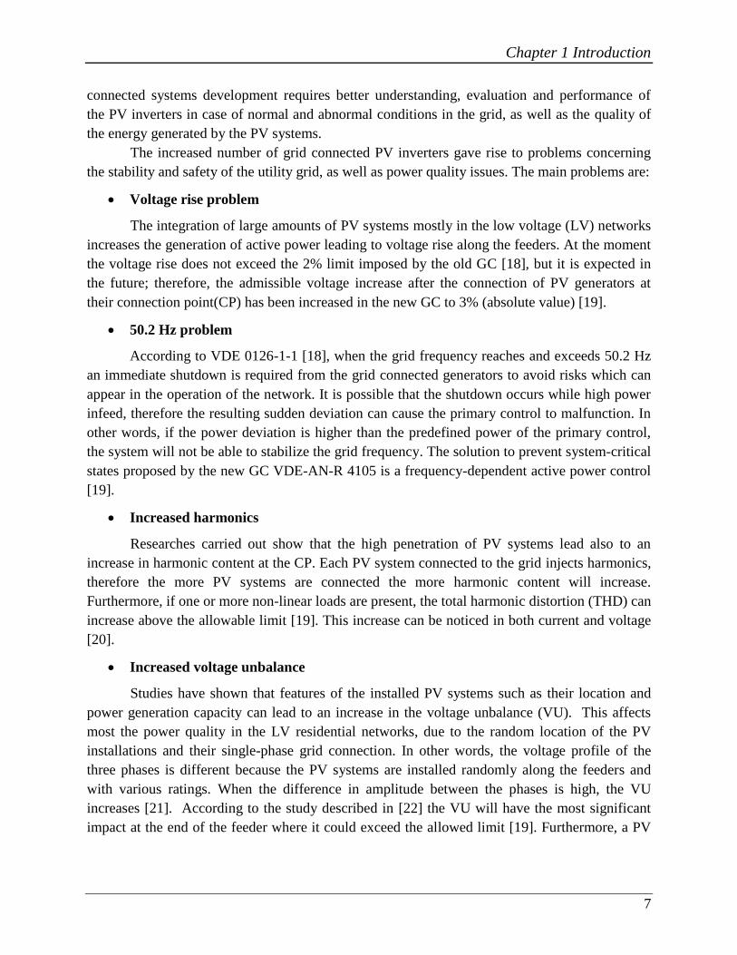
(loads connected during certain hours), temperature (appliances as air-conditioning dependant on
ambient temperature) and voltage (decrease of the voltage along the feeder as consequence of
reactive power consumption) [45].
Static Synchronous Compensator (STATCOM) is a Voltage Source Inverter (VSI)
connected to the grid for reactive power compensation and power factor improvement purposes
[46]. The most common configuration (see Figure 3-2) consists of VSI, DC-link capacitor, line
filter and coupling transformer [47]. Due to the shunt connection, STATCOM can be seen as a
current source; therefore, active and reactive power exchange between DS and STATCOM is
possible by controlling the magnitude and the phase angle of the output voltage of the VSI.
STATCOM device has the capability to sustain reactive current when the system
experience voltage variations. It also provides various additional advantages such as: voltage sag
mitigation, voltage stabilization, flicker suppression, power factor correction and harmonic
control. The voltage dip compensation is limited by the equivalent impedance of the power

Chapter 3 Voltage regulation strategies
23
system seen by the device, which is connected in parallel with the load impedance. In order to
minimize the losses, the STATCOM should be installed as close as possible to the load [46].
STATCOM LC Filter IL
VL
VSTATCOM
Vg
Figure 3-2 STATCOM connection to the utility grid [47]
3.3 Voltage regulation methods proposed by German GC VDE-AR-
N 4105
Reverse power flow in the electrical power grids limit the DG absorption capacity and
bring additional problems such as voltage rise and limited PV penetration. The problems can be
overcome by generation/absorption of reactive power by each PV inverter. The set power values
for each strategy are decided depending on the active power generation, voltage rise or
consumption profiles.[3, 48]
According to the new German GC, the voltage regulation methods for the PV generators
are the following:
Fixed power factor: cosφ method
Power factor characteristic: cosφ(P) method
Fixed Q reactive power method
Reactive power / voltage characteristic: Q(U) method
Both cosφ(P) and Q(U) strategies are based on droop characteristic. The fixed cosφ
method is suitable for systems where the active output generation is kept constant, otherwise, if
the active output is fluctuating, it is recommended to use one of the droop-based regulation
strategies. The fixed Q method assigns a reactive power reference for the PV generators based on
the network power flow investigation. Load power profile information and PV power production
are needed in order to in order to assign a reasonable fixed reactive power set values to the
inverters [49]. Furthermore, GCs encourage the use of load-flow calculations when determining
the voltage change values.
This project will further focus only on the droop-based regulations strategies because the
active generating output of the PV generators is fluctuating depending on the level of irradiation.
In all the cases, the voltage changes will be determined using load-flow analysis.

Control of grid connected PV systems with grid support functions
24
3.4 LV network analysis
The increased active power generation due to high PV penetration leads to voltage rise in
the network and can exceed the limit imposed by the GCs or can cause unexpected tripping of
other grid connected PV systems. Therefore, the PV capacity is limited and further investments
of transformer and lines upgrade are needed [49-54].
3.4.1 PV Inverter reactive power capability
The new regulations as German GC require from the PV inverters to inject or absorb
reactive power, depending on the grid status. The maximum and minimum value of reactive
power that an inverter can deliver is determined by its rated power (S) and active power from the
PV array PVP . When the active power produced equals with zero, the inverter can deliver
maximum reactive power and consequently, when PVP S , there is no reserve for reactive
power. Usually by over sizing the inverter with a 10 % it is enough to operate at power factor
equal with 0.9 (inductive or capacitive). Therefore, for future investigations, it is assumed that all
inverters have this capability [45].
Qinductive
Pm
ax
P
φ
Qcapacitive
Plim
Qmax
S max
Figure 3-3 Inverter capability of providing reactive power [25]
When operating at 0.9 power factor, the phase displacement between real and apparent
power will be:
180
cos(0.90) 25.84a
(3.1)
Maximum reactive power that the inverter is able to supply at rated power is:
max max 45.2%Q S (3.2)
In Figure 3-4, the inverter oversizing and reactive power supply capacity dependency is
illustrated.
Chapter 3 Voltage regulation strategies
25
10% 20% 30% 40%0%
Pact=100%Prated
10
20
30
40
50
60
70
80
90
100
80%
60%
40%
20%
Inverter Oversizing (Smax-Prated) [%Prated]
Rea
ctiv
e P
ow
er S
up
ply
Cap
acit
y [
%P
rate
d]
Figure 3-4 Reactive power supply capacity [ % ratedP ] depending on the inverter oversizing ( max ratedS P
)[48]
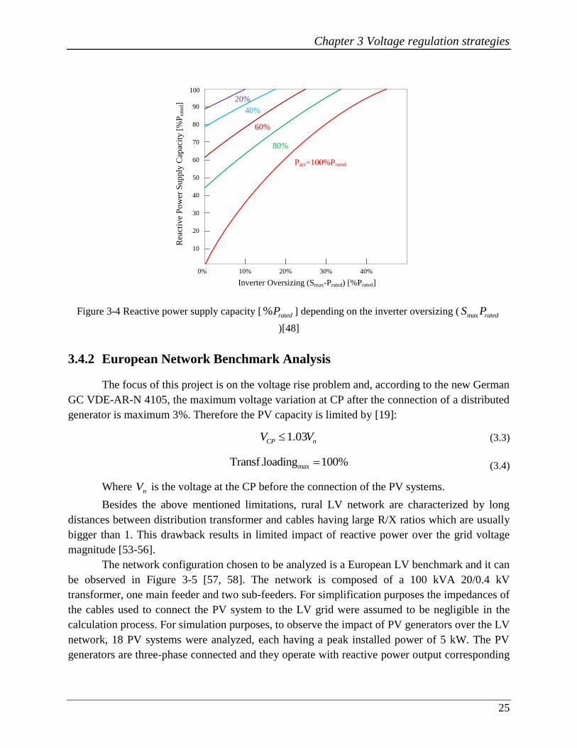
3.4.2 European Network Benchmark Analysis
The focus of this project is on the voltage rise problem and, according to the new German
GC VDE-AR-N 4105, the maximum voltage variation at CP after the connection of a distributed
generator is maximum 3%. Therefore the PV capacity is limited by [19]:
1.03CP nV V (3.3)
maxTransf.loading 100% (3.4)
Where nV is the voltage at the CP before the connection of the PV systems.
Besides the above mentioned limitations, rural LV network are characterized by long
distances between distribution transformer and cables having large R/X ratios which are usually
bigger than 1. This drawback results in limited impact of reactive power over the grid voltage
magnitude [53-56].
The network configuration chosen to be analyzed is a European LV benchmark and it can
be observed in Figure 3-5 [57, 58]. The network is composed of a 100 kVA 20/0.4 kV
transformer, one main feeder and two sub-feeders. For simplification purposes the impedances of
the cables used to connect the PV system to the LV grid were assumed to be negligible in the
calculation process. For simulation purposes, to observe the impact of PV generators over the LV
network, 18 PV systems were analyzed, each having a peak installed power of 5 kW. The PV
generators are three-phase connected and they operate with reactive power output corresponding

Control of grid connected PV systems with grid support functions
26
to a minimum power factor of 0.9. The distance between the PV generators was chosen to be
between 30m and 35m, depending on the LV topology.
Figure 3-5 European network benchmark [57]
The complete data of the LV network was taken from [58] and it can be found in Table 3-1.
Table 3-1 Rural LV network specifications [57, 58]
External Grid SSK=84.9 MVA; R=3.79 Ω; X=3.53 Ω
Distribution transformer S=100 kVA Dy5; 20/0.4 kV; ukr=4%; urr=2%
LV Branch Feeder conductor
(C11, C15, C16, C17, C18, C19)
NAYY 4x70 mm2 AL OLH; R=0.413 Ω/km;
X=0.3 Ω/km; length=0.3 km
LV Branch Feeder conductor
(C1, C2, C3, C4, C5, C7, C8, C9, C10, C12, C13,
C14)
NAYY 4x70 mm2 AL OLH; R=0.413 Ω/km;
X=0.3 Ω/km; length=0.35 km
MV Grid
Ssk=84.9 MVA
R=3.79Ω , X=3.53Ω
1
PV19
C19C1
C2
C3
C4
C12 C13
C17
20/0.4 kV
100 kVA
19
PV2
2
PV4
PV3PV11
C1111
3
4 12
PV12 PV13
13
C14
PV14
14
C15
PV15
15
C5
C7 C8
67
PV7 PV8
8
C9
PV9
9
C10
PV10
10
PV5
5
PV16
C1616
PV6
PV17
17
C18
PV18
18

Chapter 3 Voltage regulation strategies
27
The overhead cables between individual systems have impedance which resulted in an
R/X ratio of 1.37. Therefore, the active power has greater impact over the grid voltage and
causes voltage rise during high PV generation period. In this situation, the probability of voltage
violation is higher than in the other typical networks such as urban and suburban given the fact
that the character of those networks is more inductive. The voltage variation depending on active
and reactive current can be observer in the equation (3.5).
active reactiveV R I X I (3.5)
In order to determine the maximum PV capacity which can be installed in residential LV
networks and how PV systems are influencing the grid, test studies were performed using the
simulation software Power Factory from DigSILENT and MATLAB.
The considered input data in terms of active power production was chosen from a real
generation profile [59]. The measurements have a resolution of 15 min and they record the active
power generation of a residential PV system during a day with high irradiance in June 2007. For
the network presented in Table 3-1, 9 active power generation profiles were developed using the
data from [59]. Each generation profile was assigned to 2 PV systems. In Figure 3-6, the PV
generation profiles for one day in June 2007 are shown.
a) Profile 1 for PV2 & PV11 systems
b) Profile 2 for PV3 & PV12 systems
c) Profile 3 for PV4 & PV13 systems
d) Profile 4 for PV5 & PV14 systems

Control of grid connected PV systems with grid support functions
28
e) Profile 5 for PV6 & PV15 systems
f) Profile 6 for PV7 & PV16 systems
g) Profile 7 for PV8 & PV17 systems
h) Profile 8 for PV9 & PV18 systems
i) Profile 9 for PV10 & PV19 systems
Figure 3-6 Power generation profiles - June 2007 (a - i)
3.5 Load flow analysis
Load flow studies are performed to determine important features of power systems such
as: the magnitude and angle of the voltage in each bus and the active and reactive power flow in
each line. It also calculates the line losses and determines if the voltages remain within specified
limits and whether transformers are overloaded [60].
In order to mitigate the voltage rise problem on the chosen LV network, successive load
flow calculations are performed using the simulation software Power Factory from DigSILENT

Chapter 3 Voltage regulation strategies
29
[61]. This simulator uses Newton-Raphson method for load flow problem solving; therefore, this
algorithm will be explained and later implemented using MATLAB software.
Basically, the Newton-Raphson method calculates two unknown variables using the
known parameters and the power flow equations which include both types of variables and other
known parameters. Depending on the bus type, the unknown variables which can be calculated
based on the known variables are shown in Table 3-2.
Table 3-2 Known and unknown variables depending on bus type
Known variables Unknown variables
PQ bus Active and reactive power
(P, Q)
Voltage magnitude and angle
(|V|, δ)
PV bus Active power and voltage magnitude
(P, |V|)
Reactive power and voltage angle
(Q, δ)
Slack bus Voltage magnitude and angle
(|V|, δ)
Active and reactive power
(P, Q)
3.5.1 Newton-Raphson method
Further, the Newton-Raphson algorithm will be explained step by step [62] :
Step 1: Reading of data
The bus where the low-voltage side of the transformer is connected (CP1) was chosen to
be the slack bus and the rest are PQ buses.
Step 2: Construct the admittance bus (Ybus)
The busY is the matrix which contains all the admittances in the network. The form of the
matrix is the following:
111 12
221 22
1 2
1 , 19
N
N
bus
bus
N N NN
YY Y
YY YY N
Z
Y Y Y
(3.6)
Where:
iiY is the self-admittance (diagonal) and it is equal to the sum of the admittances of all the
branches connected to the thi node
ijY is the mutual admittance (off-diagonal) and is equal to the negative of the admittances
of all the branches connected between thi and
thj node

Control of grid connected PV systems with grid support functions
30
The impedance matrixbusZ is calculated based on the cable specifications from Table 3-1.
The values for all the elements of the busY matrix can be found in Appendix A.
Step 3: Start values
The start values refer to the initial conditions for the magnitude and angle of the voltages
in all CPs. Usually, when there are no other specifications, the flat start values are consider: 1
p.u. and 0 degrees.
The reference values for the active power generation are taken from [59] and the reactive
power reference is taken as 0.
Step 4: Number of iterations
The number of iteration is set to 3.
Step 5: Calculation of injected power
The active and reactive powers injected in all buses are calculated using the actual
magnitude and phase angles:
19
1
cos( )
i i j ij ij j i
j
P V V Y (3.7)
19
1
sin( )
i i j ij ij j i
j
Q V V Y (3.8)
A detailed description for calculating the above mentioned formulas is presented in
Appendix B.
Step 6: Difference between specified and injected power
The difference between the specified and the injected power values comes from the fact
that the injected powers are computed based on guessed values of voltage magnitude and angle
in the buses, whereas the specified ones are fixed reference values.
ref
i i iP P P (3.9)
ref
i i iQ Q Q
(3.10)
Step 7: Maximum difference
The power difference values is calculated and compared to a set tolerance value, in this
case 0.0001. If the mismatch is less than the tolerance, proceed to step 11, otherwise continue
with step 8.

Chapter 3 Voltage regulation strategies
31
Step 8: Jacobian matrix
The Newton-Raphson method is responsible with the linearization of the power equations
(3.9) and (3.10), therefore the Jacobian matrix is formed of partial derivatives that can be
computed. The active and reactive power corrections are found in Step 6. In this way, the
unknown variables, voltage magnitude and angle, can be calculated. The general form of the
Jacobian matrix is the following [62, 63]:
1 11 1
1 1
1
1 1
11 11 1
1 1
1 1
N N
N NN N
N N N
N N
N
N NN N
N N
Jacobian
P PP P
VV
P PP P
VV
VQ QQ Q
VV
V
Q QQ Q
VV
1
1
N
N
Corrections Mismatches
P
P
Q
Q
(3.11)
The form of the equation (3.11) can be simplified with the use of submatrixes:
'
'
i iik ik
i iik ik
PH N
V QJ L
(3.12)
The elements of the submatrixes ' ', , ,H J N L are the partial derivatives from (3.11)
which can be calculated taking into consideration also the bus type.
'
,
,
,
iik
k
iik
k
iik
k
PH i slack bus k slack bus
PN i slack bus k slack bus or PV bus
V
QJ i slack bus or PV bus k slack bus
'
iik
k
QL i slack bus or PV bus k slack bus or PV bus
V
(3.13)
The LV network analyzed in this project does not contain PV buses, therefore, only the
derivatives for the slack bus are not computed. The mismatches for the slack bus are not

Control of grid connected PV systems with grid support functions
32
considered since 1P and 1Q are undefined when 1P and 1Q are not scheduled and the
correction for 1 and 1V are both 0. In consequence, the dimensions of the submatrixes
' ', , ,H J N L are 1 1N N where N is the total number of buses in the network and in this
case is equal to 19.
In order to simplify the expression of the '
ikN and '
ikL submatrixes, their elements will be
multiplied with a voltage magnitude without influencing the result [63]. Therefore the correction
will become /i iV V and equation (3.12) can be rewritten in the following form:
/
ik ik i i
ik ik i i i
H N P
J L V V Q
(3.14)
The elements of the Jacobian matrix can now be calculated based on equations (3.7) and
(3.8).
when i k :
'
'
H = = V V sin cos
N = V N =V = V V cos sin
= = V V cos sin
L = V =V = V V sin cos
iik i k ik ik ik ik
k
iik k ik k i k ik ik ik ik
k
iik i k ik ik ik ik
k
iik k ik k i k ik ik ik ik
k
PG B
PG B
V
QJ G B
PL G B
V
(3.15)
when i k :
2
2
2
2
H =
N = P
= P
L =
ii i ii i
ii i ii i
ii i ii i
ii i ii i
Q B V
G V
J G V
Q B V
(3.16)
A more detailed description of how the Jacobian matrix is formed and how its elements
are computed can be found in [63] .
Step 9: Calculation of ΔV and Δδ
Using the power mismatches calculated at Step 6 and the elements of the Jacobian matrix
computed at Step 8, the corrections can be found using the following formula:

Chapter 3 Voltage regulation strategies
33
1
/
i ik ik i
i i ik ik i
H N P
V V J L Q
(3.17)
Step 10: New voltage magnitude and angle
Using the calculated corrections in Step 9, the new voltages can be computed using
equations (3.18) and (3.19).
1 / i i i iV V V V i slack bus (3.18)
i i i i slack bus (3.19)
Step 11: Power flow and power production
The active and reactive power flows and the net power production in all busses can be
calculated with the known voltage magnitude and angle values. Furthermore, the total network
losses can also be computed.
3.5.2 Load flow results
The first load flow analysis on the chosen LV network must be performed with the
following conditions: maximum active power generation and no reactive power consumption.
The purpose of this study is to examine the maximum voltage levels in the network and based on
these values, a reactive power compensation strategy can be proposed. Furthermore, based on the
measured values, the droop characteristics can be developed for both regulation methods
proposed by the German GC VDE-AR-N 4105 [19].
To emphasize the voltage increase due to PV power generation, a study case with zero
load demand was considered. The voltage value at the slack bus before the connection of the PV
systems is chosen 1 p.u.. In Figure 3-7, the network voltage levels at all CPs are presented. As
expected, the network experience voltage rise above the 3% limit with the maximum rise at the
end of the feeder.
a) Voltage level at CP1
b) Voltage level at CP2
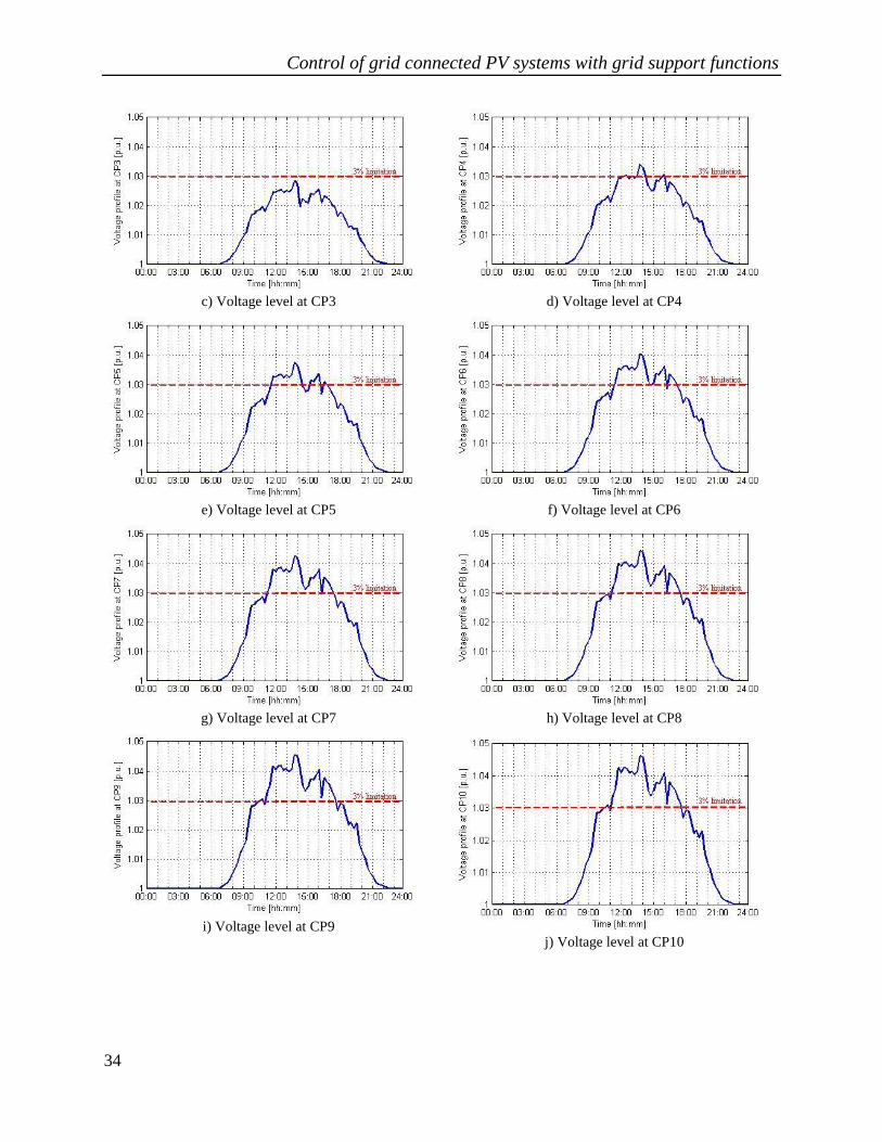
Control of grid connected PV systems with grid support functions
34
c) Voltage level at CP3
d) Voltage level at CP4
e) Voltage level at CP5
f) Voltage level at CP6
g) Voltage level at CP7
h) Voltage level at CP8
i) Voltage level at CP9
j) Voltage level at CP10

Chapter 3 Voltage regulation strategies
35
k) Voltage level at CP11
l) Voltage level at CP12
m) Voltage level at CP13
n) Voltage level at CP14
o) Voltage level at CP15
p) Voltage level at CP16
q) Voltage level at CP17
r) Voltage level at CP18

Control of grid connected PV systems with grid support functions
36
s) Voltage level at CP19
Figure 3-7 Voltage levels at all CPs of the network after performing the load flow analysis (a - s)
In order for the whole system to be inbounded to the 3% voltage limit and to avoid power
curtailment, PV generators have to adopt voltage regulation methods.
The transformer loading also calculated after performing the load flow analysis for one
day in June 2007 can be seen in Figure 3-8. As it can be observed, the loading level does not
exceed 100%.
Figure 3-8 Transformer loading when no voltage regulation methods are applied
The source code developed using DigSILENT simulator for the load flow analysis can be
found in Appendix C.
3.6 Cosφ(P) method
The first voltage regulation method proposed by the German GC is calculating the
reactive power reference depending on the active power generated by the PVs (Figure 3-9).
When the power production is low, the risk of overvoltage in the network is small as well. When
the power generation increase reaches half of the PV nominal power, the power factor is
decreasing towards 0.9 and reactive power is absorbed.

Chapter 3 Voltage regulation strategies
37
The method does not use grid voltage information and is only assuming that high power
generation matches the voltage increase [49, 58].
Figure 3-9 Droop characteristic for cosφ (P) method
The main drawback of this method is the possibility of reactive power consumption even
though the voltage at the CP is in admissible range. Furthermore, this method does not take into
consideration the impedance of the cables and the PV system located nearest to the transformer
can absorb the same amount of reactive power as the PV system located at the end of the feeder
if they both have the same active power generation [49, 58].
In this case the reactive power reference can be expressed as:
Q tan( acos ) P (3.20)
The maximum reactive power the PV inverter can absorb at the rated power of 5kW is:
0 9 2 42max nQ tan( acos( . )) P . kVar (3.21)
The flow chart presented in Figure 3-10 shows the implementation of the cosφ(P)
algorithm on the chosen LV network.
The first step consists of assigning the active power reference value (ref
iP ). The data will
be assigned each 15 minutes during a day; therefore a total of 96 assignments will be performed.
Next, the algorithm checks the value of the active power generation value to assign its
corresponding cosφ value and calculate the reactive power consumption. If the ref
iP value is less
than half the rated power ( nP 5kW ), the system works at unitary PF and no reactive power is
consumed. If the power reference is higher than the nominal value, the system absorbs the
maximum amount of reactive power ( maxQ 2.42kVar ). For any other values of ref
iP a
corresponding value for PF is assigned according to Table 3-3 and the reactive power reference ref
iQ is calculated. The algorithm stops when the number of iterations set by user is reached.
cosφ
1
Pn
0.90.5Pn
ind
uct
ive
cosφ
Pn
Closer to the transformer
PV1 PV2 PV19
PV1, PV2…PV19

Control of grid connected PV systems with grid support functions
38
Start
YES
NO
Assign ref Pi value
YES
NO
ref Pi < 0.5Pn? cosφ = 1
Assign ref
Pi = 0
Calculate
Load Flow
refPi > Pn?
NO
YES Assign refQi = Qmax
Calculate
Load Flow
ref Check Pi interval
0.5Pn -> Pn
Assign cosφ
cosφ = 1 -> 0.9
ref Calculate Qi
ref Qi = tan(acos(cosφ ))
Calculate
Load Flow
Last
Iteration?Stop
Figure 3-10 Flow chart with the implementation of the cosφ(P) method
Table 3-3 Cosφ values assigned corresponding to ref
iP values when ref
iP [2.5;5]kW
ref
iP interval
(kW) [2.5, 2.75] (2.75, 3] (3, 3.25] (3.25, 3.5] (3.5, 3.75]
cosφ 0.99 0.98 0.97 0.96 0.95
ref
iP interval
(kW) (3.75, 4] (4, 4.25] (4.25, 4.5] (4.5, 4.75] (4.75, 5]
cosφ 0.94 0.93 0.92 0.91 0.9
The source code developed using DigSILENT simulator to implement the cosφ(P)
method can be found in Appendix D.
3.7 Q(U) method
The second strategy of voltage regulation proposed by the German GC, presented in
Figure 3-11, is calculating the reactive power reference of each PV system depending on the
voltage magnitude measured at its corresponding CP. The benefit of this method compared to

Chapter 3 Voltage regulation strategies
39
cosφ(P) is that it uses local voltage information in the regulation process which means the
reactive power consumption will be proportional to the voltage level.
The main drawback of this regulation method is the improper use of the inverter available
capacity. It is likely the voltage magnitude at the CPs near the transformer to be within limits,
therefore the corresponding PV systems will not participate in the regulation process, making the
task much difficult for the other PV inverters. Furthermore, the probability that the inverters
situated further away from the transformer will work at full capacity or at a capacity higher than
the inverters located near the transformer. Because each PV system performs a local regulation
process, the inverters with available capacity cannot help the inverters working at full capacity;
therefore, in terms of reliability, the inverters located at the end of the feeder will experience
reliability problems earlier [50, 58, 64].
As stated in the German GC, the droop curve for the Q(U) method is provided by the
network operator. Therefore, the droop characteristic specific for the LV network studied in this
project must be designed. Based on the results of the first load flow analysis, for the maximum
voltage value, the corresponding reactive power absorption value can be assigned. As it can be
seen from Figure 3-11, this value can be taken as 1.05 p.u. because when there is no reactive
power absorption in the network, the maximum voltage magnitude does not exceed 1.05 p.u..
The start value for absorbing reactive power is chosen to be 1.02 p.u.. Using these values, the
droop characteristic can be achieved and the Q(U) regulation method can be implemented
(Figure 3-12) [58].
Q [kVar]
1
-Qmax
Q [kVar]
Closer to the transformer
PV19 PV18
1.02 1.05V [p.u.]
0.980.95
Qmax
V [p.u.]2 3 4 17V1 V2 V3 V4
Figure 3-11 Droop characteristic for Q(U) method
The voltage variation is calculated using the following formula:
3
3
34 [%] , 0,1measV V
V
(3.22)
The reactive power reference is calculated using the value of the voltage variation found
in (3.20):
max
ref
iQ Q (3.23)
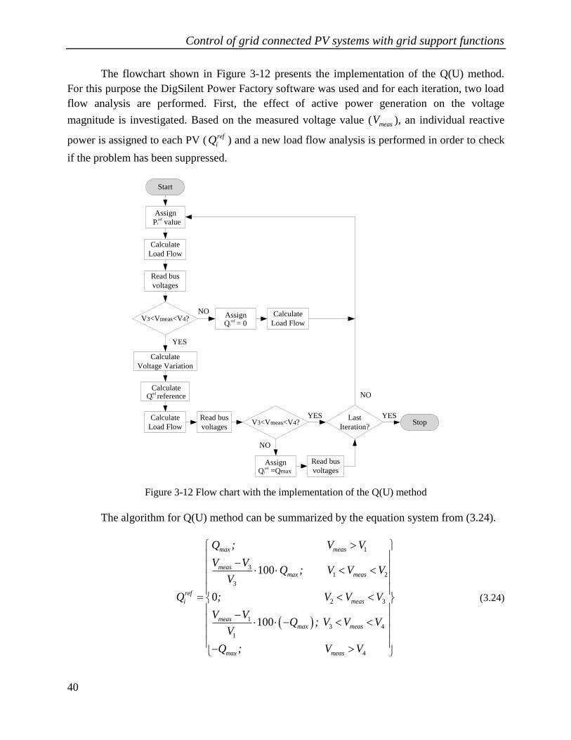
Control of grid connected PV systems with grid support functions
40
The flowchart shown in Figure 3-12 presents the implementation of the Q(U) method.
For this purpose the DigSilent Power Factory software was used and for each iteration, two load
flow analysis are performed. First, the effect of active power generation on the voltage
magnitude is investigated. Based on the measured voltage value ( measV ), an individual reactive
power is assigned to each PV (ref
iQ ) and a new load flow analysis is performed in order to check
if the problem has been suppressed.
Start
Assign ref Pi value
Calculate
Load Flow
Read bus
voltages
V3<Vmeas<V4?
YES
NOAssign
ref Qi = 0
Calculate
Load Flow
Calculate
Voltage Variation
Calculate ref Qi reference
Calculate
Load Flow
Read bus
voltagesV3<Vmeas<V4?
NO
Assign refQi =Qmax
YES
Read bus
voltages
Last
Iteration?
YESStop
NO
Figure 3-12 Flow chart with the implementation of the Q(U) method
The algorithm for Q(U) method can be summarized by the equation system from (3.24).
1
31 2
3
2 3
13 4
1
100
0
100
max meas
measmax meas
ref
i meas
measmax meas
max
Q ; V V
V VQ ; V V V
V
Q ; V V V
V VQ ; V V V
V
Q ;
4meas V V
(3.24)

Chapter 3 Voltage regulation strategies
41
It can be mentioned that for the LV network studied in this project, the only concern is
the voltage rise problem and PV systems are required only to absorb reactive power, therefore
only the corresponding part from the equation system was considered for implementation. The
source code developed using DigSILENT simulator to implement the Q(U) method can be found
in Appendix E.
3.8 Study case results
The performance of the above described methods is investigated based on voltage level,
reactive power flow and the transformer loading level. First, the behavior of the PV systems
closer to the transformer is investigated. It is expected that these systems will experience less
voltage rise at their CPs. When the selected voltage regulation strategies are implemented, each
PV system consume a reactive power value corresponding to its active power generation (cosφ
(P)) or the local voltage magnitude (Q(U)).
In Figure 3-13a) the voltage profile of the closest system to the transformer (PV19) is
shown. As it can be observed the highest voltage level at the CP is around 1.015p.u.. In Figure
3-13b), the generation profile of the PV19 generator is presented together with the levels of
reactive power consumed using both regulation methods. The reason there is no reactive power
absorption for Q(U) strategy is because the droop-characteristic, defined in Figure 3-11, states
that the inverter will start consuming reactive power only when the voltage reaches the value of
1.02 p.u. For this PV system the voltage remains inside the dead band of the droop curve
(0.98p.u. – 1.02p.u.). On the other hand, it can be observed that the cosφ(P) algorithm consumes
large amounts of reactive power, proportional to the active generation levels, even though no
voltage regulation is needed. Although the voltage is between limits, the high amount of reactive
absorption leads to a decrease in voltage level to an approximate value of 1.005 p.u..
a)
b)
Figure 3-13 PV19 system analysis a) Voltage levels with and without regulation methods b) Active power
generation and reactive power consumed using regulation methods
The reason the voltage at the CP19 when using the Q(U) algorithm is lower compared to
the voltage when no regulation is applied in the network is due to the influence of the reactive
power absorbed by the rest of the network and the high impedance of the transformer.
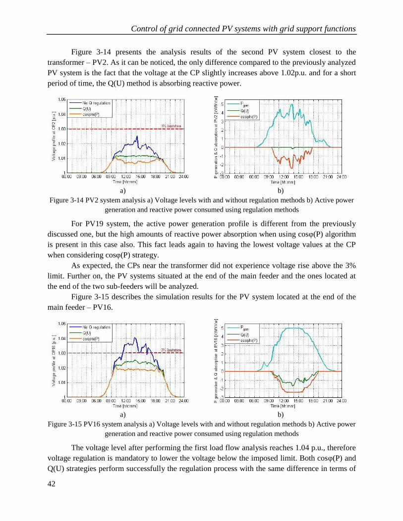
Control of grid connected PV systems with grid support functions
42
Figure 3-14 presents the analysis results of the second PV system closest to the
transformer – PV2. As it can be noticed, the only difference compared to the previously analyzed
PV system is the fact that the voltage at the CP slightly increases above 1.02p.u. and for a short
period of time, the Q(U) method is absorbing reactive power.
a)
b)
Figure 3-14 PV2 system analysis a) Voltage levels with and without regulation methods b) Active power
generation and reactive power consumed using regulation methods
For PV19 system, the active power generation profile is different from the previously
discussed one, but the high amounts of reactive power absorption when using cosφ(P) algorithm
is present in this case also. This fact leads again to having the lowest voltage values at the CP
when considering cosφ(P) strategy.
As expected, the CPs near the transformer did not experience voltage rise above the 3%
limit. Further on, the PV systems situated at the end of the main feeder and the ones located at
the end of the two sub-feeders will be analyzed.
Figure 3-15 describes the simulation results for the PV system located at the end of the
main feeder – PV16.
a)
b)
Figure 3-15 PV16 system analysis a) Voltage levels with and without regulation methods b) Active power
generation and reactive power consumed using regulation methods
The voltage level after performing the first load flow analysis reaches 1.04 p.u., therefore
voltage regulation is mandatory to lower the voltage below the imposed limit. Both cosφ(P) and
Q(U) strategies perform successfully the regulation process with the same difference in terms of

Chapter 3 Voltage regulation strategies
43
reactive power consumption: the amount absorbed with cosφ(P) is significantly higher than using
Q(U).
The analysis of the simulation results continue with the PV system located at the end of
the first sub-feeder - PV15. As well as the previous analyzed system, the voltage level at the CP
violates the 3% limit and after the regulation process the voltage is reduced and maintained in the
specific range (Figure 3-16).
a)
b)
Figure 3-16 PV15 system analysis a) Voltage levels with and without regulation methods b) Active power
generation and reactive power consumed using regulation methods
Finally, the PV system situated at the end of the second sub-feeder and furthest away
from the transformer is discussed – PV18 (Figure 3-17). The highest voltage level in the
network, approximately 1.046, is reached at the CP of this system. The interesting part is that in
this case the roles are reversed and the Q(U) method consumes more reactive power than cosφ(P)
in the first part of the day until around 15:00. The reason this happened is the low levels of active
power generation.
a)
b)
Figure 3-17 PV18 system analysis a) Voltage levels with and without regulation methods b) Active power
generation and reactive power consumed using regulation methods
In Figure 3-18, the transformer loading for the analyzed strategies is shown. Without the
reactive power regulation from the PV systems, the maximum transformer loading is 81%. The
Q(U) method minimizes the reactive power absorption and increases the loading of the

Control of grid connected PV systems with grid support functions
44
transformer to a maximum value of 85.5%. On the other hand, the cosφ(P) method limits the
further PV capacity achievement due to the high amounts of reactive power consumption which
lead to a 91% loading of the transformer.
Figure 3-18 Transformer loading for the analyzed strategies
3.9 Discussions
The performance of both cosφ(P) and Q(U) regulation methods was evaluated on the
chosen European LV network based on their ability to maintain the voltage between specified
limits.
The purpose of having more active power generation profiles for the PV systems is to
emphasize the effect of the cosφ(P) method. If all PV generators had the same profile, the
amount of reactive power consumed using cosφ(P) would have been the same for all the
inverters.
The simulation results show that both methods have achieved their regulation purpose.
Although the voltage values using the cosφ(P) are closer to 1 p.u. compared to Q(U) method, the
consequence of having a lower voltage is a higher reactive power consumption. As long as the
voltage does not exceed the 3% limit, the value is not an issue, therefore the fact that the voltage
level is lower using cosφ(P) cannot be seen as an advantage because it does not have any effect
on the network.
The difference between the two strategies in terms of reactive power is prominent as both
strategies calculate the reactive power consumption in two different ways. Because cosφ(P)
method does not consider any feedback from the network nor the voltage sensitivity, all the
inverters in the network can consume the same amount of reactive power, regardless of their
position and the voltage levels. On the other hand, Q(U) method takes into consideration the
above mentioned issues and improves the inverter capacity use. The inverters that do not
experience voltage rise over the limit are not as stressed as the other inverters and the reactive
power consumption is therefore decreased. From the point of view of reactive power absorption,
it can be stated that Q(U) method is better, but improvements can be made so that all inverters
can participate in the regulation process with their available capacity.

Chapter 3 Voltage regulation strategies
45
From the above mentioned, another conclusion can be drawn in terms of reliability.
Because of the higher levels of reactive power consumed by all the inverters with cosφ(P)
method, the amount of inverters that can experience problems is bigger than in case of using
Q(U) strategy; thus leading to a lower life-time of the inverters.
The last performance criterion to evaluate the two control strategies is the level of
transformer loading. The simulation results shown that the transformer loading was most
increased when using the cosφ(P). It is normal because the higher stress on the transformer is the
consequence of the larger amounts of reactive power absorption.
Both methods proposed by the new German GC VDE-AR-N 4105 were implemented on
a LV network and analyzed from different points of view. All the results and discussions point in
the same direction: the Q(U) algorithm is the best candidate when considering voltage regulation
in a LV network with minimum reactive power consumption.


Chapter 4 Improved voltage regulation strategies
47
Chapter 4 Improved voltage regulation
strategies
The chapter describes an optimization algorithm for voltage regulation in LV network in
order to improve the classical methods proposed by the German GC. The implementation of the
optimized Q(U) algorithm is explained in detail and simulation results are discussed and
compared with the classical Q(U) algorithm which was chosen as best candidate based on the
results from the previous chapter.
4.1 Optimized Q(U) method
The main objectives when talking about networks are to find optimal solutions to problems
that minimize the costs. The optimization problem treated in this chapter refers to the reactive
power dispatch problem with the focus on developing an algorithm with the following purposes:
Maintain the voltages at the CPs below the specified limit
Minimize the reactive power consumption of the overall network, hence minimize the
losses in the line
Use the available capacity of all the PV inverters to avoid stressing the ones at the end of
the feeder
Use advanced communication protocols to gather information from all the PV systems on
a centralized controller which would calculate the optimal reactive power reference for
each PV system
4.1.1 Standard optimization problem
Optimization is a mathematical process in which a search is activated that aims at a best
value of an objective function that is optimal [65] . In general , an optimization algorithm has a
specific objective function to be minimized while satisfying some predefined equality and
inequality constraints.
The objective functions are formed based on a problem definition. In general, there are
various features in a network that can be considered problems which can be optimized, for
example: minimization of the total generating cost, reduction of active transmission losses,
security and stability of the power system [66, 67] . Each of these problems can be define to form
the objective function of an optimization algorithm. The standard form of the objective function
is ( )F x where F is a scalar function and x is the vector of the design variables containing both
state and control variables. The state variables describe any unique state of the power system,
whereas the control variables can be modified to satisfy predefined conditions .
Control of grid connected PV systems with grid support functions
48
For any optimization problem, the equality constrains are expressed using the form
( ) 0g x where g is a function assumed to be continuous and at least twice differentiable [68] .
The most common equality constraints for power systems refer to the nonlinear load flow
equations. These constraint functions contain the limits for the state variables.
The inequality constraint function has the form ( ) 0h x . Usually, these functions define
some specific bounds such as: voltage levels at the CP in a network, transmission line flow limit,
reactive power capabilities of inverters etc.
Therefore, the standard form of the optimization problem can be expressed as:
min ( )F x (4.1)
Subject to:
( ) 0g x (4.2)
( ) 0h x
(4.3)
4.1.2 Problem formulation process for the LV network
In this subchapter, the problem formulation process will be presented step by step based
on [69] :
Step 1: Problem Statement
Maintain the voltage levels at all the CPs of the LV network between limits imposed by
the German GC considering in the same time the optimization of the reactive power dispatch.
Step 2: Data and Information Collection
the number of PV systems in the network is 18
the considered CPs are beginning from the LV-side of the transformer and the total
number is 19 (1 slack bus and 18 PQ buses)
the influence of the transformer impedance is not taken into consideration (Figure 4-1)
active power generation profile of all PV generators are predefined
inverter capabilities in terms of active and reactive power are set
parameters for cables are predefined
Step 3: Identification/Definition of the design variables
The state variables consist of the voltage magnitude iV and angle i for each bus in
the LV network. The reactive power references ref
iQ of all PV systems are defined as the
control variables. Both set of variables have the following vector form:
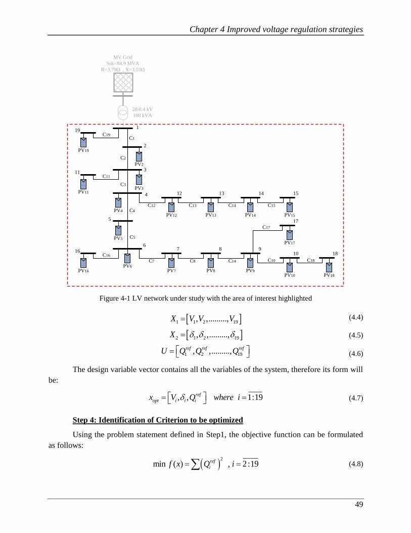
Chapter 4 Improved voltage regulation strategies
49
MV Grid
Ssk=84.9 MVA
R=3.79Ω , X=3.53Ω
1
PV19
C19C1
C2
C3
C4
C12 C13
C17
20/0.4 kV
100 kVA
19
PV2
2
PV4
PV3PV11
C1111
3
4 12
PV12 PV13
13
C14
PV14
14
C15
PV15
15
C5
C7 C8
67
PV7 PV8
8
C14
PV9
9
C10
PV10
10
PV5
5
PV16
C1616
PV6
PV17
17
C18
PV18
18
Figure 4-1 LV network under study with the area of interest highlighted
1 1 2 19, ,.........,X V V V (4.4)
2 1 2 19, ,.........,X
(4.5)
1 2 19, ,.........,ref ref refU Q Q Q
(4.6)
The design variable vector contains all the variables of the system, therefore its form will
be:
, , 1:19ref
opt i i ix V Q where i (4.7)
Step 4: Identification of Criterion to be optimized
Using the problem statement defined in Step1, the objective function can be formulated
as follows:
2
min ( ) , 2 :19ref
if x Q i (4.8)

Control of grid connected PV systems with grid support functions
50
Step 5: Identification of Criterion to be optimized
Step 5.1: Identification of Equality Constraints
As stated before, the power flow equations are used as equality constraints:
19
1
1
cos sin 0 , 2 :19ref
i i j ij ij ij ij
j
g P V V G B i
(4.9)
19
2
1
sin cos 0 , 2 :19ref
i i j ij ij ij ij
j
g Q V V G B i
(4.10)
Where ,i jV V are the voltages at i and j buses, 2 :19i , 1:19j . ,ref ref
i iP Q are the active
and reactive power injected at bus i. ,ij ijG B are the conductance and susceptance between bus i
and j and ij is the voltage angle difference between bus i and j.
The equality constraint for the slack bus refers to the reactive power reference, voltage
magnitude and angle:
1 1
1 3 1
1 1
0 0
1 . . 1 0
0 0
ref refQ Q
V p u g V
(4.11)
Step 5.2: Identification of Inequality Constraints
First inequality constraint expresses the limits for voltage magnitude for all PQ buses in
the network:
1
0.97 00.97 . . 1.03 . . , 2,19
1.03 0
i
i
i
Vp u V p u h i
V
(4.12)
Moreover, the reactive power capabilities of the PV inverters are limited:
2 2 2 2
2 2
2 0 , 2,19ref ref ref ref
i i i i i iP Q S h P Q S i (4.13)
It should be mentioned that a minimization of line losses is also achieved with the load
flow equations taken as constraints and the use of fmincon function.
Step 6: Initial Conditions
The initial condition for voltage magnitude and angle are the output values of the first
load flow performed for the LV network and zero for the reactive power references.
_ _
, , 0 , 1:19load flow load flow init init
ref ref
init i i i ix V Q where Q i
(4.14)
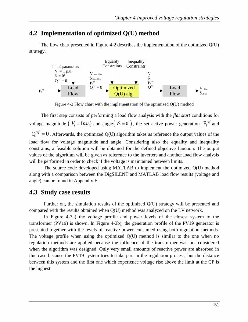
Chapter 4 Improved voltage regulation strategies
51
4.2 Implementation of optimized Q(U) method
The flow chart presented in Figure 4-2 describes the implementation of the optimized Q(U)
strategy.
Vi = 1 p.u.δi = 0° refQi = 0
Initial parameters
refPi
Viload_flow
δiload_flow refPi refQi = 0
Vi
δi
refPi refQi
Equality Constraints
Inequality Constraints
Load
Flow
Optimized
Q(U) alg.
Load
FlowVi_final
δi_final
Figure 4-2 Flow chart with the implementation of the optimized Q(U) method
The first step consists of performing a load flow analysis with the flat start conditions for
voltage magnitude 1 . .iV p u and angle 0i , the set active power generation Pref
i and
Q 0ref
i . Afterwards, the optimized Q(U) algorithm takes as reference the output values of the
load flow for voltage magnitude and angle. Considering also the equality and inequality
constrains, a feasible solution will be obtained for the defined objective function. The output
values of the algorithm will be given as reference to the inverters and another load flow analysis
will be performed in order to check if the voltage is maintained between limits.
The source code developed using MATLAB to implement the optimized Q(U) method
along with a comparison between the DigSILENT and MATLAB load flow results (voltage and
angle) can be found in Appendix F.
4.3 Study case results
Further on, the simulation results of the optimized Q(U) strategy will be presented and
compared with the results obtained when Q(U) method was analyzed on the LV network.
In Figure 4-3a) the voltage profile and power levels of the closest system to the
transformer (PV19) is shown. In Figure 4-3b), the generation profile of the PV19 generator is
presented together with the levels of reactive power consumed using both regulation methods.
The voltage profile when using the optimized Q(U) method is similar to the one when no
regulation methods are applied because the influence of the transformer was not considered
when the algorithm was designed. Only very small amounts of reactive power are absorbed in
this case because the PV19 system tries to take part in the regulation process, but the distance
between this system and the first one which experience voltage rise above the limit at the CP is
the highest.

Control of grid connected PV systems with grid support functions
52
a)
b)
Figure 4-3 PV19 system analysis a) Voltage levels with and without regulation methods b) Active power
generation and reactive power consumed using regulation methods
Similar results are shown in Figure 4-4 for PV2 system compared with PV19 system
because the difference between them is the length of the cables. PV19 system is connected
directly to the rest of the system, therefore it takes part in the regulation process with slightly
higher amounts of reactive power absorption compared with the previous system, but they are
still low compared to the other systems.
a)
b)
Figure 4-4 PV2 system analysis a) Voltage levels with and without regulation methods b) Active power
generation and reactive power consumed using regulation methods
In order to see the improvements brought by the optimized Q(U) algorithm the systems
located at the end of the main feeder and the two sub-feeders will be presented further on.
Figure 4-5 describes the simulation results for the PV system located at the end of the
main feeder – PV16. Although there is a difference between the voltages after performing the
regulation strategies, both perform successfully the regulation process, but the reactive power
amount absorbed with the optimized Q(U) algorithm is lower than using Q(U).

Chapter 4 Improved voltage regulation strategies
53
a)
b)
Figure 4-5 PV16 system analysis a) Voltage levels with and without regulation methods b) Active power
generation and reactive power consumed using regulation methods
The analysis of the simulation results continue with the PV systems located at the end of
the two sub-feeders - PV15 and PV18 (Figure 4-6 and Figure 4-7).
a)
b)
Figure 4-6 PV15 system analysis a) Voltage levels with and without regulation methods b) Active power
generation and reactive power consumed using regulation methods
a)
b)
Figure 4-7 PV18 system analysis a) Voltage levels with and without regulation methods b) Active power
generation and reactive power consumed using regulation methods
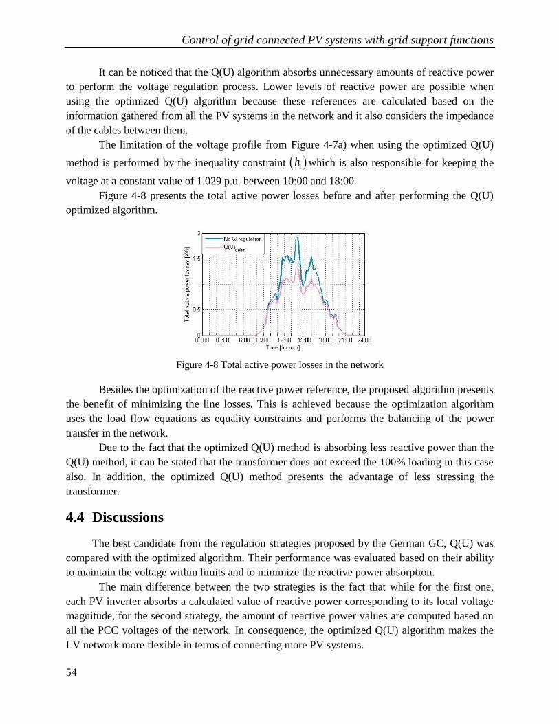
Control of grid connected PV systems with grid support functions
54
It can be noticed that the Q(U) algorithm absorbs unnecessary amounts of reactive power
to perform the voltage regulation process. Lower levels of reactive power are possible when
using the optimized Q(U) algorithm because these references are calculated based on the
information gathered from all the PV systems in the network and it also considers the impedance
of the cables between them.
The limitation of the voltage profile from Figure 4-7a) when using the optimized Q(U)
method is performed by the inequality constraint 1h which is also responsible for keeping the
voltage at a constant value of 1.029 p.u. between 10:00 and 18:00.
Figure 4-8 presents the total active power losses before and after performing the Q(U)
optimized algorithm.
Figure 4-8 Total active power losses in the network
Besides the optimization of the reactive power reference, the proposed algorithm presents
the benefit of minimizing the line losses. This is achieved because the optimization algorithm
uses the load flow equations as equality constraints and performs the balancing of the power
transfer in the network.
Due to the fact that the optimized Q(U) method is absorbing less reactive power than the
Q(U) method, it can be stated that the transformer does not exceed the 100% loading in this case
also. In addition, the optimized Q(U) method presents the advantage of less stressing the
transformer.
4.4 Discussions
The best candidate from the regulation strategies proposed by the German GC, Q(U) was
compared with the optimized algorithm. Their performance was evaluated based on their ability
to maintain the voltage within limits and to minimize the reactive power absorption.
The main difference between the two strategies is the fact that while for the first one,
each PV inverter absorbs a calculated value of reactive power corresponding to its local voltage
magnitude, for the second strategy, the amount of reactive power values are computed based on
all the PCC voltages of the network. In consequence, the optimized Q(U) algorithm makes the
LV network more flexible in terms of connecting more PV systems.
Chapter 4 Improved voltage regulation strategies
55
Even though the voltage levels using the optimized Q(U) method are higher, but within
limits compared to the voltage using the Q(U) algorithm, the benefit of the optimized method is
the minimization of the reactive power absorption while the PV generators maintain their
operation in MPPT.
Other benefits of the optimized Q(U) method over the classical Q(U) are the
minimization of the line losses and lower transformer loading.
Both methods were implemented on a LV network and analyzed from different points of
view. All the results and discussions conclude that the optimized Q(U) algorithm has improved
the classical Q(U) method proposed by the new German GC VDE-AR-N 4105.

Chapter 5 Voltage regulation strategies using the communication concept
57
Chapter 5 Voltage regulation strategies
using the communication
concept
The chapter presents the analysis of the standards series IEC 61850 together with its
experimental validation. In the beginning, an overview of how the standard is structured and a
general description of the information model are given. Further on, the experimental setup and
the methodology of implementation are presented along with the results.
5.1 Analysis of the IEC 61850 standard
5.1.1 Introduction
The massive integration of renewable energy into the utility grid lead to the necessity of
developing modern electricity systems. The new technology based on real-time information
exchange, also known as “Smart Grid Concept” aims to optimize the energy power supply and
demand by taking advantage of the computing and communication concept. This big task implies
changes in the control algorithms and a new configuration of the network which allows two-way
data information exchange thus resulting in a well-organized DG integration without affecting
the power flow efficiency [70].
One of the biggest challenges to overcome in the development of smart grid systems was
the interoperability between intelligent electronic devices (IEDs). Power system equipments
which incorporate microprocessor-based controllers such as circuit breakers, transformers,
converters, capacitor banks etc. and can exchange information are defined as IEDs. Very often,
devices of different manufactures couldn‟t interoperate due to compatibility issues and missing
communication standard, and therefore the task of implementing a communication system
became difficult and complicate. In order to overcome the limitations stated above, the working
groups of the Technical Committee 57 of IEC (IEC TC57) issued a new standard IEC 61850
which regulates the communication in substations and defines a common information exchange
protocol between interconnected IEDs. In this way, the Smart Grid technology along with its
automation and control functions can be integrated into power systems, resulting in benefits for
the grid operator [71].
In electric power systems, the management of information and protection functions is
done into substations (known as nodes) which include transformers, switching and protection
devices. It is the place where the lines and cables are connected for transmission and distribution
of electric power. In a substation automation system (SAS) the information can be accessed over
the network (eg. TCP/IP) and in consequence the human intervention can be reduced to

Control of grid connected PV systems with grid support functions
58
minimum. The modeling approach is to create a model which comprises all the components
defined as IEDs and their functions, by including also the form of communication allowed by the
system [72, 73].
5.1.2 Overview and Scope of IEC 61850
The IEC 61850 standard series named “Communication networks and systems in
substations” comprises in total 10 major sections, which cover different aspects of the substation
communication network. In Figure 5-1, the modeling and implementation methods applied in the
parts of the standard are exposed [74].
Introduction
IEC 61850-1
Glossary
IEC 61850-2
Technical report
---Guidelines
---IEC
61850-90-xx
Configuration
description
language
IEC
61850-6
Application guide
IEC 61850-7-5xx
Application guide
IEC 61850-7-5
Compatible LN and
Data classes
IEC 61850-7-4
Domain specific LN
and Data classes
IEC 61850-7-4xx
Common Data Classes
IEC 61850-7-3
Basic models, abstract services and basic types
IEC 61850-7-2
Principles
and models
IEC
61850-7-1
Communication
requirement for
devices and
functions
IEC
61850-5
Mapping on network
(except sample values)
IEC 61850-8-xx
Sample Values mapping
on network
IEC 61850-9-xx
Implementation
Conformance testing
IEC 61850-10
System and project
management
IEC 61850-4
General requirements
IEC 61850-3
Figure 5-1 Relations between modeling and mapping parts of the IEC 61850 series [74]
The parts 1 and 2 are meant to provide an introduction to the standard series IEC 61850
and contain also the glossary of terms used along with definitions regarding the power utility
automation systems context. The general requirements for communication in substations are
presented in part 3, with the focus on quality requirements, environmental conditions and
auxiliary services. The specific functional communication requirements are described in the 4th
and 5th
part where all known functions are identified and described in detail. In part 6, the system
configuration language (SCL) used by the IEDs to communicate is explained, allowing devices
of different manufactures to exchange information in a compatible way [74]. The most important
part of the IEC 61850 standard which will be focused in this report is contained by the 7-xx
series named “Basic communication structure for substation and feeder equipment”.
Chapter 5 Voltage regulation strategies using the communication concept
59
IEC61850-7-1 Principles and models
This part scope is to provide an introduction to the modeling methods, communication
principles and information models used in the 7-xx series. Information is given regarding the
dependency of this part with the requirements from IEC 61850-5 [74].
IEC61850-7-2 Abstract communication service interface (ACSI)
The abstract services definitions are found in this section together with the methodology
of client-server communication. The modeling process of IEDs such as information model and
exchange are possible by accessing the pre-defined functions [75].
IEC61850-7-3 Common data classes
The part 7-3 describes the common data classes (CDCs) such as status information,
measured and controllable status information, controllable analogue set point information, status
and analogue settings and the common attribute types associated with the substation modeling
[76].
IEC61850-7-4 Compatible logical node classes and data classes
The information model and functions of the real devices used in substation applications
are specified in this part. The logical nodes (LNs) name and data object necessary for developing
communication between IEDs are described in particular depending on their class of origin [77].
IEC61850-7-420 Distributed energy resources (DER) logical nodes
The part 7-420 describes the LNs specific for DER but which have also applicability to
central-station generation units as PVs or fuel cells [78].
In the section 8.1 of the standard, the procedure of mapping the abstract data object and
services defined in parts 7-2, 7-3 and 7-4 into the MMS (Manufacturing Messaging
Specification) is described [79]. In the part 9-2 the service communication mapping (SCM)
which is necessary for the transmission of sample values is specified, while in section 10 the
conformance testing methods of devices and engineering tools are defined [74, 80].
5.1.3 Data Model
In IEC 61850 standard, the data model is generated by using the concept of virtualization.
This means that only the relevant details of a real device are defined in order to exchange
information with other devices. The data model decomposes the application functions of a real
device into the smallest possible entities named logical nodes [81]. The information of the
physical devices is configured inside the ICD file by using the standardized XML language
format according to the rules of IEC 61850.
An example of data model structure in IEC 61850 is depicted in Figure 5-2.
Physical Device (IED)
The top tree structure of the data model is represented by the physical device (PD) which
is also defined as server. An electrical network can contain one or several IEDs which have the
capability to connect to exchange information by using a unique IP Address [74].

Control of grid connected PV systems with grid support functions
60
Implementation
Logical Device (LD)
Logical Node (LN)
Data (Object)
Attribute
Attribute
Bay Unit
Grouping
Data
Property
Value
Physical Device (IED)
Defined as Server
Control
CSWI (Switch Control)
ctVal (Control Value/Command)
stVal (Status Value)
Pos (Position)
Value
Figure 5-2 The object model of IEC 61850 [71]
Logical Device (LD)
The logical device (LD) inside the server is defined as the main entity of the data model.
It contains a group of LNs depending on the functions required by the particular device from the
network. It is important to know that an IED contains only one LD and it does not include LNs
from other devices. Also it is mandatory that each device contains at least three logical nodes as
it is shown in Figure 5-3 where the relationship between the common LNs is exposed [74].
Abstract LN class
defined in IEC 61850-7-2LOGICAL NODE
Common LOGICAL NODE
Domain specific LOGICAL
NODE for example MMXULLN0LPHD
Figure 5-3 LOGICAL NODE relationship [77]
Logical Node (LN)
The logical node (LN) represents a combination of data and services related to a
particular function within an IED. As it was previous mentioned, at least three LNs must be
contained in a LD, such as LPHD, LLN0 and a domain specific LN (e.g. MMXU). The LLN0
contains the common information for the logical device as “health, mode, beh and NamePlt”
while the LPHD represents the common information related to the physical device [74].

Chapter 5 Voltage regulation strategies using the communication concept
61
The information contained inside the logical nodes can be structured as depicted in
Figure 5-4. The data attributes (DAs) and data object (DO) represent the semantic of the LN and
can contain up to 100 individual information (points) structured in a hierarchical structure [82].
Logical node (LN)
Common logical node information
Status information
information independent from the dedicated function
represented by the LN, e.g., mode, health, name plate, etc.
Status informationinformation representing either the status of the process or of the
function allocated to the LN, e.g., switch type, switch operating
capability, etc.
Settingsinformation needed for the function of a logical node, e.g., first,
second, and third reclose time, close pulse time, and reclaim time of
an autoreclosing function.
Measured valuesare analogue data measured from the process or calculated in the
functions like currents, voltages, power, etc., e.g., total active
power, total reactive power, frequency, net real energy since last
reset, etc.
Controlsare data which are changed by commands like switchgear state (ON/
OFF), tap changer position or resetable counters, e.g., position,
block opening, etc.
Logical node information
Figure 5-4 LOGICAL NODE information categories [77]
The standard comprises in total over 100 LNs structured into 19 groups, depending on
their functionality and are described in detail in part 7-4 [77]. In order to provide further
information of how a logical node is modeled, the voltage to ground phase A measurement value
from the Metering and Measurement group (LN MMXU) is shown in Table 5-1.
Table 5-1 Example of types: The logical node MMXU. The recursive structure of types DATA
and data attributes is illustrated
Object Reference
Type Remark
MMXU1 LN Measurement LN
MMXU1.PhV DATA Phase to ground voltages
MMXU1.PhV.phsA DATA Value of Phase A
MMXU1.PhV.phsA.cVal DataAttribute Complex Value
MMXU1.PhV.phsA.cVal.mag DataAttribute Magnitude of complex number
MMXU1.PhV.phsA.cVal.mag.f DataAttribute Floating point number

Control of grid connected PV systems with grid support functions
62
The DATA class represents the information contained by a LN and which is intended to
be accessed in the real device. The information can be represented by currents, voltages, power,
temperatures, status, quality, timestamps etc. In Figure 5-5 the anatomy of an object name is
presented using the example of logical node MMXU. The PD and LD can take any name in the
IEC 61850 world, while the other parts as LNs, DOs and DAs are predefined names in the
standard.
IED01LD0/$MMXU$PhV$phsA.cVal.mag.f
Physical
DeviceLogical
DeviceLogical
NodeData
ObjectData
Attribute
Figure 5-5 The anatomy of an object name according to IEC 61850-8-1 [79]
5.1.4 Services model
After the information has been specified by means of LNs, DAs and service parameters,
the data has to be transmitted over the communication network from the IEDs towards the
control center or between interconnected devices. The information exchange is defined by the
services categorized in part 7-2 of the IEC 61850 which are presented in Figure 5-6 [75].
Co
ntr
ol
Ser
vic
es
Self-description
Fast information transmission
Reporting
Logging
File transfer
Control
Get/Set
Dir/Definition
Substitution
Setting group control
Time synchronization
Figure 5-6 Control services provided by IEC 61850-7-2 [74, 83]
1) Self-description – the client is using this service to access the hierarchy of the information
model and its subclasses, by using the command GetDirectory.
Chapter 5 Voltage regulation strategies using the communication concept
63
2) Peer-to-peer information exchange provided by:
Generic Object Oriented Substation Events (GOOSE) – transmission of
information regarding the status of the devices (e.g. start, stop, trip, etc.)
Sample Value (SV) – uses the publisher-subscriber mechanism for fast
transmission of multicast synchronized sample values (the data is written into the
transmission buffer and its being accessed by the receiving side).
3) Reporting – it contains two report data classes such as buffered-report-control-block
(BRCB) and unbuffered-report-control-block (URCB). Ensures the report of the data
object values from the logical node to client within a specific configured time.
4) Logging – it is used to store the events occurred and gives the possibility to access them at
any time from the internal storage.
5) File transfer – for configuration, disturbance recording or historical data
6) Control – controls the state of internal and external processes by a client. Applies to CDCs
and DAs which have enabled this function.
7) Data-Set – Retrieve / Write/ Create/ Delete the data object set values.
8) Dir/Definition – to access the directory information and its data definition
9) Substitution – allow to overwrite manually the value of a DA by using the substitution
associated DAs “subEna” and “subVal”. In case of reporting, the new value will be
transmitted and not the original one.
10) Setting group control –allows a DATA Instance to take multiple values which are used
one at a time.
11) Time/Time synchronization – provides accurate synchronization to applications in the
server and client substation IEDs.
The services are described in an abstract way, meaning that only the information that is
required to perform a desired action will be outlined.
5.1.5 Server /Client architecture
The purpose of a server/client application is to exchange real time information within the
electrical network between the interconnected IEDs. The information travels from the server
(IED) towards client (Controller) which performs the calculations based on the information
received. The data is then transmitted back to the server which execute the desired operations
(for e.g. Active/Reactive power new references, Measurements, Start/Stop, Reset etc.). It should
be mentioned that after the server transmits the information, its exchange capabilities remain
blocked until the further reply from the client.
In Figure 5-7, the configuration of a client-server application is illustrated, by using the
Application Programming Interface (API) offered by SystemCorp [84]. The TCP/IP protocol
together with the Data Report Service is used to broadcast the information between client and
server within the power utility network.
Control of grid connected PV systems with grid support functions
64
IEC 61850 Protocol
Integration Stack - 010
RealDevice
Request
Assign
Calls
Call-backs
Server Application Client Application
Figure 5-7 Mapping of the Server/Client application to IEC 61850 [84, 85]
. The integration of a client/server application is possible by making use of the Protocol
Integration Stack (PIS) which includes separately the IED capability description (ICD),
containing the individual data and services that are modeled in a device. The file contains also
the LNs field addresses and unique TCP/IP and MAC address required for the information
exchange. The data is accessed between client and server using the special Call and Call-back
functions also defined in the Protocol Stack [84, 85]. The general steps in the configuration of
server/client required to exchange real time information are shown in Figure 5-8.
User Application
IEC 61850
PIS-010
ICD
File
Operating System
TCP/IPEthernet Packet
Driver
Network Interface Card
SNTP
Client
The API “Calls” and “Call-backs” access
the data within the data module via the Data
Attribute (DA) IDCallsCall-backs
The SCL File contains the object model
that holds the Data Attribute (DA) ID‟s
used to identify each data object
An independent SNTP
Client sets the Operating
System time
Ethernet
The Protocol Integration Stack (PIC) accesses
the Network Interface Card via the Operating
system
Figure 5-8 Context diagram [84]
In Figure 5-9 the functions used in the client/server application are illustrated, as
presented as they have been used in the modeling process of the application.

Chapter 5 Voltage regulation strategies using the communication concept
65
IEC61850_Create
IEC61850_LoadSCLFile
IEC61850_Start
IEC61850_Update
IEC61850_Stop
IEC61850_Free
Write_Callback
Read_Callback
From
ClientNew Value
Server Calls: Call-backs:
IEC61850_Create
IEC61850_LoadSCLFile
IEC61850_Start
IEC61850_Read
IEC61850_Write
IEC61850_Stop
IEC61850_Free
Update_CallbackFrom
Server
Client Calls: Call-backs:
Figure 5-9 Server/client management – API functions [84, 86]
Common functions for client and server application [84]:
IEC61850_Create – create a new IEC 61850 object as client or server
IEC61850_LoadSCLFile – load the configured ICD file into the IEC 61850 application
IEC61850_Start – start the IEC 61850 console application
IEC61850_Stop – stop the IEC 61850 console application
IEC61850_Free – free the memory used by IEC 61850 object
The specific functions of the Server are [84]:
IEC61850_Update – used to send the information to the client
IEC61850_ReadCallback – used to read the information from the client
IEC61850_WriteCallback – used to write the information from the client
The specific functions of the Client are [84]:
IEC61850_UpdateCallback – used to receive the information from the server
IEC61850_Read – used to send readable information to the Server
IEC61850_Write – used to send writable information to the Server
By using the above described functions, the client and server source codes can be developed.
5.2 Modeling of the IEC 61850 concept
In this section, the modeling method of the IEC 61850 standard is presented with the
main focus on the development of the client/server application. The objective is to create a bi-
directional data communication between a server (IED) and a client for the exchange of critical
information. The IED is represented by a grid connected three-phase PV inverter and the data
exchange consists of measurements (grid current, grid voltage, active and reactive power) and
power references (active and reactive power). The chosen tool used to create the ICD

Control of grid connected PV systems with grid support functions
66
configuration file of the server and client is ICD Designer provided by company SystemCORP
[85].
The IEC 61850 user application is composed by two consoles which are running
separately on the IED computer and respectively client computer and the information inside the
LN is accessed via the Ethernet protocol and exchanged using the Report service. The C script
code of the IEC 61850 application is written in the software Visual Studio 2010 and can be
found in Appendix G.
5.2.1 Server/Client Configuration
In order to build the ICD file required for every IED inside the substation, the functions
contained by the LNs which are going to be used have to be identified first. The server
application contains the following functions:
DC Voltage and Current Measurement
AC Voltage and Current Measurement
Active and Reactive Power References
Inverter Start/Stop and Trip (implemented locally only in the server)
Figure 5-10 presents the hierarchical structure of the server ICD file. The configuration
contains two main sub headers such as “Communication” where the IP Addresses, Gateway and
SubnetMask are included for every particular device connected, and “IED” subheader which
comprises the LNs with their specific functionality.
Figure 5-10 Server configuration file hierarchical structure [84]
Further on, each function corresponding LN will be briefly explained. One of the
limitations encountered is represented by the fact that not all the LNs are provided by the ICD

Chapter 5 Voltage regulation strategies using the communication concept
67
Designer software. In consequence, other LNs with similar functionality have been chosen from
the standard [77, 84].
The GGIO LN belongs to the group G (Logical nodes for generic references) and shall be
used for modeling of functions without a dedicated node. Given the fact that the LN MMDC is
not available, it can be successfully replaced with GGIO which will handle the DC voltage and
current measurements. The DO values are analog inputs (AnIn) from the CDC “measured and
metered values” [77].
The MMXU belongs to the LN group M which is dedicated for measurements and
metering in three phase systems. The chosen DOs that are going to be used are the phase voltage
represented by “PhV” and the phase current represented by “A”.
The ZINV LN offers the functionality of controlling the active and reactive power
references by means of DOs within ASG CDC. Again due to software limitations, the LN was
replaced with a generic automatic process control (GAPC) LN which has the same functionality.
The other functions as Start, Stop and Reset are implemented locally meaning that their status
will not be sent to the client.
The LNs specific semantic together with their field addresses are presented in Table 5-2.
Table 5-2 LNs semantic and field addresses used in the Server configuration
Object Reference
Type Field Address
LDevice1/GGIO$MX$AnIn1$mag.f/Val/SystemCorpGeneric DC Voltage
Measurement 1-2-1
LDevice1/GGIO$MX$AnIn2$mag.f/Val/SystemCorpGeneric DC Current
Measurement 1-3-1
LDevice1/MMXU$MX$PhV$phsA/mag.f/Val/SystemCorpGeneric Phase A Voltage
Measurement 1-4-1
LDevice1/MMXU$MX$A$phsA/mag.f/Val/SystemCorpGeneric Phase A Current
Measurement 1-5-1
LDevice1/GAPC $StrVal1$setMag.f/Val/SystemCorpGeneric Inverter Active
Power Reference 1-6-1
LDevice1/GAPC $StrVal4 $setMag.f/Val/SystemCorpGeneric Inverter Reactive
Power Reference 1-7-1
Similar with the Server configuration file, the hierarchically structure of the Client is
presented in Figure 5-11. The Communication sub header includes all the addresses of the
connected devices (IEDs) and the client application individual IP Address.
The IED sub header includes all the devices which are intended to exchange information
with the client application and whose LNs and field addresses must be identical. Two similar
IEDs were added to the file in order to experimentally test the IEC 61850, which will be later
presented in subchapter 5.3.

Control of grid connected PV systems with grid support functions
68
Figure 5-11 Client configuration file hierarchical structure [84]
5.2.2 Validation
In order to validate the IEC 61850 client/server application previously explained, a script
code has been developed using the API library provided by SystemCorp. The script flowchart for
client/server application is shown in Figure 5-12.
The server and client console applications are running separately on different computers
and exchange information using the Ethernet protocol and the Get/Set functions from the report
services. The application is loading first the DLL functions contained by the PIS10 library where
the services are defined, and which are different for both client and server. Afterwards, the
preconfigured ICD files containing the data (LDs, LNs and DOs), IP Addresses and activated
report services are imported. The server is reading the grid voltage magnitude and if the value is
within the prescribed limits ( 0.85 1.15Vg Vg ), then it is transmitted to the client. The data is
accessed by the receiving end (client) which calculates the reactive power reference using the
droop function of the Q(U) method presented in Chapter 3. After calculation, the reference is

Chapter 5 Voltage regulation strategies using the communication concept
69
returned to the server and then the cycle repeats until the number of iteration has been reached.
After every function that has been not successfully executed in the script, a failure message will
prompt on the console informing the user that an error occurred. The errors list is also provided
by the SystemCorp API Library and can be found in [84] .
An important aspect is represented by the fact that the Callback functions (Update and
Write) used to access the information from the dispatcher are updating permanently and are not
limited by the iteration number.
Start
Load DLL
functions
Vg<460
Vg>340
NO
Load .icd
file
Read grid
voltage
While
Iteration<4
Vg is outside
the limits
YES
Update
MyServer
Is value
Sent?
Failed to send
value to client
NOYES
Write
Callback
Stop
Stop
Stop
SERVER
Start
Load DLL
functions
Vg<460
Vg>340
NO
Load .icd
file
Calculate
Q droop
Vg is outside
the limits
YES
Write
MyClient
Is value
Sent?
Failed to send
value to client
YESNO
Update
Callback
Stop
While
Iteration<4
CLIENT
Figure 5-12 Flow chart of the client/server application
The server and client console applications are presented in Figure 5-13, and illustrate the
status of the data received and sent by the client respectively server. The main purpose of the
validation console is to check that the bi-directional information is transmitted in real-time and
can be successfully experimental validated, as it will be later demonstrated in subchapter 5.3.

Control of grid connected PV systems with grid support functions
70
Figure 5-13 Client/Server application console for the validation of IEC 61850
5.3 Experimental implementation of IEC 61850
In Chapter 4, the advantages resulted from the participation of the PV generators in the
grid voltage regulation have been discussed, based on the improved voltage regulation method
Q(U). The optimization algorithm developed considers that there is a data communication (IEC
61850) between the PVs which are in this case the intelligent electronic devices and a mater
controller which calculates the optimum necessary reactive power. It has been shown that the
information exchange in the substation results in an optimized distribution of reactive power
within the generators with minimum investment costs.
5.3.1 Laboratory setup
In order to experimentally validate the communication protocol IEC 61850 which has
been successfully modeled and tested in the previous subchapter, a laboratory setup was
developed as shown in Figure 5-14. The LV European Network previously analyzed in chapter 3

Chapter 5 Voltage regulation strategies using the communication concept
71
and 4 has been downscaled to three PV inverters due to its complexity and due to laboratory
limitations.
LV
Grid
R/L R/L R/L
AC
DC
AC
DC
AC
DC
Client
(PC)
P2, Q2, V2P1, Q1, V1IE
C 6
1850
IEC
61850
IEC
61850
P3, Q3, V3
1:1 1:1 1:1
Figure 5-14 Proposed laboratory setup for validation of IEC 61850
The objective of the laboratory setup is to establish a real time bi-directional data
communication between the interconnected three-phase inverters and master controller (Client)
and further show that the communication concept can be successfully applied in power
substations. The individual configuration of each inverter is shown in Figure 5-15. The
transmission lines are modeled by means of impedance boxes with variable tap positions for
resistance and inductance. This feature gives the possibility to create a more resistive or
inductive character of the network. The impedances values can be found in Table 5-3.
Table 5-3 Variable resistors and inductors tap position values
Tap 1 Tap2 Tap 3 Tap 4 Tap 5 Tap 6
R /phase 0.3 Ω 0.5 Ω 0.8 Ω 1.1 Ω 1.3 Ω 1.5 Ω
L /phase 1.2 mH 1.5 mH 1.7 mH 1.9 mH 2.1 mH 2.5 mH
The main components of each inverter setup are:
DC Power Supply 660V, 10A
Inverter (VLT Danfoss Drive – 3.15 kVA/400V)
LCL filter

Control of grid connected PV systems with grid support functions
72
Isolation Transformer (1:1), S=5 kVA
3-phase Grid
LEM modules for current and voltage measurement
dSPACE 1103 control system
CLIB (C library for communication between PC and real-time processor)
Grid
LCL
Filter
PV Inverter
dSPACE 1103
Ethernet
IEC 61850
Transformer
Vg
Pg, VgQi
Qi
Vi, Pg
Qi
DC Source
Server
Application
dSPACE C
library (clib)
IEC 61850 PIS10.dll
C libraryC
onso
le Win
dow
Client
Application
IEC 61850 PIS10.dll
C library
Conso
le Win
dow Optimized Q(U)
method
Figure 5-15 PV inverter configuration
The control of the three-phase PV inverter is made in Matlab/Simulink, using the dq
synchronous reference frame strategy while the synchronization with the grid voltage is provided
by the Phase Loop Lock (PLL) [87]. The PWM signals along with Enable and Reset Trip are
transmitted from the dSPACE processor board to the inverter via the IPC2 Card.
Each dSPACE is running on the PC the Control Desk and the Server console application
of IEC 61850. After the console application is started, the local functions of the inverter as Reset
Trip, Reset PLL and Start are performed within approximately 2 seconds. The variables which
have been selected for monitoring and control are being accessed through the CLIB library of the
dSPACE.
5.3.2 CLIB Library
One of the project limitations is represented by the lack of physical IED in the laboratory.
In order the access the real-time processor which controls the inverter, the communication
algorithm is using the C Library which is provided by dSPACE [88]. Any variable used in the
control of the three-phase inverter can be accessed by using specific functions to call the DSP
Device Driver which interfaces the communication with the hardware.
The main functions used to access the dSPACE processor board are:
DS_register_host_app (“app_name”) registers the application with the DSP Device
Driver

Chapter 5 Voltage regulation strategies using the communication concept
73
DS_board_spec (board_index, &board_index) selects and accesses the processor board
(in this case DS1103)
DS_alloc_mem(board_index, required_size, &memory_address) allocate a certain
amount of memory for the application
DS_free_mem(board_index, &memory_address) free the memory of the previously used
application
DS_unregister_host_app() unregister the application before the exit from the source
code
After the connection has been established, the variables are accessed by using the
following functions:
DS_get_var_addr(board_index, “Desired_signal”, &Address_Signal) accesses the
desired variable from the Matlab Simulink model.
DS_read_64(board_index, Address_Signal, count, &Value_Signal) reads the desired
variable accessed by the “DS_get_var_address “ function.
DS_write_64(board_index, Address_Signal, count, &Value_Signal) writes the desired
variable accessed by the “DS_get_var_address “ function.
The CLIB functions explained above are implemented locally in every server application,
meaning that the client can only read them using IEC 61850. The only variable value decided by
the client represents the reactive power reference. The entire script of the client/server
application along with the CLIB script can be found in Appendix G.
5.4 Validation
For the validation purpose of communication protocol IEC 61850, the setup presented in
Figure 5-14 has been used with the following configuration:
Tap positions of the impedance boxes were set to R=0.5 Ω/phase and L=1.2 mH, thus
resulting in a R/X ratio equal with 1.32
Four different active power references are applied to each inverter as found in Table 5-4.
Inverters maximum active power is limited to P=2.85 kW, while the maximum reactive
power is Q= ±1.38 kVar (corresponding to 0.9 PF).
Table 5-4 Active power references of the PV Inverters
Power PV1 PV2 PV3
Iteration 1 1.6 2 1.8
Iteration 2 2 1.7 1.6
Iteration 3 1.3 1.9 2.1
Iteration 4 1 2 2.5
Control of grid connected PV systems with grid support functions
74
5.4.1 Study Case
For the current study case, a droop function has been implemented in the master
controller (Client) which uses the voltage magnitude transmitted by IEC 61850 to calculate the
reactive power reference of each inverter. The following formula has been used for the
calculation purpose:
max34 [%] meas baseref
base
V VQ Q
V
(5.1)
where 1.02 . .baseV p u , max 1.05 . .V p u and max 1.38Q kVar . In consequence, for every 0.01 p.u.
above the base voltage, 34 % from the reactive capability of the inverter will be absorbed. The
voltage deviation after the connection of PV generators has to be of maximum 3% (absolute
value).
Each inverter is reading using the CLIB library its voltage magnitude (Vg) and active
power reference (Pref ) and further sending them to the control unit (client) using the IEC 61850.
The droop function calculates the new optimum reactive power references which are being
transmitted back to the inverter using the Get/Set Report service and written to the dSPACE. The
cycle repeats at a certain refresh time depending on system operator requirements. In case of IEC
61850 data communication failure, the inverters will use locally implemented Stop function to
shut down at the end of the current iteration.
In Figure 5-16, the server application of station 3 along with the Control Desk layout is
presented. The measured voltage magnitude without and with Q regulation is shown on the
console screen along with other measurements as dc-link voltage, grid current, power references
and inverter status. Additional information regarding the actions performed by the inverter is
illustrated at the bottom end of the screen. The presented configuration is contained in each
Server and can be found in Appendix H.
The Client console application which contains the data from all three inverters is
presented in Figure 5-17 and corresponds to the iteration 3 data. One of the limitations of ICD
Designer demo software is represented by the fact that only 1 server data can be contained in
every client application. Therefore three console applications were created, one for each inverter
and contain the received measured values from the Server (Vg, Pref and the local time) and the
reactive power reference calculated by the droop function. A message which informs about the
previous voltage magnitude after the voltage regulation refreshes automatically at every iteration.
The console screen allows the network operator/control center to continuously monitor the status
of all inverters connected to the network without further investment costs than the IEC 61850
implementation. The complete plots of the client console iterations can be found as well in
Appendix H.

Chapter 5 Voltage regulation strategies using the communication concept
75
Figure 5-16 Experimental Server Console Application of inverter station along with the dSPACE Control
Desk
In order to conclude the IEC 61850 validation part, the experimental results are presented
in Figure 5-18. The voltage magnitude before and after the regulation can be observed as well as
the amount of reactive power absorbed by each inverter. For the simulated active power
references, the voltage magnitude remained in all the cases inside the 3 % voltage deviation
(absolute value).

Control of grid connected PV systems with grid support functions
76
Figure 5-17 Experimental Client Console Application

Chapter 5 Voltage regulation strategies using the communication concept
77
It can be observed also that although the inverters are sharing information with IEC
61850, the reactive power reference is calculated using local droop function. By using an
optimized algorithm which performs better distribution of reactive power, the total losses of the
network can be minimized.
Vo
ltag
e [p
.u]
1.00
1.02
1.01
1.03
1.04
1.05
1.06
1.2
1
0.8
0.6
0.4
0.2
1.4
Rea
ctiv
e P
ow
er C
on
sum
pti
on
[k
Var
]
PV1 PV2 PV3
Power /PV Iteration 1
1.6 kW 2 kW 1.8 kW
0
Voltage before regulation [p.u]
Q absorbption/PV [kVar]
Voltage with Q regulation [p.u]
Vo
ltag
e [p
.u]
1.00
1.02
1.01
1.03
1.04
1.05
1.06
1.2
1
0.8
0.6
0.4
0.2
1.4
Rea
ctiv
e P
ow
er C
on
sum
pti
on
[k
Var
]
PV1 PV2 PV3
Power /PV Iteration 2
2 kW 1.7 kW 1.6 kW
Voltage before regulation [p.u]
Q absorbption/PV [kVar]
0
Voltage with Q regulation [p.u]
Vo
ltag
e [p
.u]
1.00
1.02
1.01
1.03
1.04
1.05
1.06
1.2
1
0.8
0.6
0.4
0.2
1.4
Rea
ctiv
e P
ow
er C
on
sum
pti
on
[k
Var
]
PV1 PV2 PV3
Power /PV Iteration 3
1.3 kW 1.9 kW 2.1 kW
0
Voltage before regulation [p.u]
Q absorbption/PV [kVar]
Voltage with Q regulation [p.u]
Volt
age
[p.u
]
1.00
1.02
1.01
1.03
1.04
1.05
1.06
1.2
1
0.8
0.6
0.4
0.2
1.4
Rea
ctiv
e P
ow
er C
onsu
mpti
on [
kV
ar]
PV1 PV2 PV3
Power /PV Iteration 4
1 kW 2.0 kW 2.5 kW
0
Voltage before regulation [p.u]
Q absorbption/PV [kVar]
Voltage with Q regulation [p.u]
Figure 5-18 Experimental Results for the simulated active power profiles

Control of grid connected PV systems with grid support functions
78
5.5 Discussions
The main objective of this chapter was to study, design and validate the communication
protocol IEC 61850 on a laboratory setup, based on client/server architecture. In the beginning,
the SCL files were created depending on the exchange services requirements and variables which
have been used.
For the laboratory setup, it has been demonstrated that using the communication concept,
critical information can be exchanged between inverters (Servers) and master controller (Client)
with the purpose of synchronizing the behavior of the PV generators. The reference has being
successfully sent and wrote to the dSPACE through IEC 61850 and CLIB library.
A local droop function has been implemented in the Client application, which calculates
the optimum reactive power for each inverter based on the voltage measurements received.
Despite the fact that the droop function can be implemented locally without the use of IEC
61850, its main purpose was to decide a real new reference of reactive power without using user
input values. Due to the ICD Designer software and time limitations, the optimized algorithm
could not be experimentally validated in the laboratory. On the other hand, the communication
standard IEC 61850 has been successfully implemented and validated, showing that inverters can
share local data for the minimization of network losses and better distribution of reactive power.

Chapter 6 Conclusions and future work
79
Chapter 6 Conclusions and future
work
6.1 Conclusions
The current report focused on the analysis and implementation of the voltage regulation
methods for PV inverters with ancillary services. The first objective of the project was to
investigate and implement the voltage regulation methods by reactive power encouraged by the
new German GC VDE-AR-N 4105 on a European LV benchmark grid. The performance of the
two strategies was assessed with the purpose of finding the best contender in terms of
maintaining the voltage at the CP between limits and to minimize the reactive power
consumption. The obtained results concluded that although both methods can maintain the
voltage at the CP below the 3% limit, the cosφ(P) strategy is absorbing more reactive power than
needed compared to Q(U) method. This is primary because the first method does not use voltage
measurement for the calculation purpose. In Chapter 3 is has been concluded that the Q(U)
method is the best in terms of voltage stability and reactive power consumption.
The next objective of the project was to model and implement an optimized voltage
regulation method able to reduce the reactive power consumption of the PV generators and
increase the PV capacity in the LV network. To develop such optimized control strategy, the
communication approach is used by the central controller to transmit the optimum values of
reactive power for each PV generator which participates in the voltage regulation process. The
communication concept is represented by the IEC 61850 and uses client/server architecture. The
obtained results concluded that the optimized algorithm presents the following improvements to
the network: a better usage of the PV inverter capacity which leads to further PV installments in
the network, lower transformer loading and lower network losses.
In order to experimentally validate the communication protocol IEC 61850, a laboratory
setup composed of three PV inverters has been developed. First, the information model required
by the client/server application has been model, by means of LD, LN and DO. The aim of the
laboratory setup is to establish a real time bi-directional data communication between the
interconnected three-phase inverters and master controller (Client) and further show that the
communication concept can be successfully applied in power substations. The transmission lines
were modeled by means of impedance boxes with variable tap positions for resistance and
inductance. This feature allowed to create a more resistive or inductive character of the network
Each inverter is reading using the CLIB library its voltage magnitude (Vg) and active power
reference (Pref ) and further sending them to the master controller (client) using the IEC 61850.
The droop function calculates the new optimum reactive power references which are being
transmitted back to the inverter using the Get/Set Report service and written to the dSPACE. The
cycle repeats at a certain refresh time depending on system operator requirements. The

Control of grid connected PV systems with grid support functions
80
communication standard IEC 61850 has been successfully implemented and validated, showing
that inverters can share local data for the minimization of network losses and better distribution
of reactive power.
6.2 Future work
Because not all the goals of this project were accomplished, several tasks can be considered as
future work:
Graphical User Interface (GUI) can be developed for the IEC 61850 Client/Server
application to facilitate the access to the functions.
The client application should contain only one console with the information from all the
inverters.
The optimization algorithm should be implemented on the client application and the
results should be compared with the Q(U) method in terms of power losses.
For a better investigation of the IEC 61850 advantages compared with the standard
voltage regulation methods, the laboratory setup should contain more interconnected PV
inverters.

References
81
References
[1] A. Timbus, "Grid Monitoring and Advanced Control of Distributed Power Generation
Systems," 2007.
[2] M. Rashid, Power Electronics Handbook- Devices, Circuits and Applications. 2011.
[3] R. Teodorescu, P. Rodriguez, V. Benda, D. Sera and T. Kerekes, "Industrial/PhD course in
photovoltaic power systems - in theory and practice," in Aalborg, Denmark, 2010, .
[4] European Photovoltaic Industry Association, "Market Report 2011," 2012.
[5] X. Yaosuo, D. Kurthakoti, G. Gerd, L. Mihalache, S. Sindhu and M. Madhav, "Towards Next
Generation Photovoltaic Inverters," 2010.
[6] European Photovoltaic Industry Association, "Solar generation 6. solar photovoltaic
electricity empowering the world," 2011.
[7] Electric Power Research Institute, "Solar Photovoltaics: Status, Costs, and Trends," 2009.
[8] K. Budenbender, M. Braun, T. Stetz and P. Strauss, "Multifunctional PV systems offering
additional functionalities and improving grid integration," vol. Volume 7, Number 2 (2011)
Pages 109-128, 2011.
[9] ABB, "IEC 61850: Special report," 2010.
[10] A. Mohd, E. Ortjohann, A. Schmelter, N. Hamsic and D. Morton, "Challenges in integrating
distributed energy storage systems into future smart grid," in Industrial Electronics, 2008. ISIE
2008. IEEE International Symposium on, 2008, pp. 1627-1632.
[11] IMS Research Organization, "The World Market for PV Inverters 2011 Report," 2011.
[12] IEA International Energy Agency, "Trends in photovoltaic applications; survey report of
selected IEA countries between 1992 and 2010," .
[13] A. S. Khalifa, "Control and Interfacing of Three Phase Grid Connected Photovoltaic
Systems," 2010.
[14] R. Teodorescu, M. Liserre and P. Rodriguez, Grid Converters for Photovoltaic and Wind
Power Systems. 2011.
[15] S. Evju, "Fundamentals of Grid Connected Photovoltaic Power Electronic Converter
Design," 2007.
Control of grid connected PV systems with grid support functions
82
[16] F. Blaabjerg, Zhe Chen and S. B. Kjaer, "Power electronics as efficient interface in
dispersed power generation systems," Power Electronics, IEEE Transactions on, vol. 19, pp.
1184-1194, 2004.
[17] T. Kerekes, "Analysis and Modeling of Transformerless Photovoltaic Inverter Systems,"
2009.
[18] DKE Deutsche Kommission Elektrotechnik Elektronik Informationstechnik im DIN und
VDE, "Entwurf DIN VDE 0126-1-1 (VDE 0126 Teil 1-1)," 2005.
[19] VDE-AR-N 4105, "Generators connected to the low-voltage distribution network -
Technical requirements for the connection to and parallel operation with low-voltage distribution
networks," 2011.
[20] M. C. Benhabib, J. M. A. Myrzik and J. L. Duarte, "Harmonic effects caused by large scale
PV installations in LV network," in Electrical Power Quality and Utilisation, 2007. EPQU 2007.
9th International Conference on, 2007, pp. 1-6.
[21] F. Shahnia, A. Ghosh, G. Ledwich and F. Zare, "Voltage unbalance reduction in low voltage
distribution networks with rooftop PVs," in Universities Power Engineering Conference
(AUPEC), 2010 20th Australasian, 2010, pp. 1-5.
[22] F. Shahnia, R. Majumder, A. Ghosh, G. Ledwich and F. Zare, "Sensitivity analysis of
voltage imbalance in distribution networks with rooftop PVs," in Power and Energy Society
General Meeting, 2010 IEEE, 2010, pp. 1-8.
[23] Prof. Dr. Ingo Stadler, "Study about international standards for the connection of small
distributed generators to the power grid," 2011.
[24] G. Norbert, G. Kerber, R. Witzmann, M. Sebeck and R. Keck, "Increasing Grid
Transmission Capacity and Power Quality by New Solar Inverter Concept and Inbuilt Data
Communication," 2009.
[25] E. Paal, Z. Weitzl and C. S. Choi, "Grid management functions built in PV inverters for
distributed power generation," in Power Electronics and ECCE Asia (ICPE & ECCE), 2011
IEEE 8th International Conference on, 2011, pp. 2637-2644.
[26] N. R. Ullah, T. Thiringer and D. Karlsson, "Voltage and Transient Stability Support by
Wind Farms Complying With the E.ON Netz Grid Code," Power Systems, IEEE Transactions
on, vol. 22, pp. 1647-1656, 2007.
[27] R. A. Walling and K. Clark, "Grid support functions implemented in utility-scale PV
systems," in Transmission and Distribution Conference and Exposition, 2010 IEEE PES, 2010,
pp. 1-5.
[28] Hernan Miranda, "State of the Art on: Grid Interactive Wind Converters," 2008.

References
83
[29] EPIA (European Photovoltaic Industry Association), WIP, FIEC (the European
Construction Industry Federation), AIE (the European Association of Electrical Contractors),
UIA-ARES (International Union of Architects)., "Recommendations for unified technical
regulations for grid-connected PV systems," 2009.
[30] T. Degner, G. Arnold, M. Braun, D. Geibel, W. Heckmann and R. Brundlinger, "Utility-
scale PV systems: grid connection requirements, test procedures and European harmonisation,"
2009.
[31] CIGRE WG14.31, "CUSTOM POWER - STATE OF THE ART," 2000.
[32] E. Fuchs and M. Masoum, Power Quality in Power Systems and Electrical Machines. 2008.
[33] IEEE Standards Coordinating Comitee 21 on Fuel Cells Photovoltaics, Dispersed
Generation and Energy Storage, "IEEE standard 1547.2 for interconnecting distributed resources
with electric power systems," 2008.
[34] A. Baggini, "Handbook of power quality," Wiley, 2008.
[35] M. Tsili, C. Patsiouras and S. Papathanassiou, "Grid code requirements for large wind
farms: A review of technical regulations and available wind turbine technologies," .
[36] Commission of the European Communities - Directorate General Joint Research Centre
(JRC) - Institute for Energy, "Research, methodologies and technologies for the effective
development of pan-european key grid infrastructures to support the achievement of a
reliable,competitive and sustainable electricity supply." 2009.
[37] Copper Development Association, "Voltage disturbances standard EN 50160," 2004.
[38] E. Acha, V. G. Agelidis, O. Anaya-Lara and T. Miller, Power Electronic Control in
Electrical Systems. Oxford, UK: 2002.
[39] E. J. Coster, "Distribution Grid Operation Including Distributed Generation," 2010.
[40] P. Lyons, "Experimental Investigation and Evaluation of Future Active Distribution
Networks," 2009.
[41] PV Upscale Report and Inteligent Energy Europe, "Utilities experience and perception of
PV distributed generation," 2008.
[42] W. Christiansen and D. T. Johnsen, "Analysis of requirements in selected grid codes," 2006.
[43] A. Kotsopoulos, J. L. Duarte, M. A. M. Hendrix and P. J. M. Heskes, "Islanding behaviour
of grid-connected PV inverters operating under different control schemes," in Power Electronics
Specialists Conference, 2002. Pesc 02. 2002 IEEE 33rd Annual, 2002, pp. 1506-1511 vol.3.

Control of grid connected PV systems with grid support functions
84
[44] A. D. T. Le, M. A. Kashem, M. Negnevitsky and G. Ledwich, "Control strategy of
distributed generation for voltage support in distribution systems," in Power Electronics, Drives
and Energy Systems, 2006. PEDES '06. International Conference on, 2006, pp. 1-6.
[45] Y. Liu, J. Bebic, B. Kroposki, J. de Bedout and W. Ren, "Distribution system voltage
performance analysis for high-penetration PV," in Energy 2030 Conference, 2008. ENERGY
2008. IEEE, 2008, pp. 1-8.
[46] C. Rong, "Analysis of STATCOM for Voltage Dip Mitigation," Göteborg, Sweden, 2004.
[47] R. Teodorescu, P. Rodriguez, S. Chaudhary and A. Adamczyk, "High Power Converters,
Devices and EMI/EMC," Course at Aalborg University, 2011.
[48] M. Braun, "Reactive power supply by distributed generators," in Power and Energy Society
General Meeting - Conversion and Delivery of Electrical Energy in the 21st Century, 2008
IEEE, 2008, pp. 1-8.
[49] E. Demirok, P. Casado Gonzalez , K. H. B. Frederiksen, D. Sera, P. Rodriguez and R.
Teodorescu, "Local Reactive Power Control Methods for Overvoltage Prevention of Distributed
Solar Inverters in Low-Voltage Grids," Photovoltaics, IEEE Journal of, vol. 1, pp. 174-182,
2011.
[50] G. Kerber, R. Witzmann and H. Sappl, "Voltage limitation by autonomous reactive power
control of grid connected photovoltaic inverters," in Compatibility and Power Electronics, 2009.
CPE '09. 2009, pp. 129-133.
[51] A. Canova, L. Giaccone, F. Spertino and M. Tartaglia, "Electrical impact of photovoltaic
plant in distributed network," in Industry Applications Conference, 2007. 42nd IAS Annual
Meeting. Conference Record of the 2007 IEEE, 2007, pp. 1450-1455.
[52] N. Grass, G. Kerber, R. Witzmann, M. Sebeck and R. Keck, "Increasing Grid Transmission
Capacity and Power Quality by new Solar Inverter Concept and Inbuilt Data Communication,"
Telecommunication - Energy Special Conference (TELESCON), 2009 4th International
Conference on, pp. 1-5, 2009.
[53] L. Herman, B. Blazic and I. Papic, "Voltage profile support in LV distribution networks
with distributed generation," in Universities Power Engineering Conference (UPEC), 2009
Proceedings of the 44th International, 2009, pp. 1-5.
[54] T. Stetz, W. Yan and W. Braun, "Voltage Control in distribution systems with high level PV
penetration (Improving absorption capacity for PV systems by reactive power supply);" vol. 25th
European PV Solar Energy Con-ference and Exhibition, 6th - 10th September 2010, Valencia,
Spain, 2010.

References
85
[55] E. Demirok, D. Sera, R. Teodorescu, P. Rodriguez and U. Borup, "Clustered PV inverters in
LV networks: An overview of impacts and comparison of voltage control strategies," in
Electrical Power & Energy Conference (EPEC), 2009 IEEE, 2009, pp. 1-6.
[56] G. Kerber, "Statistiche analyse von NS-VErteilungsnetzen und modellierung von
referenznetzen," 2208.
[57] Cigre Task Force C6.04.02, "Benchmark Systems for Network Integration of Renewable
and Distributed Energy Resources," 2011.
[58] M. Braun, T. Stetz, T. Reimann, B. Valov and G. Arnold, "Optimal reactive power supply in
distribution networks; Technological and economic assessment for PV systems
," vol. 24th European Photovoltaic Solar Energy Conference and Exhibition, Hamburg, 2009.
[59] D. EnergiMidt Entreprise A/S, "The SOL-300 project – A 300 roof-top project," 1998-2001.
[60] J. R. Pillai, "Lecture 5: Load flow studies," .
[61] DIgSILENT PowerFactory, "User's manual, volume I, version 14.1," DIgSILENT GmbH,
Gomaringen, Germany, 2011.
[62] L. Soder, "EG2030 Power Systems, advanced course - Load flow study and sensitivity
analysis of power systems," .
[63] Grainger, J,J, and W. D. Stevenson, Eds., Power System Analysis. 1994.
[64] E. Demirok, D. Sera, R. Teodorescu, P. Rodriguez and U. Borup, "Evaluation of the voltage
support strategies for the low voltage grid connected PV generators," in Energy Conversion
Congress and Exposition (ECCE), 2010 IEEE, 2010, pp. 710-717.
[65] J. A. Momoh, "Electric power distribution, automation, protection and control," 2007.
[66] H. Glavitsch and R. Bacher, "OPTIMAL POWER FLOW ALGORITHMS," .
[67] C. E. Bănceanu and I. Vrânceanu, "Coordinated Control of Wind Turbines," 2011.
[68] E. Lund, "Optimization course 2011 - Lecture 1," Department of Mechanical and
Manufacturing Engeneering, Aalborg University, Denmark.
[69] J. S. Arora, "Introduction to Optimum Design, Second Edition; ISBN: 0-12-064155-0,"
2004.
[70] ByungGwan Yoo, Hyo-Sik Yang, Seungho Yang, Yu-seock Jeong and Won-yong Kim,
"CAN to IEC 61850 for microgrid system," in Advanced Power System Automation and
Protection (APAP), 2011 International Conference on, 2011, pp. 1219-1224.
Control of grid connected PV systems with grid support functions
86
[71] K. -. Brand, "The standard IEC 61850 as prerequisite for intelligent applications in
substations," in Power Engineering Society General Meeting, 2004. IEEE, 2004, pp. 714-718
Vol.1.
[72] E. Hammer and S. Eilev, "Analysis and implementation of the IEC 61850 standard," 2008.
[73] C. I. Ciontea and R. N. Beres, "Photovoltaic Power Plant prepared for smart grid," Aalborg
University, 2012.
[74] IEC61850, "Communication networks and systems for power utility automation - Part 7-1:
Basic communication structure - Principles and models," 2011.
[75] IEC61850, "Communication networks and systems for power utility automation - Part 7-2:
Basic information and communication structure - Abstract communication service interface
(ACSI)," 2011.
[76] IEC61850, "Communication networks and systems for power utility automation - Part 7-3:
Basic communication structure - Common data classes," 2011.
[77] IEC61850, "Communication networks and systems for power utility automation - Part 7-4:
Basic communication structure - Compatible logical node classes and data object classes," 2011.
[78] IEC61850, "Communication networks and systems for power utility automation - Part 7-
420: Basic communication structure - Distributed energy resources logical nodes," 2011.
[79] IEC61850, "Communication networks and systems for power utility automation - Part 8-1:
Specific communication service mapping (SCSM) - Mappings to MMS (ISO 9506-1 and ISO
9506-2) and to ISO/IEC 8802-3," 2011.
[80] R. E. Mackiewicz, "Overview of IEC 61850 and benefits," in Transmission and Distribution
Conference and Exhibition, 2005/2006 IEEE PES, 2006, pp. 376-383.
[81] P. Nikunj, IEC 61850 Horizontal Goose Communication and Overview. 2011.
[82] K. P. Brand, C. Brunner and W. Wimmer, "Design of IEC 61850 based substation
automation systems according to customer requirements," vol. Cigre Session B5-103, 2004.
[83] Chul-Hwan Choi, Jong-Ho Park, Jin-Hee Han, Yong-Hark Shin, Yong-Hak Kim and Eung-
Bo Shim, "The development of a client conformance tool based on IEC 61850," in Electrical
Machines and Systems (ICEMS), 2011 International Conference on, 2011, pp. 1-5.
[84] SystemCORP, "IEC 61850 Protocol API User Manual - Protocol Integration Stack," 2009.
[85] SystemCORP, "IEC 61850 Intellingent Electronic Device (IED) Capability Description
(ICD) - SystemCorp ICD Designer User Manual," 2010.

References
87
[86] E. A. Man, "Control of grid connected PV systems with grid support functions," Aalborg
University, Denmark, 2012.
[87] R. Teodorescu, M. Lissere and P. Rodriguez, "Power Electronics in Renewable Energy
Sources (PERES) Industrial Phd Course," November 2011, Aalborg University.
[88] dSPACE GmbH, "C Interface Library,", 2011.

Control of grid connected PV systems with grid support functions
88
Appendix A
Admittance matrix for the European benchmark
Admittance matrix bus bus busY G jB :
Conductance matrix (busG )
Susceptance matrix ( busB )
156.9898 -72.4568 0 0 0 0 0 0 0 0 0 0 0 0 0 0 0 0 -84.533
-72.4568 144.9136 -72.4568 0 0 0 0 0 0 0 0 0 0 0 0 0 0 0 0
0 -72.4568 229.4466 -72.4568 0 0 0 0 0 0 -84.533 0 0 0 0 0 0 0 0
0 0 -72.4568 217.3704 -72.4568 0 0 0 0 0 0 -72.4568 0 0 0 0 0 0 0
0 0 0 -72.4568 144.9136 -72.4568 0 0 0 0 0 0 0 0 0 0 0 0 0
0 0 0 0 -72.4568 229.4466 -72.4568 0 0 0 0 0 0 0 0 -84.533 0 0 0
0 0 0 0 0 -72.4568 144.9136 -72.4568 0 0 0 0 0 0 0 0 0 0 0
0 0 0 0 0 0 -72.4568 144.9136 -72.4568 0 0 0 0 0 0 0 0 0 0
0 0 0 0 0 0 0 -72.4568 229.4466 -72.4568 0 0 0 0 0 0 -84.533 0 0
0 0 0 0 0 0 0 0 -72.4568 156.9898 0 0 0 0 0 0 0 -84.533 0
0 0 -84.533 0 0 0 0 0 0 0 84.53295 0 0 0 0 0 0 0 0
0 0 0 -72.4568 0 0 0 0 0 0 0 144.9136 -72.4568 0 0 0 0 0 0
0 0 0 0 0 0 0 0 0 0 0 -72.4568 144.9136 -72.4568 0 0 0 0 0
0 0 0 0 0 0 0 0 0 0 0 0 -72.4568 156.9898 -84.533 0 0 0 0
0 0 0 0 0 0 0 0 0 0 0 0 0 -84.533 84.53295 0 0 0 0
0 0 0 0 0 -84.533 0 0 0 0 0 0 0 0 0 84.53295 0 0 0
0 0 0 0 0 0 0 0 -84.533 0 0 0 0 0 0 0 84.53295 0 0
0 0 0 0 0 0 0 0 0 -84.533 0 0 0 0 0 0 0 84.53295 0
-84.533 0 0 0 0 0 0 0 0 0 0 0 0 0 0 0 0 0 84.53295
-114.036 52.63207 0 0 0 0 0 0 0 0 0 0 0 0 0 0 0 0 61.40408
52.63207 -105.264 52.63207 0 0 0 0 0 0 0 0 0 0 0 0 0 0 0 0
0 52.63207 -166.668 52.63207 0 0 0 0 0 0 61.40408 0 0 0 0 0 0 0 0
0 0 52.63207 -157.896 52.63207 0 0 0 0 0 0 52.63207 0 0 0 0 0 0 0
0 0 0 52.63207 -105.264 52.63207 0 0 0 0 0 0 0 0 0 0 0 0 0
0 0 0 0 52.63207 -166.668 52.63207 0 0 0 0 0 0 0 0 61.40408 0 0 0
0 0 0 0 0 52.63207 -105.264 52.63207 0 0 0 0 0 0 0 0 0 0 0
0 0 0 0 0 0 52.63207 -105.264 52.63207 0 0 0 0 0 0 0 0 0 0
0 0 0 0 0 0 0 52.63207 -166.668 52.63207 0 0 0 0 0 0 61.40408 0 0
0 0 0 0 0 0 0 0 52.63207 -114.036 0 0 0 0 0 0 0 61.40408 0
0 0 61.40408 0 0 0 0 0 0 0 -61.4041 0 0 0 0 0 0 0 0
0 0 0 52.63207 0 0 0 0 0 0 0 -105.264 52.63207 0 0 0 0 0 0
0 0 0 0 0 0 0 0 0 0 0 52.63207 -105.264 52.63207 0 0 0 0 0
0 0 0 0 0 0 0 0 0 0 0 0 52.63207 -114.036 61.40408 0 0 0 0
0 0 0 0 0 0 0 0 0 0 0 0 0 61.40408 -61.4041 0 0 0 0
0 0 0 0 0 61.40408 0 0 0 0 0 0 0 0 0 -61.4041 0 0 0
0 0 0 0 0 0 0 0 61.40408 0 0 0 0 0 0 0 -61.4041 0 0
0 0 0 0 0 0 0 0 0 61.40408 0 0 0 0 0 0 0 -61.4041 0
61.40408 0 0 0 0 0 0 0 0 0 0 0 0 0 0 0 0 0 -61.4041

Appendix
89
Appendix B
Calculation of injected power in a bus
Figure B-6-1 shows a general representation of each bus in the network presented in
Figure 3-5. Further on, the load flow equations will be determined and the first step consists of
applying Kirchoff‟s current law for the LV network in order to obtain the load flow equations.
Figure B-6-1A typical bus of a power system
The general formula of the current iI injected to bus i from the PV generators is:
1 1 2 2( ) ( ) .......... ( ) i i i i i in i nI y V V y V V y V V (B.1)
1 2 1 1 2 2( ...... ) ....... i i i in i i i in nI y y y V y V y V y V (B.2)
19 19
1 1
, 2,19,
i i ij ij j
j j
I V y y V i i j (B.3)
Denoting 19
1
ij ii
j
y Y and ij ijy Y , i j , it results:
19
1
i i ii ij j
j
I VY Y V (B.4)
The active and reactive power formula at bus i is:
*
i i i i iS P jQ V I (B.5)
Therefore, from (B.4) and (B.5) it results:
19
*1
i i
i i ii ij j
ji
P jQI VY Y V
V (B.6)
Denote:
ij
i iV V e
(B.7)
Vi
Ii
V1
Vj
Vn
Pi, Qi
generator
yi1
yij
yin

Control of grid connected PV systems with grid support functions
90
ijj
ij ijY Y e
(B.8)
Substituting (B.7) and (B.8) in (B.6), it results that the polar form of the active and
reactive power is:
19
1
Re cos( )i i i j ij ij j i
j
P S V V Y
(B.9)
19
1
Im sin( )i i i j ij ij j i
j
Q S V V Y
(B.10)

Appendix
91
Appendix C
Source code for load flow analysis:
object LDF, oPV, oTerm, oTrafo, oFeeder; set sPV, sTerm, sTrafo, sFeeder; int ierr,i; double p2,p3,p4,p5,p6,p7,p8,p9,p10; string s,s1,s2;
!!!!!!!!This part opens a connection with Excel and read values from it!!! ! open a DDE connection to Sheet1 : #ITERATION 1 s = sprintf('%s%s', ExcelPath, 'Excel.exe'); ierr = ddeOpen(s, 'Excel', 'System'); if (.not.ierr) ! ok, excel can be opened. Now close and connect to a specific sheet ddeClose(); ierr = ddeOpen('', 'Excel', 'Sheet1'); !!Connecting to the next row i = ddeRequest('R79C2',s,p2); ! get the contents of a cell ! if (i=1) printf('%f', p2); ! i=1 means a number
i = ddeRequest('R79C6',s,p3); ! get the contents of a cell ! if (i=1) printf('%f', p3); ! i=1 means a number
i = ddeRequest('R79C9',s,p4); ! get the contents of a cell ! if (i=1) printf('%f', p4); ! i=1 means a number
i = ddeRequest('R79C12',s,p5); ! get the contents of a cell ! if (i=1) printf('%f', p5); ! i=1 means a number
i = ddeRequest('R79C15',s,p6); ! get the contents of a cell ! if (i=1) printf('%f', p6); ! i=1 means a number
i = ddeRequest('R79C18',s,p7); ! get the contents of a cell ! if (i=1) printf('%f', p7); ! i=1 means a number
i = ddeRequest('R79C21',s,p8); ! get the contents of a cell ! if (i=1) printf('%f', p8); ! i=1 means a number
i = ddeRequest('R79C24',s,p9); ! get the contents of a cell ! if (i=1) printf('%f', p9); ! i=1 means a number
i = ddeRequest('R79C27',s,p10); ! get the contents of a cell ! if (i=1) printf('%f', p10); ! i=1 means a number

Control of grid connected PV systems with grid support functions
92
!This part assigns a P value to the PV -> do this for all PVs ! Further only PV19 is taken as example
LDF=GetCaseCommand('ComLdf'); !to calculate the load flow
sPV = AllRelevant('PV19*.ElmLod'); !select here for which PV to assign value oPV=sPV.First(); !takes the first one oPV:plini=p10; !active power reference for all PV oPV:qlini=0; !reactive power reference for all PV
!Perform a load flow!!!!! LDF.Execute();
!VOLTAGE MAGNITUDE AT CP -> do this for all PVs
!Only CP19 is defined as example
sTerm = AllRelevant('R19*.ElmTerm'); oTerm = sTerm.First(); printf('%f',oTerm:m:u);
!Transformer loading
sTrafo=AllRelevant('*.ElmTr2'); oTrafo=sTrafo.First(); printf('%f',oTrafo:c:loading);

Appendix
93
Appendix D
Source code for cosφ(P) method:
object LDF, oPV, oTerm, oTrafo, oFeeder; set sPV, sTerm, sTrafo, sFeeder; int ierr,i; double PF19,p2,p3,p4,p5,p6,p7,p8,p9,p10,Q19; string s,s1,s2;
!!!!!!!!This part opens a connection with Excel and read values from it!!! ! open a DDE connection to Sheet1 : #ITERATION 1 s = sprintf('%s%s', ExcelPath, 'Excel.exe'); ierr = ddeOpen(s, 'Excel', 'System'); if (.not.ierr) ! ok, excel can be opened. Now close and connect to a specific sheet ddeClose(); ierr = ddeOpen('', 'Excel', 'Sheet1'); !!Connecting to the next row i = ddeRequest('R55C2',s,p2); ! get the contents of a cell if (i=1) printf('%f', p2); ! i=1 means a number
i = ddeRequest('R55C6',s,p3); ! get the contents of a cell if (i=1) printf('%f', p3); ! i=1 means a number
i = ddeRequest('R55C9',s,p4); ! get the contents of a cell if (i=1) printf('%f', p4); ! i=1 means a number
i = ddeRequest('R55C12',s,p5); ! get the contents of a cell if (i=1) printf('%f', p5); ! i=1 means a number
i = ddeRequest('R55C15',s,p6); ! get the contents of a cell if (i=1) printf('%f', p6); ! i=1 means a number
i = ddeRequest('R55C18',s,p7); ! get the contents of a cell if (i=1) printf('%f', p7); ! i=1 means a number
i = ddeRequest('R55C21',s,p8); ! get the contents of a cell if (i=1) printf('%f', p8); ! i=1 means a number
i = ddeRequest('R55C24',s,p9); ! get the contents of a cell if (i=1) printf('%f', p9); ! i=1 means a number
i = ddeRequest('R55C27',s,p10); ! get the contents of a cell if (i=1) printf('%f', p10); ! i=1 means a number

Control of grid connected PV systems with grid support functions
94
! Calculate the power factor and reactive power -> do this for all PVs ! Further only PV19 is taken as example
if (-2.5>p10>-2.75)
PF19=0.99;
if (-2.75>p10>-3)
PF19=0.98;
if (-3>p10>-3.25)
PF19=0.97;
if (-3.25>p10>-3.5)
PF19=0.96;
if (-3.5>p10>-3.75)
PF19=0.95;
if (-3.75>p10>-4)
PF19=0.94;
if (-4>p10>-4.25)
PF19=0.93;
if (-4.25>p10>-4.5)
PF19=0.92;
if (-4.5>p10>-4.75)
PF19=0.91;
if (-4.75>p10>-5)
PF19=0.90;
if (p10<-5)
p10=-5;
if (p10>-2.5)
Q19 = 0;
else
Q19=tan(acos(PF19))*(-p10);
printf('%f',Q19);
!This part assigns a P value to the PV -> do this for all PVs ! Further only PV19 is taken as example LDF=GetCaseCommand('ComLdf'); !calculate the load flow
sPV = AllRelevant('PV19*.ElmLod'); !select here for which PV to assign value oPV=sPV.First(); !takes the first one oPV:plini=p10; !active power reference for all PV oPV:qlini=Q19; !reactive power reference for all PV
!Perform a load flow!!!!! LDF.Execute();

Appendix
95
!VOLTAGE MAGNITUDE AT CP -> do this for all PVs
!Only CP19 is defined as example
sTerm = AllRelevant('R19*.ElmTerm'); oTerm = sTerm.First(); printf('%f',oTerm:m:u);
!Transformer loading sTrafo=AllRelevant('*.ElmTr2'); oTrafo=sTrafo.First(); printf('%f',oTrafo:c:loading);

Control of grid connected PV systems with grid support functions
96
Appendix E
Source code for Q(U) method:
object LDF, oPV, oTerm, oTrafo, oFeeder; set sPV, sTerm, sTrafo, sFeeder; int ierr,i; double
p2,p3,p4,p5,p6,p7,p8,p9,p10,PF,Q2,Q3,Q4,Q5,Q6,Q7,Q8,Q9,Q10,Q11,Q12,Q13,Q14,Q1
5,Q16,Q17,Q18,Q19,Er,Vmes,Vbase; string s,s1,s2;
!!!!!!!!This part opens a connection with Excel and read values from it!!! ! open a DDE connection to Sheet1 : #ITERATION 1 s = sprintf('%s%s', ExcelPath, 'Excel.exe'); ierr = ddeOpen(s, 'Excel', 'System'); if (.not.ierr) ! ok, excel can be opened. Now close and connect to a specific sheet ddeClose(); ierr = ddeOpen('', 'Excel', 'Sheet1'); !!Connecting to the next row i = ddeRequest('R59C2',s,p2); ! get the contents of a cel if (i=1) printf('%f', p2); ! i=1 means a number
i = ddeRequest('R59C6',s,p3); ! get the contents of a cel if (i=1) printf('%f', p3); ! i=1 means a number
i = ddeRequest('R59C9',s,p4); ! get the contents of a cel if (i=1) printf('%f', p4); ! i=1 means a number
i = ddeRequest('R59C12',s,p5); ! get the contents of a cel if (i=1) printf('%f', p5); ! i=1 means a number
i = ddeRequest('R59C15',s,p6); ! get the contents of a cel if (i=1) printf('%f', p6); ! i=1 means a number
i = ddeRequest('R59C18',s,p7); ! get the contents of a cel if (i=1) printf('%f', p7); ! i=1 means a number
i = ddeRequest('R59C21',s,p8); ! get the contents of a cel if (i=1) printf('%f', p8); ! i=1 means a number
i = ddeRequest('R59C24',s,p9); ! get the contents of a cel if (i=1) printf('%f', p9); ! i=1 means a number
i = ddeRequest('R59C27',s,p10); ! get the contents of a cel if (i=1) printf('%f', p10); ! i=1 means a number

Appendix
97
!This part assigns a P value to the PV -> do this for all PVs ! Further only PV19 is taken as example
LDF=GetCaseCommand('ComLdf'); !calculate the load flow
sPV = AllRelevant('PV19*.ElmLod'); !select here for which PV to assign value oPV=sPV.First(); !takes the first one oPV:plini=p10; !active power reference for all PV oPV:qlini=0; !reactive power reference for all PV
!Perform load flow LDF.Execute();
! Read voltage at CP and calculate reactive power -> do this for all PVs ! Further only PV19 is taken as example
sTerm = AllRelevant('R19*.ElmTerm'); oTerm = sTerm.First(); Vmes=oTerm:m:u; Vbase=1.02; if (1.02<oTerm:m:u<1.05) Er=((Vmes-Vbase)/Vbase)*34; Q19=Er*2.42; else Q19=0; if (oTerm:m:u>1.05) Q19=2.42; printf('%f',oTerm:m:u);
LDF=GetCaseCommand('ComLdf'); !calculate the load flow
! Assign reactive power reference to PVs -> do this for all PVs ! Further only PV19 is taken as example
sPV = AllRelevant('PV19*.ElmLod'); !select here for which PV to assign value oPV=sPV.First(); !takes the first one oPV:plini=p10; !active power reference for all PV oPV:qlini=Q19; !reactive power reference for all PV !Perform load flow LDF.Execute();
! Read measured reactive power & voltage at CPs -> do this for all PVs ! Further only PV19 is taken as example
sTerm = AllRelevant('R19*.ElmTerm'); oTerm = sTerm.First(); printf('%f',oTerm:m:u); printf('%f',Q19);
! Read transformer loading value
sTrafo=AllRelevant('*.ElmTr2'); oTrafo=sTrafo.First(); printf('%f',oTrafo:c:loading); printf('%f',oTrafo:m:Qsum:buslv);

Control of grid connected PV systems with grid support functions
98
Appendix F
Source code for optimized Q(U) method:
Parameters initialization %% Parameters initialization for the electric system tole=1e-4; deg=180/pi; rad=1/deg ; Sbase=100000; Vbase=400; Zbase=1.6; Ybase=0.625; %%%%%%%%%%%%%%%%%%%%%%%%%%%%%%%%%%%%%%% %% All variables are expressed in p.u. %%%%%%%%%%%%%%%%%%%%%%%%%%%%%%%%%%%%%%% % Type=1 means slack-bus, Type=2 means PQ-bus, Type=3 means PU-bus %Bus Types bt1 = 1; bt2 = 2; bt3 = 2; bt4 = 2; bt5 = 2; bt6 = 2; bt7 = 2; bt8 = 2; bt9 = 2; bt10 = 2; bt11 = 2; bt12 = 2; bt13 = 2; bt14 = 2; bt15 = 2; bt16 = 2; bt17 = 2; bt18 = 2; bt19 = 2; %voltage magnitude & angle at buses V1=1; % voltage magnitute in p.u. at buses angl=0/deg; % angle in radians %Assign Pgen and Qgen in each node PG1=0/100; QG1=0/100; PG2=-P2/100; QG2=0/100; PG3=-P3/100; QG3=0/100; PG4=-P4/100; QG4=0/100; PG5=-P5/100; QG5=0/100; PG6=-P6/100; QG6=0/100; PG7=-P7/100; QG7=0/100; PG8=-P8/100; QG8=0/100; PG9=-P9/100; QG9=0/100; PG10=-P10/100; QG10=0/100; PG11=-P2/100; QG11=0/100; PG12=-P3/100; QG12=0/100; PG13=-P4/100; QG13=0/100;

Appendix
99
PG14=-P5/100; QG14=0/100; PG15=-P6/100; QG15=0/100; PG16=-P7/100; QG16=0/100; PG17=-P8/100; QG17=0/100; PG18=-P9/100; QG18=0/100; PG19=-P10/100; QG19=0/100; %%%%%%%%%%% % Bus Data %%%%%%%%%%% BUSDATA=[ % 1 2 3 4 5 6 % Node Type V Angle Pgen Qgen 1 bt1 V2 angl PG1 QG1 2 bt2 V1 angl PG2 QG2 3 bt3 V1 angl PG3 QG3 4 bt4 V1 angl PG4 QG4 5 bt5 V1 angl PG5 QG5 6 bt6 V1 angl PG6 QG6 7 bt7 V1 angl PG7 QG7 8 bt8 V1 angl PG8 QG8 9 bt9 V1 angl PG9 QG9 10 bt10 V1 angl PG10 QG10 11 bt11 V1 angl PG11 QG11 12 bt12 V1 angl PG12 QG12 13 bt13 V1 angl PG13 QG13 14 bt14 V1 angl PG14 QG14 15 bt15 V1 angl PG15 QG15 16 bt16 V1 angl PG16 QG16 17 bt17 V1 angl PG17 QG17 18 bt18 V1 angl PG18 QG18 19 bt19 V1 angl PG19 QG19]; %%%%%%%%%%%% % Line Data %%%%%%%%%%%% R35 = 0.014455; %% resistence for 35m cable X35 = 0.0105; %% reactance for 35m cable R30 = 0.01239; %% resistence for 30m cable X30 = 0.009; %% reactance for 30m cable R12=R35/Zbase; X12=X35/Zbase; % 35m cable R119=R30/Zbase; X119=X30/Zbase; % 30m cable R23=R35/Zbase; X23=X35/Zbase; % 35m cable R34=R35/Zbase; X34=X35/Zbase; % 35m cable R311=R30/Zbase; X311=X30/Zbase; % 30m cable R45=R35/Zbase; X45=X35/Zbase; % 35m cable R412=R35/Zbase; X412=X35/Zbase; % 35m cable R56=R35/Zbase; X56=X35/Zbase; % 35m cable R67=R35/Zbase; X67=X35/Zbase; % 35m cable R616=R30/Zbase; X616=X30/Zbase; % 30m cable R78=R35/Zbase; X78=X35/Zbase; % 35m cable R89=R35/Zbase; X89=X35/Zbase; % for 35m cable R910=R35/Zbase; X910=X35/Zbase; % 35m cable R917=R30/Zbase; X917=X30/Zbase; % 30m cable R1018=R30/Zbase; X1018=X30/Zbase; % 30m cable R1213=R35/Zbase; X1213=X35/Zbase; % 35m cable R1314=R35/Zbase; X1314=X35/Zbase; % 35m cable R1415=R30/Zbase; X1415=X30/Zbase; % 30m cable

Control of grid connected PV systems with grid support functions
100
LINEDATA = [ % Line from to R X 1 1 2 R12 X12 2 1 19 R119 X119 3 2 3 R23 X23 4 3 4 R34 X34 5 3 11 R311 X311 6 4 5 R45 X45 7 4 12 R412 X412 8 5 6 R56 X56 9 6 7 R67 X67 10 6 16 R616 X616 11 7 8 R78 X78 12 8 9 R89 X89 13 9 10 R910 X910 14 9 17 R917 X917 15 10 18 R1018 X1018 16 12 13 R1213 X1213 17 13 14 R1314 X1314 18 14 15 R1415 X1415]; %%%%%%%%%%%%%%%%%%%%%%%%%%%%%%%%%%%%%%%%%%%% %%%%% Rated power for each PV system %%%%%
nl = size(BUSDATA,1); S = zeros(1,nl); for N = 1:nl if BUSDATA(N,2) ~= 1 S(1,N) = 5.55/100; else S(1,N) = 0/100; end end
Admittance matrix %%%%%%Constructing YBUS Admitance Matrix%%%%%%%%%%%%%%%%%% %%%%%%%%%%%%%%%%%%%%%%%%%%%%%%%%%%%%%%%%%%%%%%%%%%%%%%%%%% % Bus and Line Numbers [busnumber, busproperty] = size(BUSDATA); [linenumber,lineproperty] = size(LINEDATA); YBUS = zeros(busnumber);
%Adding line impedances and capacitances for N = 1:linenumber %For digonal elements YBUS(LINEDATA(N,2),LINEDATA(N,2)) = YBUS(LINEDATA(N,2),LINEDATA(N,2))+... 1 / (LINEDATA(N,4)+1j*LINEDATA(N,5));
YBUS(LINEDATA(N,3),LINEDATA(N,3)) = YBUS(LINEDATA(N,3),LINEDATA(N,3))+... 1 / (LINEDATA(N,4)+1j*LINEDATA(N,5));
%For off-digonal elements YBUS(LINEDATA(N,2),LINEDATA(N,3)) = YBUS(LINEDATA(N,2),LINEDATA(N,3))-... 1 / (LINEDATA(N,4)+1j*LINEDATA(N,5));
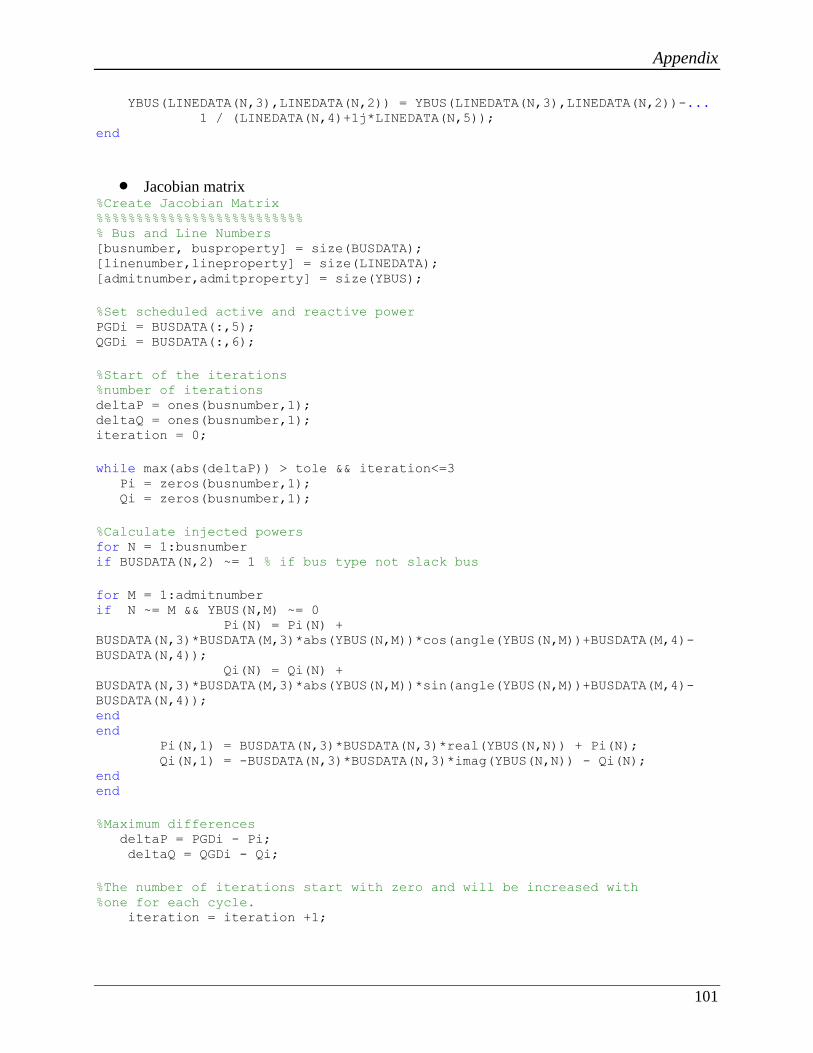
Appendix
101
YBUS(LINEDATA(N,3),LINEDATA(N,2)) = YBUS(LINEDATA(N,3),LINEDATA(N,2))-... 1 / (LINEDATA(N,4)+1j*LINEDATA(N,5)); end
Jacobian matrix %Create Jacobian Matrix %%%%%%%%%%%%%%%%%%%%%%%%%% % Bus and Line Numbers [busnumber, busproperty] = size(BUSDATA); [linenumber,lineproperty] = size(LINEDATA); [admitnumber,admitproperty] = size(YBUS);
%Set scheduled active and reactive power PGDi = BUSDATA(:,5); QGDi = BUSDATA(:,6);
%Start of the iterations %number of iterations deltaP = ones(busnumber,1); deltaQ = ones(busnumber,1); iteration = 0;
while max(abs(deltaP)) > tole && iteration<=3 Pi = zeros(busnumber,1); Qi = zeros(busnumber,1);
%Calculate injected powers for N = 1:busnumber if BUSDATA(N,2) ~= 1 % if bus type not slack bus
for M = 1:admitnumber if N ~= M && YBUS(N,M) ~= 0 Pi(N) = Pi(N) +
BUSDATA(N,3)*BUSDATA(M,3)*abs(YBUS(N,M))*cos(angle(YBUS(N,M))+BUSDATA(M,4)-
BUSDATA(N,4)); Qi(N) = Qi(N) +
BUSDATA(N,3)*BUSDATA(M,3)*abs(YBUS(N,M))*sin(angle(YBUS(N,M))+BUSDATA(M,4)-
BUSDATA(N,4)); end end Pi(N,1) = BUSDATA(N,3)*BUSDATA(N,3)*real(YBUS(N,N)) + Pi(N); Qi(N,1) = -BUSDATA(N,3)*BUSDATA(N,3)*imag(YBUS(N,N)) - Qi(N); end end
%Maximum differences deltaP = PGDi - Pi; deltaQ = QGDi - Qi;
%The number of iterations start with zero and will be increased with %one for each cycle. iteration = iteration +1;
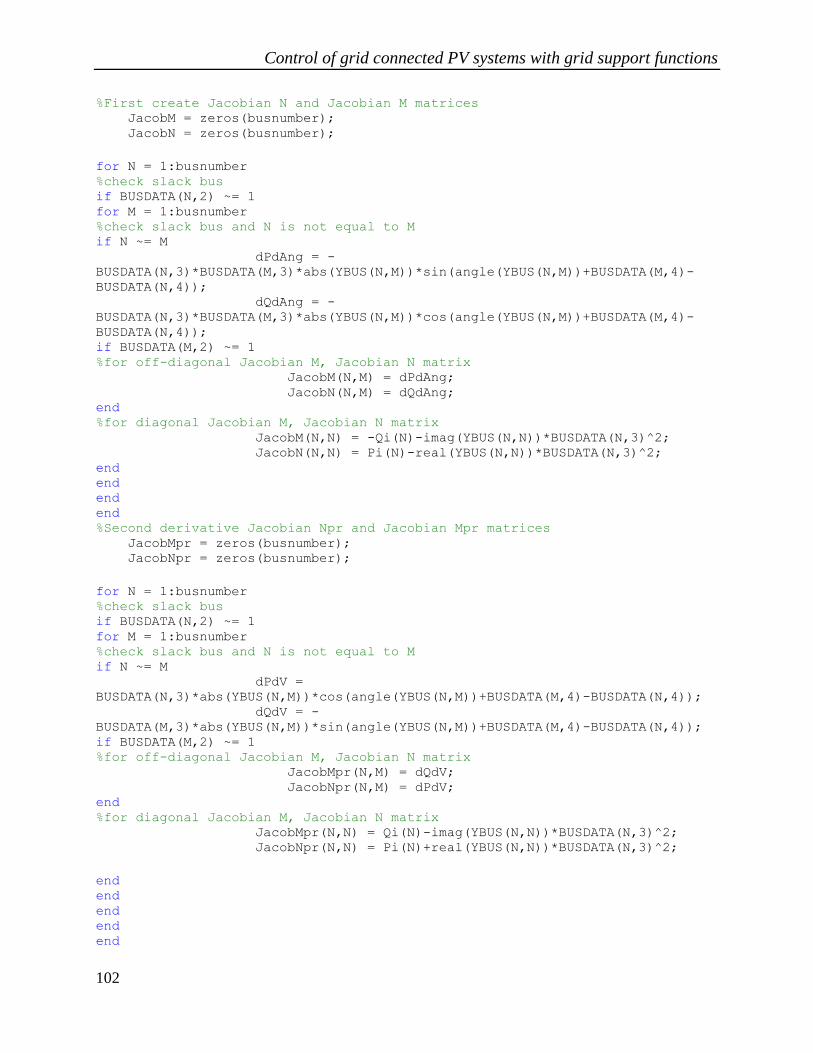
Control of grid connected PV systems with grid support functions
102
%First create Jacobian N and Jacobian M matrices JacobM = zeros(busnumber); JacobN = zeros(busnumber);
for N = 1:busnumber %check slack bus if BUSDATA(N,2) ~= 1 for M = 1:busnumber %check slack bus and N is not equal to M if N ~= M dPdAng = -
BUSDATA(N,3)*BUSDATA(M,3)*abs(YBUS(N,M))*sin(angle(YBUS(N,M))+BUSDATA(M,4)-
BUSDATA(N,4)); dQdAng = -
BUSDATA(N,3)*BUSDATA(M,3)*abs(YBUS(N,M))*cos(angle(YBUS(N,M))+BUSDATA(M,4)-
BUSDATA(N,4)); if BUSDATA(M,2) ~= 1 %for off-diagonal Jacobian M, Jacobian N matrix JacobM(N,M) = dPdAng; JacobN(N,M) = dQdAng; end %for diagonal Jacobian M, Jacobian N matrix JacobM(N,N) = -Qi(N)-imag(YBUS(N,N))*BUSDATA(N,3)^2; JacobN(N,N) = Pi(N)-real(YBUS(N,N))*BUSDATA(N,3)^2; end end end end %Second derivative Jacobian Npr and Jacobian Mpr matrices JacobMpr = zeros(busnumber); JacobNpr = zeros(busnumber);
for N = 1:busnumber %check slack bus if BUSDATA(N,2) ~= 1 for M = 1:busnumber %check slack bus and N is not equal to M if N ~= M dPdV =
BUSDATA(N,3)*abs(YBUS(N,M))*cos(angle(YBUS(N,M))+BUSDATA(M,4)-BUSDATA(N,4)); dQdV = -
BUSDATA(M,3)*abs(YBUS(N,M))*sin(angle(YBUS(N,M))+BUSDATA(M,4)-BUSDATA(N,4)); if BUSDATA(M,2) ~= 1 %for off-diagonal Jacobian M, Jacobian N matrix JacobMpr(N,M) = dQdV; JacobNpr(N,M) = dPdV; end %for diagonal Jacobian M, Jacobian N matrix JacobMpr(N,N) = Qi(N)-imag(YBUS(N,N))*BUSDATA(N,3)^2; JacobNpr(N,N) = Pi(N)+real(YBUS(N,N))*BUSDATA(N,3)^2;
end end end end end

Appendix
103
tempbusnumber = busnumber;
while tempbusnumber > 0,
% the row and column for Jacobian is cut out if slack bus
if BUSDATA(tempbusnumber,2) == 1 JacobM(tempbusnumber,:) = []; JacobM(:,tempbusnumber) = [];
JacobN(tempbusnumber,:) = []; JacobN(:,tempbusnumber) = [];
JacobMpr(tempbusnumber,:) = []; JacobMpr(:,tempbusnumber) = [];
JacobNpr(tempbusnumber,:) = []; JacobNpr(:,tempbusnumber) = []; deltaP(tempbusnumber,:) = []; deltaQ(tempbusnumber,:) = [];
end tempbusnumber = tempbusnumber-1; end
% construct Jacobian from the 4 matrices
J1 = vertcat(JacobM,JacobN); J2 = vertcat(JacobNpr,JacobMpr); Jacobian = horzcat(J1,J2); deltaPQ = vertcat(deltaP,deltaQ);
deltaAngV = (Jacobian)\deltaPQ;
deltaAng = deltaAngV(1:busnumber-1); deltaV = deltaAngV(busnumber:end);
tempAng = zeros(busnumber,1); tempV = zeros(busnumber,1); delta1 = 1; %counter for deltaAng delta2 = 1; %counter for deltaV
for N = 1:busnumber if BUSDATA(N,2) ~= 1 tempAng(N,1) = deltaAng(delta1,1) + BUSDATA(N,4); delta1 = delta1 + 1;
if BUSDATA(N,2) ~= 1 tempV(N,1) = BUSDATA(N,3)*(deltaV(delta2,1) + 1); delta2 = delta2 + 1; end else tempAng(N,1) = BUSDATA(N,4); tempV(N,1) = BUSDATA(N,3);

Control of grid connected PV systems with grid support functions
104
end end
%Update bus voltage magnitudes and angles BUSDATA(:,3) = tempV; BUSDATA(:,4) = tempAng;
%xlswrite('Results.xlsm',tempV,6,'A1:A19');
%Print iteration results only fprintf('-----Results after iteration %d -----\n', iteration); fprintf('Bus Number V(p.u.) Phase angle (degrees) \n');
for N = 1:busnumber fprintf('%d',N); fprintf(' %6.4f',BUSDATA(N,3)); fprintf(' %6.4f\n',BUSDATA(N,4)*deg); end
Objective function
function y = QFunction_correct(x,PG, G, B, BUSDATA) % LINE LOSSES FUNCTION
[busnumber, busproperty] = size(BUSDATA); G1 = zeros(1,busnumber); G2 = zeros(1,busnumber);
y = sum(power(x(2*busnumber+2:end),2));
Contraints function [c, ceq] = Constraints(x,PG,S,BUSDATA, V2) %NONLINEARCONSTRAINT Summary of this function goes here
[busnumber, busproperty] = size(BUSDATA); H = zeros(1,busnumber); H1 = zeros(1,busnumber); H2 = zeros(1,busnumber); H3 = zeros(1,busnumber); H4 = zeros(1,busnumber);
%%%%%%% equality constraints %%%%%%%%%%%%%%% G1 = zeros(1,busnumber); G2 = zeros(1,busnumber);
%%%%% Balanced power equations %%%%% for N = 1:busnumber if BUSDATA(N,2) ~= 1 for M = 1:busnumber if N ~= M && G(N,M) ~= 0 G1(1,N) = G1(1,N)-(x(N)^2*G(N,M)-
x(N)*x(M)*(G(N,M)*cos((x(busnumber+N)-
x(busnumber+M)))+B(N,M)*sin((x(busnumber+N)-x(busnumber+M)))));

Appendix
105
G2(1,N) = G2(1,N)-(-x(N)^2*B(N,M)-
x(N)*x(M)*(G(N,M)*sin((x(busnumber+N)-x(busnumber+M)))-
B(N,M)*cos((x(busnumber+N)-x(busnumber+M))))); end end end G1(1,N) = PG(1,N)-G1(1,N); G2(1,N) = x(2*busnumber+N)-G2(1,N); end
G1(1,1) = 0; G2(1,1) = 0;
G3=x(20); % slack bus angle G4=x(39); % slack bus reactive power reference G5=x(1)-V2; % slack bus voltage magnitude
%%%%%%%%%%%%%%%%%%%%%%%%%%%%%%%%%%%%%%%%%%%%%%%%%%%%%%% %%%%%%%%% inequality constraints %%%%%%%%%%%%%
for N = 1:busnumber if BUSDATA(N,2) ~= 1 H(1,N) = power(PG(1,N),2)+power(x(1,2*busnumber+N),2)-
power(S(1,N),2); H1(1,N) = x(1,N)-1.026; %upper limit for voltage H2(1,N) = 1-x(1,N); %lower limit for voltage H3(1,N) = x(2*busnumber+N); % inverters only inject reactive power H4(1,N) = -x(busnumber+N); % positive angles end end
%%%%%%%%%%%%%%%%%%%%%%%%%%%%%%%%%%%%%%%%%%%%%%%%%
ceq = [G1, G2, G3, G4, G5]; % equality constraints c = [H, H1, H2, H3, H4]; % inequality constraints
end
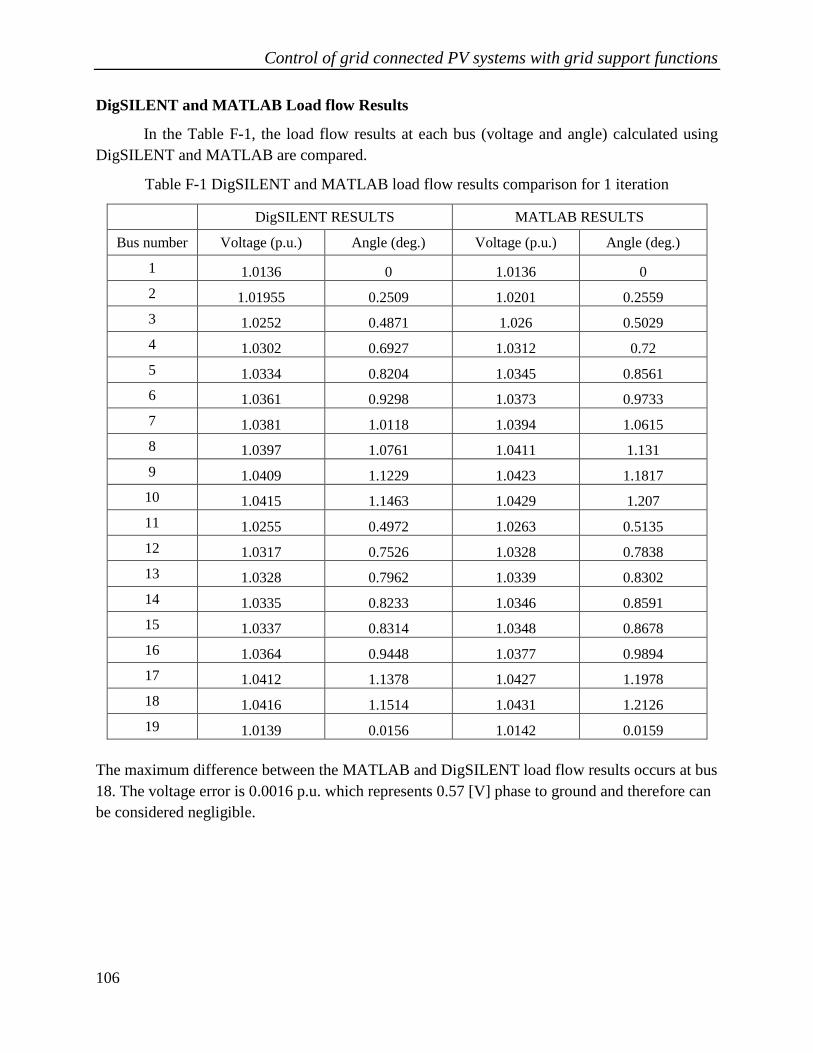
Control of grid connected PV systems with grid support functions
106
DigSILENT and MATLAB Load flow Results
In the Table F-1, the load flow results at each bus (voltage and angle) calculated using
DigSILENT and MATLAB are compared.
Table F-1 DigSILENT and MATLAB load flow results comparison for 1 iteration
DigSILENT RESULTS MATLAB RESULTS
Bus number Voltage (p.u.) Angle (deg.) Voltage (p.u.) Angle (deg.)
1 1.0136 0 1.0136 0
2 1.01955 0.2509 1.0201 0.2559
3 1.0252 0.4871 1.026 0.5029
4 1.0302 0.6927 1.0312 0.72
5 1.0334 0.8204 1.0345 0.8561
6 1.0361 0.9298 1.0373 0.9733
7 1.0381 1.0118 1.0394 1.0615
8 1.0397 1.0761 1.0411 1.131
9 1.0409 1.1229 1.0423 1.1817
10 1.0415 1.1463 1.0429 1.207
11 1.0255 0.4972 1.0263 0.5135
12 1.0317 0.7526 1.0328 0.7838
13 1.0328 0.7962 1.0339 0.8302
14 1.0335 0.8233 1.0346 0.8591
15 1.0337 0.8314 1.0348 0.8678
16 1.0364 0.9448 1.0377 0.9894
17 1.0412 1.1378 1.0427 1.1978
18 1.0416 1.1514 1.0431 1.2126
19 1.0139 0.0156 1.0142 0.0159
The maximum difference between the MATLAB and DigSILENT load flow results occurs at bus
18. The voltage error is 0.0016 p.u. which represents 0.57 [V] phase to ground and therefore can
be considered negligible.

Appendix
107
Appendix G
Source code for the client IEC 61850 application: ****************************************************************************************/ /* ClientMain.c
Includes ***************************************************************************************/ #include <stdio.h> #include <sys/stat.h> //file stat check #include "IEC61850API.h" #include <conio.h> #include <time.h> #include "libxl.h" /* Windows Headers */ #include <windows.h> /****************************************************************************************
Defines ****************************************************************************************/ #define FUNCTION_NAME_LEN 50 float Qref; float Vg_input1=0; float Pset1=0; time_t t; ePrivateObjectType; /****************************************************************************************
Callback function for Update from Server /**************************************************************************************** void UpdateFunction(struct IEC61850_DataAttributeID* ptObjectID_DAID, const IEC61850_ObjectData * ptNewValue) GetConsoleScreenBufferInfo(hOut, &SBInfo); if (ptNewValue->ucType == IEC61850_DATATYPE_FLOAT32) if ((ptObjectID->uiField1==1)&&(ptObjectID->uiField2==2)&&(ptObjectID->uiField3==1)) memcpy(&Vg_input1,ptNewValue->pvData,(ptNewValue->uiBitLength/8)); SetConsoleCursorPosition(hOut,VgRefIs1); printf("%f",Vg_input1); SetConsoleCursorPosition(hOut,SBInfo.dwCursorPosition); if ((ptObjectID->uiField1==1)&&(ptObjectID->uiField2==3)&&(ptObjectID->uiField3==1)) memcpy(&Pset1,ptNewValue->pvData,(ptNewValue->uiBitLength/8)); SetConsoleCursorPosition(hOut,PRefIs1); printf("%f",Pset1); SetConsoleCursorPosition(hOut,SBInfo.dwCursorPosition);

Control of grid connected PV systems with grid support functions
108
/****************************************************************************************
Client Main /**************************************************************************************** int main(void) IEC61850 myClient = NULL; struct IEC61850_Parameters tClientParam; int iError = 0; unsigned char DLL_Loading_Failed=0; printf("\r\n *****************************************************************"); printf("\r\n Client(PC) IEC 61850"); printf("\r\n PED4-1043"); printf("\r\n Vlad Muresan"); printf("\r\n *****************************************************************"); //Load the Client ICD file iError = DLL_IEC61850_LoadSCLFile(myClient,"Client_GSI.ICD"); if(iError != IEC61850_ERROR_NONE) printf("\r\n Error loading Client_GSI.ICD %d. Please refer to API user manual for error message.", iError); SetConsoleCursorPosition(hOut,Position); printf(" "); //clear previous command SetConsoleCursorPosition(hOut,Position); break; //Start the 61850 Client iError = DLL_IEC61850_Start(myClient); if(iError != IEC61850_ERROR_NONE) printf("\r\n Client Start Error %d. Please refer to API user manual for error message.", iError); SetConsoleCursorPosition(hOut,Position); printf(" "); //clear previous command SetConsoleCursorPosition(hOut,Position); break; *********************************************************************************
Main processing loop ********************************************************************************** Sleep(8000); while(1) //char c; IEC61850_ObjectData Value; struct IEC61850_DataAttributeID_Generic Object = 0 ; if (Vg_input1!=0) Qref=(((Vg_input1-230.0)/230.0)*50)*1000; //Droop function memset(&Object,0,sizeof(Object)); Object.uiField1 = 4;

Appendix
109
Object.uiField2=1; Object.uiField3=1; Object.uiField4=0; Object.uiField5=0; Object.Generic_type = IEC61850_DAID_GENERIC; Value.ucType = IEC61850_DATATYPE_FLOAT32; Value.uiBitLength = sizeof(Qref)*8; Value.pvData = &Qref; iError = DLL_IEC61850_Write(myClient, (struct IEC61850_DataAttributeID*)&Object, &Value); if(iError != IEC61850_ERROR_NONE) printf("Failed to write the Qptimal to server ErrorCode:%d. Please refer to API user manual for error message\n.",iError); SetConsoleCursorPosition(hOut,Position); printf(" "); //clear previous command SetConsoleCursorPosition(hOut,Position); else SetConsoleCursorPosition(hOut,QRefIs1); printf("%f",Qref); SetConsoleCursorPosition(hOut,Position); Sleep(63000); /****************************************************************************************
Shutting down client /**************************************************************************************** iError = DLL_IEC61850_Stop(myClient); if(iError != IEC61850_ERROR_NONE) SetConsoleCursorPosition(hOut,ErrorPos); printf("Failed to stop client: %i. Please refer to API user manual for error message.", iError); while(0); if( myClient != NULL ) DLL_IEC61850_Free(myClient); if (hinst_61850DLL) FreeLibrary(hinst_61850DLL); SetConsoleCursorPosition(hOut,ErrorPos); printf("\r\n Application \'SystemCorp 61850 Client\' has terminated. Press Return Key to Exit."); getchar(); return(0); // End main()

Control of grid connected PV systems with grid support functions
110
Source code for the server IEC 61850 application:
/**************************************************************************************** Servermain.c
Includes ***************************************************************************************** #include <stdio.h> #include <sys/stat.h> //file stat check #include <direct.h> //file stat check #include <conio.h> #include <time.h> #include <clib32.h> #include "dSpaceClibInterface.h" #include "IEC61850API.h" typedef struct tag_61850ObjectInt // pointer to IEC61850 object int iObjectValue; /* Object Value */ t61850IntObject; enum VALUE =1, // field 3 description e61850ObjectType; ePrivateObjectType; /* Windows Headers */ #include <windows.h> /****************************************************************************************
Defines ***************************************************************************************** #define FUNCTION_NAME_LEN 50 t61850IntObject INVERTER; int error; int Qset=0; float Vgnew; double Vgnew_double; UInt32 required_size = 500, mem_address; float Vg_input; /****************************************************************************************
Callback functions (read and write from the client) /**************************************************************************************** int myIEC61850_WriteCallback(struct IEC61850_DataAttributeID* ptObjectID_DAID, const IEC61850_ObjectData * ptNewValue) float *float32=NULL; int ErrorCode = IEC61850_CB_ERROR_NONE; switch (ptNewValue->ucType) //The value is updated with the new value

Appendix
111
case IEC61850_DATATYPE_FLOAT32: float32=(float *)ptNewValue->pvData; Vgnew=*float32; if ((ptObjectID->uiField1==4)&&(ptObjectID->uiField2==1)&&(ptObjectID->uiField3==1)) SetConsoleCursorPosition(hOut,QRefIs); printf("%f",Vgnew); SetConsoleCursorPosition(hOut,SetVgPos);
//**************WRITE VALUE TO DSPACE******************************** error = initializedSpace(); //this part starts the board_register part if (error != 0) exit(1); error= initializedSpaceVariables(); //this part starts the functions part if (error != 0) exit(1); Vgnew_double=(double)(Vgnew); if (Vgnew_double!=0) writeParameterValue((double)Vgnew_double, ReactivePowerAddress); error=DS_free_mem(board_index, &mem_address); //******************************************************************************** ErrorCode=IEC61850_CB_ERROR_NONE; break; return ErrorCode; /****************************************************************************************
61850 SERVER MAIN /**************************************************************************************** int main(void) IEC61850 myServer = NULL; double GridVoltageMagnitude, trip, inverter_state, VgRMS, IgRMS, PgRMS, DCVoltage, DCCurrent, ActivePower, ReactivePower, Ref_ActivePower; float Vg=0, Pset=0; ************************************************************************"); printf("\r\n Server (IED) Application IEC 61850"); printf("\r\n PED4-1043"); printf("\r\n Vlad Muresan, IED1 station"); printf("\r\n ************************************************************************"); //Load the Client ICD file iError = DLL_IEC61850_LoadSCLFile(myServer,"Server_GSI.ICD"); if(iError != IEC61850_ERROR_NONE) printf("\r\n Error loading Server_GSI.ICD. %d. Please refer to API user manual for error message.", iError); SetConsoleCursorPosition(hOut,Position); printf(" "); //clear previous command SetConsoleCursorPosition(hOut,Position);

Control of grid connected PV systems with grid support functions
112
break; //Start the 61850 Server iError = DLL_IEC61850_Start(myServer); if(iError != IEC61850_ERROR_NONE) printf("\r\n Server Start Error %d. Please refer to API user manual for error message.", iError); SetConsoleCursorPosition(hOut,Position); printf(" "); //clear previous command SetConsoleCursorPosition(hOut,Position); break; /*****************************************CLIB PART ************************************* // CLIB functions check & start inverter // MEASUREMENTS of signals ***************************************************************************************** error = initializedSpace(); if (error != 0) exit(1); error= initializedSpaceVariables(); if (error != 0) exit(1); writeParameterValue((double)0, ActivePowerAddress); writeParameterValue((double)0, ReactivePowerAddress); error = writePLL(0); error = writePLL(1); printf("\n"); printf("\n"); time(&t); printf("Time %s\n", ctime(&t)); printf("PLL was reset\n"); error = readGrigVoltageMagnitude(&GridVoltageMagnitude); printf("Grid voltage magnitude is %.2f\n", GridVoltageMagnitude); Sleep(500); error = readTripValue(&trip); if (trip==0) printf("Inverter interface problem. Check hardware!\n"); else printf("No trip detected\n"); error = writeInverterReset(1); Sleep(500); error = writeInverterReset(0); printf("Inverter was reset\n"); Sleep(500); error = readInverterStartValue(&inverter_state); if (inverter_state==0) printf("Inverter is OFF. Please start the inverter\n");

Appendix
113
//START INVERTER error = writeInverterStartValue(1); printf("Inverter is ON!\n"); Sleep(500); //WRITE ACTIVE POWER REFERENCE writeParameterValue((double)300, ActivePowerAddress); printf("\n"); //PRINT VALUES FOR ENABLE AND TRIP SetConsoleCursorPosition(hOut,Enab);//enable if (inverter_state==1) printf("ON"); if (inverter_state==0) printf("OFF"); SetConsoleCursorPosition(hOut,SetTrip); if (trip==0) printf("0"); else printf("1"); Sleep(6000); /********************************main processing loop ****************************/ while(x<4) IEC61850_ObjectData Value; struct IEC61850_DataAttributeID_Generic Object = 0 ; SetConsoleCursorPosition(hOut,SetVgRef); SetConsoleCursorPosition(hOut,InputPos); Position.Y=InputPos.Y; //MEASUREMENTS FROM DSPACE error = readParameterValue(&VgRMS, GridVoltageAddress); error = readParameterValue(&IgRMS, GridCurrentAddress); SetConsoleCursorPosition(hOut,IgPos);//Pref printf("%lf", IgRMS); error = readParameterValue(&PgRMS, GridPowerAddress); error = readParameterValue(&DCVoltage, DCVoltageAddress); SetConsoleCursorPosition(hOut,VdcRefIs);//Pref printf("%lf", DCVoltage); error = readParameterValue(&DCCurrent, DCCurrentAddress);

Control of grid connected PV systems with grid support functions
114
SetConsoleCursorPosition(hOut,IdcRefIs);//Pref printf("%lf", DCCurrent); error = readParameterValue(&ActivePower, ActivePowerAddress); error = readParameterValue(&ReactivePower, ReactivePowerAddress); Sleep(500); Vg=(float)(VgRMS); if (Vg!=0) SetConsoleCursorPosition(hOut,Position); memset(&Object,0,sizeof(Object)); Object.uiField1 = 1; Object.uiField2=2; Object.uiField3=1; Object.uiField4=0; Object.uiField5=0; Object.Generic_type = IEC61850_DAID_GENERIC; Value.ucType = IEC61850_DATATYPE_FLOAT32; Value.uiBitLength = sizeof(Vg)*8; Value.pvData = &Vg; //write to the control iError = DLL_IEC61850_Update(myServer, (struct IEC61850_DataAttributeID*)&Object, &Value); if(iError != IEC61850_ERROR_NONE) SetConsoleCursorPosition(hOut,ErrorPos); printf("Failed to write the grid voltage ErrorCode:%d. Please refer to API user manual for error message.",iError); SetConsoleCursorPosition(hOut,Position); else SetConsoleCursorPosition(hOut,VgPos); printf("%f",Vg); SetConsoleCursorPosition(hOut,Position); if (Vg!=0) SetConsoleCursorPosition(hOut,Position); Pset=(float)(ActivePower); memset(&Object,0,sizeof(Object)); Object.uiField1 = 1; Object.uiField2=3; Object.uiField3=1; Object.uiField4=0; Object.uiField5=0; Object.Generic_type = IEC61850_DAID_GENERIC; Value.ucType = IEC61850_DATATYPE_FLOAT32; Value.uiBitLength = sizeof(Pset)*8; Value.pvData = &Pset; //write to the control iError = DLL_IEC61850_Update(myServer, (struct IEC61850_DataAttributeID*)&Object, &Value);

Appendix
115
if(iError != IEC61850_ERROR_NONE) SetConsoleCursorPosition(hOut,ErrorPos); printf("Failed to write the grid voltage ErrorCode:%d. Please refer to API user manual for error message.",iError); SetConsoleCursorPosition(hOut,Position); else SetConsoleCursorPosition(hOut,PRefIs); printf("%f",Pset); SetConsoleCursorPosition(hOut,Position); else//exit SetConsoleCursorPosition(hOut,ErrorPos); printf("Voltage magnitude is not in the prescribed limits 0.85Vg.....1.15Vg ",iError); _getch(); break; x++; Sleep(20000); /*********************************************************************************
Shutting down client ********************************************************************************** iError = DLL_IEC61850_Stop(myServer); error = writeInverterStartValue(0); //stop the inverter if(iError != IEC61850_ERROR_NONE) SetConsoleCursorPosition(hOut,ErrorPos); printf("Failed to stop client: %i. Please refer to API user manual for error message.", iError); while(0); if( myServer != NULL ) // End of program DLL_IEC61850_Free(myServer); if (hinst_61850DLL) FreeLibrary(hinst_61850DLL); SetConsoleCursorPosition(hOut,ErrorPos); printf("\r\n Application \'SystemCorp 61850 Server\' has terminated. Press Return Key to Exit."); return(0);

Control of grid connected PV systems with grid support functions
116
Appendix H
Validation plots of IEC 61850 Client/Server Application
This section presents the complete experimentally validation plots for the client/server
application from Chapter 5, section 5.3. Each simulated iteration is shown.
I. Iteration 1
Figure H-1 Iteration 1, Station 1 server console application and Control Desk

Appendix
117
Figure H-2 Iteration 1, Station 2 server console application and Control Desk

Control of grid connected PV systems with grid support functions
118
Figure H-3 Iteration 1, Station 3 server console application and Control Desk

Appendix
119
Figure H-4 Iteration 1, Client console applications
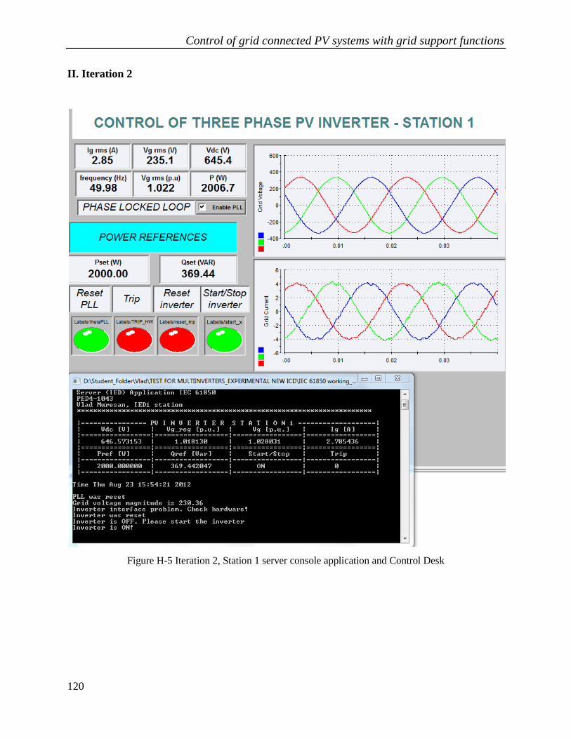
Control of grid connected PV systems with grid support functions
120
II. Iteration 2
Figure H-5 Iteration 2, Station 1 server console application and Control Desk
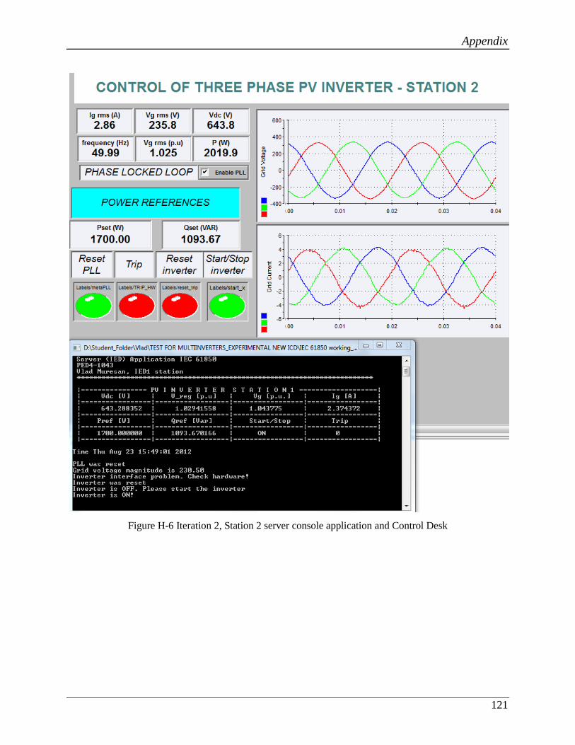
Appendix
121
Figure H-6 Iteration 2, Station 2 server console application and Control Desk

Control of grid connected PV systems with grid support functions
122
Figure H-7 Iteration 2, Station 3 server console application and Control Desk

Appendix
123
Figure H-8 Iteration 2, Client console applications

Control of grid connected PV systems with grid support functions
124
III. Iteration 3
Figure H-9 Iteration 3, Station 1 server console application and Control Desk

Appendix
125
Figure H-10 Iteration 3, Station 2 server console application and Control Desk

Control of grid connected PV systems with grid support functions
126
Figure H-11 Iteration 3, Station 3 server console application and Control Desk

Appendix
127
Figure H-12 Iteration 3, Client console applications

Control of grid connected PV systems with grid support functions
128
IV. Iteration 4
Figure H-13 Iteration 4, Station 1 server console application and Control Desk

Appendix
129
Figure H-14 Iteration 4, Station 2 server console application and Control Desk

Control of grid connected PV systems with grid support functions
130
Figure H-15 Iteration 4, Station 3 server console application and Control Desk

Appendix
131
Figure H-16 Iteration 4, Client console applications

Control of grid connected PV systems with grid support functions
132
Appendix I - Publication
B.I.Craciun, D.Sera, E.A.Man, V.Muresan, T. Kerekes, R.Teodorescu
Improved Voltage Regulation Strategies by PV Inverters in LV Rural Networks;
Power Electronics for Distributed Generation Systems (PEDG) 2012, Page(s) 775-781.

Improved Voltage Regulation Strategies by PV Inverters in LV Rural Networks
Bogdan-Ionut Craciun Department of Energy Technology
Aalborg University Pontoppidanstraede 101 9220 Aalborg, Denmark
Dezso Sera Department of Energy Technology
Aalborg University Pontoppidanstraede 101 9220 Aalborg, Denmark
Elena Anamaria Man Department of Energy Technology
Aalborg University Pontoppidanstraede 101 9220 Aalborg, Denmark [email protected]
Tamas Kerekes Department of Energy Technology
Aalborg University Pontoppidanstraede 101 9220 Aalborg, Denmark
Vlad Alexandru Muresan Department of Energy Technology
Aalborg University Pontoppidanstraede 101 9220 Aalborg, Denmark
Remus Teodorescu Department of Energy Technology
Aalborg University Pontoppidanstraede 101 9220 Aalborg, Denmark
Abstract—The growth of world energy demand and the environmental concerns lead to an increase of renewable energy production over the last decade. The increased number of grid-connected photovoltaic (PV) systems gave rise to problems concerning the stability and safety of the utility grid, as well as power quality issues. Lately, PV generators are required, according to the new German Grid Code (GC), to contribute to the grid stability and to provide grid classical functions during normal and abnormal operation. The purpose of this article is to investigate and optimize the standard voltage regulation methods for low voltage (LV) grid-connected PV systems. Reactive power supply strategy proposed by the German GC Q(U) is investigated and simulated performing load flow analysis on a European residential network benchmark. In order to improve the reactive power transfer in the system, an optimized algorithm of voltage regulation is designed with the aim of minimizing the losses in the system for a better integration of PV power generation into the grid.
I. INTRODUCTION Over the last decade various reasons have determined a
continuous increase of the PV power systems. Some of them are the price drop of PV modules manufacturing, better social acceptance of PV parks or government support for renewable energy [1].
According to European Photovoltaic Industry Association (EPIA), at the end of 2011 the total installed PV capacity in the world has reached over 67.4 GW, with an increase of 68.5 % comparable to 2010. Europe still leads the market with over 50 GW of cumulative power installed with a 70 % increase in 2011. Italy became for the first time the top PV market in 2011 with 9 GW of newly connected capacity, with an impressive 290% increase from 2010 [2]. This increase was a consequence of advantageous tariffs if the systems were installed by the end of 2010 and connected until mid 2011. Germany was the second big player on the
PV market in 2011 with 7.5 GW of new connected systems with a 44% increase from 2010 where more than 80% of the installed systems were located in the LV network [2, 3].
The fast expansion of PV system into the lower parts of the grid raised several concerns for grid reinforcement. In consequence, grid operators had to impose strict operational rules in order to keep the LV grid under control and to harmonize the behavior of all distributed generators connected to it in terms of reliability, efficiency and costs [4][5].
The first cost-effective measure, which brought a major improvement to the grid stability, was for the grid operators to suggest PV systems manufacturers to equip their products with grid support functions [6]. It is expected that until the end of 2015, the shipments of smart inverters in terms of MW will have a market share of 60 %, overtaking the standard inverter. Still, most of them will have only reactive power capabilities [7].
Fig. 1Total world market share for standard and smart PV inverters [7]
80
MW
ship
men
ts (%
of t
otal
)
70
60
50
40
30
20
10
0
90
2010 2011 2012 2013 2014 2015
Standard inverter
Smart inverter
3rd IEEE International Symposium on Power Electronics for Distributed Generation Systems (PEDG) 2012
978-1-4673-2023-8/12/$31.00/ ©2012 IEEE 775
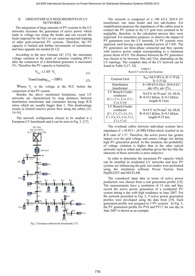
II. GRID INTERFACE REQUIREMENTS IN LV NETWORKS
The integration of large amounts of PV systems to the LV networks increases the generation of active power which leads to voltage rise along the feeder and can exceed the limits imposed by the GCs or can cause unexpected tripping of other grid-connected PV systems. Therefore, the PV capacity is limited and further investments of transformer and lines upgrade are needed [8-12].
According to the new German GC [13], the maximum voltage variation at the point of common coupling (PCC) after the connection of a distributed generator is maximum 3%. Therefore the PV capacity is limited by:
pcc nV 1.03 V (1)
maxTransf.loading 100% (2)
Where: nV is the voltage at the PCC before the connection of the PV system.
Besides the above mentioned limitations, rural LV networks are characterized by long distances between distribution transformer and consumers having large R/X ratios which are usually bigger than 1. This disadvantage results in limited reactive power flow along the cables [12, 14-16].
The network configuration chosen to be studied is a European LV benchmark and it can be seen in Fig. 2. [17].
Fig. 2 European subnetwork benchmark [17]
The network is composed of a 100 kVA 20/0.4 kV transformer, one main feeder and two sub-feeders. For simplification purposes the impedances of the cables used to connect the PV system to the LV grid were assumed to be negligible, therefore, in the calculation process they were neglected. For simulation purposes, to observe the impact of PV generators over the LV network, 18 PV systems were analyzed, each having a peak installed power of 5 kW. The PV generators are three-phase connected and they operate with reactive power output corresponding to a minimum power factor of 0.9. The distance between the PV generators was chosen to be between 30m and 35m, depending on the LV topology. The complete data of the LV network can be found in Table I [17, 18].
TABLE I Rural LV network specifications
External Grid SSK=84.9 MVA; R=3.79 Ω; X=3.53 Ω
Distribution transformer
S=100 kVA Dy5; 20/0.4 kV; ukr=4%; urr=2%;
LV Branch Feeder conductor
(C11, C15, C16, C17, C18, C19)
NAYY 4x70 mm2 AL OLH; R=0.413 Ω/km; X=0.3 Ω/km;
length=0.3 km;
LV Branch Feeder conductor
(C1, C2, C3, C4, C5, C7, C8, C9, C10, C12,
C13, C14)
NAYY 4x70 mm2 AL OLH; R=0.413 Ω/km; X=0.3 Ω/km;
length=0.35 km;
The overhead cables between individual systems have impedance (0.413 0.300) /kmZ j which resulted in an R/X ratio of 1.37. Therefore, the active power has greater impact over the grid voltage and causes voltage rise during high PV generation period. In this situation, the probability of voltage violation is higher than in the other typical networks such as urban and suburban given the fact that the character of those networks is more inductive.
In order to determine the maximum PV capacity which can be installed in residential LV networks and how PV systems are influencing the grid, test studies were performed using the simulation software Power Factory from DigSILENT and MATLAB.
The considered input data in terms of active power production was chosen from a real generation profile [19]. The measurements have a resolution of 15 min and they record the active power generation of a residential PV system during a day with high irradiance in June 2007. For the network presented in Fig. 2, 9 active power generation profiles were developed using the data from [19]. Each generation profile was assigned to 2 PV systems. In Fig. 3, the PV generation profile for PV8 and PV17 for one day in June 2007 is shown as an example.
MV GridSsk=84.9 MVA
R=3.79Ω , X=3.53Ω
R1
R2
R19
PV19PV2
R3PV3
R11
PV11
R4R12 R13 R14 R15
PV12 PV13 PV14 PV15
PV4
R5
PV5
R7 R8 R9 R17
PV8
PV17
R6
PV16
R16
PV6 PV7
PV9
R10R18
PV18
C19 C1
C2
C11
C16
C3
C4
C5
C12 C13 C14 C15
PV10
C7 C8 C9 C17
C10
C18
20/0.4 kV
3rd IEEE International Symposium on Power Electronics for Distributed Generation Systems (PEDG) 2012
776

Fig. 3 PV8 & PV 17 power generation profile June 2007 [19]
In order to mitigate the voltage rise problem on the chosen LV network, successive load flow calculations are performed. The bus where the low-voltage side of the transformer is connected (R1) was chosen to be the slack bus and the PV generators are modeled as PQ sources. The initial conditions for the load flow calculation are: voltage magnitude pcc
iV 1 p.u. and angle i 0 . These conditions refer to all the buses in the network (slack and PQ buses).To emphasize the voltage increase due to PV power generation, a study case with zero load demand was considered.
First load flow analysis must be performed with the following conditions: maximum active power generation and no reactive power consumption. The purpose of this study is to examine the maximum voltage levels in the network and, based on these values, a reactive power compensation strategy can be proposed.
In this case, taking PV17 as an example, it can be observed from Fig. 4 the voltage rise at node R17 is violating the 3% threshold stated in the German standard.
Fig. 4 Voltage profile for PV17 connected to node R17 when no
voltage regulation methods are applied
In order for the whole system to be inbounded under the 3% voltage limit and to avoid power curtailment, PV generators have to adopt voltage regulation methods.
III. VOLTAGE REGULATION METHODS To overcome the voltage variation problem with
minimum reinforcement of the grid, the system operators recently adopted new GCs [13, 20] which require from PV generators to be more flexible and to provide voltage regulation techniques. For this purpose, different methods are proposed with the focus on static droop characteristics. The main voltage regulation methods are the following:
Power factor characteristic: cosφ (P) method Fixed power factor: cosφ method Fixed reactive power: Q method Reactive power /voltage characteristic: Q(U)
The fixed cosφ and Q methods assign a corresponding power factor respectively reactive power reference for the PV generators based on the network power flow investigation. Load power profile information and PV power production are needed in order to assign a reasonable fixed reactive power set values to the inverters. Studies have shown that fixed cosφ and Q methods are not suitable for the LV networks due to their incapability of maintaining the voltage within limits and unnecessary reactive power consumption/absorption [9, 14, 18].
The cosφ (P) method is calculating the reactive power reference depending on the active power generation of the PVs. When the power generation value reaches half of the PV nominal power, the power factor decreases towards 0.9 and reactive power is absorbed based on a cosφ (P) droop characteristic. This method does not use the grid voltage information and is only assuming that high power generation matches the voltage increase [18].
The Q(U) strategy calculates the reactive power reference for each PV system depending on the voltage magnitude at the corresponding PCC. Therefore, the PV systems situated at the end of the feeder will start absorbing reactive power earlier than the PV systems located near the transformer. Moreover, the voltage magnitude at the buses near the transformer is likely to be within prescribed limits; hence they will not participate in the regulation process, making the task more difficult for the other PV systems.
The aim of this paper is to optimize the Q(U) regulation algorithm in terms of using the available capacity of all the PV inverters in the regulation process and avoid stressing the ones at the end of the feeder. This optimization strategy can be implemented on a centralized controller which could gather the information from all the PV systems and based on the voltage values it can calculate the optimal reactive power reference for each PV system.
The focus of the optimized Q(U) algorithm is to:
Maintain the voltages at the PCCs below the specified limit
Minimize the reactive power absorption of the overall network, hence minimize the losses in the line
A. Q(U) method As stated in the German GC [13], the droop curve for
the Q(U) method is provided by the network operator. Therefore, a droop characteristic specific for the network studied in this article must be designed. Based on the results of the first load flow analysis, for the maximum voltage value, the corresponding maximum reactive power absorption value can be assigned. As it can be seen from Fig. 4, this value can be taken as 1.05 p.u. because when there is no reactive power absorption in the network, the
3rd IEEE International Symposium on Power Electronics for Distributed Generation Systems (PEDG) 2012
777

voltage magnitude does not exceed 1.05 p.u.. The start value for absorbing reactive power is chosen to be 1.02 p.u.. Using these values, the droop characteristic can be achieved and the Q(U) regulation method can be implemented (Fig. 5) [18].
Q [kVar]
1
-Qmax
Q [kVar]
Closer to the transformer
PV19 PV181.02 1.05
V [p.u.]0.980.95
Qmax
V [p.u.]2 3 4 17V1 V2 V3 V4
Fig. 5 Static droop curve for Q(U) method
Where 1 2 3V ,V ,V and 4V are the defined voltage values 0.95, 0.98, 1.02, 1.05p.u. and measV is the measured voltage.
The flowchart presented in Fig. 6 the implementation of the Q(U) method. For this purpose the DigSilent Power Factory software was used and for each iteration, two load flow analysis are performed. First, the effect of active power generation on the voltage magnitude is investigated. Based on the measurement, an individual reactive power is assigned to each PV and a new load flow analysis is performed in order to check if the problem has been suppressed.
Start
Assign new value Pi+1
YES
AssignPi value
Calculateload flow
Read bus voltages
Is V3<Vmeas<V4?
AssignQi = 0
NO
Calculatevoltage
deviation
Calculate Q reference
Calculateload flow
Read bus voltages
Is V3<Vmeas<V4?
YES Is Last iteration?
NO
YESStop
AssignQi = Qmax
Calculateload flow
NO
Read bus voltages
Assign new
value Pi+1
Fig. 6 Load flow simulation algorithm for Q(U) method
The algorithm for Q(U) method can be summarized by the script from (3). It can be mentioned that for the LV network studied in this article, the only concern is the voltage rise problem and PV systems are required only to absorb reactive power, therefore only the corresponding part from the Q(U) scrip was considered for implementation.
max
max
max
max
meas 1
meas 11 meas 2
1
2 meas 3
meas 33 meas 4
3
Q ; V V
V V100 Q ; V V V
V
Q 0; V < V V
V V100 ( Q ; V V V
V
Q ;
)
meas 4 V V>
(3)
B. Optimized Q(U) algorithm Nomenclature:
bN - total number of buses in the system
PQN - number of PQ buses in the system
iV - voltage magnitude at bus i ref refi iP ,Q - active and reactive power injected at bus i
iS - rated power of PV inverters
ij ijG ,B - mutual conductance and susceptance between bus i and j
ii iiG ,B - self conductance and susceptance of bus i
ij - voltage angle difference between bus i and j
The optimization problem treated in this subchapter refers to the reactive power dispatch problem. The optimization algorithm has a specific objective function to be minimized while satisfying some predefined equality and inequality constraints.
The objective of this algorithm is to calculate an optimal value for the reactive power reference of each PV inverter. In this way, all the inverters will participate in the voltage regulation process with an optimized percent of their available reactive power capacity. [21]
In order to achieve this objective, it is necessary to properly adjust some variables like voltage magnitude and angle in each node. The equality constraints are formed by the power flow equations while the inequality constraints are the limits on voltage magnitude at PCCs and the inverter capacity.
The objective function of the algorithm can be expressed as the sum of all the reactive power references of the PV systems:
bN 2ref
ii 2
F Q
(4)
The equality constraints are represented by the power flow equations:
bNrefi i j ij ij ij ij b
j 1P V V (G cos B sin ) 0,i N 1
(5)
bNrefi i j ij ij ij ij PQ
j 1Q V V (G cos B sin ) 0,i N
(6)
3rd IEEE International Symposium on Power Electronics for Distributed Generation Systems (PEDG) 2012
778

The inequality constraints are the following:
Voltage limit at PCC:
pcci n bV 1.03V ,i N (7)
Inverter capacity:
2 2ref ref 2i i i bP Q S ,i N 1
(8)
The first step consists of performing a load flow analysis with the given initial conditions and afterwards, the optimized Q(U) algorithm takes the calculated values and performs the optimization. The variables in the system are the reactive power reference ( ref
iQ = 0) as control variable and two state variables: voltage magnitude ( pcc
iV ) and angles ( i ). Taking into consideration the equality and inequality constrains, a feasible solution will be obtained. The new values will be given as reference to the inverters and another load flow analysis will be performed in order to check if the voltage is kept between limits.
C. Study case results The performance of the above described methods is
investigated based on the reactive power flow and voltage level.
The main difference between the two strategies is the fact that while for the first one, each PV inverter absorbs a calculated value of reactive power corresponding to its local voltage magnitude, for the second strategy, the amount of reactive power values are computed based on all the PCC voltages of the network. In consequence, the optimized Q(U) algorithm makes the LV network more flexible in terms of connecting more PV systems.
In the first case, the behavior of the PV3 system was investigated. Knowing that the system is closer to the transformer, there was no overvoltage problem at the corresponding PCC, as seen from Fig. 7.
Fig. 7 Voltage profile at the PCC3 for the analyzed strategies
However, taking into consideration the droop characteristic of the Q(U) strategy, the PV3 inverter will start absorbing reactive power when the voltage at PCC3 exceeds the value 1.02 p.u.. As seen from Fig. 8, the value of the reactive power absorbed using the optimized Q(U) method is lower.
Fig. 8 Reactive power consumption of PV generator at the PCC3
Even though the voltage level using the optimized Q(U) method are higher compared to the voltage using the Q(U) algorithm, the benefit of the optimized method is the minimization of the reactive power absorption while the PV generators maintain their operation in maximum power point tracking.
Taking PV17 as a second example, from Fig. 9 it can be noticed that the voltage at PCC17 exceeds the 1.03 limit if no reactive power compensation methods are available.
Fig. 9 Voltage profile at the PCC17 for the analyzed strategies
In Fig. 10, the reactive power absorption of PV17 inverter is shown and, as expected, when using the Q(U) method, higher values of reactive power are necessary to be absorbed compared to the values when using the optimized Q(U) strategy.
Fig. 10 Reactive power consumption of PV generator at the PCC17
3rd IEEE International Symposium on Power Electronics for Distributed Generation Systems (PEDG) 2012
779

Fig. 11 and Fig. 12 presents the total active and reactive power losses before and after performing the Q(U) optimized algorithm.
Fig. 11 Total active power losses in the network
Fig. 12 Total reactive power losses in the network
Besides the optimization of the reactive power reference, the proposed algorithm presents the benefit of minimizing the active and reactive power line losses. This is achieved because the load flow equations are taken as equality constraints and the optimization algorithm performs the balancing of the power transfer in the network.
In Fig. 13, the transformer loading for the Q(U) method is presented. As it can be seen, the transformer does not exceed 100% loading.
Fig. 13 Transformer loading for Q(U) method
Due to the fact that the optimized Q(U) method is absorbing less reactive power than the Q(U) method, it can
be stated that the transformer does not exceed the 100% loading in this case also. In addition, the optimized Q(U) method presents the advantage of less stressing the transformer.
IV. CONCLUSIONS This paper focuses on voltage regulation methods for PV
systems with ancillary services. One of the strategies encouraged in the German GC for LV, the Q(U) strategy, was implemented and simulated on an European LV benchmark grid. Results showed that this regulation method can keep the voltages at PCCs below the 3% limit but with the drawback of absorbing more reactive power than needed. This is because each PV inverter calculates the necessary compensatory reactive power depending on the voltage at the corresponding PCC and based on a Q-U droop characteristic.
An optimized Q(U) algorithm using a centralized controller which is able to dispatch the minimum amount of reactive power to each PV inverter has the purpose to improve the existent solution encouraged by the system operators. The method considers all the voltages at the PCC of each grid-connected PV system in the network and calculates the minimum absorption of reactive power. To develop such optimized control strategy, communication infrastructure is needed in order for the central controller to transmit the calculated values of reactive power for each PV inverter which participates in the voltage regulation process.
The benefits of implementing the optimized Q(U) algorithm are: a better usage of the PV inverter capacity which leads to increased PV capacity in the network, lower transformer loading and lower network losses.
ACKNOWLEDGMENT The authors would like to express their appreciation for
PhD fellow Erhan Demirok and Ass.Prof. Henrik C. Pedersen for their cooperation and professional support.
REFERENCES [1] European Photovoltaic Industry Association, "Market Outlook 2010," 2011. [2] European Photovoltaic Industry Association, "Market Report 2011," 2012. [3] European Photovoltaic Industry Association, "Solar generation 6. solar photovoltaic electricity empowering the world," 2011. [4] K. Budenbender, M. Braun, T. Stetz and P. Strauss, "Multifunctional PV systems offering additional functionalities and improving grid integration," vol. Volume 7, Number 2 (2011) Pages 109-128, 2011. [5] ABB, "IEC 61850: Special report," 2010. [6] A. Mohd, E. Ortjohann, A. Schmelter, N. Hamsic and D. Morton, "Challenges in integrating distributed energy storage systems into future smart grid," in Industrial Electronics, 2008. ISIE 2008. IEEE International Symposium on, 2008, pp. 1627-1632. [7] IMS Research Organization, "The World Market for PV Inverters 2011 Report," 2011. [8] G. Kerber, R. Witzmann and H. Sappl, "Voltage limitation by autonomous reactive power control of grid connected photovoltaic inverters," in Compatibility and Power Electronics, 2009. CPE '09. 2009, pp. 129-133. [9] E. Demirok, P. Casado González, K. H. B. Frederiksen, D. Sera, P. Rodriguez and R. Teodorescu, "Local Reactive Power Control Methods for Overvoltage Prevention of Distributed Solar Inverters in Low-Voltage Grids," Photovoltaics, IEEE Journal of, vol. 1, pp. 174-182, 2011.
3rd IEEE International Symposium on Power Electronics for Distributed Generation Systems (PEDG) 2012
780

[10] A. Canova, L. Giaccone, F. Spertino and M. Tartaglia, "Electrical impact of photovoltaic plant in distributed network," in Industry Applications Conference, 2007. 42nd IAS Annual Meeting. Conference Record of the 2007 IEEE, 2007, pp. 1450-1455. [11] N. Grass, G. Kerber, R. Witzmann, M. Sebeck and R. Keck, "Increasing Grid Transmission Capacity and Power Quality by new Solar Inverter Concept and Inbuilt Data Communication," Telecommunication - Energy Special Conference (TELESCON), 2009 4th International Conference on, pp. 1-5, 2009. [12] L. Herman, B. Blazic and I. Papic, "Voltage profile support in LV distribution networks with distributed generation," in Universities Power Engineering Conference (UPEC), 2009 Proceedings of the 44th International, 2009, pp. 1-5. [13] VDE, "Generators connected to the low-voltage distribution network-Technical requirements for the connection to and parallel operation with low-voltage distribution networks (VDE-AR-N 4105)," 2011. [14] T. Stetz, W. Yan and W. Braun, "Voltage Control in distribution systems with high level PV penetration (Improving absorption capacity for PV systems by reactive power supply);" vol. 25th European PV Solar Energy Con-ference and Exhibition, 6th - 10th September 2010, Valencia, Spain, 2010. [15] E. Demirok, D. Sera, R. Teodorescu, P. Rodriguez and U. Borup, "Clustered PV inverters in LV networks: An overview of impacts and comparison of voltage control strategies," in Electrical Power & Energy Conference (EPEC), 2009 IEEE, 2009, pp. 1-6. [16] G. Kerber, "Statistiche analyse von NS-VErteilungsnetzen und modellierung von referenznetzen," 2208. [17] Cigre Task Force C6.04.02, "Benchmark Systems for Network Integration of Renewable and Distributed Energy Resources," 2011. [18] M. Braun, T. Stetz, T. Reimann, B. Valov and G. Arnold, "Optimal reactive power supply in distribution networks; Technological and economic assessment for PV systems," vol. 24th European Photovoltaic Solar Energy Conference and Exhibition, Hamburg, 2009. [19] D. EnergiMidt Entreprise A/S, "The SOL-300 project – A 300 roof-top project," 1998-2001. [20] BDEW - Bundesverband der Energie- und Wasserwirtschaft, "Generating Plants Connected to the Medium-Voltage Network, Technical Guideline," 2008. [21] L. Soder, "Load flow study and sensitivity analysis of power systems,"EG2030 Power System - advanced course, Sweden
3rd IEEE International Symposium on Power Electronics for Distributed Generation Systems (PEDG) 2012
781