DEPARTMENT OF ECONOMICS YALE UNIVERSITY

P.O. Box 208268 New Haven, CT 06520-8268

http://www.econ.yale.edu/

Economics Department Working Paper No. 36

Cowles Foundation Discussion Paper No. 1638

Do Local Economic Development Programs Work? Evidence from the Federal Empowerment Zone Program

Matias Busso and Patrick Kline

February 2008

This paper can be downloaded without charge from the Social Science Research Network Electronic Paper Collection:

http://ssrn.com/abstract=1090838

Do Local Economic Development Programs Work?

Evidence from the Federal Empowerment Zone Program∗

Matias Busso

University of Michigan

matiasb@umich.edu

Patrick Kline

Yale University

patrick.kline@yale.edu

Abstract

This paper evaluates the impact of Round I of the federal urban EmpowermentZone (EZ) program on neighborhood level labor and housing market outcomes over theperiod 1994-2000. Using four decades of Census data in conjunction with informationon the proposed boundaries of rejected EZs, we find that neighborhoods receivingEZ designation experienced substantial improvements in labor market conditions andmoderate increases in rents relative to rejected and future zones. These effects wereaccompanied by small changes in the demographic composition of the neighborhoods,though evidence from disaggregate Census tabulations suggests that these changesaccount for little of the observed improvements.

First version: April 18, 2006

This version: November 28, 2007

JEL Codes: H2, O1, R58, C21.

∗The authors would like to thank Soren Anderson, Timothy Bartik, John Bound, Charlie Brown, KerwinCharles, John DiNardo, Taryn Dinkelman, Jesse Gregory, Jim Hines, Ben Keys, Justin McCrary, Gary Solon,Joel Slemrod, and Jeff Smith for encouragement and advice on this project. We would also like to thankparticipants of the University of Michigan Labor Seminar, the Michigan Public Finance Brownbag Lunch,and the Upjohn Institute Seminar for useful comments. This work has been supported (in part) by a grantfrom the National Poverty Center at the University of Michigan. Any opinions expressed are those of theauthors.

Local economic development programs are an important, yet understudied, feature of

the U.S. tax and expenditure system. Timothy Bartik (2002) estimates that state and lo-

cal governments spend $20-30 billion per year on economic development programs with an

additional $6 billion per annum coming from the federal government. However, little acad-

emic work has been done examining the impact of these expenditures on local communities,

largely because of the small scale and general diversity of most such programs.1 This paper

evaluates the federal urban Empowerment Zone (EZ) program, which constitutes one of the

largest standardized federal interventions in impoverished urban American neighborhoods

since President Johnson’s Model Cities program.

With a mandate to revitalize distressed urban communities, the EZ program represents a

nexus between social welfare policy and economic development efforts. Unlike conventional

anti-poverty programs, Empowerment Zones aim to help the poor by subsidizing demand

for their services at local firms, which has made them one of the few social welfare programs

popular on both sides of the congressional aisle. In an era where non-entitlement spending

on social welfare programs has been scaled back dramatically, the federal Empowerment

Zone program has enjoyed rapid growth. After the initial funding of six first round EZs and

two “supplemental” EZs in 1994, fifteen more cities were awarded zones in 1999, followed

by another eight in 2001. An additional forty-nine urban areas were concurrently granted

smaller Enterprise Communities (ECs) which entailed a reduced package of benefits. The

enthusiasm for spatially targeted tax credits has led to the birth of a variety of new zones,

each modifying the original EZ concept in different ways.2 Most recently, the justification for

tax abatement zones has been expanded to include disaster relief. For example, in the wake

of the September 11th attacks, parts of New York city were designated “Liberty Zones”

and granted a variety of localized tax credits; while, in 2006, Congress passed legislation

authorizing a set of “Gulf Opportunity Zones” for areas stricken by Hurricane Katrina.

These recent forays of the IRS into the business of local economic development should

merit the attention of economists. The GAO (1999) estimates that the first round Empow-

erment Zones will cost $2.5 billion over the course of the ten year program. Given that EZ

neighborhoods have a total population of under a million people, subsidies of this magnitude,

when directed to such relatively small urban areas, might be expected to have important

effects upon the behavior of firms and workers. Measuring the nature and magnitude of these

1See Bartik (1991) and the volume by Nolan and Wong (2004) for a review.2In addition to urban EZs and ECs, there are a series of rural EZs and ECs, Enhanced Enterprise Commu-nities (EECs), and 28 urban and 12 rural “Renewal Communities” entitled to benefits similar in magnitudeto EZs.

2

behavioral responses is crucial for understanding the equity-efficiency tradeoffs inherent in

geographically targeted transfers.3

The EZ program was pre-dated by a series of state initiated “enterprise zones” which

varied dramatically in scale, purpose, and implementation.4 A modest literature evaluating

the state level programs reaches mixed conclusions reflecting, in part, the enormous diversity

of the programs under examination.5 Some programs only provide for investment subsidies

while others include employment tax credits; some state zones cover hundreds of square

miles, while others are focused on particular neighborhoods within a few cities. Besides

differences in the structure of the programs themselves, a number of methodological problems

hinder clear interpretation of the enterprise zone literature. Many of the early studies faced

difficulties obtaining data corresponding to the boundaries of the state zones, relying instead

upon evaluations at higher levels of aggregation such as the zip code or city which likely

reduced the statistical power of the estimates. Furthermore, most studies rely upon simple

variants of the differences in differences research design without examining in any detail the

suitability of the control groups being used to proxy the counterfactual behavior of the zones

(a notable exception being Boarnet and Bogart (1996)). Finally, all of the studies of which

we are aware save for Papke (1994) calculate standard errors ignoring issues of spatial and

temporal dependence in the data making it difficult to assess exactly how precise previous

studies have been and whether the differences in results are attributable to chance.

The federal EZ program is much larger in scope and scale than its state level precursors

and involves a standardized package of fiscal benefits applied to neighborhoods defined in

terms of 1990 census tracts. Unlike most state level zones, the EZ program ties business tax

credits to the employment of local residents and includes a series of large block grants aimed

at reducing poverty and improving local infrastructure. The only large scale study of the

impact of EZ designation is an interim evaluation (Hebert et al., 2001) performed for HUD

by Abt Associates in conjunction with the Urban Institute, which finds that EZs had large

effects on job creation, with increases in local payrolls on the order of 10%.

The Abt study suffers from a number of important weaknesses. First, it relies upon within

city comparisons of census tracts which are likely to overstate the effect of the program if

EZ designation merely reallocates jobs between neighborhoods. Second, the matching algo-

rithm used to find controls for the EZ tracts is poorly documented and standard errors are

3See Nichols and Zeckhauser (1982) for an introduction to the economics of targeting.4See Papke (1993) and Hebert et al. (2001) for a history of the Empowerment and Enterprise Zone ideas.5See Papke (1993, 1994), Boarnet and Bogart (1996), Bondonio (2003), Bondonio and Engberg (2000),Elvery (2003), and Engberg and Greenbaum (1999). Peters and Peters and Fisher (2002) provide a review.

3

not provided making it difficult to draw strong conclusions regarding the results. Moreover,

important questions exist about the quality and representativeness of the Dunn and Brad-

street data used in the analysis.6 Third, since local governments designed Empowerment

Zone boundaries, it is possible that census tracts awarded EZs would have improved relative

to other tracts in the same city even in the absence of EZ designation if the boundaries

were drawn based upon trends emerging at the beginning of the 1990s. Finally, the study

provides no guidance as to whether the jobs being created in EZs were staffed by local resi-

dents, whether the neighborhood composition of EZ residents changed, and whether poverty,

unemployment, or the local housing market responded to the treatment–questions that are

key to evaluating the success or failure of the program.

This paper uses four decades of census data on local neighborhoods in conjunction with

proprietary EZ application data obtained from HUD to assess the impact of Round I EZ

designation on residential sorting behavior and local labor and housing market outcomes over

the period 1994-2000.7 Unlike previous studies we use census tracts in rejected and future

Empowerment Zones as controls for first round EZs. Since these tracts were nominated for EZ

designation by their local governments, they are likely to share unobserved traits and trends

in common with first round EZs which also underwent a local nomination phase. We present

an extensive body of evidence indicating that these controls serve as good proxies for the

counterfactual behavior of EZ tracts over the 1990s. Moreover, because most of our control

tracts are in different cities than those winning EZs, they are substantially less susceptible

to contamination by spillover or general equilibrium effects than those of previous studies.

We use a variety of semiparametric methods to adjust for the small observable differences

that do exist between our control tracts and EZs and to increase the statistical power of our

analysis.

We find that neighborhoods receiving EZ designation experienced substantial improve-

ments in the labor market outcomes of zone residents and moderate increases in housing

values and rents relative to observationally equivalent tracts in rejected and future zones.

These effects were accompanied by small changes in the demographic composition of the

neighborhoods. We provide evidence from disaggregate census tabulations that the observed

improvements in the local labor market conditions of EZ neighborhoods are unlikely to have

resulted from these demographic changes alone. Employment rates, for example, seem to

6See Heeringa and Haeussler (1993) and Appendix A of the Abt report.7The outcomes are: poverty, employment, unemployment, owner occupied housing values, rents, meanearnings, population, the fraction of houses that are vacant, the fraction of the neighborhood that is black,the fraction of residents who live in the same house as five years ago, and the fraction of residents who holda college degree.

4

have increased even among young high school dropouts. However, given the high rates of

turnover in EZ neighborhoods we cannot determine whether the benefits of EZ designation

were captured by pre-existing residents or new arrivals with similar demographic character-

istics.

An impact analysis is performed indicating that the EZ program created approximately

$1 billion of additional wage and salary earnings in EZ neighborhoods and another $1 billion

in property wealth. A comparison of IRS data with our impact estimates suggests that the

tax credits associated with EZ designation are unlikely to have been the only source of the

observed employment gains. Rather, we conclude that the block grants and outside funds

leveraged by EZ designation, perhaps in conjunction with changes in expectations associated

with EZ status, are likely to have contributed substantially to the changes in the local labor

market.

The remainder of the paper is structured as follows: Section I provides background on

the EZ program, Section II discusses the expected impact of EZ benefits, and Section III

describes the data used. Section IV introduces the identification strategy and details the

methodology used, Section V discusses results and tests for violations of the assumptions

underlying our identification strategy. Section VI provides an impact analysis and Section

VII concludes.

I. A Crash Course in Empowerment

The federal Empowerment Zone program is a series of spatially targeted tax incentives

and block grants designed to encourage economic, physical, and social investment in the

neediest urban and rural areas in the United States. Talk of a federal program caught

on early in President Clinton’s first term following the 1992 Los Angeles riots. In 1993,

Congress authorized the creation of a series of Empowerment Zones and smaller Enterprise

Communities (ECs) that were to be administered by the Department of Housing and Urban

Development (HUD) and awarded via a competitive application process.

Communities were invited to create their own plans for an EZ and submit them to HUD

for consideration. Plans included the boundaries of the proposed zone, how community

development funds would be used, and how state and local governments and community or-

ganizations would take actions to complement the federal assistance. In addition to providing

a guidebook to communities hoping to apply, HUD held a series of regional workshops to ex-

plain the EZ initiative and the requisite application process. Nominating local governments

were required to draw up EZ boundaries in terms of census tracts, list key demographic

5

characteristics of each proposed tract including the 1990 poverty rate as measured in the

Decennial Census, and specify whether the tracts were contiguous or located in the central

business district.8

HUD initially awarded EZs to six urban communities: Atlanta, Baltimore, Chicago,

Detroit, New York City, and Philadelphia/Camden. Two additional cities, Los Angeles

and Cleveland, received “supplemental” EZ (SEZ) designation but were awarded full EZ

designation two years later. Forty-nine rejected cities were awarded ECs. Table 1 shows

summary statistics of EZ neighborhoods by city. The average Round I EZ spanned 10.6

square miles, contained 117,399 people, and had a 1990 poverty rate of 45%. Most zones

are contiguous groupings of census tracts, although some EZs, such as the one in Chicago

pictured in Figure 1, cover multiple disjoint groupings of tracts.

EZ designation brought with it a host of fiscal and procedural benefits, which we briefly

summarize here:9

1. Employment Tax Credits —Starting in 1994, firms operating in the six original EZsbecame eligible for a credit of up to 20 percent of the first $15,000 in wages earnedin that year by each employee who lived and worked in the community.10 Tax creditsfor each such employee were available to a business for as long as ten years, withthe maximum annual credit per employee declining over time. This was a substantialsubsidy given that, in 1990, the average EZ worker only earned approximately $16,000in wage and salary income.

2. Title XX Social Services Block Grant (SSBG) Funds —Each EZ became eligible for$100 million in SSBG funds, while each SEZ was eligible for $3 million in SSBG funds.These funds could be used for such purposes as: training programs, youth services,promotion of home ownership, and emergency housing assistance.

3. Section 108 Loan Guarantees/Economic Development Initiative (EDI) Grants —EDIfunds are large flexible grants which are meant to be used in conjunction with othersources of HUD funding to facilitate large scale physical development projects. Thetwo SEZ’s, Los Angeles and Cleveland, received EDI grants of $125 and $87 millionrespectively. The six original EZs were not eligible for these grants. Section 108 LoanGuarantees allow local governments to obtain loans for economic development projects.Los Angeles received $325 million in 108 loan guarantees and Cleveland received $87million.

8For example, the application asked “Does any tract that includes the central business district have a povertyrate of less than 35%?” and “Do all census tracts of the nominated zone have 20% or more poverty rate?”9See IRS (2004) for more details.

10Firms located in the two supplemental Empowerment Zones did not become eligible for the tax credit until1999.

6

4. Enterprise Zone Facility Bonds —State and local governments can issue tax-exemptbonds to provide loans to qualified businesses to finance certain property. A businesscannot receive more than $3 million in bond financing per zone or $20 million acrossall zones nationwide.

5. Increased Section 179 Expensing —Section 179 of the Internal Revenue Code provideswrite-offs for depreciable, tangible property owned by businesses in designated zones.Qualified target area business taxpayers could write off $20,000 more than the usualfirst-year maximum (which in 1994 was $18,000).

6. Regulatory Waivers/Priority in Other Federal Programs —Qualified EZ/EC areas weregiven priority in other Federal assistance programs. Furthermore, as part of theirapplications, EZ/EC applicants were encouraged to request any waivers in Federalprogram requirements or restrictions that were felt to be necessary for the successfulimplementation of their local revitalization strategy.

The subsidies available to zone businesses increased substantially over the first four years

of the program with the surprise introduction of two additional wage credits (the Work

Opportunity Tax credit and the Welfare to Work Tax Credit),11 an expansion of the EZ

Facility Bonds program, and changes in the treatment of capital gains realized from the sale

of EZ assets. By all accounts, the degree of potential fiscal intervention in EZ neighborhoods

was substantial.12

Nevertheless, it is difficult to assess exactly how extensive participation in the program

has been. GAO (1999) estimated that the EZ program would cost $2.5 billion over its

ten year life with 95 percent of the costs coming from the employment credit.13 IRS data

show that, in the year 2000, close to five hundred corporations, and over five thousand

individuals, claimed EZ Employment Credits worth a total of approximately $23.5 and $22

million, respectively.14 Roughly $200 million in employment credits were claimed over the

period 1994 to 2000, with the amount claimed each year trending up steadily over time.

So despite the slow ratcheting up of participation, reasonably large tax subsidies have been

11Work Opportunity Tax Credits enabled businesses to claim up to $2,400 per worker in tax credits for firstyear wages paid to qualifying employees such as ex-felons, and youth ages 18-24 who are zone residents.Welfare to Work Tax Credits allow businesses to claim credits for up to $3,500 of first year and $5,000 ofsecond year wages paid to workers who are long-term recipients of family assistance.12While the SSBG and EDI funds were fungible, the wage credits and capital write offs were relativelynarrowly targeted. Wages paid to workers employed for less than ninety days or relatives were not eligiblefor the wage credits nor were payments to unofficial workers not on the payroll. Similarly, for a businessto be eligible for the tax exempt bond financing or the increased Section 179 expensing it must be able todemonstrate that the majority of its income is earned within the zone and that 35% of its employees arezone residents.13The EZ program has subsequently been extended to expire in 2009.14These figures come from GAO (2004).

7

dispensed to EZ neighborhoods in the form of wage subsidies. In contrast, only 17 EZ facility

bonds were issued before 2000 totalling approximately $50 million, so the impact of the tax

exempt bond financing is probably minimal.

Survey data provide information about who participated in the tax incentives and why.

A 1997 survey of zone businesses conducted by HUD found that most firms were unaware of

the existence of the EZ program, that only 11% claimed to be using the wage tax credit, and

only 4% claimed to be using the Section 179 deductions.15 Such figures mask heterogeneity

in participation rates by firm size. The HUD survey found that large firms used the tax

credits more intensively with 63% and 30% utilization rates for the wage subsidies and

capital write-offs respectively.16 Another survey conducted by the GAO (1999) found that

55% of large urban businesses using the employment credits were manufacturing firms. The

most commonly cited reasons for not using the wage credits were that firms were either

unaware of the benefits or did not qualify for them because their employees lived outside

of the zone. However, even among large firms, 27% responded that they were not aware of

the credit. The low rates of participation in the Section 179 write-off program were most

often attributed to lack of knowledge about the program and ineligibility due to lack of

profits or qualifying investments. Since tax credits can only be claimed against a company’s

taxable profits, many small firms (15%), appear to have been unable to take advantage of

the program due to insufficient taxable income.

Although the tax benefits accompanying EZ designation were somewhat underutilized by

firms, the General Accounting Office (2004) estimates that state agencies had drawn down

approximately 60% of Round I SSBG funds by 2003 and were on target to fully expend

their allocations by the expiration of the program in 2010. More difficult to measure is the

degree of outside investment leveraged by EZ designation. While the first round EZs were

allocated roughly $800 million dollars in SSBG and EDI funds, the annual reports of the

various EZs suggest that massive amounts of outside capital have accompanied the grant

spending. HUD (2003) claims that $12 billion in public and private investment have been

raised from Federal “seed” money accompanying the broader EZ/EC program. Our own

analysis of HUD data suggests that the amount spent on first round EZs over the period

1994-2000 is substantially less than this, but still much greater than the initial amount of

block grant funding allocated.

Table 2 summarizes information from HUD’s internal performance monitoring system

15These figures come from Hebert et al. (2001).16See tables 3-13, 3-14 and 3-15 in Hebert et al. (2001). The sample sizes used in the survey are not largeenough to make strong inferences regarding the relationship between size and participation.

8

on the amount of money spent on various program activities by source. Audits by HUD’s

Office of Inspector General17 and the GAO (2006)18 have called the accuracy of these data

into question, so the figures reported should be interpreted with caution. The six original

EZs reported spending roughly $2 billion by 2000, with more than four dollars of outside

money accompanying every dollar of SSBG funds. The most commonly reported use of funds

was enhancing access to capital. One-stop capital shops providing loans to EZ businesses

and entrepreneurs were a component of the plans of most EZs. In Detroit, a consortium of

lenders provided $1.2 billion to be used in a local loan pool. Although these funds are listed

as being spent, it is difficult to know what fraction were actually loaned out. Analysis of

the HUD data in Hebert et al. (2001) indicates that the total size of all loan pools across

the six original EZs was only $79 million. The second most common use of the funds was

business development which included technical and financial assistance. Third and fourth

most common respectively were expenditures on housing development and public safety.

Compiling the tax and expenditure information together and allowing for biases in the

reporting behavior of EZs, we estimate that the EZ program resulted in expenditures over the

period 1994-2000 of between one and three billion dollars. While this amount of expenditure

is below what was originally envisaged at the inception of the program, it is still quite

substantial considering that together the EZs constitute a 92 square mile area containing

less than a million residents.

II. Expected Impact

The benefits accompanying EZ designation might be expected to impact a number of features

of local communities.19 Here we consider the aggregate variables most likely to respond to

the treatment and the economic interpretation of those responses.

The wage subsidies should have two effects on local labor markets, both militating towards

increased employment of zone residents. First, there should be a scale effect in that the

average cost of labor should fall and production should expand. Second, there should be

a substitution effect as outside workers are replaced by cheaper zone workers. If outside

workers are relatively unwilling to relocate to EZ neighborhoods and zone residents vary

17See Chouteau (1999) and Wolfe (2003).18While the GAO could not find suitable documentation corroborating the dollar amount spent on each pro-gram, they were able to verify HUD data on the number of activities undertaken. Their analysis of this dataindicated that “community development” projects which include “workforce development, human services,education, and assistance to businesses” accounted for more than 50 percent of the activities implementedin the 6 original urban EZs.19See Papke (1993) for a general equilibrium model of the effects of localized tax incentives.

9

substantially in their disutility of work, then we might expect any employment increases to

be accompanied by corresponding increases in local wages.

If firms are only willing to hire the most qualified workers from a neighborhood, then

employment gains need not be accompanied by reductions in poverty as the relatively high

skilled workers will merely shift from one job to another. Likewise, if EZ neighborhoods

lack residents with the sorts of skills desired by firms then the wage subsidies may not be

successful in increasing neighborhood employment as firms will not find it profitable to hire

unproductive workers even at a substantial discount.

To the extent that block grants and other subsidies increase the profitability of local busi-

nesses, such as by alleviating capital constraints, providing technical assistance, or reducing

crime, a scale effect should ensue, leading to an increase in the number of jobs inside EZs.20

Moreover, if, as suggested by HUD’s administrative data, a substantial portion of funds are

being invested in workforce development and the matching of workers to local employers, we

should expect local employment of zone residents to increase. Funds spent on improvement

of infrastructure and physical redevelopment might also be expected to temporarily increase

local employment in the form of construction jobs.

Housing markets should respond in tandem with zone labor markets. Firms and resi-

dential developers21 may bid up the price of zone land in pursuit of EZ benefits if those

benefits are deemed valuable. Likewise, block grants and outside investments in physical

development and community safety are likely to improve the amenities associated with EZs,

possibly stimulating residential demand in the area.22 The asset values of land and owner

occupied housing may rise quickly if expectations of future market conditions are influenced

by EZ designation and there are obstacles in the short run to increasing housing supply.

Rental rates, by contrast, will reflect supply and demand conditions in the spot market for

housing. However if zone amenities improve, or if outside workers seek to migrate to the

zone in anticipation of future neighborhood improvements, quality adjusted rents will rise.23

20Reductions in the price of capital should also bring with them a substitution effect as capital is substitutedfor labor. In theory this effect could outweigh the scale effect and yield negative employment effects ifcapital and low skilled labor are gross substitutes. We consider such extreme cases implausible. However,the substitutability of capital and low-skill labor may be expected to result in fairly small net impacts onemployment.21EDI and SSBG funds are targeted towards the development of affordable housing and the promotion ofhome ownership. In practice, these funds, in conjunction with the Low-Income Housing Tax Credit, areoften spent in public-private physical development projects.22According to Hebert et al. (2001) the majority of EZ businesses reported in 2000 that neighborhoodconditions were “much improved” or “somewhat improved” since 1997.23In some of the zone cities rents are regulated meaning that housing will be rationed.

10

Over longer time horizons the supply of housing may increase or the quality of the housing

stock may adjust, both of which should moderate any price effects.

Since most zone residents are renters, large increases in rents may lead to gentrification

and neighborhood churning as more affluent newcomers displace prior zone residents. To the

extent that gentrification does occur, it should be reflected in changes in the demographic

composition of zone neighborhoods. Increases in the price of land might also be expected

to bring with them reductions in the fraction of units in a neighborhood that are vacant.

However, local landlords may postpone the sale of vacant units to developers if property

values are expected to rise faster than the interest rate. Therefore the expected impact of

EZ designation on the fraction of units vacant is ambiguous.

III. Data

To perform the analysis we constructed a detailed panel dataset combining information from

the Decennial Census, the County/City Databook, and HUD. The primary data source

utilized is the Neighborhood Change Database (NCDB) which is a panel of census tracts

spanning the period 1970-2000 constructed by Geolytics and the Urban Institute. Appendix

I provides more detailed information about this dataset and how it was constructed. Tract

level Decennial Census information from the NCDB was merged with relevant editions of the

County/City Databook to yield a hierarchical longitudinal dataset with four decades worth

of information on cities and tracts.24

In order to construct a suitable control group for EZs, we obtained 73 of the 78 first round

EZ applications submitted to HUD by nominating jurisdictions via a Freedom of Information

Act request.25 These applications contain the tract composition of rejected zones, along with

information regarding the number of political stakeholders involved in each proposed zone.26

We merged this information with data from HUD’s web site detailing the tract composition

of future zones to create a composite set of rejected and future zones to serve as controls for

EZs in our empirical work. Appendix Table A1 details the composition of the cities in our

evaluation sample, whether they applied for a Round I EZ, and the treatments (if any) they

received.

24Tracts that crossed city boundaries were assigned to the city containing the highest fraction of theirpopulation.25The scoring information is not in the public domain and was not released to us by HUD.26Since the applications proposed EZs in terms of 1990 census tracts and the NCDB uses 2000 census tractdefinitions we use the Census Tract Relationship Files of the U.S. Census Bureau to map the former intothe latter.

11

IV. Methodology

A. Identification Strategy

The credibility of any non-experimental evaluation hinges critically upon the nature of the

treatment assignment mechanism. In order to receive EZ designation, tracts had to pass two

stages of selection. First, they had to be nominated by local officials for inclusion in an EZ.

Second, the EZ proposal of which they were a part had to be chosen by HUD. While little is

known about the initial nomination process, HUD’s decision making process has been fairly

well documented. EZ applications were ranked and scored according to their ability to meet

four criteria: economic opportunity, community-based partnership, sustainable community

development, and a strategic vision for change. Explicit eligibility criteria specified mini-

mum rates of poverty and unemployment and maximum population thresholds for groups of

proposed census tracts as measured in the 1990 Census.27 The authorizing legislation also

reserved designations for nominees with certain characteristics.28 Scores were assigned to

each application by an interagency review team consisting of approximately 90 individuals.

HUD’s Department of Community Planning and Development oversaw the review team. Af-

ter the HUD committee submitted its scores and recommendations the selection decisions

were made by HUD Secretary Cisneros in consultation with a 26 member oversight orga-

nization known as the Community Empowerment Board. The CEB was chaired by Vice

President Gore and staffed by cabinet secretaries and other high ranking officials. After des-

ignations were made the CEB was used to coordinate support for EZs and ECs from other

agencies.

Following allegations of impropriety in the popular press an investigation was conducted

by the HUD inspector general finding some irregularities in the scoring process including

that some of the lower ranked EC applications were considered for awards.29 However, the

audit indicated that all six of the first round EZs were chosen from a list of 22 applications

designated as “strong” by the HUD selection committee. Wallace (2003) analyzes the assign-

ment process, finding that political variables are poor predictors of EZ designation. Rather,

27All zone tracts were required to have poverty rates above twenty percent. Moreover, ninety percent of zonetracts were required to have poverty rates of at least twenty-five percent and fifty percent were required tohave poverty rates of at least thirty-five percent. Tract unemployment rates were required to exceed 6.3%.The maximum population allowed within a zone was 200,000 or the greater of 50,000 or ten percent of thepopulation of the most populous city within the nominated area.28For example one urban EZ had to be located in an area where the most populous city contained 500,000or fewer people. Another EZ was required to be in an area that included two states and had a combinedpopulation of 50,000 or less.29See Greer (1995). Secretary Cisneros informed the inspector general’s office that “he used the [HUD]staff’s general input, as well as his personal knowledge and perspectives on individual community needs,commitment and leadership, in making the final designations and award decisions.”

12

variables such as community participation, size of the empowerment zone, and poverty were

the best predictors of receipt of treatment.

We will compare the experience over the 1990s of Round I EZs to tracts in rejected and

later round zones with similar historical Census characteristics.30 Since much of the data

used by HUD to select zones came from the 1990 Census it seems reasonable to believe that

rejected and future zones with similar census covariates can serve as suitable controls for

winning zones. We present a variety of evidence including a series of “false experiments”

suggesting that this is indeed the case. Because some of the control zones used in this

approach received treatment in the form of ECs, we expect that the resulting estimates of

the impact of EZ designation will be biased towards zero, making our estimates relatively

conservative.31

Since the majority of rejected and future zones are located in different cities than treated

zones, we are able to assess the sensitivity of our estimates to geographic spillover effects.

This is an important advantage of our work over the Abt study (and many of the studies of

state level enterprise zones) which relied entirely upon within city comparisons. Two sorts of

local spillovers are plausible. First, some of the “leveraged” outside funds flowing to EZs may

have been diverted from other impoverished neighborhoods in the same cities or metropolitan

areas. Such reallocations would serve to exaggerate the impact of EZ designation found

by a within-city estimator since the control tracts would actually be receiving a negative

treatment. Second, any true impact of EZ designation on labor or housing market conditions

in EZ neighborhoods may spillover into adjacent neighborhoods. This could bias a within

city estimator in the opposite direction, though the expected sign depends upon the outcome

in question and the underlying economic parameters governing the process.32 Without prior

information on the size of these two spillover effects, one cannot know which effect will

dominate or the composite direction of bias.

Though the use of rejected tracts as controls has many advantages, one may still be

concerned that the cities that won first round EZs are fundamentally different from losing

30Use of rejected applicants as controls as a means of mitigating selection biases has a long history in theliterature on econometric evaluation of employment and training programs. See the monograph by Bell etal. (1995) for a review.31ECs did not receive wage tax benefits but were allocated $3 million in SSBG funds and made eligible fortax exempt bond financing. As mentioned earlier, the bond financing does not appear to have been heavilyutilized.32Though one would normally expect improvements in the amenity value of one neighborhood to yield housingprice increases in both that neighborhood and adjacent neighborhoods, it is possible, if neighborhoods aregross substitutes, for the prices of adjacent neighborhoods to be negatively correlated. Similarly, it is possiblefor job growth inside of EZs to occur at the expense of neighborhoods outside of EZs if firms merely relocatebetween neighborhoods without expanding total employment.

13

cities. A cursory inspection of Table 1 indicates that the three largest US cities all won EZs,

while the remaining winners are large manufacturing intensive cities. If large cities experi-

enced fundamentally different conditions over the 1990s than small cities, the comparison

of observationally equivalent census tracts in winning and losing zones will be biased. To

further explore this possibility we construct a set of “placebo zones” in each city receiving

an EZ. Each placebo zone contains the same number of census tracts as the actual EZ in

that city and possesses similar demographic characteristics. We compare the experience of

these placebo zones over the 1990s to that of the rejected and later round zones and find no

appreciable differences, bolstering our confidence in the credibility of our findings.

B. Econometric Model

Let outcomes in application tract i in city c in decade t be represented by Yict.33 Suppose

that these outcomes are generated by a model of the form:

Yict = µt (Dict, Yict−1, Xict−1, Zct−1, ηct, εict) + θi (1)

where µt (.) is some function indexed by time, Dict is a treatment dummy, Yict−1 is the tract

outcome lagged, Xict−1 is a vector of predetermined tract characteristics, Zct−1 is a vector of

predetermined city wide characteristics, θi is a tract fixed effect, ηct is a random city specific

year shock, and εict is a serially correlated tract specific error term which is assumed to be

independent of all other right-hand-side variables.

The class of stochastic processes encompassed by (1) is capable of capturing many of the

key features one would expect to see in a panel of census tracts. It allows for mean reverting

tract and city specific shocks and for conditional correlation of outcomes across tracts within

a city and within tracts across time. Moreover, substantial heterogeneity across tracts is

permitted, both in their mean outcomes and in their potential responses to EZ designation.

It will be convenient to reexpress the dependence of the function µt (Dict, .) on EZ des-

ignation by writing µt (Dict, .) = Dictµ1t (.) + (1−Dict) µ0

t (.). The (contemporaneous) effect

of EZ designation on outcomes in a given tract may now be defined as βi = µ1t (.) − µ0

t (.).

Note that this effect is a potentially nonlinear function of the predetermined covariates

Yict−1, Xict−1, and Zct−1. This reflects the notion that neighborhoods with different degrees

of pre-existing economic distress are likely to exhibit different responses to EZ designation.

33From this point on we use the phrase “application tract” interchangeably with “proposed tract” to referto application and future EZ tracts.

14

In order to eliminate the tract fixed effect θi, let us rewrite (1) in first differences using

the potential outcomes notation of Neyman (1923) and Rubin (1974):

∆Y 1ict = βi + ht (Ωit, Uict) (2)

∆Y 0ict = ht (Ωit, Uict)

where ht (.) = µ0t (.) − µ0

t−1 (.), Ωit = (Yict−1, Xict−1, Zct−1, Yict−2, Xict−2, Zct−2), and Uict =

(ηct, εict, ηct−1, εict−1). Superscripts index potential outcomes under different treatment states.

Because we have only one post-treatment decade in the data we only consider static treat-

ment schemes (i.e. we do not consider potential outcomes associated with two decades of

EZ designation or one decade of designation followed by a decade of nondesignation). Thus,

∆Y 1ict represents the change in Yict a tract would have experienced over the 1990s had it been

awarded an EZ at the beginning of the decade, while ∆Y 0ict represents the change that would

have occurred over the 1990s without an EZ. Because we only observe one of these potential

outcomes per tract we may write ∆Yict = ∆Y 1ictDict + ∆Y 0

ict (1−Dict).

Suppose that application tracts were awarded Empowerment Zone status by HUD based

upon the history of their Census covariates available in 1990 and other random factors. We

model this selection mechanism as Dict = 1 if D∗ict > 0 and 0 otherwise where34

D∗ict = λΩit + vict (3)

λ is a coefficient vector and vict is a random error assumed to be independent of Ωit and

Uict—an assumption we display here for future reference:

vict ⊥ (Ωit, Uict) (4)

In words, this means that conditional on covariates, EZ designation is independent of the

experience a proposed census tract would have had over the 1990s in the absence of treatment.

This assumption directly implies that the distribution of untreated potential tract outcomes

f (∆Y 0ict|Dict, Ωit) is independent of whether or not a tract actually received treatment so that

f (∆Y 0ict|Dict, Ωit) = f (∆Y 0

ict|Ωit). Rosenbaum and Rubin (1983) term this the Conditional

Independence Assumption (CIA) and it forms the cornerstone of our difference-in differences

identification strategy. The CIA has the following important implication:

E[∆Y 0

ict|Ωit, Dict = 0]

= E[∆Y 0

ict|Ωit, Dict = 1]

(5)

34This abstracts from the two step nature of the selection process inherent in EZ assignment. See AppendixII for a justification of the approach taken here.

15

which states that, conditional on covariates, EZ and non-EZ tracts would, on average, be

expected to experience the same changes in outcomes during the 1990s in the absence of

treatment.

Recall that the tract specific impact of EZ designation βi is itself a function of the

covariates. A standard parameter of interest in the program evaluation literature is the

mean effect of treatment on the treated (Heckman and Robb, 1985), which may be defined

as:

TT = E[∆Y 1

ict −∆Y 0ict|Dict = 1

]= E [βi|Dict = 1]

As the name suggests, this concept measures the average impact of the program on those

who take it up, or in this case, those tracts awarded EZ designation. Since EZ tracts have

roughly similar numbers of people, weighting the effect on each tract equally approximates

the national impact on EZ residents.

Estimating TT requires identifying two moments. The first E [∆Y 1ict|Dict = 1] is trivially

identified by the unweighted sample mean of treated observations on ∆Yict. The second

moment, E [∆Y 0ict|Dict = 1] , is the counterfactual mean of the treated observations had they

not been treated—a quantity with no directly observable sample analogue. We use two

approaches to estimating E [∆Y 0ict|Dict = 1].

The first approach suggested by condition (5) is to approximate the function E[∆Y 0ict|Ωit,

Dict = 0] using a parametric model and then to use that model to compute an estimate of

E [∆Y 0ict|Dict = 1] =

∫E [∆Y 0

ict|Ωit, Dict = 0] dF (Ωit|Dict = 1). We do this by fitting a flexi-

ble regression model to the untreated tracts and using the estimated regression coefficients

to impute the counterfactual mean outcomes of each treated tract. The average difference

between imputed counterfactual outcomes and actual values among treated tracts is then

computed as an estimator of TT . This procedure, which can be thought of as a variant of

the classic Blinder (1973) and Oaxaca (1973) approach to decomposing wage distributions,

can be shown to consistently estimate TT given a sufficiently flexible model for E [∆Y 0ict|Ωit]

(see Imbens, Newey, and Ridder, 2007). Thus for each tract we have an estimate of the

tract specific treatment effect βi = ∆Y 1ict−∆Y 0

ict (Ωit) where ∆Y 0ict (Ωit) = E [∆Y 0

ict|Ωit] is the

prediction from a parametric linear regression function. We then estimate TT using:

B-O =1

N1

∑i∈D=1

βi

The second approach is to estimate the counterfactual mean E [∆Y 0ict|Dict = 1] via propen-

16

sity score reweighting.35 The basic idea of the propensity score approach is to reweight the

data in a manner that balances the distribution of covariates across treated and untreated

tracts. This is accomplished by upweighting untreated tracts that “look like” treated tracts

based upon their observables. Once the distribution of covariates is balanced across treat-

ment and control groups a simple comparison of weighted means will, under the assump-

tions made thus far, identify TT . Moreover, the performance of the reweighting estimator

in balancing the distribution of observables across groups can easily be assessed directly by

comparing reweighted covariate moments.

A key assumption necessary for propensity score based approaches to identify TT is,

P (Dict = 1|Ωit) < 1 (6)

This assumption, which is often referred to as the “common support” condition, states that

no value of the covariates can deterministically predict receipt of treatment. The failure of

this condition would present the possibility that some tracts with particular configurations of

covariates would only be capable of being observed in the treated state, thereby preventing

the construction of valid controls. As suggested by Heckman et al. (1998b) and Crump

et al. (2006) we present results where observations with very high estimated propensity

scores are dropped from the sample. This approach safeguards against violations of the

overlap condition in finite samples and can substantially reduce the sampling variance of the

estimator.36

Conditions (4) and (6) in conjunction with the results of Rosenbaum (1987) imply that37

E[∆Y 0

ict|Dict = 1]

= E[ω (Ωit) ∆Y 0

ict|Dict = 0]

(7)

where ω (Ωit) = p(Ωit)1−p(Ωit)

1−ππ

, p (Ωit) = P (Dict = 1|Ωit) , and π = P (Dict = 1). Thus the

covariate distribution of untreated tracts can be made to mimic that of treated tracts by

weighting observations by their conditional odds of treatment p(Ωit)1−p(Ωit)

times the inverse of

their unconditional odds 1−ππ

. Equation (7) simplifies estimation considerably since rather

35Propensity score reweighting was proposed in the survey statistics literature by Horvitz and Thompson(1952) and adapted to causal inference by Rosenbaum (1987). In the economics literature such estimatorshave been used in a cross-sectional context by DiNardo et al. (1996) and extended to the panel setting byAbadie (2005). Recent work by Hirano, Imbens, and Ridder (2003) demonstrates that properly implementedreweighting estimators are asymptotically efficient in the class of semiparametric estimators.36Trimming slightly modifies the estimand to E

[∆Y 1

ict −∆Y 0ict|∆Dict = 1, P (∆Dict = 1|Ωit) < k

]where k

is a scalar constant. As suggested by Crump et al. (2006) we choose k = 0.9 throughout the paper. In mostspecifications this results in the trimming of a very small fraction (approximately 1%) of the sample.37Proofs of conditions (7) and (8) are provided in Appendix III.

17

than estimating a very high dimensional conditional expectation, for which different tun-

ing parameters might be required for different outcomes, one need only estimate a single

propensity score p (Ωit) = P (Dict = 1|Ωit) (Rosenbaum and Rubin, 1983).38 In practice we

estimate p (Ωit) via a logit and π by N1

N1+N0the fraction of treated tracts in the estimation

sample.

A useful corollary of (7) is that:

E [ω (Ωit) |Dict = 0] = 1 (8)

Which merely states that the mean weight among the controls should equal one. We impose

the sample analogue of this adding up condition when calculating our estimates in order to

reflect the theoretical condition in (8).39

Given estimates p (Ωit) and π we estimate E [ω (Ω) ∆Y 0ict|Dict = 0] with its sample ana-

logue1

N0

∑ p (Ωit)

1− p (Ωit)

1− π

π∆Y 0

ict

We then estimate TT by computing the weighted difference-in-difference (WDD):

WDD =1

N1

∑i∈D=1

∆Y 1ict −

1

N0

∑i∈D=0

p (Ωit)

1− p (Ωit)

1− π

π∆Y 0

ict

Consistency follows subject to the usual regularity conditions by an appropriate law of large

numbers.

Throughout the paper we show results from both the Blinder-Oaxaca (B-O) and reweight-

ing approaches.40 We prefer the reweighting based estimates on the grounds that they allow

us to directly assess the suitability of our specification of the propensity score via visual

inspection of covariate balance and simple diagnostics for the logit which are not outcome

specific. It is also easier to check whether the overlap condition is satisfied with the reweight-

ing approach than the B-O approach. On the other hand, a strength of the parametric B-O

38As pointed out by Heckman et al. (1998a), propensity score approaches do not escape the curse of dimen-sionality since the function p (Ωit) is unknown. The effects on asymptotic bias and variance of adjusting forthe propensity score instead of the underlying covariates of which it is a function are ambiguous (see section7 of that paper).39Equation (8) actually provides us with an overidentifying restriction that can be used as a specificationtest on our model. Very large deviations from 1 of the mean estimated weight among untreated tracts are asign of misspecification. In Appendix Table A4 we conduct formal tests of this restriction.40See DiNardo (2002) for a discussion of the reweighting interpretation of Blinder-Oaxaca and Imbens, Newey,and Ridder (2007) for a demonstration of the first order equivalence of the two approaches.

18

approach is that it can reliably estimate treatment effects even in the absence of overlap if

the parametric model upon which it relies is approximately correct.41

C. Inference Procedures

Confidence intervals and p-values for all estimators are obtained via a pairwise block boot-

strapping algorithm described in Appendix IV. This procedure, which is analogous to cluster

robust inference, resamples cities rather than tracts in order to preserve the within city de-

pendence in the data. Because we are interested in evaluating the effect of EZ designation on

a variety of outcomes, we use a sequential multiple testing procedure suggested by Benjamini

and Hochberg (1995) to control the False Discovery Rate (FDR) of our inferences. The False

Discovery Rate is defined as the expected fraction of rejections that are false and is closely

related to the probability of a type I error. Details of the multiple testing procedure, which

is a function of the single hypothesis p-values, are given in Appendix IV. For convenience

we also report single hypothesis confidence intervals and p-values. From this point on, we

shall refer to outcomes as “significant” at a given level of confidence if the estimated p-value

ensures control of the FDR to the specified level. In general, the multiple testing procedure

requires substantially lower p-values for a given level of significance than an equivalent sin-

gle equation test. Failure to reject a single hypothesis in this multiple testing framework is

equivalent to a failure to reject the joint null hypothesis that all of the treatment effects are

zero.

V. Results

A. Characteristics of EZs and Controls

Table 3 shows average characteristics of winning and losing proposed zones before and after

reweighting.42 For our baseline specification we restrict the sample to zones in cities with

population greater than 100,000. While the residents of rejected and future zones are poor

and have high rates of unemployment we see from columns one and four of Table 3 that

41Another advantage implied by the results of Chen, Hong, and Tarozzi (2004) is that the B-O approach,which is a variant of their CEP-GMM estimator, reaches the semiparametric efficiency bound under weakerregularity conditions than propensity score reweighting.42The variables included in the reweighting logits are reported in Appendix V. Our baseline specificationminimizes the Akaike Information Criteria (see Appendix Table A2). City population could not be includedin the conditioning set because it came too close to perfectly predicting EZ receipt. That we cannot mimicthe city population distribution of EZs via reweighting should be apparent from the list of winning cities inTable 1. To examine whether imbalance in city-wide population affects our DD results we try adding a thirdorder polynomial in 1990 city population to our Blinder-Oaxaca estimator and experiment with a variety ofdifferent sample restrictions, each with a different distribution of city size.

19

they are not quite as poor or detached from the labor force as residents of EZ areas. After

reweighting, however, the mean characteristics of the two groups become substantially more

comparable.

Figure 2 shows the time series behavior of the EZ and control tracts with and without

reweighting. When reweighting methods are applied to the pooled set of controls their history

over the past two decades mirrors that of actual Empowerment Zones remarkably well. There

is no dip in outcomes prior to EZ designation of the sort found by Ashenfelter (1978) in

studying training programs and for some outcomes the time series behavior of the treatment

and control groups over the three decades prior to treatment is almost indistinguishable.

One can actually see most of our results from these graphs themselves. The key labor

market variables (employment, unemployment, and poverty) all seem to have improved in EZ

neighborhoods relative to reweighted controls over the 1990s. A few demographic variables

such as the fraction of the population with college degrees also appear to have been impacted

by the program.

Columns two and three of Table 3 indicate that control tracts in treated cities have some-

what different characteristics from those in untreated cities. Moreover, our earlier discussion

of spillover effects suggested that the use of controls in treated cities has the potential to

confound a differences in differences estimator. Table 4 investigates whether pooling control

tracts in treated cities with those in rejected cities is likely to introduce important biases

into our analysis. This is accomplished by applying our difference in differences estimators

to the sample of controls, coding tracts in future EZs in treated cities as the treated group

and all other control tracts as untreated. The first column gives the results of a “naive”

difference-in-differences analysis without covariate adjustments, the second column presents

the results of our preferred reweighted difference-in-differences estimator, the third column

shows the results of the regression based Blinder-Oaxaca estimator, and the fourth column

adds a third order polynomial in city population to the Blinder-Oaxaca model.

From the first column of Table 4 we see that over the 1990s, control tracts in treated

cities experienced smaller increases in the share of residents with college degrees, slightly

lower increases in rents, and a greater increase in the fraction of vacant houses than other

controls. After conditioning on pre-treatment characteristics all of these relationships disap-

pear. In fact, the magnitude of the differential experience of the two sets of controls over the

1990s tends to be very close to zero, though the reweighting estimator finds a rather large

difference in the behavior of mean earnings. This aberrant earnings result disappears in the

Blinder-Oaxaca based estimates. We take this as evidence that the two sets of control tracts

20

are roughly exchangeable conditional on predetermined characteristics. In our subsequent

analysis we pool together the two sets of controls in order to gain power and to improve the

degree of covariate overlap with the EZ tracts.43

B. Baseline Results

Table 5 presents numerical estimates of the impact of EZ designation on EZ neighborhoods.

The naive DD estimator finds a large (29.7%) increase in the value of owner occupied housing,

a 4 percentage point increase in the fraction of the neighborhood that is employed, a 4.1

percentage point decrease in the fraction of the neighborhood that is unemployed, and a 4.9

percentage point decrease in poverty. Reweighting the DD estimator for covariate imbalance

changes the magnitude (though not the sign) of many of the point estimates. The estimated

impact on housing values falls to 22.4 percent, while the impact on rents rises dramatically to

7.7% and becomes statistically significant. The reweighting estimator also finds a significant

2.3 percentage point increase in the fraction of residents with a college degree and a 2.6

percentage point decrease in the fraction of residents that are black. The estimated impacts

on the labor market variables (employment, unemployment, earnings, and poverty) remain

essentially unchanged.

For comparison we also report regression based Blinder-Oaxaca estimates in Column 3.

The Blinder-Oaxaca method yields point estimates similar to those found by the reweighting

estimator though the statistical precision of the estimates sometimes differs. It finds smaller

(though still significant) effects of EZ designation on housing values, rents, poverty, unem-

ployment, and employment. However, the estimated effects on the demographic composition

of EZ neighborhoods are small and indistinguishable from zero.

Taken together the WDD and B-O estimates suggest that EZs were effective in increasing

the demand for the services of local residents. Employment rates rose, while unemployment

and poverty rates fell. Housing markets also seem to have adjusted. Housing values increased

as did, to a lesser extent, rents. Though the population of EZ neighborhoods does not appear

to have changed substantially, the fraction college educated may have increased by as much

as a third over 1990 levels, indicating that some changes in neighborhood composition took

place. The magnitude and sign of the estimated impact on percent black is also consistent

with this interpretation.

43See Appendix Table A5 for baseline results using the rejected tracts only. Dropping control tracts in treatedcities reduces the power of the analysis but does not substantially affect the point estimates.

21

The general similarity between the reweighted and naive DD estimates reinforces our

presumption that rejected and future EZ tracts are suitable controls for EZ tracts. To

the extent that unadjusted comparisons are inaccurate, they seem to yield biases in the

estimated impact on housing market and demographic outcomes. The difference between

the reweighted and naive estimates suggest that Empowerment Zones were awarded to areas

that would have experienced increases in percent black and decreases in rents and the fraction

college educated relative to rejected tracts in the absence of treatment. It is also estimated

that EZ housing values would have risen relative to rejected tracts without EZ designation,

perhaps because of regional differences in the timing of the housing market boom of the late

1990s.

Column four assesses the importance of leaving city size out of the propensity score (see

footnote 42) by adding a third order polynomial in city size to the regression model for the

Blinder-Oaxaca specification. This parametrically corrects the estimator for any smooth

relationship between changes in the outcomes and city population but substantially reduces

the power of the analysis due to collinearity between city population and the other city

level covariates.44 We see from Column 4 that this estimator yields essentially the same

results as the original WDD estimator that ignores city size but the estimates are less

precise. Appendix Table A5 presents further robustness checks, exploring the sensitivity of

the estimates to changes in the sample of cities included in the treatment and control groups,

and again finds that the conclusions reached by our preferred WDD estimator are essentially

unchanged.

C. Tests of the Conditional Independence Assumption

Despite the robustness of the results to modifications of the estimation sample and estimation

technique, one may still question the conditional independence assumption (4) underlying

our identification strategy. If unmeasured factors correlated with the future performance

of neighborhoods influenced the process by which zones were awarded the treatment our

estimates will be biased. To address such concerns, we now perform tests of the assump-

tions underlying our research design, starting with a series of “false experiments” involving

the application of our estimator to samples in which none of the “treated” units received

treatment. These experiments may be thought of as tests of the overidentifying restrictions

provided by our statistical model.

44This collinearity is especially pernicious in our setup as we have only 74 control cities. Our baseline B-Ospecification includes two lags of four city level covariates. Adding a third order polynomial in 1990 citypopulation yields 11 city level parameters to be estimated from 74 aggregate observations.

22

The first such experiment involves applying our reweighting estimator to outcomes in

1990 before the EZs were assigned. Finding a non-zero “effect” in this time period would

be an indication that either our conditioning set is insufficiently rich to characterize the

dynamics of sample census tracts in the absence of treatment, or, that there is selection

on the 1990 error components ηc90 and εic90.45 The latter alternative is consistent with the

notion that EZs were assigned based upon 1990 census characteristics (which include the

innovations ηc90 and εic90) but would require that the 1990 innovation variance be a large

fraction of the total cross sectional variance of outcomes over that period, an alternative we

consider implausible given the frequency of our data. Thus, we interpret this false experiment

as primarily a test of the specification of our conditioning set. Omitting important variables

will make treated and untreated units uncomparable in the absence of treatment, yielding

spurious estimated “treatment effects” over the 1980’s. Table 6, however, shows that none

of the estimators find any statistically significant effects in 1990 and that most of the point

estimates are quite small. The preferred WDD estimator in column three fails to reject

any of the hypotheses at even the 10% FDR level. Thus, it seems that the experience of

the treated and untreated tracts with similar covariates was nearly identical over the 1980’s,

lending credence to the notion that they are comparable over the 1990’s.

One may, however, feel uncomfortable with the supposition that the 1990s were sim-

ply more of the same. Indeed, Glaeser and Shapiro (2003) provide evidence that national

trends in the performance of cities over the 1990s differed from those in the previous decade.

Returning to our basic model which can be rewritten compactly as,

∆Yict = βiDict + ht (Ωit, Uict) (9)

one may suspect that city specific trends ∆ηct were correlated with treatment status over the

1990s but not the 1980s, perhaps because HUD officials were able to perceive such trends

as they emerged near the inception of the program. Hence, the latent index determining EZ

assignment might be better represented by an equation of the form:

D∗ict = λΩit + ρ∆ηct + vict (10)

In the case where ρ 6= 0, the CIA condition is violated and the WDD estimator will not, in

general, be consistent.

To test for such a problem we create a series of placebo zones in each treated city and

45As described in Appendix IV, the variables used in the reweighting procedure are from 1970 and 1980, sothere is no mechanical reason to expect that the 1990 outcomes would be identical across treatment andcontrol groups.

23

compare their performance over the 1990s to that of future and rejected tracts using the

WDD estimator. A finding of nonzero “treatment effects” would indicate a problem with

the CIA assumption underlying our analysis. In order to construct the placebo zones we

estimated a pooled propensity score model for all tracts in treated cities (see Appendix V for

details) and then performed nearest neighbor propensity score matching without replacement

in each city, choosing exactly one control tract for each treated EZ tract. This yields a set

of placebo zones of the same size and with approximately the same census characteristics as

each real EZ.

Figure 3 shows the EZ and placebo EZ tracts in Chicago. Tracts shaded black are

the actual EZs designated by HUD, while those shaded grey are placebo zones. The placebo

tracts tend to be geographically clustered in much the same way as actual EZs, reflecting the

underlying spatial correlation of many of the covariates used in the analysis. One potentially

troublesome feature of the placebo zones is that they tend to be located near actual EZ tracts.

As discussed in Section IV, if EZ designation did in fact have an impact, the effects may

have spilled over into adjacent communities. For this reason we also create two additional

sets of placebo zones with the restriction that they be outside or inside of a one square mile

radius of an EZ tract.

Table 7 shows the results of applying the WDD and B-O estimators to each set of placebo

tracts.46 The first column presents results for the pooled set of placebo tracts. None of the

outcomes register statistically significant differences across placebo and control zones. Even

if one were to ignore the multiple testing procedure, the only outcome close to registering a

statistically significant effect is housing rents which despite the large point estimate possesses

a single equation 95% confidence interval that includes zero. The second column shows the

results of repeating the exercise with placebo tracts less than a mile from an EZ tract. Again,

none of the differences are statistically significant. Finally, the third column examines the

“impact” of the program on tracts a mile or more away from EZ tracts, yielding nearly

identical results. The Blinder-Oaxaca estimates in columns four through six yield the same

conclusions.

The general agreement in Table 7 between the estimated impacts on closeby and far-

away placebo tracts reassures us that any spillover effects that might have accompanied EZ

designation are either offsetting or imperceptibly small. Moreover, the general failure to

46In order to avoid complications we discard later round zones in the same city as first round EZs from theset of control zones. This results in a modest reduction in the total number of observations used in this partof the analysis.

24

find any significant differences between the treatment and control groups across all three

specifications bolsters our confidence in the assumptions underlying our research design.

As a final check on our research design we try converting the outcome variables to scaled

within city ranks.47 If our results are merely picking up city specific shocks then the rank of an

average EZ tract in its city wide distribution of poverty rates, for example, should not change

over the 1990s relative to the rank of a similar rejected tract in its city-wide distribution. We

scale our ranks by the number of tracts in each city so that the transformed outcomes can

be thought of as percentiles which are comparable across cities of different absolute size.48

Table 8 shows the results of applying the WDD and B-O estimators to the transformed

outcomes. The point estimates represent the average impact of EZ designation on the per-

centile rank of EZ neighborhoods. For example, Column 1 indicates that EZ designation

led EZ neighborhoods to fall 5.5 percentiles in the within city distribution of tract poverty

rates. The results are in close agreement with the findings of Table 5, the only substantive

difference being that the estimated effect on housing values falls to the point of statistical in-

significance. Since housing values also exhibited large (though insignificant) point estimates

in the false experiment in Table 6, we take this as evidence that the estimated impacts on

housing values may not be robust. Column 2 of Table 8 shows that the Blinder-Oaxaca es-

timator with population controls yields point estimates similar to the reweighting estimator

though the precision of the estimates is reduced. The remaining columns show that applica-

tion of the reweighting and Blinder-Oaxaca estimators to the percentile outcomes over the

1980s and in the set of placebo tracts yields very small and statistically insignificant point

estimates.

In conclusion, we interpret the results of the exercises considered in this section as demon-

strating that the estimates provided in Table 5 are unlikely to have been generated by spu-

rious correlation with city wide trends or by misspecification of the multivariate stochastic

process generating tract level outcomes.

47In a previous version of this paper we experimented with a difference-in-differences-in-differences (DDD)estimator that sought to find within city controls for both actual and rejected EZ tracts. This estimatorperformed quite poorly severely failing our false experiment tests. This poor performance was caused bydifficulties in finding suitable control tracts in rejected cities which are usually quite small. We believe thefollowing percentile rank approach to be a much more transparent and robust approach to making withincity comparisons.48In other words, for any outcome Yict we form a new outcome Pict = rankcy (Yict) /Nc where rankcy is therank of Yict in the city wide distribution of the variable in that year and Nc is the number of tracts in therelevant city.

25

D. Composition Constant Effects

An obvious concern with our difference in difference results is that some of the estimated labor

market effects may be due to compositional changes in the residential population of EZs.

Inspection of Table 3 indicates that residential mobility is quite high in EZ neighborhoods

with only 56% of 1990 residents in the same house as in 1985. Although we have no statistics

regarding mobility into and out of the Empowerment Zones, we think it likely that substantial

neighborhood churning occurs between decades even if the demographic characteristics of EZ

neighborhoods tend to remain relatively stable. For this reason we consider it impossible to

determine with available data whether prior residents or new arrivals gained most from the

EZ program. What can be done, however, is to assess whether the demographic groups that

tended to live in EZs prior to EZ designation benefitted from the program. In this section

we use tract level tabulations of labor market outcomes within detailed demographic cells to

evaluate whether changes in demographic composition are driving our results. This is done

by estimating within cell impacts and then averaging them using 1990 cell frequencies (see

Appendix VI for details).

Table 9 displays racial composition constant effects on employment, unemployment, and

poverty calculated from race specific employment rates. Estimates are calculated by using

as the outcome variable the change in each tract’s race specific labor market rate weighted

by the 1990 racial shares. This adjustment does little to change our earlier conclusions

from Table 5. Although the point estimates are slightly smaller, we still find substantial and

statistically significant effects on employment, unemployment, and poverty. We also find that

the fraction of residents with a college degree increased holding racial composition constant,

suggesting that much of the estimated influx of the college educated to EZ neighborhoods

occurred among blacks.

In order to determine whether the estimated labor market effects are due to changes in

the age or educational composition of residents we also examine the impact of EZ designation

on the racial composition constant employment rates of 16-19 year old high school graduates

and dropouts. Surprisingly, we find very large and statistically significant employment effects

on high school dropouts, most of whom, by virtue of our fixed weighting scheme, are black.

Similar sized effects are present for high school graduates. We find no effect on students

currently enrolled in high school which is unremarkable given that baseline employment

rates of such youth are very low. In sum, EZs seem to have resulted in improvements in

employment among young people who have either just graduated high school or dropped

out – the two groups most likely to be actively seeking work. These youth, especially the

26

dropouts, are unlikely to represent gentrifying families of the sort that one would think could

confound interpretation of the previous results.

Our reading of this evidence is that changes in the demographic composition of the

neighborhood are unlikely to have generated the large effects on labor market outcomes

documented in Tables 5 and 8. This conclusion is broadly consistent with the anecdotal

accounts of EZ stakeholders summarized in GAO (2006). The GAO assembled focus groups

composed of EZ administrators, state and local officials, and EZ subgrantees and solicited

testimonials regarding the impact of EZ designation in each city. The typical response was

that EZs positively impacted labor and housing market outcomes, but that some of the

observed improvements were the result of neighborhood turnover.

VI. Impact Analysis

Our comparison of EZ neighborhoods to rejected and future EZ tracts in other cities strongly

suggests that EZ designation substantially affected local labor and housing market condi-

tions. EZs led to increases in local rates of employment on the order of four percentage

points and roughly similar sized decreases in unemployment and poverty rates. The price of

renting in EZs increased by around seven percent, while the value of owner occupied housing

appears to have increased by nearly triple this amount (though the results of our robustness

checks cast some doubt upon the validity of the latter estimates).

When compared with baseline employment, unemployment, and poverty rates of thirty

six, fourteen, and forty six percent respectively, the estimated labor market impacts of EZ

designation are quite substantial. Table 10 provides calculations converting the estimated

treatment effects from Table 5 into effects on totals. The calculations yield an estimated

increase in EZ employment of roughly 30,000 individuals, a decrease in unemployment of

approximately 13,000 individuals, and a decrease in the poverty headcount of around 50,000

people. It is worth reiterating here that these estimates may well understate the true effect

of EZ designation on residential neighborhoods since many of the control zones in our study

received some smaller consolation treatment.

Combining the tax credits with the block grants and outside funds, we estimate that

the amount of money actually spent in EZ neighborhoods over the course of our sample

period is between one and three billion dollars. If we assume that the workers employed

because of the EZ program earn the mean annual earnings of EZ residents, and that a third

of the employment relationships created will be terminated each year with no effect on future

27

employment probabilities, using a social discount factor of .9, we get a discounted present

value of roughly $1.1 billion in extra output.49

A different approach is to use the housing market to value the impact of the program.

EZ designation is estimated to have increased total annual rents paid by $78 million while

the total value of owner-occupied housing is estimated to have increased by $470 million. If

we use a 10% discount rate to convert the rent flow into an asset value and add it to the

increase in total housing value we get a total increase in wealth of $1.2 billion. Even if we

discard the estimated impact on housing values, which we have reason to suspect, we still get

an estimated increase in wealth of $780 million which is fairly close to our estimates based

upon the labor market. While these calculations are clearly flawed measures of the value of

EZ designation, we believe they provide a reasonable illustration of the scale of the benefits

generated by the program.

A key question raised by the estimates in this paper is why the EZs were able to have such

a large impact on the EZ labor market. It is difficult with existing data to disentangle the

relative contribution of grants and tax incentives in improving EZ neighborhoods. A lower

bound estimate of the number of EZ employees for which firms claimed EZ wage credits can

be obtained by dividing the total expenditure on credits in 2000 by the maximum credit of

$3,000. This yields 15,000 employees. IRS analysis of 1996 tax return data suggests that

this bound is quite loose as over a quarter of corporations claimed total credits less than

the maximum for a single employee. If we instead divide the total expenditure by $2,000

we get roughly 23,000 employees claimed by firms. While this latter number is close to the

estimated increase in employment, it seems likely that most of the credits were claimed on

inframarginal hires or pre-existing workers. In fact, only 45% of firms surveyed by HUD

who reported using the wage credits responded that the credits were “important” or “very

important” for hiring decisions.50 Thus we find the notion that the tax incentives are wholly

responsible for the observed employment increases to be implausible.

The possibility that block grants and outside funding played an important role in re-

developing EZ neighborhoods is important for understanding the likely effects of the later

round EZs and various disaster oriented zones, both of which rely almost entirely upon tax

subsidies. The experience of the Round I EZs suggests that government entities may be able

to play an important role in coordinating expectations among a wide group of non-profit,

public, and private entities interested in investing in disadvantaged neighborhoods. The

49The formula used here is PV = E1−β(1−δ) where E is earnings, β = .95, and δ = 1/3. The metric used for

E is 1990 dollars.50Hebert et al. (2001) Exhibit 3-18.

28

role of public seed money in leveraging outside investments in local economic development

has been understudied.51 Relatively small grants, in conjunction with sustained political

support at the federal level, seem to have been successful in leveraging substantial outside

investments in Round I EZ neighborhoods. These investments may have been responsible

for stimulating the demand for EZ labor, perhaps through a series of local multiplier effects

of the sort contemplated by regional planners (e.g. Treyz et al, 1992) or a form of local

increasing returns as considered by Rauch (1993).

While it is difficult to directly assess the impact of the non-tax expenditures on the

physical and economic environment of EZ neighborhoods, there is some evidence that zone

amenities improved over the 1990s. The 1997 wave of the HUD survey found that 45%

of zone businesses perceived the neighborhood as an “improved” or “somewhat improved”

place to do business since 1994/1995, while the 2000 wave of the survey found that 53%

of businesses perceived such improvements since 1997, a statistically significant difference.

The most common cited impediment to doing business in zones was crime and public safety

in both surveys though concerns over crime seem to have been somewhat less prevalent

in 2000. Without equivalent survey data in rejected areas we cannot disentangle these

reporting patterns from general trends in the US economy over the 1990s, however, we think

it reasonable to suspect that the billions of dollars spent in these neighborhoods might have

resulted in substantial improvements to their public safety, physical appearance, and local

infrastructure.

VII. Conclusion

Our comparison of EZ neighborhoods to rejected and future EZ tracts in other cities strongly

suggests that EZ designation substantially improved local labor and housing market condi-

tions in EZ neighborhoods. The implications of these findings for the study of local economic

development policies are manifold. First, it appears that the combination of tax credits and

grants can be effective at stimulating local labor demand in areas with very low labor force

participation rates. That this can occur without large changes in average earnings suggests

either that labor force participation in such neighborhoods is very responsive to wages or

that job proximity itself affects participation perhaps due to reductions in the cost of learning

about vacancies or the cost of commuting to work.52 Second, in the case of the EZs, the im-

pact of these demand subsidies does not seem to have been captured by the relatively well off;

51Andreoni (1998) has modeled the role of seed money in determining charitable contributions. To ourknowledge the role of seed money in spurring economic development has not been explored in the academicliterature.52This latter alternative is often associated with Kain’s (1968) “Spatial Mismatch Hypothesis”.

29

economic development and poverty reduction seem to have accompanied one another in the

manner originally hoped for by proponents of the program. Indeed, our use of disaggregate

Census tabulations suggests that even young high school dropouts experienced improved

labor market prospects as a result of the program. Third, while the treated communities

appear to have avoided large scale gentrification over the period examined in this study,

policymakers should consider carefully the potential impact of demand side interventions on

the local cost of living. Given that the vast majority of EZ residents rent their homes, small

changes in the cost of zone living can be expected to impose large burdens on the roughly

two thirds of the EZ population who do not work. Tradeoffs of this sort should be taken into

account when attempting to determine the incidence of the EZ subsidies. If authorities wish

to use EZs as anti-poverty programs they may wish to consider combining housing assistance

or incentives for the development of mixed income housing as complements to demand side

subsidies.

Though our results appear to corroborate the findings of the Abt study, we cannot,

with our data, ascertain whether the employment gains of local residents are the result of

job growth or the substitution of local workers for outside workers. A detailed analysis of

matched employer-employee data might yield insights into whether the scale or substitution

effects are responsible for generating the local employment gains observed. More research is

also needed to determine whether any job creation that is occurring is due to existing firms

expanding, new firms being born, or outside firms relocating.

Finally, this evaluation has only examined the first six years of the EZ program. Very

little is known about the dynamics of neighborhood interventions. The decisions of residents,

developers, and landlords that lead to neighborhood gentrification and turnover may respond

to changes in housing values and rents with a lag. Moreover, as the program comes to a

close, firms may move out of zones or close up altogether, reversing any employment gains

in the process. Understanding these issues is key to determining the long run winners and

losers of EZ designation.

30

Appendix I: Data Description and Details

NCDB. The NCDB remaps data from 1970, 1980, and 1990 tracts to 2000 tract bound-aries. Coverage in 1970 and 1980 is limited as the US was not entirely divided into tracts atthat time, although most areas that were not covered were rural. By 1990 the US was fullydivided into census tracts. The remapping process involves mapping tracts in each decadeusing a GIS program and determining when tract boundaries changed. In the event of achange weights were assigned to tracts from earlier periods based upon population overlapin order to ensure accurate computation of count totals, means, and fractions. Details of theprocess are given in Appendix J of NCDB Users Guide Provided by Geolytics.

County/City Databook. We extract from the County/City Databook (CCD) variablesthat are not part of the Decennial Census of population (and therefore are not in the NCDB)such as crime rate, percentage of workers in the manufacturing sector and percentage ofworkers working in the government. When possible, city level variables were constructedby aggregating the NCDB tract information by city using Geocorr correspondences betweentracts and cities. Cross referencing the constructed variables to their analogues in the CCDyielded virtually identical figures.

HUD. We have information on 73 of the 78 applications sent to HUD. We have repeatedlyrequested the 5 missing applications to no avail. Our dataset also includes all census tractsthat belong to any urban EZ, EC, EEC, RC, or UEZ of all the first three rounds. (See TableA1 for more details).

Geocorr. The MABLE/Geocorr engine generates files showing the correspondence be-tween a wide variety of Census and cartographic geographies in the United States. We useGeocorr 2000 to match each census tract to one or more places (cities, townships, villages,etc.). Each census tract that crosses city boundaries was allocated to the city where themajority of the tract’s population is located.

Missing Data Some variables used in the estimation procedure exhibited mild missingdata problems. Approximately 8.6% of the tracts in our estimation sample had missing mean1990 housing values and 1.4% had missing mean 1990 rents. Overall we lost approximately13% of the sample in our baseline specification because of missing values of the controlvariables. All tables in the paper restrict the estimation sample to the set of tracts (bothtreated and untreated) with complete covariate information. In results not shown we triedimputing the missing values via sequential regression methods and performed a full caseanalysis. This procedure yielded very similar results for all outcomes except for housingvalues which exhibited moderately smaller point estimates.

Appendix II: Alternative Derivation of Propensity Score Model

The assignment model in (3) ignores the two step nature of EZ treatment assignment. Herewe demonstrate that the hierarchical nature of the assignment process does not present anyadditional complications to our analysis. Let Pic be an indicator for whether a tract is

31

proposed, Wc an indicator for whether a city wins an EZ, and Dic an indicator for whethera tract gets EZ designation. For a tract to receive EZ designation it must be proposed andits city-wide proposal must be accepted by HUD, so that:

Dic = Pic ×Wc

Suppose that tract proposal is a function of covariates Ωic, unobserved trends εic, and arandom error ξic so that

P ∗ic = λΩic + ρεic + ξic

Pic = I [P ∗ic > 0]

Note that when ρ 6= 0 there is selection on unobservables in the proposal process. Incontrast assume that HUD’s decision to award zones is based solely upon the distributionof covariates in a city and random factors independent of the future performance of theproposed neighborhoods, so that

W ∗c = T (Fc (Ω)) + ζc

Wc = I [W ∗c > 0]

where Fc (Ω) is the Empirical Distribution Function (EDF) of covariates in city c, T (.) issome functional of the EDF, and ζc is a random error in the assignment process.

The above equations in conjunction with (2) imply that

∆Y 1ict, ∆Y 0

ict ⊥ Dic|Ωic, Pic = 1 (A.1.)

In words, proposed tracts are comparable conditional on their individual level covariates.This follows because Uict ⊥ ζc, T (Fc (Ω)) for any functional T (.) – i.e. because conditionalon a tract’s own covariate levels, its outcomes don’t depend on the citywide distribution ofcovariates or the random assignment error. These are the key assumptions implicit in (2).In results not shown, we have tested the assumption that tract outcomes do not depend onthe citywide distribution of covariates by including the characteristics of neighboring tractsin regressions and in our reweighting logits. We find virtually identical results. We take thisas evidence that cross-tract dependence in the evolution of outcomes is minimal.

By the Rosenbaum & Rubin (1983) theorem (A.1.) implies

∆Y 1ict, ∆Y 0

ict ⊥ Dic|P (Dic = 1|Ωic, Pic = 1)

Now note that

P (Dict = 1|Ωic, Pic = 1) = P (Wc = 1|Ωic, Pic = 1) (A.2.)

= E [I [T (Fc (Ω)) < −ζc] |Ωic, Pic = 1]

= h (Ωic)

where h (.) is some function. Thus P (Dic = 1|Ωic, Pic = 1) varies across tracts within a given

32

city. This may seem puzzling given that conditional on being proposed entire cities must ei-ther win or lose EZ designation. However, we are not considering P (Wc = 1|T (Fc (Ω)) , Pic = 1)but rather P (Wc = 1|Ωic, Pic = 1). The former quantity only varies across cities and is whatwe are thinking about when we say “the probability of winning.” The latter quantity is theprobability of a tract being in a winning city given its characteristics and is what the Rosen-baum and Rubin theorem requires we condition on when making inferences. This quantityis consistently estimated via a flexible logit of tract assignment on tract level covariates.

Note also that (A.2.) can be rewritten in a latent variable framework as

D∗ic = h (Ωic) + ϑic

Dic = I [D∗ic > 0]

where ϑic ⊥ Ωic, Uic|Pic = 1 which is equivalent to the expression in (3) .

Appendix III: Proofs

Proof of (7)

E[∆Y 0

ict|Dict = 1]

= E[E

[∆Y 0

ict|Dict = 1,Ωit

]|Dict = 1

]= E

[E

[∆Y 0

ict|Dict = 0,Ωit

]|Dict = 1

]=

∫E

[∆Y 0

ict|Dict = 0,Ωit

]dF (Ωit|Dict = 1)

=∫

E[∆Y 0

ict|Dict = 0,Ωit

] dF (Ωit|Dict = 1)dF (Ωit|Dict = 0)

dF (Ωit|Dict = 0)

=∫

E[∆Y 0

ict|Dict = 0,Ωit

]ω (Ωit) dF (Ωit|Dict = 0)

= E[ω (Ωit) E

[∆Y 0

ict|Dict = 0,Ωit

]|Dict = 0

]= E

[ω (Ωit) ∆Y 0

ict|Dict = 0]

by Bayes rule,

ω (Ω) =dF (Ω|Dict = 1)dF (Ω|Dict = 0)

=P (Dict = 1|Ω)

1− P (Dict = 1|Ω)1− P (Dict = 1)

P (Dict = 1)=

p (Ω)1− p (Ω)

1− π

π

Proof of (8)

E [ω (Ωit) |Dict = 0] =∫

ω (Ωit) dF (Ωit|Dict = 0) =∫

dF (Ωit|Dict = 1) = 1

33

Appendix IV: Inference Procedures

Bootstrap Procedures

We use a nonparametric block bootstrap procedure to assess the sampling variability of theWDD estimator. The steps used are as follows:

1. Sample 8 treated cities and 74 untreated cities with replacement from the original sample.

2. Estimate the propensity score.

3. Compute the statistic of interest T kb .

4. Go to step 1 if number of reps is less than 9999, otherwise stop.

We used the empirical bootstrap distribution of T kb to calculate single equation p-values

and confidence intervals. Asymmetric bootstrap confidence intervals and p-values were con-structed using the method described by Davidson and Mackinnon (2004, pp.187-188). P-values and confidence intervals for Naive and OLS models used a studentized bootstrap pro-cedure in order to obtain an asymptotic refinement. None of the tests involving reweightedestimators were studentized.

Benjamini and Hochberg Multiple Testing Procedure

It is well known that conducting multiple tests with a fixed rejection probability does notcontrol the probability of making at least one Type I error across all tests. Standard solutionsto the multiple testing problem such as the use of Bonferonni bounds are overly conservativewhen the tests are correlated or when some of the nulls are false. Benjamini and Hochberg(1995) propose a procedure that controls what they term the False Discovery Rate. DefineF as the number of falsely rejected nulls, C as the number of correctly rejected nulls andR = F + C as the total number of rejected hypotheses. The fraction of rejections that arefalse is a random variable Q = F/R. If we define Q = 0 in the case where R = 0, then thefalse discovery rate can be written FDR = E[Q]. Note that E[Q] = P (R > 1) E[Q|R > 1]and so the FDR can be thought of as the probability of rejecting a null times the expectedfraction of rejections that are false given that at least one rejection has occurred. In thecase where all nulls are true, the false discovery rate equals the probability of a Type I error(also known as the Family Wide Error Rate) since when all rejections are false FDR =P (R > 1) = P (F > 1). When some nulls are false however, the FDR differs from theprobability of making a Type I error. It can be shown that in general FDR ≤ P (F > 1).As the fraction of nulls that are false increases, the two concepts diverge and the greater willbe the gain in power from controlling the FDR instead of P (F > 1).

From a practical perspective, control of the FDR may better approximate the nature ofconfidence that researchers desire when attempting to make multiple inferences since theseriousness of a false rejection presumably declines in proportion to the total number ofrejections made. Control of the FDR provides an average level of confidence in the decisionsmade rather than a level of confidence in the entire joint decision. However, control of theFDR also provides a proper test of the joint null that all hypotheses are true, for under

34

such a null, the FDR is equivalent to the Family Wide Error Rate and rejection of a singlehypothesis constitutes a rejection of the joint null at the specified level. Failure to rejecta single hypothesis in the FDR multiple testing framework constitutes a failure to rejectthe joint null. Because the FDR approach does not rely upon normality, we have a ratherrobust replacement for conventional χ2 tests of joint nulls which are known to have poorfinite sample performance.

The Benjamini and Hochberg procedure is conducted by listing the p-values p1, p2, ..., pm

of the individual tests in increasing order. The level α test procedure rejects all null hypothe-ses with pi < pk where k is the largest i for which pi < i

mα. For convenience we conduct the

procedure at three different levels of α. Benjamini and Hochberg’s procedure is robust toarbitrary correlation between the tests and maintains control of the FDR regardless of thefraction of nulls which are false.

Appendix V: Specification of Reweighting and Blinder-Oaxaca Estimators

The covariates used in the study are given in Table A3. For the WDD estimator appliedto outcomes over the period 1990-2000 we used a linear logit specification with two lags(i.e. 1990 and 1980 values) of all time varying tract and city level variables. For the WDDfalse experiment which was computed on outcomes over the period 1980-1990, we used twolags (i.e. 1980 and 1970 values) of all time varying tract and city level variables exceptthe following for which we only included one lag due to the presence of frequent missingvalues in 1970: log rents, log housing values, % travel less than 20 minutes, citywide %employment in manufacturing, citywide % employment in government, and citywide crimerate.The Blinder-Oaxaca models use the same set of covariates as the reweighting logits butalso include squares of all tract level variables and interaction terms between tract levelpoverty, unemployment, population, and housing values.

To construct placebo zones we performed nearest neighbor matching without replacementon a propensity score estimated on all tracts in the eight cities receiving EZs. The propensityscore was estimated on the sample of all tracts in the eight treated cities, using a logit ofassignment status on two lags of all time varying tract and city level variables, a set ofcity dummies, and the interaction of the lags of tract level poverty, unemployment, andpopulation with the city dummies. In calculating, the treatment effect on the placebo zoneswe replaced the treated tracts by the placebo tracts and proceed to compute OB and WDD(using the previously estimated weights).

We showed in Appendix III that E[ω(Ωit)|Dict = 0] = 1. This provides us with anoveridentifying restriction that can be used as a specification test. Large deviations ofthe mean estimated weight among untreated observations from one are a sign of modelmisspecification. Appendix Table A4 presents the log of the mean weight, its confidenceinterval and a pvalue of the null that the population mean weight equals one. Confidenceintervals and pvalues were calculated via the block bootstrap. In all models we fail toreject the null that the sum of weights among the untreated is one at conventional levelsof significance. We also present two standard measures of goodness of fit: (1) The pseudor-squared which is defined as 1 − log L0

log Luwhere L0 is the likelihood function restricted to all

35

coefficients being zero and Lu is the unrestricted maximized likelihood and (2) The relativefrequency of correct positive predictions of treatment. Finally, to get a sense of how muchoverlap exists in the propensity score distribution across treatment and controls we show thenumber of treated tracts per untreated tract by strata of the propensity score.

Appendix VI: Construction of Composition Constant Changes

Let purt be the fraction of individuals in some universe u (e.g. 16-19 year old dropouts)

belonging to race r at time t and hurt the hazard of individuals in such categories experiencing

one of the outcomes in Table 9 – e.g. employment, unemployment, poverty, or collegeeducation. The mean hazard rates at time t can be written

Rut =

∑r

purth

urt

The “composition constant” rate in 2000 assigns 1990 weights to the 2000 hazards

Ru00 =

∑r

pur90h

ur00

So that the composition constant change in rates is

Du00 = R00 −R90

=∑

r

pur90 (hu

r00 − hur90)

The construction of the composition constant changes was hampered somewhat by thefact that some tracts had no members of a particular racial group in some years preventingestimation of the hazards. This did not present a problem in the case where one of the pu

r90

’s was missing for in such cases regardless of what is imputed for hur90 the entire term will be

zero. But when pur00 was missing and pu

r90 was not we faced a nontrivial censoring problem.We solved this problem by imputing missing values of hu

r00 using a linear regression of theobserved hazards on all of the covariates used in our reweighting logits plus a dummy forbeing in an EZ. Imputations were constructed as the sum of the predicted values from theimputation regression plus a draw from a normal distribution with standard deviation equalto the residual mean squared error of the imputation regression. With these imputed hazardswe proceeded to compute values of D00 for all tracts capable of inclusion in the universe (e.g.all tracts having 16-19 year old dropouts).

36

References

1. Abadie, Alberto. 2005. “Semiparametric Difference-in-Differences Estimators.” Reviewof Economic Studies 72(1):1-19.

2. Andreoni, James. 1998. “Towards a Theory of Charitable Fund Raising.” Journal ofPolitical Economy 106(6):1186-1213.

3. Ashenfelter, Orley. 1978. “Estimating the Effect of Training Programs on Earnings.”Review of Economics and Statistics 60(1):47-57.

4. Bartik, Timothy J. 1991. Who Benefits From State and Local Economic DevelopmentPolicies? Kalamazoo, MI: W.E. Upjohn Institute for Employment Research.

5. Bartik, Timothy J. 2002. “Evaluating the Impacts of Local Economic DevelopmentPolicies on Local Economic Outcomes: What Has Been Done and What is Doable?”Upjohn Institute Staff Working Paper #03-89.

6. Bell, Stephen, Larry Orr, John Blomquist, and Glenn Cain. 1995. Program Appli-cants as a Comparison Group in Evaluating Training Programs: Theory and a Test.Kalamazoo, MI: W.E. Upjohn Institute for Employment Research.

7. Benjamini, Yoav and Yosef Hochberg. 1995. “Controlling the False Discovery Rate: APractical and Powerful Approach to Multiple Testing.” Journal of the Royal StatisticalSociety Series B (Methodological) 57(1):289-300.

8. Blinder, Alan. 1973. “Wage Discrimination: Reduced Form and Structural Estimates.”Journal of Human Resources 8(4):436-455.

9. Boarnet, Marlon G. and William T. Bogart. 1996. “Enterprise Zones and Employment:Evidence from New Jersey.” Journal of Urban Economics 40(2):198-215.

10. Bondonio, Daniele and John Engberg. 2000. “Enterprise Zones and Local Employ-ment: Evidence from the States’ Programs.” Regional Science & Urban Economics,30(5):519-549.

11. Bondonio, Daniele. 2003. “Do Tax Incentives Affect Local Economic Growth? WhatMean Impacts Miss in the Analysis of Enterprise Zone Policies.” Center for EconomicStudies Working Paper 03-17.

12. Brashares, Edith. 2000. “Empowerment Zone Tax Incentive Use: What the 1996 DataIndicate.” Statistics of Income Bulletin, 2000(3):236-252.

13. Chen, Xiaohong, Han Hong, and Alessandro Tarozzi. 2004. “Semiparametric Efficiencyin GMM Models of Nonclassical Measurement Errors, Missing Data, and TreatmentEffects.” Mimeo.

37

14. Chouteau, Dale L. 1999. “HUD’s Oversight of the Empowerment Zone Program, Officeof Community Planning and Development, Multi-Location Review.” Department ofHousing and Urban Development, Office of Inspector General. Audit Case # 99-CH-156-0001.

15. Crump, Richard, Joseph Hotz, Guido Imbens, and Oscar Mitnik. 2006. “Moving theGoalposts: Addressing Limited Overlap in Estimation of Average Treatment Effectsby Changing the Estimand.” Unpublished manuscript.

16. Davidson, Russell and James Mackinnon. 2004. Econometric Theory and Methods.Oxford: Oxford University Press.

17. Department of Housing and Urban Development. 2003. “Introduction to the RC/EZInitiative.” Accessed online at: http://www.hud.gov/offices/cpd /economicdevel-opment/programs/rc/about/ezecinit.cfm

18. DiNardo, John, Nicole Fortin, and Thomas Lemieux. 1996. “Labor Market Institutionsand the Distribution of Wages, 1973-1992: A Semiparametric Approach.” Economet-rica 64(5):1001-1044.

19. Dinardo, John. 2002. “Propensity Score Reweighting and Changes in Wage Distribu-tions.” Mimeo.

20. Elvery, Joel. 2003. “The Impact of Enterprise Zones on Residents’ Employment: AnEvaluation of the Enterprise Zone Programs of California and Florida.” Unpublishedmanuscript.

21. Engberg, John and Robert Greenbaum. 1999. “State Enterprise Zones and LocalHousing Markets.” Journal of Housing Research 10(2):163-187.

22. General Accounting Office. 1999. “Businesses’ Use of Empowerment Zone Tax Incen-tives.” Report # RCED-99-253.

23. General Accounting Office. 2004. “Community Development: Federal RevitalizationPrograms Are Being Implemented, but Data on the Use of Tax Programs Are Limited.”Report # 04-306.

24. General Accounting Office. 2006. “Empowerment Zone and Enterprise CommunityProgram: Improvements Occurred in Communities, But The Effect of The Program IsUnclear.” Report # 06-727.

25. Glaeser, Edward and Jesse Shapiro. 2003. “Urban Growth in the 1990s: Is City LivingBack?” Journal of Regional Science 43(1):139-165.

26. Greer, Chris. 1995. “Audit of Empowerment Zone, Enterprise Community and Eco-nomic Development Initiative Grant Selection Processes.” Office of Inspector General,Audit Case No. 95-HQ-154-0002.

38

27. Hebert, S., A. Vidal, G. Mills, F. James, and D. Gruenstein. 2001. “Interim As-sessment of the Empowerment Zones and Enterprise Communities (EZ/EC) Program:A Progress Report.” Office of Policy Development and Research, available online at:www.huduser.org/ Publications/pdf/ezec report.pdf

28. Heckman, James J. and Richard Robb. 1986. “Alternative Methods for Evaluating theImpact of Interventions.” In Longitudinal Analysis of Labor Market Data, ed. JamesHeckman and Burton Singer, 156-246, Cambridge: Cambridge University Press.

29. Heckman, James J., Hidehiko Ichimura, and Petra Todd. 1998a. “Matching as anEconometric Evaluation Estimator.” Review of Economic Studies, 65(2):261-294.

30. Heckman, James J., Hidehiko Ichimura, Jeffrey A. Smith, and Petra Todd. 1998b.“Characterizing Selection Bias Using Experimental Data.” Econometrica 66(5):1017-1098.

31. Heckman, James J. and Jeffrey A. Smith. 1999. “The Pre-Program Earnings Dipand the Determinants of Participation in a Social Program: Implications for SimpleProgram Evaluation Strategies.” Economic Journal 109(457):313-348.

32. Heeringa, Steven G. and John S. Haeussler. 1993. “The Small Business BenefitsSurvey: A Survey Design to Study Small Business Employee Benefits in Local La-bor Markets”, Survey Research Center, Institute for Social Research, University ofMichigan, Ann Arbor. Unpublished manuscript.

33. Hirano, Keisuke, Guido Imbens, and Geert Ridder. 2003. “Efficient Estimationof Average Treatment Effects Using the Estimated Propensity Score.” Econometrica71(4):1161-1189.

34. Horvitz, D.G. and D.J. Thompson. 1952. “A Generalization of Sampling WithoutReplacement From a Finite Universe.” Journal of the American Statistical Association47(260):663-685.

35. Imbens, Guido, Whitney Newey, and Geert Ridder. 2007. Mean Squared Error Cal-culations for Average Treatment Effects.” Mimeo.

36. Internal Revenue Service. 2004. “Tax Incentives for Distressed Communities.” Publi-cation 954 Cat. No. 20086A.

37. Kain, John. 1968. “Housing Segregation, Negro Employment, and Metropolitan De-centralization.” Quarterly Journal of Economics 82(2):175-197.

38. Neyman, Jerzy. 1923. “On the Application of Probability Theory to AgriculturalExperiments. Essay on Principles. Section 9.” As reprinted in Statistical Science5(4):465-480. Nov., 1990.

39. Neyman, Jerzy and Elizabeth Scott. 1948. “Consistent Estimates Based on PartiallyConsistent Observations.” Econometrica 16(1):1-32.

39

40. Nichols, Albert and Richard Zeckhauser. 1982. “Targeting Transfers Through Restric-tions on Recipients.” American Economic Review 72(2):372-377.

41. Nolan, Alistair, and Ging Wong. 2004. Evaluating Local Economic and EmploymentDevelopment: How to Assess What Works Among Programmes and Policies. Paris:Organization for Economic Cooperation and Development.

42. Oaxaca, Ronald. 1973. “Male-Female Wage Differentials in Urban Labor Markets.”International Economic Review 14(3):693-709.

43. Papke, Leslie. 1993. “What Do We Know About Enterprise Zones?” NBER WorkingPaper #4251.

44. Papke, Leslie. 1994. “Tax Policy and Urban Development: Evidence from the IndianaEnterprise Zone Program.” Journal of Public Economics 54(1):37-49.

45. Peters, Alan H. and Peter S. Fisher. 2002. State Enterprise Zone Programs: HaveThey Worked? Kalamazoo, MI: W.E. Upjohn Institute for Employment Research.

46. Rauch, James. E. 1993. “Does History Matter Only When It Matters Little? TheCase of City Industry Location.” Quarterly Journal of Economics 108(3):843-867.

47. Rosenbaum, Paul. 1987. “Model-Based Direct Adjustment.” Journal of the AmericanStatistical Association 82(398):387-394.

48. Rosenbaum, Paul and Donald Rubin. 1983. “The Central Role of the Propensity Scorein Observational Studies for Causal Effects.” Biometrika 70(1):41-45.

49. Rubin, Donald 1974. “Estimating Causal Effects of Treatments in Randomized andNonrandomized Studies.” Journal of Educational Psychology 66(5):688-701.

50. Treyz, George, Dan Rickman, and Gang Shao. 1992. “The REMI Economic-DemographicForecasting and Simulation Model.” International Regional Science Review 14(3):221-253.

51. Wallace, Marc. 2003. “An Analysis of Presidential Preferences in the Distributionof Empowerment Zones and Enterprise Communities.” Public Administration Review63(5):562-572.

52. Wolfe, Heath. 2003. “HUD’s Oversight of Empowerment Zone Program: Office ofCommunity Planning and Development Multi-Location Review.” Department of Hous-ing and Urban Development, Office of Inspector General. Audit Case # 2003-CH-0001.

40

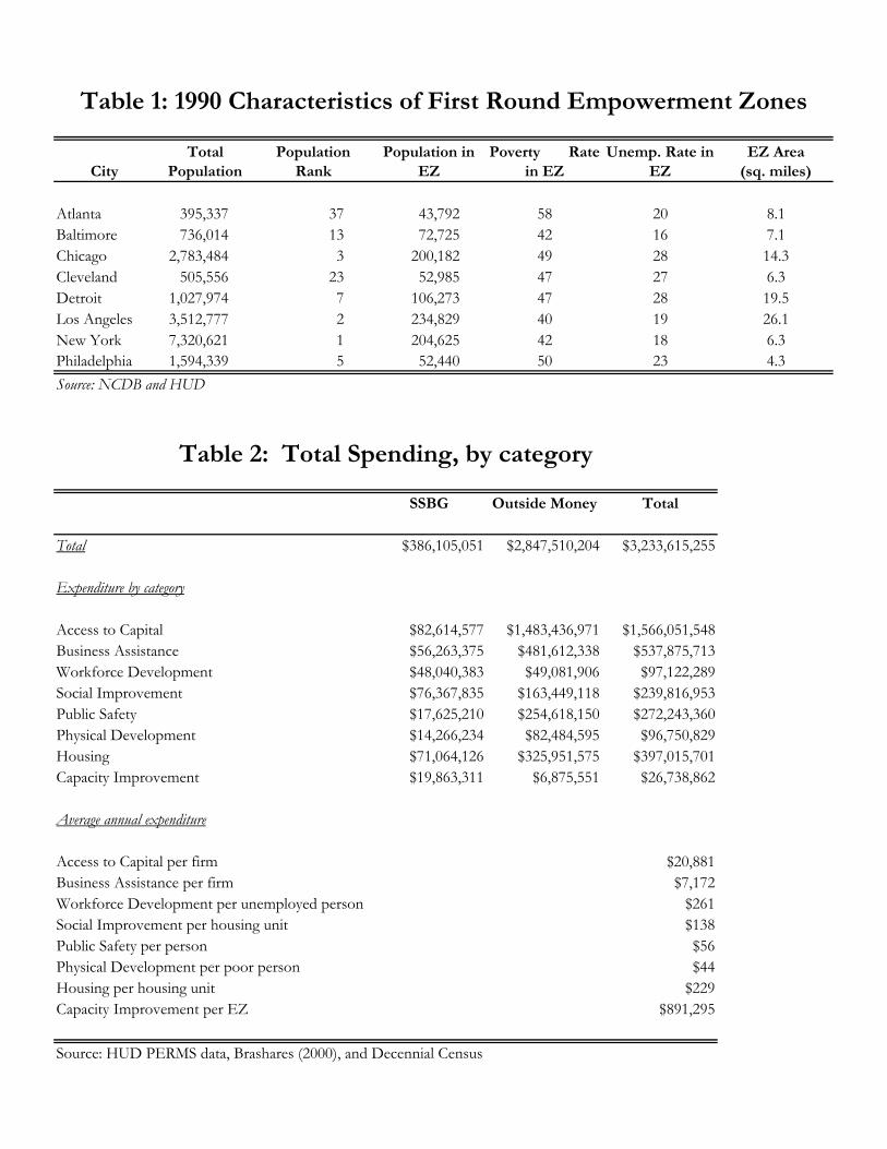
CityTotal

Population Population

RankPopulation in

EZ Poverty Rate

in EZUnemp. Rate in

EZEZ Area

(sq. miles)

Atlanta 395,337 37 43,792 58 20 8.1Baltimore 736,014 13 72,725 42 16 7.1Chicago 2,783,484 3 200,182 49 28 14.3Cleveland 505,556 23 52,985 47 27 6.3Detroit 1,027,974 7 106,273 47 28 19.5Los Angeles 3,512,777 2 234,829 40 19 26.1New York 7,320,621 1 204,625 42 18 6.3Philadelphia 1,594,339 5 52,440 50 23 4.3Source: NCDB and HUD

SSBG Outside Money Total

Total $386,105,051 $2,847,510,204 $3,233,615,255

Expenditure by category

Access to Capital $82,614,577 $1,483,436,971 $1,566,051,548Business Assistance $56,263,375 $481,612,338 $537,875,713Workforce Development $48,040,383 $49,081,906 $97,122,289Social Improvement $76,367,835 $163,449,118 $239,816,953Public Safety $17,625,210 $254,618,150 $272,243,360Physical Development $14,266,234 $82,484,595 $96,750,829Housing $71,064,126 $325,951,575 $397,015,701Capacity Improvement $19,863,311 $6,875,551 $26,738,862

Average annual expenditure

Access to Capital per firm $20,881Business Assistance per firm $7,172Workforce Development per unemployed person $261Social Improvement per housing unit $138Public Safety per person $56Physical Development per poor person $44Housing per housing unit $229Capacity Improvement per EZ $891,295

Source: HUD PERMS data, Brashares (2000), and Decennial Census

Table 1: 1990 Characteristics of First Round Empowerment Zones

Table 2: Total Spending, by category

EZ's Rejected/Future Zones

(outside EZ cities)

Rejected/Future Zones

(inside EZ cities)

Rejected/Future Zones

Rejected/Future Zones

Reweighted

Unproposed tracts in

treated cities

[1] [2] [3] [4] [5] [6]

Mean (census tracts)

% Black 0.686 0.540 0.717 0.570 0.677 0.298Employment Rate 0.379 0.466 0.438 0.461 0.380 0.559Log(pop) 7.747 7.931 8.068 7.954 7.863 7.954Log(Rent) 5.857 5.838 5.988 5.863 5.907 6.272Log(House Value) 10.701 10.829 10.654 10.800 10.593 11.760Log(Mean Earnings) 9.637 9.591 9.684 9.606 9.627 10.013Poverty Rate 0.460 0.395 0.388 0.393 0.446 0.188% Vacant Houses 0.147 0.141 0.121 0.138 0.135 0.069Unemployment Rate 0.231 0.160 0.206 0.167 0.232 0.100% In same house 0.560 0.494 0.570 0.506 0.555 0.579

% Travel less 20 min 0.473 0.668 0.447 0.632 0.466 0.429Prop. age 65+ 0.312 0.299 0.325 0.304 0.316 0.232Prop. female-headed HH 0.623 0.555 0.593 0.562 0.631 0.326Prop. Latino population 0.220 0.176 0.177 0.176 0.246 0.199Prop. age <18 0.118 0.121 0.103 0.118 0.103 0.127% College 0.056 0.090 0.060 0.085 0.053 0.196% High school dropouts 0.311 0.260 0.291 0.265 0.319 0.191Prop. of HHs with public assistance 0.353 0.241 0.293 0.250 0.362 0.135

Mean (city)

Avg. across tracts % black 0.438 0.307 0.480 0.335 0.447 0.333Total crime / population* 100 0.081 0.105 0.093 0.103 0.083 0.081% College degree 0.175 0.143 0.168 0.147 0.173 0.148% of workers in city government 0.049 0.047 0.043 0.046 0.047 0.079

Observations (number of census tracts) 257 1364 271 1635 1635 4495

Table 3: Sample Characteristics (1990)

Model Naïve Reweighted Blinder-Oaxaca B.O. City Pop.[1] [2] [3] [4]

Log(pop) Coeff. -0.022 -0.027 0.014 -0.057CI [ -0.071 , 0.018 ] [ -0.141 , 0.099 ] [ -0.083 , 0.113 ] [ -0.293 , 0.373 ]p-val 0.283 0.559 0.753 0.574

% In same house Coeff. 0.005 -0.005 -0.007 -0.021CI [ -0.013 , 0.030 ] [ -0.073 , 0.046 ] [ -0.046 , 0.038 ] [ -0.140 , 0.062 ]p-val 0.692 0.747 0.898 0.541

% Black Coeff. 0.002 -0.016 -0.003 -0.020CI [ -0.032 , 0.037 ] [ -0.065 , 0.017 ] [ -0.030 , 0.028 ] [ -0.113 , 0.112 ]p-val 0.797 0.270 0.990 0.583

% College Coeff. -0.010*** 0.008* 0.000 0.009CI [ -0.016 , -0.005 ] [ 0.004 , 0.043 ] [ -0.020 , 0.017 ] [ -0.092 , 0.067 ]p-val 0.000 0.014 0.998 0.758

Employment Rate Coeff. -0.010 0.017 0.017 0.038CI [ -0.043 , 0.030 ] [ -0.008 , 0.075 ] [ -0.007 , 0.052 ] [ -0.065 , 0.142 ]p-val 0.695 0.118 0.152 0.227

Unemployment Rate Coeff. -0.011 -0.002 -0.005 -0.004CI [ -0.034 , 0.019 ] [ -0.047 , 0.033 ] [ -0.038 , 0.020 ] [ -0.117 , 0.056 ]p-val 0.427 0.886 0.635 0.829

Log(Mean Earnings) Coeff. 0.003 0.111* 0.028 0.064CI [ -0.055 , 0.049 ] [ 0.072 , 0.297 ] [ -0.078 , 0.097 ] [ -0.204 , 0.243 ]p-val 0.972 0.006 0.624 0.464

Poverty Rate Coeff. 0.016 -0.010 -0.013 -0.064CI [ -0.014 , 0.042 ] [ -0.060 , 0.045 ] [ -0.056 , 0.026 ] [ -0.166 , 0.159 ]p-val 0.331 0.533 0.406 0.325

Log(House Value) Coeff. 0.118 0.095 -0.009 0.149CI [ -0.023 , 0.309 ] [ -0.027 , 0.470 ] [ -0.203 , 0.223 ] [ -0.727 , 0.522 ]p-val 0.092 0.092 0.958 0.561

Log(Rent) Coeff. -0.063* 0.029 0.030 0.121CI [ -0.110 , -0.009 ] [ -0.061 , 0.099 ] [ -0.021 , 0.101 ] [ -0.100 , 0.380 ]p-val 0.022 0.414 0.196 0.180

% Vacant Houses Coeff. 0.029* 0.015 -0.005 0.009CI [ 0.006 , 0.056 ] [ -0.019 , 0.043 ] [ -0.045 , 0.028 ] [ -0.098 , 0.090 ]p-val 0.014 0.288 0.662 0.817

Number of Tracts 1635 1502 1625 1625Number of Cities 79 79 79 79

Estimators: All columns show difference-in-difference estimates in which the change in outcomes over the period 1990-2000 amongcontrol tracts in cities winning an EZ is compared with the change in outcomes among control tracts in rejected and future zones in othercities. [1] Naïve refers to difference in difference estimates without covariate adjustments. [2] Reweighted refers to propensity scorereweighted estimates in which the propensity score was calculated using 1990 and 1980 tract and city level characteristics. [3] Blinder-Oaxaca computes counterfactual means of control tracts in treated cities via regression methods. [4] B.O. City Pop. is the Blinder-Oaxaca estimatoraugmented to include a 3rd order polynomial in 1990 city population. (See Sections IV-B, V-A and Appendix V for details).Inference: 95% Confidence intervals (CI) and p-values were obtained via a pairwise block bootstrap that resampled zones in order to preservethe within zone dependence of the data. See Appendix IV for details. Significance levels . A multiple testing procedure described in theAppendix was used to control the False Discovery Rate (FDR) to prespecified levels. The procedure yields lower threshold p-values forfixed level tests than in the single equation case. Stars indicate that a hypothesis can be rejected while controlling the FDR to specifiedlevels: * rejected at 10% FDR, ** rejected at 5% FDR and *** rejected at 1% FDR.

Difference-in-Differences EstimatesTable 4: Balance of Control Samples

Model Naïve Reweighted Blinder-Oaxaca B.O. City Pop.[1] [2] [3] [4]

Log(pop) Coeff. -0.035 0.005 0.024 0.049CI [ -0.109 , 0.056 ] [ -0.085 , 0.105 ] [ -0.040 , 0.096 ] [ -0.024 , 0.187 ]p-val 0.427 0.839 0.472 0.167

% In same house Coeff. -0.009 -0.014 0.001 0.003CI [ -0.036 , 0.013 ] [ -0.052 , 0.006 ] [ -0.022 , 0.021 ] [ -0.023 , 0.032 ]p-val 0.476 0.092 0.972 0.879

% Black Coeff. -0.037 -0.026** -0.012 -0.020CI [ -0.074 , 0.011 ] [ -0.069 , -0.005 ] [ -0.036 , 0.014 ] [ -0.048 , 0.011 ]p-val 0.131 0.026 0.346 0.164

% College Coeff. 0.010 0.023** 0.012 0.014CI [ -0.005 , 0.025 ] [ 0.010 , 0.047 ] [ -0.004 , 0.024 ] [ -0.006 , 0.027 ]p-val 0.180 0.011 0.157 0.163

Employment Rate Coeff. 0.040** 0.038*** 0.020* 0.023CI [ 0.010 , 0.074 ] [ 0.025 , 0.084 ] [ 0.003 , 0.041 ] [ 0.002 , 0.050 ]p-val 0.009 0.000 0.022 0.039

Unemployment Rate Coeff. -0.041** -0.040** -0.031** -0.034*CI [ -0.072 , -0.013 ] [ -0.079 , -0.019 ] [ -0.053 , -0.013 ] [ -0.057 , -0.012 ]p-val 0.005 0.012 0.003 0.007

Log(Mean Earnings) Coeff. 0.012 0.017 0.028 0.029CI [ -0.068 , 0.100 ] [ -0.050 , 0.114 ] [ -0.044 , 0.093 ] [ -0.049 , 0.102 ]p-val 0.759 0.543 0.425 0.348

Poverty Rate Coeff. -0.049*** -0.050*** -0.038** -0.044CI [ -0.091 , -0.016 ] [ -0.103 , -0.028 ] [ -0.058 , -0.013 ] [ -0.067 , -0.007 ]p-val 0.000 0.000 0.008 0.030

Log(House Value) Coeff. 0.297*** 0.224** 0.158 0.183CI [ 0.093 , 0.538 ] [ 0.078 , 0.506 ] [ 0.006 , 0.332 ] [ 0.005 , 0.367 ]p-val 0.001 0.020 0.040 0.044

Log(Rent) Coeff. 0.005 0.077*** 0.044 0.054CI [ -0.061 , 0.070 ] [ 0.053 , 0.155 ] [ -0.001 , 0.099 ] [ -0.003 , 0.130 ]p-val 0.896 0.001 0.056 0.061

% Vacant Houses Coeff. 0.023 -0.001 0.014 0.006CI [ -0.006 , 0.048 ] [ -0.036 , 0.025 ] [ -0.007 , 0.037 ] [ -0.031 , 0.027 ]p-val 0.128 0.681 0.177 0.790

Number of Tracts 1892 1869 1892 1892Number of Cities 82 82 82 82

Inference: 95% Confidence intervals (CI) and p-values were obtained via a pairwise block bootstrap that resampled zones in order to preserve thewithin zone dependence of the data. See Appendix IV for details. Significance levels . A multiple testing procedure described in the Appendix wasused to control the False Discovery Rate (FDR) to prespecified levels. The procedure yields lower threshold p-values for fixed level tests than inthe single equation case. Stars indicate that a hypothesis can be rejected while controlling the FDR to specified levels: * rejected at 10% FDR, **rejected at 5% FDR and *** rejected at 1% FDR.

Table 5: Impact of EZ DesignationDifference-in-Differences Estimates

Estimators: All columns show difference-in-difference estimates in which the change in outcomes over the period 1990-2000 among EZ tractsis compared with the change in outcomes among tracts in rejected and future zones. [1] Naïve refers to difference in difference estimateswithout covariate adjustment. [2] Reweighted refers to propensity score reweighted estimates in which the propensity score was calculated using1990 and 1980 tract and city level characteristics. [3] Blinder-Oaxaca computes counterfactual means of EZ tracts via regression methods. [4] B.O. City Pop. is the Blinder-Oaxaca estimator augmented to include a 3rd order polynomial in 1990 city population. (See Section IV-B andAppendix V for details).

Model Naïve Reweighted Blinder-Oaxaca B.O. City Pop.[1] [2] [3] [4]

Log(pop) Coeff. -0.055 0.018 0.016 0.020CI [ -0.235 , 0.079 ] [ -0.081 , 0.122 ] [ -0.069 , 0.126 ] [ -0.069 , 0.114 ]p-val 0.589 0.621 0.597 0.533

% In same house Coeff. 0.010 0.001 0.012 0.012CI [ -0.012 , 0.041 ] [ -0.033 , 0.029 ] [ -0.027 , 0.045 ] [ -0.030 , 0.046 ]p-val 0.404 0.794 0.567 0.609

% Black Coeff. -0.050 -0.024 -0.018 -0.017CI [ -0.109 , 0.036 ] [ -0.068 , 0.011 ] [ -0.066 , 0.022 ] [ -0.061 , 0.010 ]p-val 0.228 0.170 0.385 0.185

% College Coeff. 0.003 0.001 0.004 0.009CI [ -0.007 , 0.011 ] [ -0.012 , 0.009 ] [ -0.010 , 0.013 ] [ -0.009 , 0.018 ]p-val 0.460 0.681 0.643 0.258

Employment Rate Coeff. 0.015 -0.016 -0.017 -0.012CI [ -0.015 , 0.039 ] [ -0.058 , -0.001 ] [ -0.042 , 0.015 ] [ -0.041 , 0.021 ]p-val 0.338 0.046 0.248 0.410

Unemployment Rate Coeff. 0.010 0.012 0.004 -0.006CI [ -0.009 , 0.035 ] [ 0.001 , 0.054 ] [ -0.020 , 0.035 ] [ -0.031 , 0.026 ]p-val 0.314 0.045 0.633 0.758

Log(Mean Earnings) Coeff. 0.007 -0.013 0.019 0.037CI [ -0.076 , 0.064 ] [ -0.109 , 0.049 ] [ -0.068 , 0.085 ] [ -0.060 , 0.115 ]p-val 0.836 0.578 0.687 0.364

Poverty Rate Coeff. -0.022 0.034* 0.020 0.010CI [ -0.050 , 0.011 ] [ 0.021 , 0.087 ] [ -0.019 , 0.059 ] [ -0.028 , 0.050 ]p-val 0.206 0.005 0.238 0.448

Log(House Value) Coeff. 0.091 -0.050 -0.087 -0.100CI [ -0.124 , 0.284 ] [ -0.282 , 0.134 ] [ -0.292 , 0.170 ] [ -0.300 , 0.148 ]p-val 0.400 0.515 0.442 0.391

Log(Rent) Coeff. 0.036 -0.041 -0.006 -0.011CI [ -0.078 , 0.129 ] [ -0.139 , 0.005 ] [ -0.085 , 0.102 ] [ -0.084 , 0.092 ]p-val 0.502 0.063 0.931 0.817

% Vacant Houses Coeff. -0.002 0.015 -0.002 -0.004CI [ -0.029 , 0.027 ] [ -0.011 , 0.041 ] [ -0.032 , 0.017 ] [ -0.031 , 0.018 ]p-val 0.992 0.247 0.710 0.593

Number of Tracts 1891 1882 1891 1891Number of Cities 82 82 82 82

Table 6: False Experiment I (Lagged Model)Difference-in-Differences Estimates

Inference: 95% Confidence intervals (CI) and p-values were obtained via a pairwise block bootstrap that resampled zones in order topreserve the within zone dependence of the data. See Appendix IV for details. Significance levels . A multiple testing proceduredescribed in the Appendix was used to control the False Discovery Rate (FDR) to prespecified levels. The procedure yields lowerthreshold p-values for fixed level tests than in the single equation case. Stars indicate that a hypothesis can be rejected whilecontrolling the FDR to specified levels: * rejected at 10% FDR, ** rejected at 5% FDR and *** rejected at 1% FDR.

Estimators: All columns show difference-in-difference estimates in which the change in outcomes over the period 1980-1990among EZ tracts is compared with the change in outcomes among tracts in rejected and future zones. [1] Naïve refers todifference in difference estimates without covariate adjustment. [2] Reweighted refers to propensity score reweighted estimates inwhich the propensity score was calculated using 1980 and 1970 tract and city level characteristics. [3] Blinder-Oaxaca computescounterfactual means of EZ tracts via regression methods. [4] B.O. City Pop. is the Blinder-Oaxaca estimator augmented toinclude a 3rd order polynomial in 1980 city population. (See Sections IV-B, V-C and Appendix V for details).

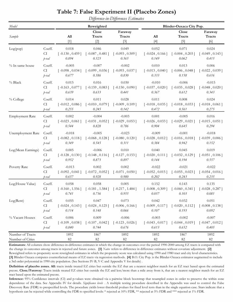
Model

Sample AllClose Tracts

Faraway Tracts All

Close Tracts

Faraway Tracts

[1] [2] [3] [4] [5] [6]

Log(pop) Coeff. 0.018 0.046 0.049 0.052 0.071 0.024CI [ -0.130 , 0.459 ] [ -0.087 , 0.481 ] [ -0.093 , 0.509 ] [ -0.024 , 0.166 ] [ -0.004 , 0.203 ] [ -0.049 , 0.143 ]p-val 0.894 0.523 0.565 0.149 0.062 0.415

% In same house Coeff. -0.005 -0.007 -0.002 0.010 0.013 0.006CI [ -0.098 , 0.034 ] [ -0.099 , 0.036 ] [ -0.093 , 0.037 ] [ -0.013 , 0.040 ] [ -0.006 , 0.048 ] [ -0.022 , 0.039 ]p-val 0.677 0.586 0.830 0.333 0.158 0.616

% Black Coeff. 0.015 0.016 0.030 -0.010 -0.006 -0.015CI [ -0.163 , 0.077 ] [ -0.159 , 0.083 ] [ -0.150 , 0.090 ] [ -0.037 , 0.020 ] [ -0.035 , 0.028 ] [ -0.048 , 0.020 ]p-val 0.639 0.633 0.441 0.367 0.612 0.343

% College Coeff. 0.014 0.011 0.028 0.011 0.008 0.024CI [ -0.012 , 0.086 ] [ -0.010 , 0.079 ] [ -0.009 , 0.109 ] [ -0.018 , 0.035 ] [ -0.018 , 0.033 ] [ -0.018 , 0.061 ]p-val 0.255 0.245 0.142 0.472 0.561 0.275

Employment Rate Coeff. 0.002 -0.004 -0.003 0.001 -0.005 0.016CI [ -0.023 , 0.061 ] [ -0.031 , 0.052 ] [ -0.029 , 0.053 ] [ -0.026 , 0.033 ] [ -0.029 , 0.021 ] [ -0.015 , 0.051 ]p-val 0.544 0.828 0.786 0.904 0.645 0.294

Unemployment Rate Coeff. -0.018 -0.005 -0.023 -0.009 -0.001 -0.018CI [ -0.082 , 0.118 ] [ -0.068 , 0.128 ] [ -0.080 , 0.120 ] [ -0.028 , 0.012 ] [ -0.016 , 0.018 ] [ -0.039 , 0.006 ]p-val 0.349 0.545 0.311 0.384 0.942 0.152

Log(Mean Earnings) Coeff. 0.005 -0.006 0.010 0.040 0.045 0.019CI [ -0.128 , 0.130 ] [ -0.148 , 0.116 ] [ -0.127 , 0.153 ] [ -0.020 , 0.111 ] [ -0.032 , 0.129 ] [ -0.051 , 0.106 ]p-val 0.952 0.873 0.897 0.144 0.194 0.557

Poverty Rate Coeff. -0.013 0.002 0.002 -0.022 -0.021 -0.022CI [ -0.092 , 0.041 ] [ -0.072 , 0.052 ] [ -0.071 , 0.050 ] [ -0.052 , 0.015 ] [ -0.055 , 0.023 ] [ -0.054 , 0.016 ]p-val 0.657 0.928 0.980 0.202 0.243 0.235

Log(House Value) Coeff. 0.058 0.058 0.005 0.152 0.143 0.135CI [ -0.160 , 1.556 ] [ -0.181 , 1.584 ] [ -0.217 , 1.484 ] [ -0.008 , 0.309 ] [ -0.060 , 0.341 ] [ -0.028 , 0.287 ]p-val 0.741 0.736 0.955 0.057 0.103 0.081

Log(Rent) Coeff. 0.055 0.047 0.073 0.042 0.032 0.051CI [ -0.024 , 0.143 ] [ -0.024 , 0.125 ] [ -0.006 , 0.166 ] [ -0.009 , 0.117 ] [ -0.020 , 0.112 ] [ -0.008 , 0.138 ]p-val 0.114 0.148 0.066 0.107 0.193 0.092

% Vacant Houses Coeff. 0.006 0.009 -0.006 -0.003 -0.002 -0.007CI [ -0.109 , 0.038 ] [ -0.107 , 0.042 ] [ -0.123 , 0.026 ] [ -0.043 , 0.017 ] [ -0.044 , 0.019 ] [ -0.047 , 0.012 ]p-val 0.840 0.744 0.676 0.613 0.652 0.405

Number of Tracts 1892 1867 1892 1892 1867 1892Number of Cities 82 82 82 82 82 82

Inference: 95% Confidence intervals (CI) and p-values were obtained via a pairwise block bootstrap that resampled zones in order to preserve the within zonedependence of the data. See Appendix IV for details. Significance levels . A multiple testing procedure described in the Appendix was used to control the FalseDiscovery Rate (FDR) to prespecified levels. The procedure yields lower threshold pvalues for fixed level tests than in the single equation case. Stars indicate that ahypothesis can be rejected while controlling the FDR to specified levels: * rejected at 10% FDR, ** rejected at 5% FDR and *** rejected at 1% FDR.

Estimators: All columns show difference-in-difference estimates in which the change in outcomes over the period 1990-2000 among EZ tracts is compared with the change in outcomes among tracts in rejected and future zones. [1] Naïve refers to difference in difference estimates without covariate adjustment. [2] Reweighted refers to propensity score reweighted estimates in which the propensity score was calculated using 1990 and 1980 tract and city level characteristics. [3] Blinder-Oaxaca computes counterfactual means of EZ tracts via regression methods. [4] B.O. City Pop. is the Blinder-Oaxaca estimator augmented to include a 3rd order polynomial in 1990 city population. (See Sections IV-B, V-C and Appendix V for details) .

Table 7: False Experiment II (Placebo Zones)Difference-in-Differences Estimates

Blinder-Oaxaca City Pop.

Definition of placebo zones. All: tracts inside treated EZ cities but outside the EZ that are a nearest neighbor match for an EZ tract based upon the estimatedpscore. Close/Faraway: Tracts inside treated EZ cities but outside the EZ and less/more than a mile away from it, that are a nearest neighbor match for an EZtract based upon the estimated pscore.

Reweighted

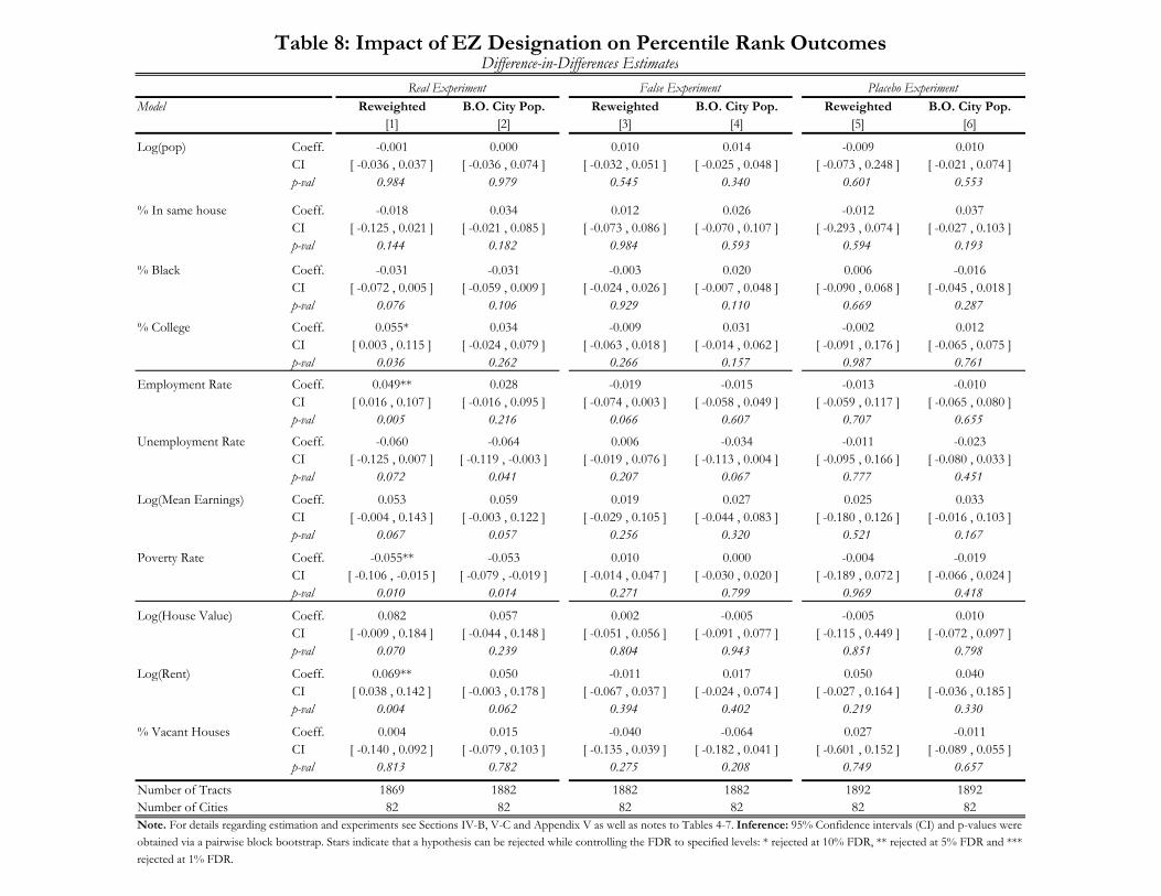
Model Reweighted B.O. City Pop. Reweighted B.O. City Pop. Reweighted B.O. City Pop.[1] [2] [3] [4] [5] [6]

Log(pop) Coeff. -0.001 0.000 0.010 0.014 -0.009 0.010CI [ -0.036 , 0.037 ] [ -0.036 , 0.074 ] [ -0.032 , 0.051 ] [ -0.025 , 0.048 ] [ -0.073 , 0.248 ] [ -0.021 , 0.074 ]p-val 0.984 0.979 0.545 0.340 0.601 0.553

% In same house Coeff. -0.018 0.034 0.012 0.026 -0.012 0.037CI [ -0.125 , 0.021 ] [ -0.021 , 0.085 ] [ -0.073 , 0.086 ] [ -0.070 , 0.107 ] [ -0.293 , 0.074 ] [ -0.027 , 0.103 ]p-val 0.144 0.182 0.984 0.593 0.594 0.193

% Black Coeff. -0.031 -0.031 -0.003 0.020 0.006 -0.016CI [ -0.072 , 0.005 ] [ -0.059 , 0.009 ] [ -0.024 , 0.026 ] [ -0.007 , 0.048 ] [ -0.090 , 0.068 ] [ -0.045 , 0.018 ]p-val 0.076 0.106 0.929 0.110 0.669 0.287

% College Coeff. 0.055* 0.034 -0.009 0.031 -0.002 0.012CI [ 0.003 , 0.115 ] [ -0.024 , 0.079 ] [ -0.063 , 0.018 ] [ -0.014 , 0.062 ] [ -0.091 , 0.176 ] [ -0.065 , 0.075 ]p-val 0.036 0.262 0.266 0.157 0.987 0.761

Employment Rate Coeff. 0.049** 0.028 -0.019 -0.015 -0.013 -0.010CI [ 0.016 , 0.107 ] [ -0.016 , 0.095 ] [ -0.074 , 0.003 ] [ -0.058 , 0.049 ] [ -0.059 , 0.117 ] [ -0.065 , 0.080 ]p-val 0.005 0.216 0.066 0.607 0.707 0.655

Unemployment Rate Coeff. -0.060 -0.064 0.006 -0.034 -0.011 -0.023CI [ -0.125 , 0.007 ] [ -0.119 , -0.003 ] [ -0.019 , 0.076 ] [ -0.113 , 0.004 ] [ -0.095 , 0.166 ] [ -0.080 , 0.033 ]p-val 0.072 0.041 0.207 0.067 0.777 0.451

Log(Mean Earnings) Coeff. 0.053 0.059 0.019 0.027 0.025 0.033CI [ -0.004 , 0.143 ] [ -0.003 , 0.122 ] [ -0.029 , 0.105 ] [ -0.044 , 0.083 ] [ -0.180 , 0.126 ] [ -0.016 , 0.103 ]p-val 0.067 0.057 0.256 0.320 0.521 0.167

Poverty Rate Coeff. -0.055** -0.053 0.010 0.000 -0.004 -0.019CI [ -0.106 , -0.015 ] [ -0.079 , -0.019 ] [ -0.014 , 0.047 ] [ -0.030 , 0.020 ] [ -0.189 , 0.072 ] [ -0.066 , 0.024 ]p-val 0.010 0.014 0.271 0.799 0.969 0.418

Log(House Value) Coeff. 0.082 0.057 0.002 -0.005 -0.005 0.010CI [ -0.009 , 0.184 ] [ -0.044 , 0.148 ] [ -0.051 , 0.056 ] [ -0.091 , 0.077 ] [ -0.115 , 0.449 ] [ -0.072 , 0.097 ]p-val 0.070 0.239 0.804 0.943 0.851 0.798

Log(Rent) Coeff. 0.069** 0.050 -0.011 0.017 0.050 0.040CI [ 0.038 , 0.142 ] [ -0.003 , 0.178 ] [ -0.067 , 0.037 ] [ -0.024 , 0.074 ] [ -0.027 , 0.164 ] [ -0.036 , 0.185 ]p-val 0.004 0.062 0.394 0.402 0.219 0.330

% Vacant Houses Coeff. 0.004 0.015 -0.040 -0.064 0.027 -0.011CI [ -0.140 , 0.092 ] [ -0.079 , 0.103 ] [ -0.135 , 0.039 ] [ -0.182 , 0.041 ] [ -0.601 , 0.152 ] [ -0.089 , 0.055 ]p-val 0.813 0.782 0.275 0.208 0.749 0.657

Number of Tracts 1869 1882 1882 1882 1892 1892Number of Cities 82 82 82 82 82 82

Table 8: Impact of EZ Designation on Percentile Rank OutcomesDifference-in-Differences Estimates

Note. For details regarding estimation and experiments see Sections IV-B, V-C and Appendix V as well as notes to Tables 4-7. Inference: 95% Confidence intervals (CI) and p-values were obtained via a pairwise block bootstrap. Stars indicate that a hypothesis can be rejected while controlling the FDR to specified levels: * rejected at 10% FDR, ** rejected at 5% FDR and *** rejected at 1% FDR.

Placebo ExperimentFalse ExperimentReal Experiment

Model Reweighted B.O. City Pop. Reweighted B.O. City Pop.[1] [2] [3] [4]

Employment Rate Coeff. 0.033*** 0.024 -0.002 0.004CI [ 0.019 , 0.079 ] [ 0.000 , 0.054 ] [ -0.031 , 0.061 ] [ -0.025 , 0.040 ]p-val 0.001 0.053 0.867 0.760

Unemployment Rate Coeff. -0.029** -0.023 -0.014 -0.003CI [ -0.066 , -0.003 ] [ -0.044 , 0.000 ] [ -0.078 , 0.141 ] [ -0.020 , 0.016 ]p-val 0.035 0.047 0.442 0.797

Poverty Rate Coeff. -0.045*** -0.036 -0.012 -0.022CI [ -0.097 , -0.025 ] [ -0.061 , 0.001 ] [ -0.109 , 0.043 ] [ -0.057 , 0.016 ]p-val 0.000 0.055 0.653 0.198

Employment Rate 16-19 in HS Coeff. -0.003 -0.008 0.022 0.009CI [ -0.059 , 0.061 ] [ -0.105 , 0.029 ] [ -0.042 , 0.164 ] [ -0.069 , 0.055 ]p-val 0.804 0.507 0.277 0.855

Employment Rate 16-19 HS drop. Coeff. 0.103** 0.101 0.040 0.062CI [ 0.039 , 0.193 ] [ -0.072 , 0.188 ] [ -0.117 , 0.165 ] [ -0.104 , 0.163 ]p-val 0.008 0.143 0.570 0.337

Employment Rate 16-19 HS grad. Coeff. 0.129** 0.096 0.032 0.062CI [ 0.046 , 0.369 ] [ -0.040 , 0.300 ] [ -0.132 , 0.360 ] [ -0.064 , 0.199 ]p-val 0.012 0.141 0.529 0.318

% College Coeff. 0.012 -0.018 0.010 0.029CI [ -0.022 , 0.040 ] [ -0.083 , 0.084 ] [ -0.030 , 0.054 ] [ -0.042 , 0.092 ]p-val 0.443 0.472 0.621 0.306

Number of Tracts 1869 1869 1892 1892Number of Cities 82 82 82 82

Note: Racial-composition-constant outcomes fix the racial composition of a census tract to that observed in 1990. For details see Sections IV-B, V-D and Appendix V as well as notes to Tables 4-7. Inference: 95% Confidence intervals (CI) and p-values were obtained via a pairwise block bootstrap. Stars indicate that a hypothesis can be rejected while controlling the FDR to specified levels: * rejected at 10% FDR, ** rejected at 5% FDR and *** rejected at 1% FDR.

Real Experiment Placebo Experiment

Table 9: Composition-Constant Impact of EZ DesignationDifference-in-Differences Estimates

Panel (A) Decennial census data (inside Empowerment Zones, 1990) Notes

Population Total Population 967,851Total Population 16+ 718,202

Employed 259,271Persons in labor force 330,373

Earnings Average annual wage (in 1990 dollars) 16,182

Panel (B) Estimated effects of the Empowerment Zones program

Labor Market Decrease in the unemployed between 1995 and 2000 13,215 0.041 x Persons in labor force

Decrease in poverty headcount between 1995 and 2000 48,393 0.049 x Total population

Employment Increase between 1995 and 2000 27,292 0.039 x Population 16+

Wage value of the number of jobs created 441,634,034 (0.039 x Population 16+) x Ave. Annual wage

Present discounted value of jobs created 1,104,085,085 Wage value/[1-β(1-d)], with d=1/3 (separation rate) and β=0.9 (social disc. factor)

Housing Market Average change in annual tractwide rent 319 0.077 * Median annual rent inside EZs

Total increase in annual rents inside EZ 78,011,523 Average increase in monthly rent x 12 x # of rented houses

Present Value 780,115,228 Total Annual Rents / 0.1

Average change in tract-wide owner occupied housing value 9,707 0.224 * Median housing value inside EZs

Total increase in owner-occupied housing value inside EZ 474,497,043 Average change in tract-wide value x # of owner occupied houses

Total increase of value of EZ housing units 1,254,612,272 Increase in rent asset value + Increase in value benefiting EZ residents

Note: The coefficients 0.040 (for unemployment rate), 0.050 (for poverty rate), and 0.038 (for employment rate), 0.077 (for rent) and 0.224 (for housing values) were obtained from Column 2 of Table 5.

Table 10: Impact Calculations

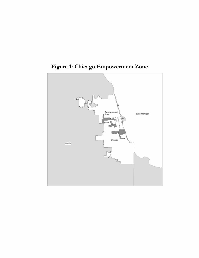
Figure 1: Chicago Empowerment Zone

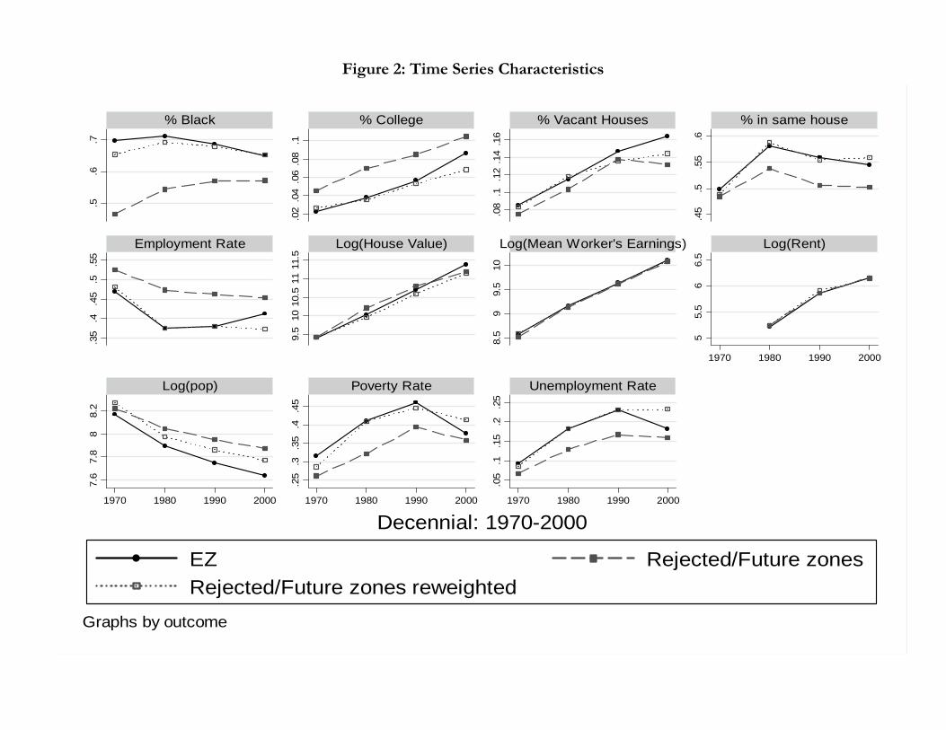
Figure 2: Time Series Characteristics.5

.6.7

.02

.04

.06

.08

.1

.08

.1.1

2.1

4.1

6

.45

.5.5

5.6

.35

.4.4

5.5

.55

9.5

1010

.511

11.5

8.5

99.

510

55.

56

6.5

7.6

7.8

88.

2

.25

.3.3

5.4

.45

.05

.1.1

5.2

.25

1970 1980 1990 2000

1970 1980 1990 2000 1970 1980 1990 2000 1970 1980 1990 2000

% Black % College % Vacant Houses % in same house

Employment Rate Log(House Value) Log(Mean Worker's Earnings) Log(Rent)

Log(pop) Poverty Rate Unemployment Rate

EZ Rejected/Future zonesRejected/Future zones reweighted

Decennial: 1970-2000

Graphs by outcome

Chicago - Empowerment Zoneand Placebo Tracts

Placebo Tracts

Empowerment Zone

Figure 3Chicago: Empowerment Zone and Placebo Tracts

Empowerment Zone

Placebo Tracts

CityEZ (Round

I) (1994)Application

(1994)Round 1

(1994)Round 2

(2000)Round 3

(2002) City

EZ (Round I)

(1994)Application

(1994)Round 1

(1994)Round 2

(2000)Round 3

(2002)

Akron x EC-1 Memphis x RCAlbany x EC-1 Miami x EC-1 EZ-2Albuquerque x EC-1 Milwaukee x RCAnniston x Minneapolis x EC-1 EZ-2Atlanta x x Mobile x RCAustin x Monroe x RCBaltimore x x Muskegon x EC-1Benton Harbor x Nashville-Davidso x EC-1Birmingham x EC-1 New Haven x EC-1 EZ-2Boston x EEC-1 EZ-2 New Orleans x RCBridgeport x EC-1 New York x xBuffalo RC Newburgh x EC-1Charleston x RC Niagara Falls RCCharlotte x EC-1 Norfolk x EC-1 EZ-2Chattanooga RC Oakland x EEC-1Chester x Ogden x EC-1Chicago x x RC Oklahoma x EC-1 EZ-3Cincinnati EZ-2 Omaha x EC-1Cleveland x x Orange xColumbia EZ-2 Peoria xColumbus EZ-2 Philadelphia x x RCCorpus Christi RC Phoenix x EC-1Cumberland EZ-2 Pine Bluff xDallas x EC-1 Pittsburgh x EC-1Denver x EC-1 Port Arthur xDes Moines x EC-1 Portland x EC-1Detroit x x RC Providence x EC-1El Paso x EC-1 EZ-2 Richmond xFairbanks x Rochester x RCFlint x RC Sacramento xFort Lauderdale x San Antonio x EC-1 EZ-3Fort Worth x San Diego x RCFresno x EZ-3 San Francisco RCGary x EZ-2 Santa Ana EZ-2Greeley x Savannah xHamilton RC Schenectady RCHarrisburg x EC-1 Seattle x EC-1Hartford x Shreveport xHouston x EEC-1 Sioux xHuntington EZ-2 Springfield x EC-1Indianapolis x EC-1 St. Louis x EC-1 EZ-2Jackson x EC-1 St. Paul x EC-1Jacksonville x EZ-3 Steubenville xKansas x EEC-1 Syracuse EZ-3Knoxville x EZ-2 Tacoma x RCLake Charles x Tampa x EC-1Las Vegas x EC-1 Tucson x EZ-3Lawrence RC Waco x EC-1Little Rock x EC-1 EZ-3 Washington x EC-1 UEnZLos Angeles x x RC Wilmington x EC-1Louisville x EC-1 Yakima RCLowell RC Yonkers EZ-3Manchester x EC-1 Youngstown

Note: EC-1 refers to Enterprise Community awarded in Round I (1994), EEC-1 refers to Enhanced Enterprise Community awarded in Round I (1994), EZ-2refers to Empowrment Zone awarded in Round II (2000), RC refers to Renewal Community awarded in Round III (2002), EZ-3 refers to Empowrment Zoneawarded in Round III (2002) and UEnZ Urban Enterprise Zone awarded in Round III (2002)

Table A1: Treatment by city

Model: 1 Lag 2 Lags 1 Lag 2 LagsLinear models(1) Basic 1413 1347 1391 1308(2) Basic + Other outcomes 1405 1342 1366 1270(3) Basic + Other outcomes + Other tract-level covariates 1207 1236 1096 1025(4) Basic + Other outcomes + Other tract-level covariates + City covariates 1182 1135 1049 880

Linear + Squares models*(5) Basic 1413 1347 1391 1308(6) Basic + Other outcomes 1405 1342 1366 1270(7) Basic + Other outcomes + Other tract-level covariates 1207 1236 1096 1025

Covariates included in each model:

Table A2: Logit Model Selection

Note: * These models include linear and squared terms of tract level variables.

BIC AIC

Basic: Poverty Rate, Log(pop), Unemployment Rate.

Other outcomes: % Black, % Travel less 20 min, Employment Rate, Log(Rent), Log(House Value), Log(Mean Earnings), % Vacant Houses, % in same house, % College degree.

Other tract-level covariates: Prop. female-headed HH, Log family income*, Prop. Latino population, Prop. age <18, Prop. age 65+, % High school dropouts, Log rent, Log house value, Prop. of HHs with public assistance.

City level covariates: % black, Total crime / population* 100, % 65+ years old, % College degree, % of workers in manufacturing, % of workers in city government.

Baseline Big City All No NY-LA No CLE-LA Balance Baseline Big City All No NY-LA No CLE-LA% Black [1980] 1.482 1.889 0.275 -0.846 -2.834 -7.95 [1970] 1.184 1.179 0.692 1.311 2.044

[0.141] [0.056]* [0.717] [0.244] [0.454] [0.009]*** [0.086]* [0.090]* [0.400] [0.065]* [0.019]**[1990] -1.576 -1.856 -1.321 -0.647 1.404 3.832 [1980] -0.746 -0.716 -1.063 -1.984 -1.345

[0.210] [0.116] [0.231] [0.529] [0.711] [0.184] [0.413] [0.438] [0.216] [0.019]** [0.337]% College [1980] -7.112 -7.886 -5.638 -1.957 2.519 23.706 [1970] -10.398 -10.976 -12.682 -17.509 -15.034

[0.060]* [0.025]** [0.072]* [0.614] [0.599] [0.000]*** [0.006]*** [0.005]*** [0.024]** [0.001]*** [0.041]**[1990] 6.778 7.74 4.09 0.826 11.394 2.523 [1980] -0.422 -1.103 0.581 1.487 6.916

[0.078]* [0.035]** [0.139] [0.631] [0.006]*** [0.551] [0.871] [0.654] [0.840] [0.595] [0.074]*% High school dropouts [1980] -1.802 -2.17 1.477 1.25 7.615 9.024 [1970] 2.479 2.009 1.961 -1.265 0.56

[0.472] [0.419] [0.633] [0.701] [0.002]*** [0.020]** [0.612] [0.680] [0.723] [0.831] [0.866][1990] 5.056 5.105 6.461 6.242 6.84 -3.261 [1980] -0.119 -0.27 1.847 0.966 7.168

[0.035]** [0.022]** [0.021]** [0.056]* [0.006]*** [0.302] [0.975] [0.945] [0.623] [0.801] [0.015]**% Travel less 20 min [1980] 0.206 -0.154 -0.054 0.846 -2.376 -8.078 [1980] -2.238 -2.339 -1.542 -1.62 -5.95

[0.774] [0.823] [0.959] [0.376] [0.025]** [0.000]*** [0.024]** [0.009]*** [0.131] [0.201] [0.000]***[1990] -3.171 -3.725 -1.575 -3.411 -9.303 -19.747

[0.064]* [0.023]** [0.398] [0.053]* [0.000]*** [0.000]***% Vacant Houses [1980] -2.783 -3.286 -1.791 -2.364 -2.722 6.71 [1970] 0.307 0.024 3.722 0.459 1.174

[0.260] [0.169] [0.554] [0.408] [0.138] [0.001]*** [0.861] [0.990] [0.093]* [0.856] [0.608][1990] 2.577 2.314 4.714 4.456 0.986 -6.374 [1980] -3.98 -4.365 -3.865 -1.663 -6.137

[0.098]* [0.157] [0.000]*** [0.000]*** [0.671] [0.004]*** [0.044]** [0.045]** [0.093]* [0.466] [0.023]**% in same house [1980] -0.883 -0.987 -1.629 -2.122 4.448 4.872 [1970] 0.235 -0.285 0.094 -0.387 -0.119

[0.430] [0.335] [0.134] [0.027]** [0.000]*** [0.003]*** [0.863] [0.823] [0.957] [0.857] [0.936][1990] 2.667 2.246 3.029 2.211 4.59 7.93 [1980] -0.263 -0.418 -0.241 -0.587 2.679

[0.069]* [0.148] [0.031]** [0.137] [0.003]*** [0.007]*** [0.804] [0.718] [0.855] [0.705] [0.008]***Employment Rate [1980] -3.512 -4.222 -0.832 -4.855 -8.2 2.199 [1970] -1.044 -0.354 2.38 2.274 3.015

[0.225] [0.136] [0.814] [0.181] [0.040]** [0.438] [0.695] [0.897] [0.467] [0.541] [0.427][1990] 2.429 2.624 9.254 9.919 7.347 8.501 [1980] -2.772 -3.105 2.236 0.789 -5.462

[0.502] [0.490] [0.000]*** [0.000]*** [0.042]** [0.004]*** [0.513] [0.464] [0.460] [0.798] [0.225]Log(Area) [1980] -0.247 -0.181 -0.754 -0.678 -0.352 -0.615 [1970] -0.393 -0.36 -0.825 -0.99 -0.485

[0.469] [0.588] [0.002]*** [0.002]*** [0.187] [0.069]* [0.192] [0.238] [0.000]*** [0.000]*** [0.104]Log(House Value) [1980] -1.094 -1.036 -1.94 -2.047 -1.386 -1.732 [1980] -0.677 -0.711 -1.249 -0.732 -1.281

[0.005]*** [0.020]** [0.000]*** [0.000]*** [0.058]* [0.035]** [0.123] [0.118] [0.044]** [0.148] [0.069]*[1990] -0.396 -0.309 -0.866 -0.131 -2.022 -2.815

[0.387] [0.459] [0.111] [0.713] [0.000]*** [0.000]***Log(Mean Earnings) [1980] -0.119 0.028 0.03 -0.596 -0.992 -4.703 [1970] 3.901 3.94 3.264 3.387 7.368

[0.886] [0.972] [0.978] [0.552] [0.243] [0.001]*** [0.003]*** [0.002]*** [0.007]*** [0.007]*** [0.001]***[1990] 0.87 0.766 0.898 1.472 1.344 0.582 [1980] 1.125 1.181 1.066 0.627 -0.229

[0.038]** [0.081]* [0.082]* [0.000]*** [0.046]** [0.624] [0.134] [0.140] [0.219] [0.516] [0.787]Log(Rent) [1980] -0.388 0.017 -0.328 -0.365 -0.385 -5.461 [1980] 0.725 0.979 -0.197 -0.342 1.24

[0.743] [0.988] [0.829] [0.816] [0.661] [0.000]*** [0.451] [0.333] [0.833] [0.693] [0.241][1990] -0.525 -0.637 -2.309 -1.447 1.514 3.22 [1970] -0.737 -0.713 -0.526 -0.402 -1.322

[0.499] [0.422] [0.017]** [0.124] [0.192] [0.008]*** [0.114] [0.140] [0.307] [0.519] [0.021]**Log(pop) [1980] -1.257 -1.018 -1.205 -1.266 -2.34 -0.014 [1980] 0.366 0.38 0.038 0.006 1.052

[0.009]*** [0.052]* [0.002]*** [0.010]*** [0.031]** [0.991] [0.403] [0.395] [0.944] [0.992] [0.006]***[1990] 0.987 0.761 0.929 1.07 2.615 1.326

[0.062]* [0.181] [0.006]*** [0.005]*** [0.033]** [0.314]* significant at 10%; ** significant at 5%; *** significant at 1%. Clustered-robust pvalues in brackets

Table A3. LogitsReal Experiment False Experiment

Baseline Big City All No NY-LA No CLE-LA Balance Baseline Big City All No NY-LA No CLE-LAPoverty Rate [1980] 1.335 1.663 1.878 0.695 4.279 -1.167 [1970] 4.164 3.954 3.145 -0.76 5.606

[0.409] [0.323] [0.311] [0.703] [0.215] [0.769] [0.009]*** [0.018]** [0.151] [0.664] [0.010]**[1990] 4.018 3.96 5.422 6.032 5.849 3.823 [1980] 5.302 5.48 7.44 6.742 5.587

[0.011]** [0.014]** [0.000]*** [0.000]*** [0.044]** [0.149] [0.001]*** [0.002]*** [0.000]*** [0.000]*** [0.009]***Prop. Latino population [1980] -3.816 -3.757 -0.45 -0.619 -7.791 -8.159 [1970] -0.558 -0.82 0.47 0.57 -3.201

[0.016]** [0.021]** [0.867] [0.843] [0.017]** [0.021]** [0.646] [0.487] [0.776] [0.727] [0.061]*[1990] 6.158 6.535 2.247 3.18 11.393 9.342 [1980] 3.06 3.461 1.966 2.722 6.349

[0.016]** [0.013]** [0.383] [0.347] [0.015]** [0.000]*** [0.046]** [0.020]** [0.337] [0.278] [0.002]***Prop. age 65+ [1980] -3.022 -4.613 -5.906 -3.97 -5.533 -14.262 [1970] 0.296 0.365 0.827 -1.112 -0.07

[0.350] [0.111] [0.037]** [0.027]** [0.209] [0.027]** [0.903] [0.878] [0.732] [0.652] [0.980][1990] -8.383 -7.448 -12.481 -11.73 -12.038 -5.988 [1980] -10.339 -10.893 -11.898 -10.211 -13.855

[0.003]*** [0.006]*** [0.001]*** [0.001]*** [0.002]*** [0.064]* [0.000]*** [0.000]*** [0.000]*** [0.000]*** [0.000]***Prop. age <18 [1980] -2.42 -3.184 -1.863 -2.455 -5.487 -7.649 [1970] -0.984 0.462 2.01 -0.261 6.307

[0.276] [0.102] [0.466] [0.210] [0.221] [0.188] [0.797] [0.910] [0.672] [0.962] [0.255][1990] 0.657 1.34 1.874 1.7 3.34 3.574 [1980] -2.859 -3.027 -1.432 -2.757 -8.337

[0.736] [0.477] [0.408] [0.391] [0.337] [0.497] [0.263] [0.239] [0.605] [0.289] [0.022]**Prop. female-headed HH [1980] -2.613 -2.855 -1.56 -1.159 -5.7 -4.285 [1970] 1.662 1.918 4.211 2.978 2.692

[0.015]** [0.003]*** [0.140] [0.314] [0.000]*** [0.256] [0.348] [0.283] [0.055]* [0.211] [0.133][1990] -0.01 -0.062 0.382 1.049 0.214 0.456 [1980] -3.121 -3.08 -3.122 -1.46 -5.018

[0.992] [0.946] [0.753] [0.355] [0.869] [0.808] [0.000]*** [0.000]*** [0.000]*** [0.099]* [0.000]***Prop. of HHs with public assistan [1980] 7.117 6.861 5.561 7.039 7.591 5.829 [1970] -0.416 0.248 -3.375 1.062 -2.115

[0.000]*** [0.000]*** [0.004]*** [0.000]*** [0.023]** [0.353] [0.894] [0.935] [0.438] [0.778] [0.543][1990] 1.484 1.825 3.889 2.051 2.736 -0.017 [1980] 5.866 5.693 7.093 7.268 7.617

[0.199] [0.123] [0.027]** [0.151] [0.166] [0.996] [0.002]*** [0.003]*** [0.000]*** [0.000]*** [0.007]***Unemployment Rate [1980] -3.537 -3.681 -4.502 -1.322 -0.315 15.025 [1970] -0.129 1.076 -2.872 -6.211 0.289

[0.231] [0.220] [0.315] [0.689] [0.908] [0.000]*** [0.978] [0.820] [0.610] [0.321] [0.955][1990] -1.431 -0.888 -1.634 -2.676 3.132 3.962 [1980] -2.352 -3.026 -0.767 -0.292 2.072

[0.291] [0.533] [0.282] [0.082]* [0.195] [0.372] [0.388] [0.303] [0.785] [0.913] [0.490]

% of workers in city government [1980] -55.044 -44.041 80.061 -63.682 -62.182 -190.819 [1980] -20.672 -16.928 -9.072 -2.729 -26[0.087]* [0.068]* [0.002]*** [0.051]* [0.039]** [0.034]** [0.237] [0.293] [0.575] [0.850] [0.195]

[1990] 42.793 34.769 -109.78 34.27 28.817 76.057[0.047]** [0.011]** [0.000]*** [0.133] [0.172] [0.389]

% of workers in manufacturing [1980] -34.106 -24.077 -19.647 22.921 -47.946 -92.395 [1980] 3.029 2.368 1.699 -9.367 -0.078[0.010]** [0.021]** [0.667] [0.524] [0.000]*** [0.000]*** [0.533] [0.617] [0.775] [0.085]* [0.990]

[1990] 63.893 47.931 35.374 -48.203 80.004 142.721[0.001]*** [0.002]*** [0.640] [0.410] [0.000]*** [0.000]***

Avg. across tracts % black [1980] 20.675 17.082 27.777 4.664 21.784 43.019 [1970] 6.186 4.891 -4.675 -21.697 -0.096[0.052]* [0.084]* [0.025]** [0.674] [0.108] [0.021]** [0.581] [0.645] [0.672] [0.014]** [0.995]

[1990] -10.717 -8.047 -4.863 12.45 -9.452 -20.394 [1980] 0.075 1.208 11.978 26.357 4.881[0.254] [0.367] [0.639] [0.167] [0.429] [0.214] [0.993] [0.877] [0.171] [0.000]*** [0.645]

Total crime / population* 100 [1980] 21.31 20.382 56.392 67.035 51.116 53.809 [1980] 4.845 -2.868 -11.601 -29.952 -1.479[0.193] [0.080]* [0.114] [0.006]*** [0.012]** [0.033]** [0.658] [0.595] [0.464] [0.044]** [0.925]

[1990] -25.329 -23.89 -65.141 -72.652 -53.908 -45.003[0.009]*** [0.006]*** [0.001]*** [0.000]*** [0.000]*** [0.027]**

Constant [1980] 8.925 6.951 21.014 15.7 15.045 81.345 [1970] -39.069 -40.327 -28.545 -25.012 -53.686[0.380] [0.484] [0.119] [0.178] [0.141] [0.000]*** [0.026]** [0.030]** [0.084]* [0.083]* [0.014]**

Observations 1892 2067 1785 1769 1621 1635 1891 2054 1784 1768 1621* significant at 10%; ** significant at 5%; *** significant at 1%. Clustered-robust pvalues in brackets

Table A3. Logits(Cont.)Real Experiment False Experiment

Baseline All No NY or LA No CLE or LA Rejected Balance

[1] [2] [3] [4] [5] [6]

Log (Mean weight) for the untreated 0.014 0.056 -0.020 -0.154 2.291 1.441 CI [-1.421 , 1.038] [-3.330 , 1.005] [-0.604 , 1.449] [-0.383 , 0.976] [-4.490 , 7.017] [-4.686 , 5.131] p-value 0.670 0.767 0.388 0.764 0.332 0.331

Pseudo R2 0.476 0.474 0.584 0.569 0.721 0.799

Ratio of treated/untreated tracts s.t. pscore in [0.25-0.50] 0.076 0.076 0.065 0.068 0.055 0.042Ratio of treated/untreated tracts s.t. pscore in [min(D=0)-0.25] 0.619 0.565 0.566 0.682 0.378 0.607Ratio of treated/untreated tracts s.t. pscore in [0.50-0.75] 1.717 1.814 1.708 1.519 2.211 1.500Ratio of treated/untreated tracts s.t. pscore in [0.75-max(D=0)] 3.917 3.385 7.444 5.500 16.300 33.667% of treated tracts s.t. pscore > maxpscore|D=0 7.393 7.393 6.218 16.854 4.297 2.214

Table A4. Specification Checks

Columns [1]-[5] show specification tests for the treatment equation estimation estimated via a logit; Column [6] show specification tests for a logit model in which the dependent variable is 1 if the obs. is acontrol tract in an EZ city and 0 if it is in a rejected/future tract in a non-EZ city.[1] Baseline sample refers to a sample of treated and rejected/future zones in EZ cities; [2] All refers the complete sampleof accepted and rejected/future zones (i.e. no constraint on population or number of tracts); [3] No NY or LA presents results on a sample that excludes New York City and Los Angeles. [4] No Clevalandor LA presents results on a sample that excludes the SEZs Cleveland and Los Angeles. [5] Rejected uses as controls only census tracts outside treated cities. [6] Balance refers to the model estimated on asample of control tracts.Note: For an explanation of the mean weight test see Appendix IV. P-values and confidence intervals were obtained by block bootstrap.

No NY or LA No Cleveland or LA Rejected All[1] [2] [3] [4]

Log(pop) Coeff. -0.056** -0.026 -0.071 -0.009CI [ -0.207 , -0.024 ] [ -0.159 , 0.012 ] [ -0.217 , 0.084 ] [ -0.096 , 0.073 ]p-val 0.022 0.083 0.231 0.765

% In same house Coeff. 0.002 -0.007 0.002 -0.013*CI [ -0.021 , 0.072 ] [ -0.041 , 0.055 ] [ -0.060 , 0.061 ] [ -0.050 , 0.001 ]p-val 0.541 0.773 0.960 0.055

% Black Coeff. -0.005 -0.024* -0.037 -0.025*CI [ -0.038 , 0.031 ] [ -0.075 , -0.004 ] [ -0.124 , 0.012 ] [ -0.069 , 0.000 ]p-val 0.994 0.030 0.103 0.046

% College Coeff. 0.027** 0.025*** 0.024 0.024**CI [ 0.011 , 0.062 ] [ 0.017 , 0.060 ] [ -0.018 , 0.067 ] [ 0.009 , 0.047 ]p-val 0.012 0.000 0.204 0.012

Employment Rate Coeff. 0.046*** 0.042*** 0.036 0.043***CI [ 0.028 , 0.103 ] [ 0.038 , 0.100 ] [ -0.003 , 0.092 ] [ 0.030 , 0.090 ]p-val 0.000 0.000 0.061 0.000

Unemployment Rate Coeff. -0.056*** -0.042*** -0.028 -0.042**CI [ -0.106 , -0.042 ] [ -0.078 , -0.035 ] [ -0.075 , 0.055 ] [ -0.078 , -0.019 ]p-val 0.001 0.000 0.364 0.006

Log(Mean Earnings) Coeff. 0.002 0.027 0.017 0.018CI [ -0.088 , 0.113 ] [ -0.058 , 0.182 ] [ -0.134 , 0.140 ] [ -0.044 , 0.113 ]p-val 0.871 0.400 0.792 0.514

Poverty Rate Coeff. -0.055*** -0.064*** -0.054 -0.052***CI [ -0.125 , -0.036 ] [ -0.151 , -0.051 ] [ -0.121 , -0.016 ] [ -0.105 , -0.031 ]p-val 0.000 0.000 0.014 0.000

Log(House Value) Coeff. 0.115 0.234 0.117 0.211**CI [ -0.288 , 0.287 ] [ -0.049 , 0.502 ] [ -0.015 , 0.686 ] [ 0.051 , 0.471 ]p-val 0.922 0.094 0.070 0.017

Log(Rent) Coeff. 0.064** 0.081*** 0.069 0.064**CI [ 0.027 , 0.154 ] [ 0.064 , 0.195 ] [ -0.035 , 0.168 ] [ 0.029 , 0.129 ]p-val 0.006 0.001 0.134 0.003

% Vacant Houses Coeff. 0.015* 0.006 0.034 -0.002CI [ -0.001 , 0.065 ] [ -0.012 , 0.050 ] [ -0.020 , 0.085 ] [ -0.035 , 0.021 ]p-val 0.059 0.248 0.163 0.579

Number of Tracts 1742 1736 1480 2042Number of Cities 80 80 82 104

Inference: 95% Confidence intervals (CI) and p-values were obtained via a pairwise block bootstrap that resampled zones in order topreserve the within zone dependence of the data. See Appendix IV for details. Significance levels . A multiple testing proceduredescribed in the Appendix was used to control the False Discovery Rate (FDR) to prespecified levels. The procedure yields lowerthreshold p-values for fixed level tests than in the single equation case. Stars indicate that a hypothesis can be rejected whilecontrolling the FDR to specified levels: * rejected at 10% FDR, ** rejected at 5% FDR and *** rejected at 1% FDR.

Table A5: Impact of EZ Designation (Robustness Checks)Difference-in-Differences Estimates

Estimators: All columns show reweighted difference-in-difference estimates in which the change in outcomes over the period 1990-2000 among tracts in EZs is compared with the change in outcomes among tracts in rejected and future zones. [1] No NY or LApresents results on a sample that excludes New York City and Los Angeles. [2] No Cleveland or LA presents results on a sample thatexcludes the SEZs Cleveland and Los Angeles. [3] Rejected uses as controls only census tracts nominated for round I EZs that wererejected by HUD. [4] All presents results on the complete sample of accepted and rejected/future zones (i.e. no constraint onpopulation or number of tracts). (See Section IV-B, V-B and Appendix V for details).