Department of Economics, University of Victoria, Canada

The Econometrics of Temporal Aggregation: 1956-2014

David E. Giles 4 July, 2014  

 

1  

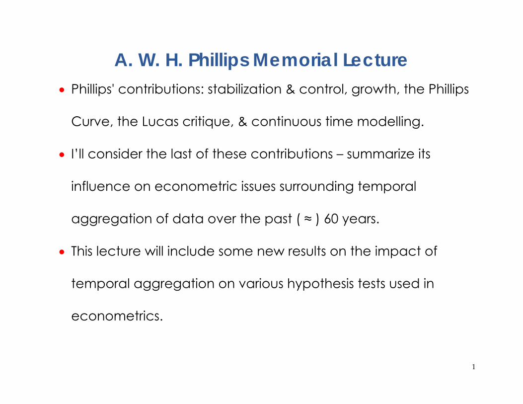
A. W. H. Phillips Memorial Lecture Phillips' contributions: stabilization & control, growth, the Phillips

Curve, the Lucas critique, & continuous time modelling.

I’ll consider the last of these contributions – summarize its

influence on econometric issues surrounding temporal

aggregation of data over the past ( ≈ ) 60 years.

This lecture will include some new results on the impact of

temporal aggregation on various hypothesis tests used in

econometrics.

 

2  

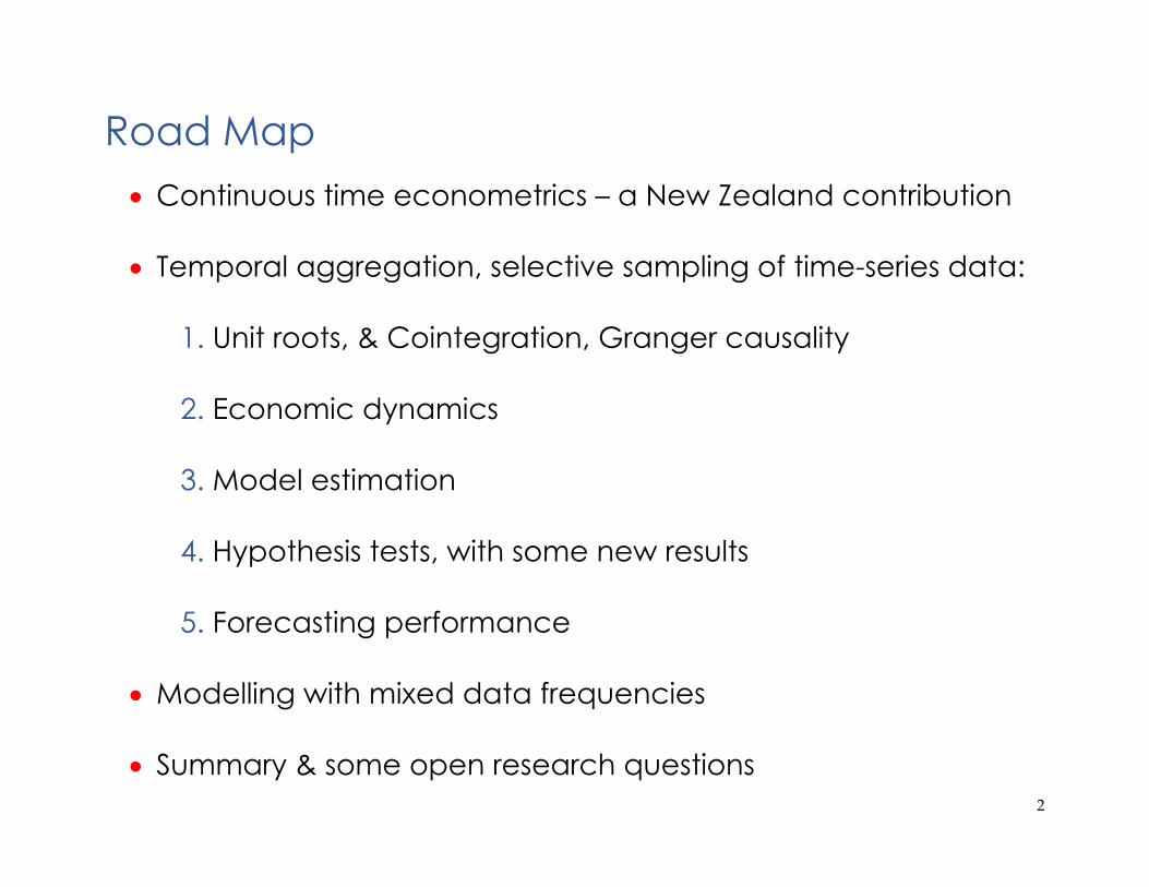
Road Map Continuous time econometrics – a New Zealand contribution

Temporal aggregation, selective sampling of time-series data:

1. Unit roots, & Cointegration, Granger causality

2. Economic dynamics

3. Model estimation

4. Hypothesis tests, with some new results

5. Forecasting performance

Modelling with mixed data frequencies

Summary & some open research questions

 

3  

Bill Phillips & Continuous-Time Modelling

Alban William Housego (Bill) Phillips (1914 – 1975)

 

4  

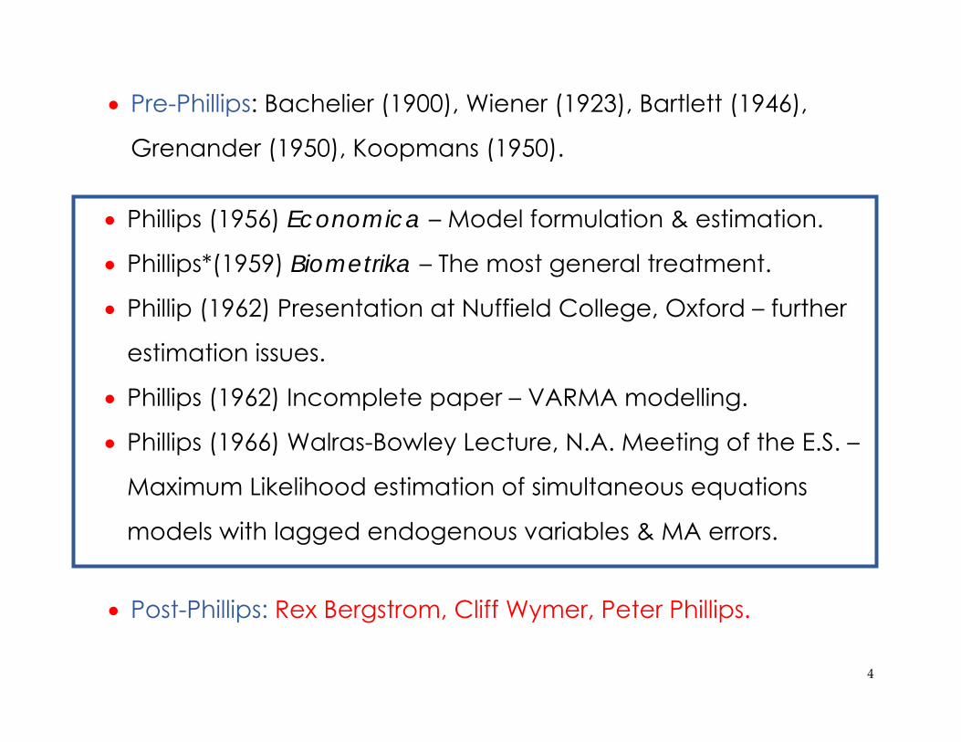
Pre-Phillips: Bachelier (1900), Wiener (1923), Bartlett (1946),

Grenander (1950), Koopmans (1950).

Post-Phillips: Rex Bergstrom, Cliff Wymer, Peter Phillips.

Phillips (1956) Economica – Model formulation & estimation.

Phillips*(1959) Biometrika – The most general treatment.

Phillip (1962) Presentation at Nuffield College, Oxford – further

estimation issues.

Phillips (1962) Incomplete paper – VARMA modelling.

Phillips (1966) Walras-Bowley Lecture, N.A. Meeting of the E.S. –

Maximum Likelihood estimation of simultaneous equations

models with lagged endogenous variables & MA errors.

 

5  

 

6  

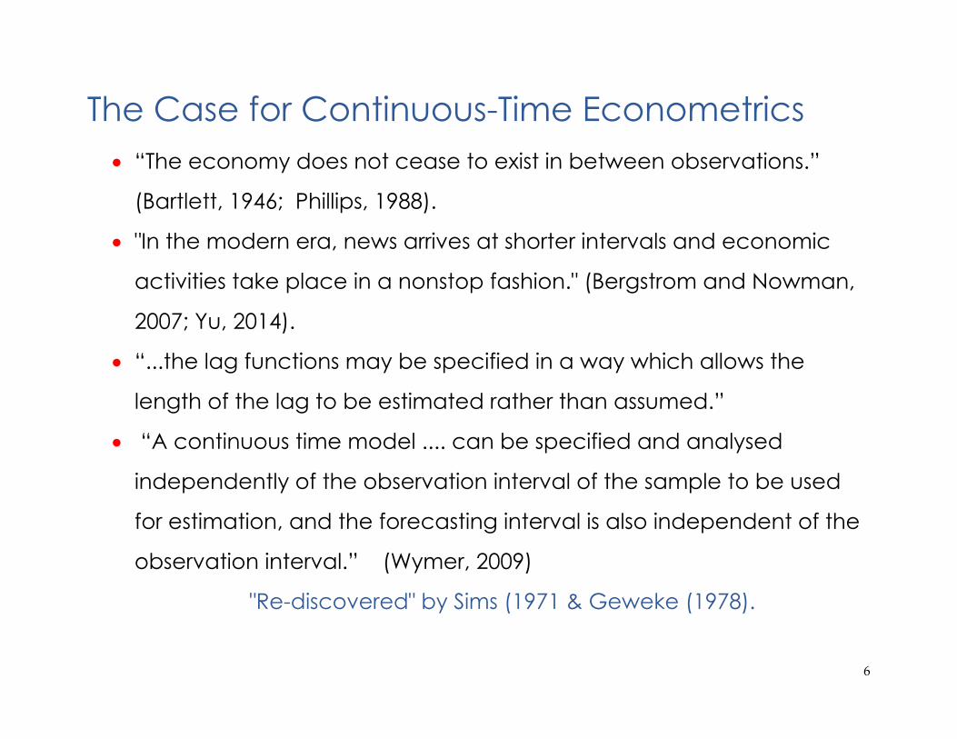
The Case for Continuous-Time Econometrics “The economy does not cease to exist in between observations.”

(Bartlett, 1946; Phillips, 1988).

"In the modern era, news arrives at shorter intervals and economic

activities take place in a nonstop fashion." (Bergstrom and Nowman,

2007; Yu, 2014).

“...the lag functions may be specified in a way which allows the

length of the lag to be estimated rather than assumed.”

“A continuous time model .... can be specified and analysed

independently of the observation interval of the sample to be used

for estimation, and the forecasting interval is also independent of the

observation interval.” (Wymer, 2009)

"Re-discovered" by Sims (1971 & Geweke (1978).

 

7  

Some Basic Results See Bergstrom (1984).

Typical discrete-time SEM:

Γ ∑

; ; Σ

Lots of (identifying) restrictions on and the matrices.

Continuous time: , … , ; , … , .

Stock variable - ; etc.

Flow variable - ; etc.

 

8  

Continuous-time system. For simplicity, if no exogenous

variables in the model:

Then there is an exact discrete representation of the

continuous-time model:

; ;

 

9  

Lagged values of all of the variables in the model appear in all

of the equations, and errors follow a vector MA process. It’s a

VARMA model, with particular restrictions on parameters.

The form of the VARMA model doesn’t depend on the

observation period – only on the form of the continuous-time

system.

Use FIML estimation to get asymptotically efficient, & super-

consistent, estimates of . Pretty challenging in 1956!

Notice that Phillips’ work really made the case for (restricted)

VARMA(X) modelling. Well ahead of its time.

 

10  

Temporal Aggregation

This will be main focus in this lecture.

Flow variables – monthly to quarterly; quarterly to annual, etc.

Summing data over several periods before using them.

Rather analogous to the shift from Continuous time to Discrete

time - integrating the data.

So, expect to encounter some similar modelling & inferential

issues.

These are driven largely by MA effects caused by aggregation.

 

11  

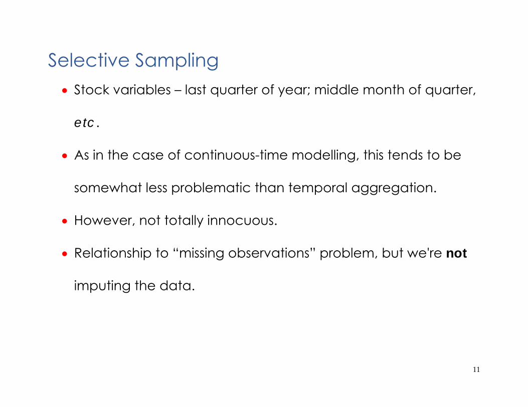
Selective Sampling Stock variables – last quarter of year; middle month of quarter,

etc.

As in the case of continuous-time modelling, this tends to be

somewhat less problematic than temporal aggregation.

However, not totally innocuous.

Relationship to “missing observations” problem, but we're not

imputing the data.

 

12  

Some Early Contributions Theil (1954), Nerlove (1959), Working (1960), Ironmonger (1959),

Mundlak (1961), Telser (1967), Engle (1969, 1970), Moriguchi

(1970), Zellner & Montmarquette (1971).

Temporal aggregation more of a problem for distributed lag,

and dynamic, models than for static models.

The long-run properties of a model are largely unaffected by

temporal aggregation, but the short-run properties can be very

sensitive.

 

13  

The BIG Picture Does the specification of the model suit the form of the data?

Analogy with non-stationary time-series.

Features of data have implications for modelling, inference.

N-S T-S: Spurious regressions; Unbalanced regressions; ECM,

cointegration; implications for estimation, hypothesis testing

& forecasting. Non-standard asymptotics.

Aggregation: Alters many characteristics of time-series such as model dynamics, lag relationships; can alter causality, non-linearities; implications for estimation, hypothesis testing & forecasting. Lose asymptotic normality. 

 

14  

Implications for Time-Series Properties Spectral shape Granger (1966)

 

Granger & Mortenstern (1963), Hatanaka (1963), Medel (2014).

Implications for modelling – e.g., DSGE models – Sala (2014).

Periodogram relatively invariant to temporal aggregation or

selective sampling, and to length of sample.

N.Z. merchandise imports (c.i.f.), 1984 – 2014:

 

15  

 

16  

 

17  

 

18  

White noise data Aggregation using m observations introduces MA(m-1) effect

(m = 3 ; monthly to quarterly)

~ . . . 0,

; 1

Y follows a non-invertible MA(2) process.

Fails conditions: 1 ; 1 ; | | 1

Implications for MLE & testing,

 

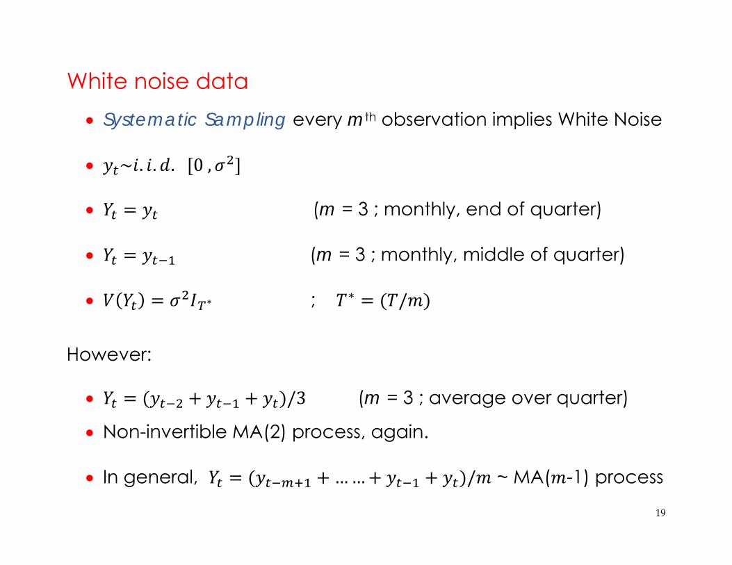
19  

White noise data Systematic Sampling every mth observation implies White Noise

~ . . . 0,

(m = 3 ; monthly, end of quarter)

(m = 3 ; monthly, middle of quarter)

∗ ; ∗ /

However:

/3 (m = 3 ; average over quarter)

Non-invertible MA(2) process, again.

In general, …… / ~ MA( -1) process

 

20  

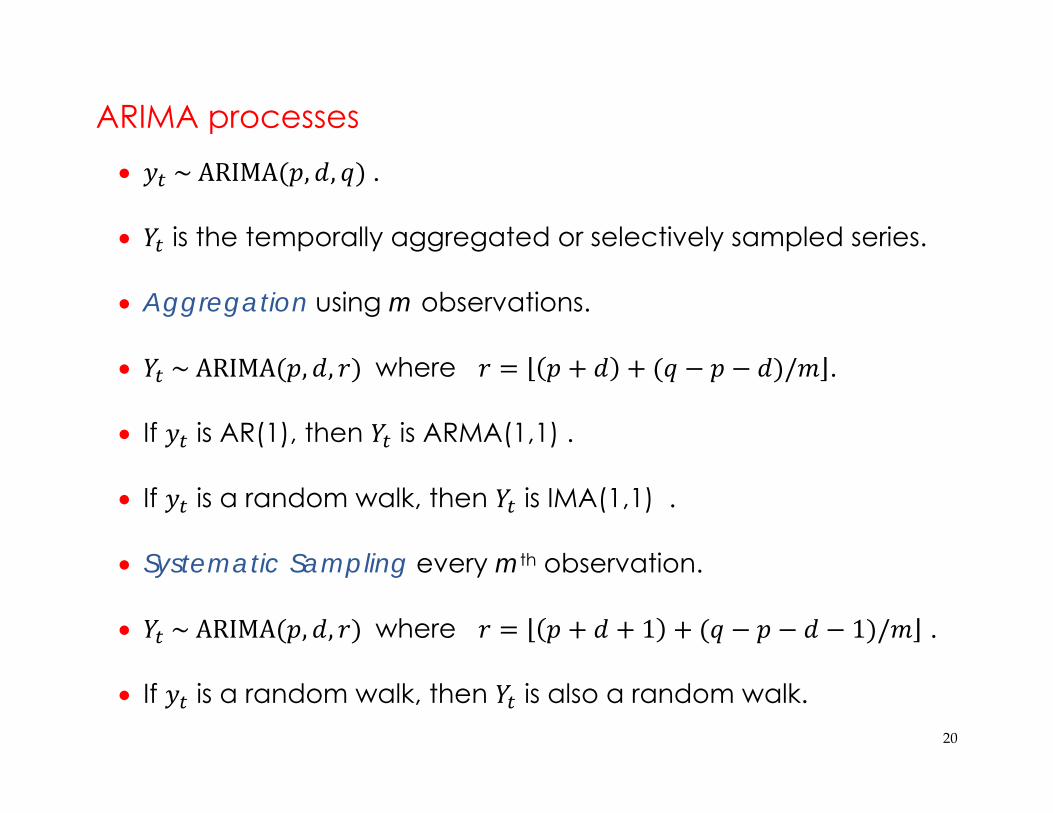
ARIMA processes ~ARIMA , , .

is the temporally aggregated or selectively sampled series.

Aggregation using m observations.

~ARIMA , , where / .

If is AR(1), then is ARMA(1,1) .

If is a random walk, then is IMA(1,1) .

Systematic Sampling every mth observation.

~ARIMA , , where 1 1 / .

If is a random walk, then is also a random walk.

 

21  

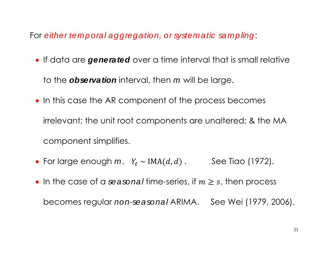
For either temporal aggregation, or systematic sampling:

If data are generated over a time interval that is small relative

to the observation interval, then m will be large.

In this case the AR component of the process becomes

irrelevant; the unit root components are unaltered; & the MA

component simplifies.

For large enough m, ~IMA , . See Tiao (1972).

In the case of a seasonal time-series, if , then process

becomes regular non-seasonal ARIMA. See Wei (1979, 2006).

 

22  

Unit Roots and Cointegration

Unit roots

Integrated time-series remain integrated under temporal

aggregation. See Lütkepohl (1987), Marcellino (1999).

~ 1 ⇒ ≡ ~ 0

⇒ ≡ ∑ ∑

+……+( )

⋯… ~ 0

⇒ ~ 1 .

 

23  

However, what about tests for stationarity/non-stationarity?

Pierce and Snell (1995):

; ~ ARMA( , ) ; and finite

: 1 vs. : / ; 0

(Sequence of local alternatives.)

Temporal aggregation or selective sampling; interval = .

ADF, PP, Hall-IV, tests, etc. (Similarly for KPSS, etc.)

“Any test that is asymptotically independent of nuisance parameters under both H0 and HA has a limiting distribution under both H0 and HA that is independent of .”

 

24  

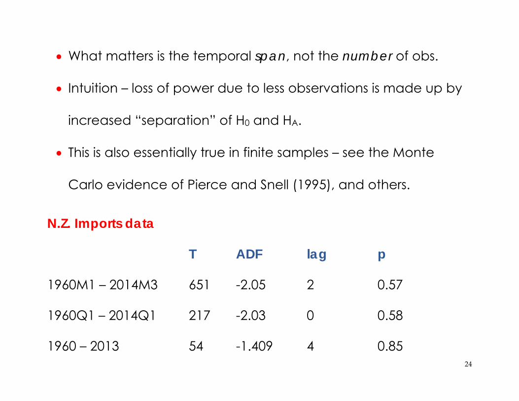
What matters is the temporal span, not the number of obs.

Intuition – loss of power due to less observations is made up by

increased “separation” of H0 and HA.

This is also essentially true in finite samples – see the Monte

Carlo evidence of Pierce and Snell (1995), and others.

N.Z. Imports data

T ADF lag p

1960M1 – 2014M3 651 -2.05 2 0.57

1960Q1 – 2014Q1 217 -2.03 0 0.58

1960 – 2013 54 -1.409 4 0.85

 

25  

Cointegration

If & are cointgrated, so are & (Granger, 1988).

~ 1 and ~ 1

There exists a unique such that ≡ ~ 0 .

⇒ ≡ ∑ ∑

+……+( )

. . … ~ 0

⇒ and are also cointegrated.

 

26  

Cointegration implies existence of an ECM for & of form:

Δ Δ ; Δ

Δ Δ ; Δ

and at least one of and is non-zero.

Δ ≡ ∑ ∑

Δ Δ ⋯ Δ

Δ ; Δ ⋯

Δ ; Δ

Δ ; Δ

 

27  

So, there must also be an ECM for and , but its lag

structure may be different from that for and

Recall “Early Contributions”.

The results of Pierce and Snell also apply to tests of

cointegration – e.g., Engle-Granger, Johansen.

What matters is the span of the sample, not the sample size.

Marcellino (1996): If ~ , then

1. The number & composition of the cointegrating vectors

are invariant to temporal aggregation.

2. Loadings of aggregated & diasggregated ECT’s are same.

 

28  

Granger Causality (One) Definition:

Let Ω , ; 0 and Ω′ , , ; 0 .

If there exists a 0 such that |Ω′ |Ω ,

then ⇒ with respect to Ω′ .

Usually test with 1 , using least squares optimal forecast .

Test of linear restrictions – special case – more later.

 

29  

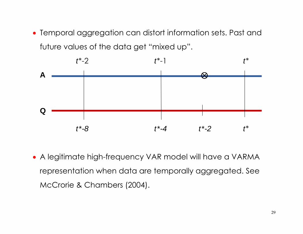
Temporal aggregation can distort information sets. Past and

future values of the data get “mixed up”.

t*-2 t*-1 t*

A

Q

t*-8 t*-4 t*-2 t*

A legitimate high-frequency VAR model will have a VARMA

representation when data are temporally aggregated. See

McCrorie & Chambers (2004).

                    

                    

⊗

 

30  

In the case of temporal aggregation: 1. If ⇏ , then ⇏ . 2. If ⟹ or ⟹ , then we can find ⟺ ;

or ⇏ ; and/or ⇏ .

3. If ⟺ , then we can find only ⟹ ; or vice versa.

See Sims (1971), Wei (1982), Christiano & Eichenbaum

(1987), Marcellino (1999), Gulasekaran & Abeysinghe

(2002), Breitung and Swanson (2002).

Same issues arise if data are non-stationary, and/or seasonal.

See Gulasekaran & Abeysinghe (2002).

 

31  

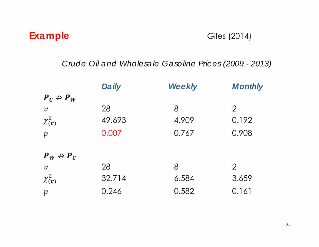
Example Giles (2014)

Crude Oil and Wholesale Gasoline Prices (2009 - 2013)

Daily Weekly Monthly ⇏

28 8 2 49.693 4.909 0.192

0.007 0.767 0.908

⇏ 28 8 2

32.714 6.584 3.659 0.246 0.582 0.161

 

32  

Granger-causality testing has been extended to the

continuous-time case. See Harvey & Stock (1989), Hansen &

Sargent (1991), and McCrorie & Chambers (2004).

Empirical example given by McCrorie & Chambers –

Money ⟹Income ? Monthly U.S. data, 1960M1 – 2001M12.

Continuous-time; MA(3) Discrete Monthly : ⇏

LRT 34.701 10.761

2 12

0.000 0.549

 

33  

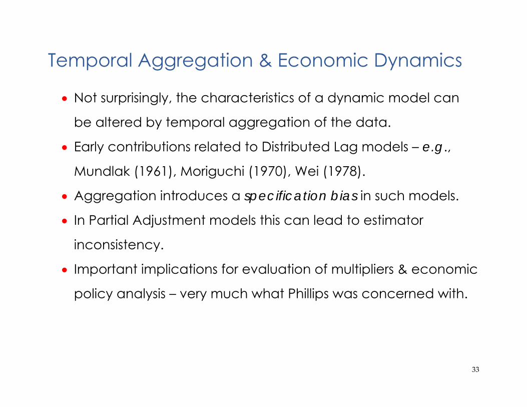
Temporal Aggregation & Economic Dynamics

Not surprisingly, the characteristics of a dynamic model can

be altered by temporal aggregation of the data.

Early contributions related to Distributed Lag models – e.g.,

Mundlak (1961), Moriguchi (1970), Wei (1978).

Aggregation introduces a specification bias in such models.

In Partial Adjustment models this can lead to estimator

inconsistency.

Important implications for evaluation of multipliers & economic

policy analysis – very much what Phillips was concerned with.

 

34  

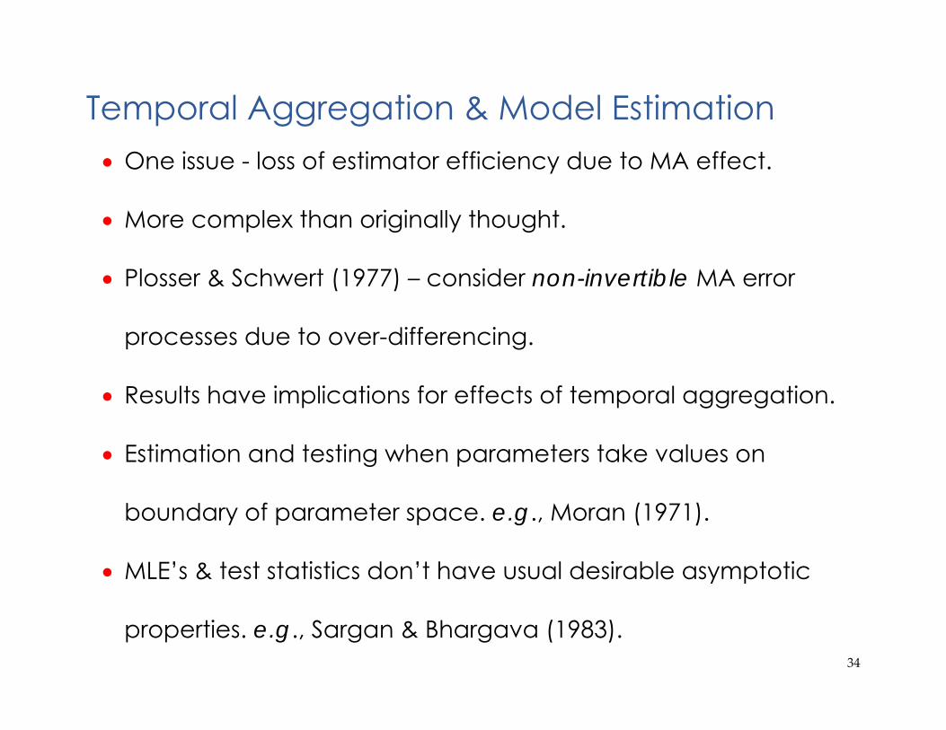
Temporal Aggregation & Model Estimation One issue - loss of estimator efficiency due to MA effect.

More complex than originally thought.

Plosser & Schwert (1977) – consider non-invertible MA error

processes due to over-differencing.

Results have implications for effects of temporal aggregation.

Estimation and testing when parameters take values on

boundary of parameter space. e.g., Moran (1971).

MLE’s & test statistics don’t have usual desirable asymptotic

properties. e.g., Sargan & Bhargava (1983).

 

35  

Monte Carlo experiment

Replications = 20,000

DGP – linear model with MA(2) errors

MLE – allowing for MA(2) errors

True parameter value = 1.0

 

36  

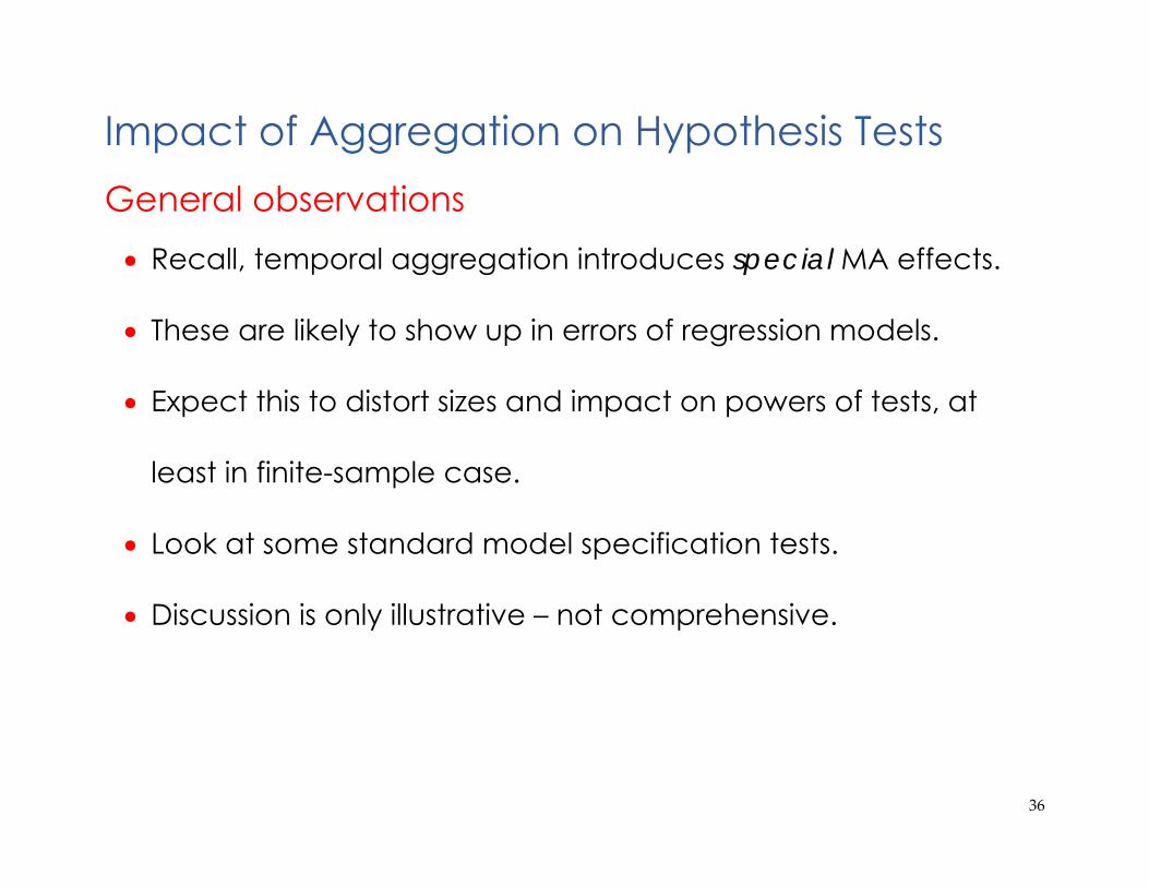
Impact of Aggregation on Hypothesis Tests General observations Recall, temporal aggregation introduces special MA effects.

These are likely to show up in errors of regression models.

Expect this to distort sizes and impact on powers of tests, at

least in finite-sample case.

Look at some standard model specification tests.

Discussion is only illustrative – not comprehensive.

 

37  

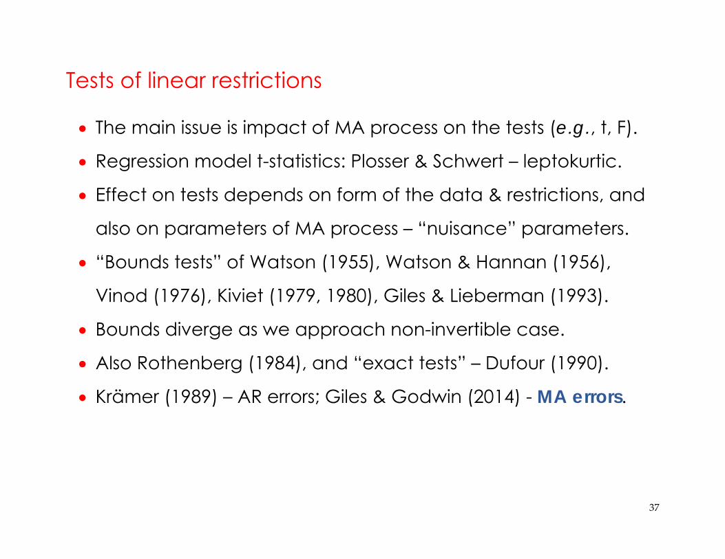
Tests of linear restrictions

The main issue is impact of MA process on the tests (e.g., t, F).

Regression model t-statistics: Plosser & Schwert – leptokurtic.

Effect on tests depends on form of the data & restrictions, and

also on parameters of MA process – “nuisance” parameters.

“Bounds tests” of Watson (1955), Watson & Hannan (1956),

Vinod (1976), Kiviet (1979, 1980), Giles & Lieberman (1993).

Bounds diverge as we approach non-invertible case.

Also Rothenberg (1984), and “exact tests” – Dufour (1990).

Krämer (1989) – AR errors; Giles & Godwin (2014) - MA errors.

 

38  

Example Giles & Godwin (2014)

; ~ . . . 0, 1

0.1 0,1

; 3

: 0 vs. : 0

t-test is UMP

20,000 replications in MC experiment

 

39  

Actual sizes

* \ : 12 50 100 500 5000 5000

1% 3.1 8.7 8.8 8.7 9.9 24.9

(11.6) (4.6) (3.1) (1.9) (1.2) (3.4)

5% 10.5 16.6 17.2 16.9 17.1 31.8

(21.4) (11.2) (9.1) (6.9) (5.6) (9.8)

10% 17.2 22.6 23.3 22.9 22.9 35.9

(27.4) (17.0) (15.1) (12.4) (10.8) (15.9)

(Tests based on Newey-West std. errors) Results for 12

 

40  

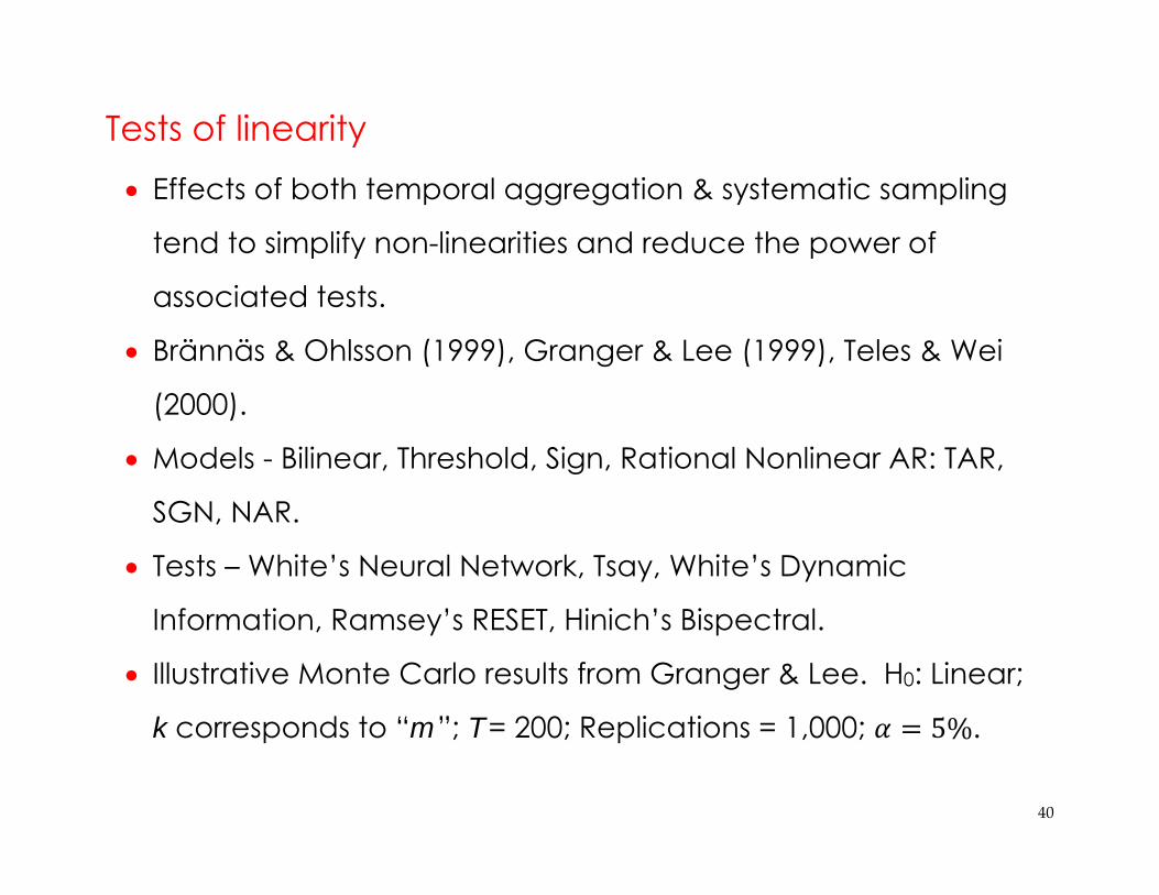
Tests of linearity Effects of both temporal aggregation & systematic sampling

tend to simplify non-linearities and reduce the power of

associated tests.

Brännäs & Ohlsson (1999), Granger & Lee (1999), Teles & Wei

(2000).

Models - Bilinear, Threshold, Sign, Rational Nonlinear AR: TAR,

SGN, NAR.

Tests – White’s Neural Network, Tsay, White’s Dynamic

Information, Ramsey’s RESET, Hinich’s Bispectral.

Illustrative Monte Carlo results from Granger & Lee. H0: Linear;

k corresponds to “m”; T = 200; Replications = 1,000; 5%.

 

41  

Rejection frequencies (i.e., powers)using simulated (asymptotic)

critical values.

 

42  

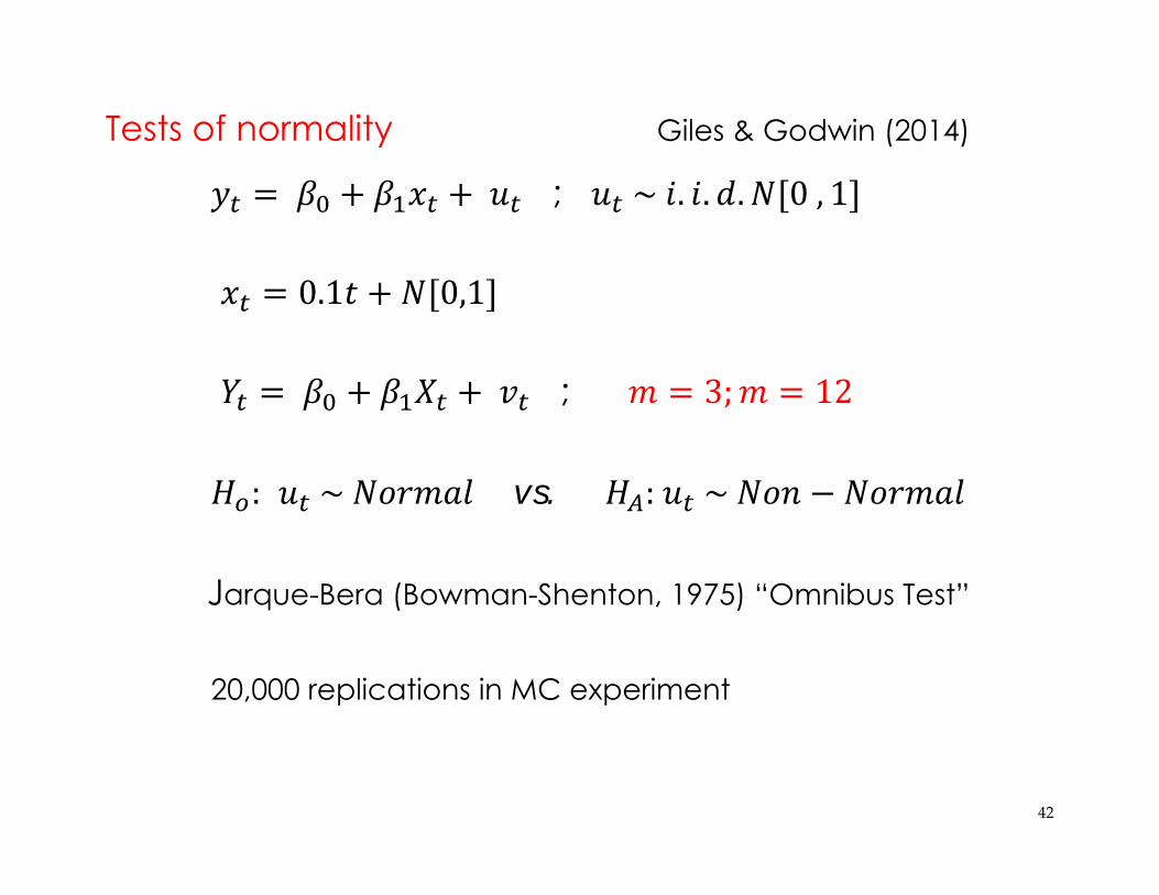
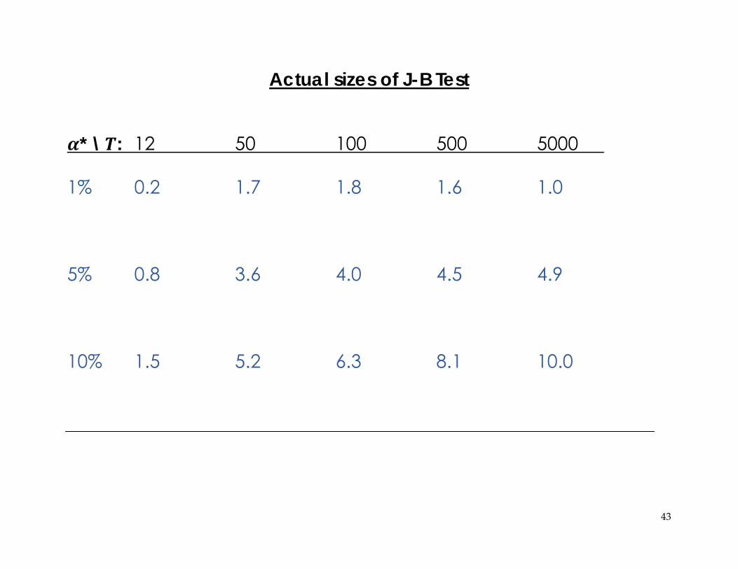
Tests of normality Giles & Godwin (2014)

; ~ . . . 0, 1

0.1 0,1

; 3; 12

: ~ vs. : ~

Jarque-Bera (Bowman-Shenton, 1975) “Omnibus Test”

20,000 replications in MC experiment

 

43  

Actual sizes of J-B Test

* \ : 12 50 100 500 5000

1% 0.2 1.7 1.8 1.6 1.0

5% 0.8 3.6 4.0 4.5 4.9

10% 1.5 5.2 6.3 8.1 10.0

 

44  

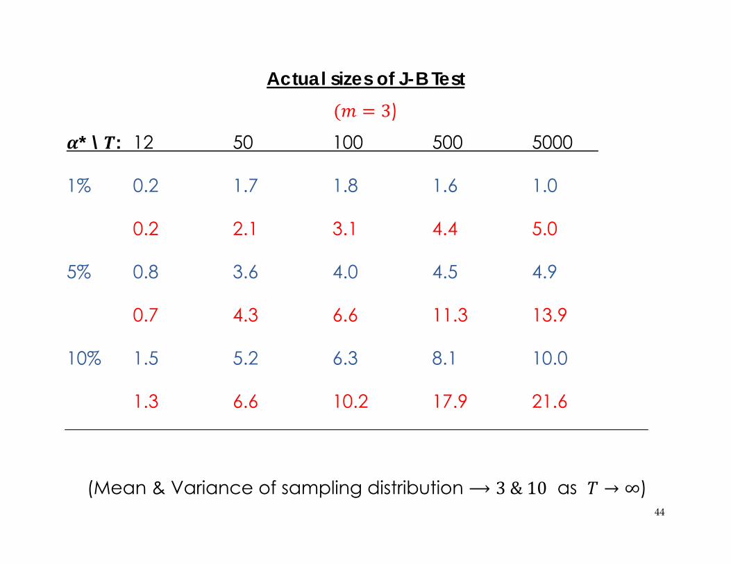
Actual sizes of J-B Test 3)

* \ : 12 50 100 500 5000

1% 0.2 1.7 1.8 1.6 1.0

0.2 2.1 3.1 4.4 5.0

5% 0.8 3.6 4.0 4.5 4.9

0.7 4.3 6.6 11.3 13.9

10% 1.5 5.2 6.3 8.1 10.0

1.3 6.6 10.2 17.9 21.6

(Mean & Variance of sampling distribution ⟶ 3&10 as → ∞)

 

45  

Powers of J-B Test ;

* \ : 12 25 50 100 250 500

1% 3.5 27.3 55.7 84.2 99.4 100

0.6 6.8 22.2 45.6 78.8 95.9

5% 7.3 33.9 63.1 88.8 99.8 100

1.4 11.1 29.0 53.5 88.4 97.6

10% 10.0 38.1 67.4 91.2 99.9 100

2.1 14.3 33.6 58.4 87.1 98.2

Test can be “biased” (even without aggregation)

 

46  

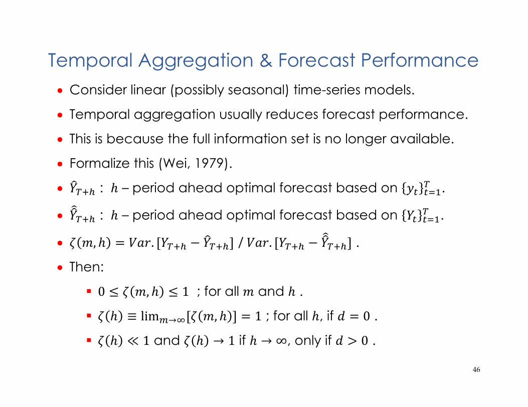
Temporal Aggregation & Forecast Performance Consider linear (possibly seasonal) time-series models.

Temporal aggregation usually reduces forecast performance.

This is because the full information set is no longer available.

Formalize this (Wei, 1979).

: – period ahead optimal forecast based on .

: – period ahead optimal forecast based on .

, . / . .

Then:

0 , 1 ; for all and .

≡ lim → , 1 ; for all , if 0 .

≪ 1 and → 1 if → ∞, only if 0 .

 

47  

Example (Anathanasopoulos et al., 2011) Tourism Forecasting With 366 Monthly Time-Series

Effects of Temporal Aggregation on Forecast Performance

(MAPE, %)

ETS ARIMA ForePro

Yearly 11.79 16.49 10.99 14.59 11.44 15.36

m = 4 10.32 14.32 9.94 13.98 9.95 14.48

m = 12 10.29 14.29 9.93 13.96 9.92 14.46

 

48  

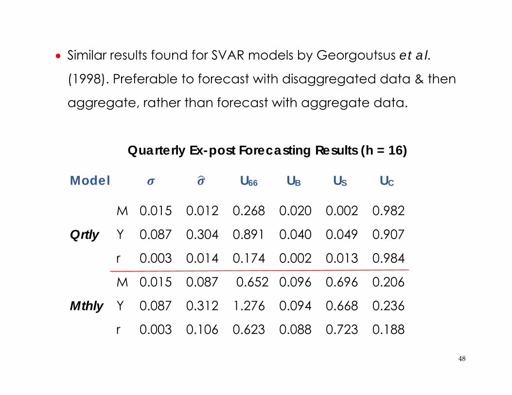
Similar results found for SVAR models by Georgoutsus et al.

(1998). Preferable to forecast with disaggregated data & then

aggregate, rather than forecast with aggregate data.

Quarterly Ex-post Forecasting Results (h = 16)

Model U66 UB US UC

M 0.015 0.012 0.268 0.020 0.002 0.982

Qrtly Y 0.087 0.304 0.891 0.040 0.049 0.907

r 0.003 0.014 0.174 0.002 0.013 0.984

M 0.015 0.087 0.652 0.096 0.696 0.206

Mthly Y 0.087 0.312 1.276 0.094 0.668 0.236

r 0.003 0.106 0.623 0.088 0.723 0.188

 

49  

MIDAS Modelling MIxed DAta Sampling regression models.

Eric Ghysels & co-authors.

Making the most of multi-frequency time-series data, without

resorting to imputation.

Avoids unnecessary temporal aggregation.

Easy to implement in R, or in MATLAB.

Lots of recent developments – 2013, 2014.

 

50  

Summary Bill Phillips pioneered continuous-time modelling in economics.

Many of the issues that his work revealed also arise when we

use discrete data that have been temporally aggregated.

Aggregation affects the time-series properties of our data due

to Moving-Average effects isolated by Phillips.

These, in turn, impact on virtually all of our estimators, tests,

forecasts. Asymptotics can become non-standard.

Important implications for policy analysis.

Don’t aggregate if you don’t have to!

 

51  

Some Open Research Questions “The topic of mixed frequency data, temporal aggregation

and linear interpolation is being researched again more

intensely in recent years ..…” Ghysels & Miller (2014)

Can we use tests of MA process non-invertibility to help assess

the magnitude of temporal aggregation “problems”?

Tests: Tanaka & Satchell (1989), Tanaka (1990), Larsson (2014).

What are the effects of temporal aggregation on various tests?

How far can we go with MIDAS modelling?

What are the gains of modelling in the frequency domain?

 

52  

Slides and Bibliography

davidegiles.com (“Downloads” ; “NZAE 2014”)

Contact Information

dgiles@uvic.ca davegiles.blogspot.com