Department of Aerospace Engineering - NASA · PDF fileDepartment of Aerospace Engineering ......
89
NASA CR 137942 Department of Aerospace Engineering University of Cincinnati AN INVESTIGATION OF VISCOUS LOSSES IN RADIAL INFLOW TURBINE NOZZLES BY I, KHALIL, W.TABAKOFF AND A.HAMED f(AsA-cn-137942) AN INVESTIGATION or VISCOUS LOSSES IN HADIAL INFLOW TU3EINE N77-17394 NOZZLES Interim Tieport (Cincinnati Univ.) 87 p HC A05VW A01 CSCL 20D K ___ 13 3/3!4 Unclas. l14S87 Supported by: NATIONAL AERONAUTICS AND SPACE ADMINISTRATIONEI6N Ames Research Center Contract No. NAS2-7850 RPRODUCED BY NATIONAL TECHNICAL INFORMATION SERVICE US DEPARTMENT OF COMMERCE SPRINGFIELD. VA.22161 https://ntrs.nasa.gov/search.jsp?R=19770010450 2018-05-11T01:04:48+00:00Z
-
Upload
truongnguyet -
Category
Documents
-
view
215 -
download
1
Transcript of Department of Aerospace Engineering - NASA · PDF fileDepartment of Aerospace Engineering ......

NASA CR 137942
Department of Aerospace Engineering
University of Cincinnati
AN INVESTIGATION OF VISCOUS LOSSES IN
RADIAL INFLOW TURBINE NOZZLES
BY
IKHALIL WTABAKOFF AND AHAMED
f(AsA-cn-137942) AN INVESTIGATION or VISCOUS LOSSES IN HADIAL INFLOW TU3EINE
N77-17394
NOZZLES Interim Tieport (Cincinnati Univ) 87 p HC A05VW A01 CSCL 20D
K ___ 13 334 Unclas l14S87
Supported by
NATIONAL AERONAUTICS AND SPACE ADMINISTRATIONEI6N
Ames Research Center
Contract No NAS2-7850
RPRODUCEDBY NATIONAL TECHNICAL INFORMATION SERVICE
US DEPARTMENTOF COMMERCE SPRINGFIELDVA22161
httpsntrsnasagovsearchjspR=19770010450 2018-05-11T010448+0000Z
N77-17394
An Investigation of Viscous Losses in Radial Inflow Turbine Nozzles
I Khalil et al
University of CincinnatiCincinnati Ohio
NOTICE
THIS DOCUMENT HAS BEEN REPRODUCED
FROM THE BEST COPY FURNISHED US BY
THE SPONSORING AGENCY ALTHOUGH IT
IS RECOGNIZED THAT CERTAIN PORTIONS
ARE ILLEGIBLE IT IS BEING RELEASED
IN THE INTEREST OF MAKING AVAILABLE
AS MUCH INFORMATION AS POSSIBLE
I Report No 2 Governrment Accession No Catalog No
NASA CR 137942
4 Title and Subtile 5 Repor Date
An Investigation of Vi-scous Losses in Radial 6 Performing Organization Code
Inflow Nozzles
7 Atuthor(s) 8 Pertorming Organization Report No
I Khalil W Tabakoff and A Hamed
10 Work Unit No
9 Perforning Organization Name and Address
Department of Aerospace Engineering amp Applied Mechanics of CincinnatiUniversity
Cincinnati Ohio 45221 NAS2-785013 Type of Report and Period Covered
12 Sponsoring Agency Name and Address Contractor ReportNational Aeronautics amp Space Admi-nistrationWashington DC 20546 and 14 Sponsoring Agency Code US Army Air Mobility Research amp Development LabMoffett Field Califorya 94035
15 Sjpolementary Notes
Interim Report Project Manager LTC Dwain Moenrmana US Army Air MobilityResearch and Development Laboratory Ames Research Center Moffett Fieldcalifornia 94035
16 Abstract
A theoretical model is developed to predict losses in radial inflowturnine nozzles The analysis is presented In two parts The first oneevaluates the losses which occur across tne vaned region of the nozzlewhile the second part deals with the losses which take place in the vaneless field It is concluded that the losses in a radial nozzle wouldnot be greatly affected by the addition of a large vaneless space
17 Key Words (Suggested by Author(s)) 18 Ostribution Statement
Tur-bomachanerv Losses Unclassified -unlimited
Radial Turbine
19 Security Ceasiof (or this report) 20 Security Clasaf (or this page) 21 No of Pages 22 -ice
Unclassified Unclassified 83
For sale by the National Technical Inrormation Service Soringrield Virginia 22161
NASA CR 137942
AN INVESTIGATION OP VISCOUS LOSSES IN
RADIAL INFLOW TURBINE NOZZLES
by
I Khalil W Tabakoff and A Hamed
Supported by
NATIONAL AERONAUTICS AND SPACE ADMINISTRATION
Ames Research Center
Contract No NAS2-7850
if
TABLE OF CONTENTS
Page
SUMMARY 1
INTRODUCTION 2
PART ONE FRICTION AND MIXING LOSSES IN THE VANED REGION 4
Analysis 4
Sudden Mixing Analysis 8
Results and Discussion i 10
PART TWO FRICTION LOSSES IN THE VANELESS FIELD 13
The Three Dimensional Flow In The End WallsBoundary Layer 14
Calculation Of The Main Flow Properties InThe Vaneless Field 17
Formulation Of Relations Describing TheVariation of Flow Properties Along The Flow Path 19
Procedure For The Numerical Solutions ofGoverning Equations 23
Evaluation of Loss Coefficients Across theVaneless Field 25
Results and Discussion 27
CONCLUSIONS 30
REFERENCES 31
NOMENCLATURE 33
FIGURES 36
APPENDIX A - Formulation of Relations Between IntegralQuantities and Boundary Layer CharacteristicParameters 67
SUMMARY
A theoretical model is developed to predict losses in radial
inflow turbine nozzles The analysis is presented in two parts
The first one evaluates the losses which occur across the vaned
region of the nozzle while the second part deals with the losses
which take place in the vaneless field
In the vaned region equations are derived to relate the
losses to the boundary layer characteristic parameters on the
vane surfaces and over the two end walls The effects of vanes
geometry flow conditions and boundary layer characteristic
parameters at exit from the nozzle channel on the level of
losses are investigated Results indicate that the portion of
the losses incurred due to the end walls boundary layer may be
significant especially when these boundary layers are characterized
by a strong cross flow component
In the vaneless field the governing equations for the flow
are formulated using the assumptions of the first order boundary
layer theory The viscous losses are evaluated through the
introduction of a wall shear stress that takes into account the
effects of the three dimensional end walls boundary layer The
resulting governing equations are solved numerically and the
effects of some operating conditions and the nozzle geometry are
studied
It is concluded that the losses in the vaneless region may
be looked at as a secondary factor in the determination of the
overall efficiency of the turbine nozzle assembly
1
INTRODUCTION
In recent studies dealing with the flow patterns in radial
inflow turbines the flow is assumed to be isentropic with
a viscous loss coefficient introduced to account for actual
flow effects The studies of Ref [ 2] were based on the
assumption that the viscous losses within the flow passages
are proportional to the average kinetic energy in the passage
A proportionality constant was chosen such that the viscous
losses matched the values determined from the experimental
results Other studies [3) estimate losses using approxishy
mations based upon flat plate or pipe-flow analogies Although
in the past approximate and semi-empirical solutions for the
losses have been adequate for engineering purposes the present
sophistication of fluid machinery demands a closer view of
the problem
The real flow in the radial type machines is very complex
because it is viscous unsteady and three dimensional An
insight into the real flow processes can be achieved by breaking
the complex flow pattern into several regions Existing flow
theories can then be used to obtain a solution to the flow
together with some reasonable simplifying assumptions in each
of these regions Following this approach and referring to
Figure 1 the flow field in a radial turbine nozzle can be
divided into the following subdomains
a The passage between the blades in which the flow
is partially guided
b The throat region where the flow is directed from
the closed channel conditions to the vane outlet
free conditions
c The region just at the exit of the channel which
will be referred to as the zone of rapid adjustment
In this region a considerable portion of the
overall stator losses take place
d The vaneless space region
In the present work a theoretical model is developed to
predict the losses in the flow regions mentioned above The
2
investigation is presented in two parts The first part deals
with the flow losses in the vaned regions and the second part
with the losses in vaneless field In the first part the
friction losses which result from the boundary layers developshy
ment along the vane surfaces and over the end walls are
considered Mixing losses due to the nonuniform flow
conditions at exit from the vaned region are also taken
into account The analysis establishes relations that provide
the description of the flow properties at the entrance to the
vaneless field in terms of the boundary layer characteristic
parameters over the flow surfaces From these relations
the various factors influencing the losses in the vaned region
are determined and their relative effects are evaluated
In the second part of this study the viscous flow in
the vaneless field is analyzed The influence of the three
dimensional end wall boundary layers on the steady nozzle flow
is taken into consideration The effect of the nozzle
geometry and the flow characteristics on the losses in the
vaneless region are determined
Under the stipulation of the developed model the overall
losses between the inlet of the radial nozzles and the impeller
periphery may be considered as the sum of friction and mixing
losses in the vaned region plus the friction losses in the
vaneless field For an actual expansion process the mechanism
of all these losses are coupled The model adopted however
provides a simple guide for better understanding and estimating
radial nozzles loss data
3
PART I
FRICTION AND MIXING LOSSES IN THE VANED REGION
ANALYSIS
The purpose of the radial turbine nozzles is to convert the
pressure energy into flow kinetics energy In the vaned region
a torgue is imposed on the flow by means of the vanes following
the scroll and hence the angular momentum of the fluid changes
more rapidly than in the vaneless field The design objective
remains the same however to achieve the highest possible
efficiency The thin untwisted vanes forming the nozzle channels
are arranged around the circumferential direction with equal
spacing and orientation (Fig 1) In order to maintain a
sufficiently high vane chord Reynolds number the length to
width ratio of the passages between the vanes ranges between
1 and 3 and the vanes aspect ratio is often less than 1
As the flow passes through the vaned region it suffers a
loss in total pressure and kinetic energy This may be attributed
to the decrease in the flow momentum within the boundary layers
which are developed over the flow surfaces and to their mixing
with the main flow It can be seen from Figure 2 which is taken
from Reference [4] that the magnitude and the direction of the
flow velocity as well as the other flow properties are nonuniform
in both the axial and the tangential directions at nozzle inlet
These nonuniform flow conditions which constitute an additional
source of the losses are caused by the three dimensional flow
behavior in the scroll
Another possible mechanism that contributes to the losses
is the secondary flow which tends to move the boundary layer
material across the channel from the pressure side of a vane to
the suction side of the adjacent vane as shown in Figure 3
To obtain an exact solution of the real flow in the vaned
region with all the aforementioned effects included would be
impractical These factors can be examined separately to
determine how they affect the losses in the radial turbines
The work presented here is a study of the losses which result
from boundary layer development along the vanes surfaces and
over the end walls
4
Referring to Figure 1 the total pressure of the flow entering
the nozzle at radius ro is Pto As it leaves the nozzle at rl
there is a variation in the flow properties in both the circumfershy
ential and the axial directions due to the axial directions due
to the boundary layer development over the end walls and the vane
surfaces It is assumed that due to the mixing effects the
properties of the air stream are homogeneous at station 2 downshy
stream from the vanes exit The loss coefficients expressed
in terms of the total pressures at stations 0 and 2 will hence
represent the overall losses across the vaned region resulting
from the friction and mixing mechanisms The pressure and enthalpy
loss coefficients are given respectively by the following
relations
-T- -t2-t (PtoPt 2 ) 1 1 7_7D(Y-)Y
1-p2Pto (P toP2) ( -1 shy- - -11
In order to determine these coefficients in terms of the main
flow properties and the boundary layer parameters at station 1
the equations governing the flow motion between stations I and 2
are derived in the following sections
The Governing Equations
Consider a control volume with an axial depth 2b equal to
the nozzle depth that extends circumferentially between two
consecutive mid-channel stream surfaces as shown in Figure 4
The equations of conservation of mass energy angular momentum
and linear momentum in the Y-Y direction are written under the
following assumptions
a The total temperature is constant during the expansion
and the mixing processes
b The static pressure is independent of z and S at
station 1
c The flow pattern is similar in all the flow channels
between two neighboring vanes of angular spacing
equal to 2rZ
The Conservation of Mass
For steady flow conditions the following continuity equashy
tion applies for the control volume of Figure 4
5
+b +iZ +b +rZ I I (pVrcos) 1 dedz = f f P2V2r2cosa 2dedz (2) -b -rZ -b -nZ
If the left hand side of the above equation is expressed in terms
of the boundary layer characteristic parameters at station 1
by using equation (A24) of Appendix A the following relation
is obtained
(pV)1 rlcosa 1 [l-6 -6te-Ae = P2V2r2cosa 2 (3)1
In the above equation the subscript -1 refers to the conditions
outside the boundary layer regions at exit from the nozzle
channels a1 is the angle between the velocity vector and the
inward radial direction amp is the total nondimensional disshy
placement thickness over the vane surfaces at station 1 and
ate denotes the trailing edge blocking factor 8 is the
streamwise total nondimensional momentum thickness over the two
end walls at station 1 and X is a parameter given by Equation
(A23) that depends on the end wall boundary layer profiles
Conservation of Angular Momentum
If the equation of conservation of angular momentumn is
written for the same control volume the following expression
is obtained
+b +Z 2 2 +b +Z 2 2 I I P2 r2V 2 cosa 2sina 2 dedz - I I (pr V cosasina)Idedz = 0 -b -rZ -b -iZ (4)
Using Equation (A23) of Appendix A Equation (3) can be written
as follows
2 2 2 2 P2V2cosa 2sina2 r2-(PV )ICosalsin 1 r1El-amp _Stee -ne = 0 (5)
In the above equation 0 is the total nondimensional momentum
thickness over the vane surfaces and r is a pararcter to be
determined from the end wall boundary layer velocity profile
at station 1 using Eq (A31)
6
Conservation of Linear Momentum
Referring to Fig 4 the momentum equation in the Y--Y
direction is expressed as follows
+Ib -4-Z 2- f f [pV cosa r cos(a+O)] 1 dadz
-b -wZ
+b +iZ 2+ I I P2V2r2cosa2 cos(a 2-0+8)dedz
-b -irZ
+b +7Z +b +rZ- I I plrlcosededz - f f P2r2cos(a-e)dedz + Q + C-b -Z -b -rZ (6)
The first and second terms in the right hand side of Equation (6)
represent the component of pressure forces acting on the
surfaces CD and FE of Fig 4 in the Y-Y direction The next
term Q is the resultant of the pressure forces on the two
mid channel stream surface CE and DF in the same direction
The contribution of the body forces is represented by C and the
flow turning angle is equal to a When the first term on the left
hand side of Equation (6) is expressed in terms of boundary
layer characteristic parameters according to Equation (A41)
Equation (6) reduces to
2 rCos sin1-(pV2)Cs~a- Cos2 a Z--r202 V2 r20osa2 cos(ct2-$)sin - -(V) shy22V2 2 coa2 2w
sin z- r)-(S + te + e ) cos -
= 2plr1 sin 7 - 2P2r 2 cosa sin 1 + + + (7)-f z 22Z 2b 2b 2b
where r is a parameter that depends on the end wall boundarylayer profiles as given by Eq (A42)
7
The Energy Equation
Assuming no heat or work exchange between the flow in the
control volume and the surroundings and using the equation of
state for a perfect gas we obtain
(Pt) 1 t2l t2(Pt)_1 Pt2
1
Where the subscript t refers to the total conditions Assuming
the viscosity effects to be negligible in the free stream
between stations 0 and 1 Ptl will be equal to Prto and the
energy equation can be written as follows
(Pt Pto (9)T 2 Pt2
Equations (3) (5) (7) and (9) will be used to calculate
flow properties at station 2 in terms of the free stream and theboundary layer characteristic parameters at station 1 In order
to carry out a solution the radius r2 at which complete mixing
has occurred is to be known Moreover the detailed flow
conditions within the control volume are also needed in order
to evaluate the quantities P Q and the angle 8 in Equation (7)
SUDDEN MIXING ANALYSIS
The results obtained from the experimental investigation
of Ref [4] indicate that the nozzle wakes almost disappear
near the zone of rapid adjustment which is shown in Fig 1
Assuming complete mixing to occur at a radius r2 which is very
close to r1 is therefore an authentic model of reality
For the limiting case of r2 approaching rl the flowdeflection angle the contributions of pressure forces acting
on the mid-channel stream surfaces CE DF as well as the body
forces in the Y-Y direction will diminish Consequently theterms Q C and the angle 8 in Equation (7) will tend to zero
and the governing equations are simplified to the following
form
8
Pt2 cosa1 1 M1 (1-6 -6te-A8 (
to cOSc 2 P2 N2
M2 sinct2 [l-s 6te- X J = 1 sinal[l-6 -6e- -ne 1 ()
2 2 e ( +Ste) ] i - 2
M2 Cosa M1 CosEl - - + + + - I- 2tan 2y y+ 1
Z
M rn 2 2 y+l y- 2 M1 cosll-6 -t- )M 2 cs2 + - y+2- 2
(12)
where
V1 V2M1 (V-crl 1 P 1 M2( r Vc2 Ptr t= M = 2 r 1 t or2 t
(13)
Equations (11) and (12) can be solved simultaneously to determine
the axisymmetric flow properties M2 and a2 providing that theflow conditions and the boundary layer characteristics are
defined at the nozzle exit Once M2 is obtained the density
ratio P2 could be calculated from the following identity
1 1 y-i M2y-i
(14)+-l 2
If a similar expression for p1 in terms of M1 is used togetherwith Equation (14) into Equation (10) the ratio between the
total pressures Pt2 and Pto is obtained These pressure-ratios
are substituted into Equation (1) to determine the overall losscoefficient across the nozzle vanes These loss coefficients-aill hence depend upon the nozzle geometry the flow conditions
MI al and the boundary layer characteristics 6
X and n at the nozzle channel exit
9
1
RESULTS AND DISCUSSION
The results of the present analysis show the effects of
variation in nozzle geometry flow conditions M1 a and the
boundary layer characteristics 6 8 r X and n on the
level of losses across the vaned region A series of figures
in which the variation of the loss coefficients Y with only
two of the afore mentioned variables are presented at specified
values for the rest of the parameters
Figures 5 6 and 7 represent the overall loss coefficient
and E at flow discharge angle a1 of 450 600 and 750 Each
figure demonstrates that the overall loss coefficients increase
with increased nondimensional vane surface boundary layer momentum
thickness a for different values of the streamwise nondimensional
momentum thickness of the end wall boundary layer 8 It can
also be seen from these figures that the losses decrease with
the decrease in the end wall momentum thickness 8 with the
minimum values corresponding to 8 = 0 This lower limit
represents the losses in a nozzle channel of infinite aspect
ratio The nondimensional momentum thicknesses 8 and 0 are
defined by Equations (A22) and (A27) and are both evaluated at
exit from the nozzle channels
Equation (A27) shows that the nondimensional momentum
thickness 8 is inversely proportional to the cosine of the
flow discharge angle aI For a specified value of the vane
surface boundary layer momentum thickness a will increase
with increased aI Figures 5 6 and 7 can therefore be used to
show that the losses increase with increased flow discharge
angles This effect becomes more significant at higher values
of a1 An accurate estimation of the exit flow angles is hence
essential for loss evaluation
Figure 8 shows the effect of the streamwise shape parameter
Hx on Y for the case of small crQss flowas t s olvibun
the Y is a weak function of Hx which is known not to exceod 2
for unseparated turbulent boundary layers [62 For all values
of a presented the loss coefficients were found to increase
not more than 5 for a corresponding increase in Hx from 12 to 2
10 -bpftDIBIL1TY OF THF
~ 1RTMM PAGE IS POOR-
Since the vane trailing edge thickness te is increased
when cooling of the radial turbine is considered it would be
desirable to examine the effect of te on the overall losses
in some detail This effect is investigated through the use
of the parameter t + + p- The results are presentede s pr21
in Figure 9 as the ratio between the loss coefficient Y at
a finite value of t to Y calculated for zero trailing edgee thickness Figure 9 shows that the increase in the losses can
be considerable for larger values of the trailing edge thickness
Under normal operating conditions corresponding to 6 = 002
and e = 0015 in a conventional turbine with trailing edge thickness parameter t +6 +6plvz of about 003 the
e s r trailing edge contributi6n to the losses is about 25 percent
If the parameter t +S +6 2 Z is increased to 007 thee s p r1
portion of the losses due to the finite trailing edge is
increased to 82 percent
The effect of compressibility on the overall loss coefshy
ficients are shown in Figures 10 and 11 It can be seen
from Figure 10 that the enthalpy loss coefficient remains
practically constant with increased free stream Mach number
for the different values of the boundary layer parameters
considered On the-other hand the overall total pressure
loss coefficient Y increases significantly with increased
Mach number Figure 11 Due to the large sensitivity of the
pressure loss coefficient to Mach number variations it is
recommended to use the overall enghalpy loss coefficient C
in describing the loss performance characteristics of the
radial turbine nozzles
The effects of the end wall boundary layer cross flamp on
the losses are shown in Figures 12 and 13 Figure- 12 illutrate
the variation of Y with 0 for the different end wall
velocity profiles A B C and D of Table A-i in Appendix A
Since it was found previously that the loss coefficients
are weak functions of Hx it may be concluded by examining
Figure 12 that the cross flow profile parameters K and L
(see Equation A9 and A10) have a significant effect on the
losses As an example for a value of the nondimensional
1
streamwise momentum thickness 8 of 003 a variation in the
magnitude of losses up to 25 can result by considering
different profiles
Figure 13 shows the contribution of the cross flow to
the losses which were calculated using the end wall velocity
profile B It is clear from the figure that the minimum
losses are obtained for the case of collateral end wall boundary
layers e = 0 The losses increase appreciably for strong
cross flow cases corresponding to higher values of s
12
PART II
FRICTION LOSSES IN THE VANELESS FIELD
The vaneless nozzle in a radial turbi-ne consists of a smooth
walled axisymmetric passage with radial or conical surfaces The
passage depth may change with radius but a little influence on
both the pressure and velocity distribution is noticed since the
angular component of the fluid momentum is predominant Basically
the flow in the vaneless nozzle can be treated as a vortex motion
except for the skin friction which acts upon the flow boundaries
In overcoming the resistance along its path the flow loses part of
its total pressure The pressure loss occurs at the expense of
both static and dynamic pressure (8]
Loss analysis for the turbine vaneless nozzle may be treated
using the same methods developed for the compressor vaneless
diffuser provided that the area changes as well as the flow
direction are taken into consideration Conventional flow
analyses for the vaneless diffuser [9 10 11] were based on the
assumption of one dimensional flow Total pressure losses were
determined using a constant friction coefficient In a recent
study Jansen [12] arrived at a more accurate evaluation for the
friction coefficient and its variation along the flow path
His analysis however requires much more detailed knowledge of
the flow conditions than can actually be realized in practice
In the following study the governing equations for the flow
in the vaneless space are formulated using three dimensional end
wall boundary layer theory [6] The resulting differential equations
are solved numerically to obtain the flow properties within the
vaneless field The losses are evaluated taking into account both
the wall friction and the momentum flux changes due to velocityshy
profile variation along the flow path The effects of some
parameters representing the operating conditions and nozzle
geometry on the losses incurred within the vaneless field are
also investigated
13
THE THREE DIMENSIONAL FLOW IN THE END WALLS BOUNDARY LAYER
Flow Pattern
As the flow in the vaneless field proceeds towards theimpeller tip the main streamlines turn as shown in Fig 14
A balance is established in the main stream between the static
pressure gradients and the centrifugal forces caused by the flow
turning The unbalance between the externally imposed pressure
gradients and the centrifugal forces of low momentum end wallboundary layers produces an acceleration component normal to
the main stream direction in the boundary layer fluid
Consequently the velocity in end wall boundary layers is
different from the mainstream velocity V not only in magnitude
but also in direction The velocity profiles in this skewed
boundary layer is shown in Fig 15 Taylor [13) noticed that
the polar plot of the velocity vector in a skewed boundary layer
follows a triangular form such as shown in Fig 15 Thus
any analysis of such boundary layer is usually carried out using
different formulation in the inner and outer sublayers
The Inner Sublayer
Referring to Fig 15 the following linear relation between
the cross flow velocity component w and the streamwise velocity
component v holds good
w = v tan tmax (15)
The angle pmax in the last equation is invariant within the
collateral inner sublayer Accordingly it can be estimated
at the wall using the following relation
tan max Limit S (16)-- =
Since the skin friction is in the same direction as the velocity
vector at the wall therefore it will deviate by the angle
max from the main flow direction If the wall shear stress
and the friction coefficient are denoted by Tr0 and Cf respectively
14
and if their components in the main flow direction by -cx and
Cfx then
Cf = Cfx(l + C2 )12 (17)
where
T
Cf 1 2 (18)
and
T 2C = 1V (19)
Ludwieg and Tillman [14] deduced an accurate semi-empirical
expression for the wall friction of two dimensional flows in
the presence of favorable pressure gradients Johnston [61
showed that in a skewed boundary layer the relation of
Ref [141 can be used to determine the component of the skin
friction coefficient in the main flow direction according to
the following relation
-0268 Cfx = 0246[ExpC-l561 Atx)JRe (20)
where Hx is the streamwise shape factor and ROx is the
Reynolds number based on the streamwise momentum thickness
Referring to Fig 16 the components of shear stresses in
the tangential and the radial directions are
x6 = T0 sin( t-max) (21)
t= T0 max)a (22)Tr o cos(a -
When Equations (16) (17) and (18) are substituted in Equations
(21) and (22) the following relations are obtained
e 1 PV2Cf[Sin - pound cosc] (23)
15
1 pv2CfxECOS + e sina] (24)
In the above equations the values of a and s will depend
on the main flow variables The expressions which are used in
evaluating these parameters are given in the outer sublayer
analysis that follows
The Outer Sublayer
The two velocity components in the non-collateral cuter
sublayer namely the cross flow component w and the streamwise
component v are related by the following equation
w = A(V - v) (25)
The parameter A depends on the main flow turning angle (0)
which is shown in Fig 14 and is given by the followin expression
A =-2V 2 dS (25a)0 V
where V is the main flow velocity
The tangent s of the limiting angle m can be expressed
in terms of the parameter A and the streamwise friction coefficient
Cfx according to the analysis of Ref 16] as
+)14
- 01 + - 1 (25b)
fx
Equations (20) (25) and (25b) can be substituted into Equations
(23) and (24) to predict the variation of shear components t Tr
along the flow path in terms of main flow variables The details
of the computation procedure used for this prediction is
presented in the section dealing with the Numerical Solution of
the Governing Equations
16
CALCULATION OF THE MAIN FLOW PROPERTIES IN THE VANELESS FIELD
Analysis
The vaneless space geometry together with the velocity
triangles and the coordinate system are shown in Fig 17 It is
assumed that the flow enters the vaneless field at the radius
r2 in a steady uniform axisymmetric pattern with specified
flow conditions These inlet flow properties are determined
from the vanes friction and mixing loss analysis presented in
Part I of this study
As the flow passes through the vaneless field there will
be a variation in its properties in both radial and axial
directions The variation in the axial direction z results
from the development of boundary layer over the two end walls
The static pressure distribution and the radial and tangential
velocity components will be determined along the main flow path
using the assumptions of the first order boundary layer theory
An equivalent one dimensional flow will be considered in a
nozzle with an effective depth of 2be t which is equal to the
actual nozzle depth 2b minus the displacement thicknesses
of the two end wall boundary layers at any radius r (see
Fig 18) The components of the velocity V and the pressure
p of the flow passing through this equivalent nozzle vary
only along the radial direction and are independent of z and
e The total pressure loss due to friction will be calculated
using the values of Tr and T developed in the previous section
and given by Equations (23) and (24)
Equations of Motion
The control volume of Fig 19 will be used in the following
derivation The magnitude of the velocity V is considered to
increase as the flow proceeds inward in the vaneless nozzle
Furthermore the flow will be assumed to be steady and adiabatic
17
Conservation of Angular Momentum
Setting the net efflux of angular momentum through the
control volume equal to the external torque due to the shear
force in the tangential direction we obtain the following
relation
PbeV cosa (r V sina) = Ter (26)
Substituting for T from Equation (23) into Equation
(24) we get V cos__Vsin_ d CfXV2
Cosa V sina + V cosa - (V sina) = r[sina - scosal r dr 2be
(26a)
Conservation of Linear Momentum in Radial Direction
d PbeV2sin 2 a-PbeV Cosa -( CVcosa) = bedr (P)- 27)
The left hand side of the above equation is equal to the net
radial momentum flux The first two terms on the right hand
side are the radial components of the pressure forces and the
wall friction forces while the third term represents the
centrifugal forces
Substituting for Tr from Equation (24) into (27) and
rearranging we obtain
dp Cfx 2[s nsin2a 2d oe p dr 2be r-Vcsdr V r-V coscoa - _ V [Cosai + esinalshy
(27a)
Conservation of Mass
From continuity considerations the following differential
equation is obtained
18
I dp + 1 d(V cos) +1 1+ dbe
pdr V cos dr r bdrshye
Equation of State
The pressure density temperature relation for a perfect
gas is used in the following differential form
l dp 1 dp 1 dT (29)p dr p dr T Ur
Energy Equation
Since the total temperature remains constant during the
expansion process in the vaneless field the differential form
of the energy equation may be written as
M2d-y-l 2
1 dT _ M 1 dM2 (30) M2T dr 1 + yl 2 dr
M2 Which when combined with the definition of the Mach number
reduces to
1 dV2 1 2 1 d v 1- I I (30a)
M IdrY-l2V2 dr 2
Formulation of Relations Describing the Variation of Flow Properties Along the Flow Path
Equations (26) through (30) will be manipulated to obtain
the following relations which are used to calculate the pressure
Mach Number and the main flow angle
Pressure Distribution
Combining Equations (29) and (30a) the following relation
is obtainedp-i M2 2
1 dp 2 1 dMdp p dr p d-r 1+ X31M 2 d
2 M
Dividing Equation (27a) by V2cos2a and using the identity
pV2 = yp M2 (32)
gpRUCIBL1TY OF THE19 z POOR16gVOAL PLO
one gets an expression describing the variation of the tangential
velocity component with radius as
1 d 1 1 dp Cfx (cosa + ssin) tan2 a Cosa dr (V cosa) 2o2P - - 2e 2 ryMCos a e Cos as
(33)
Substituting for 1 do from Equation (31) C1osa r (V cosa)p dr
from Equation (33) into the continuity Equation (28) the
variation of pressure with radius is deduced as
1 dp M2 Cfx (cosa + Esina) sec2a p dr 2 2 [- 2 r
M -sec eO aoc
y- M2 2 db - 1 M 1 dM 1 e (34)
-1 2d2r Fbdr-
Mach Number Distribution
In order to obtain the variation of Mach number along the
flow path an additional equation relating the pressure in terms
of M and a is required This relation is obtained by combining
the equation of angular momentum (26a) with the equation of
linear momentum (27a)
1 1 dp Cfx 1 1 dV2 (35)22p dr 2b Cosa)c 2 v dr
Substituting Equations (30a) and (32) into the last equation
it reduces to
1 dp = yM2 -1 1 d2 Cfx (36)) M2 dr + 5ecoSaN-+ 12pd-r--2
Now eliminating dp between Equations (34) and (36) the
p dr
Mach number variation along the radius r is obtained from the
resultant expression
20
1 dM 1 ( 2 2 fx 2 be21M 1sect + C sec(M - tan2 a + Etana)+ e
M2 2 r 2beg d
(37)
Flow Direction
The differential equation of flow direction may be developed
using the following relation
tana = V sin (38)
V cosa
This last equation can be written in the following differential
form
I d(tana) _ 1 d(V sina) 1 d(V cosa) tan dr s dr V cosat r (38a)
Substituting Eq (26a) and (33) intoEquation (38a) the following
relation is obtained
2 21 d(tana) _ sec a 1 dp sec (39)
tana dr yW-2 p dr r
1
Substituting for from Equation (34) and rearranging the
equation describing the variation of flow direction with radius
takes the following form
M2d- -tana Cfx sec [ 2 an++ db er b [i +Cy-l)M stan+2dr M sec a e e -d shy
(40)
Nondimensional Form of the Governing Equations
Before solving the equations of motion they will first be
written in a nondimensional form The nozzle dimensions will be
normalized with respect to the inlet radius r2 and the pressures
with respect to the total inlet pressure Pt2 as follows
2bR -rep r B e P 2 F2 Pt2
271
Equations (34) (37) and (40) can therefore be written in
the following nondimensional form using the above expressions
yM2 2I dP _ s Cfx (cosa + Esin) sec aP dy 2 s e 2 B 2 r
(~ 1 2 1d(421+ Y- M 2 ) M-I Y- - N I
2
1 dM 1 +Y M2 [sec2 a Cfx 2_ 2 d-R M2 _ seci (yM2tana3Ba T-
M _ sec aciB-
(43)
and
M2dM -tan Cf seca 2 lYB
2 dR M2_ sec2aRBd (1 +(yl)M+ etan)+ -- (44)
Furthermore if the thicknesses of the boundary layers developed
over the two end walls are taken to be equal then B the depth
ratio and its derivative could be expressed as
B 2b 26 (-) ( 5 =--- - -2d r r2 dR dR
where S is the streamwise displacement thicknessx
22
PROCEDURE FOR THE NUMERICAL SOLUTION OF THE GOVERNING EQUATIONS
In order to determine the flow properties within the vaneless
field the system of nonlinear differential Equations (43) (44)
and the algebraic Equations (20) (Z5a) and (25b) will be solved
A fourth order Runge-Kutta algorithm is used to solve the
simultaneous first order differential Equations (43) and (44)
The solution procedure consists of the following steps
1 The values of M a at the vaneless nozzle inlet are
assumed to be known from the analysis given in Part IdB
2 At any radius Ri f knowing Mi ai Cfx e B and -B
the increments in M and a over the radial distance (-AR) is
computed using the following recursion formula
N -M= _AR (K + 2K + 2K + K (46)i+1 -46 C= 2 23 + + +ai+l -ai = - A-R (KK 2KK 2KK KK (47)
1 1(12 213 1(4)
where
K= f(Ri M i ai)
KK 1 = g(Ri M i ai )
1AR K K
K2 i + --- ) (48)
KK 2 = g(R i AR M + K1 KK1
2- - L +-)
K3 f(Ri AR M 2 a+K21 2 i 2 i 2
KK 3 g(Ri AR +K2 KK23 2 i 2 i
23
K(4 f(R - AR Mi +K i + KK 3 )
KK4 = g(R i - AR M + K3 ai + KK 3 )
Where f represents and g d and are evaluated according dR U-R
to Equations C431 and C441 respectively using the known values ofCfx A e B and q- at the radius Ri
C f x ld R
3 At the end of the interval at the new-radial location
Ri - AR the quantities Cfx A E B and dB are evaluated using
Equations (20) (72ay and (25B respectively as will be explained
The streamwise friction coefficient Cfx is calculated according to
Equation (20) The boundary layer characteristic parameters ROx and
Hx in this equation can be evaluated using any method of
boundary layer solution In the present analysis the method of
Reference 15 was used for this purpose Integrating Equation (25b)
numerically starting from the vanalea nozzle fl-let until anshy
desired radius where the mean flow turning angle $ is known
gives the corresponding value of A at Ri1 These values of Cfx
and A are then substituted into Equation (25c) which is solved
for e using an iterative procedure
4 Refined values for Mi+ci+l at (Ri - ARI are obtained1
by substituting the arithmetic average between Ri and Ri+1 of the
variables Cf e B and - in the recursion formula (46) and (47)dR
5 The corresponding values for Cfx A e B - at R
are calculated as shown in Step 3 using the values of Mi+I
li+l obtained from Step 4
6 Steps 4 and 5 are repeated until successive values of the
computed flow variables are within the required accuracy in the
present study an accuracy of 0001 was maintained in the different
variables which was achieved after 2 iterations
7 The whole procedure (Steps 2 through 6) is repeated for
small values of (-AR) starting from the nozzle inlet up to the
impeller tip The numerical results reported herein were
calculated using radial increments AR equal to 001
24
EVALUATION OF LOSS COEFFICIENTS ACROSS THE VANELESS FIELD
Standard definitions of total pressure and enthalpy loss
coefficients in terms of the average pressures at inlet to and
exit from the vaneless region are adopted The total pressure
loss coefficient is given by
P t3
- t2 (49)
P 3
Pt2
while the enthalpy loss coefficient may be written as
Y-1Pt2 P t3t3 (50)(Pt2 -shy
P3
It is clear from the above two equations that the flow conditions
at station 3 the vaneless space exit have to be known in order to
calculate the loss coefficients
In the previous chapter it is explained how to determine
numerically the Mach number the flow angle and the effective
nozzle depth variations along the flow path Knowing the values
of these variables at the nozzle exit (-station 3) the static and
total pressures P3 and Pt3 are computed using the equations
derived below
The conservation of mass between the vaneless diffuser inlet
and exit is expressed as
P2V2cosa 2r2b2 = P3V3cosa 3r3be3 (51)
where 2b is the effective depth of the nozzle at station3
If the definition of Mach number and the equation of state
are substituted into the above Equation (51) the following
expression for p3P2 is obtained
25
P b2 r2 Cosa2 M2 I + 1-__ M2p3 2 2_ c 2 2
(52)2 bre r3 cosa3 M3 1 + yiM2
3 2 31
The total pressure at the vaneless space exit Pt3 is then
determined using the following relation
Pt3 P3 1 2 3 T-Pt2 =P 1 + y-- M2 (53)Pt2 P22 2
Equations (52) and (53) are sufficient to determine the loss
coefficients Y and provided that the inlet flow conditions to
the vaneless space are specified
26
RESULTS AND DISCUSSION
The numerical examples worked out using the present method of
analysis are presented in two groups In the first group the
effects of inlet flow conditions on the flow behavior and losses
in the vaneless field are investigated The second set of
results illustrate the influence of changing the end wall spacing
on the same flow parameters
1 Effects of Inlet Flow Conditions
The effect of two inlet flow parameters namely the Mach number
and the flow angle on the vaneless nozzle performance are considered
first Computations were carried out with an inlet Mach number of
08 and different inlet flow angles a2 the corresponding results
are shown in Figures 20 to Z2 On the other hand the data obtained
with different Mach numbers for a constant inlet flow angle of 70
are presented in Figures 23 to 25 The geometrical end wall spacing
2b and the inlet radius to the vaneless field r2 for this first
set of results were chosen to be 0339 and 393 inches respectively
The total temperature was held constant throughout the flow at 20000R
The change in angular momentum ratio r3V3sin 3r2V2sina2
with the normalized radius R is shown in Figure20 for different
values of inlet flow angles a2 It can be seen that
increasing a2 causes a reduction in the angular momentum ratio
everywhere This effect becomes particularly predominant at
high values of inlet flow angles For example at a normalized
radius of 09 the angular momentum ratio changes from 0992 to
0987 corresponding to an increase in a2 from 600 to 700
Meanwhile a further increase in a2 from 700 to 800 results in
a reduction of the same parameter from 0987 to 09732 2The radial variations of the ratio M3M2 are shown in
Figure 21 for three different values of inlet flow angle It can
be seen from the figure that increasing a2 reduces M3M 2 at each
radius This is a consequence of the larger reduction in the
tangential velocity component due to viscosity an influence
that dominates the augmentation in the smaller radial velocity
component It can also be concluded that for all the values of a2thrti M2 2
the ratio 3M2 increases as the flow proceeds inwards Thich is
anticipated
27
The variation in the pressure loss coefficient Y and
enthalpy loss coefficient C are shown in Figures 22a and 22b
respectively It is clear that both coefficients increase with
increased inlet flow angle a2 at every radial location If
the results of Figure 22 are compared with those obtained in
Part 1 it can be concluded that even for the largest values of
a2 the loss coefficients in the vaneless field are extremely
low as compared to the losses in the vaned region For example
the pressure loss coefficient of Figure 22b is as low as 00125
at R = 090 for values of a2 and M2 of 600 and 08 respectively
On the other hand the pressure loss coefficient of Figure 8
is as high as 0107 under the same operating conditions
Briefly one can conclude that increasing the inlet flow
angle a2 results in a larger reduction in the total pressure
Mach number and angular momentum at nozzle exit This can be
attributed to the longer path that the flow has to take to reach
a certain radius if the inlet flow angle is increased
The effect of changing the inlet Mach number M2 on the
angular momentum ratio is illustrated in Figure 23 It is
evident that at any radius the drop in angular momentum due to
viscous losses is smaller for high values of M2 Accordingly
high Mach numbers at inlet to the turbine vaneless field are
recommended The variation in the ratio M2M2 is shown in
Figure 24 for different values of inlet Mach number It is
obvious that the acceleration rate in vaneless field is higher
for larger inlet Mach number
The pressure and enthalpy loss coefficients Y and c are
shown in Figures 25a and 25b respectively It is clear that
the pressure loss penalty paid due to viscous effects at any
radius ratio is not strongly affected by the inlet Mach number
Furthermore the enthalpy loss coefficient at any radius remains
practically constant for all the inlet Mach numbers investigated
2 Effects of Nozzle and End Wall Spacing
The object of the second group of numerical examples is to
study the effect of the geometrical passage depth 2b on some flow
28
properties and on the loss characteristics in the vaneless
field For this purpose the following values of the passage
depth were considered 0262 0393 and 0785 with an
inlet radius to the vaneless field of 393 The corresponding
values of the nondimensional parameter (r22b) thus ranges
between 15 and 5 The results were obtained at 08 inlet
Mach number and 700 inlet flow angle with an inlet total
temperature of 2000R
Figure 26 represents the radial variations of angular
momentum ratio r3V3 sinc3r2V2sina2 for the three values
of the parameter (r22b) Although the angular momentum
ratio decreases at any radius Rywith the decrease in end
wall spacing 2b the curves indicate that there is only minor
differences between smallest and largest values of the2 2
parameter (r22b) The change in the ratio M3M2 with R
is shown in Figure 27 Increasing the passage depth 2b2 2
results in an increase in M3M2 at any radius ratio R22The increase in M3M2 results primarily from the reduction
in the friction surface area compared to the total flow area
as the wall spacing is increased Figure 27 also indicates
that the variation of nozzle end wall spacing 2b has a
small influence on the Mach number distribution within the
vaneless space
The influence of the end wall spacing on flow losses is
shown in Figures 28a and 28b It is clear that larger losses
are incurred as the nozzle passage becomes narrower corresponding
to high values of r22b It is important to emphasize once
more that even for the large values of (r22b) the losses
in the vaneless field remain relatively low as compared to
the vaned region losses
29
CONCLUSIONS
An analytical model which is based on the observations
obtained from an experimental study was developed to predict the
losses in a radial nozzle annulus The contributions of the
end wall boundary layers to the losses was found to be several
times that of the vane surface boundary layers This influence
is particularly significant when the end wall boundary layers
are characterized by large cross flow components Under the
stipulation of the analytical model in which the mixing losses
are lumped with the friction losses in the vaned region a small
portion of the overall losses were contributed by the viscous
effect in the vaneless field Experimental findings in which
stator-rotor interaction effects are not considered show that
the losses are influenced by flow nonuniformities at inlet to
the nozzle channel and by secondary flow These factors need
further investigation if a realistic estimate for the losses
is to be obtained analytically
It is concluded that generally the losses in a radial
nozzle assembly would not be greatly affected by the addition of
a large vaneless space Also if the nonuniformities of the
flow discharged from the vaned region can be reduced the
efficiency of the assembly as a whole would be improved Thus
the loss penalty paid during an expansion process resulting in
the required flow properties at rotor tip from a specified
outlet flow condition from the scroll could be minimized
Such minimization is achieved by a proper selection of vanes
configurations in conjunction with a suitable vaneless space
dimension The application of the compositive method of analysis
presented allows one to differentiate between various suggested
radial nozzle designs in order to select the optimum configuration
30
REFERENCES
1 Todd Caroll A and Futral Jr Samuel M A FORTRAN IV
Program to Estimate the Off-Design Performance of Radial
Inflow Turbines NASA TND-5059 1969
2 Futral Jr Samuel M and Wasserbauer CA Off-Design
Performance Prediction with Experimental Verification for a
Radial-Inflow Turbine NASA TND-2621 1965
3 Baljie OE A Contribution to the Problem of Designing
Radial Turbomachines Trans ASME Vol 74 1952 pp 451-472
4 Tabakoff W and Khalil I Experimental Study on Radial
Inflow Turbine with Special Reference to Loss Prediction
University of Cincinnati Department of Aerospace Engineering
Report No 75-50
5 Stewart WL Analysis of Two-Dimensional Compressible-Flow
Loss Characteristics Downstream of Turbomachine Blade Row
in Terms of Basic Boundary-Layer Characteristics NACA
TN 3515 1955
6 Johnston JP On the Three Dimensional Turbulent Boundary
Layer Generated by Secondary Flow Trans ASME Journal of
Basic Engineering Series D March 1960 pp 233-247
7 Dring RP A Momentum Integral Analysis of the Three-
Dimensional Turbine End-Wall Boundary Layer ASME
Paper No 71-GT-6
8 Vavra M Aero-Thermodynamics and Flow in Turbomachines
John Wiley New York 1960
9 Polikovsky V and Nevelson M The Performance of a Vaneless
Diffuser Fan NACA TM 1038 1942 (Trans of Report 224 of the
Central Aero-Hydrodynamics Institute Moscow 1935)
10 Brown WB and Bradshaw GR Method of Designing Vaneless
Diffusers and Experimental Investigation of Certain Undetermined
Parameters NACA TN 1426 1947
11 Stanitz John D One-Dimensional Compressible Flow in Vaneless
Diffusers of Radial and Mixed-Flow Centrifugal Compressors
NACA TN 2610 January 1952
31
12 Jansen W Steady Flow in a Radial Vaneless Diffuser
Journal of Basic Engineering Transactions of ASME Series
D Vol 86 1964 pp 607-619
13 Mager A Generalization of Boundary Layer Momentum
Integral Equations to Three Dimensional Flow Including
Those of Rotating Systems NACA Report 1067 1952
14 Ludwieg H and Tillmann W Investigation of the Wall
Shearing Stress in Turbulent Boundary Layers NACA TM 1285
May 1950
15 Truckenbrodt E A Method of Quadrature for Calculation
of the Laminar and Turbulent Boundary Layer in Case ofPlate and Rotationally Symmetrical Flow NACA TM 1379
May 1955
32
NOMENCLATURE
Symbol
A parameter (see Eq 25b)
B depth ratio defined as 2ber2
2b axial depth of the nozzle - distance between the
two end walls ft
2be effective depth of the nozzle
Cf skin friction coefficient
G streamwise profile function
g cross-flow profile function (see Eq A7)
H streamwise shape factor for the end walls boundary
layers (see Eq A8)
KL profile parameter for the end walls boundary
layer (see Eq A9 A10)
M Mach number dimensionless
M critical Mach number dimensionless
n coordinate normal to the vane surface ft
P pressure ratio defined as PPt2
p static pressure lbfft2
Pt total pressure lbfft2
r radial coordinate ft
R radius ratio defined as rr2
Rex Reynolds number based on momentum thickness of
the main flow dimensionless
T temperature OR
te vane trailing edge thickness ft
v streamwise velocity component in the boundary
layer over the end walls ftsec
33
V velocity ftsec
w cross-flow velocity component in the boundary
layerover the end walls ftsec
Y overall total pressure loss coefficient
z axial coordinate ft
Z number of vanes dimensionless
a angle between flow direction and inward radial
direction radians
8 main flow turning angle radians (see Fig 14)
y ratio of specific heats dimensionless
r parameter (see Eq 6A)
a boundary layer displacement thickness ft
ate trailing edge blocking factor defined as
te w rlcosal )
a total nondimensional displacement thickness over the
vane surfaces defined as (S +8 )(2-w r Cosa
a streamwise total nondimensional displacement thickness
over the two end walls defined as (ux + zx)2b
e boundary layer momentum thickness ft or angular
coordinate in plane normal to axis of rotation radians
a total nondimensional momentum thickness over the vane
surfaces defined as (6 +e )(- rlcos a) s p Z 1
e streamwise total nondimensional momentum thickness
over the two end walls defined as (eux+ezx)2b
X parameter (see Eq A23)
density lbft3
p
n parameter (see Eq A31)
w angle of limiting wall streamline and T with
respect to Vfs
34
T 0shear stress at the wall
overall enthalpy loss coefficient
etangent of the limiting streamline defined as tanw
Subscripts
0 inlet to radial nozzle outlet from the scroll
1 nozzle exit
2 station at which uniform conditions are assumed to
take place
3 inlet to rotor
c cross flow direction
cr critical conditions
local conditions outside the boundary layer regions
9 end wall iower surface
p vane pressure surface
s vane suction surface
t total conditions
u end wall upper surface
r radial direction
x streamwise direction
35
STAT IONMID-CHANNEL STREAMLINE
SUCTION SURFACE
PRESSURE SURFCEI -
VANELESS SPACE rNOZZLE -0
CANLIMPELLER TIPI l0
-NOZZLE
THROAT
RAPID ADJUSTMENT FIG 1LOW RE N-S AN VTG Z
FIG1 FLOW REGIONS AND VELOCITY DIAGRAMS FIG 8
II
SUCTION SIDE PRESSURE SIDE IPr= 105 meter Hg Z -LEADING EDGE
S0 o 3 0 1o 20 3o 410
PERCENT OF SPACING
030------ shy
- 0 0--- 0shy
a - TOTAL PRESSURE = - Pto) I Pr PERCENT
010205
20195 0195
b- MACH NUMBER
6 67 68 69 70
65shy_____6
c- ANGLE do (DEGREE)
FIG2 FLOW PROPERTIES AT STATION 031
POSITION
50
Li205
SUCTION SIDE ail PRESSURE SIDE
Pr= 105 meter Hg TRAILING EDGE POSITIOt
80 60 40 20 20 40 60 80 ]I I p
PERCENT OF SPACING
-038
a - TOTAL PRESSURE = ( PtP2)P r PERCENT
b - MACH NUMBER
76 79 777
76 75 74 shy
s2 _
c -ANGLE c2 (DEGREE) RfPROJJUCIBIL OF THE2 -afRkANampAGR 1BPOOR
FIG 3 FLOW PROPERTIES AT STATION 1
38
STATION 2-- NOZZLE VANE
F
MIDOHANNEL STREAM SURFACE
DEVELOPED VIEW
F-E
(kA -ION ST T
MIOCHANNEL STREAM SURFACE (Ct
FDEVELOPED-VIE
YA
RIG 4 CONTROL VOLUME
39
- ANGULAR SPACING =277 0 p 020-
V) ( te8s+8p ) 003w o -- - - -05Z 2wv
z
c- deg002- 016- =45 003
014
01000shy
lt GOB (9
I-shyz [i 006
0
It 0040 U
02
0 001 002 003 Q04 NONDIMENSIONAL MOMENTUM FHICKNESS 0
FIG 5 LOSS COEFFICIENTS
40
Igtt
14p 020 ANGULAR SPACING 277003
z 018 Le+s+op z 04 cc 6O 002
Nw 016 Hx 2
N 00 E =00 001z 0-14-
Ji M=08 _02
001lt 00
o 010
0 0 lt 000Cl)
lt 004
0 u
Y0 V002
-0 001 aO2 0-03 004
0NONDIMENSIONAL MMNU THICK NESS
FIG 6 LOSS COEFFICIENTS
4z Djw4Lm PAt is POOR
W ANGULAR SPACING 277 Z2
Li-(teI+s+Sp)- r =005
-J030-N 0
Z HX20 003 025 =-00
-- 0002
= 08 003020o M 1 _ooi 0 -00 2
i 020 -00 M E M HS
z420 -
U 015 0ltr1 0031 0
u-IshyFI7 OSCOFICET
0 42
0-20shy 0 0
ANGULAR SPACING = 277 r--shy
0-18 ( tedeg3sa P ) O005 0-03
016 z 002
cri = 60
Igt- 0-14 E =00 001
012 M =05
Wi 000 9 010shyLL
i
[Hx = 10 004W~ jur 2ILfU)0 002shy_jHG S EFETOFH PAAEE H)O
00 00 0=0 0230-4 000 001 02 003 004 00
0043 u43
30
001
0020
a =60 003 28
H =20x =00
o 001(J
24 002-002 CCV
Igt- 003I) Jshy
C) 001
-20 02 003
00
y
16 0 t7t-
12
100 002 0-04 006 O08 010
(t + 2+7T1f e s p
FIG9 - EFFECT OF TRAILING EDGE THICKNESS
44
C
ANGULAR( te+CSs+3pD
018 )
SPACING
= 005
=277
c = 600 o18shy -zshy q
0416 0 004003
014shy0-030030-04 0-02
012shy 02 0-03 -0-03 002 -004001
w 001 003 5 010 002 0-02 L 003001
0 OB
001 002 002 1001
ul 006 0
5j 001 5001
004
a Hx 20 - 002-
I 0
0 02o 04 05 06 07 08 09 MACH NO
PIG1O VARIATION OF ENTHALPY LOSS
COEFFICIENT WITH MACH NO
45
04 amp03 022-
ANGULAR SPACING 277
020 (te+ s -) = 05 03amp03
r01 2 -IT0
04amp02
0-18shy a=60
-02 amp30
016shy 04 amp -01
0-14shy -1~ amp 03
Z X -02 amp 02 IL 03 amp -01 C) 012
u 00 amp -03
01 amp 02
0
0-0-Lo
amp01
bi
W 00shy 0020 amp00 -_ H00 amp20
I I I I0 02 04 06 0-8 1
MACH NO
FIG11 VARIATION OF PRESSURE LOSS
COEFFICIENT WITH MACH NO
46
Igt-
ANGULAR SPACING = 277 nw (t + +8 ) K e s p 0-O02
zshyui 0
-J cz=6 0
o Si z 0003 lt 025 - E 0=O3
020shy
0 00
I--deg
PROFILE LUi 010 - A
B 0 005-shy CU
D ()
0 0 001 002 003 004 005
NONDiMENSIONAL MOMENTUM THICKNESS e
FIG -12 EFFECT OF END WALLS PROFILE
PARAMETERS ON LOSS COEFFICIENT
47
ii
ANGULAR SPACING = 277 u)zw (t + pXe s P-00
w2 03 00
N60 0p 0
Z2 _
W 0358z
Nia6
z 010 031 0 II1
00 5-1
003 X
O0 K = 243 0L
K1 = 0966OW 00 3 00 =043
- 0NONDMEN SIONAL MOMENTUM THICKNESS 4-
FIG 13EFFECT OF END WALLS CROSS FLOW
PARAMETER (E)- ON LOSS COEFFICIENT
48
0
REFERENCE DIRECTION
VANELESS SPACE INLET
MAIN FLOW STREAMLINE
- - ROTOR TIP
-BOUNDARY LAYER STREAMLINE
FIG14FLOW PATH IN THE VANELESS FIELD
CROSS BL MAIN BL INNER OUTER zSUBLAYER SUBLAYER
-V - 1 --shy 2
V V V w
SxTx Tangent to maiflow str line 1
VV
a VELOCITY PROFILES b-VELOCTY POLAR PLOT
FIG 15 END WALL BOUNDARY LAYER
TANGENT TO MAIN FLOW STREAMLINE
SV sina TANGENTIAL DIRECTION
ul
F d
0 Co VELOCITY VECTOR u AT THE WALL
rY w
J
0
FIG 16 VELOCITY AND WALL SHEAR STRESS COMPONENTS IN THE SKEWED BOUNDARY LAYER
station
aMain stream line
---- 2 -2Ii -----
U1 U
-- R otor tip
FIG 17 VANELESS SPACE GEOMETRY AND COORDINATE
SYSTEMshy
STAT ION 2b
7- Illlll shy
2b L2 be
Vel oc ity Geometry Geometry Velocity d istri but ion distribution
a - Actual case b - Equivalent case
FIG 18 ACTUAL AND EOUIVALENT VANELESS SPACE GEOMETRY
-------------
do Developed view
4 dPdr
dr
Vsinct NLbe 2
FIG 19 CONTROL VOLUME
A
Mz=08
10 C
d
O 099
0 0-98-
Z2 d7Q
0J0-97 -
097
085 090 095 10 RADIUS RATIO R
FIG 20 EFFECT OF INLET FLOW ANGLE
55
15 20
T cS14 -2214o
a= 60
lt
ryIti Ld In
Z
13
12 07-z
a= 70
02--80
110
085
FIG 21
090 095 RADIUS RATIO R
EFFECT OF INLET FLOW ANGLE
10
56
M2 08
Ishyz 005shy
0 0
LL0 IL
0tamp0 u 003shy
a 2 =70
a = 600
0 -U 002
U) U)
0L
001 -
0
05 090 095 10
LLI~ pRADIUS- RATIO R
FIG 22fa- EFFECT OF INLET FLOW ANGLE
0M05shy 0
z
i -
0
0 a06
LU 002-S0101
Il ampI I 00
085 0-90 0-95 10 RADIUS RATIO R
FIG 22 b EFFECT OF INLET FLOW ANGLE
deg a= 70
110
C 099shy
-M = 12ci
0
D
098shy
lt Mz= 05
0 8
H z w
0
097
2lt 096shy
(9 z
095 085
I 090
RADIUS
-
095 RATIO R
10
FIG 23 EFFECT OF INLET MACH NUMBER
1 7019
r4- M222 12
-17
0 Ishy
D z 13 r10 M =0f
11
1 095 10 RADIUS RATIO R
FI G 24 EFFECT OF INLET MACH NUMBER
60
LW
0
0
0024 - M -05
M42=0s
M=12
a=700 _
Ishy
z 0008 w
085 090 RADIUS
095 RATIO R
10
FI G25 a EFFECT -OFINLET MACH NUMBER
003 shy
-- M2 05 ashy0
0
Igtshyz ~ -shy v2 08
z w 002
LUc0
0
Lu
D
U)c)
085 090 095 10
RADIUS RATIO R
FIG 25b EFFECT OF INLET MACH NUMBER
013
- 099shyc~
r 2b
o 0-98 -
Cshy
r2 -15
H
z
090(2b
0
0-96shy
5
0-8096951
RADIUS RATIO R
FIG 26 EFFOT OF END WALL SPACING
63
15
M =08
a= 70
2 14
2b
O Ishy
r 13
2b
-10
z 2
12shy
10 085 090 095 10
RADIUS RATIO R
FIG 27 EFFECT OF END WALL SPACING
64
M2 =01
I--a2 70 z
w 2b
_0 002 2 b
w 0
5 090 09b5 10
~RADIUS RATIO
FI G 28 a EFFECT OF END WALL SPACING
M =OB a0
a2 = 70
w 0 =15
0U 003shy2b
Oi 002 2 b
LU[
001 - -
Lii
0 --shy
085 090 095 10 RADIUS RATIO R
FIG 28 bEFRECT OF END WALL SPACING
APPENDIX A
FORMULATION OF RELATIONS BETWEEN INTEGRAL QUANTITIES
AND BOUNDARY LAYER CHARACTERISTIC PARAMETERS
Al Basic Relations and Definitions
In this Appendix the integrals which appear in the left
hand side of Eqs (2) (4) and (6) will be determined in terms
of the boundary layer characteristics at station 1 To
accomplish this the domain of integral will be divided into
a main stream region and boundary region as shown in Figure Al
This is a generalization of the approach used in the two
dimensional analysis of Reference [5]
At exit from the nozzle channels the profile boundary
layer developed along the vane surfaces is collateral while
the end wall boundary layer is skewed The velocity vectors
within the skewed boundary layer can hence be resolved into a
streamwise component v and a cross flow component w The
displacement and momentuim thicknesses are used to describe the
boundary layers at station 1 These two quantities for the
collateral boundary layer are defined as
f pxr dn (Al)(pv
f f= pV dn-f- 2 dn (A2)
o (pV) o (pV)
Where n is the coordinate normal to the vane surface and 6f
is the boundary layer thickness On the other hand the streamwise
and cross flow end wall boundary layer displacement and the
momentum thickness are defined as follows
6f ax =f - f pV dz (A3)
0 (PV)7
67
V (A4)x f=f (PV dz - SfI (P2PV dz
af6 = dz (AS)
af 0 = f pw 2 dz (A6)
o (pV 2 )
Where z is the coordinate normal to the end wall surface
The relation between the parameters of equations (A3) through
(A6) can be determined for a given boundary layer profile
It is assumed that in the end wall boundary layer the streamwise
and the cross flow velocity profiles are given by Reference [63
v__ = Gw - sG g (A7) Vfs fs
In the above equations G and g are functions of the coordinate
perpendicular to the end wall z normalized with respect to the
boundary layer thickness (Sf) 6Eis the tangent of the angle
between the surface shear and the local main flow direction
as shown in Fig A2
The following streamwise and cross flow parameters are
used to describe the end wall boundary layers using the assumed
formes of the velocity profiles
f
x 0 (-pG)dzx o x x f(A8)
f (I-G)G dz 0
68
f 5 P(Gg)dz
cec f (A9)
I (v-iG)G dz0
6f 2
If p(Gg) dz
L e c ex f
(Al0)
I (p-pG) (G)dz 0
Where v is the nondimensional ratio pp
In Ref [7] various families of functions G and g that aremost compatible with the experimental data were determined
The corresponding profiles are plotted in Fig A3 together
with the Band B of the experimental data obtained by
Johnson [6] The various parameters of Eqs (A12) (A13) and
(A14) were calculated for the incompressible flow corresponding
to the profiles of Fig A3 and are given in the following
table
Profile H K Lx
A 1286 0457 00359
B 137 243 0968
C 140 227 0989
D 1286 1249 0262
TABLE A-l TYPICAL VALUES FOR THE END WALL BOUNDARY LAYER
CHARACTERISTIC PARAMETERS
69
A2 Evaluation of the Different Integral Terms in the
Governing Equations
The integrals in the Governing Equations (2) (4) and (6)
will be expressed in terms of the boundary layer parameters of
Eqs (Al) through (A10) based on the following assumptions
1 Different boundary layers do not interfere with
each other hence corner effects are neglected
2 The flow is homogeneous outside the boundary
layer regions at exit from the nozzle channels
In accordance with the foregoing assumption the velocity
distribution of Figure A3 due to the profile boundary layers
on the vane surfaces will result in the variation of the total
pressure in the tangential direction shown in Figure A4 The
total pressure and velocity deficiencies in the axial direction
caused by the end wall boundary layers will be similar to those
indicated in Figures A5 and A6
Referring to Figure A2 the following equations relate
the different skewed end wall boundary layer velocity components
and flow angles
V cosa = v cosa 1 + w sina1 (A12)
V 2 2 2cosa sina = v cosa sina1 - w cosl sinam (A13)
V2and cos2 may be approximated by
V2 c~2 2 2 22SCos = v cos aI + w sin2l (A14)
Where a is the angle between the flow direction and the radial
inward direction as before while a1 is the same angle for
the local free stream at station 1 which is independent of z
and a according to the assumptions
70
+b +7rZA21 Evaluation of the Integral I [ f (p Vr cosa) 1de]dz
-b -iZ
Referring to Figure Al it is more convenient to breakup
the above integration into three separate integrals as follows
+b +rZ +b-Suf +wZf [ (pVr cosa)ide]dz - cosair1 f f (PV) idedz
-b -nZ -b+6kz -nZ
-b+6f +7FZ b +7rZ
+ rI I [ f (pV cosa)1d8]dz + f [ f (pV cosa)ide]dz-b -wZ b-uf -Zf (A15)
where
6uf 6Af are the full boundary layer thicknesses over
the upper and lower end wall surfaces
Referring to Figure A2 the coordinate used in the profile
boundary layer equations is related to the circumferential
coordinate 0 by
da = r n (Al6)r1cosa1
Substituting the above expression for de in the first term in
the right hand side of equation (Al5) and using the definition
of the displacement thickness of Equation (Al) we can arrive
at
+b-6 u
[ (PV)ld]dz = [2b -(6u + 6)]pV)l 2 -ta-e e I ~ ~f~ ~ fP ztzf
(Al7)
where
S(6 s + 0p)- r1 cOSu 1 (Al8)
-ste=te2 rl cosal (A19)
71
and
as 6p are the boundary layer displacement thickness
over suction and pressure surfaces of the vane
te is the vane trailing edge thickness
2_ is the angular spacing between two successive
vanes
Using Eq (A12) the last two terms on the right hand side of
Equation (A15) could be rewritten as
-b++b+b +7rZf f +WZ
( f (pV cosc)ide]dz + I E f (pV Cosc) ldeldz -b -IrZ +b-6 -wZUf
2r b+Co p (v + w tan 1 )
cosa[1 _fPV) pV) dz
+b p(v + w tanI1 )+b- f (PV)1 dz]+b-6 uf 1p)
When Equations (A3) and (A5) are used the above equation
reduces to
-b+6yf +Z +b +wZ
f I (pV cosa) 1d0]dz + I [ (pV Cosa)Ido]dz-b -wZ +b-6uf -aZ
27r CV) 1 rlcosa (a+ a-(6 +6 )+(6 +6 )tan] (A20) k[a 6u Lx tx pound0 Cuf J)
where
ax 6ux are the streamwise boundary layer displacement
thicknesses over the lower and upper end walls
respectively shy
a cI auc are the cross flow boundary layer displacement
thicknesses over the lower and upper end walls
respectively
72
Finally substituting Equations (A17) and (A20) into (A15)
we get
+b irZ 2r E f (pVr cosc)ide]dz = (pV) (Z-)rlCosa 1
2b- (6u +6k)I [shy-b TZ f f
[1- -6te ]+[69f+uf -(Zx+ux)+(6c+ uc)tanail (A21)
If we define the following nondimensional parameters
2bux+Zx (A22)
x Hx - K tana1 (A23)
where
aux a are the streamwise boundary layer momentum
thicknesses over the upper and lower end
walls respectively
Equation (A21) can be simplified by neglecting the higher
order terms (6uf + 66 (u -+-dkf)6te and introducing
the parameters defined by equations (A) (A9) (A22) and (A23)
giving the following relation
+b + Z 2-u I [ I (pVr cosa) 1deldz = (pV)= r r1cosa I 2b[1-6 -6te- ]G0 -b - Z 1 (A24)
+b +rZ 2 2A22 Evaluation of the Integral I [ I Cr pV cosasina)1 d8]dz
-b -irZ
The evaluation of the integral will be divided over the
three same regions discussed previously
73
+b +wZ 2 2 2f [ (r pV coscsina)1jd]dz = r1 cosalsinal [2b shy
-b -nZ
+rZa 2 d+2 2-b+6f 2 -6]Yp (PI 2 r 2) (pV cosasinc) dzf f -irZ -b
b 2(A5 asina) d z ] + I (pV cos (A25)
b-6 uf
Using Eqs (Al) (A2) and (Al6) into the first term in
the right hand side of Eq (A25) it reduces to
r2 cosaisina 11[2b - (6u + a )t I (pV 2 ) 1 de 1 Uf Z -Z
cs]1[2b-[-OS-+e-(pV2) sina cosa [2b-(6 )]2 r2 [1-66 3 (A26) u f z 1te
where
(s + 8p)fZ-rl cosaI (A27)
and
es and 6p are the boundary layer momentum thickness onthe vane suction and pressure surfaces
respectively
When Eqs (Al3) (A4) and (A6) are substituted into the second
and third term of (A25) it can be deduced that
-b+S shy
f (cosasina pV2 )dz = (pV2 cosa1 sinalljSf-6tx-8Px-ezc ]-b
(A28)
74
and
f (coscsina pV2)idz = (pV2 cosisinl[6uf-6ux-6ux-8uc] uf (A29)
where
8uc and 8Zc are the cross flow boundary layer momentum
thickness over the upper and lower end walls
respectively
Finally substituting Equations (A26) (A28) and (A29) into
(A25) and making use of the parameters given by (AS) and (Al)
the integral of equation (4) is expressed as follows
+b +iZ 2 2 2 2n 2 f [ f (r pV cosasin) 1 de]dz = (pV )I sinacosa1 --riI 2b
-b -rZ
[l- - te - e - ne] (A30)
where
n=1 + H + 2 L (A31)
+b +rZ 2
A23 Evaluation of the Integral _f X (pV cosa rcos(a+8)1dedz-b -wZ
Using trigometric relations the above integral may be
expanded as follows
+b +rZ 2 +b +Z 2 2 f f (pV r cosacos(a+8) 1deldz = f[ (pV r cos a) 1cos8d9]dz -b -nZ -b -nZ
+b +rZ 2 - f E (pV r coscsina)1 sinedejdz (A32)
-b -rZ
The first integral in the right hand side of Equation (A32)
may be rewritten as
75
+Ib +wZ 2 2 2+b If(pV r cos a) cosa de]dz = r1cos all - shy
-b -wz 1f
+Z +wZ -b+6f 2 2 -f -Z (pv )lCOSede + r I f E- (pV cos a)1cosedz]de
f 7T-ir2 -b
+wrZ b 2 2(A3 + f [I (pV cosa2) cosedzidel (A33)
-wZ b-S 1
For unseparated flows the angular coordinate 0 does
not change appreciably inside the boundary layers formed over
the vane surfaces Consequently 8 can be considered equal
to the angular spacing wZ within these boundary layer
regions Using this value of 6 together with Equation (A2)
it can be easily deduced that
-I-wZ 2 2 c 8 + P + +7Tz I (pV2)icosede = -(pV2) Cos + V( - pV)cosd
1 Z r1Cosa I1-wZ
(A34)
Using the definition of the displacement thickness given by Equation
(Al) the second term in the right hand side of Equation (A34)
reduces to+7wz-27rpV 1sin uZ _Cs7f (PV)Icosede = 2w si rZ- 00s Y ( + te)] (A35)
ol Z t
If Equation (A35) is substituted into (A34) the following relation
can be written
_wrzV2 cosede = 2-(pV2 sin Z - cos (amp + a +
f(pV zl pound TZ Zte (A36)
Using Equations (A14) (A4) and (A) the integrals in the right
hand side of (A33) reduce to
76
+7rZ -b+af 2 2 7r 2 2f f (pV cos a)lCose dzdo = 2sin f cos a1 (pV
-1rZ -b I f
- SX - ekx + k tan 2c I) (A37)
+7r Z +b 2 2 7sn 2 2shyf f (pV cos 2 ) 1cosedzde 2sin C s2 l(pV2V (S shy
-7iZ +b-k fuf
-a -Ou + a tan2a I) (A38)
Substituting Equations (A36) (A37) and (A38) into the right hand
side of (A33) we arrive at
+b +Z 2 22 2 2i I f I (pV r cos a) cosede]dz = 2b r)Cos a VI)z1 -b -nZ 1
- 8 (1 + Hx - s2L tan2a)] - cos 2 ( + + ) (A39)x z te
where Hx pound2L are given by the Equations (AS) and (AI0)Following a procedure similar to the one used to obtain equation
(A39) it may be easily deduced that
+b +w2+b I (pV
2r cosasina)1 sinede]dz = 0 (A40)
-b -rZ
Finally substituting Equations (A39) (A40) into (A33) therequired value of the integral in Equation (6) is obtained as
+b [pV COSa rcos(ct+O)]ldodz = 2b(pV2) cos2a 27r-b -wZ c- 1
sin
( -r )- T ( + ate + e )] (A4)
77
where
= +H x L tan2l (A42)
Equations (A24) (A30) and (A41) will be used in equations
(2) (4) and (6) to express the continuity the angular momentum
and the linear momentum equations in terms of the boundary
layer characteristic parameters at station 1
78
MAIN FLOW REGION
Sul te
LSKEWED END WALL B L
COLLATERAL PROFILE BLa = )
FIG A-i FLOW REGIONS AT EXIT FROM THE NOZZLE CHANNEL
MAIN FLOW STREAMLINE
END WALL BOUNDARY LAYER STREAML-INE
co
FIGA-2 NOMENCLATURE AND SYMBOLS AT VANES-TRAILING EDGE
07
C
05-D -B
03shycc
HA
01
02 04 0 10 G
FIG A-3 NORMALISED CROSS FLOW PROFILES
5sf 6 pf
cosa cosa 1
I
r~-K te -Zr c0S G(
FIG-A-4 TYPICAL VELOCITY DISTRIBUTION IN CIRCUMFERETIAL DIRECTION AT NOZZLE EXIT
p t o p i p
W r __ __ r 2cos aZ
FIGA-5 TYPICAL PRESSURE DISTRIBUTION IN CIRCUMFERENTIAL DIRECTION AT NOZZLE EXIT
82
UPPER SURFACE LOWER SURFACE
6 Uf 161f
P tfsi Po
+b o -b
FIGA-6 TYPICAL TOTAL PRESSURE DrSTRIBUTION IN AXIAL DIRECTION AT NOZZLE EXIT
~2b-6uf -61f
Vfs1
+b I-b 0
FIG A-7 TYPICAL VELOCITY DISTRIBUTION IN AXIAL DIRECTION AT NOZZLE EXIT
v gt171
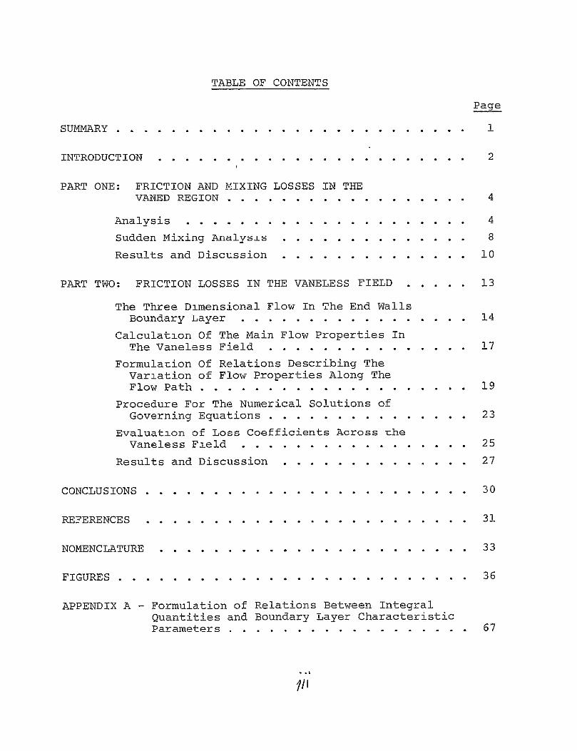
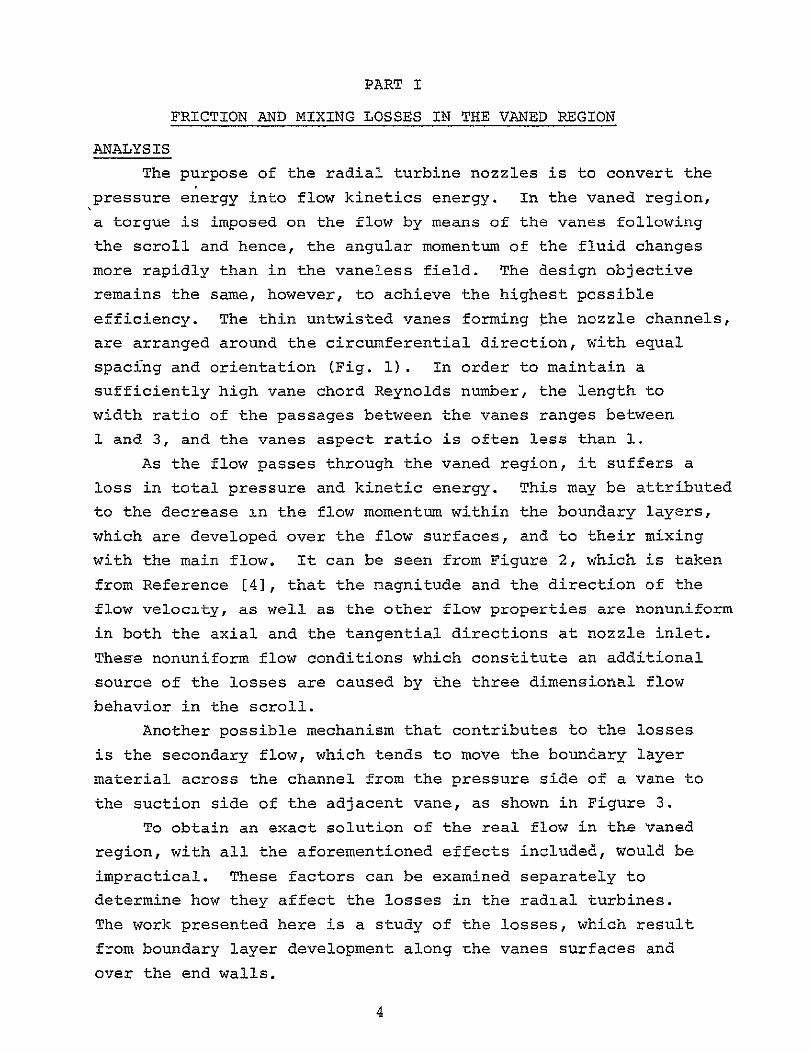
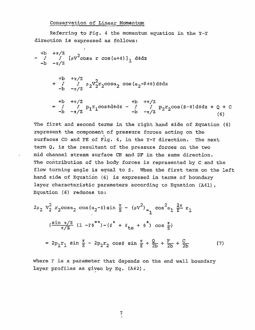
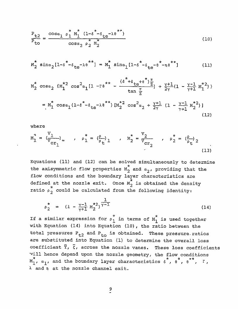
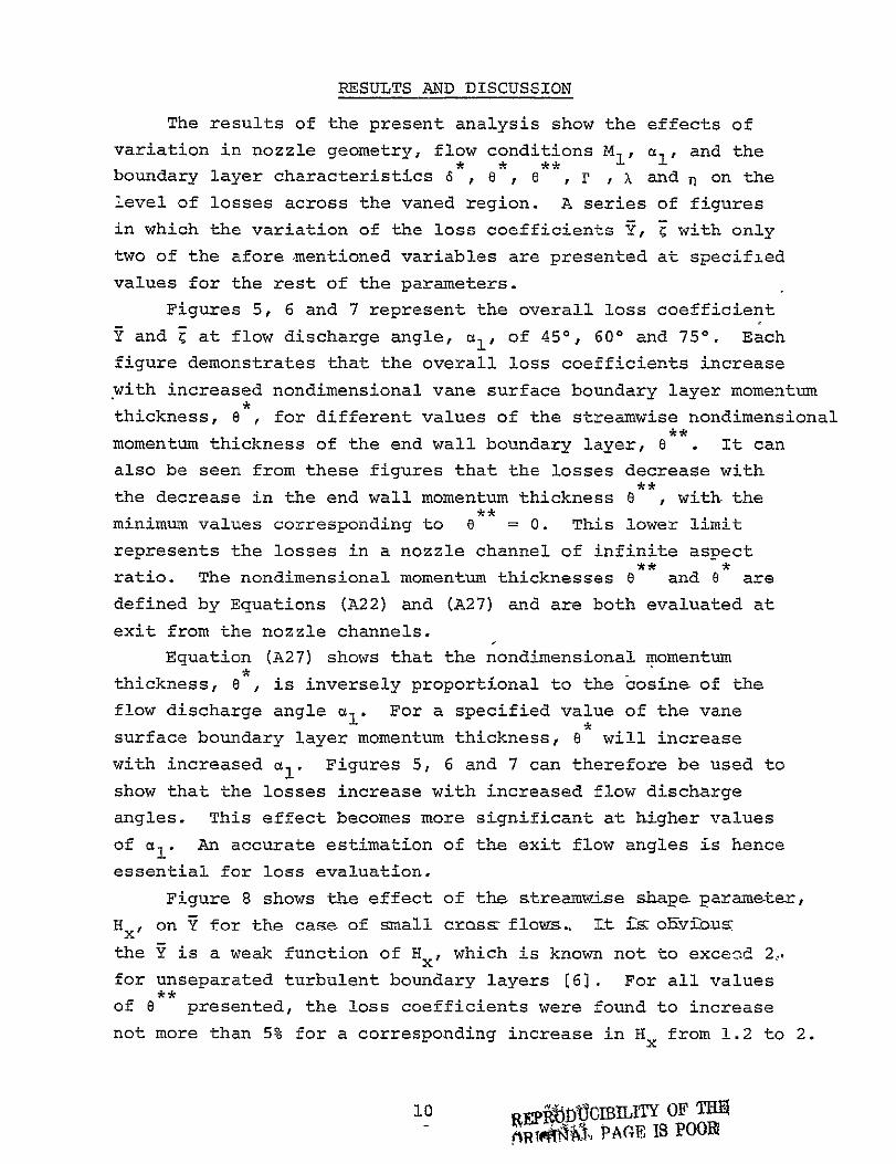
RESULTS AND DISCUSSION
The results of the present analysis show the effects of
variation in nozzle geometry flow conditions M1 a and the
boundary layer characteristics 6 8 r X and n on the
level of losses across the vaned region A series of figures
in which the variation of the loss coefficients Y with only
two of the afore mentioned variables are presented at specified
values for the rest of the parameters
Figures 5 6 and 7 represent the overall loss coefficient
and E at flow discharge angle a1 of 450 600 and 750 Each
figure demonstrates that the overall loss coefficients increase
with increased nondimensional vane surface boundary layer momentum
thickness a for different values of the streamwise nondimensional
momentum thickness of the end wall boundary layer 8 It can
also be seen from these figures that the losses decrease with
the decrease in the end wall momentum thickness 8 with the
minimum values corresponding to 8 = 0 This lower limit
represents the losses in a nozzle channel of infinite aspect
ratio The nondimensional momentum thicknesses 8 and 0 are
defined by Equations (A22) and (A27) and are both evaluated at
exit from the nozzle channels
Equation (A27) shows that the nondimensional momentum
thickness 8 is inversely proportional to the cosine of the
flow discharge angle aI For a specified value of the vane
surface boundary layer momentum thickness a will increase
with increased aI Figures 5 6 and 7 can therefore be used to
show that the losses increase with increased flow discharge
angles This effect becomes more significant at higher values
of a1 An accurate estimation of the exit flow angles is hence
essential for loss evaluation
Figure 8 shows the effect of the streamwise shape parameter
Hx on Y for the case of small crQss flowas t s olvibun
the Y is a weak function of Hx which is known not to exceod 2
for unseparated turbulent boundary layers [62 For all values
of a presented the loss coefficients were found to increase
not more than 5 for a corresponding increase in Hx from 12 to 2
10 -bpftDIBIL1TY OF THF
~ 1RTMM PAGE IS POOR-
Since the vane trailing edge thickness te is increased
when cooling of the radial turbine is considered it would be
desirable to examine the effect of te on the overall losses
in some detail This effect is investigated through the use
of the parameter t + + p- The results are presentede s pr21
in Figure 9 as the ratio between the loss coefficient Y at
a finite value of t to Y calculated for zero trailing edgee thickness Figure 9 shows that the increase in the losses can
be considerable for larger values of the trailing edge thickness
Under normal operating conditions corresponding to 6 = 002
and e = 0015 in a conventional turbine with trailing edge thickness parameter t +6 +6plvz of about 003 the
e s r trailing edge contributi6n to the losses is about 25 percent
If the parameter t +S +6 2 Z is increased to 007 thee s p r1
portion of the losses due to the finite trailing edge is
increased to 82 percent
The effect of compressibility on the overall loss coefshy
ficients are shown in Figures 10 and 11 It can be seen
from Figure 10 that the enthalpy loss coefficient remains
practically constant with increased free stream Mach number
for the different values of the boundary layer parameters
considered On the-other hand the overall total pressure
loss coefficient Y increases significantly with increased
Mach number Figure 11 Due to the large sensitivity of the
pressure loss coefficient to Mach number variations it is
recommended to use the overall enghalpy loss coefficient C
in describing the loss performance characteristics of the
radial turbine nozzles
The effects of the end wall boundary layer cross flamp on
the losses are shown in Figures 12 and 13 Figure- 12 illutrate
the variation of Y with 0 for the different end wall
velocity profiles A B C and D of Table A-i in Appendix A
Since it was found previously that the loss coefficients
are weak functions of Hx it may be concluded by examining
Figure 12 that the cross flow profile parameters K and L
(see Equation A9 and A10) have a significant effect on the
losses As an example for a value of the nondimensional
1
streamwise momentum thickness 8 of 003 a variation in the
magnitude of losses up to 25 can result by considering
different profiles
Figure 13 shows the contribution of the cross flow to
the losses which were calculated using the end wall velocity
profile B It is clear from the figure that the minimum
losses are obtained for the case of collateral end wall boundary
layers e = 0 The losses increase appreciably for strong
cross flow cases corresponding to higher values of s
12
PART II
FRICTION LOSSES IN THE VANELESS FIELD
The vaneless nozzle in a radial turbi-ne consists of a smooth
walled axisymmetric passage with radial or conical surfaces The
passage depth may change with radius but a little influence on
both the pressure and velocity distribution is noticed since the
angular component of the fluid momentum is predominant Basically
the flow in the vaneless nozzle can be treated as a vortex motion
except for the skin friction which acts upon the flow boundaries
In overcoming the resistance along its path the flow loses part of
its total pressure The pressure loss occurs at the expense of
both static and dynamic pressure (8]
Loss analysis for the turbine vaneless nozzle may be treated
using the same methods developed for the compressor vaneless
diffuser provided that the area changes as well as the flow
direction are taken into consideration Conventional flow
analyses for the vaneless diffuser [9 10 11] were based on the
assumption of one dimensional flow Total pressure losses were
determined using a constant friction coefficient In a recent
study Jansen [12] arrived at a more accurate evaluation for the
friction coefficient and its variation along the flow path
His analysis however requires much more detailed knowledge of
the flow conditions than can actually be realized in practice
In the following study the governing equations for the flow
in the vaneless space are formulated using three dimensional end
wall boundary layer theory [6] The resulting differential equations
are solved numerically to obtain the flow properties within the
vaneless field The losses are evaluated taking into account both
the wall friction and the momentum flux changes due to velocityshy
profile variation along the flow path The effects of some
parameters representing the operating conditions and nozzle
geometry on the losses incurred within the vaneless field are
also investigated
13
THE THREE DIMENSIONAL FLOW IN THE END WALLS BOUNDARY LAYER
Flow Pattern
As the flow in the vaneless field proceeds towards theimpeller tip the main streamlines turn as shown in Fig 14
A balance is established in the main stream between the static
pressure gradients and the centrifugal forces caused by the flow
turning The unbalance between the externally imposed pressure
gradients and the centrifugal forces of low momentum end wallboundary layers produces an acceleration component normal to
the main stream direction in the boundary layer fluid
Consequently the velocity in end wall boundary layers is
different from the mainstream velocity V not only in magnitude
but also in direction The velocity profiles in this skewed
boundary layer is shown in Fig 15 Taylor [13) noticed that
the polar plot of the velocity vector in a skewed boundary layer
follows a triangular form such as shown in Fig 15 Thus
any analysis of such boundary layer is usually carried out using
different formulation in the inner and outer sublayers
The Inner Sublayer
Referring to Fig 15 the following linear relation between
the cross flow velocity component w and the streamwise velocity
component v holds good
w = v tan tmax (15)
The angle pmax in the last equation is invariant within the
collateral inner sublayer Accordingly it can be estimated
at the wall using the following relation
tan max Limit S (16)-- =
Since the skin friction is in the same direction as the velocity
vector at the wall therefore it will deviate by the angle
max from the main flow direction If the wall shear stress
and the friction coefficient are denoted by Tr0 and Cf respectively
14
and if their components in the main flow direction by -cx and
Cfx then
Cf = Cfx(l + C2 )12 (17)
where
T
Cf 1 2 (18)
and
T 2C = 1V (19)
Ludwieg and Tillman [14] deduced an accurate semi-empirical
expression for the wall friction of two dimensional flows in
the presence of favorable pressure gradients Johnston [61
showed that in a skewed boundary layer the relation of
Ref [141 can be used to determine the component of the skin
friction coefficient in the main flow direction according to
the following relation
-0268 Cfx = 0246[ExpC-l561 Atx)JRe (20)
where Hx is the streamwise shape factor and ROx is the
Reynolds number based on the streamwise momentum thickness
Referring to Fig 16 the components of shear stresses in
the tangential and the radial directions are
x6 = T0 sin( t-max) (21)
t= T0 max)a (22)Tr o cos(a -
When Equations (16) (17) and (18) are substituted in Equations
(21) and (22) the following relations are obtained
e 1 PV2Cf[Sin - pound cosc] (23)
15
1 pv2CfxECOS + e sina] (24)
In the above equations the values of a and s will depend
on the main flow variables The expressions which are used in
evaluating these parameters are given in the outer sublayer
analysis that follows
The Outer Sublayer
The two velocity components in the non-collateral cuter
sublayer namely the cross flow component w and the streamwise
component v are related by the following equation
w = A(V - v) (25)
The parameter A depends on the main flow turning angle (0)
which is shown in Fig 14 and is given by the followin expression
A =-2V 2 dS (25a)0 V
where V is the main flow velocity
The tangent s of the limiting angle m can be expressed
in terms of the parameter A and the streamwise friction coefficient
Cfx according to the analysis of Ref 16] as
+)14
- 01 + - 1 (25b)
fx
Equations (20) (25) and (25b) can be substituted into Equations
(23) and (24) to predict the variation of shear components t Tr
along the flow path in terms of main flow variables The details
of the computation procedure used for this prediction is
presented in the section dealing with the Numerical Solution of
the Governing Equations
16
CALCULATION OF THE MAIN FLOW PROPERTIES IN THE VANELESS FIELD
Analysis
The vaneless space geometry together with the velocity
triangles and the coordinate system are shown in Fig 17 It is
assumed that the flow enters the vaneless field at the radius
r2 in a steady uniform axisymmetric pattern with specified
flow conditions These inlet flow properties are determined
from the vanes friction and mixing loss analysis presented in
Part I of this study
As the flow passes through the vaneless field there will
be a variation in its properties in both radial and axial
directions The variation in the axial direction z results
from the development of boundary layer over the two end walls
The static pressure distribution and the radial and tangential
velocity components will be determined along the main flow path
using the assumptions of the first order boundary layer theory
An equivalent one dimensional flow will be considered in a
nozzle with an effective depth of 2be t which is equal to the
actual nozzle depth 2b minus the displacement thicknesses
of the two end wall boundary layers at any radius r (see
Fig 18) The components of the velocity V and the pressure
p of the flow passing through this equivalent nozzle vary
only along the radial direction and are independent of z and
e The total pressure loss due to friction will be calculated
using the values of Tr and T developed in the previous section
and given by Equations (23) and (24)
Equations of Motion
The control volume of Fig 19 will be used in the following
derivation The magnitude of the velocity V is considered to
increase as the flow proceeds inward in the vaneless nozzle
Furthermore the flow will be assumed to be steady and adiabatic
17
Conservation of Angular Momentum
Setting the net efflux of angular momentum through the
control volume equal to the external torque due to the shear
force in the tangential direction we obtain the following
relation
PbeV cosa (r V sina) = Ter (26)
Substituting for T from Equation (23) into Equation
(24) we get V cos__Vsin_ d CfXV2
Cosa V sina + V cosa - (V sina) = r[sina - scosal r dr 2be
(26a)
Conservation of Linear Momentum in Radial Direction
d PbeV2sin 2 a-PbeV Cosa -( CVcosa) = bedr (P)- 27)
The left hand side of the above equation is equal to the net
radial momentum flux The first two terms on the right hand
side are the radial components of the pressure forces and the
wall friction forces while the third term represents the
centrifugal forces
Substituting for Tr from Equation (24) into (27) and
rearranging we obtain
dp Cfx 2[s nsin2a 2d oe p dr 2be r-Vcsdr V r-V coscoa - _ V [Cosai + esinalshy
(27a)
Conservation of Mass
From continuity considerations the following differential
equation is obtained
18
I dp + 1 d(V cos) +1 1+ dbe
pdr V cos dr r bdrshye
Equation of State
The pressure density temperature relation for a perfect
gas is used in the following differential form
l dp 1 dp 1 dT (29)p dr p dr T Ur
Energy Equation
Since the total temperature remains constant during the
expansion process in the vaneless field the differential form
of the energy equation may be written as
M2d-y-l 2
1 dT _ M 1 dM2 (30) M2T dr 1 + yl 2 dr
M2 Which when combined with the definition of the Mach number
reduces to
1 dV2 1 2 1 d v 1- I I (30a)
M IdrY-l2V2 dr 2
Formulation of Relations Describing the Variation of Flow Properties Along the Flow Path
Equations (26) through (30) will be manipulated to obtain
the following relations which are used to calculate the pressure
Mach Number and the main flow angle
Pressure Distribution
Combining Equations (29) and (30a) the following relation
is obtainedp-i M2 2
1 dp 2 1 dMdp p dr p d-r 1+ X31M 2 d
2 M
Dividing Equation (27a) by V2cos2a and using the identity
pV2 = yp M2 (32)
gpRUCIBL1TY OF THE19 z POOR16gVOAL PLO
one gets an expression describing the variation of the tangential
velocity component with radius as
1 d 1 1 dp Cfx (cosa + ssin) tan2 a Cosa dr (V cosa) 2o2P - - 2e 2 ryMCos a e Cos as
(33)
Substituting for 1 do from Equation (31) C1osa r (V cosa)p dr
from Equation (33) into the continuity Equation (28) the
variation of pressure with radius is deduced as
1 dp M2 Cfx (cosa + Esina) sec2a p dr 2 2 [- 2 r
M -sec eO aoc
y- M2 2 db - 1 M 1 dM 1 e (34)
-1 2d2r Fbdr-
Mach Number Distribution
In order to obtain the variation of Mach number along the
flow path an additional equation relating the pressure in terms
of M and a is required This relation is obtained by combining
the equation of angular momentum (26a) with the equation of
linear momentum (27a)
1 1 dp Cfx 1 1 dV2 (35)22p dr 2b Cosa)c 2 v dr
Substituting Equations (30a) and (32) into the last equation
it reduces to
1 dp = yM2 -1 1 d2 Cfx (36)) M2 dr + 5ecoSaN-+ 12pd-r--2
Now eliminating dp between Equations (34) and (36) the
p dr
Mach number variation along the radius r is obtained from the
resultant expression
20
1 dM 1 ( 2 2 fx 2 be21M 1sect + C sec(M - tan2 a + Etana)+ e
M2 2 r 2beg d
(37)
Flow Direction
The differential equation of flow direction may be developed
using the following relation
tana = V sin (38)
V cosa
This last equation can be written in the following differential
form
I d(tana) _ 1 d(V sina) 1 d(V cosa) tan dr s dr V cosat r (38a)
Substituting Eq (26a) and (33) intoEquation (38a) the following
relation is obtained
2 21 d(tana) _ sec a 1 dp sec (39)
tana dr yW-2 p dr r
1
Substituting for from Equation (34) and rearranging the
equation describing the variation of flow direction with radius
takes the following form
M2d- -tana Cfx sec [ 2 an++ db er b [i +Cy-l)M stan+2dr M sec a e e -d shy
(40)
Nondimensional Form of the Governing Equations
Before solving the equations of motion they will first be
written in a nondimensional form The nozzle dimensions will be
normalized with respect to the inlet radius r2 and the pressures
with respect to the total inlet pressure Pt2 as follows
2bR -rep r B e P 2 F2 Pt2
271
Equations (34) (37) and (40) can therefore be written in
the following nondimensional form using the above expressions
yM2 2I dP _ s Cfx (cosa + Esin) sec aP dy 2 s e 2 B 2 r
(~ 1 2 1d(421+ Y- M 2 ) M-I Y- - N I
2
1 dM 1 +Y M2 [sec2 a Cfx 2_ 2 d-R M2 _ seci (yM2tana3Ba T-
M _ sec aciB-
(43)
and
M2dM -tan Cf seca 2 lYB
2 dR M2_ sec2aRBd (1 +(yl)M+ etan)+ -- (44)
Furthermore if the thicknesses of the boundary layers developed
over the two end walls are taken to be equal then B the depth
ratio and its derivative could be expressed as
B 2b 26 (-) ( 5 =--- - -2d r r2 dR dR
where S is the streamwise displacement thicknessx
22
PROCEDURE FOR THE NUMERICAL SOLUTION OF THE GOVERNING EQUATIONS
In order to determine the flow properties within the vaneless
field the system of nonlinear differential Equations (43) (44)
and the algebraic Equations (20) (Z5a) and (25b) will be solved
A fourth order Runge-Kutta algorithm is used to solve the
simultaneous first order differential Equations (43) and (44)
The solution procedure consists of the following steps
1 The values of M a at the vaneless nozzle inlet are
assumed to be known from the analysis given in Part IdB
2 At any radius Ri f knowing Mi ai Cfx e B and -B
the increments in M and a over the radial distance (-AR) is
computed using the following recursion formula
N -M= _AR (K + 2K + 2K + K (46)i+1 -46 C= 2 23 + + +ai+l -ai = - A-R (KK 2KK 2KK KK (47)
1 1(12 213 1(4)
where
K= f(Ri M i ai)
KK 1 = g(Ri M i ai )
1AR K K
K2 i + --- ) (48)
KK 2 = g(R i AR M + K1 KK1
2- - L +-)
K3 f(Ri AR M 2 a+K21 2 i 2 i 2
KK 3 g(Ri AR +K2 KK23 2 i 2 i
23
K(4 f(R - AR Mi +K i + KK 3 )
KK4 = g(R i - AR M + K3 ai + KK 3 )
Where f represents and g d and are evaluated according dR U-R
to Equations C431 and C441 respectively using the known values ofCfx A e B and q- at the radius Ri
C f x ld R
3 At the end of the interval at the new-radial location
Ri - AR the quantities Cfx A E B and dB are evaluated using
Equations (20) (72ay and (25B respectively as will be explained
The streamwise friction coefficient Cfx is calculated according to
Equation (20) The boundary layer characteristic parameters ROx and
Hx in this equation can be evaluated using any method of
boundary layer solution In the present analysis the method of
Reference 15 was used for this purpose Integrating Equation (25b)
numerically starting from the vanalea nozzle fl-let until anshy
desired radius where the mean flow turning angle $ is known
gives the corresponding value of A at Ri1 These values of Cfx
and A are then substituted into Equation (25c) which is solved
for e using an iterative procedure
4 Refined values for Mi+ci+l at (Ri - ARI are obtained1
by substituting the arithmetic average between Ri and Ri+1 of the
variables Cf e B and - in the recursion formula (46) and (47)dR
5 The corresponding values for Cfx A e B - at R
are calculated as shown in Step 3 using the values of Mi+I
li+l obtained from Step 4
6 Steps 4 and 5 are repeated until successive values of the
computed flow variables are within the required accuracy in the
present study an accuracy of 0001 was maintained in the different
variables which was achieved after 2 iterations
7 The whole procedure (Steps 2 through 6) is repeated for
small values of (-AR) starting from the nozzle inlet up to the
impeller tip The numerical results reported herein were
calculated using radial increments AR equal to 001
24
EVALUATION OF LOSS COEFFICIENTS ACROSS THE VANELESS FIELD
Standard definitions of total pressure and enthalpy loss
coefficients in terms of the average pressures at inlet to and
exit from the vaneless region are adopted The total pressure
loss coefficient is given by
P t3
- t2 (49)
P 3
Pt2
while the enthalpy loss coefficient may be written as
Y-1Pt2 P t3t3 (50)(Pt2 -shy
P3
It is clear from the above two equations that the flow conditions
at station 3 the vaneless space exit have to be known in order to
calculate the loss coefficients
In the previous chapter it is explained how to determine
numerically the Mach number the flow angle and the effective
nozzle depth variations along the flow path Knowing the values
of these variables at the nozzle exit (-station 3) the static and
total pressures P3 and Pt3 are computed using the equations
derived below
The conservation of mass between the vaneless diffuser inlet
and exit is expressed as
P2V2cosa 2r2b2 = P3V3cosa 3r3be3 (51)
where 2b is the effective depth of the nozzle at station3
If the definition of Mach number and the equation of state
are substituted into the above Equation (51) the following
expression for p3P2 is obtained
25
P b2 r2 Cosa2 M2 I + 1-__ M2p3 2 2_ c 2 2
(52)2 bre r3 cosa3 M3 1 + yiM2
3 2 31
The total pressure at the vaneless space exit Pt3 is then
determined using the following relation
Pt3 P3 1 2 3 T-Pt2 =P 1 + y-- M2 (53)Pt2 P22 2
Equations (52) and (53) are sufficient to determine the loss
coefficients Y and provided that the inlet flow conditions to
the vaneless space are specified
26
RESULTS AND DISCUSSION
The numerical examples worked out using the present method of
analysis are presented in two groups In the first group the
effects of inlet flow conditions on the flow behavior and losses
in the vaneless field are investigated The second set of
results illustrate the influence of changing the end wall spacing
on the same flow parameters
1 Effects of Inlet Flow Conditions
The effect of two inlet flow parameters namely the Mach number
and the flow angle on the vaneless nozzle performance are considered
first Computations were carried out with an inlet Mach number of
08 and different inlet flow angles a2 the corresponding results
are shown in Figures 20 to Z2 On the other hand the data obtained
with different Mach numbers for a constant inlet flow angle of 70
are presented in Figures 23 to 25 The geometrical end wall spacing
2b and the inlet radius to the vaneless field r2 for this first
set of results were chosen to be 0339 and 393 inches respectively
The total temperature was held constant throughout the flow at 20000R
The change in angular momentum ratio r3V3sin 3r2V2sina2
with the normalized radius R is shown in Figure20 for different
values of inlet flow angles a2 It can be seen that
increasing a2 causes a reduction in the angular momentum ratio
everywhere This effect becomes particularly predominant at
high values of inlet flow angles For example at a normalized
radius of 09 the angular momentum ratio changes from 0992 to
0987 corresponding to an increase in a2 from 600 to 700
Meanwhile a further increase in a2 from 700 to 800 results in
a reduction of the same parameter from 0987 to 09732 2The radial variations of the ratio M3M2 are shown in
Figure 21 for three different values of inlet flow angle It can
be seen from the figure that increasing a2 reduces M3M 2 at each
radius This is a consequence of the larger reduction in the
tangential velocity component due to viscosity an influence
that dominates the augmentation in the smaller radial velocity
component It can also be concluded that for all the values of a2thrti M2 2
the ratio 3M2 increases as the flow proceeds inwards Thich is
anticipated
27
The variation in the pressure loss coefficient Y and
enthalpy loss coefficient C are shown in Figures 22a and 22b
respectively It is clear that both coefficients increase with
increased inlet flow angle a2 at every radial location If
the results of Figure 22 are compared with those obtained in
Part 1 it can be concluded that even for the largest values of
a2 the loss coefficients in the vaneless field are extremely
low as compared to the losses in the vaned region For example
the pressure loss coefficient of Figure 22b is as low as 00125
at R = 090 for values of a2 and M2 of 600 and 08 respectively
On the other hand the pressure loss coefficient of Figure 8
is as high as 0107 under the same operating conditions
Briefly one can conclude that increasing the inlet flow
angle a2 results in a larger reduction in the total pressure
Mach number and angular momentum at nozzle exit This can be
attributed to the longer path that the flow has to take to reach
a certain radius if the inlet flow angle is increased
The effect of changing the inlet Mach number M2 on the
angular momentum ratio is illustrated in Figure 23 It is
evident that at any radius the drop in angular momentum due to
viscous losses is smaller for high values of M2 Accordingly
high Mach numbers at inlet to the turbine vaneless field are
recommended The variation in the ratio M2M2 is shown in
Figure 24 for different values of inlet Mach number It is
obvious that the acceleration rate in vaneless field is higher
for larger inlet Mach number
The pressure and enthalpy loss coefficients Y and c are
shown in Figures 25a and 25b respectively It is clear that
the pressure loss penalty paid due to viscous effects at any
radius ratio is not strongly affected by the inlet Mach number
Furthermore the enthalpy loss coefficient at any radius remains
practically constant for all the inlet Mach numbers investigated
2 Effects of Nozzle and End Wall Spacing
The object of the second group of numerical examples is to
study the effect of the geometrical passage depth 2b on some flow
28
properties and on the loss characteristics in the vaneless
field For this purpose the following values of the passage
depth were considered 0262 0393 and 0785 with an
inlet radius to the vaneless field of 393 The corresponding
values of the nondimensional parameter (r22b) thus ranges
between 15 and 5 The results were obtained at 08 inlet
Mach number and 700 inlet flow angle with an inlet total
temperature of 2000R
Figure 26 represents the radial variations of angular
momentum ratio r3V3 sinc3r2V2sina2 for the three values
of the parameter (r22b) Although the angular momentum
ratio decreases at any radius Rywith the decrease in end
wall spacing 2b the curves indicate that there is only minor
differences between smallest and largest values of the2 2
parameter (r22b) The change in the ratio M3M2 with R
is shown in Figure 27 Increasing the passage depth 2b2 2
results in an increase in M3M2 at any radius ratio R22The increase in M3M2 results primarily from the reduction
in the friction surface area compared to the total flow area
as the wall spacing is increased Figure 27 also indicates
that the variation of nozzle end wall spacing 2b has a
small influence on the Mach number distribution within the
vaneless space
The influence of the end wall spacing on flow losses is
shown in Figures 28a and 28b It is clear that larger losses
are incurred as the nozzle passage becomes narrower corresponding
to high values of r22b It is important to emphasize once
more that even for the large values of (r22b) the losses
in the vaneless field remain relatively low as compared to
the vaned region losses
29
CONCLUSIONS
An analytical model which is based on the observations
obtained from an experimental study was developed to predict the
losses in a radial nozzle annulus The contributions of the
end wall boundary layers to the losses was found to be several
times that of the vane surface boundary layers This influence
is particularly significant when the end wall boundary layers
are characterized by large cross flow components Under the
stipulation of the analytical model in which the mixing losses
are lumped with the friction losses in the vaned region a small
portion of the overall losses were contributed by the viscous
effect in the vaneless field Experimental findings in which
stator-rotor interaction effects are not considered show that
the losses are influenced by flow nonuniformities at inlet to
the nozzle channel and by secondary flow These factors need
further investigation if a realistic estimate for the losses
is to be obtained analytically
It is concluded that generally the losses in a radial
nozzle assembly would not be greatly affected by the addition of
a large vaneless space Also if the nonuniformities of the
flow discharged from the vaned region can be reduced the
efficiency of the assembly as a whole would be improved Thus
the loss penalty paid during an expansion process resulting in
the required flow properties at rotor tip from a specified
outlet flow condition from the scroll could be minimized
Such minimization is achieved by a proper selection of vanes
configurations in conjunction with a suitable vaneless space
dimension The application of the compositive method of analysis
presented allows one to differentiate between various suggested
radial nozzle designs in order to select the optimum configuration
30
REFERENCES
1 Todd Caroll A and Futral Jr Samuel M A FORTRAN IV
Program to Estimate the Off-Design Performance of Radial
Inflow Turbines NASA TND-5059 1969
2 Futral Jr Samuel M and Wasserbauer CA Off-Design
Performance Prediction with Experimental Verification for a
Radial-Inflow Turbine NASA TND-2621 1965
3 Baljie OE A Contribution to the Problem of Designing
Radial Turbomachines Trans ASME Vol 74 1952 pp 451-472
4 Tabakoff W and Khalil I Experimental Study on Radial
Inflow Turbine with Special Reference to Loss Prediction
University of Cincinnati Department of Aerospace Engineering
Report No 75-50
5 Stewart WL Analysis of Two-Dimensional Compressible-Flow
Loss Characteristics Downstream of Turbomachine Blade Row
in Terms of Basic Boundary-Layer Characteristics NACA
TN 3515 1955
6 Johnston JP On the Three Dimensional Turbulent Boundary
Layer Generated by Secondary Flow Trans ASME Journal of
Basic Engineering Series D March 1960 pp 233-247
7 Dring RP A Momentum Integral Analysis of the Three-
Dimensional Turbine End-Wall Boundary Layer ASME
Paper No 71-GT-6
8 Vavra M Aero-Thermodynamics and Flow in Turbomachines
John Wiley New York 1960
9 Polikovsky V and Nevelson M The Performance of a Vaneless
Diffuser Fan NACA TM 1038 1942 (Trans of Report 224 of the
Central Aero-Hydrodynamics Institute Moscow 1935)
10 Brown WB and Bradshaw GR Method of Designing Vaneless
Diffusers and Experimental Investigation of Certain Undetermined
Parameters NACA TN 1426 1947
11 Stanitz John D One-Dimensional Compressible Flow in Vaneless
Diffusers of Radial and Mixed-Flow Centrifugal Compressors
NACA TN 2610 January 1952
31
12 Jansen W Steady Flow in a Radial Vaneless Diffuser
Journal of Basic Engineering Transactions of ASME Series
D Vol 86 1964 pp 607-619
13 Mager A Generalization of Boundary Layer Momentum
Integral Equations to Three Dimensional Flow Including
Those of Rotating Systems NACA Report 1067 1952
14 Ludwieg H and Tillmann W Investigation of the Wall
Shearing Stress in Turbulent Boundary Layers NACA TM 1285
May 1950
15 Truckenbrodt E A Method of Quadrature for Calculation
of the Laminar and Turbulent Boundary Layer in Case ofPlate and Rotationally Symmetrical Flow NACA TM 1379
May 1955
32
NOMENCLATURE
Symbol
A parameter (see Eq 25b)
B depth ratio defined as 2ber2
2b axial depth of the nozzle - distance between the
two end walls ft
2be effective depth of the nozzle
Cf skin friction coefficient
G streamwise profile function
g cross-flow profile function (see Eq A7)
H streamwise shape factor for the end walls boundary
layers (see Eq A8)
KL profile parameter for the end walls boundary
layer (see Eq A9 A10)
M Mach number dimensionless
M critical Mach number dimensionless
n coordinate normal to the vane surface ft
P pressure ratio defined as PPt2
p static pressure lbfft2
Pt total pressure lbfft2
r radial coordinate ft
R radius ratio defined as rr2
Rex Reynolds number based on momentum thickness of
the main flow dimensionless
T temperature OR
te vane trailing edge thickness ft
v streamwise velocity component in the boundary
layer over the end walls ftsec
33
V velocity ftsec
w cross-flow velocity component in the boundary
layerover the end walls ftsec
Y overall total pressure loss coefficient
z axial coordinate ft
Z number of vanes dimensionless
a angle between flow direction and inward radial
direction radians
8 main flow turning angle radians (see Fig 14)
y ratio of specific heats dimensionless
r parameter (see Eq 6A)
a boundary layer displacement thickness ft
ate trailing edge blocking factor defined as
te w rlcosal )
a total nondimensional displacement thickness over the
vane surfaces defined as (S +8 )(2-w r Cosa
a streamwise total nondimensional displacement thickness
over the two end walls defined as (ux + zx)2b
e boundary layer momentum thickness ft or angular
coordinate in plane normal to axis of rotation radians
a total nondimensional momentum thickness over the vane
surfaces defined as (6 +e )(- rlcos a) s p Z 1
e streamwise total nondimensional momentum thickness
over the two end walls defined as (eux+ezx)2b
X parameter (see Eq A23)
density lbft3
p
n parameter (see Eq A31)
w angle of limiting wall streamline and T with
respect to Vfs
34
T 0shear stress at the wall
overall enthalpy loss coefficient
etangent of the limiting streamline defined as tanw
Subscripts
0 inlet to radial nozzle outlet from the scroll
1 nozzle exit
2 station at which uniform conditions are assumed to
take place
3 inlet to rotor
c cross flow direction
cr critical conditions
local conditions outside the boundary layer regions
9 end wall iower surface
p vane pressure surface
s vane suction surface
t total conditions
u end wall upper surface
r radial direction
x streamwise direction
35
STAT IONMID-CHANNEL STREAMLINE
SUCTION SURFACE
PRESSURE SURFCEI -
VANELESS SPACE rNOZZLE -0
CANLIMPELLER TIPI l0
-NOZZLE
THROAT
RAPID ADJUSTMENT FIG 1LOW RE N-S AN VTG Z
FIG1 FLOW REGIONS AND VELOCITY DIAGRAMS FIG 8
II
SUCTION SIDE PRESSURE SIDE IPr= 105 meter Hg Z -LEADING EDGE
S0 o 3 0 1o 20 3o 410
PERCENT OF SPACING
030------ shy
- 0 0--- 0shy
a - TOTAL PRESSURE = - Pto) I Pr PERCENT
010205
20195 0195
b- MACH NUMBER
6 67 68 69 70
65shy_____6
c- ANGLE do (DEGREE)
FIG2 FLOW PROPERTIES AT STATION 031
POSITION
50
Li205
SUCTION SIDE ail PRESSURE SIDE
Pr= 105 meter Hg TRAILING EDGE POSITIOt
80 60 40 20 20 40 60 80 ]I I p
PERCENT OF SPACING
-038
a - TOTAL PRESSURE = ( PtP2)P r PERCENT
b - MACH NUMBER
76 79 777
76 75 74 shy
s2 _
c -ANGLE c2 (DEGREE) RfPROJJUCIBIL OF THE2 -afRkANampAGR 1BPOOR
FIG 3 FLOW PROPERTIES AT STATION 1
38
STATION 2-- NOZZLE VANE
F
MIDOHANNEL STREAM SURFACE
DEVELOPED VIEW
F-E
(kA -ION ST T
MIOCHANNEL STREAM SURFACE (Ct
FDEVELOPED-VIE
YA
RIG 4 CONTROL VOLUME
39
- ANGULAR SPACING =277 0 p 020-
V) ( te8s+8p ) 003w o -- - - -05Z 2wv
z
c- deg002- 016- =45 003
014
01000shy
lt GOB (9
I-shyz [i 006
0
It 0040 U
02
0 001 002 003 Q04 NONDIMENSIONAL MOMENTUM FHICKNESS 0
FIG 5 LOSS COEFFICIENTS
40
Igtt
14p 020 ANGULAR SPACING 277003
z 018 Le+s+op z 04 cc 6O 002
Nw 016 Hx 2
N 00 E =00 001z 0-14-
Ji M=08 _02
001lt 00
o 010
0 0 lt 000Cl)
lt 004
0 u
Y0 V002
-0 001 aO2 0-03 004
0NONDIMENSIONAL MMNU THICK NESS
FIG 6 LOSS COEFFICIENTS
4z Djw4Lm PAt is POOR
W ANGULAR SPACING 277 Z2
Li-(teI+s+Sp)- r =005
-J030-N 0
Z HX20 003 025 =-00
-- 0002
= 08 003020o M 1 _ooi 0 -00 2
i 020 -00 M E M HS
z420 -
U 015 0ltr1 0031 0
u-IshyFI7 OSCOFICET
0 42
0-20shy 0 0
ANGULAR SPACING = 277 r--shy
0-18 ( tedeg3sa P ) O005 0-03
016 z 002
cri = 60
Igt- 0-14 E =00 001
012 M =05
Wi 000 9 010shyLL
i
[Hx = 10 004W~ jur 2ILfU)0 002shy_jHG S EFETOFH PAAEE H)O
00 00 0=0 0230-4 000 001 02 003 004 00
0043 u43
30
001
0020
a =60 003 28
H =20x =00
o 001(J
24 002-002 CCV
Igt- 003I) Jshy
C) 001
-20 02 003
00
y
16 0 t7t-
12
100 002 0-04 006 O08 010
(t + 2+7T1f e s p
FIG9 - EFFECT OF TRAILING EDGE THICKNESS
44
C
ANGULAR( te+CSs+3pD
018 )
SPACING
= 005
=277
c = 600 o18shy -zshy q
0416 0 004003
014shy0-030030-04 0-02
012shy 02 0-03 -0-03 002 -004001
w 001 003 5 010 002 0-02 L 003001
0 OB
001 002 002 1001
ul 006 0
5j 001 5001
004
a Hx 20 - 002-
I 0
0 02o 04 05 06 07 08 09 MACH NO
PIG1O VARIATION OF ENTHALPY LOSS
COEFFICIENT WITH MACH NO
45
04 amp03 022-
ANGULAR SPACING 277
020 (te+ s -) = 05 03amp03
r01 2 -IT0
04amp02
0-18shy a=60
-02 amp30
016shy 04 amp -01
0-14shy -1~ amp 03
Z X -02 amp 02 IL 03 amp -01 C) 012
u 00 amp -03
01 amp 02
0
0-0-Lo
amp01
bi
W 00shy 0020 amp00 -_ H00 amp20
I I I I0 02 04 06 0-8 1
MACH NO
FIG11 VARIATION OF PRESSURE LOSS
COEFFICIENT WITH MACH NO
46
Igt-
ANGULAR SPACING = 277 nw (t + +8 ) K e s p 0-O02
zshyui 0
-J cz=6 0
o Si z 0003 lt 025 - E 0=O3
020shy
0 00
I--deg
PROFILE LUi 010 - A
B 0 005-shy CU
D ()
0 0 001 002 003 004 005
NONDiMENSIONAL MOMENTUM THICKNESS e
FIG -12 EFFECT OF END WALLS PROFILE
PARAMETERS ON LOSS COEFFICIENT
47
ii
ANGULAR SPACING = 277 u)zw (t + pXe s P-00
w2 03 00
N60 0p 0
Z2 _
W 0358z
Nia6
z 010 031 0 II1
00 5-1
003 X
O0 K = 243 0L
K1 = 0966OW 00 3 00 =043
- 0NONDMEN SIONAL MOMENTUM THICKNESS 4-
FIG 13EFFECT OF END WALLS CROSS FLOW
PARAMETER (E)- ON LOSS COEFFICIENT
48
0
REFERENCE DIRECTION
VANELESS SPACE INLET
MAIN FLOW STREAMLINE
- - ROTOR TIP
-BOUNDARY LAYER STREAMLINE
FIG14FLOW PATH IN THE VANELESS FIELD
CROSS BL MAIN BL INNER OUTER zSUBLAYER SUBLAYER
-V - 1 --shy 2
V V V w
SxTx Tangent to maiflow str line 1
VV
a VELOCITY PROFILES b-VELOCTY POLAR PLOT
FIG 15 END WALL BOUNDARY LAYER
TANGENT TO MAIN FLOW STREAMLINE
SV sina TANGENTIAL DIRECTION
ul
F d
0 Co VELOCITY VECTOR u AT THE WALL
rY w
J
0
FIG 16 VELOCITY AND WALL SHEAR STRESS COMPONENTS IN THE SKEWED BOUNDARY LAYER
station
aMain stream line
---- 2 -2Ii -----
U1 U
-- R otor tip
FIG 17 VANELESS SPACE GEOMETRY AND COORDINATE
SYSTEMshy
STAT ION 2b
7- Illlll shy
2b L2 be
Vel oc ity Geometry Geometry Velocity d istri but ion distribution
a - Actual case b - Equivalent case
FIG 18 ACTUAL AND EOUIVALENT VANELESS SPACE GEOMETRY
-------------
do Developed view
4 dPdr
dr
Vsinct NLbe 2
FIG 19 CONTROL VOLUME
A
Mz=08
10 C
d
O 099
0 0-98-
Z2 d7Q
0J0-97 -
097
085 090 095 10 RADIUS RATIO R
FIG 20 EFFECT OF INLET FLOW ANGLE
55
15 20
T cS14 -2214o
a= 60
lt
ryIti Ld In
Z
13
12 07-z
a= 70
02--80
110
085
FIG 21
090 095 RADIUS RATIO R
EFFECT OF INLET FLOW ANGLE
10
56
M2 08
Ishyz 005shy
0 0
LL0 IL
0tamp0 u 003shy
a 2 =70
a = 600
0 -U 002
U) U)
0L
001 -
0
05 090 095 10
LLI~ pRADIUS- RATIO R
FIG 22fa- EFFECT OF INLET FLOW ANGLE
0M05shy 0
z
i -
0
0 a06
LU 002-S0101
Il ampI I 00
085 0-90 0-95 10 RADIUS RATIO R
FIG 22 b EFFECT OF INLET FLOW ANGLE
deg a= 70
110
C 099shy
-M = 12ci
0
D
098shy
lt Mz= 05
0 8
H z w
0
097
2lt 096shy
(9 z
095 085
I 090
RADIUS
-
095 RATIO R
10
FIG 23 EFFECT OF INLET MACH NUMBER
1 7019
r4- M222 12
-17
0 Ishy
D z 13 r10 M =0f
11
1 095 10 RADIUS RATIO R
FI G 24 EFFECT OF INLET MACH NUMBER
60
LW
0
0
0024 - M -05
M42=0s
M=12
a=700 _
Ishy
z 0008 w
085 090 RADIUS
095 RATIO R
10
FI G25 a EFFECT -OFINLET MACH NUMBER
003 shy
-- M2 05 ashy0
0
Igtshyz ~ -shy v2 08
z w 002
LUc0
0
Lu
D
U)c)
085 090 095 10
RADIUS RATIO R
FIG 25b EFFECT OF INLET MACH NUMBER
013
- 099shyc~
r 2b
o 0-98 -
Cshy
r2 -15
H
z
090(2b
0
0-96shy
5
0-8096951
RADIUS RATIO R
FIG 26 EFFOT OF END WALL SPACING
63
15
M =08
a= 70
2 14
2b
O Ishy
r 13
2b
-10
z 2
12shy
10 085 090 095 10
RADIUS RATIO R
FIG 27 EFFECT OF END WALL SPACING
64
M2 =01
I--a2 70 z
w 2b
_0 002 2 b
w 0
5 090 09b5 10
~RADIUS RATIO
FI G 28 a EFFECT OF END WALL SPACING
M =OB a0
a2 = 70
w 0 =15
0U 003shy2b
Oi 002 2 b
LU[
001 - -
Lii
0 --shy
085 090 095 10 RADIUS RATIO R
FIG 28 bEFRECT OF END WALL SPACING
APPENDIX A
FORMULATION OF RELATIONS BETWEEN INTEGRAL QUANTITIES
AND BOUNDARY LAYER CHARACTERISTIC PARAMETERS
Al Basic Relations and Definitions
In this Appendix the integrals which appear in the left
hand side of Eqs (2) (4) and (6) will be determined in terms
of the boundary layer characteristics at station 1 To
accomplish this the domain of integral will be divided into
a main stream region and boundary region as shown in Figure Al
This is a generalization of the approach used in the two
dimensional analysis of Reference [5]
At exit from the nozzle channels the profile boundary
layer developed along the vane surfaces is collateral while
the end wall boundary layer is skewed The velocity vectors
within the skewed boundary layer can hence be resolved into a
streamwise component v and a cross flow component w The
displacement and momentuim thicknesses are used to describe the
boundary layers at station 1 These two quantities for the
collateral boundary layer are defined as
f pxr dn (Al)(pv
f f= pV dn-f- 2 dn (A2)
o (pV) o (pV)
Where n is the coordinate normal to the vane surface and 6f
is the boundary layer thickness On the other hand the streamwise
and cross flow end wall boundary layer displacement and the
momentum thickness are defined as follows
6f ax =f - f pV dz (A3)
0 (PV)7
67
V (A4)x f=f (PV dz - SfI (P2PV dz
af6 = dz (AS)
af 0 = f pw 2 dz (A6)
o (pV 2 )
Where z is the coordinate normal to the end wall surface
The relation between the parameters of equations (A3) through
(A6) can be determined for a given boundary layer profile
It is assumed that in the end wall boundary layer the streamwise
and the cross flow velocity profiles are given by Reference [63
v__ = Gw - sG g (A7) Vfs fs
In the above equations G and g are functions of the coordinate
perpendicular to the end wall z normalized with respect to the
boundary layer thickness (Sf) 6Eis the tangent of the angle
between the surface shear and the local main flow direction
as shown in Fig A2
The following streamwise and cross flow parameters are
used to describe the end wall boundary layers using the assumed
formes of the velocity profiles
f
x 0 (-pG)dzx o x x f(A8)
f (I-G)G dz 0
68
f 5 P(Gg)dz
cec f (A9)
I (v-iG)G dz0
6f 2
If p(Gg) dz
L e c ex f
(Al0)
I (p-pG) (G)dz 0
Where v is the nondimensional ratio pp
In Ref [7] various families of functions G and g that aremost compatible with the experimental data were determined
The corresponding profiles are plotted in Fig A3 together
with the Band B of the experimental data obtained by
Johnson [6] The various parameters of Eqs (A12) (A13) and
(A14) were calculated for the incompressible flow corresponding
to the profiles of Fig A3 and are given in the following
table
Profile H K Lx
A 1286 0457 00359
B 137 243 0968
C 140 227 0989
D 1286 1249 0262
TABLE A-l TYPICAL VALUES FOR THE END WALL BOUNDARY LAYER
CHARACTERISTIC PARAMETERS
69
A2 Evaluation of the Different Integral Terms in the
Governing Equations
The integrals in the Governing Equations (2) (4) and (6)
will be expressed in terms of the boundary layer parameters of
Eqs (Al) through (A10) based on the following assumptions
1 Different boundary layers do not interfere with
each other hence corner effects are neglected
2 The flow is homogeneous outside the boundary
layer regions at exit from the nozzle channels
In accordance with the foregoing assumption the velocity
distribution of Figure A3 due to the profile boundary layers
on the vane surfaces will result in the variation of the total
pressure in the tangential direction shown in Figure A4 The
total pressure and velocity deficiencies in the axial direction
caused by the end wall boundary layers will be similar to those
indicated in Figures A5 and A6
Referring to Figure A2 the following equations relate
the different skewed end wall boundary layer velocity components
and flow angles
V cosa = v cosa 1 + w sina1 (A12)
V 2 2 2cosa sina = v cosa sina1 - w cosl sinam (A13)
V2and cos2 may be approximated by
V2 c~2 2 2 22SCos = v cos aI + w sin2l (A14)
Where a is the angle between the flow direction and the radial
inward direction as before while a1 is the same angle for
the local free stream at station 1 which is independent of z
and a according to the assumptions
70
+b +7rZA21 Evaluation of the Integral I [ f (p Vr cosa) 1de]dz
-b -iZ
Referring to Figure Al it is more convenient to breakup
the above integration into three separate integrals as follows
+b +rZ +b-Suf +wZf [ (pVr cosa)ide]dz - cosair1 f f (PV) idedz
-b -nZ -b+6kz -nZ
-b+6f +7FZ b +7rZ
+ rI I [ f (pV cosa)1d8]dz + f [ f (pV cosa)ide]dz-b -wZ b-uf -Zf (A15)
where
6uf 6Af are the full boundary layer thicknesses over
the upper and lower end wall surfaces
Referring to Figure A2 the coordinate used in the profile
boundary layer equations is related to the circumferential
coordinate 0 by
da = r n (Al6)r1cosa1
Substituting the above expression for de in the first term in
the right hand side of equation (Al5) and using the definition
of the displacement thickness of Equation (Al) we can arrive
at
+b-6 u
[ (PV)ld]dz = [2b -(6u + 6)]pV)l 2 -ta-e e I ~ ~f~ ~ fP ztzf
(Al7)
where
S(6 s + 0p)- r1 cOSu 1 (Al8)
-ste=te2 rl cosal (A19)
71
and
as 6p are the boundary layer displacement thickness
over suction and pressure surfaces of the vane
te is the vane trailing edge thickness
2_ is the angular spacing between two successive
vanes
Using Eq (A12) the last two terms on the right hand side of
Equation (A15) could be rewritten as
-b++b+b +7rZf f +WZ
( f (pV cosc)ide]dz + I E f (pV Cosc) ldeldz -b -IrZ +b-6 -wZUf
2r b+Co p (v + w tan 1 )
cosa[1 _fPV) pV) dz
+b p(v + w tanI1 )+b- f (PV)1 dz]+b-6 uf 1p)
When Equations (A3) and (A5) are used the above equation
reduces to
-b+6yf +Z +b +wZ
f I (pV cosa) 1d0]dz + I [ (pV Cosa)Ido]dz-b -wZ +b-6uf -aZ
27r CV) 1 rlcosa (a+ a-(6 +6 )+(6 +6 )tan] (A20) k[a 6u Lx tx pound0 Cuf J)
where
ax 6ux are the streamwise boundary layer displacement
thicknesses over the lower and upper end walls
respectively shy
a cI auc are the cross flow boundary layer displacement
thicknesses over the lower and upper end walls
respectively
72
Finally substituting Equations (A17) and (A20) into (A15)
we get
+b irZ 2r E f (pVr cosc)ide]dz = (pV) (Z-)rlCosa 1
2b- (6u +6k)I [shy-b TZ f f
[1- -6te ]+[69f+uf -(Zx+ux)+(6c+ uc)tanail (A21)
If we define the following nondimensional parameters
2bux+Zx (A22)
x Hx - K tana1 (A23)
where
aux a are the streamwise boundary layer momentum
thicknesses over the upper and lower end
walls respectively
Equation (A21) can be simplified by neglecting the higher
order terms (6uf + 66 (u -+-dkf)6te and introducing
the parameters defined by equations (A) (A9) (A22) and (A23)
giving the following relation
+b + Z 2-u I [ I (pVr cosa) 1deldz = (pV)= r r1cosa I 2b[1-6 -6te- ]G0 -b - Z 1 (A24)
+b +rZ 2 2A22 Evaluation of the Integral I [ I Cr pV cosasina)1 d8]dz
-b -irZ
The evaluation of the integral will be divided over the
three same regions discussed previously
73
+b +wZ 2 2 2f [ (r pV coscsina)1jd]dz = r1 cosalsinal [2b shy
-b -nZ
+rZa 2 d+2 2-b+6f 2 -6]Yp (PI 2 r 2) (pV cosasinc) dzf f -irZ -b
b 2(A5 asina) d z ] + I (pV cos (A25)
b-6 uf
Using Eqs (Al) (A2) and (Al6) into the first term in
the right hand side of Eq (A25) it reduces to
r2 cosaisina 11[2b - (6u + a )t I (pV 2 ) 1 de 1 Uf Z -Z
cs]1[2b-[-OS-+e-(pV2) sina cosa [2b-(6 )]2 r2 [1-66 3 (A26) u f z 1te
where
(s + 8p)fZ-rl cosaI (A27)
and
es and 6p are the boundary layer momentum thickness onthe vane suction and pressure surfaces
respectively
When Eqs (Al3) (A4) and (A6) are substituted into the second
and third term of (A25) it can be deduced that
-b+S shy
f (cosasina pV2 )dz = (pV2 cosa1 sinalljSf-6tx-8Px-ezc ]-b
(A28)
74
and
f (coscsina pV2)idz = (pV2 cosisinl[6uf-6ux-6ux-8uc] uf (A29)
where
8uc and 8Zc are the cross flow boundary layer momentum
thickness over the upper and lower end walls
respectively
Finally substituting Equations (A26) (A28) and (A29) into
(A25) and making use of the parameters given by (AS) and (Al)
the integral of equation (4) is expressed as follows
+b +iZ 2 2 2 2n 2 f [ f (r pV cosasin) 1 de]dz = (pV )I sinacosa1 --riI 2b
-b -rZ
[l- - te - e - ne] (A30)
where
n=1 + H + 2 L (A31)
+b +rZ 2
A23 Evaluation of the Integral _f X (pV cosa rcos(a+8)1dedz-b -wZ
Using trigometric relations the above integral may be
expanded as follows
+b +rZ 2 +b +Z 2 2 f f (pV r cosacos(a+8) 1deldz = f[ (pV r cos a) 1cos8d9]dz -b -nZ -b -nZ
+b +rZ 2 - f E (pV r coscsina)1 sinedejdz (A32)
-b -rZ
The first integral in the right hand side of Equation (A32)
may be rewritten as
75
+Ib +wZ 2 2 2+b If(pV r cos a) cosa de]dz = r1cos all - shy
-b -wz 1f
+Z +wZ -b+6f 2 2 -f -Z (pv )lCOSede + r I f E- (pV cos a)1cosedz]de
f 7T-ir2 -b
+wrZ b 2 2(A3 + f [I (pV cosa2) cosedzidel (A33)
-wZ b-S 1
For unseparated flows the angular coordinate 0 does
not change appreciably inside the boundary layers formed over
the vane surfaces Consequently 8 can be considered equal
to the angular spacing wZ within these boundary layer
regions Using this value of 6 together with Equation (A2)
it can be easily deduced that
-I-wZ 2 2 c 8 + P + +7Tz I (pV2)icosede = -(pV2) Cos + V( - pV)cosd
1 Z r1Cosa I1-wZ
(A34)
Using the definition of the displacement thickness given by Equation
(Al) the second term in the right hand side of Equation (A34)
reduces to+7wz-27rpV 1sin uZ _Cs7f (PV)Icosede = 2w si rZ- 00s Y ( + te)] (A35)
ol Z t
If Equation (A35) is substituted into (A34) the following relation
can be written
_wrzV2 cosede = 2-(pV2 sin Z - cos (amp + a +
f(pV zl pound TZ Zte (A36)
Using Equations (A14) (A4) and (A) the integrals in the right
hand side of (A33) reduce to
76
+7rZ -b+af 2 2 7r 2 2f f (pV cos a)lCose dzdo = 2sin f cos a1 (pV
-1rZ -b I f
- SX - ekx + k tan 2c I) (A37)
+7r Z +b 2 2 7sn 2 2shyf f (pV cos 2 ) 1cosedzde 2sin C s2 l(pV2V (S shy
-7iZ +b-k fuf
-a -Ou + a tan2a I) (A38)
Substituting Equations (A36) (A37) and (A38) into the right hand
side of (A33) we arrive at
+b +Z 2 22 2 2i I f I (pV r cos a) cosede]dz = 2b r)Cos a VI)z1 -b -nZ 1
- 8 (1 + Hx - s2L tan2a)] - cos 2 ( + + ) (A39)x z te
where Hx pound2L are given by the Equations (AS) and (AI0)Following a procedure similar to the one used to obtain equation
(A39) it may be easily deduced that
+b +w2+b I (pV
2r cosasina)1 sinede]dz = 0 (A40)
-b -rZ
Finally substituting Equations (A39) (A40) into (A33) therequired value of the integral in Equation (6) is obtained as
+b [pV COSa rcos(ct+O)]ldodz = 2b(pV2) cos2a 27r-b -wZ c- 1
sin
( -r )- T ( + ate + e )] (A4)
77
where
= +H x L tan2l (A42)
Equations (A24) (A30) and (A41) will be used in equations
(2) (4) and (6) to express the continuity the angular momentum
and the linear momentum equations in terms of the boundary
layer characteristic parameters at station 1
78
MAIN FLOW REGION
Sul te
LSKEWED END WALL B L
COLLATERAL PROFILE BLa = )
FIG A-i FLOW REGIONS AT EXIT FROM THE NOZZLE CHANNEL
MAIN FLOW STREAMLINE
END WALL BOUNDARY LAYER STREAML-INE
co
FIGA-2 NOMENCLATURE AND SYMBOLS AT VANES-TRAILING EDGE
07
C
05-D -B
03shycc
HA
01
02 04 0 10 G
FIG A-3 NORMALISED CROSS FLOW PROFILES
5sf 6 pf
cosa cosa 1
I
r~-K te -Zr c0S G(
FIG-A-4 TYPICAL VELOCITY DISTRIBUTION IN CIRCUMFERETIAL DIRECTION AT NOZZLE EXIT
p t o p i p
W r __ __ r 2cos aZ
FIGA-5 TYPICAL PRESSURE DISTRIBUTION IN CIRCUMFERENTIAL DIRECTION AT NOZZLE EXIT
82
UPPER SURFACE LOWER SURFACE
6 Uf 161f
P tfsi Po
+b o -b
FIGA-6 TYPICAL TOTAL PRESSURE DrSTRIBUTION IN AXIAL DIRECTION AT NOZZLE EXIT
~2b-6uf -61f
Vfs1
+b I-b 0
FIG A-7 TYPICAL VELOCITY DISTRIBUTION IN AXIAL DIRECTION AT NOZZLE EXIT
v gt171
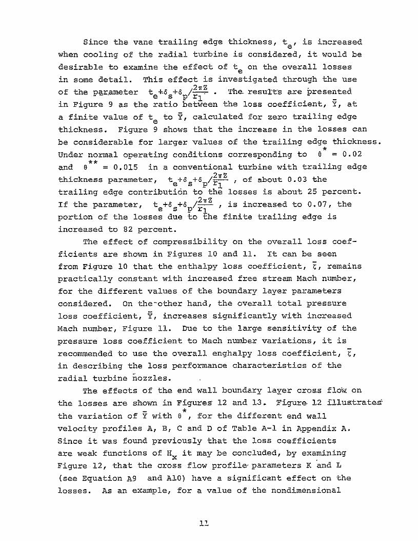
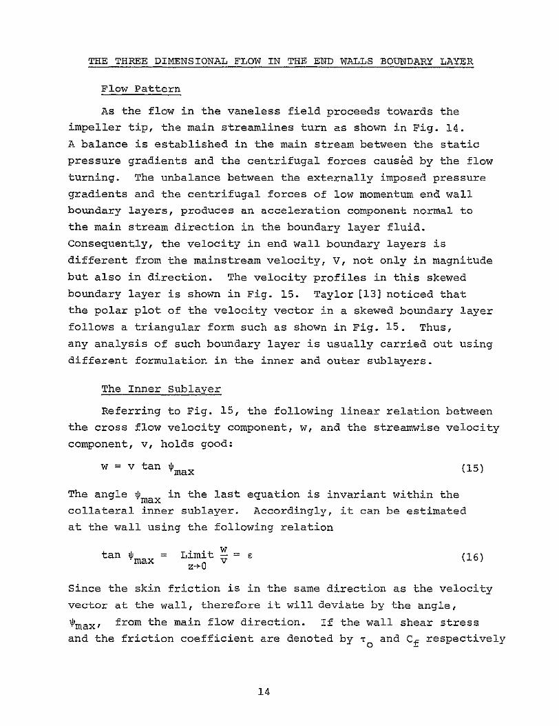
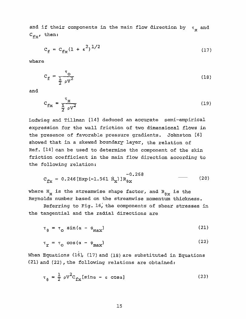
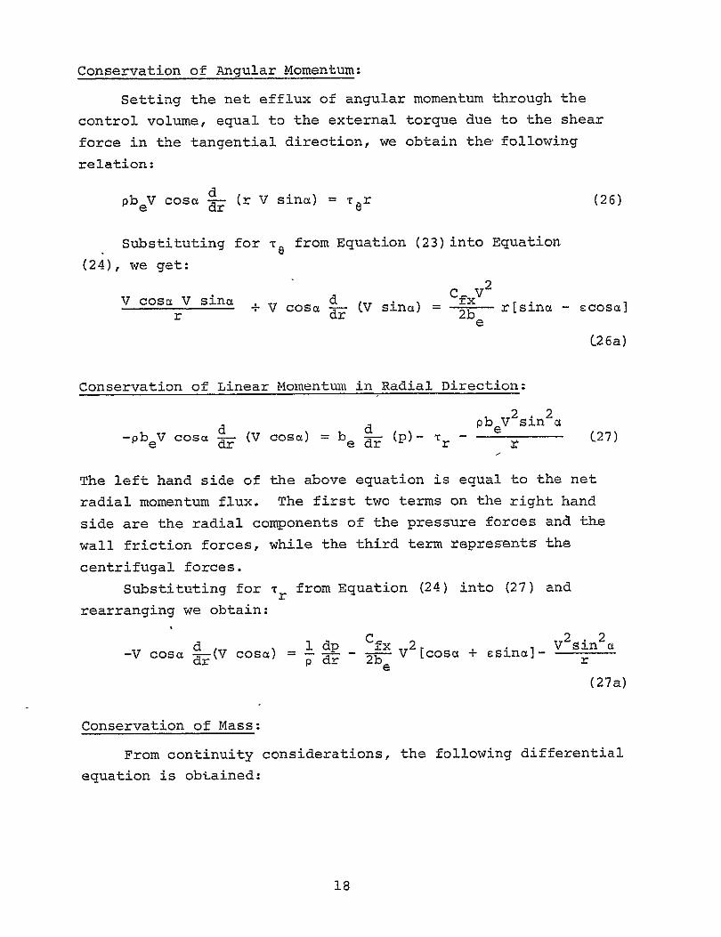
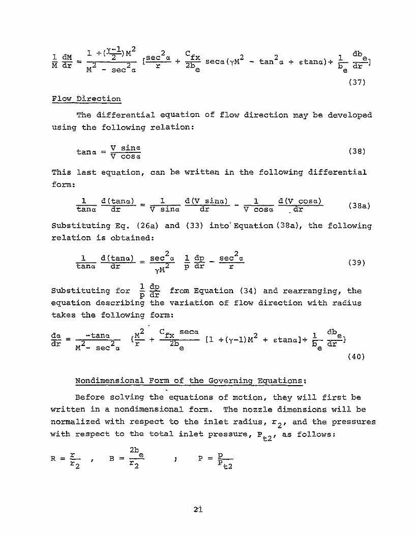
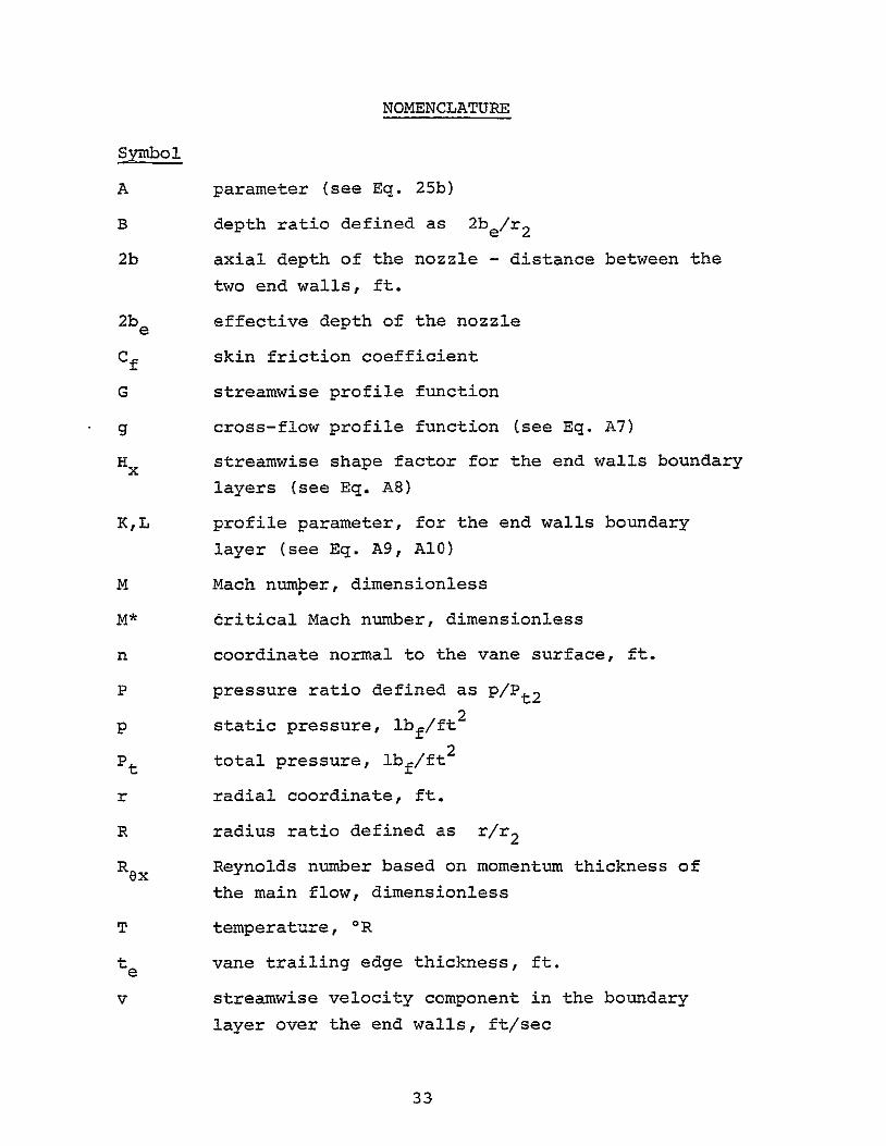
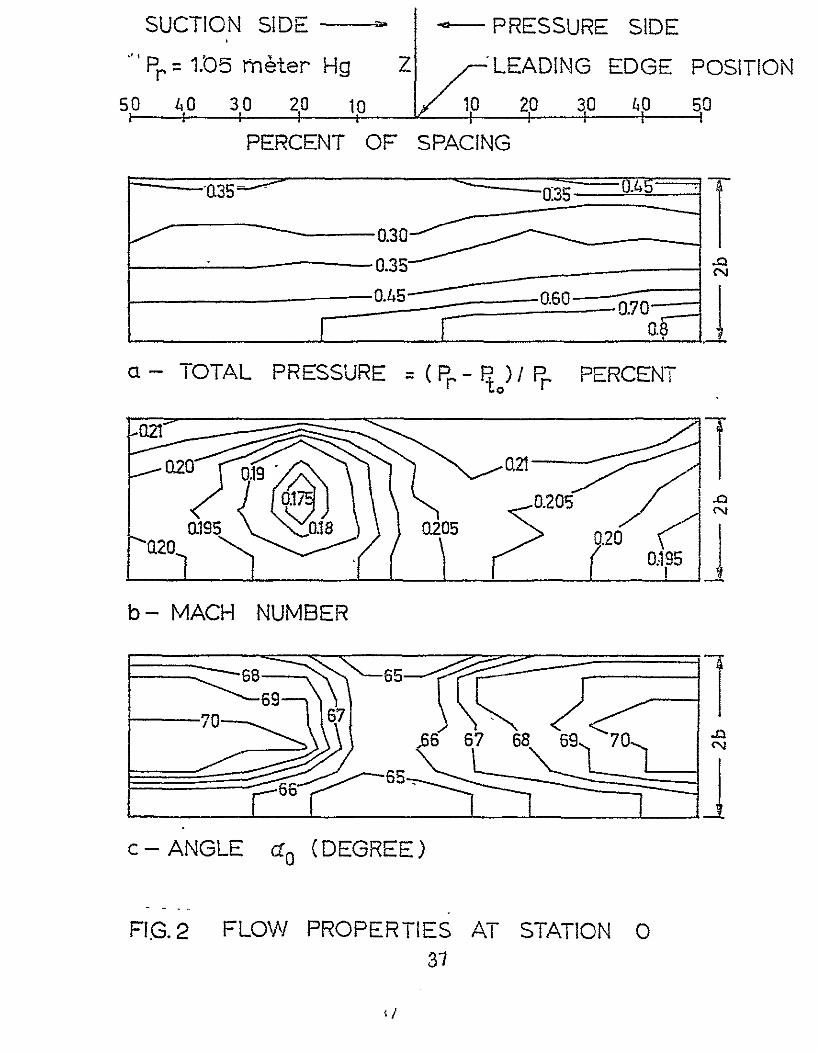
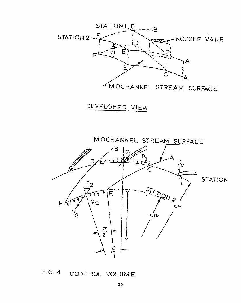

C
ANGULAR( te+CSs+3pD
018 )
SPACING
= 005
=277
c = 600 o18shy -zshy q
0416 0 004003
014shy0-030030-04 0-02
012shy 02 0-03 -0-03 002 -004001
w 001 003 5 010 002 0-02 L 003001
0 OB
001 002 002 1001
ul 006 0
5j 001 5001
004
a Hx 20 - 002-
I 0
0 02o 04 05 06 07 08 09 MACH NO
PIG1O VARIATION OF ENTHALPY LOSS
COEFFICIENT WITH MACH NO
45
04 amp03 022-
ANGULAR SPACING 277
020 (te+ s -) = 05 03amp03
r01 2 -IT0
04amp02
0-18shy a=60
-02 amp30
016shy 04 amp -01
0-14shy -1~ amp 03
Z X -02 amp 02 IL 03 amp -01 C) 012
u 00 amp -03
01 amp 02
0
0-0-Lo
amp01
bi
W 00shy 0020 amp00 -_ H00 amp20
I I I I0 02 04 06 0-8 1
MACH NO
FIG11 VARIATION OF PRESSURE LOSS
COEFFICIENT WITH MACH NO
46
Igt-
ANGULAR SPACING = 277 nw (t + +8 ) K e s p 0-O02
zshyui 0
-J cz=6 0
o Si z 0003 lt 025 - E 0=O3
020shy
0 00
I--deg
PROFILE LUi 010 - A
B 0 005-shy CU
D ()
0 0 001 002 003 004 005
NONDiMENSIONAL MOMENTUM THICKNESS e
FIG -12 EFFECT OF END WALLS PROFILE
PARAMETERS ON LOSS COEFFICIENT
47
ii
ANGULAR SPACING = 277 u)zw (t + pXe s P-00
w2 03 00
N60 0p 0
Z2 _
W 0358z
Nia6
z 010 031 0 II1
00 5-1
003 X
O0 K = 243 0L
K1 = 0966OW 00 3 00 =043
- 0NONDMEN SIONAL MOMENTUM THICKNESS 4-
FIG 13EFFECT OF END WALLS CROSS FLOW
PARAMETER (E)- ON LOSS COEFFICIENT
48
0
REFERENCE DIRECTION
VANELESS SPACE INLET
MAIN FLOW STREAMLINE
- - ROTOR TIP
-BOUNDARY LAYER STREAMLINE
FIG14FLOW PATH IN THE VANELESS FIELD
CROSS BL MAIN BL INNER OUTER zSUBLAYER SUBLAYER
-V - 1 --shy 2
V V V w
SxTx Tangent to maiflow str line 1
VV
a VELOCITY PROFILES b-VELOCTY POLAR PLOT
FIG 15 END WALL BOUNDARY LAYER
TANGENT TO MAIN FLOW STREAMLINE
SV sina TANGENTIAL DIRECTION
ul
F d
0 Co VELOCITY VECTOR u AT THE WALL
rY w
J
0
FIG 16 VELOCITY AND WALL SHEAR STRESS COMPONENTS IN THE SKEWED BOUNDARY LAYER
station
aMain stream line
---- 2 -2Ii -----
U1 U
-- R otor tip
FIG 17 VANELESS SPACE GEOMETRY AND COORDINATE
SYSTEMshy
STAT ION 2b
7- Illlll shy
2b L2 be
Vel oc ity Geometry Geometry Velocity d istri but ion distribution
a - Actual case b - Equivalent case
FIG 18 ACTUAL AND EOUIVALENT VANELESS SPACE GEOMETRY
-------------
do Developed view
4 dPdr
dr
Vsinct NLbe 2
FIG 19 CONTROL VOLUME
A
Mz=08
10 C
d
O 099
0 0-98-
Z2 d7Q
0J0-97 -
097
085 090 095 10 RADIUS RATIO R
FIG 20 EFFECT OF INLET FLOW ANGLE
55
15 20
T cS14 -2214o
a= 60
lt
ryIti Ld In
Z
13
12 07-z
a= 70
02--80
110
085
FIG 21
090 095 RADIUS RATIO R
EFFECT OF INLET FLOW ANGLE
10
56
M2 08
Ishyz 005shy
0 0
LL0 IL
0tamp0 u 003shy
a 2 =70
a = 600
0 -U 002
U) U)
0L
001 -
0
05 090 095 10
LLI~ pRADIUS- RATIO R
FIG 22fa- EFFECT OF INLET FLOW ANGLE
0M05shy 0
z
i -
0
0 a06
LU 002-S0101
Il ampI I 00
085 0-90 0-95 10 RADIUS RATIO R
FIG 22 b EFFECT OF INLET FLOW ANGLE
deg a= 70
110
C 099shy
-M = 12ci
0
D
098shy
lt Mz= 05
0 8
H z w
0
097
2lt 096shy
(9 z
095 085
I 090
RADIUS
-
095 RATIO R
10
FIG 23 EFFECT OF INLET MACH NUMBER
1 7019
r4- M222 12
-17
0 Ishy
D z 13 r10 M =0f
11
1 095 10 RADIUS RATIO R
FI G 24 EFFECT OF INLET MACH NUMBER
60
LW
0
0
0024 - M -05
M42=0s
M=12
a=700 _
Ishy
z 0008 w
085 090 RADIUS
095 RATIO R
10
FI G25 a EFFECT -OFINLET MACH NUMBER
003 shy
-- M2 05 ashy0
0
Igtshyz ~ -shy v2 08
z w 002
LUc0
0
Lu
D
U)c)
085 090 095 10
RADIUS RATIO R
FIG 25b EFFECT OF INLET MACH NUMBER
013
- 099shyc~
r 2b
o 0-98 -
Cshy
r2 -15
H
z
090(2b
0
0-96shy
5
0-8096951
RADIUS RATIO R
FIG 26 EFFOT OF END WALL SPACING
63
15
M =08
a= 70
2 14
2b
O Ishy
r 13
2b
-10
z 2
12shy
10 085 090 095 10
RADIUS RATIO R
FIG 27 EFFECT OF END WALL SPACING
64
M2 =01
I--a2 70 z
w 2b
_0 002 2 b
w 0
5 090 09b5 10
~RADIUS RATIO
FI G 28 a EFFECT OF END WALL SPACING
M =OB a0
a2 = 70
w 0 =15
0U 003shy2b
Oi 002 2 b
LU[
001 - -
Lii
0 --shy
085 090 095 10 RADIUS RATIO R
FIG 28 bEFRECT OF END WALL SPACING
APPENDIX A
FORMULATION OF RELATIONS BETWEEN INTEGRAL QUANTITIES
AND BOUNDARY LAYER CHARACTERISTIC PARAMETERS
Al Basic Relations and Definitions
In this Appendix the integrals which appear in the left
hand side of Eqs (2) (4) and (6) will be determined in terms
of the boundary layer characteristics at station 1 To
accomplish this the domain of integral will be divided into
a main stream region and boundary region as shown in Figure Al
This is a generalization of the approach used in the two
dimensional analysis of Reference [5]
At exit from the nozzle channels the profile boundary
layer developed along the vane surfaces is collateral while
the end wall boundary layer is skewed The velocity vectors
within the skewed boundary layer can hence be resolved into a
streamwise component v and a cross flow component w The
displacement and momentuim thicknesses are used to describe the
boundary layers at station 1 These two quantities for the
collateral boundary layer are defined as
f pxr dn (Al)(pv
f f= pV dn-f- 2 dn (A2)
o (pV) o (pV)
Where n is the coordinate normal to the vane surface and 6f
is the boundary layer thickness On the other hand the streamwise
and cross flow end wall boundary layer displacement and the
momentum thickness are defined as follows
6f ax =f - f pV dz (A3)
0 (PV)7
67
V (A4)x f=f (PV dz - SfI (P2PV dz
af6 = dz (AS)
af 0 = f pw 2 dz (A6)
o (pV 2 )
Where z is the coordinate normal to the end wall surface
The relation between the parameters of equations (A3) through
(A6) can be determined for a given boundary layer profile
It is assumed that in the end wall boundary layer the streamwise
and the cross flow velocity profiles are given by Reference [63
v__ = Gw - sG g (A7) Vfs fs
In the above equations G and g are functions of the coordinate
perpendicular to the end wall z normalized with respect to the
boundary layer thickness (Sf) 6Eis the tangent of the angle
between the surface shear and the local main flow direction
as shown in Fig A2
The following streamwise and cross flow parameters are
used to describe the end wall boundary layers using the assumed
formes of the velocity profiles
f
x 0 (-pG)dzx o x x f(A8)
f (I-G)G dz 0
68
f 5 P(Gg)dz
cec f (A9)
I (v-iG)G dz0
6f 2
If p(Gg) dz
L e c ex f
(Al0)
I (p-pG) (G)dz 0
Where v is the nondimensional ratio pp
In Ref [7] various families of functions G and g that aremost compatible with the experimental data were determined
The corresponding profiles are plotted in Fig A3 together
with the Band B of the experimental data obtained by
Johnson [6] The various parameters of Eqs (A12) (A13) and
(A14) were calculated for the incompressible flow corresponding
to the profiles of Fig A3 and are given in the following
table
Profile H K Lx
A 1286 0457 00359
B 137 243 0968
C 140 227 0989
D 1286 1249 0262
TABLE A-l TYPICAL VALUES FOR THE END WALL BOUNDARY LAYER
CHARACTERISTIC PARAMETERS
69
A2 Evaluation of the Different Integral Terms in the
Governing Equations
The integrals in the Governing Equations (2) (4) and (6)
will be expressed in terms of the boundary layer parameters of
Eqs (Al) through (A10) based on the following assumptions
1 Different boundary layers do not interfere with
each other hence corner effects are neglected
2 The flow is homogeneous outside the boundary
layer regions at exit from the nozzle channels
In accordance with the foregoing assumption the velocity
distribution of Figure A3 due to the profile boundary layers
on the vane surfaces will result in the variation of the total
pressure in the tangential direction shown in Figure A4 The
total pressure and velocity deficiencies in the axial direction
caused by the end wall boundary layers will be similar to those
indicated in Figures A5 and A6
Referring to Figure A2 the following equations relate
the different skewed end wall boundary layer velocity components
and flow angles
V cosa = v cosa 1 + w sina1 (A12)
V 2 2 2cosa sina = v cosa sina1 - w cosl sinam (A13)
V2and cos2 may be approximated by
V2 c~2 2 2 22SCos = v cos aI + w sin2l (A14)
Where a is the angle between the flow direction and the radial
inward direction as before while a1 is the same angle for
the local free stream at station 1 which is independent of z
and a according to the assumptions
70
+b +7rZA21 Evaluation of the Integral I [ f (p Vr cosa) 1de]dz
-b -iZ
Referring to Figure Al it is more convenient to breakup
the above integration into three separate integrals as follows
+b +rZ +b-Suf +wZf [ (pVr cosa)ide]dz - cosair1 f f (PV) idedz
-b -nZ -b+6kz -nZ
-b+6f +7FZ b +7rZ
+ rI I [ f (pV cosa)1d8]dz + f [ f (pV cosa)ide]dz-b -wZ b-uf -Zf (A15)
where
6uf 6Af are the full boundary layer thicknesses over
the upper and lower end wall surfaces
Referring to Figure A2 the coordinate used in the profile
boundary layer equations is related to the circumferential
coordinate 0 by
da = r n (Al6)r1cosa1
Substituting the above expression for de in the first term in
the right hand side of equation (Al5) and using the definition
of the displacement thickness of Equation (Al) we can arrive
at
+b-6 u
[ (PV)ld]dz = [2b -(6u + 6)]pV)l 2 -ta-e e I ~ ~f~ ~ fP ztzf
(Al7)
where
S(6 s + 0p)- r1 cOSu 1 (Al8)
-ste=te2 rl cosal (A19)
71
and
as 6p are the boundary layer displacement thickness
over suction and pressure surfaces of the vane
te is the vane trailing edge thickness
2_ is the angular spacing between two successive
vanes
Using Eq (A12) the last two terms on the right hand side of
Equation (A15) could be rewritten as
-b++b+b +7rZf f +WZ
( f (pV cosc)ide]dz + I E f (pV Cosc) ldeldz -b -IrZ +b-6 -wZUf
2r b+Co p (v + w tan 1 )
cosa[1 _fPV) pV) dz
+b p(v + w tanI1 )+b- f (PV)1 dz]+b-6 uf 1p)
When Equations (A3) and (A5) are used the above equation
reduces to
-b+6yf +Z +b +wZ
f I (pV cosa) 1d0]dz + I [ (pV Cosa)Ido]dz-b -wZ +b-6uf -aZ
27r CV) 1 rlcosa (a+ a-(6 +6 )+(6 +6 )tan] (A20) k[a 6u Lx tx pound0 Cuf J)
where
ax 6ux are the streamwise boundary layer displacement
thicknesses over the lower and upper end walls
respectively shy
a cI auc are the cross flow boundary layer displacement
thicknesses over the lower and upper end walls
respectively
72
Finally substituting Equations (A17) and (A20) into (A15)
we get
+b irZ 2r E f (pVr cosc)ide]dz = (pV) (Z-)rlCosa 1
2b- (6u +6k)I [shy-b TZ f f
[1- -6te ]+[69f+uf -(Zx+ux)+(6c+ uc)tanail (A21)
If we define the following nondimensional parameters
2bux+Zx (A22)
x Hx - K tana1 (A23)
where
aux a are the streamwise boundary layer momentum
thicknesses over the upper and lower end
walls respectively
Equation (A21) can be simplified by neglecting the higher
order terms (6uf + 66 (u -+-dkf)6te and introducing
the parameters defined by equations (A) (A9) (A22) and (A23)
giving the following relation
+b + Z 2-u I [ I (pVr cosa) 1deldz = (pV)= r r1cosa I 2b[1-6 -6te- ]G0 -b - Z 1 (A24)
+b +rZ 2 2A22 Evaluation of the Integral I [ I Cr pV cosasina)1 d8]dz
-b -irZ
The evaluation of the integral will be divided over the
three same regions discussed previously
73
+b +wZ 2 2 2f [ (r pV coscsina)1jd]dz = r1 cosalsinal [2b shy
-b -nZ
+rZa 2 d+2 2-b+6f 2 -6]Yp (PI 2 r 2) (pV cosasinc) dzf f -irZ -b
b 2(A5 asina) d z ] + I (pV cos (A25)
b-6 uf
Using Eqs (Al) (A2) and (Al6) into the first term in
the right hand side of Eq (A25) it reduces to
r2 cosaisina 11[2b - (6u + a )t I (pV 2 ) 1 de 1 Uf Z -Z
cs]1[2b-[-OS-+e-(pV2) sina cosa [2b-(6 )]2 r2 [1-66 3 (A26) u f z 1te
where
(s + 8p)fZ-rl cosaI (A27)
and
es and 6p are the boundary layer momentum thickness onthe vane suction and pressure surfaces
respectively
When Eqs (Al3) (A4) and (A6) are substituted into the second
and third term of (A25) it can be deduced that
-b+S shy
f (cosasina pV2 )dz = (pV2 cosa1 sinalljSf-6tx-8Px-ezc ]-b
(A28)
74
and
f (coscsina pV2)idz = (pV2 cosisinl[6uf-6ux-6ux-8uc] uf (A29)
where
8uc and 8Zc are the cross flow boundary layer momentum
thickness over the upper and lower end walls
respectively
Finally substituting Equations (A26) (A28) and (A29) into
(A25) and making use of the parameters given by (AS) and (Al)
the integral of equation (4) is expressed as follows
+b +iZ 2 2 2 2n 2 f [ f (r pV cosasin) 1 de]dz = (pV )I sinacosa1 --riI 2b
-b -rZ
[l- - te - e - ne] (A30)
where
n=1 + H + 2 L (A31)
+b +rZ 2
A23 Evaluation of the Integral _f X (pV cosa rcos(a+8)1dedz-b -wZ
Using trigometric relations the above integral may be
expanded as follows
+b +rZ 2 +b +Z 2 2 f f (pV r cosacos(a+8) 1deldz = f[ (pV r cos a) 1cos8d9]dz -b -nZ -b -nZ
+b +rZ 2 - f E (pV r coscsina)1 sinedejdz (A32)
-b -rZ
The first integral in the right hand side of Equation (A32)
may be rewritten as
75
+Ib +wZ 2 2 2+b If(pV r cos a) cosa de]dz = r1cos all - shy
-b -wz 1f
+Z +wZ -b+6f 2 2 -f -Z (pv )lCOSede + r I f E- (pV cos a)1cosedz]de
f 7T-ir2 -b
+wrZ b 2 2(A3 + f [I (pV cosa2) cosedzidel (A33)
-wZ b-S 1
For unseparated flows the angular coordinate 0 does
not change appreciably inside the boundary layers formed over
the vane surfaces Consequently 8 can be considered equal
to the angular spacing wZ within these boundary layer
regions Using this value of 6 together with Equation (A2)
it can be easily deduced that
-I-wZ 2 2 c 8 + P + +7Tz I (pV2)icosede = -(pV2) Cos + V( - pV)cosd
1 Z r1Cosa I1-wZ
(A34)
Using the definition of the displacement thickness given by Equation
(Al) the second term in the right hand side of Equation (A34)
reduces to+7wz-27rpV 1sin uZ _Cs7f (PV)Icosede = 2w si rZ- 00s Y ( + te)] (A35)
ol Z t
If Equation (A35) is substituted into (A34) the following relation
can be written
_wrzV2 cosede = 2-(pV2 sin Z - cos (amp + a +
f(pV zl pound TZ Zte (A36)
Using Equations (A14) (A4) and (A) the integrals in the right
hand side of (A33) reduce to
76
+7rZ -b+af 2 2 7r 2 2f f (pV cos a)lCose dzdo = 2sin f cos a1 (pV
-1rZ -b I f
- SX - ekx + k tan 2c I) (A37)
+7r Z +b 2 2 7sn 2 2shyf f (pV cos 2 ) 1cosedzde 2sin C s2 l(pV2V (S shy
-7iZ +b-k fuf
-a -Ou + a tan2a I) (A38)
Substituting Equations (A36) (A37) and (A38) into the right hand
side of (A33) we arrive at
+b +Z 2 22 2 2i I f I (pV r cos a) cosede]dz = 2b r)Cos a VI)z1 -b -nZ 1
- 8 (1 + Hx - s2L tan2a)] - cos 2 ( + + ) (A39)x z te
where Hx pound2L are given by the Equations (AS) and (AI0)Following a procedure similar to the one used to obtain equation
(A39) it may be easily deduced that
+b +w2+b I (pV
2r cosasina)1 sinede]dz = 0 (A40)
-b -rZ
Finally substituting Equations (A39) (A40) into (A33) therequired value of the integral in Equation (6) is obtained as
+b [pV COSa rcos(ct+O)]ldodz = 2b(pV2) cos2a 27r-b -wZ c- 1
sin
( -r )- T ( + ate + e )] (A4)
77
where
= +H x L tan2l (A42)
Equations (A24) (A30) and (A41) will be used in equations
(2) (4) and (6) to express the continuity the angular momentum
and the linear momentum equations in terms of the boundary
layer characteristic parameters at station 1
78
MAIN FLOW REGION
Sul te
LSKEWED END WALL B L
COLLATERAL PROFILE BLa = )
FIG A-i FLOW REGIONS AT EXIT FROM THE NOZZLE CHANNEL
MAIN FLOW STREAMLINE
END WALL BOUNDARY LAYER STREAML-INE
co
FIGA-2 NOMENCLATURE AND SYMBOLS AT VANES-TRAILING EDGE
07
C
05-D -B
03shycc
HA
01
02 04 0 10 G
FIG A-3 NORMALISED CROSS FLOW PROFILES
5sf 6 pf
cosa cosa 1
I
r~-K te -Zr c0S G(
FIG-A-4 TYPICAL VELOCITY DISTRIBUTION IN CIRCUMFERETIAL DIRECTION AT NOZZLE EXIT
p t o p i p
W r __ __ r 2cos aZ
FIGA-5 TYPICAL PRESSURE DISTRIBUTION IN CIRCUMFERENTIAL DIRECTION AT NOZZLE EXIT
82
UPPER SURFACE LOWER SURFACE
6 Uf 161f
P tfsi Po
+b o -b
FIGA-6 TYPICAL TOTAL PRESSURE DrSTRIBUTION IN AXIAL DIRECTION AT NOZZLE EXIT
~2b-6uf -61f
Vfs1
+b I-b 0
FIG A-7 TYPICAL VELOCITY DISTRIBUTION IN AXIAL DIRECTION AT NOZZLE EXIT
v gt171
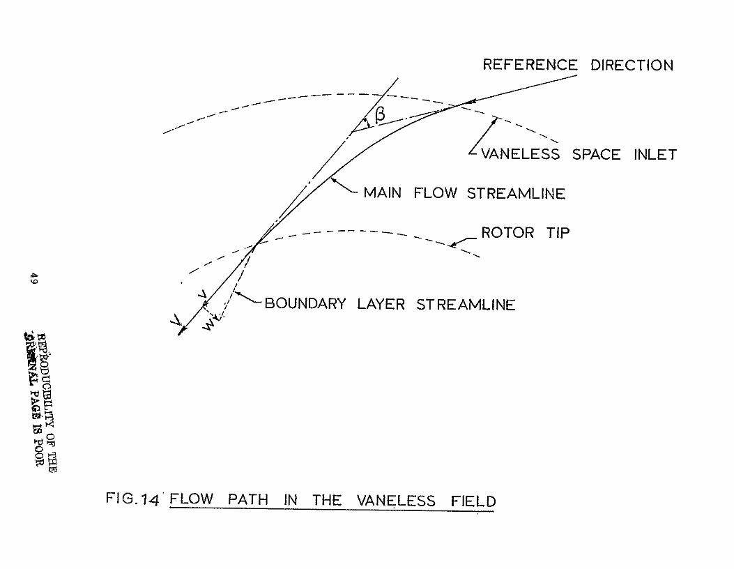
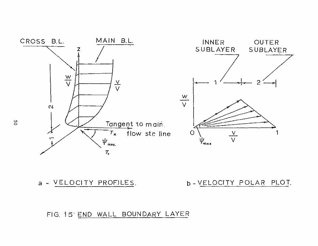
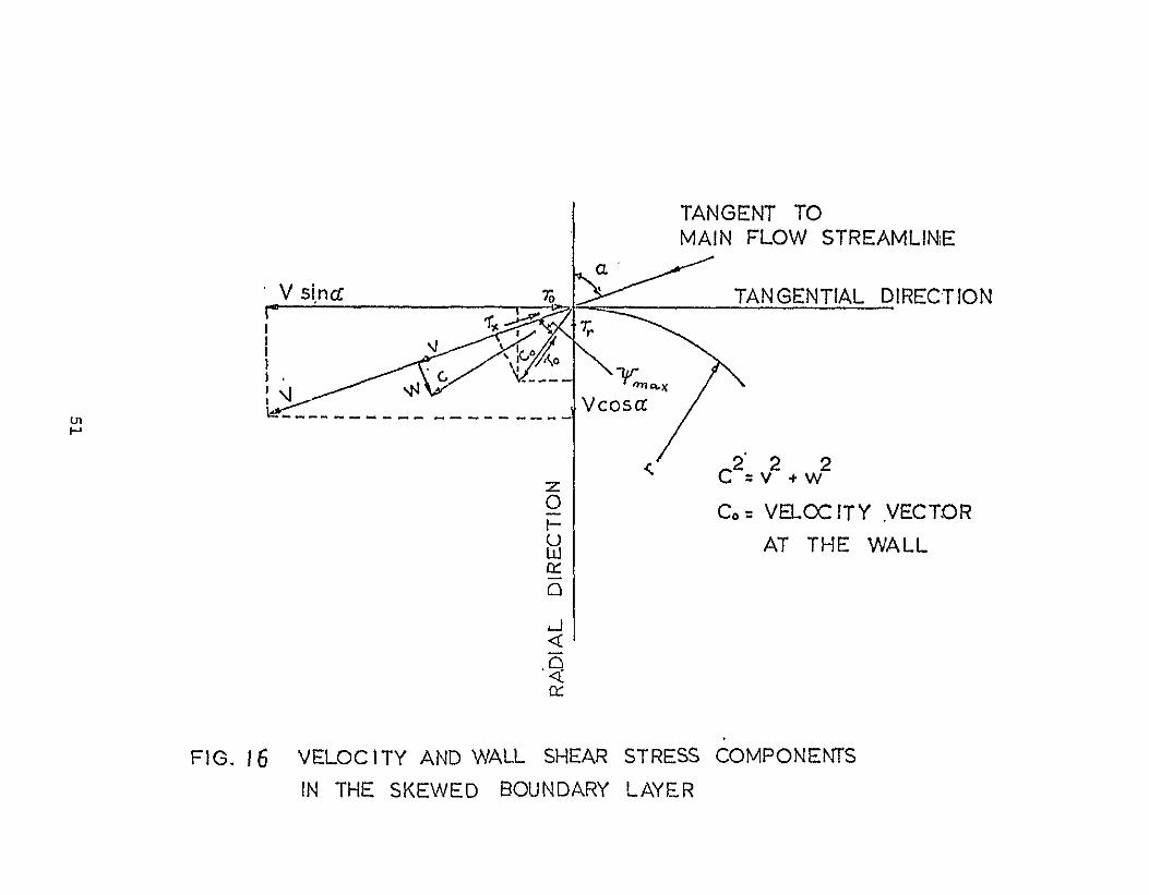
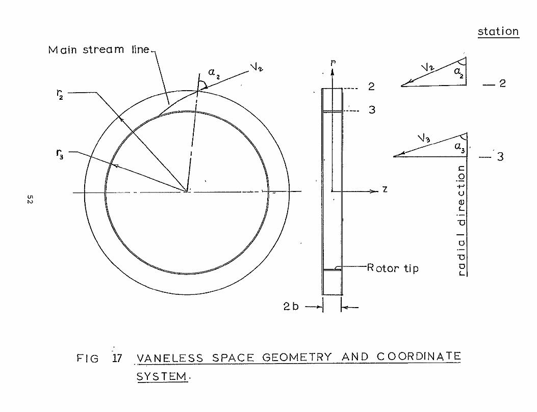
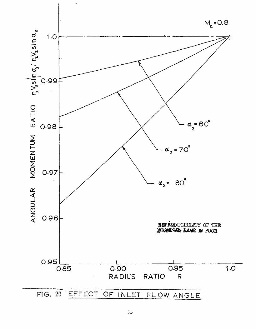
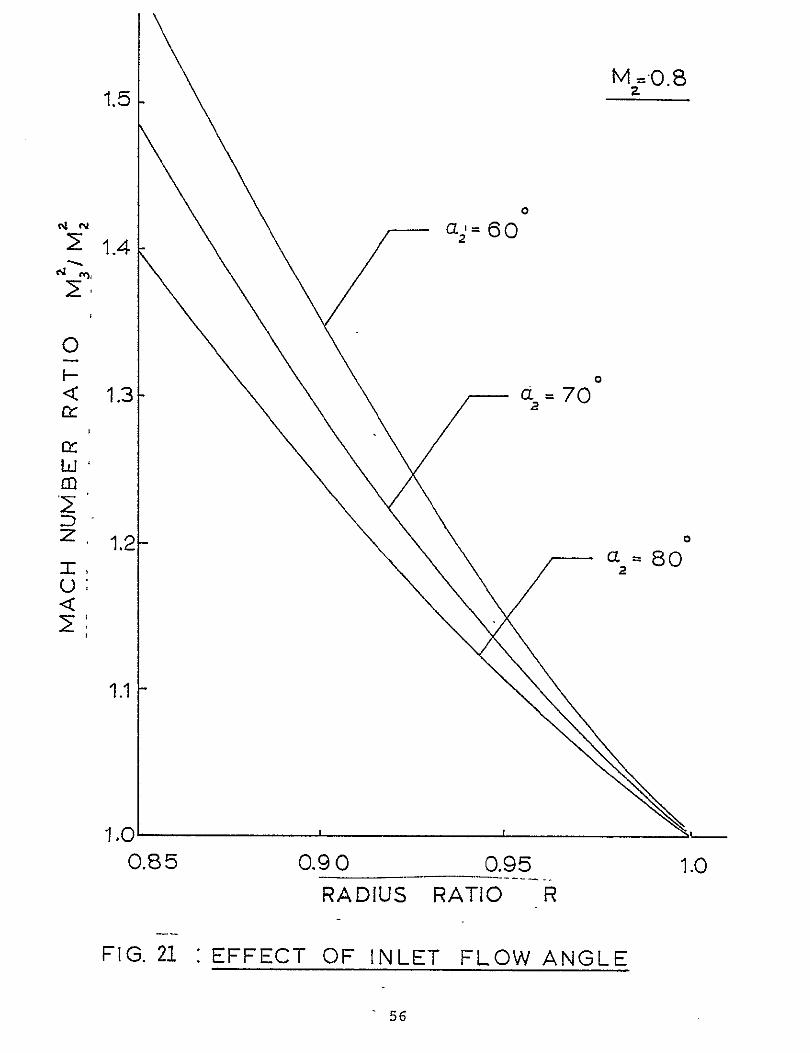
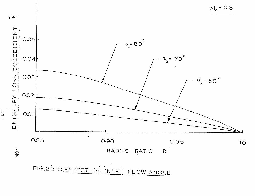
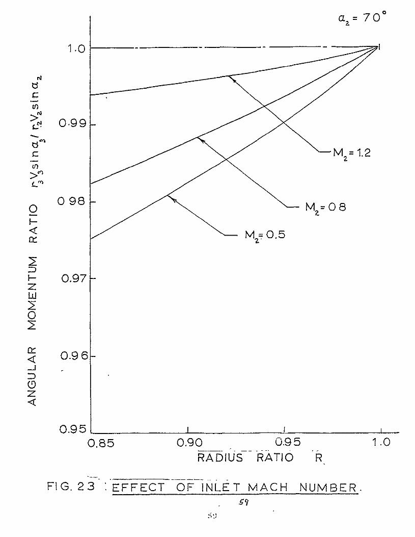
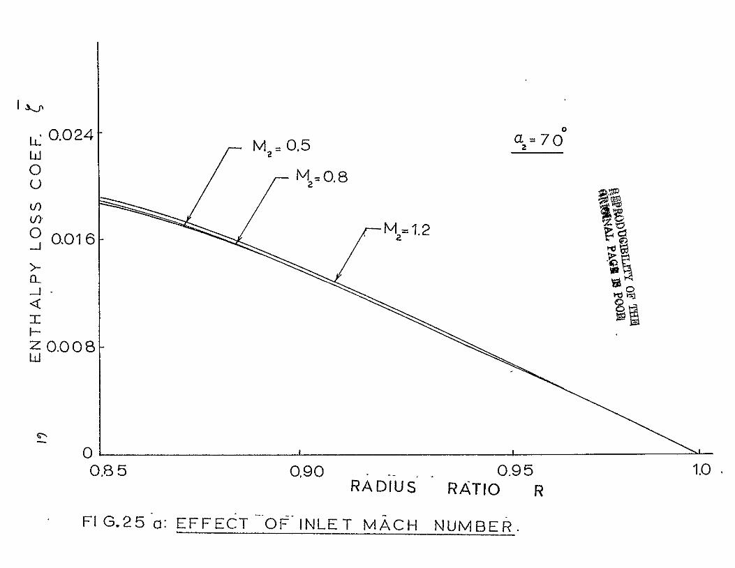
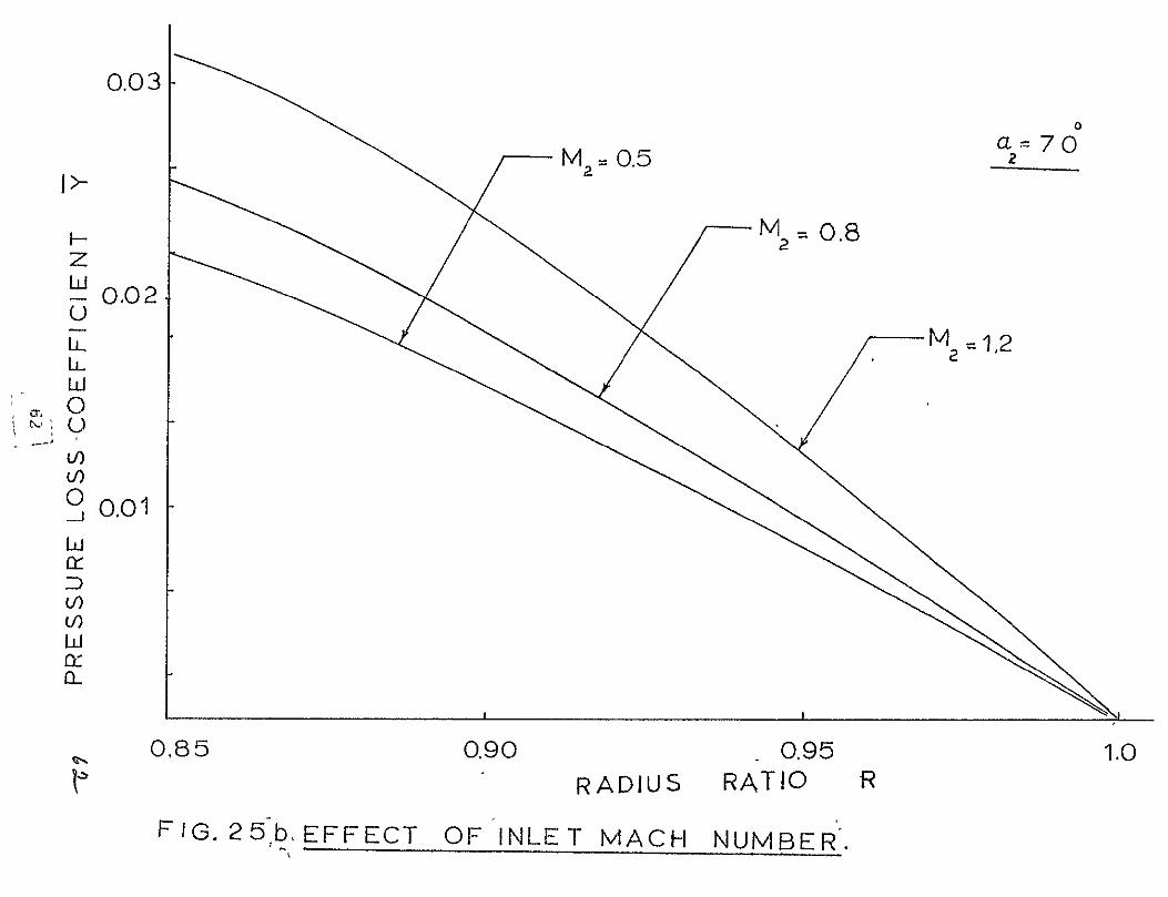
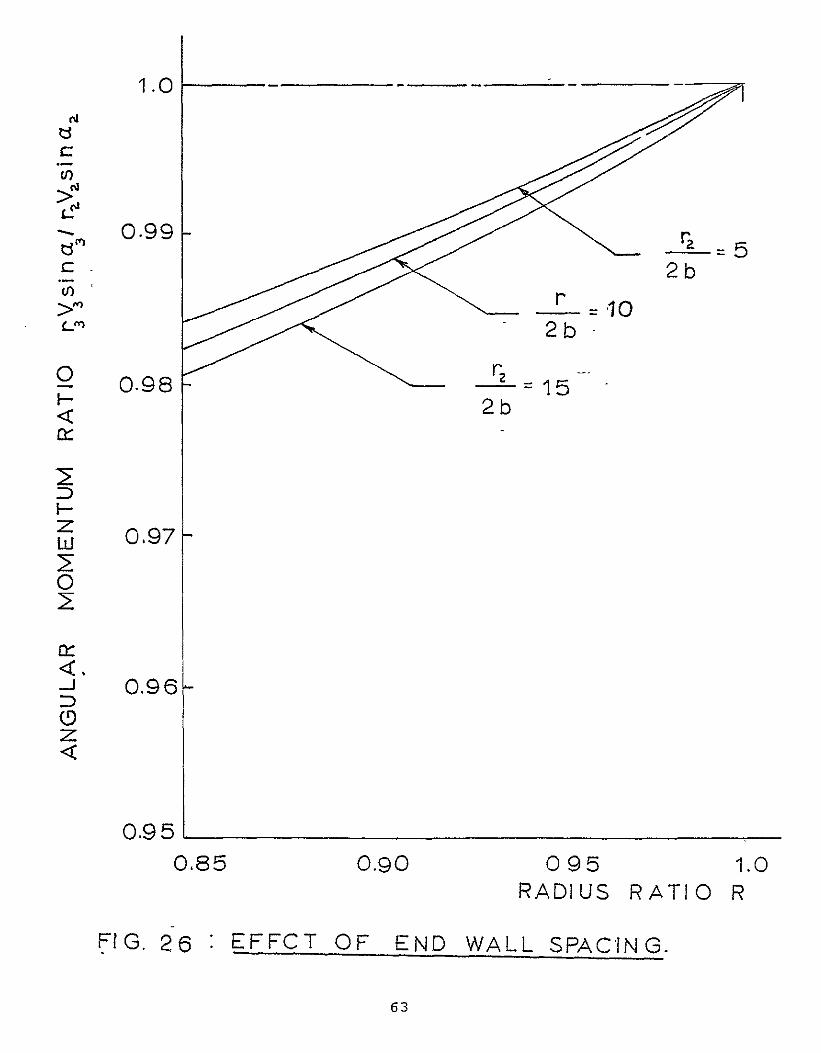
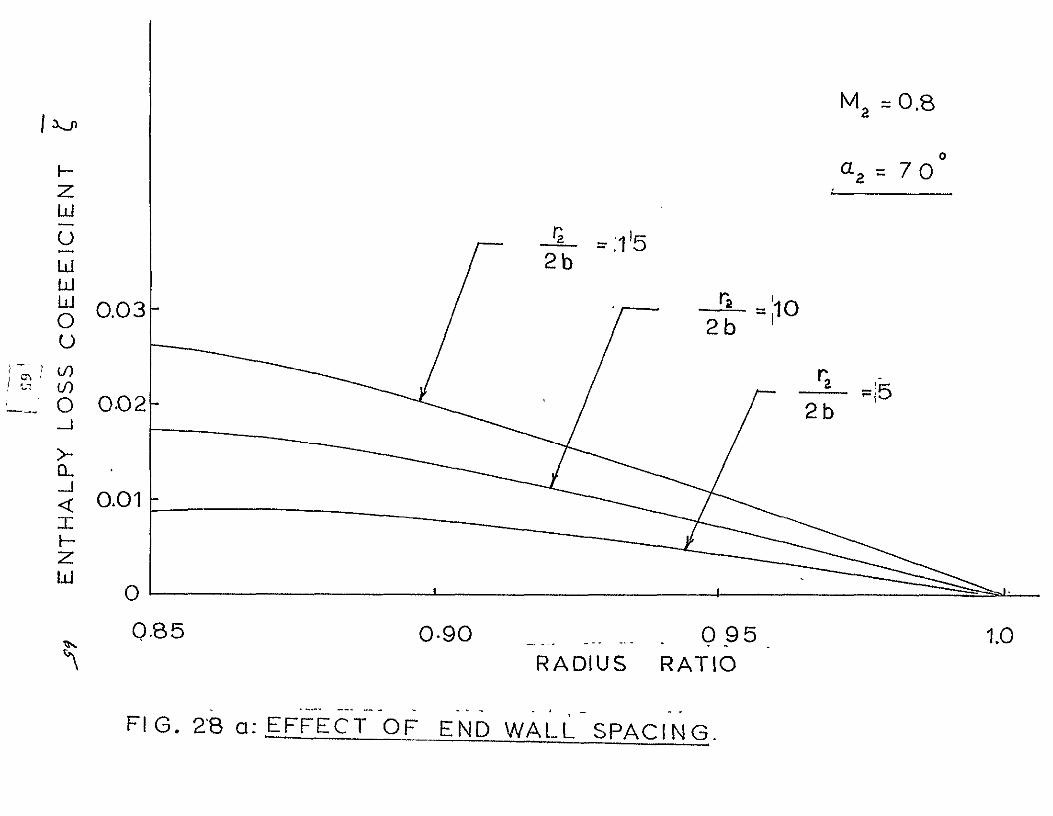
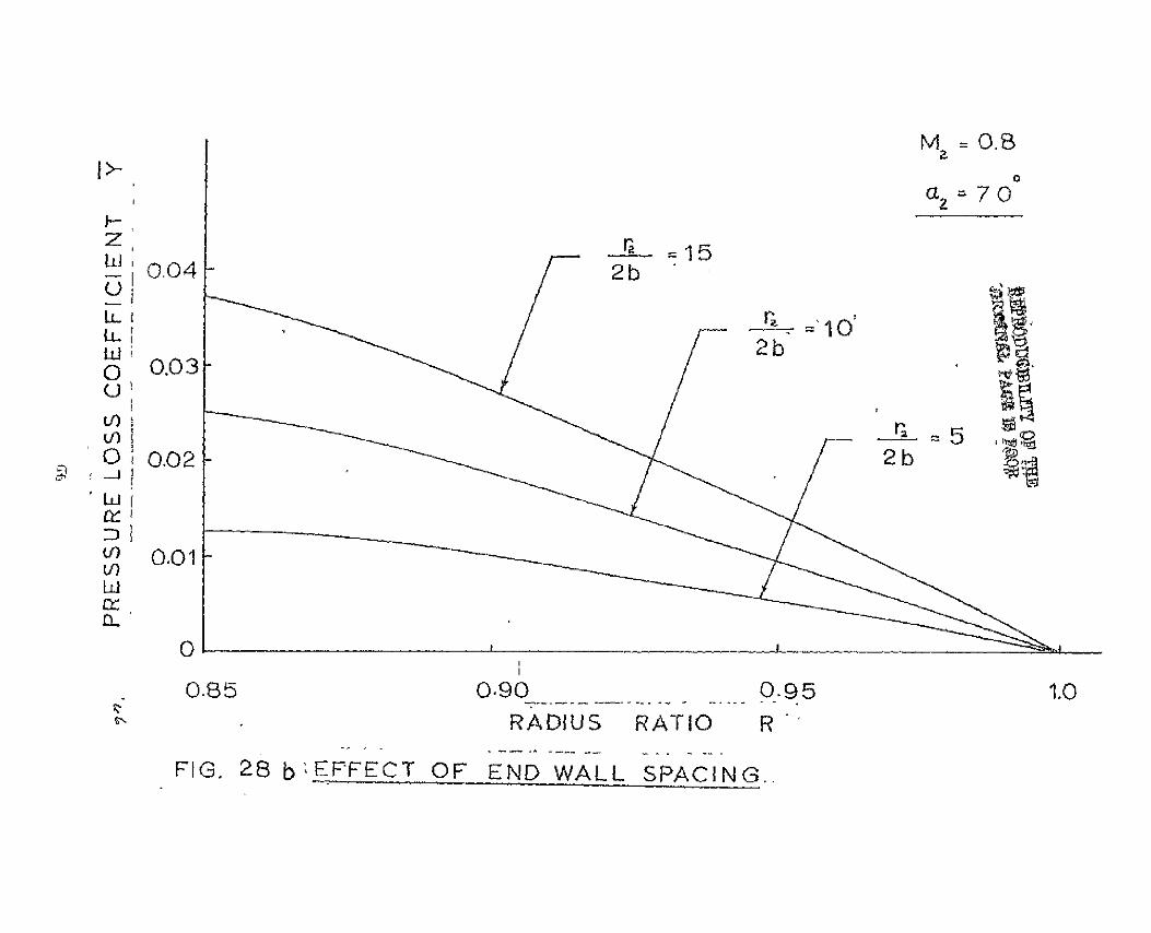
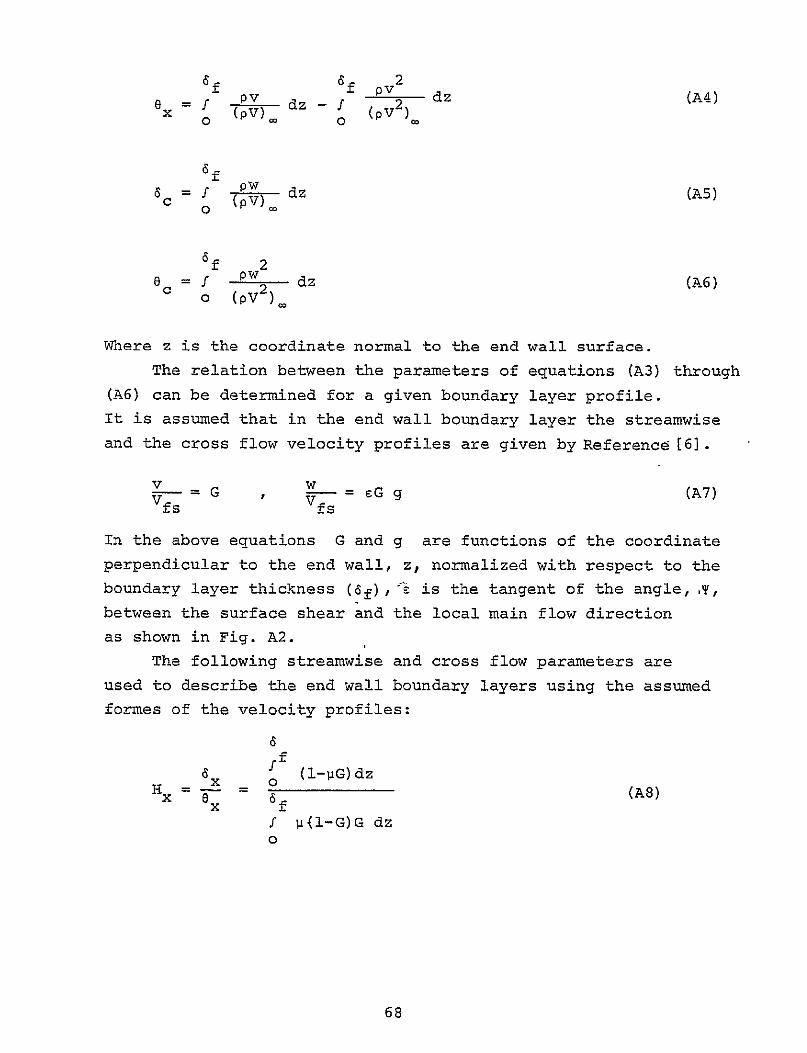
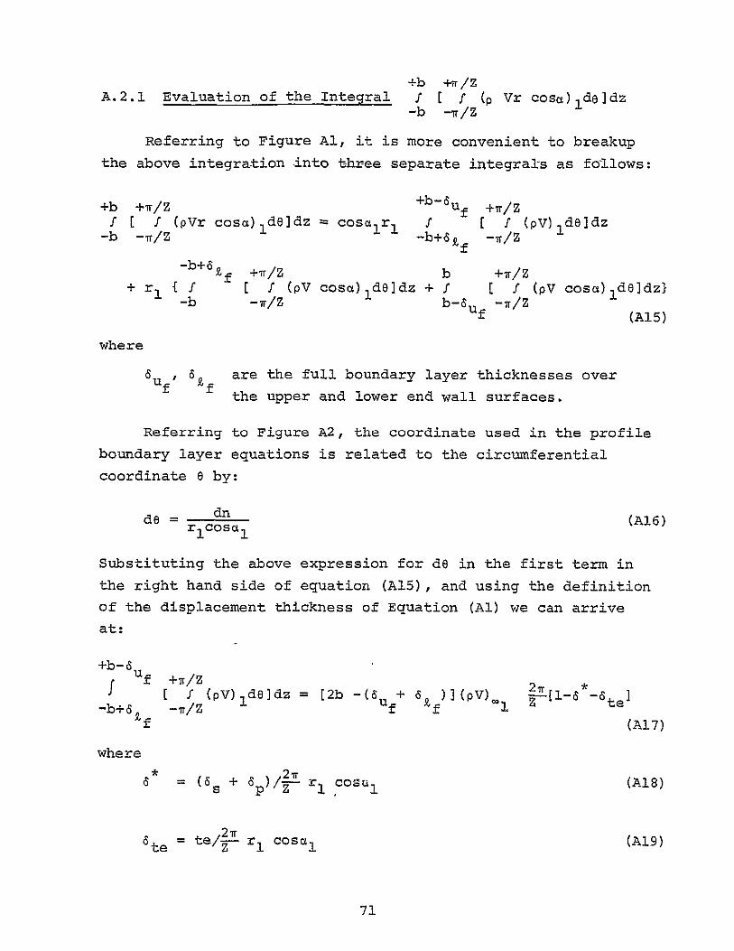
and
as 6p are the boundary layer displacement thickness
over suction and pressure surfaces of the vane
te is the vane trailing edge thickness
2_ is the angular spacing between two successive
vanes
Using Eq (A12) the last two terms on the right hand side of
Equation (A15) could be rewritten as
-b++b+b +7rZf f +WZ
( f (pV cosc)ide]dz + I E f (pV Cosc) ldeldz -b -IrZ +b-6 -wZUf
2r b+Co p (v + w tan 1 )
cosa[1 _fPV) pV) dz
+b p(v + w tanI1 )+b- f (PV)1 dz]+b-6 uf 1p)
When Equations (A3) and (A5) are used the above equation
reduces to
-b+6yf +Z +b +wZ
f I (pV cosa) 1d0]dz + I [ (pV Cosa)Ido]dz-b -wZ +b-6uf -aZ
27r CV) 1 rlcosa (a+ a-(6 +6 )+(6 +6 )tan] (A20) k[a 6u Lx tx pound0 Cuf J)
where
ax 6ux are the streamwise boundary layer displacement
thicknesses over the lower and upper end walls
respectively shy
a cI auc are the cross flow boundary layer displacement
thicknesses over the lower and upper end walls
respectively
72
Finally substituting Equations (A17) and (A20) into (A15)
we get
+b irZ 2r E f (pVr cosc)ide]dz = (pV) (Z-)rlCosa 1
2b- (6u +6k)I [shy-b TZ f f
[1- -6te ]+[69f+uf -(Zx+ux)+(6c+ uc)tanail (A21)
If we define the following nondimensional parameters
2bux+Zx (A22)
x Hx - K tana1 (A23)
where
aux a are the streamwise boundary layer momentum
thicknesses over the upper and lower end
walls respectively
Equation (A21) can be simplified by neglecting the higher
order terms (6uf + 66 (u -+-dkf)6te and introducing
the parameters defined by equations (A) (A9) (A22) and (A23)
giving the following relation
+b + Z 2-u I [ I (pVr cosa) 1deldz = (pV)= r r1cosa I 2b[1-6 -6te- ]G0 -b - Z 1 (A24)
+b +rZ 2 2A22 Evaluation of the Integral I [ I Cr pV cosasina)1 d8]dz
-b -irZ
The evaluation of the integral will be divided over the
three same regions discussed previously
73
+b +wZ 2 2 2f [ (r pV coscsina)1jd]dz = r1 cosalsinal [2b shy
-b -nZ
+rZa 2 d+2 2-b+6f 2 -6]Yp (PI 2 r 2) (pV cosasinc) dzf f -irZ -b
b 2(A5 asina) d z ] + I (pV cos (A25)
b-6 uf
Using Eqs (Al) (A2) and (Al6) into the first term in
the right hand side of Eq (A25) it reduces to
r2 cosaisina 11[2b - (6u + a )t I (pV 2 ) 1 de 1 Uf Z -Z
cs]1[2b-[-OS-+e-(pV2) sina cosa [2b-(6 )]2 r2 [1-66 3 (A26) u f z 1te
where
(s + 8p)fZ-rl cosaI (A27)
and
es and 6p are the boundary layer momentum thickness onthe vane suction and pressure surfaces
respectively
When Eqs (Al3) (A4) and (A6) are substituted into the second
and third term of (A25) it can be deduced that
-b+S shy
f (cosasina pV2 )dz = (pV2 cosa1 sinalljSf-6tx-8Px-ezc ]-b
(A28)
74
and
f (coscsina pV2)idz = (pV2 cosisinl[6uf-6ux-6ux-8uc] uf (A29)
where
8uc and 8Zc are the cross flow boundary layer momentum
thickness over the upper and lower end walls
respectively
Finally substituting Equations (A26) (A28) and (A29) into
(A25) and making use of the parameters given by (AS) and (Al)
the integral of equation (4) is expressed as follows
+b +iZ 2 2 2 2n 2 f [ f (r pV cosasin) 1 de]dz = (pV )I sinacosa1 --riI 2b
-b -rZ
[l- - te - e - ne] (A30)
where
n=1 + H + 2 L (A31)
+b +rZ 2
A23 Evaluation of the Integral _f X (pV cosa rcos(a+8)1dedz-b -wZ
Using trigometric relations the above integral may be
expanded as follows
+b +rZ 2 +b +Z 2 2 f f (pV r cosacos(a+8) 1deldz = f[ (pV r cos a) 1cos8d9]dz -b -nZ -b -nZ
+b +rZ 2 - f E (pV r coscsina)1 sinedejdz (A32)
-b -rZ
The first integral in the right hand side of Equation (A32)
may be rewritten as
75
+Ib +wZ 2 2 2+b If(pV r cos a) cosa de]dz = r1cos all - shy
-b -wz 1f
+Z +wZ -b+6f 2 2 -f -Z (pv )lCOSede + r I f E- (pV cos a)1cosedz]de
f 7T-ir2 -b
+wrZ b 2 2(A3 + f [I (pV cosa2) cosedzidel (A33)
-wZ b-S 1
For unseparated flows the angular coordinate 0 does
not change appreciably inside the boundary layers formed over
the vane surfaces Consequently 8 can be considered equal
to the angular spacing wZ within these boundary layer
regions Using this value of 6 together with Equation (A2)
it can be easily deduced that
-I-wZ 2 2 c 8 + P + +7Tz I (pV2)icosede = -(pV2) Cos + V( - pV)cosd
1 Z r1Cosa I1-wZ
(A34)
Using the definition of the displacement thickness given by Equation
(Al) the second term in the right hand side of Equation (A34)
reduces to+7wz-27rpV 1sin uZ _Cs7f (PV)Icosede = 2w si rZ- 00s Y ( + te)] (A35)
ol Z t
If Equation (A35) is substituted into (A34) the following relation
can be written
_wrzV2 cosede = 2-(pV2 sin Z - cos (amp + a +
f(pV zl pound TZ Zte (A36)
Using Equations (A14) (A4) and (A) the integrals in the right
hand side of (A33) reduce to
76
+7rZ -b+af 2 2 7r 2 2f f (pV cos a)lCose dzdo = 2sin f cos a1 (pV
-1rZ -b I f
- SX - ekx + k tan 2c I) (A37)
+7r Z +b 2 2 7sn 2 2shyf f (pV cos 2 ) 1cosedzde 2sin C s2 l(pV2V (S shy
-7iZ +b-k fuf
-a -Ou + a tan2a I) (A38)
Substituting Equations (A36) (A37) and (A38) into the right hand
side of (A33) we arrive at
+b +Z 2 22 2 2i I f I (pV r cos a) cosede]dz = 2b r)Cos a VI)z1 -b -nZ 1
- 8 (1 + Hx - s2L tan2a)] - cos 2 ( + + ) (A39)x z te
where Hx pound2L are given by the Equations (AS) and (AI0)Following a procedure similar to the one used to obtain equation
(A39) it may be easily deduced that
+b +w2+b I (pV
2r cosasina)1 sinede]dz = 0 (A40)
-b -rZ
Finally substituting Equations (A39) (A40) into (A33) therequired value of the integral in Equation (6) is obtained as
+b [pV COSa rcos(ct+O)]ldodz = 2b(pV2) cos2a 27r-b -wZ c- 1
sin
( -r )- T ( + ate + e )] (A4)
77
where
= +H x L tan2l (A42)
Equations (A24) (A30) and (A41) will be used in equations
(2) (4) and (6) to express the continuity the angular momentum
and the linear momentum equations in terms of the boundary
layer characteristic parameters at station 1
78
MAIN FLOW REGION
Sul te
LSKEWED END WALL B L
COLLATERAL PROFILE BLa = )
FIG A-i FLOW REGIONS AT EXIT FROM THE NOZZLE CHANNEL
MAIN FLOW STREAMLINE
END WALL BOUNDARY LAYER STREAML-INE
co
FIGA-2 NOMENCLATURE AND SYMBOLS AT VANES-TRAILING EDGE
07
C
05-D -B
03shycc
HA
01
02 04 0 10 G
FIG A-3 NORMALISED CROSS FLOW PROFILES
5sf 6 pf
cosa cosa 1
I
r~-K te -Zr c0S G(
FIG-A-4 TYPICAL VELOCITY DISTRIBUTION IN CIRCUMFERETIAL DIRECTION AT NOZZLE EXIT
p t o p i p
W r __ __ r 2cos aZ
FIGA-5 TYPICAL PRESSURE DISTRIBUTION IN CIRCUMFERENTIAL DIRECTION AT NOZZLE EXIT
82
UPPER SURFACE LOWER SURFACE
6 Uf 161f
P tfsi Po
+b o -b
FIGA-6 TYPICAL TOTAL PRESSURE DrSTRIBUTION IN AXIAL DIRECTION AT NOZZLE EXIT
~2b-6uf -61f
Vfs1
+b I-b 0
FIG A-7 TYPICAL VELOCITY DISTRIBUTION IN AXIAL DIRECTION AT NOZZLE EXIT
v gt171

UPPER SURFACE LOWER SURFACE
6 Uf 161f
P tfsi Po
+b o -b
FIGA-6 TYPICAL TOTAL PRESSURE DrSTRIBUTION IN AXIAL DIRECTION AT NOZZLE EXIT
~2b-6uf -61f
Vfs1
+b I-b 0
FIG A-7 TYPICAL VELOCITY DISTRIBUTION IN AXIAL DIRECTION AT NOZZLE EXIT
v gt171