arX

iv:2

008.

0958

3v1

[qu

ant-

ph]

21

Aug

202

0

Characterization of quantum entanglement

via a hypercube of Segre embeddings

Joana Cirici∗

Departament de Matemàtiques i Informàtica

Universitat de Barcelona

Gran Via 585, 08007 Barcelona

Jordi Salvadó† and Josep Taron‡

Departament de Fisíca Quàntica i Astrofísica and Institut de Ciències del Cosmos

Universitat de Barcelona

Martí i Franquès 1, 08028 Barcelona

A particularly simple description of separability of quantum states arises naturally in the settingof complex algebraic geometry, via the Segre embedding. This is a map describing how to takeproducts of projective Hilbert spaces. In this paper, we show that for pure states of n particles, thecorresponding Segre embedding may be described by means of a directed hypercube of dimension(n − 1), where all edges are bipartite-type Segre maps. Moreover, we describe the image of theoriginal Segre map via the intersections of images of the (n−1) edges whose target is the last vertexof the hypercube. This purely algebraic result is then transferred to physics. For each of the lastedges of the Segre hypercube, we introduce an observable which measures geometric separabilityand is related to the trace of the squared reduced density matrix. As a consequence, the hypercubeapproach gives a novel viewpoint on measuring entanglement, naturally relating bipartitions withq-partitions for any q ≥ 1. We test our observables against well-known states, showing that theseprovide well-behaved and fine measures of entanglement.

∗ jcirici@ub.edu† jsalvado@icc.ub.edu‡ taron@fqa.ub.edu

2

I. INTRODUCTION

Quantum entanglement is at the heart of quantum physics, with crucial roles in quantuminformation theory, superdense coding and quantum teleportation among others.

An important problem in entanglement theory is to obtain separability criteria. Whilethere is a clear definition of separability, in general it is difficult to determine whether a givenstate is entangled or separable. A refinement of this problem is to quantify entanglementon a given entangled state. This is a broadly open problem, in the sense that there is nota unique established way of measuring entanglement, which might depend on the initialset-up and applications on has in mind. There is, however, a general consensus on thedesirable properties of a good entanglement measure [1, 2]. Directly attached to measuringentanglement is the notion of maximally entangled state, central in teleportation protocols.

Many different entanglement measures and the corresponding notions of maximal en-tanglement have been proposed. Methods range from using Bell inequalities, looking atinequalities in the larger scheme of entanglement witnesses, spin squeezing inequalities, en-tropic inequalities, the measurement of nonlinear properties of the quantum state or theapproximation of positive maps. We refer to the exhaustive reviews [2–4] for the basicaspects of entanglement including its history, characterization, measurement, classificationand applications.

A particularly simple description of separability of quantum states arises naturally in thesetting of complex algebraic geometry. In this setting, pure multiparticle states are identifiedwith points in the complex projective space PN , the set of lines of the complex space CN+1

that go through the origin. Entanglement is then understood via the categorical product ofprojective spaces: the Segre embedding. This is a map of complex algebraic varieties

P1× (n)· · · ×P

1 −→ P2n−1, (1)

whose image, called the Segre variety, is described in terms of a family of homogeneousquadratic polynomial equations in 2n variables, where n is the number of particles. Thepoints of the Segre variety correspond precisely to separable states (see for instance [5, 6]).

In this paper, we exploit this geometric viewpoint to show that the image of (1) is in factgiven by the intersection of all Segre varieties defined via bipartite-type Segre maps

P2ℓ−1 × P

2n−ℓ−1 −→ P2n−1, for all 1 ≤ ℓ ≤ n− 1. (2)

Specifically, we show that a state is q-partite if and only if it lies in q of the images ofSegre maps of the form (2). We do this after showing that the Segre embedding (1) maybe decomposed in various equivalent ways, leading to a hypercube of dimension (n − 1)whose edges are bipartite-type Segre maps. In this framework all the information about theseparability of the state in contained in the last applications (2) of the hypercube. Thereare numerous approaches to entanglement via Segre varieties that are related to the presentwork [7–13]. The hypercube viewpoint presented here is a novel approach that connects thenotions of bipartite and q-partite in a geometric way.

While the above results are extremely precise and intuitive, they are purely algebraic.In order to build a bridge from geometry to physics, we introduce a family of observables{Jn,ℓ}, with 1 ≤ ℓ ≤ n− 1, which allow us to detect when a given n-particle state belongsto each of the images of the bipartite-type Segre maps (2). As a consequence, we obtainthat a state is q-partite if and only if at least q of the observables Jn,ℓ vanish on thisstate, completely identifying the sub-partitions of the system. Each of these observablesare related to the trace of the squared reduced density matrix, also known as the bipartitenon-extensive Tsallis entropy with entropic index two [14, 15]. They are always positive on

3

entangled states and our first applications indicate that they provide well-behaved and finemeasures of entanglement.

We briefly explain the contents of this paper. We begin with a warm-up Section II wherewe detail the theory and results for the well-understood settings of two- and three-particlestates. In Section III we develop the geometric aspects of the paper. In particular, wedescribe the Segre hypercube and prove Theorem III.6 on geometric decomposability. Themain result of Section IV is Theorem IV.3, where we match geometric decomposability withour family of observables related to non-extensive entropic measures. The two theorems arecombined in Section V, where we study entanglement measures for pure multiparticle statesof spin- 12 and apply our observables on various well-known multiparticle states.

ACKNOWLEDGMENTS

We would like to thank Joan Carles Naranjo for his ideas in the proof of Lemma A.1.

J. Cirici would like to acknowledge partial support from the AEI/FEDER, UE (MTM2016-76453-C2-2-P) and the Serra Húnter Program. J. Salvadó and J. Taron are partiallysupported by the Spanish grants FPA2016-76005-C2-1-PEU, PID2019-105614GB-C21,PID2019-108122GB-C32, by the Maria de Maeztu grant MDM-2014-0367 of ICCUB, andby the European INT projects FP10ITN ELUSIVES (H2020-MSCA-ITN-2015-674896) andINVISIBLES-PLUS (H2020-MSCA-RISE-2015-690575).

II. WARM-UP: TWO AND THREE PARTICLE STATES

We begin with the well-understood example of two particle entanglement. The initialset-up consists in two particles which can be shared between two different observers, A andB, that can perform quantum measures to each of the particles. A general pure state fortwo spin- 12 particles can be written as

|ψ〉AB = z0 |00〉+ z1 |01〉+ z2 |10〉+ z3 |11〉 , (3)

where zi are complex numbers that satisfy the normalization condition∑ |zi|2 = 1. The

labels AB, which will be often omitted, indicate that A is acting on the first particle whileB is acting on the second, so

|ij〉 := |i〉A ⊗ |j〉B , for i, j ∈ {0, 1}.

Entanglement is a property that can be inferred from statistical properties of differentmeasurements by the observers of the system. In particular, we can compute the sum of theexpected values of A measuring the spin of the state |ψ〉 in the different directions. Withthis idea in mind, we define:

JA⊗B(ψ) := 2−(

3∑

i=0

| 〈ψ|σi ⊗ I2 |ψ〉 |2)

,

where σi, for i = 1, 2, 3, denote the Pauli matrices, σ0 = I2 is the identity matrix of size twoand ⊗ denotes the Kronecker product. Using the expression (3) for |ψ〉 we obtain

JA⊗B(ψ) = 4|z0z3 − z1z2|2.

4

It is well-known that the state |ψ〉 is entangled if and only if

z0z3 − z1z2 = 0.

Therefore we find that |ψ〉 is a product state if and only if JA⊗B(ψ) = 0. When JA⊗B(ψ) >0 we have an entangled state, which is considered to be maximally entangled when theobservable reaches its maximum value at JA⊗B(ψ) = 1.

The measure given by JA⊗B(ψ) may also be interpreted in terms of the density matrixoperator. Indeed, the density matrix ρ for a pure state |ψ〉 is given by

ρ = |ψ〉 〈ψ| =

z0z0 z0z1 z0z2 z0z3z1z0 z1z1 z1z2 z1z3z2z0 z2z1 z2z2 z2z3z3z0 z3z1 z3z2 z3z3

.

Compute the reduced matrix for the subsystem A by means of the partial trace on B,

ρA = TrBρ =

(

z0z0 + z1z1 z0z2 + z1z3z2z0 + z3z1 z2z2 + z3z3

)

.

The trace in the subsystem A of the square reduced matrix gives

Trρ2A = 1− 2|z0z3 − z1z2|2.

This magnitude is refereed in the literature as the Tsallis entropy or q-entropy with q = 2and is directly related with the proposed measure by,

JA⊗B(ψ) = 2(

1− TrAρ2A

)

.

Recall that by the Schmidt Decomposition, and after choosing a convenient basis, anypure 2-particle state may be written as

|ψ〉 = cos(θ) |00〉+ sin(θ) |11〉

where θ ∈ [0, π/4] is the Schmidt angle, which is known to quantify entanglement (see forinstance [16]). A simple computation gives

JA⊗B(ψ) = 4(cos2(θ) sin2(θ)).

The two well-known states

|Sep〉 = |00〉 and |EPS〉 = 1√2(|00〉+ |11〉),

which can be taken as representatives for the two only classes of states under the action ofStochastic Local Operations and Classical Communication (SLOCC), correspond to the twoextreme cases of separated (θ = 0) and maximally entangled (θ = π/4) states respectively, inthe sense that |EPS〉 gives the greatest violation of Bell inequalities, has the largest entropyof entanglement, and its one-party reduced states are both maximally mixed.

The characterization of entanglement has a simple geometric interpretation. Note firstthat a general pure state for a single spin- 12 particle may be written as

z0 |0〉+ z1 |1〉 where |z0|2 + |z1|2 = 1.

5

In particular, such a state is determined by the pair of complex numbers (z0, z1) and thenormalization condition ensures (z0, z1) 6= (0, 0). This allows one to consider the corre-sponding equivalence class [z0 : z1] in the complex projective line P1. This space is definedas the set of lines of C2 that go through the origin. The class [z0 : z1] denotes the the setof all points (z′0, z

′1) ∈ C2 \ {(0, 0)} such that there is a non-zero complex number λ with

(z0, z1) = λ(z′0, z′1). Note that, by construction, we have [z0 : z1] = [λz0 : λz1] for all λ ∈ C∗.

In summary, every one particle state of spin- 12 defines a unique point in P1. Conversely,

given a point [z0 : z1] ∈ P1 we may choose a representative (z0, z1) such that |z0|2+ |z1|2 = 1and so it determines a unique pure state z0 |0〉+ z1 |1〉 up to a global phase which does notaffect any state measurements.

This one-to-one correspondence between pure states and points in the projective spacegeneralizes analogously to several particles: pure states for n particles of spin- 12 correspond

to points in P2n−1. This correspondence is just a way of describing the projectivizationof the Hilbert space of quantum states and so is valid for particles of arbitrary spin, afteradjusting dimensions accordingly.

For our two-particle case, since the state |ψ〉 introduced in (3) is determined by thenormalized set of complex numbers (z0, z1, z2, z3) we obtain a point [ψ] := [z0 : z1 : z2 : z3] inthe complex projective space P3, the set of lines in C

4 going through the origin. Interestinglyfor the study of entanglement, there is a map

fA⊗B : P1A × P

1B −→ P

3AB,

called the Segre embedding, defined by the products of coordinates

[a0 : a1], [b0 : b1] 7→ [a0b0 : a0b1 : a1b0 : a1b1].

The Segre map is the categorical product of projective spaces, describing how to take prod-ucts on projective Hilbert spaces. The word embedding accounts for the fact that this mapis injective: it embeds the product P1×P1, which has complex dimension 2, inside P3, whichhas complex dimension 3. The image of this map

ΣA⊗B := Im(fA⊗B)

is called the Segre variety. This is a complex algebraic variety of dimension 2 and is given bythe set of points [z0 : z1 : z2 : z3] ∈ P3 satisfying the single quadratic polynomial equation

z0z3 − z1z2 = 0.

In particular, product states correspond precisely to points in the Segre variety and

JA⊗B(ψ) = 0 ⇐⇒ [ψ] ∈ ΣA⊗B.

As a consequence, |ψ〉AB is a product state if and only if its corresponding point [ψ] in P3

lies in the Segre variety ΣA⊗B.

The entanglement of three particle states is also well-understood in the literature [17].However, this case already exhibits some non-trivial facts that arise in the geometric inter-pretation of entanglement. We briefly review this case before discussing the general set-up.

A general pure state for three spin- 12 particles can be written as

|ψ〉ABC = z0 |000〉+ z1 |001〉+ z2 |010〉+ z3 |011〉++z4 |100〉+ z5 |101〉+ z6 |110〉+ z7 |111〉

. (4)

6

As in the two particle case, zi are complex numbers that satisfy the normalization condition∑ |zi|2 = 1. Now we have a third observer, C, in addition to A and B, so

|ijk〉 := |i〉A ⊗ |j〉B ⊗ |k〉C for i, j, k ∈ {0, 1}.

We will first measure bipartitions: the separability of this state into states of the form

|ϕ〉A ⊗ |ϕ′〉BC or |ϕ〉AB ⊗ |ϕ′〉C .

For the first case, we define the observable

JA⊗BC(ψ) := 2−(

3∑

i=0

| 〈ψ|σi ⊗ I4 |ψ〉 |2)

=

= 4{

|z0z5 − z1z4|2 + |z0z6 − z2z4|2 + |z0z7 − z3z4|2++|z1z6 − z2z5|2 + |z1z7 − z3z5|2 + |z2z7 − z3z6|2

}

,

where the last equality will be proven in Section IV. Let us for now interpret this expressiongeometrically. Our state |ψ〉 corresponds to a point in P7 and bipartitions of type A⊗BCare geometrically characterized by the Segre embedding

fA⊗BC : P1A ⊗ P

3BC −→ P

7ABC

defined by sending the tuples [a0 : a1], [b0 : b1 : b2 : b3] to the point of P7 given by

[a0b0 : a0b1 : a0b2 : a0b3 : a1b0 : a1b1 : a1b2 : a1b3].

Specifically, the state |ψ〉 can be written as |ϕ〉A ⊗ |ϕ′〉BC if and only if the correspondingpoint [ψ] = [z0 : · · · : z7] ∈ P7 lies in the Segre variety

ΣA⊗BC := Im(fA⊗BC).

The equations defining ΣA⊗BC , having set coordinates [z0 : · · · : z7] of Pn, are given by thevanishing of all 2× 2 minors of the matrix

(

z0 z1 z2 z3z4 z5 z6 z7

)

.

Therefore we see that

JA⊗BC(ψ) = 0 ⇐⇒ [ψ] ∈ ΣA⊗BC .

For the second case, we define:

JAB⊗C(ψ) := 2−

1

2

3∑

i,j=0

| 〈ψ|σi ⊗ σj ⊗ I2 |ψ〉 |2

=

= 4{

|z0z3 − z1z2|2 + |z0z5 − z1z4|2 + |z0z7 − z1z6|2++|z2z5 − z3z4|2 + |z2z7 − z3z6|2 + |z4z7 − z5z6|2

}

,

where again, the last equality is detailed in Section IV. Bipartitions of type AB⊗C are nowgeometrically characterized by the Segre embedding

fAB⊗C : P3AB ⊗ P

1C −→ P

7ABC .

7

The state |ψ〉 can be written as |ϕ〉AB ⊗ |ϕ′〉C if and only if the corresponding point [ψ] =[z0 : · · · : z7] ∈ P7 lies in the Segre variety

ΣAB⊗C := Im(fAB⊗C).

In this case, the Segre variety ΣAB⊗C is given by all points [z0 : · · · : z7] ∈ P7 such that all2× 2 minors of the matrix

z0 z1z2 z3z4 z5z6 z7

vanish. Therefore we may conclude that

JAB⊗C(ψ) = 0 ⇐⇒ [ψ] ∈ ΣAB⊗C .

We may now ask about separability of the state |ψ〉 in a totally decomposed form

|ϕ〉A ⊗ |ϕ′〉B ⊗ |ϕ′′〉C .

It turns out that the above defined observables are sufficient in order to address this question.This is easily seen using the geometric characterization of entanglement, as we next explain.The total separability of the state |ψ〉ABC is geometrically characterized by the generalizedSegre embedding

fA⊗B⊗C : P1A × P

1B × P

1C −→ P

7ABC

defined by sending the tuples [a0 : a1], [b0 : b1], [c0 : c1] to the point in P7 given by

[a0b0c0 : a0b0c1 : a0b1c0 : a0b1c1 : a1b0c0 : a1b0c1 : a1b1c0 : a1b1c1].

The state |ψ〉 is separable as A ⊗ B ⊗ C if and only if its associated point [ψ] ∈ P7 lies inthe generalized Segre variety given by

ΣA⊗B⊗C := Im(fA⊗B⊗C).

The above generalized Segre embedding factors in two equivalent ways:

fA⊗B⊗C = fA⊗BC ◦ (IA × fB+C) = fAB⊗C ◦ (fA⊗B × IC),

so we have a commutative square

P1A × P1

B × P1C

IA×fB+C

��

fA⊗B×IC// P3

AB × P1C

fAB⊗C

��

P1A × P3

BC

fA⊗BC// P7

ABC

.

We will show (Theorem III.6) that the Segre variety ΣA⊗B⊗C agrees with the intersection

ΣA⊗B⊗C = ΣA⊗BC ∩ ΣAB⊗C .

In particular, we have

JA⊗BC(ψ) = 0 and JAB⊗C(ψ) = 0 ⇐⇒ [ψ] ∈ ΣA⊗B⊗C .

8

In summary, the observables JAB⊗C and JA⊗BC determine separability of any threeparticle state in the ABC order. Of course, one can also measure separability for the ordersBAC and CAB by consistently taking into account permutations of the chosen Hilbertbases, as we next illustrate.

Consider the following well-known states and their corresponding points in P7:

|Sep〉 = |000〉 [Sep] = [1 : 0 : 0 : 0 : 0 : 0 : 0 : 0]

|B1〉 = 1√2(|000〉+ |011〉) [B1] = [1 : 0 : 0 : 1 : 0 : 0 : 0 : 0]

|B2〉 = 1√2(|000〉+ |101〉) [B2] = [1 : 0 : 0 : 0 : 0 : 1 : 0 : 0]

|B3〉 = 1√2(|000〉+ |110〉) [B3] = [1 : 0 : 0 : 0 : 0 : 0 : 1 : 0]

|W 〉 = 1√3(|100〉+ |010〉+ |001〉) [W ] = [0 : 1 : 1 : 0 : 1 : 0 : 0 : 0]

|GHZ〉 = 1√2(|000〉+ |111〉) [GHZ] = [1 : 0 : 0 : 0 : 0 : 0 : 0 : 1]

These can be taken as representatives for the six existing equivalence classes of three particlestates under SLOCC-equivalence. The state |Sep〉 is obviously separable and |GHZ〉 and |W 〉are the only genuinely entangled states. Moreover, these two entangled states represent twodifferent equivalence classes of entanglement [17]. The former state, named after [18], ismaximally entangled with respect to most entanglement measures existing in the literatureand its one-particle reduced density matrices are all maximally mixed. The remaining states|Bi〉 are 2-partite (depending on the order of the Hilbert basis). We have the following table:

ABC Sep B1 B2 B3 W GHZ

JA⊗BC 0 1 1 0 89 1

JAB⊗C 0 0 1 1 89 1

J 0 12 1 1

289 1

Here the labels ABC indicate we are measuring entanglement of the states with the fixedorder ABC and

J :=1

2(JA⊗BC + JAB⊗C)

is the average measure. In particular, we see that while B1 and B3 are bipartite in thisorder, the state B2 is classified as entangled. Note however that if we measure entanglementwith respect to the order ACB, the roles of B2 and B3 are exchanged and we obtain thefollowing table.

ACB Sep B1 B2 B3 W GHZ

JA⊗BC 0 1 0 1 89 1

JAB⊗C 0 0 1 1 89 1

J 0 12

12 1 8

9 1

The states |Sep〉, |W 〉 and |GHZ〉 are invariant under permutations of the basis ABC andso the values of the observables always remain unchanged. Note as well that |W〉 exhibitsless entanglement than |GHZ〉 with respect to the above measures, in agreement with theexisting entanglement measures.

9

III. HYPERCUBE OF SEGRE EMBEDDINGS

This section is purely mathematical. Given an integer n ≥ 2, we consider the generalizedSegre embedding

P1× (n)· · · ×P

1 −→ P2n−1

and introduce the notion of q-decomposability of a point z ∈ P2n−1 for any integer 1 < q ≤ n.We show that q-decomposability is detected by looking at all the Segre embeddings of thetype

P2ℓ−1 × P

2n−ℓ−1 −→ P2n−1, for 1 ≤ ℓ ≤ n− 1,

which accommodate as edges of a directed hypercube of Segre embeddings. Let us firstreview some basic definitions and constructions.

The complex projective space PN is the set of lines in the complex space CN+1 passingthrough the origin. It may be described as the quotient

PN :=

CN+1 − {0}z ∼ λz

, λ ∈ C∗.

A point z ∈ PN will be denoted by its homogeneous coordinates z = [z0 : · · · : zN ] where, bydefinition, there is always at least an integer i such that zi 6= 0, and for any λ ∈ C∗ we have

[z0 : · · · : zN ] = [λz0 : · · · : λzN ].

Definition III.1. Given positive integers k and ℓ, the Segre embedding fk,ℓ is the map

fk,ℓ : Pk × P

ℓ −→ P(k+1)(ℓ+1)−1

defined by sending a pair of points a = [a0 : · · · : ak] ∈ Pk and b = [b0 : · · · : bℓ] ∈ P

ℓ tothe point of P(k+1)(ℓ+1)−1 whose homogeneous coordinates are the pairwise products of thehomogeneous coordinates of a and b:

fk,ℓ(a, b) = [· · · : zij : · · · ] with zij := aibj ,

where we take the lexicographical order.

The Segre embedding is injective, but not surjective in general. The image of fk,ℓ is calledthe Segre variety and is denoted by

Σk,ℓ := Im(fk,ℓ) ={

[· · · : zij : · · · ] ∈ P(k+1)(ℓ+1)−1; zijzi′j′ − zij′zi′j = 0, ∀ i 6= i′j 6= j′

}

.

In other words, Σk,ℓ is given by the zero locus of all the 2× 2 minors of the matrix

z00 · · · z0ℓ...

. . ....

zk0 · · · zkℓ

.

A combinatorial argument shows that there is a total of

ξk,ℓ :=

(

k + 12

)

·(

ℓ+ 12

)

=k · (k + 1) · ℓ · (ℓ+ 1)

4

10

minors of size 2× 2 in such a matrix.The above construction generalizes to products of more than two projective spaces of

arbitrary dimensions as follows. Given positive integers k1, · · · , kn, let

N(k1, · · · , kn) := (k1 + 1) · · · (kn + 1)− 1.

For 1 ≤ j ≤ n, let [aj0 : · · · : ajkj] denote coordinates of Pkj .

Definition III.2. The generalized Segre embedding

fk1,··· ,kn: Pk1 × · · · × P

kn −→ PN(k1,··· ,kn)

is defined by letting

fk1,··· ,kn([· · · : a1i1 : · · · ], · · · , [· · · : anin : · · · ]) := [· · · : zi1···in : · · · ] where zi1···in = a1i1 · · ·a

nin

and the lexicographical is assumed. Denote the generalized Segre variety by

Σk1,··· ,kn:= Im(fk1,··· ,kn

).

It follows from the definition that every generalized Segre embedding may be written ascompositions of maps of the form

Im × fk,ℓ × Im′

for certain values of m, k, ℓ and m′, where Im denotes the identity map of Pm. Thesecompositions may be arranged in a directed (n−1)-dimensional hypercube, where the initialvertex is Pk1 × · · · × Pkn and the final vertex is PN(k1,··· ,kn). Note that the (n − 1) finaledges of the hypercube (those edges whose target is the final vertex PN(k1,··· ,kn)) are givenby Segre embeddings of bipartite-type

fN(k1,··· ,kj),N(kj+1,··· ,kn) : PN(k1,··· ,kj) × P

N(kj+1,··· ,kn) −→ PN(k1,··· ,kn),

where 1 ≤ j ≤ n− 1.

Example III.3 (4-particle states). We have already seen the examples of two and threeparticle states in the warm-up section. For the generalized Segre embedding f1,1,1,1 charac-terizing entanglement of four particle states of spin- 12 , we obtain a cube with commutativefaces

P1 × P

1 × P1 × P

1

f1,1×I×I

��

I×f1,1×I

))❘

❘

❘

❘

❘

❘

❘

❘

❘

❘

❘

❘

❘

I×I×f1,1// P

1 × P1 × P

3

f1,1×I

��

I×f1,3

''◆

◆

◆

◆

◆

◆

◆

◆

◆

◆

◆

P1 × P3 × P1

f1,3×I

��

I×f3,1// P1 × P7

f1,7

��

P3 × P1 × P1I×f1,1

//

f3,1×I

))❘

❘

❘

❘

❘

❘

❘

❘

❘

❘

❘

❘

❘

❘

P3 × P3

f3,3

''◆

◆

◆

◆

◆

◆

◆

◆

◆

◆

◆

◆

P7 × P1f7,1

// P15

.

11

We next state a general decomposability result for arbitrary products of projective spaces.Since our interest lies in spin- 12 particle systems, for the sake of simplicity we will restrictto the case where the initial spaces are projective lines. For any integer m ≥ 1, let

Nm := N(1,(m)· · · , 1) = 2m − 1.

We will consider the decompositions associated to the generalized Segre embedding

P1× (n)· · · ×P

1 −→ PNn .

Definition III.4. Let n ≥ 2 and 1 < q ≤ n be integers. We will say that a point z ∈ PNn isq-decomposable if and only if there exist positive integers m1, · · · ,mq with m1+ · · ·+mq = nsuch that

z ∈ ΣNm1 ,··· ,Nmq.

Note that q-decomposable implies (q− 1)-decomposable. If z is not 2-decomposable, we willsay that it is indecomposable.

Points that are q-decomposable will correspond precisely to q-partite states and indecom-posable points will correspond to entangled states.

Example III.5 (2- and 3-particle states). A point z in P3 is 2-decomposable if and only ifz ∈ Σ1,1. Otherwise it is indecomposable. A point z in P7 is 2-decomposable if and only ifz ∈ Σ3,1 ∪ Σ1,3. It is 3-decomposable if and only if z ∈ Σ1,1,1. The following result showsthat z is actually 3-decomposable if and only if z ∈ Σ3,1 ∩Σ1,3, so that it is 2-decomposablein every possible way. In physical terms, it just says that a state is 3-partite if and only ifit is 2-partite when considering both types of bipartitions.

Theorem III.6 (Generalized Decomposability). Let n ≥ 2 and 1 < q ≤ n be integers. Apoint z ∈ PNn is q-decomposable if and only if it lies in at least q−1 different Segre varieties

of the form ΣNℓ,Nn−ℓ, with 1 ≤ ℓ ≤ n− 1.

For the particular extreme cases we have that a point z ∈ PNn is:{

Indecomposable ⇐⇒ z /∈ ΣNℓ,Nn−ℓ, for all 1 ≤ ℓ ≤ n− 1.

n-decomposable ⇐⇒ z ∈ ΣNℓ,Nn−ℓ, for all 1 ≤ ℓ ≤ n− 1.

We refer to the Appendix for the proof. This result will be essential in the next section,where we give a general method for measuring decomposability. Indeed, Theorem III.6asserts that decomposability is entirely determined by the Segre varieties ΣNℓ,Nn−ℓ

for all1 ≤ ℓ ≤ n−1. Note that this family of varieties is the one arising when looking at the (n−1)edges whose target is the last vertex of the (n− 1)-dimensional hypercube and correspondsprecisely to the family of all possible bipartitions of PNn .

This result will translate into taking (n− 1) measures of a given n-particle state, in orderto detect the level of decomposability of its associated point in the projective space.

Example III.7 (4-particle states). In the situation of Example III.3 and in view of TheoremIII.6, a point z in P15 is:

indecomposable ⇐⇒ z /∈ Σ7,1 ∪ Σ1,7 ∪Σ3,3

2-decomposable ⇐⇒ z ∈ Σ7,1 ∪ Σ1,7 ∪Σ3,3

3-decomposable ⇐⇒ z ∈ (Σ1,7 ∩Σ7,1) ∪ (Σ1,7 ∩ Σ3,3) ∪ (Σ7,1 ∩ Σ3,3).

4-decomposable ⇐⇒ z ∈ Σ7,1 ∩ Σ1,7 ∩Σ3,3

12

IV. OPERATORS CONTROLLING EDGES OF THE HYPERCUBE

Given an n-particle state, in this section we define (n− 1) observables which measure itsentanglement. Let us first fix some notation. We will denote by

σ0 =

(

1 00 1

)

; σ1 =

(

0 11 0

)

; σ2 =

(

0 −ii 0

)

; σ3 =

(

1 00 −1

)

and by Ik the identity matrix of size k.The Kronecker product of two matrices A = (aij) ∈ Matk×k and B ∈ Matn×n is the

matrix of size kn× kn given by:

A⊗ B :=

a11B · · · a1kB...

......

ak1B · · · akkB

.

The Hermitian product of two complex vectors u = (u0, · · · , uk) and v = (v0, · · · , vk) is

u · v =

k∑

i=0

uivi.

Also, let

||u||2 := u · u =

k∑

i=0

uiui.

For α a complex number, we denote |α| := ||α|| =√α · α its absolute value.

We will use the Lagrange identity, which states that

||u||2 · ||v||2 − |u · v|2 =

k−1∑

i=0

k∑

j=i+1

|uivj − ujvi|2.

Note that in many references, the term on the right side of the identity is often written inthe equivalent form |uivj − ujvi|2 instead of |uivj − ujvi|2.

In order to describe n-particle states we fix an ordered basis of Nn = 2n − 1 linearlyindependent vectors of the corresponding Hilbert space

|i1 · · · in〉 = |i1〉O1⊗ · · · ⊗ |in〉On

where O1, · · · ,On denote the different observers and {i1, · · · , in} ∈ {0, 1}, since we are inthe spin- 12 case. Using this basis, the coordinates for a general pure state for n particles willbe written as

|ψ〉O1···On=

z0z1...

zNn

,

where zi are complex numbers satisfying the normalization condition∑

i≥0

|zi|2 = 1.

13

Likewise, we will write:

〈ψ| = (z0, z1, · · · , zNn).

Given such a state, we may consider its class [ψ] ∈ PNn by taking its homogeneouscoordinates

[ψ] = [z0 : · · · : zNn],

where we recall that [z0 : · · · : zNn] = [λz0 : · · · : λzNn

] for any λ ∈ C∗.

For all ℓ = 1, · · · , n− 1, define the following observable acting on n-particle states:

Jn,ℓ(ψ) := 2−

1

2ℓ−1

3∑

i1,··· ,iℓ=0

| 〈ψ|σi1 ⊗ · · · ⊗ σiℓ ⊗ I2n−ℓ |ψ〉 |2

.

The purpose of this section is to show that Jn,ℓ(ψ) = 0 if and only if the class [ψ] in theprojective space PNn lies in the Segre variety ΣNℓ,Nn−ℓ

.The next two examples detail the computations of the observables introduced in Section

II for the cases of two and three particles respectively. Note that we used a slightly differentnotation, namely:

2 particles: JA⊗B ≡ J2,1 and ΣA⊗B ≡ Σ1,1.

3 particles: JA⊗BC ≡ J3,1, ΣA⊗BC ≡ Σ1,3, JAB⊗C ≡ J3,2, and ΣAB⊗C ≡ Σ3,1.

Example IV.1 (2-particle states). We have a single observable

J2,1(ψ) = 2−(

3∑

i=0

| 〈ψ|σi ⊗ I2 |ψ〉 |2)

.

Define vectors A0 = (z0, z1) and A1 = (z2, z3), so that 〈ψ| = (A0,A1). Then we have

J2,1(ψ) = 2−(

|A0·A0 +A1·A1|2 + |A0·A1 +A1·A0|2

+|A0·A1 −A1·A0|2 + |A0·A0 −A1·A1|2)

=

= 1−(

|z0z0 + z1z1 + z2z2 + z3z3|2 + |z0z2 + z1z3 + z2z0 + z3z1|2 +

+ |−z0z2 − z1z3 + z2z0 + z3z1|2 + |z0z0 + z1z1 − z2z2 − z3z3|2)

=

= 1−(

|z0z2 + z1z3 + z2z0 + z3z1|2 + |−z0z2 − z1z3 + z2z0 + z3z1|2 +

+ |z0z0 + z1z1 − z2z2 − z3z3|2)

= 4 |z0z3 − z1z2|2 .

Therefore J2,1(ψ) = 0 if and only if [ψ] ∈ Σ1,1.

Example IV.2 (3-particle states). In this case we have two observables

J3,1(ψ) := 2−(

∑3i=0 | 〈ψ|σi ⊗ I4 |ψ〉 |2

)

and

J3,2(ψ) := 2−(

12

∑3i,j=0 | 〈ψ|σi ⊗ σj ⊗ I2 |ψ〉 |2

)

.

Write z = (A0,A1) where A0 = (z0, · · · , z3) and A1 = (z4, · · · , z7). Then we have

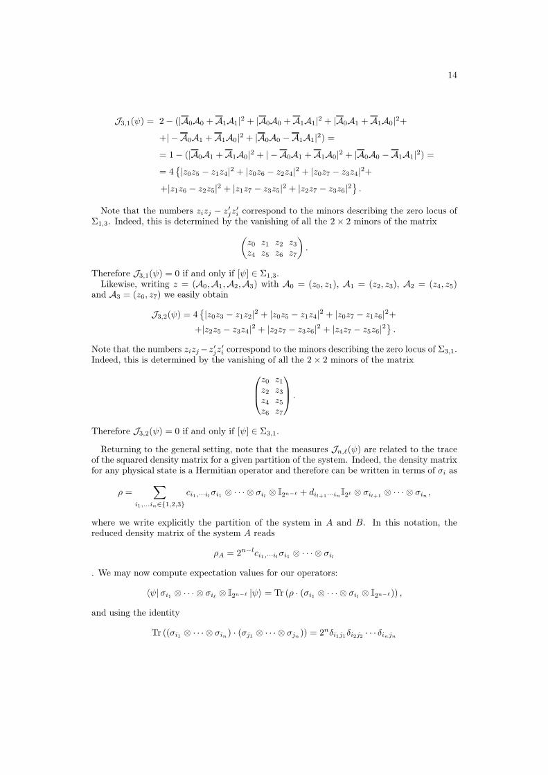
14

J3,1(ψ) = 2− (|A0A0 +A1A1|2 + |A0A0 +A1A1|2 + |A0A1 +A1A0|2++| − A0A1 +A1A0|2 + |A0A0 −A1A1|2) == 1− (|A0A1 +A1A0|2 + | − A0A1 +A1A0|2 + |A0A0 −A1A1|2) == 4

{

|z0z5 − z1z4|2 + |z0z6 − z2z4|2 + |z0z7 − z3z4|2++|z1z6 − z2z5|2 + |z1z7 − z3z5|2 + |z2z7 − z3z6|2

}

.

Note that the numbers zizj − z′jz′i correspond to the minors describing the zero locus of

Σ1,3. Indeed, this is determined by the vanishing of all the 2× 2 minors of the matrix

(

z0 z1 z2 z3z4 z5 z6 z7

)

.

Therefore J3,1(ψ) = 0 if and only if [ψ] ∈ Σ1,3.Likewise, writing z = (A0,A1,A2,A3) with A0 = (z0, z1), A1 = (z2, z3), A2 = (z4, z5)

and A3 = (z6, z7) we easily obtain

J3,2(ψ) = 4{

|z0z3 − z1z2|2 + |z0z5 − z1z4|2 + |z0z7 − z1z6|2++|z2z5 − z3z4|2 + |z2z7 − z3z6|2 + |z4z7 − z5z6|2

}

.

Note that the numbers zizj−z′jz′i correspond to the minors describing the zero locus of Σ3,1.Indeed, this is determined by the vanishing of all the 2× 2 minors of the matrix

z0 z1z2 z3z4 z5z6 z7

.

Therefore J3,2(ψ) = 0 if and only if [ψ] ∈ Σ3,1.

Returning to the general setting, note that the measures Jn,ℓ(ψ) are related to the traceof the squared density matrix for a given partition of the system. Indeed, the density matrixfor any physical state is a Hermitian operator and therefore can be written in terms of σi as

ρ =∑

i1,...in∈{1,2,3}ci1,···ilσi1 ⊗ · · · ⊗ σil ⊗ I2n−ℓ + dil+1···inI2ℓ ⊗ σil+1

⊗ · · · ⊗ σin ,

where we write explicitly the partition of the system in A and B. In this notation, thereduced density matrix of the system A reads

ρA = 2n−lci1,···ilσi1 ⊗ · · · ⊗ σil

. We may now compute expectation values for our operators:

〈ψ|σi1 ⊗ · · · ⊗ σiℓ ⊗ I2n−ℓ |ψ〉 = Tr (ρ · (σi1 ⊗ · · · ⊗ σil ⊗ I2n−ℓ)) ,

and using the identity

Tr ((σi1 ⊗ · · · ⊗ σin) · (σj1 ⊗ · · · ⊗ σjn)) = 2nδi1j1δi2j2 · · · δinjn

15

we obtain

ci1,···il = 2n 〈ψ|σi1 ⊗ · · · ⊗ σiℓ ⊗ I2n−ℓ |ψ〉 .

We now compute the trace of the squared density matrix:

TrAρ2A = 22(n−l)ci1,···ilcj1,···jlTr ((σi1 ⊗ · · · ⊗ σin) · (σj1 ⊗ · · · ⊗ σjn)) = 2l 〈ψ|σi1⊗· · ·⊗σiℓ⊗I2n−ℓ |ψ〉2

which leads to the identity

Jn,ℓ(ψ) = 2(

1− TrAρ2A

)

.

The main result of this section is the following:

Theorem IV.3. Let |ψ〉 be a pure n-particle state and let 1 ≤ ℓ ≤ n− 1. Then

Jn,ℓ(ψ) = 4∑

I

|MI |2,

where the sum runs over all 2 × 2 minors MI determining the zero locus of ΣNℓ,Nn−ℓ. In

particular,

Jn,ℓ(ψ) = 0 ⇐⇒ [ψ] ∈ ΣNℓ,Nn−ℓ.

Proof. Write (z0, · · · , zNn) = (A0, · · · ,ANℓ

), where

Aj = (zj(Nn−ℓ+1), · · · , zj(Nn−ℓ+1)+Nn−ℓ)

for j = 0, · · · , Nℓ, so that each Aj is tuple with Nn−ℓ + 1 components. With this notation,we have

Jn,ℓ(ψ) = 4

Nℓ−1∑

j=0

Nℓ∑

k>j

(||Aj ||2 · ||Ak||2 − |Aj · Ak|2).

Applying the Lagrange identity we obtain

Jn,ℓ(ψ) = 4

Nℓ−1∑

j=0

Nℓ∑

k>j

Nℓ−1∑

s=0

Nℓ∑

t>s

|Aj,s · Ak,t −Aj,t · Ak,s|2,

where Ai,j denotes the j-th component of the tuple Ai. It now suffices to note that thenumbers

Aj,sAk,t −Aj,tAk,s

correspond to the minors MI . Indeed, the zero locus of ΣNℓ,Nn−ℓis determined by the

vanishing of the 2× 2 minors of the matrix

A0,0 · · · A0,Nn−ℓ

......

ANℓ,0 · · · ANℓ,Nn−ℓ

.

16

V. PHYSICAL INTERPRETATION

Given an integer n ≥ 1, we fix an ordered basis of Nn = 2n − 1 linearly independentvectors of the Hilbert space of pure n-particle states of spin- 12

|i1 · · · in〉O1···On= |i1〉O1

⊗ · · · ⊗ |in〉On,

where O1, · · · ,On denote the different observers. We will omit the labels of the observers,but one should note that, in the following, the chosen basis always has the same fixed orderunless stated otherwise.

Definition V.1. Let 1 ≤ q ≤ n be an integer. An n-particle state |ψ〉 is said to be q-partiteif it can be written as

|ψ〉 = |ψ1〉 ⊗ · · · ⊗ |ψq〉 ,

where |ψi〉 are ni-particle states, with ni > 0 and n1 + · · ·+ nq = n.

1-partite states are called entangled, while n-partite states are called separable. Physically,separable states are those that are uncorrelated. A product state can thus be easily preparedin a local way: each observer Oi produces the state |ψi〉 and the measurement outcomes foreach observer do not depend on the outcomes for the other observers.

A basic observation is that a state is separable if and only if it lies in the generalized Segrevariety of Definition III.2 (see for instance [5]). Likewise, a state is q-partite if and only ifits corresponding projective point on PNn lies in a Segre variety of the form

ΣNm1 ,··· ,Nmq

withm1, · · · ,mq positive integers such thatm1+· · ·+mq = n. So q-partite states correspondgeometrically to the q-decomposable points of Definition III.4. Combining the results of theprevious two sections we have that an n-particle state |ψ〉 is q-partite if and only if there areq − 1 indices ℓ1, · · · , ℓq−1 with 1 ≤ ℓi ≤ n − 1 and ℓi 6= ℓj such that Jn,ℓi(ψ) = 0. Indeed,from Theorem III.6 we know that |ψ〉 is q-partite if and only if its corresponding point [ψ] inPNn lies in at least q − 1 different Segre varieties of the form ΣNℓ,Nn−ℓ

, with 1 ≤ ℓ ≤ n− 1.Moreover, from Theorem IV.3 we know that [ψ] ∈ ΣNℓ,Nn−ℓ

if and only if Jn,ℓ(ψ) = 0.Note that, a priori, given an n-particle state, one would have to take (n − 1)! measures

of bipartite type to completely determine its q-decomposability (namely, for each possiblebipartition, check further bipartitions recursively). The hypercube approach tells us that itsuffices to take (n−1) measures, corresponding to the operators {Jn,ℓ} in order to determinecompletely its q-decomposability.

In the remaining of the section, we study the behaviour of the observables Jn,ℓ in someparticular cases of interest. We first introduce the average observable acting on n-particlestates:

J (ψ) :=1

n− 1

n−1∑

ℓ=1

Jn,ℓ(ψ).

The two- and three- particle states discussed in Section II which are invariant under per-mutations of the Hilbert basis (|Sep〉, |EPS〉, |GHS〉, |W 〉) allow for natural generalizationsto the n-particle case. We study their entanglement measures.

Note first that the separable n-particle state

|Sepn〉 := |0 (n)· · · 0〉

17

corresponds to the point in PNn given by

[Sepn] = [1 : 0 : · · · : 0]and so one easily verifies that J (Sepn) = 0.

The Schrödinger n-particle state is a superposition of two maximally distinct states

|Sn〉 :=1√2

(

|0 (n)· · · 0〉+ |1 (n)· · · 1〉)

.

It generalizes the two-particle state |EPS〉 and the three-particle state |GHZ〉 and it corre-sponds to the point in PNn given by

[Sn] = [1 : 0 : · · · : 0 : 1].

One easily computes Jn,ℓ(Sn) = 1 for all 1 ≤ ℓ ≤ n and so J (Sn) = 1. For n > 3, itsnot clear that the Schrödinger state exhibits maximal entanglement [19]. This observationagrees with our measures for Jn,ℓ, as we will see below.

We now consider a generalization of the W state for three particles, to the case of n-particles. For each fixed integer 0 ≤ k ≤ n, these states are constructed by adding allpermutations of generators of the form

|1〉⊗ (k)· · · ⊗ |1〉 ⊗ |0〉⊗ (n−k)· · · ⊗ |0〉with k states |1〉 and n− k states |0〉, together with a global normalization constant. Theseare clearly invariant with respect to permutations of the basis. Denote such states by

|Dn,k〉 =(

n

k

)− 12 ∑

permut

|1〉⊗ (k)· · · ⊗ |1〉 ⊗ |0〉⊗ (n−k)· · · ⊗ |0〉 .

These are known as Dicke states [20]. Note that |Dn,0〉 = |Sepn〉 and |D3,1〉 = |W3〉. In thecase of four particles we have

|D4,1〉 = 1√4(|1000〉+ |0100〉+ |0010〉+ |0001〉) ,

|D4,2〉 = 1√6(|1100〉+ |1010〉+ |1001〉+ |0110〉+ |0101〉+ |0011〉) ,

|D4,3〉 = 1√4(|1110〉+ |1101〉+ |1011〉+ |0111〉) .

Their corresponding points in P15 are

|D4,1〉 = [0 : 1 : 1 : 0 : 1 : 0 : 0 : 0 : 1 : 0 : 0 : 0 : 0 : 0 : 0 : 0],

|D4,2〉 = [0 : 0 : 0 : 1 : 0 : 1 : 1 : 0 : 0 : 1 : 1 : 0 : 1 : 0 : 0 : 0],

|D4,3〉 = [0 : 0 : 0 : 0 : 0 : 0 : 0 : 1 : 0 : 0 : 0 : 1 : 0 : 1 : 1 : 0].

We obtain the following table for the observables J4,ℓ:

|D4,1〉 |D4,2〉 |D4,3〉

J4,134 1 3

4

J4,2 1 1 1

J4,334 1 3

4

J 56 1 5

6

18

Note J (D4,2) = 1 as is the case for the state |S4〉. For more than four particles we obtainvalues > 1 for the observables Jn,ℓ. For instance, in the five particle case, we have:

|D5,1〉 |D5,2〉 |D5,3〉 |D5,4〉

J5,11625

2425

2425

1625

J5,22425

2725

2725

2425

J5,32425

2725

2725

2425

J5,41625

2425

2425

1625

J 45

5150

5150

45

.

In particular, we see that

J (D5,2) = J (D5,3) > J (S5) = 1.

For higher particle states the same pattern repeats itself, with the middle states

|Dn,⌊n2 ⌋〉 = |Dn,⌈n

2 ⌉〉

always exhibiting the largest entanglement as well as symmetries of the tables in bothdirections.

We end this section with some notable examples in the four- and five-particle cases. Thestate

|HS〉 = 1√6

(

|1100〉+ |0011〉+ ω |1001〉+ ω |0110〉+ ω2 |1010〉+ ω2 |0101〉)

where ω = e2πi3 is a third root of unity, was conjectured to be maximally entangled by

Higuchi-Sudbery [19] and it actually gives a local maximum of the average two-particle vonNeumann entanglement entropy [21]. Another highly (though not maximally) entangledstate, found by Brown-Stepney-Sudbery-Braunstein [22], is given by

|BSSB4〉 =1

2(|0000〉+ |+〉 ⊗ |011〉+ |1101〉+ |−〉 ⊗ |110〉) ,

where |+〉 = 1√2(|0〉+ |1〉) and |−〉 = 1√

2(|0〉 − |1〉). Our measures agree with these facts, as

shown in the table below.

|S4〉 |D4,2〉 |BSSB4〉 |HS〉

J4,1 1 1 34 1

J4,2 1 1 54

43

J4,3 1 1 1 1

J 1 1 1 109

.

In [23], a related measure of entanglement is introduced, based on vector lengths and theangles between vectors of certain coefficient matrices. While this measure is strongly relatedto concurrence and hence to the observables J , their measure Eavg does not distinguish thestates |BSSB4〉 and |HS〉. In contrast, we do find that

1 = J (BSSB4) < J (HS).

19

In [22], a highly entangled five-particle state is described as

|BSSB〉5 =1

2(|000〉 ⊗ |Φ−〉+ |010〉 ⊗ |Ψ−〉+ |100〉 ⊗ |Φ+〉+ |111〉 ⊗ |Ψ+〉) ,

where |Ψ±〉 = |00〉 ± |11〉 and |Φ±〉 = |01〉 ± |10〉. Our measures give:

|S5〉 |D5,2〉 |BSSB5〉

J5,1 1 2425 1

J5,2 1 2725

32

J5,3 1 2725

54

J5,4 1 2425 1

J 1 5150

1916

In particular, we see that

1 = J (S5) < J (D5,2) < J (BSSB5).

VI. SUMMARY AND CONCLUSIONS

Within a purely geometric framework, we have described entanglement of n-particle statesin terms of a hypercube of bipartite-type Segre maps. For simplicity, in this paper we haverestricted to spin- 12 particles, but the geometric results generalize almost verbatim to thecase of qudits. The hypercube picture allows to identify separability (or more generally,q-decomposability) in terms of a depth factor within the hypercube: the deeper a state liesin the hypercube, the more separable.

We have defined a collection of operators which measure the properties of a state inthe above geometric set-up. Given an n-particle state and having fixed an ordered basisof the total Hilbert space, there are 2n−1 different decomposability possibilities, given bythe different ordered q-partitions, for 1 ≤ q ≤ n. A standard way to characterize thedecomposability of such a state would be to consider, for any possible bipartition, all of itspossible bipartitions in a recursive way. This gives a total of (n− 1)! measures to be taken.Our hypercube approach says that it suffices to take (n−1) measures, given by the operatorsJn,ℓ, with 1 ≤ ℓ ≤ n− 1. So as the complexity of the problem grows factorially, our solutionjust grows linearly on n.

The operators Jn,ℓ measure the different bipartitions of the system, corresponding geo-metrically with the last (n− 1) edges of the Segre hypercube. The expected value of theseoperators is related with the quantum Tsalis entropy (q = 2) of both parts of the state. Theconcrete values of ℓ for which Jn,ℓ vanishes shows precisely in what edge of the hypercubethe state belongs or, more physically, in which parts the state is separable.

To illustrate the physical interest of our approach, we have computed the value of theoperators Jn,ℓ for various entangled states considered in the literature. The motivation formany of them arises in quantum computing and are therefore classified from the quantumcontrol perspective. In all cases, the proposed observables give results consistent with theexpectations.

20

Appendix A: Proof of the Generalized Decomposability Theorem

This appendix is devoted to the proof of Theorem III.6 on geometric decomposability.Let us first consider the tripartite-type Segre embedding

fk1,k2,k3 : Pk1 × Pk2 × P

k3 → PN(k1,k2,k3),

where we recall that

N(k1, · · · , kn) := (k1 + 1) · · · (kn + 1)− 1.

The following lemma relates the Segre varieties associated to it.

Lemma A.1. Let k1, k2, k3 be positive integers. Then

Σk1,k2,k3 = Σk1,N(k2,k3) ∩ ΣN(k1,k2),k3.

Proof. It suffices to prove the inclusion Σk1,N(k2,k3) ∩ ΣN(k1,k2),k3⊆ Σk1,k2,k3 . Recall that

we have identities

fk1,k2,k3 = fk1,N(k2,k3) ◦ (I× fk2,k3) = fN(k1,k2),k3◦ (fk1,k2 × I).

Let a = [ai], b = [bj ] and c = [ck] be coordinates for Pk1 , Pk2 and Pk3 respectively. We will

also let x = [xij ] and y = [yjk] be coordinates for PN(k1,k2) and PN(k2,k3) respectively, and

z = [zijk] will denote coordinates for PN(k1,k2,k3).We have:

(fk1,k2 × I)(a, b, c) = (x, c), with xij := aibj.

(I× fk2,k3)(a, b, c) = (a, y), with yjk := bjck.

fN(k1,k2),k3(x, c) = (z), with zijk := xijck.

fk1,N(k2,k3)(a, y) = (z), with zijk := aiyjk.

Given a point z = (zijk) ∈ PN(k1,k2,k3), we claim the following:

1. z ∈ Σk1,N(k2,k3) if and only if all the 2× 2 minors of the matrix

z000 · · · z0k2k3

......

zk100 · · · zk1k2k3

vanish, so that zijk · zi′j′k′ = zi′jk · zij′k′ for all i 6= i′ and (j, k) 6= (j′, k′).

2. z ∈ ΣN(k1,k2),k3if and only if all the 2× 2 minors of the matrix

z000 · · · z00k3

......

zk1k20 · · · zk1k2k3

vanish, so that zijk · zi′j′k′ = zijk′ · zi′j′k for all (i, j) 6= (i′, j′) and k 6= k′.

21

3. z ∈ Σk1,k2,k3 if and only if z ∈ ΣN(k1,k2),k3, so that zijk = xij · ck, and x = (xij) ∈

Σk1,k2 . This last condition gives the vanishing of the 2× 2 minors of the matrix

x00 · · · x0k2

......

xk10 · · · xk1k2

.

Therefore we have xij · xi′j′ = xij′ · xi′j for all i 6= i′, j 6= j′. This gives identities

zijk · zi′j′k′ = xij · ck · xi′j′ · ck′ = xi′j · ck · xij′ · ck′ = zi′jk · zij′k′

for all i 6= i′, j 6= j′ and k 6= k′.

Claims (1) and (2) are straightforward, while (3) follows from the identity

Σk1,k2,k3 = Im(fN(k1,k2),k3◦ (fk1,k2 × I)).

Assume now that z ∈ Σk1,N(k2,k3) ∩ ΣN(k1,k2),k3. Then the equations in (1) and (2) are

satisfied, and moreover we may write zijk = xij · ck. To show that z ∈ Σk1,k2,k3 it onlyremains to prove that xij · xi′j′ = xij′ · xi′j for all i 6= i′ and j 6= j′. By (1) we have

zijk · zi′j′k′ = xij · ck · xi′j′ · ck′ = xi′j · ck · xij′ · ck′ = zi′jk · zij′k′

for all i 6= i′ and (j, k) 6= (j′, k′). Take k = k′ such that ck 6= 0. This gives

c2k · xij · xi′j′ = c2k · xi′j · xij′ for all i 6= i′ and j 6= j′.

Since c2k 6= 0, we obtain the desired identities.

In order to prove the Generalized Decomposability Theorem it will be useful to denotethe cubical decomposition of

P1× (n)· · · ×P

1 −→ PNn

by the (n− 1)-dimensional hypercube whose vertices are given by tuples v = (v1, · · · , vn−1)

where vi ∈ {0, 1}, with initial vertex v0 = (0, · · · , 0) representing P1× (n)· · · ×P

1 and finalvertex vf = (1, · · · , 1) representing PNn . We will call |v| := v1 + · · · + vn−1 the degree of a

vertex. All edges are of the form

(v1, · · · , vn−1)[j]−→ (w1, · · · , wn−1)

where vi = wi for all i 6= j and wj = vj + 1 = 1, so that |w| = |v| + 1. Such an edgerepresents a contraction of a product × at the position j via a Segre embedding.

Example A.2. For example, the cubical representation of f1,1,1 is

(00)

[2]

��

[1]// (10)

[2]

��

(01)[1]

// (11)

,

22

and the cubical representation of f1,1,1,1 is

(000)

[1]

��

[2]

##●

●

●

●

●

●

●

●

[3]// (001)

[1]

��

[2]

##●

●

●

●

●

●

●

●

(010)

[1]

��

[3]// (011)

[1]

��

(100)[3]

//

[2]

##●

●

●

●

●

●

●

●

(101)

[2]

##●

●

●

●

●

●

●

●

(110)[3]

// (111)

.

We will say that a point z ∈ PNn lives in a vertex v = (v1, · · · , vn−1) if it is in the imageof the map v → vf given by the composition of all edges [i] such that vi = 0. It follows thatz is q-decomposable if and only if it lives in some vertex v of degree |v| = n− q.

Lemma A.3. Let v 6= v′ be two vertices of the same degree in the (n − 1)-dimensional

hypercube. Then there is a unique 2-dimensional face of the form

w′

[j]

��

[i]// v′

[j]

��v

[i]// w

and if z lives in w, v and v′, then it also lives in w′.

Proof. Since |v| = |v′| and v 6= v′, there are i, j such that vi = 0, v′i = 1, vj = 1, v′j = 0, andvk = v′k for all k 6= i, j. Let w and w′ be the vertices whose components are given by

wk = max{vk, v′k} and w′k = min{vk, v′k}.

This gives the above commutative square. Assume now that z lives in w, v and v′. It sufficesto consider two cases:

Case j = i + 1. In this case, the above commutative square represents morphisms of theform

A× Pk1 × Pk2 × Pk3 ×B

IA×Ik1×fk2,k3

×IB

��

IA×fk1,k2×Ik3

×IB// A× PN(k1,k2) × Pk3 ×B

IA×fN(k1,k2),k3×IB

��

A× Pk1 × P

N(k2,k3) ×BIA×fk1,N(k2,k3)×IB

// A× PN(k1,k2,k3) ×B,

where A and B are products of projective spaces. Therefore we can apply Lemma A.1 toconclude that z lives in w′.

Case j < i + 1. In this case, the above commutative square represents morphisms of theform

A× Pk1 × P

k2 ×B × Pk3 × P

k4 × C

��

// A× PN(k1,k2) ×B × P

k3 × Pk4 × C

��

A× Pk1 × Pk2 ×B × PN(k3,k4) × C // A× PN(k1,k2) ×B × PN(k3,k4) × C

.

23

Since z lives in w we may decompose z = (zA, z12, zB, z34, zC). Since it lives in v, we havez12 ∈ ΣN(k1,k2) and since it lives in v′ we have z34 ∈ ΣN(k3,k4). It directly follows that zlives in w′.

Theorem A.4 (Generalized Decomposability). Let n ≥ 2 and 1 < q ≤ n be integers. Apoint z ∈ PNn is q-decomposable if and only if it is in at least q− 1 different Segre varieties

of the form ΣNℓ,Nn−ℓ, with 0 ≤ ℓ ≤ n.

Proof. Using the cubical representation introduced above, it suffices to show that if z livesin q−1 different vertices v1, · · · , vq−1 of degree |vi| = n−2, then z lives in a vertex of degree(n− q). By recursively applying Lemma A.3 we find that z lives in the vertex v∗ of degree(n − q) whose components are v∗j = mini{vij}. This implies that z is q-decomposable. Theconverse statement is trivial.

[1] V. Vedral, M. B. Plenio, M. A. Rippin, and P. L. Knight, Phys. Rev. Lett. 78, 2275 (1997).[2] O. Gühne and G. Tóth, PhysRep 474, 1 (2009).[3] R. Horodecki, P. Horodecki, M. Horodecki, and K. Horodecki, Rev. Mod. Phys. 81, 865 (2009).[4] M. B. Plenio and S. Virmani, Quant. Inf. Comput. 7, 1 (2007).[5] E. Ballico, A. Bernardi, I. Carusotto, S. Mazzucchi, and V. Moretti, eds., Quantum physics

and geometry, Lecture Notes of the Unione Matematica Italiana, Vol. 25 (Springer, Cham,2019) pp. vii+172.

[6] I. Bengtsson and K. Życzkowski, Geometry of quantum states (Cambridge University Press,Cambridge, 2017) pp. xv+619, An introduction to quantum entanglement.

[7] D. C. Brody and L. P. Hughston, J. Geom. Phys. 38, 19 (2001).[8] I. Bengtsson, J. Brännlund, and K. Życzkowski, Internat. J. Modern Phys. A 17, 4675 (2002).[9] H. Heydari and G. Björk, J. Phys. A 38, 3203 (2005).

[10] H. Heydari, J. Phys. A 39, 9839 (2006).[11] H. Heydari, Int. J. Quantum Inf. 9, 555 (2011).[12] J. Grabowski, M. Kuś, and G. Marmo, J. Phys. A 45, 105301, 17 (2012).[13] M. Sanz, D. Braak, E. Solano, and I. L. Egusquiza, Journal of Physics A: Mathematical and

Theoretical 50, 195303 (2017).[14] X. Hu and Z. Ye, Journal of Mathematical Physics 47, 023502 (2006).[15] C. Tsallis and E. Brigatti, Continuum Mechanics and Thermodynamics 16, 223 (2004).[16] A. Peres, Quantum theory: concepts and methods, Fundamental Theories of Physics, Vol. 57

(Kluwer Academic Publishers Group, Dordrecht, 1993) pp. xiv+446.[17] W. Dür, G. Vidal, and J. I. Cirac, Phys. Rev. A 62, 062314 (2000).[18] D. M. Greenberger, M. A. Horne, and A. Zeilinger, “Going beyond Bell’s theorem,”

in Bell’s Theorem, Quantum Theory and Conceptions of the Universe , edited by M. Kafatos(Springer Netherlands, Dordrecht, 1989) pp. 69–72.

[19] A. Higuchi and A. Sudbery, Physics Letters A 273, 213 (2000).[20] R. H. Dicke, Phys. Rev. 93, 99 (1954).[21] S. Brierley and A. Higuchi, Journal of Physics A: Mathematical and Theoretical 40, 8455 (2007).[22] I. D. K. Brown, S. Stepney, A. Sudbery, and S. L. Braunstein, Journal of Physics A: Mathe-

matical and General 38, 1119 (2005).[23] C. Zhao, G.-w. Yang, W. N. N. Hung, and X.-y. Li, Quantum Inf. Process. 14, 2861 (2015).