Demonstration of visualization techniques for the...
84
General rights Copyright and moral rights for the publications made accessible in the public portal are retained by the authors and/or other copyright owners and it is a condition of accessing publications that users recognise and abide by the legal requirements associated with these rights. • Users may download and print one copy of any publication from the public portal for the purpose of private study or research. • You may not further distribute the material or use it for any profit-making activity or commercial gain • You may freely distribute the URL identifying the publication in the public portal If you believe that this document breaches copyright please contact us providing details, and we will remove access to the work immediately and investigate your claim. Downloaded from orbit.dtu.dk on: Jun 24, 2018 Demonstration of visualization techniques for the control room engineer in 2030. ELECTRA Deliverable D8.1. WP8: Future Control Room Functionality Marinelli, Mattia; Heussen, Kai; Strasser, Thomas; Schwalbe , Roman; Merino-Fernández, Julia ; Riaño, Sandra; Prostejovsky, Alexander Maria; Pertl, Michael; Rezkalla, Michel Maher Naguib; Croker, Julian; Evenblij , Berend ; Catterson, Victoria ; Chen, Minjiang Publication date: 2017 Document Version Publisher's PDF, also known as Version of record Link back to DTU Orbit Citation (APA): Marinelli, M., Heussen, K., Strasser, T., Schwalbe , R., Merino-Fernández, J., Riaño, S., ... Chen, M. (2017). Demonstration of visualization techniques for the control room engineer in 2030.: ELECTRA Deliverable D8.1. WP8: Future Control Room Functionality.
Transcript of Demonstration of visualization techniques for the...
General rights Copyright and moral rights for the publications made accessible in the public portal are retained by the authors and/or other copyright owners and it is a condition of accessing publications that users recognise and abide by the legal requirements associated with these rights.
• Users may download and print one copy of any publication from the public portal for the purpose of private study or research. • You may not further distribute the material or use it for any profit-making activity or commercial gain • You may freely distribute the URL identifying the publication in the public portal
If you believe that this document breaches copyright please contact us providing details, and we will remove access to the work immediately and investigate your claim.
Downloaded from orbit.dtu.dk on: Jun 24, 2018
Demonstration of visualization techniques for the control room engineer in 2030.ELECTRA Deliverable D8.1. WP8: Future Control Room Functionality
Marinelli, Mattia; Heussen, Kai; Strasser, Thomas; Schwalbe , Roman; Merino-Fernández, Julia ; Riaño,Sandra; Prostejovsky, Alexander Maria; Pertl, Michael; Rezkalla, Michel Maher Naguib; Croker, Julian;Evenblij , Berend ; Catterson, Victoria ; Chen, Minjiang
Publication date:2017
Document VersionPublisher's PDF, also known as Version of record
Link back to DTU Orbit
Citation (APA):Marinelli, M., Heussen, K., Strasser, T., Schwalbe , R., Merino-Fernández, J., Riaño, S., ... Chen, M. (2017).Demonstration of visualization techniques for the control room engineer in 2030.: ELECTRA Deliverable D8.1.WP8: Future Control Room Functionality.

Project No. 609687
FP7-ENERGY-2013-IRP
WP 8
Future Control Room Functionality
Deliverable D8.1
Demonstration of visualization techniques for the
control room engineer in 2030
16/01/2017
ELECTRA
European Liaison on Electricity Committed
Towards long-term Research Activities for Smart
Grids

Project ID: 609687
16/01/2017 Page 2 of 83
ID&Title D8.1
Demonstration of visualization techniques for
the control room engineer in 2030
Number of pages: 83
Short description (Max. 50 words):
Deliverable 8.1 reports results on analytics and visualizations of real time flexibility in support
of voltage and frequency control in 2030+ power system. The investigation is carried out by
means of relevant control room scenarios in order to derive the appropriate analytics needed
for each specific network events.
Version Date Modification’s nature
V0.01 01/06/2016 First Draft
V0.02 30/11/2016 Revised Draft
V1.0 12/12/2016 Final Draft
V1.4 19/12/2016 The document is issued for Internal Review
V1.5 03/01/2017 Reviewed by TOQA
V2.0 16/01/2017 Released
Accessibility
PU, Public
PP, Restricted to other program participants (including the Commission Services)
RE, Restricted to other a group specified by the consortium (including the Commission
Services)
CO, Confidential, only for members of the consortium (including the Commission
Services)
If restricted, please specify here
the group:
Owner / Main responsible:
T8.2 Leader: Mattia Marinelli (DTU)
Reviewed by:
WP 8 Leader:
Technical Project Coordinator:
Project Coordinator:
Henrik Bindner (DTU)
Helfried Brunner (AIT)
Luciano Martini (RSE)
03/01/2017
Final Approval by:
ELECTRA Technical Committee
TOQA appointed Reviewer:
Helfried Brunner (AIT)
Andrei Morch (SINTEF) 03/01/2017
Project ID: 609687
16/01/2017 Page 3 of 83
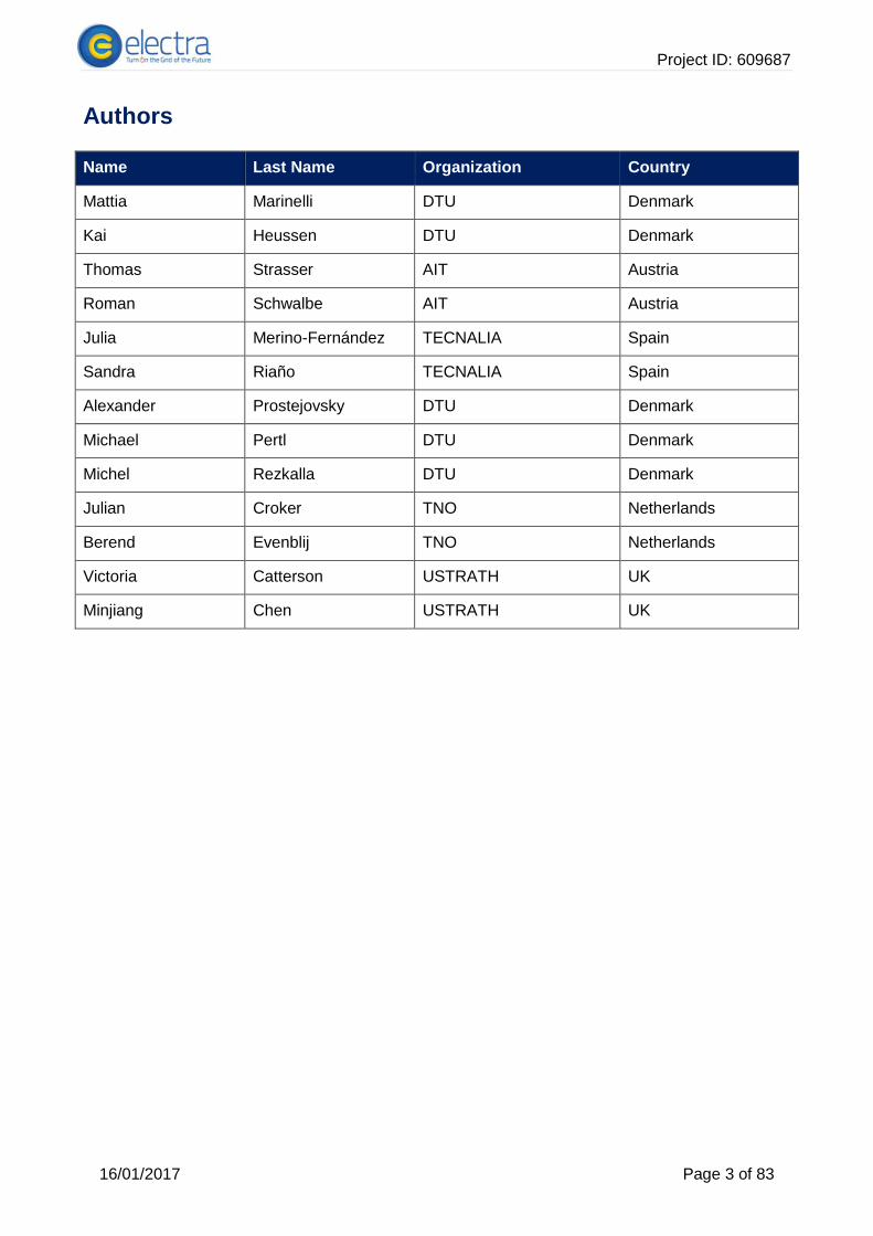
Authors
Name Last Name Organization Country
Mattia Marinelli DTU Denmark
Kai Heussen DTU Denmark
Thomas Strasser AIT Austria
Roman Schwalbe AIT Austria
Julia Merino-Fernández TECNALIA Spain
Sandra Riaño TECNALIA Spain
Alexander Prostejovsky DTU Denmark
Michael Pertl DTU Denmark
Michel Rezkalla DTU Denmark
Julian Croker TNO Netherlands
Berend Evenblij TNO Netherlands
Victoria Catterson USTRATH UK
Minjiang Chen USTRATH UK
Project ID: 609687
16/01/2017 Page 4 of 83
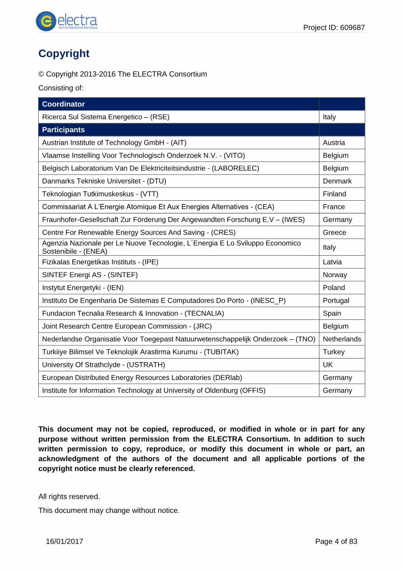
Copyright
© Copyright 2013-2016 The ELECTRA Consortium
Consisting of:
Coordinator
Ricerca Sul Sistema Energetico – (RSE) Italy
Participants
Austrian Institute of Technology GmbH - (AIT) Austria
Vlaamse Instelling Voor Technologisch Onderzoek N.V. - (VITO) Belgium
Belgisch Laboratorium Van De Elektriciteitsindustrie - (LABORELEC) Belgium
Danmarks Tekniske Universitet - (DTU) Denmark
Teknologian Tutkimuskeskus - (VTT) Finland
Commissariat A L’Energie Atomique Et Aux Energies Alternatives - (CEA) France
Fraunhofer-Gesellschaft Zur Förderung Der Angewandten Forschung E.V – (IWES) Germany
Centre For Renewable Energy Sources And Saving - (CRES) Greece
Agenzia Nazionale per Le Nuove Tecnologie, L´Energia E Lo Sviluppo Economico Sostenibile - (ENEA)
Italy
Fizikalas Energetikas Instituts - (IPE) Latvia
SINTEF Energi AS - (SINTEF) Norway
Instytut Energetyki - (IEN) Poland
Instituto De Engenharia De Sistemas E Computadores Do Porto - (INESC_P) Portugal
Fundacion Tecnalia Research & Innovation - (TECNALIA) Spain
Joint Research Centre European Commission - (JRC) Belgium
Nederlandse Organisatie Voor Toegepast Natuurwetenschappelijk Onderzoek – (TNO) Netherlands
Turkiiye Bilimsel Ve Teknolojik Arastirma Kurumu - (TUBITAK) Turkey
University Of Strathclyde - (USTRATH) UK
European Distributed Energy Resources Laboratories (DERlab) Germany
Institute for Information Technology at University of Oldenburg (OFFIS) Germany
This document may not be copied, reproduced, or modified in whole or in part for any
purpose without written permission from the ELECTRA Consortium. In addition to such
written permission to copy, reproduce, or modify this document in whole or part, an
acknowledgment of the authors of the document and all applicable portions of the
copyright notice must be clearly referenced.
All rights reserved.
This document may change without notice.
Project ID: 609687
16/01/2017 Page 5 of 83
Executive summary
IRP ELECTRA Task 8.2 focuses on analytics and visualization for the future control room of 2030+
in the Web-of-Cells context. The ELECTRA Web-of-Cells (WoC) concept emphasizes the
paradigm of solving local problems locally by operationally dividing the grid into cells, where local
operators are responsible for detecting and correcting real-time balancing and voltage deviations.
The present deliverable aims to derive new metrics and associated visualizations for future WoC
control rooms. Using an innovative scenario-based approach, situations are analysed for critical
information required to be available for operators by defining dedicated control room scenarios.
Several scenarios are based on the system-wide scenarios investigated in the task dealing with
observables for Pan-European control schemes [5], since they are related to the situations that
control room operators have to deal when system stability is at stake. Control loops invoked in the
control room scenario are taken from the high level use cases defined in the early stage of the
project [1], whilst detailed control variants are derived from the ones identified in the task analysing
the development of robust coordination functions for multiple controllers across different
boundaries [26]. The observables, that mean the processed information coming from the field and
used as inputs in the different control room scenarios, are either derived from the ones investigated
in the task dealing with observables for local control schemes or based on the ones defined in the
literature [2].
Chapter 1 provides an overview on the task methodology and connection with the aforementioned
project deliverables and the overall WP8 framework as well as recalling the main outcome of the
internal report 8.1 [7], where an overview of requirements for future control room is provided.
In Chapter 2 a set of relevant control room scenarios is identified. Three main drivers are identified
for defining the scenarios: scenarios that challenge traditional control schemes, scenarios that
caused major failures (i.e., blackouts) and scenarios that will happen in the future (not experienced
yet). A “vertical and horizontal” summary of the set of scenarios is outlined at the end of the
chapter.
Chapter 3 defines that control room flow of information for the selected pool of scenarios.
Sequence diagrams are defined in order to define information sent back and forth between field
and control room. Use cases invoked in specific control actions are identified as well as actions
that require manual intervention with the operator. The latter activity is bridging the activity with
T8.3 (development and demonstration of decision support).
Based on the discussions and interactions with different stakeholders (specifically DSOs and
TSOs), at the last CIRED 2016 workshop, different examples of visualization, connected to some
of the previously defined scenarios, are presented in Chapter 4.
Conclusions and final remarks are reported in Chapter 5.

Project ID: 609687
16/01/2017 Page 6 of 83
Terminologies
Acronyms
ELECTRA European Liaison On Electricity Committed Towards Long-Term Research Activity
AVR Automatic Voltage Regulator
BRC Balance Restoration Control
BRP Balance Responsible Party
BSC Balance Steering Control
BSP Balancing Service Provider
BSR Balance Steering Reserve
BUC Business Use Case
CIGRE International Council On Large Electric Systems
CIRED International Conference on Electricity Distribution
CSS Contributor to System Security
CTL Control Topology Level
CWA Cognitive Work Analysis (Methodology)
DER Distributed Energy Resources
DG Distributed Generation
DMS Distribution Management System
DN Distribution Network
DNO Distribution Network Operator
DOW Description Of Work
DR Demand Response
DRES Distributed Renewable Energy Sources
DSO Distribution System Operator
DSOpt Distribution System Optimizer
EDSO European Distribution System Operators
ENTSO-E European Network Of Transmission System Operators For Electricity
FACTS Flexible Alternating Current Transmission System
FCC Frequency Containment Control
FCR Frequency Containment Reserves
FRR Frequency Restoration Reserves
HV High Voltage
HVDC High Voltage Direct Current
ICT Information and Communication Technology
IDMS Integrated Distribution Management System
IFC Inertia Frequency Control

Project ID: 609687
16/01/2017 Page 7 of 83
IRP Integrated Research Programme
ISGT Innovative Smart Grid Technologies
LV Low Voltage
MV Medium Voltage
NEM Network Energy Management
NC Network Codes
NC- EB Network Code On Electricity Balancing
NC-CACM Network Code On Capacity Allocation And Congestion Management
NC-LFCR Network Code On Load Frequency Control And Reserves
NC-OPS Network Code On Operation Planning And Scheduling
NDZ Non Detection Zone
NPFC Network Power Frequency Characteristic
OP Operational Planning
OPF Optimal Power Flow
PAS Publicly Available Specification
PCC Point Of Common Coupling
PFC Primary Frequency Control
PMU Phasor Measurement Unit
PNDC Power Network Demonstration Center
PPVC Post Primary Voltage Control
PS Primary Substation
PV Photovoltaic
PVC Primary Voltage Control
PWM Pulse-width Modulation
RES Renewable Energy Sources
RMS Root Mean Square
ROCOF / RoCoF Rate Of Change Of Frequency
RR Replacement Reserves
SA Synchronous Area
SCADA Supervisory Control And Data Acquisition
SEI Software Engineering Institute
SFC Secondary Frequency Control
SGAM Smart Grid Architecture Model
SG-CG Smart Grid – Coordination Group
SGMM Smart Grid Maturity Model
SGS Speed Governing System
SOC State Of Charge
SUC System Use Cass
Project ID: 609687
16/01/2017 Page 8 of 83
TFC Tertiary Frequency Control
TN Transmission Network
TSO Transmission System Operator
TVC Tertiary Voltage Control
UC Use Case
VSC Voltage Source Converter
VSG Virtual Synchronous Generator
VSYNC Frequency support and stabilization by Virtual Synchronous Generators
WoC Web of Cells
WP Work Package
Abbreviations
D Deliverable M Milestone R Report

Project ID: 609687
16/01/2017 Page 9 of 83
Table of contents
1 Introduction ............................................................................................................................ 13
1.1 Future control room functionality ..................................................................................... 13
1.2 The ELECTRA approach ................................................................................................. 13
1.3 Outcome and recommendations for future control centers .............................................. 15
Distributed local controllers ...................................................................................... 16 1.3.1
ICT network status ................................................................................................... 16 1.3.2
System architecture and modularity ......................................................................... 16 1.3.3
Distributed resources flexibility ................................................................................. 17 1.3.4
System states and neighbour status ........................................................................ 17 1.3.5
1.4 Scope and methodology adopted for deriving analytics and associated visualizations .... 18
2 Control room scenarios identification ..................................................................................... 21
2.1 Chapter outline ................................................................................................................ 21
2.2 Restoration of transmission capacity during renewable energy production forecast error
(DTU_1) .......................................................................................................................... 21
2.3 Transient Stability Preventive Control (DTU_2) ............................................................... 22
2.4 Small signal stability - local and inter-area oscillations (DTU_3) ...................................... 23
2.5 Inter-cell loop flows (DTU_4) ........................................................................................... 24
2.6 Parameterization error detection of inverter-based DER (AIT_1) ..................................... 26
2.7 Normal operation until frequency collapse due to lack of system inertia (TNO_1) ........... 27
2.8 Unintentional islanding event in a single-tied cell (TEC_1) .............................................. 29
2.9 Proactive operation of the post-primary voltage control (TEC_2) ..................................... 30
2.10 Restoration of frequency after a single frequency excursion event (USTRATH_1) .......... 31
2.11 Restoration of frequency after two frequency excursion events within in the same cell
(USTRATH_2) ................................................................................................................. 32
2.12 Horizontal Requirements Assessment of Scenarios ........................................................ 33
Coverage ................................................................................................................. 33 2.12.1
Physical conditions and operational constraints of the scenarios ............................. 36 2.12.2
System response and Operator involvement ........................................................... 37 2.12.3
Visualization requirements ....................................................................................... 40 2.12.4
3 Control room concepts sequence diagrams ........................................................................... 42
3.1 Chapter outline ................................................................................................................ 42
3.2 Preventive transient stability (DTU_2) ............................................................................. 42
3.3 Inter cell loop flow (DTU_4) ............................................................................................. 43
3.4 Parameterization error detection of inverter-based DER (AIT_1) ..................................... 45

Project ID: 609687
16/01/2017 Page 10 of 83
3.5 Normal operation until frequency collapse due to lack of system inertia (TNO_1) ........... 45
3.6 Unintentional islanding event in a single-tied cell (TEC_1) .............................................. 47
3.7 Proactive operation of the post-primary voltage control (TEC_2) ..................................... 48
3.8 Single frequency deviation event (USTRATH_1) ............................................................. 49
3.9 Two simulation frequency events (USTRATH_2) ............................................................ 51
4 Visualization strategy approaches .......................................................................................... 53
4.1 Chapter outlines .............................................................................................................. 53
4.2 Foreword on visualization strategy and outcome of the interaction with stakeholders ...... 53
4.3 Visualization inertia allocation and exchange of inertia response power .......................... 55
4.4 Visualization clues for unintentional islanding detection and upcoming voltage control ... 58
4.5 Decentralised topology and power system state visualisation ......................................... 64
Dynamic topology assessment ................................................................................ 65 4.5.1
SYSLAB layout for market-based power matching algorithm ................................... 69 4.5.2
SYSLAB layout for individual and combined Use cases validation to be carried out in 4.5.3
ELECTRA lab-scale proof of concept activities ...................................................................... 72
5 Conclusions and future work .................................................................................................. 74
6 References ............................................................................................................................ 76
7 Disclaimer .............................................................................................................................. 79
A. Appendix ................................................................................................................................ 80
A.1 Scenario description tables ............................................................................................. 80

Project ID: 609687
16/01/2017 Page 11 of 83
List of figures and tables
Figure 2—1 Terms explaining inter-cell loop flows. Source: [5] ..................................................... 25
Figure 2—2 Real and ideal droop behavior of an inverter-based DER unit ................................... 27
Figure 2—3 Web-of-Cells scheme ................................................................................................ 29
Figure 2—4 Frequency management in Web-of-Cells ................................................................... 32
Figure 3—1 Sequence diagram for transient stability preventive control ....................................... 43
Figure 3—2 Sequence diagram for handling inter-cell loop flows. ................................................. 44
Figure 3—3 Sequence diagram for detecting parametrization errors in inverter-based DER. ........ 45
Figure 3—4 Sequence diagram for inertia coordination ................................................................ 46
Figure 3—5 Sequence diagram for unintentional islanding. .......................................................... 47
Figure 3—6 Sequence diagram for proactive voltage control. ....................................................... 48
Figure 3—7 Sequence diagram for single frequency event ........................................................... 50
Figure 3—8 Sequence diagram for two frequency events within the same cell ............................. 52
Figure 4—1 Example of TSO control room (National grid, UK) ...................................................... 53
Figure 4—2 Traffic light approach for visualizing the WoC ............................................................ 54
Figure 4—3 Architectural overview of inertia allocation ................................................................. 56
Figure 4—4 Synchronous area state visuals ................................................................................. 57
Figure 4—5 Cell state panel overview ........................................................................................... 57
Figure 4—6 CTL-3 view ................................................................................................................ 58
Figure 4—7 Visualization of CTL-3 in C-B ..................................................................................... 59
Figure 4—8 CTL-2 level in C-B ..................................................................................................... 59
Figure 4—9 CTL-3 level view in C-A ............................................................................................. 60
Figure 4—10 Loss of mains event at CTL-3 level .......................................................................... 61
Figure 4—11 Loss of mains event at CTL-2 level .......................................................................... 61
Figure 4—12 Resynchronization ................................................................................................... 62
Figure 4—13 Visualization of CTL-3 level regarding to scenario TEC-2 ........................................ 62
Figure 4—14 Visualization of CTL-2 level regarding to scenario TEC-2 ........................................ 63
Figure 4—15 Voltage deviation and short-term forecast visualization at CTL-2 level .................... 63
Figure 4—16 Visualization elements legend ................................................................................. 65
Figure 4—17 Modified PNDC test grid .......................................................................................... 65
Figure 4—18 Inter cell view of cell MV1 ........................................................................................ 66
Figure 4—19 Intra-cell view of cell MV2 as observed by the MV cell 1 agent ................................ 67
Figure 4—20 Local view of cell MV2 ............................................................................................. 68
Figure 4—21 Logical device assignments in (a) and data publishing directions in (b) ................... 68
Figure 4—22 Global topology view ............................................................................................... 69
Figure 4—23 SYSLAB grid as used for the PowerLabDK presentation. ........................................ 70
Figure 4—24 Inter-cell view on the SYSLAB simulation model...................................................... 71
Figure 4—25 Intra-cell view of cell CA_71X .................................................................................. 71
Figure 4—26 Local physical view of bus BA_715 .......................................................................... 72
Figure 4—27 Single diagram and simplified representation of different power components .......... 73
Table 1—1 Overview of Balance Control Use Cases and corresponding Control Aims ................. 14
Table 1—2 Overview of Voltage Control Use Cases and corresponding Control Aims .................. 15
Table 2—1 Scenario character ...................................................................................................... 34
Table 2—2 Network structure and configuration ........................................................................... 35
Table 2—3 Automatic control functions – CTL (Control topology level) vs UC (Use cases) ........... 35

Project ID: 609687
16/01/2017 Page 12 of 83
Table 2—4 Triggering events ........................................................................................................ 36
Table 2—5 Operators coordination ............................................................................................... 38
Table 2—6 Operator task analysis ................................................................................................ 39
Table 2—7 Overview of operational constraints ............................................................................ 40
Table 2—8 Visualization Requirements ........................................................................................ 41
Table 4—1 Information that should be displayed........................................................................... 55

Project ID: 609687
16/01/2017 Page 13 of 83
1 Introduction
1.1 Future control room functionality
The main objective of the related IRP ELECTRA activities in WP8 is to develop and demonstrate
the control room decision support that will be required for the real time operation of the 2030 power
systems, utilizing the visualization and control features being investigated in WP5 (increased
observability) and WP6 (control schemes for the use of flexibility) respectively to ensure that the
control room operator is provided with the optimal information of the state of the system and of the
possible control actions to enable taking preventive or corrective actions, in order to maintain or
return the system in safe state of operation.
With the increased flexibility within the power system, system-wide adoption of dynamic ratings,
pervasive control and automation, increasing market influence, etc., it is recognized that
significantly improved information and visualization is essential for future control rooms. It will
remain essential to have control engineers aware of system state and of potential threats, and
informed of the suitability of potential interventions to emerging critical situations. This work
package will demonstrate the means to achieving this and will be supported by direct interaction
with end users such as TSOs and DSOs on the development of measures/analytics/quantities that
provide the information needed for operators to quickly and easily assess the system state and
make safe/informed control actions to mitigate critical situations. It includes:
● Interaction with TSOs (Transmission System Operators), DSOs (Distribution System
Operators) and BRPs (Balancing Responsible Parties) to identify relevant
measures/analytics/quantities for preventive and corrective actions
● Develop prototype visualizations of the measures/analytics/quantities
● Development of decision support tools for control operators at TSO, DSO, BRPs control rooms
● Integration of the results with other systems being used by those congestion management,
market and trading systems.
1.2 The ELECTRA approach
On the whole, the approach adopted in ELECTRA to deal with power system control is based on a
power transmission and distribution system as a web of subsystems, called cells, which are
operated by Cell Operators (COs), namely entities similar to present TSOs. For control purposes, a
CO has to act on the inner resources of its own cell and can also cooperate with other COs, in
particular with the neighbouring cells COs, so that the whole power system, i.e. the whole Web-of-
Cells, is stable, secure and reliable [1].
A cell can be defined as a group of interconnected loads, concentrated generation plants and/or
distributed energy resources and storage units, all within well-defined grid boundaries
corresponding to a physical portion of the grid and to a confined geographical area; neighbouring
cells are connected by tie lines.
Based on operational security requirements a cell is in 'normal state' when in real-time operation:
It is able to follow the scheduled consumption/generation set-point so that the voltage,
frequency and power flows are within the operational security limits;
It is able to activate sufficient flexible ancillary resources (active and reactive power reserves).
A cell needs to aggregate sufficient flexible resources to manage the uncertainty (variability) due to
internal generation/load forecasting errors, but in case of need it can reach its balanced condition
Project ID: 609687
16/01/2017 Page 14 of 83
by interacting with neighbouring cells. A microgrid, instead, needs to aggregate sufficient resources
to potentially allow internal generation and load to balance without any external contributions, i.e.
to allow for islanded operation.
In order to keep a security operation of a cell, or a whole Web-of-Cells, in the normal state, two
main control types are needed:
● Balance Control, which includes all control loops (or control actions) that ensure, in real-time
operation, the power balance between generation and load;
● Voltage Control, which includes all control loops (or control actions) that ensure, in real-time
operation, that the voltage level at each node keeps within operational limits, in order to
transport the electricity energy from sending nodes (generation nodes) to receiving nodes
(consumption nodes) in a stable, secure and reliable way.
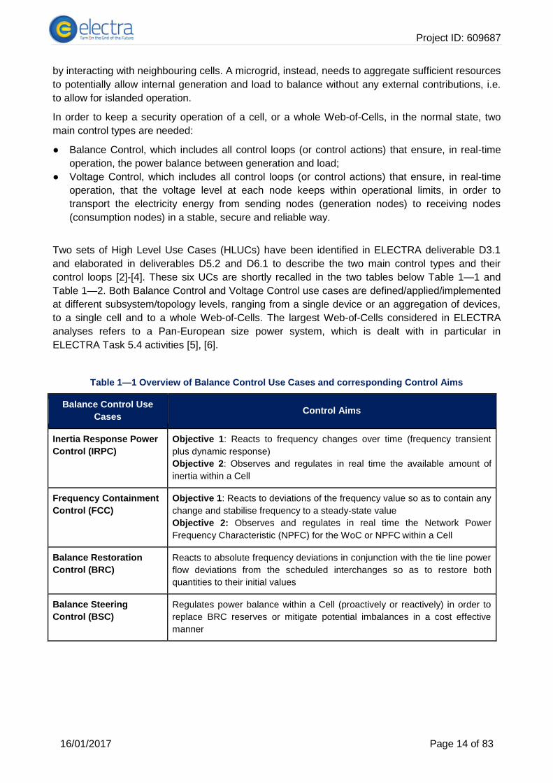
Two sets of High Level Use Cases (HLUCs) have been identified in ELECTRA deliverable D3.1
and elaborated in deliverables D5.2 and D6.1 to describe the two main control types and their
control loops [2]-[4]. These six UCs are shortly recalled in the two tables below Table 1—1 and
Table 1—2. Both Balance Control and Voltage Control use cases are defined/applied/implemented
at different subsystem/topology levels, ranging from a single device or an aggregation of devices,
to a single cell and to a whole Web-of-Cells. The largest Web-of-Cells considered in ELECTRA
analyses refers to a Pan-European size power system, which is dealt with in particular in
ELECTRA Task 5.4 activities [5], [6].
Table 1—1 Overview of Balance Control Use Cases and corresponding Control Aims
Balance Control Use
Cases Control Aims
Inertia Response Power
Control (IRPC)
Objective 1: Reacts to frequency changes over time (frequency transient
plus dynamic response)
Objective 2: Observes and regulates in real time the available amount of
inertia within a Cell
Frequency Containment
Control (FCC)
Objective 1: Reacts to deviations of the frequency value so as to contain any
change and stabilise frequency to a steady-state value
Objective 2: Observes and regulates in real time the Network Power
Frequency Characteristic (NPFC) for the WoC or NPFC within a Cell
Balance Restoration
Control (BRC)
Reacts to absolute frequency deviations in conjunction with the tie line power
flow deviations from the scheduled interchanges so as to restore both
quantities to their initial values
Balance Steering
Control (BSC)
Regulates power balance within a Cell (proactively or reactively) in order to
replace BRC reserves or mitigate potential imbalances in a cost effective
manner

Project ID: 609687
16/01/2017 Page 15 of 83
Table 1—2 Overview of Voltage Control Use Cases and corresponding Control Aims
Voltage Control Use
Cases Control Aims
Primary Voltage Control
(PVC)
Objective 1: Reacts in case of voltage deviations detected in any nodes of a
Cells as a consequence of a severe disturbance
Objective 2: observes, monitors and regulates the voltage levels deviations
in real-time in the grid nodes within the Cells
Post-Primary Voltage
Control (PPVC)
Objective 1: Restores the voltage levels in the grid nodes to the set-point
values within in a safe band. Simultaneously, it optimize the reactive power
flows in the system.
Objective 2: regulates the voltages in the nodes in case of generation-
demand imbalances
1.3 Outcome and recommendations for future control centers
The main goal of task T8.1 was to identify and define requirements to support data interpretation,
quantification of system threats and critical decision support [7]-[9].
The roles and activities in the future control centres will evolve with respect to the manual
switching, dispatching and restoration functions currently active. The control centre operators will
supervise on the power system and intervene - when necessary - thanks to the maturation and
wide scale deployment of flexible controls.
This report represents the starting point of WP8 activities with two objectives: the former is to
collect general requirements on future control centres emerging from the general trends in power
system operation and other European projects; the second is to consider the impact on future
control rooms of the ELECTRA proposed control solutions, developed in the other WPs.
The Use Cases developed within the European project “evolvDSO” highlighted the future roles and
services for the future DSOs. A focus on roles and services that evolvDSO envisages for the future
control rooms allowed the identification of a set of requirements [10].
The Web-of-Cells concept architecture proposed by ELECTRA has been analysed through the Use
Cases for voltage and frequency control developed within WP3 [1]. Hence, requirements for the
control centres, related to proposed control solutions have been identified. Even if this set of
requirements is related to the Web-of-Cells concept, some of them are aligned with general trends
and are common to other possible future architectures.
The qualitative analysis of the ELECTRA Use Cases by WP5 [2] allowed the alignment between
the observability needs and the technical challenges related to the proposed control schemes,
leading to the definition of requirements. Given that the ELECTRA architecture is still a novel idea,
the observability needs – and the related requirements - have been defined at high level.
The event occurred in the European electrical network on 4th November 2006 has been studied
and requirements have been extracted from lesson learnt [11]. The existing trends from vendors
were examined focusing on the experience in updating actual Distribution Management Systems
(DMS) and in understanding the current landscape. The need of analytics in innovative solutions,
to address smart grid challenges, emerges from the analysis of the existing software solutions
proposed by some vendors.

Project ID: 609687
16/01/2017 Page 16 of 83
Support in the definition of the final set of requirements for future control centres has been received
also from European DSOs, who answered to the questionnaire developed by T8.1 and described
the experiences they are having with smart grid demo projects.
Finally, the results have been summarized in a list of key requirements for future control centres
that are considered in WP8 activities. The requirements are categorized in the following
paragraphs.
Distributed local controllers 1.3.1
From all the sources analysed in this report it emerges that the future electrical systems will be
characterized by the presence of distributed local controls applied on parts of the distribution
network.
R1.1 The control room operator needs a topological view of the distribution system with a clear
indication of the network managed by each local controller.
R1.2 The status of local controller has to be displayed to the operator together with indicators of
normal/alert conditions and measures of achieved performance when the control is running.
ICT network status 1.3.2
Given the distributed nature of the control system and the strong interdependencies between the
electrical and the Information and Communication Technology (ICT) network in the future power
systems, control centres will have access to the status of the ICT network. The indicative status of
the ICT network will be provided by the ICT operators (which could be internal or external to the
network operator) on a need to know basis.
R2.1 The status of each local controller displayed to the operator includes indicators related to the
health status of the associated ICT infrastructure. These indicators will be based on real time data
from the ICT monitoring system provided by ICT operators.
R2.2 In case of alerts, errors or anomalous behaviour of one controller, the control room operator
must be able to switch off the controller and to operate manually. Moreover, he can access to more
detailed information (e.g. controller input/output data, detailed network status) useful to identify the
problem and to decide corrective actions.
Advanced control algorithms can implement adaptive behaviour that change control modes or
controller parameters depending on the status, availability and performance of the ICT
infrastructure.
R2.3 In case of controllers with different operational modes and automatic adaptive behaviour, the
control centre operators has to be informed on the currently active mode and be alerted on change
of control mechanisms.
System architecture and modularity 1.3.3
In a more dynamic evolution of the future energy scenarios, with increasing involvement of new
actors and resources in the control of the power system, it is important to enable fast and seamless
upgrading in control centres to follow the technological evolution, mainly ICT.
R3.1 Modular and open architecture is preferred for future control centres. The architecture will be
open to easily integrate new applications or visualization modules and to replace existing modules
with new ones without or minimizing the integration activities.
R3.2 Software modules will use standards interfaces, based on standard protocols and data
models, in order to achieve modularity and facilitate maintenance and update of control center
applications.

Project ID: 609687
16/01/2017 Page 17 of 83
Distributed resources flexibility 1.3.4
The direct involvement of flexible regulating resources in the network management will require the
control systems to interact with them (also via external actors, such as aggregators), exchanging
measures and set-points and control actions. The control center operators have to be aware of
forecast and actual behaviour of the resources, the available flexibility and their use.
R4.1 A set of observables for each controlled area/cell, including updated load and generation
forecasts, are available to the operator in order to foresee possible occurring of critical situations.
R4.2 At all times, the control center operator has access to the load and generation real time data
and to the available flexibility, in terms of active, reactive power and inertia, in each portion of the
network/cell.
System states and neighbour status 1.3.5
In a Web of Cell point of view each cell contains and stabilizes local voltage within secure limits
and contributes to contain and restore system frequency by maintaining operating schedules by
timely activation of local reserves. The control room operator has the role of monitoring the system
and its interconnections, to initiate control actions in response to critical events for secure and
stable operation. Cells (one or more) can be managed by a network operator.
R5.1 As a network operator may be responsible to manage more cells, adjacent or not, one control
centre has to provide to the control room operator all the necessary resources to monitor and
control many cells.
R5.2 The boundary of each cell has to be shown on the grid topology representation for the control
room operator.
R5.3 The state of each cell or sub-network can be displayed with different levels of detail.
R5.3.1 Synthetic indicators are used to inform the operator of normal condition or
constraints violation in the cell/sub-network.
R5.3.2 Moreover the operator can access detailed measurements of voltages and power
flows zooming in the cell.
R5.4 The operating state of each cell has to be monitored and displayed in real-time to ensure
continuous secure operation and the appropriate response to disturbances. Whereas many
systems are automatic, some responses may be manual.
R5.5 Any additional information at the boundary of each cell, needed to improve the coordination
with neighbouring cells regarding control actions that affect them as well, will be accessible to
control room operator.
R5.6 In addition to the cells in the area supervised by the control centre, the control rooms will
display also the summarized status of the neighbouring cells, under the responsibility of other
network operators, in order to improve the communication and the coordination among operators
of different areas of the power system.
From the analysis of major contingencies the following requirements may be added:
R6.1 In each control centre information related to the overall status of the synchronous area - in
particular the frequency measurements in neighbouring control areas - must be displayed to the
operator.
R6.2 The control area operator must to be able to monitor the activation of automatic mechanisms
(if exist) that can compromise the sharing of FCR – Frequency Containment Reserve – and FRR –
Frequency Restoration Reserve - of adjacent areas in order to manually intervene with
Project ID: 609687
16/01/2017 Page 18 of 83
countermeasures using own resources if necessary. In a Web of Cell architecture the same
requirement applies to each cell for Frequency Containment Control (FCC) and Balance
Restoration Control (BRC).
1.4 Scope and methodology adopted for deriving analytics and
associated visualizations
The objective of T8.2 is to develop appropriate analytics and associated visualisations that convey
system vulnerability and risk, measures of available flexibility, real-time headroom afforded by
dynamic ratings, and areas of congestion limiting market activity. Moreover, it aims to support the
oversight of real time operations, provide goal-driven interventions for control room operators with
appropriate decision support tools to support operations in a Web-of-Cells context.
Recommendations on how to deal with the potential escalation in complexity and uncertainty
driven by an increasingly distributed and renewable power system is investigated as well [12], [13].
Providing operators with actionable information instead of a “data tsunami” is becoming a critical
challenge for the distributed and more automated power system, therefore special attention is
given to provide information according to a need-to-know basis [14], [15].
The control room perspective entails that the ‘big picture’ of a web-of-cells coordinated power
system operation has to be taken into account. Whereas software/control solutions are designed
with separate objectives and stability problems in mind, in the cell operator perspective, an
overview of the overall system state has to be addressed. In view of the ELECTRA WoC concept,
the operator task is to supervise a highly automated power system operation and have the option
and capacity to intervene if necessary.
The operator support functions provided in the control room can be divided into three aspects:
● System monitoring: operator situational awareness; can you evaluate what is critical right
now?
● Supervisory control and interventions: offer input for operators to adjust system state
● Decision support: help operators identifying the right intervention.
Whereas the objectives for WoC (coordinated) control functions address decomposed sub-
problems of the power system, concerning future control room functionality, the task is to present a
common view of the automated power system state, including the state of both the physical
variables as well as the operation of control functions and objectives. Compared to the method for
definition of control functions in WP6, in WP8 the analytical context is the overall system operation
and operator point of view, rather than the context of a specific control objective. The design of
visualization and decision support systems for supervisory control of increasingly automated
systems is a challenge, as increasing automation does not necessarily reduce the cognitive effort
for operators, and in particular in critical situations, more automated systems have been reported
to cause a higher strain on an operator’s decision-making capacity [20], [21]. In order to define
detailed requirements for control room solutions, the designer thus has to understand what
constitutes relevant information to be presented to the operator [14].
To characterize these requirements for further technical analysis and design, the main outcome of
a further analysis is the identification and prioritization of this relevant information. To be able to
formulate this information, however, we need to provide a meaningful context of description and
analysis. A systematic approach to such requirements analysis for human machine interactions
has been developed as Cognitive Systems Engineering [16]. On this background, an analysis
methodology called “cognitive work analysis” (CWA) has been developed [18], [17]. CWA offers a
Project ID: 609687
16/01/2017 Page 19 of 83
stepwise methodology for systematically identifying and constructing a knowledge context in which
this relevant information can be described.
Given the speculative and anticipatory setting of the ELECTRA work, these requirements are hard
to identify directly from interviews with DSO operators, but can be derived and revisited from a
scenario analysis with domain experts instead.
The CWA analysis methodology [18] has been summarised as follows [24]:
“[…] the overall approach [consists] of five interrelated phases of modelling:
1. The work domain – purpose and structure of the system being controlled
2. Activity or control task analysis – what needs to be done in the work domain
3. Mental strategies – the mechanisms by which control tasks can be achieved
4. Social organisation – who carries out the work and how it is shared
5. Worker competencies – the set of constraints associated with the workers themselves.
In principle there are many specific modelling techniques that could serve for each of these
phases. […] The CWA approach therefore provides an interrelated set of methodologies
where these differing aspects of a system can be mapped, examined and analysed. For
example, CWA provides a means by which decision making within an environment can be
associated with system goals and cognitive skills.”
Adopting this methodology for the purpose of our analysis, the first step is therefore to describe
how the system (the work domain) ‘looks’ (presents itself) from the operator point of view: to
describe the operating objectives, power system and control functions at several levels of detail. In
common CWA practice, the Abstraction-Decomposition (Rasmussen’s abstraction hierarchy, [16])
space is applied for Step 1, and a hierarchically organized analysis of the operator’s decision-
making (Rasmussen’s decision-ladder [16]) is employed for Step 2.
A contribution of the ELECTRA project has been to demonstrate how the presently well-adopted
Use Case methodology can be employed to provide the type of information required for Step 1: by
formulating the required control structures and functions for the Web-of-Cells concept in both
abstract form (High-level use cases) and more detailed technical form (Detailed use cases) a clear
decomposition of the work domain has been formulated [26].
To address the Step 2 of the CWA methodology (control task analysis), critical operation scenarios
have been identified. These scenarios, called “Control Room Scenarios” and extensively described
in Chapter 2, are followed up by an analysis for visualization requirements in Section 2.12
Horizontal Requirements Assessment of Scenarios.
The elements identified in each scenario are listed below and can be related to CWA and
situational awareness (SA) contexts ([23], [25]):
1. control room scenario name;
2. network layout; initial conditions and schedule (domain context)
3. categorization of scenario (characterization of scenario assumptions)
4. involved operators and coordination among operators (social context)
5. triggering event (starting point of an event sequence; trigger in decision ladder)
6. relevant physical and operational constraints (interpretation and prioritization of system state;
information analysis / comprehension)
7. initially/automatically affected control loops (use cases; automatic response/automation)
8. Grid visualization (context representation/ information acquisition)

Project ID: 609687
16/01/2017 Page 20 of 83
9. operator 1st task - awareness of system change of state and operating state (SA - situational
awareness)
10. operator 2nd task - decision/action (Level 2 SA with decision & action)
11. operator 3rd task - optimization (Level 3 SA; operator cooperation with decision support
system)
12. relevant analytics (e.g. available control capacity from flexibility resources)
It can be observed that pragmatic simplifications have been performed in the formulation of this
method. These simplifications have been motivated from the perspective that a pragmatic analysis
that is approachable for the project participants will generate more relevant results than a rigorous
analytical approach that has the risk of alienating the participants. As Endsley, [19], reports, “the
problem of meaning [ought to] be tackled head on”: the chosen formulation of the SA and CWA
methodology for scenario analysis offered more significance for the project participants than a pure
approach.
This pragmatic approach has been further pursued in the following Chapter 3, where the control
tasks were analysed in terms of a sequence analysis, accounting both for required decisions and
analytics and the required information exchange.
This control scenario (control task) analysis is further deepened by a sequence analysis that
includes both operator and control system information and decision flows. Such an annotated
sequence diagram therefore addresses aspects of Steps 3 and 4 in the CWA methodology outlined
above. An analysis of “worker competencies” (CWA Step 5) has not been considered feasible to
address analytically at this stage.
However, the approach has been reflected on in Stakeholder consultations, acquiring feedback
from field experts, has been acquired, and first visualization prototypes have been developed. This
feedback and prototypes are reported in Chapter 4.

Project ID: 609687
16/01/2017 Page 21 of 83
2 Control room scenarios identification
2.1 Chapter outline
Following the state of the art analysis, in Chapter 2 a set of relevant control room scenarios is
identified. Three main drivers are identified for defining the scenarios: scenarios that challenge
traditional control schemes, scenarios that caused major failures (i.e., blackouts) and scenarios
that will happen in the future (not experienced yet).
Multiple scenarios are identified by all the ELECTRA partners at this stage even though some
overlapping may be present. A selection of scenarios is subsequently performed and the most
interesting scenarios are analysed further in Chapter 3 and Chapter 4.
The motivation and methodology of this approach has been introduced in the previous chapter. For
orientation, the elements identified in each scenario are:
1. control room scenario name (responsible in brackets);
2. network layout; initial conditions and schedule;
3. type of scenario (scenarios that challenge traditional control schemes; scenarios that caused
major failures; scenarios that will happen in the future (not experienced yet));
4. involved operators (specify if more than 1 operator is involved). Is coordination among
operators foreseen?
5. triggering event;
6. relevant physical and operational constraints (state variables and grid & flexibility capacity);
7. initially/automatically affected control loops (use cases);
8. grid visualization;
9. operator 1st task - awareness of system change of state and operating state;
10. operator 2nd task - decision/action;
11. operator 3rd task - optimization;
12. relevant analytics (available control capacity from flexibility resources).
A “horizontal” summary of the set of scenarios is provided at the end of this chapter in order to
derive a synthesis of control room information requirements. The set of scenarios investigated is
here listed:
A. Restoration of transmission capacity during renewable energy production forecast error
(DTU_1)
B. Transient Stability Preventive Control (DTU_2)
C. Small signal stability - local and inter-area oscillations (DTU_3)
D. Inter-cell loop flows (DTU_4)
E. Parameterization error detection of inverter-based DER (AIT_1)
F. Normal operation until frequency collapse due to lack of system inertia (TNO_1)
G. Unintentional islanding event in a single-tied cell (TEC_1)
H. Proactive operation of the post-primary voltage control (TEC_2)
I. Restoration of frequency after a single frequency excursion event (USTRATH_1)
2.2 Restoration of transmission capacity during renewable energy
production forecast error (DTU_1)
The first scenario has been derived by taking in account the events that initiated the European
system disturbance of the 4th of November 2006. As reported in [11], the system disturbance was

Project ID: 609687
16/01/2017 Page 22 of 83
mainly determined by a lack of coordination between neighbouring TSOs and poor information
exchange; however the massive power flow in that part of the grid was enhanced by stronger than
expected wind power production.
Starting from this event as source of inspiration, it has been decided to design the first control room
scenario, taking in consideration the fact that in the coming future, it will be more likely to face
events when the wind production may be larger than forecasted, threatening the transmission
capacity between two areas.
The control room scenario is triggered by a, larger than expected, production forecast that
consequently increases the power flow on a tie-line to a dangerous level for the system integrity.
The relevant physical and operational constraints are the tie-line flow and capacity as well as the
voltage level of the two ends of the line. The response from the control could be either automatic or
manual, depending on the specific network configuration. In any case it could either affect the
voltage level of the two terminals or invoking a re-dispatching action in the cell.
By controlling the voltage level, via available reactive power reserve, it is possible to marginally
increase the line capacity, obtaining in some cases the desired effect of effectively managing the
increased power flow. The post primary voltage control (PPVC) would be the use case invoked by
the control room.
By the balance steering control (BSC) use case it would be possible to re-dispatch some units
within the cell so that the overall cell balance is restored and the tie-line flow is kept within safe
limits. It has to be highlighted that the BSC could be applied to both a generating or consuming
unit, as long as the requested flexibility is achieved.
Concerning the grid visualization, it is important to have the possibility of observing the single line
diagram of the grid with relevant electric information and the reserve mix (both in term of
consumption and generation) of the cell.
In term of operator/control room actions, it is necessary to monitor the power flow through the
interested line and observe the voltage levels at both terminals. In that sense, it is important that
this specific information is exchanged between the two control rooms. It is also necessary to have
clear information on the protection settings at the two ends of the line, otherwise, one control room
operator may perform calculations taking in account a not realistic line capacity (this for instance
was one of the main misunderstanding that lead to the events of the 4th Nov 2006).
The second task of the operator (namely decision or action) is to activate one of the two use cases,
therefore either rescheduling some units (generation or consumption) or deploy reactive power
reserve in order to boost the voltage at the line terminals.
The third task instead focuses on monitoring the effectiveness of the controlling actions and
eventually updates other units’ schedules.
2.3 Transient Stability Preventive Control (DTU_2)
In future power system a high amount of distributed inverter-connected generation will be installed
and therefore the stability assessment for power systems will change radically [1]. Synchronous
generators will not dominate the power production anymore; instead, a significant part will be
covered from wind and PV power. Moreover, the energy mix of the generation will be increasingly
volatile over the course of a day, i.e. the basis for stability assessment has to be very
flexible/dynamic as the generation mix is changing with time.
Project ID: 609687
16/01/2017 Page 23 of 83
For analysis of the transient stability, the Pan European SRPS (single reference power system),
defined within ELECTRA [5], will be used. Transient stability is one of the key aspects of power
system stability since it describes the ability of keeping synchronism when subjected to large
disturbances, e.g. three-phase fault. Failing to maintain a sufficient level of transient stability in
terms of critical clearing time (CCT) could lead to widespread outages due to tripping of
generators, because synchronism is lost. Therefore, it is important to assess transient stability
online and set preventive actions if insufficient transient stability is determined, i.e. CCTs of certain
buses are lower than a user-specified limit (e.g. 200 ms). The most effective way to increase
transient stability is to dispatch the generators. The active power setpoint of critical generators has
to be reduced and the difference power shifted to uncritical generators. The needed dispatch to
achieve the desired transient stability limit is determined by the transient stability preventive control
decision support tool and the results are presented to the operator. The results include new active
power setpoints for the generators and the additional costs implied by the dispatch. Constraints,
such as generators’ capacity, maximal line flows and bus voltage limits are considered. As the
dispatch has to be carried out economically, the costs of generation are minimized while respecting
all technical constraints and the defined stability limit [27].
Since transient stability is assessed online and actions are set preventively, the BSC control loop is
affected as a new dispatch of generators is proposed to resolve the issues. The control room
operator has to verify and confirm the proposed dispatch or introduce additional constraints, such
as unavailability of generators to take over the dispatched power. In that case, a new dispatch is
proposed considering the additional constraints.
After applying the dispatch, the control room operator monitors the execution of actions and
verifies if the transient stability margins are re-established.
2.4 Small signal stability - local and inter-area oscillations (DTU_3)
Local and inter-area oscillations are inherent to power systems and are electro-mechanical
oscillations, whose stability is a prerequisite to secure system operation. Several blackouts have
been ascribed to those oscillations. Local modes normally have frequencies in the range from 0.7
to 2 Hz and inter-area modes have frequencies between 0.1 and 0.8Hz [28]. Local oscillations are
associated with one or a group of generators oscillating against the rest of the system. Inter-area
oscillations are associated with groups of generators that oscillate against each other.
The Pan-European SRPS which consists of several cells connected by HV transmission lines
builds the basis for the analysis. Within the WoC concept, cells can be tied over weak and strong
lines, therefore, both inter-area and local oscillations can occur.
Due to the paradigm shift from large centralized to small distributed generation the oscillation
behavior of power systems are changing. Moreover, at times of high renewable energy penetration
the number of synchronous generators which are supposed to damp these oscillations is reduced.
In that sense, these changing conditions challenge the existing traditional control schemes.
The scenario can involve one or two operators depending on the type of oscillations. In case of
local oscillations only one operator is involved while occurring inter-area oscillations can involve
two operators which generators are oscillating against each other.
Several triggering events are assumed for this scenario. It can be triggered by periodic variation of
the frequency or the active power on a transmission line exceeding a threshold. Moreover,
insufficient damping of a specific oscillation mode could be another trigger. Another trigger of
oscillations could be the change of generator setpoints or line switching.

Project ID: 609687
16/01/2017 Page 24 of 83
Several operational constraints have to be respected. The maximal amplitude of the periodic
variations must be kept within reasonable limits in order to ensure that equipment is not damaged.
A minimum damping of modes must be ensured in order to avoid increasing amplitude of those.
The rotor angle of generators must be kept at secure levels. Additional electrical constraints, such
as maximum line currents and active/reactive power limits of generators must be respected.
The control loops affected by the periodic variations are the IRPC, PVC, FCC and the BRC. The
IRPC, FCC and BRC are affected due to variations in frequency while the power system stabilisers
(PSS) are influencing the excitation system of synchronous machines and, therefore, the PVC in
order to damp oscillations. Moreover, static var compensators (SVC) which participate in voltage
regulation can be used to damp oscillations.
Continuously performed FFT (Fast Fourier Transform) of frequency and active power is used to
detect oscillations. The measurements might be provided by phasor measurement units (PMUs).
The FFT determines the oscillation modes, i.e. the frequency and damping of the modes. If
thresholds are exceeded, the control room operator gets issued a warning with information which
mode is poorly damped or which oscillation amplitude reached a critical limit. Perhaps even the
source of the problem can be identified which would facilitate to solve the problem.
As second task, the operator has to take a decision how to tackle the issue. A retuning of PSS or
other devices might resolve the issue. Moreover, a re-dispatch of generators or a topology change
by switching lines could be used to resolve the issue.
After applying the counteractions the control room operator has to observe the change in
frequency and damping of the modes and check if the problem is resolved.
2.5 Inter-cell loop flows (DTU_4)
The electricity market determines solutions for electric power flows based on the market prices and
subsequent bids of participants in the market. The balance steering control (BSC) determines flows
schedules based on the market solution, as these contracted flows do not necessarily follow
physical occurrences and the actual flows may differ in a meshed grid. Loop flows are therefore
defined as the deviation of the actual power flows from their scheduled values as described in [29]
and in [5].
Various reasons can cause loop flows, which may not be harmful per se but may lead to problems
when not considered. The two main factors are insufficient price signals, where market prices do
not reflect physical realities and constraints, as well as increasing energy imbalances due to
volatile renewable energy resources that are increasingly deployed in the grid.
Project ID: 609687
16/01/2017 Page 25 of 83
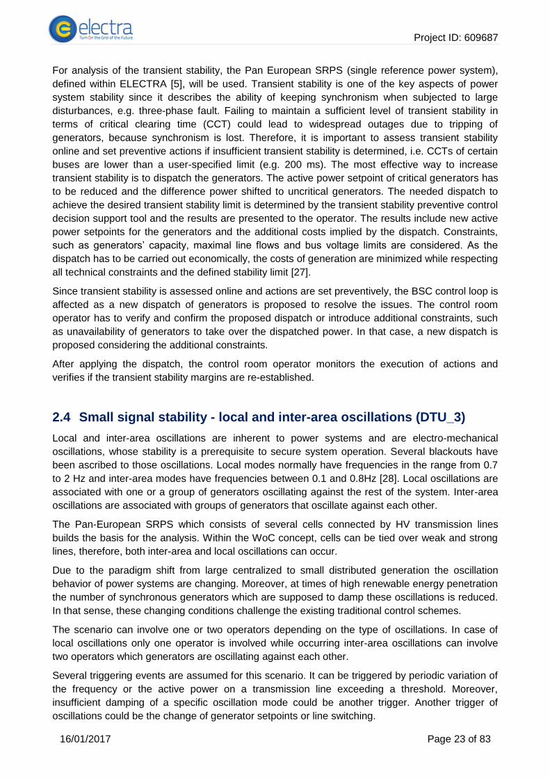
Figure 2—1 Terms explaining inter-cell loop flows. Source: [5]
Figure 2—1 illustrates various different flow situation in a meshed grid. The scheduled flow within
market participant (cell) A as part of the market solution is shown in a, whereas b shows the actual
emerging physical flow through neighbouring cells. The resulting unscheduled flow in c is the
difference between a and b. Loop flows are the parts of the scheduled flow that take alternative
paths as indicated in d. Inter-cell flows are essentially the same as within a cell, only that now the
scheduled power flow crosses cell borders via tie-lines as demonstrated in e between cells A and
D. The resulting inter-cell loop flow through cells B and C is given in e.
Problems related to loop flows are operational security, where unhandled flows can potentially lead
to blackouts, reduced economic and physical efficiency, and increased overall costs due to
contract violations, among others. For this reason, several mitigating means have been established
that allow the control of flows to a certain extent, such as phase-shifting transformers, series and
shunt compensators, etc. In addition, synchronous machines and HVDC links can be utilised to
alter loop flows.
ELECTRA is targeting in an automated control system that realises the best possible solution for
the scheduled flows under the given physical constraints. The balance steering control calculates a
physically feasible solution to the desired market operating points, which is then realised by the
BSC. Real-time monitoring of all production and consumption together with topological information
allows the control system to react immediately on changing conditions and steer the grid back to its
optimal operating point using available flexibility resources. Deviations from scheduled flows are
therefore minimized. The remaining permanent deviations should ideally be fed back into the
market and reflected in the price signals in order to mitigate unwanted flows after the next market
clearing.
From a control room operator’s point of view, significant deviations from the scheduled flows that
do not cease after balancing actions indicate problems in the automated control system. These
problems may have different causes, such as poor grid models the control is operating on,
corrupted live data streams within and from other cells, falsely reported operational states of
generators/breakers/etc., among many others that are outside of the normal operational state. It is
therefore the operator’s task to interpret unscheduled power flows for their potential causes and

Project ID: 609687
16/01/2017 Page 26 of 83
take appropriate countermeasures. Sticking to the mentioned examples, these measures could be
contacting other cell operators to update the grid models, checking the state of the IT network,
sending technicians on site to observe the actual state of devices, etc. In case of imminent tie-line
overloading, manual override of generators and loads near the affected line may be necessary to
relieve stress. In all cases, the decision support system should suggest possible causes and
solutions for the unscheduled loop flows to the operator, who evaluates them and (if applicable)
accepts or refuses the suggested mitigating action.
2.6 Parameterization error detection of inverter-based DER (AIT_1)
The future power system will be characterised by a high penetration of Distributed Energy
Resources (DER) powered by renewable sources (solar, wind, small-hydro). Latest trends in
research and industry show that inverter-based DER with advanced grid functions (e.g.,
voltage/frequency control support) are typically used to connect those devices to the power grid. In
addition, they can also be remotely controlled. Typically, such modern inverter-based DER
provides a lot of different parameters and remote control possibilities in order to optimally configure
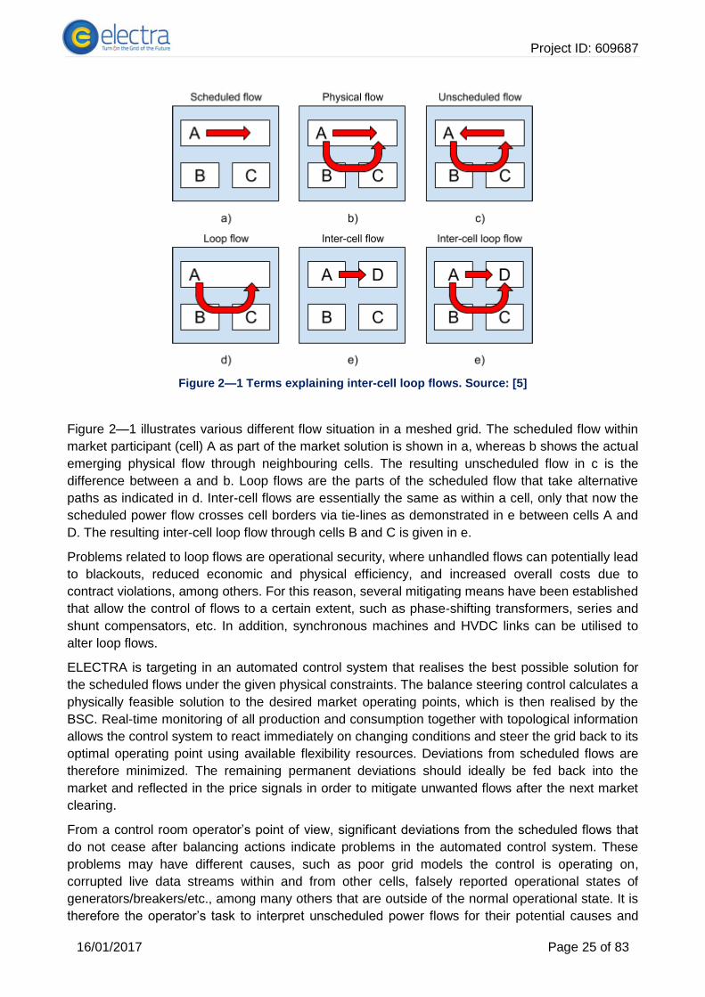
and operate them. There is a significant risk that those components are operated using wrong or
not optimal parameters from the grid operation point of view (see also Figure 2—2), especially
when a significant amount of generators in an ELECTRA Web-of-Cells is operated by inverter-
based DER.
Potential sources of faults are that the system integrator responsible for the installation of the
inverter-based DER uses wrong or not optimal parameters. Today, the grid operator typically
doesn’t get any direct information about the not optimal configuration of these components; only
the reaction can be usually observed (e.g., the violating a voltage threshold). This makes it usually
difficult to identify the source of the problem.
Therefore, this scenario deals with the analysis of control characteristics of inverter-based DER
units installed in context of the ELECTRA Web-of-Cell architecture. The idea is that the inverter
control parameters (characteristics) are monitored and analysed using the underlying
monitoring/ICT infrastructure. This can be carried out through a detailed analysis of measurements
indicating e.g., a voltage problem in the grid (i.e., trigger is the violation of a voltage threshold) by
the operator (e.g., visualized in GIS, voltage characteristic or voltage drop diagrams, scatter plots
Q(V), or in a single line diagram representation in a SCADA).
If a wrong or not optimal DER parameterization/configuration is detected, the operator has to be
informed (i.e., visualization in the control room), and if an automatic correction is not possible a
manual re-configuration might be necessary in order to solve this issue. Therefore, in general the
following three main actions can be performed remotely in order to re-configure the inverter-based
DER parameters:
● Reconfiguration of DER control parameter settings (e.g., droop curve)
● Output limitation of the DER (active and reactive power)
● Disconnection of the inverter-based DER unit from the power grid
Afterwards, the operator has to validate the impact of the performed action and may/may not
trigger further actions.
Project ID: 609687
16/01/2017 Page 27 of 83
Figure 2—2 Real and ideal droop behavior of an inverter-based DER unit
2.7 Normal operation until frequency collapse due to lack of system
inertia (TNO_1)
The grid is constantly subject to power variations. These may be due to small or large steps in load
or generation or, for instance, by tripping of tie-lines or transformers. These load steps are dealt in
most cases by increasing or decreasing power generated by synchronous machines. Because of
the inherent presence of inertial energy in the rotors of these generators, the ramp rate of the
frequency after a load step is limited. This gives the governor of the generator sufficient time to
adjust the power and secure a stable system frequency through a balance of supply and demand.
In the future grid, the synchronous generators will be gradually replaced by converter coupled
generation. During periods when converter based generation is meeting a significant proportion of
the demand, there could be insufficient inertia in the network from rotating synchronous machines,
as converters have no mechanically stored energy. This could result in increased RoCoF (Rate of
Change of Frequency) within the system and in severe cases the tripping of generators from the
operation of their protection relays.
One proposed solution, which has seen attention in literature, is to enable converters to imitate the
inertial behaviour of synchronous generators, through measurement of frequency fluctuations and
adjustment of the converter output. Additionally the activation of such features could be
coordinated to meet the dynamic stability requirements of a cell or group of cells.
This virtual inertia solution is based on the assumption that the converters do not react on short
notice to frequency deviations, resulting in the remaining synchronous generators having to take
care of all the power variations. When the converters have fast frequency droop response, the
frequency variations as well as the monitored RoCoF may be very small. This leads to a situation
where the instantaneous RoCoF, or 𝑑𝑓/𝑑𝑡, is high but at the same time the variation 𝛥𝑓 of the
frequency over a time window 𝛥𝑡is small, because 𝛥𝑓 is small.
Observe that the devices that monitor the RoCoF only register 𝛥𝑓/𝛥𝑡 and not instantaneous 𝑑𝑓/𝑑𝑡.
So fast frequency droop response could keep both the frequency variations small as well as keep
the registered RoCoF values below the triggering limit of the protection devices.

Project ID: 609687
16/01/2017 Page 28 of 83
The remainder of this paragraph leaves this option out of consideration and is on the assumption
that there is no fast frequency droop response active in the converters.
The frequency deviations from the rated value can be measured. This measurement starts with a
measurement of the frequency that should be sufficiently insusceptible to unbalanced and distorted
voltage waveforms. It takes some filtering, which introduces some time delay to generate a signal
that can be interpreted as the actual frequency. From this signal the rated value of the frequency
must be subtracted to obtain the frequency deviation. The same applies for the RoCoF. It is clear
that the shortest delay for the generation of the signal for the RoCoF is larger than the delay for the
generation of the signal for the frequency deviation. For both signals an RMS value can be
calculated based on a certain choice of a time window 𝛥𝑡 over which the mean value is taken. This
introduces another delay in signal of at least 1
2𝛥𝑡. For a meaningful result this 𝛥𝑡 should be at least
a few periods of the rated frequency. All of this makes the effectiveness of this control scenario
doubtful.
Two different methods are proposed to monitor the inertia within a synchronous area, a direct and
indirect method respectively. The direct method involves utilisation of SCADA (supervisory control
and data acquisition) communications to systems, where each inertial resource sends its status
and inertia information to the operator. The indirect method involves monitoring of the variations of
the system frequency (at a central node) to estimate the level of inertia.
To control the level of inertia in a synchronous area we also need to be able to deploy inertial
resources. From the swing equation, it can be derived that inertia reflects the proportionality
between frequency deviations and power deviations. For the indirect monitoring method knowledge
is needed about the specific power imbalance that induced the variations in the frequency to
estimate the total inertia. The question arises, what power flows should be measured to calculate
the total equivalent system inertia. For the direct monitoring method the inertia of each resource is
known and can summate to calculate the total system inertia. It is known that the inertia response
power, a certain generator is delivering, is dependent on the (electrical) distance to the location
where the originating power step occurs. This suggests that inertia, especially at the very
beginning the transient, can be regarded as local concept and cannot be directly attributed to a
grid. Additionally the inertia response also depends on the harmonic content of the wave shape of
the load step.
Within the ELECTRA control scheme development work is being done on this issue and the first
analyses hint at a more important role for fast frequency droop response.
An approach to circumvent to abovementioned problems is to collect the settings of the inertia
parameter of all the converters within the cell. Then an estimation of the biggest load step that can
occur within or nearby that cell is requested. If one assumes that all of this load step must be
handled by the aggregated inertia within the cell that is considered, a value of the desired inertia
can be calculated from the maximum allowable RoCoF. The maximum allowable RoCoF of a cell
can be obtained by considering the worst case generator, more specifically the settings of the
frequency protection relay.
Again on the assumption that within the cell the (electrical) distances (read: connecting
impedances of tie-lines and cables) is small, resulting in every supplier of inertia contributing in the
same measure, a request signal for the inertia setting for all the converters can be calculated
based on their reported available reserves. However, the question of whether (very) large amounts
of small units having inertia behaviour will lead to a stable system still remains to be seen.
Alternatively this could lead to oscillations that are similar to the inter-area oscillations that are
known from the classical grid, but now with much higher frequency and over much smaller
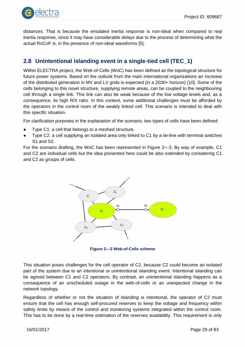
Project ID: 609687
16/01/2017 Page 29 of 83
distances. That is because the emulated inertia response is non-ideal when compared to real
inertia response, since it may have considerable delays due to the process of determining what the
actual RoCoF is, in the presence of non-ideal waveforms [5].
2.8 Unintentional islanding event in a single-tied cell (TEC_1)
Within ELECTRA project, the Web-of-Cells (WoC) has been defined as the topological structure for
future power systems. Based on the outlook from the main international organizations an increase
of the distributed generation in MV and LV grids is expected (in a 2030+ horizon) [10]. Some of the
cells belonging to this novel structure, supplying remote areas, can be coupled to the neighbouring
cell through a single link. This link can also be weak because of the low voltage levels and, as a
consequence, its high R/X ratio. In this context, some additional challenges must be afforded by
the operators in the control room of the weakly linked cell. This scenario is intended to deal with
this specific situation.
For clarification purposes in the explanation of the scenario, two types of cells have been defined:
● Type C1: a cell that belongs to a meshed structure.
● Type C2: a cell supplying an isolated area only linked to C1 by a tie-line with terminal switches
S1 and S2.
For the scenario drafting, the WoC has been represented in Figure 2—3. By way of example, C1
and C2 are individual cells but the idea presented here could be also extended by considering C1
and C2 as groups of cells.
Figure 2—3 Web-of-Cells scheme
This situation poses challenges for the cell operator of C2, because C2 could become an isolated
part of the system due to an intentional or unintentional islanding event. Intentional islanding can
be agreed between C1 and C2 operators. By contrast, an unintentional islanding happens as a
consequence of an unscheduled outage in the web-of-cells or an unexpected change in the
network topology.
Regardless of whether or not the situation of islanding is intentional, the operator of C2 must
ensure that the cell has enough self-procured reserves to keep the voltage and frequency within
safety limits by means of the control and monitoring systems integrated within the control room.
This has to be done by a real-time estimation of the reserves availability. This requirement is only

Project ID: 609687
16/01/2017 Page 30 of 83
applicable to type C2 cells because, from the cell definition, the self-sufficiency of resources is not
a necessary condition since the cell can rely on power imports/exports [1].
If faced with a not foreseen situation, S1 opens and S2 must disconnect for safety reasons.
Otherwise, an accidental reclosing of S1 could affect the equipment -or people- connected to C2.
Two operating conditions may be referred according to the situation preceding the S1 switch
opening.
● If there was a noticeable power exchange, the classical relay settings governing the operation
of S2 will enable the disconnection of S2 due to a change in the voltage, the frequency or the
rate-of-change of frequency (ROCOF).
● If the power exchange was not remarkable before the event, voltage and frequency excursions
could be so small to be undetectable by the classical relay settings. This situation would enter
inside the non-detection zone (NDZ) of the conventional methods, and therefore, S2 would not
open.
In the second case the future control room has to incorporate new measurements and visualization
techniques to allow the control and monitoring of additional variables as primary task of the
operator. These variables can be conventional, such as the power quality parameters or
impedances as well as more innovative such as the phase jumps registered from PMUs.
Nonetheless, these variables are directly depending on the connected elements and the
arrangement thereof inside the cell, which can also be reconfigurable. This obliges to the cell
operator to be exhaustive in the primary task of the real-time cell monitoring (i.e., SCADA). Its
secondary task will be the dynamic adjustment of the S2 switch settings and thresholds or the
remote controlling of the S2 openings and closings.
After the mains restoration, the S2 switch has to be closed again to bring back the system to the
primary operation snapshot. Prior to that, the controls of all the DER units connected to C2 must be
coordinated by its cell operator. The variation of the frequency and the angle in C2 requires the
operation over the aggregated P/f curve through the communication between the different DERs.
The connection/disconnection process of S2 is automatic, governed by an intelligent switch device.
However, the C2 cell operator has always the possibility to handle it manually. To ensure a safe C2
reconnection, critical measurements at both sides of the switch have to be monitored and
registered by the operator. Differences between voltage levels, phase angles and frequencies
before connecting C1 and C2 cells have to be small enough to avoid abrupt transients (oscillations)
in the reclosing stage. Also same voltage sequences must be checked. The whole process of
determining the adequacy for C2 reconnection is usually accomplished by the concurrent use of a
sequence detector, a PLL and a voltage comparator as part of the S2 static switch controls
2.9 Proactive operation of the post-primary voltage control (TEC_2)
In the analysis of future provision of ancillary services within ELECTRA, two control layers were
identified for the fulfilment of voltage control goals: primary and post-primary voltage (PPVC)
control. Since the primary voltage control will remain similar to the current practices -even new
devices will take action-, the post-primary voltage control will involve radical changes for the Web-
of-Cells control, monitoring and operational procedures.
This scenario focuses on the novel strategies to be accomplished by the cell operator in the control
room for the proactive operation of the PPVC. The PPVC, working in proactive mode, is intended
to reduce the number of triggers of the primary voltage controls by anticipating the voltage

Project ID: 609687
16/01/2017 Page 31 of 83
deviations in the nodes. Based on short-term forecasts and in 15-minute intervals analysis, the cell
operator compares the real-time voltage measurements with the expected voltages in the nodes.
This way it is possible to correct the voltage deviations in advance, avoiding unnecessary trips of
the PVC.
For the correct operation of the proactive PPVC the operator in the control room must have a
complete snapshot of:
● the measurements in the Web-of-Cells, including the voltages in the nodes, the tie-line power
flows, the available PPVC reserves etc.,
● the static information concerning the allowable voltage ranges in the nodes, the capacities of
the lines or the voltage safe bands for the nodes.
But it is also critical to have reliable forecasts (rooted on generation/load profiles) of the short-term
voltages in the nodes. In case of any bad measurement that could lead to the wrong operation or
even the windup of the control system, the PVC will act as the automatic backup mechanism.
Summarizing the tasks of the operator, the steps to follow in the operational procedure of the
proactive PPVC would be the following:
● Monitoring of the RMS voltage and the voltage deviation in the nodes
● Calculation of voltage short-term forecasts
● Estimation of the cell state for the following 15 minutes using real time measurements,
observables and short term forecasts
● Detection of unacceptable deviation of the voltages in any node with regards to the schedule
for the next 15 minutes
● Proactive activation of the PPVC reserves in accordance
2.10 Restoration of frequency after a single frequency excursion event
(USTRATH_1)
A critical incident which any network must be prepared to handle is that of a significant frequency
deviation event. Within the Web-of-Cells framework any event that causes a deviation in frequency
beyond the operational limits is managed by the following three services:
1. Frequency Containment Control (FCC): As the name suggests, the main responsibility of this
service is to stop the rise or fall of frequency and to contain it to a pre-defined value.
2. Balance Restoration Control (BRC): Once the frequency deviation has been contained, it is the
responsibility of BRC to restore the frequency back within the operational limits.
3. Balance Steering Control (BSC): Although the frequency has been restored by BRC, the
reserves that are utilized by BRC are fast acting and therefore may be expensive. These
reserves would need to be replaced for the remainder of the scheduled period. Therefore, it is
the responsibility of the BSC to replace the restoration reserves with the most economically
feasible resources.
As shown in Figure 2—4 there are two phases of frequency management within the Web-of-Cells
architecture: a procurement phase and real-time operation phase. Although the services described
earlier seem very similar to the services that are available to the operators today, it is the
distributed procurement and real-time delivery of these services necessary within the Web-of-Cells
paradigm that sets them apart. It is intended that the procurement of services is achieved by an
algorithm distributed amongst the cells within the network (hereafter referred to as the “inter-cell
algorithm”), which will fairly allocate resources to meet contingencies anticipated by each cell. The
implementation of this algorithm is out of the scope of this report.

Project ID: 609687
16/01/2017 Page 32 of 83
Figure 2—4 Frequency management in Web-of-Cells
Two main scenarios are considered here, which fall within the category of a frequency excursion
incident within the Web-of-Cells. The scenarios detail how the visualisations and decision support
might be provided to a cell operator under these circumstances. The first scenario is a single
frequency deviation event within a cell. The second one is two frequency deviation events
occurring within the same cell.
For the first scenario, the automatic frequency control scheme described above is envisaged to
automatically handle a single frequency disturbance event within a cell. That is, the deployment of
the procured reserves can fully restore the frequency within operational limits, and there is no
requirement for a human operator to take action. However, even if the system is automatically
resolving the single event, key information must still be relayed to the operator so that they are
kept well informed of what is happening within the network and how any particular incident is being
dealt with.
Decision support is also needed in this situation, to give the operator options for selection of
replacement reserves. The operator has a certain window of time in which to make their decision,
after which if no response has been received, the decision support automatically signals the cell
control to implement its own plan. In this way, the whole scenario is fully automated, but the
operator can observe and intervene if desired.
2.11 Restoration of frequency after two frequency excursion events
within in the same cell (USTRATH_2)
The second scenario describes two frequency events occurring within in the same cell. The second
frequency event occurs almost instantly after the first frequency deviation. Within this situation, it is
assumed that the procured restoration reserves are not sufficient to mitigate both events, meaning
that the BRC cannot restore the frequency to within normal operation levels purely by
implementing the plan from the procurement phase.
Therefore, all spare capacity from local devices and neighbouring cells should be determined. The
decision support system of the problem cell will prioritise the combination of reserves that mitigate
Project ID: 609687
16/01/2017 Page 33 of 83
this frequency event. Speed of response will be more important than cost, due to the emergency
situation. The scenario describes the communication between the problem cell and neighbours in
order to assess and procure emergency support.
In addition, the neighbouring cell experiences a challenge as they are being asked for larger
reserves than were previously promised to its neighbour. Therefore, the decision support of
neighbouring cell should indicate to the local operator how much spare capacity it can offer
immediately to the problem cell. If the cell has spare capacity that is uncommitted as reserves, it
should generally be offered to the problem cell. However, if the spare capacity of this cell has been
committed as BRC support to a third party, the choice of whether and how much support to offer
will depend on how soon the next planning phase starts.
That is, if the neighbour has unused reserves committed to a third party cell, and the next planning
phase begins in five minutes, the chance of the third party calling on those reserves will be
relatively small. Therefore, the neighbour may choose to offer some or all of the committed
reserves to the problem cell. But if the next planning phase begins in an hour, there is a higher
chance that another event will occur in the third party cell, and the committed reserves will be
required. If they have been consumed by the problem cell instead, the neighbour may be open to
penalties for failing to provide its contracted support to the third party. Therefore, a more cautious
offer of support may be given to the problem cell, including uncommitted reserves only.
As a result, the amount of BRC reserves offered to support to problem cell will vary based on
timing and the condition of the spare capacity (committed or uncommitted). Under the second
frequency deviation scenario, there is more of a requirement for human operators to participate in
the resolution of the situation, and the decision support options available to an operator should be
prioritised by taking these factors into account.
2.12 Horizontal Requirements Assessment of Scenarios
The scenarios have been compiled to create an overview of possible situations in future power
systems, which are viewed as controlled by the ELECTRA Web-of-Cells approach. The objective
of outlining these scenarios has been to identify specific requirements for visualization, analytics
and decision support. The contribution of this section is a cross-sectional analysis of the above
scenarios to first reflect the coverage of the investigated scenarios with respect to possible future
situations, network levels and topologies, and the WoC automatic control systems. Then the
scenarios characteristics are reflected to identify and summarize main requirements.
Coverage 2.12.1
Scenario character: Prior experience vs. future requirements
The WoC approach has been proposed to address the changes anticipated for future power
systems operation. Even though we place focus on these challenges, the approach also needs to
measure up against experience with today’s power system operation.
The scenarios are classified into three categories, summarized in Table 2—1:
1. Scenarios that caused major failures:
What was the cause of failure and why is it relevant for the future?
2. Scenarios that challenge traditional control schemes:
What is the new challenge, and why is it more relevant in the future?
3. Scenarios that will happen in the future (not experienced yet)):
What are the main drivers for these scenarios to appear?

Project ID: 609687
16/01/2017 Page 34 of 83
For the first two categories, the scenarios measure up the WoC qualities against existing system
operation: Major disturbances or blackouts point out where a lack of information or coordination is
present in current control room concepts, and enable an investigation on how the WoC concept will
respond to this existing challenge; the third category allows to outline the anticipated supervision
requirements.
Table 2—1 Scenario character
Scenario type # scenario
Explanation
Scenario that caused major failures
1 DTU_1: 4 Nov 2006 (European disturbance): trip of a tie-line causing a cascade of imbalance events that lead to eventual network separation, significant load shedding and partial blackout.
Scenarios that challenge traditional control schemes
2 TEC_1: current protection systems may be unable to detect the abnormal situation. Identification and integration of newer measurements such as THD ratios or phase jumps registered from PMUs for islanding detection TNO_1: low system inertia due to increased inverter coupled generation, increasing RoCoF, normal imbalances could result in a cascading failure resulting in frequency collapse; the challenge is the development of a new coordination scheme to ensure sufficient system inertia.
scenarios that can be expected happen in the future (not experienced yet)
8 TEC_2: high observability, improvements in the forecasting tools and numerical methods, which are oriented to anticipate grid problems, enhancing grid operation DTU_2: Increased situation awareness of control room operators’ about transient stability margins and support in decision making process to re-establish margins if they are too low. DTU_3: The generation mix and change of inertia in course of time affect the frequency and damping of the oscillation modes which could lead to undesired periodic variations. Moreover, SGs, equipped with a PSS, are switched off due to high RES production, i.e. fewer units are damping the oscillations. DTU_4: the increasing market complexity and higher level of interconnection at different voltage levels may cause consistent deviation between the market determined flows and physical flows. USTRATH_1: The frequency scenario with single deviation within the cell can be fully automated by a decision support system and the operator can observe and intervene if desired. USTRATH_2: Two frequency deviations events within the same cell will require more human operator to participate in the resolution of the situation, and decision support system will provide the options by taking time and the condition of the spare capacity (committed or uncommitted). AIT_1: The availability of powerful ICT infrastructure and remote control possibilities allows the improved monitoring of DER systems. TNO_1: The main driver for this scenario is the increasing penetration of inverter coupled generation, creating situations where synchronous generators with rotating inertia are displaced resulting in reduced network inertia.
Network structure and configuration
The defined scenarios cover all voltage levels from extra high voltage to low voltage grids. The
majority of network structures include meshed operation, but also radial operation is covered by
some scenarios. The defined network structures are mainly composed by interconnected AC grids
whereas DC overlay and interconnected variants are added on top because it is foreseen that the
expansion of point-to-point and multi-terminal DC grids will increase. DC grids will complement AC
grids primarily in the (extra) high voltage level and, therefore, DC components are only present in
the extra high voltage level. Moreover, another very important aspect concerning the development
of available inertia is covered by including the whole range from low to high inertia grid set-ups.
Several scenarios assume a high share of RES and analyse the impact of those from different
perspectives, such as restoration of transmission capacity during RES generation forecast error
and reduced synchronous inertia due to high RES generation. Loop flows which exist only in

Project ID: 609687
16/01/2017 Page 35 of 83
meshed grids are expected also to affect distribution grids in the future as there is a tendency to
also mesh them. Relevant properties of network layout for the scenario to be applicable: Voltage
level (HV, MV, LV), meshed or radial, complexity of the studied network (depth of model, number
of units). Scenarios can be applicable to only a subset of the feasible operating states of a given
configuration. The overview is reported in Table 2—2.
Table 2—2 Network structure and configuration
Voltage level (IEC 60038)
Meshed operation
Radial operation
Tie-line AC AC+DC Low inertia
High inertia
EHV (>230 kV)
DTU_1; DTU_2; DTU_3 DTU_4; AIT_1
AIT_1 DTU_1 DTU_1; AIT_1 DTU_1; DTU_2 DTU_3 DTU_4
DTU_2 DTU_3 TNO_1
DTU_2 DTU_3
HV (35 to 230 kV)
USTRATH_1 USTRATH_2 TEC_2; AIT_1
TEC_2; AIT_1 TEC_1; USTRATH_1 USTRATH_2
USTRATH_1; USTRATH_2; AIT_1
TEC_2 TEC_2
MV (1 to 35 kV)
USTRATH_1 USTRATH_2 TEC_2; AIT_1
TEC_2; AIT_1 TEC_1; USTRATH_1 USTRATH_2
USTRATH_1; USTRATH_2; AIT_1
TEC_2 TEC_2
LV (<1 kV)
TEC_2; AIT_1 TEC_2; AIT_1 TEC_1 AIT_1 TEC_2 TEC_2
Coverage of ELECTRA WoC automatic control functions
Table 2—3 summarizes to what extent the WoC control functions are reflected in the scenarios. As
outlined in ELECTRA D6.1, each control function can be operating at separate levels (on device –
CTL-0, on aggregates of devices - CTL-1, at cell-level CTL-2, and across several cells, CTL-3).
The control functions can be related to the scenario in several ways: they may be alleviating an
otherwise critical situation, they may be worsening the overall system response, or they may offer
the functions for an operator resolve an issue in the grid.
Table 2—3 Automatic control functions – CTL (Control topology level) vs UC (Use cases)
WoC control function
Control Topology Level
IRPC FCC BRC BSC PVC PPVC
CTL-0 DTU_2, DTU_4, TNO_1,
TEC_1 TEC_1, DTU_3, DTU_4
TEC_1, DTU_3, AIT_1, TEC_1, TEC_2
TEC_1,
CTL-1 TEC_1 DTU_3, DTU_4, USTRATH_1, USTRATH_2 TEC_1
TEC_1 TEC_1, TEC_2 DTU_3, AIT_1
TEC_1,
CTL-2 DTU_1, TNO_1
TEC_1, USTRATH_1
DTU_3, TEC_1, USTRATH_1, USTRATH_2,
TEC_1, USTRATH_1, USTRATH_2
TEC_1, TEC_2
TEC_1
CTL-3 DTU_1, TNO_1
TEC_1 TEC_1 TEC_1 TEC_1 TEC_1

Project ID: 609687
16/01/2017 Page 36 of 83
Physical conditions and operational constraints of the scenarios 2.12.2
An understanding of the physical conditions of a disturbance scenario is the foundation of the
scenario analysis. The logic is that a triggering event causes a physical phenomenon to occur,
which can be explained in terms of variation and violation of different operating constraints.
Operating constraints can be of physical nature, but also due to technical and market limits and
agreements.
Triggering event(s)
Conventional triggers, such as tripping of lines, transformers or generation units are initiating some
of the scenarios. Only one scenario analyses the system behavior to electrical faults which is in
this case a three-phase short-circuit. Other scenarios are triggered by newly introduced issues,
such as power flow deviations due to RES forecast error or critically low rotational inertia due to
high penetration of RES.
Triggers, such as violation of maximal line flows or voltage violations can be derived more
straightforwardly, e.g. line rating. However, the derivation of limits for the minimum available inertia
cannot be easily done as it is a grid-wide aspect, which needs a large variety of considerations
which affect the frequency control in power systems. Therefore, analysis has to be carried out to
understand the frequency dynamics in future power systems with high share of converter-based
units and how virtual inertia can contribute to improve the situation.
Most of the scenarios require a single trigger, in most cases a tripping of equipment. Some
scenarios require several subsequent triggers to occur as illustrated Table 2—4.
Table 2—4 Triggering events
Primary trigger 2nd trigger
Tripping of equipment Line trip (DTU_1), Line trip, Trafo trip (DTU_2) Loss of mains (TEC_1) Loss of generation (USTRATH_1,2) Time-based automatic trigger (TEC_2)
Electrical faults (DTU_2) Three-phase SC
Violation of operational limits Exceeded tie-line flow (DTU_4) Voltage violation (AIT_1)
Exciter (field) saturation (DTU_1)
Deviation of real vs. forecasted generation and demand
RES generation deviation (TNO_1) Generator dispatch deviation (DTU_3)
Insufficient rotating synchronous generators
Change in total system inertia (TNO_1) Change is worst case system imbalance (TNO_1)
Change in max allowable RoCoF for frequency stability
Analysis of operational constraints
The relevant constraints can be divided into three main categories where some are overlapping:
a) node constraints which include voltage limits, generator capacity, power flexibilities
Project ID: 609687
16/01/2017 Page 37 of 83
b) branch constraints which include maximum line flow and
c) global/area-wide constraints, which include network frequency, available reserves,
flexibility of a certain area, available inertia.
The identified constraints and their categorization are further listed in the Section on Visualization
Requirements, below.
An analysis of the physical and operational constraints and their effects in the scenarios yields a
number of additional requirements to be noted in the development of visualization, analytics and
decision support methods:
R-N-1 Stochastic influence of RES on tie-line flows causes uncertain deviations from scheduled
exchange which must be considered in the planning of secure exchange schedules (applies to AC-
tie lines, with consideration of special cases of radial and meshed operation).
R-N-2 A high share of converter-based generation reduces rotational synchronous inertia, which
makes it necessary to monitor overall available inertia (applies to synchronous region).
R-N-3 Physical power flows are not governed by cell- and market- defined (conceptual) system
boundaries, which means that exchanges across such abstract system boundaries will mismatch
the physical power flow (applies to cells interconnected by multiple tie-lines and with meshed
structure); physical network models are therefore required to evaluate security of planned
exchange schedules.
R-N-4 Coordinated operation of point-to-point and multi-terminal DC grids to support and increase
stability of AC grids.
System response and Operator involvement 2.12.3
Operating constraints are monitored manually or by automatic devices. An automatic response of
the WoC control functions should generate an overall more stable system behaviour. However,
technical control functions also extend the range of variables to be monitored by an operator, and it
has been found elsewhere that increased automation can be detrimental to situation awareness
[20]-[23]. The information provided in a visualization to support operator situational awareness
should then include both all relevant operational constraints as well as the operating state of WoC
control functions in principle, but the summary provided here should be considered as input for the
future consideration of testing scenarios and not as final requirements.
Automatic Response of ELECTRA WoC control functions
The WoC control functions related to the scenarios are listed in Table 1—1 and Table 2—3;
however, their involvement can have several roles. Control functions can be (a) affected initially,
which means that the monitoring of an automatic response will be required; there can be a (b)
secondary response of the automation function which may disturb the system state further; finally,
(c) the control function may offer a means to the operator for improving the operating state. This
involvement is different for each scenario. In general, it can be summarized that the following
different aspects of a control function need to be available to an operator:
1. Is the control function operational? (operational / fault condition)
2. How many resources are currently in use and allocated by the control function (reserve
status)?
a. How many are in use and how do these affect the physical network conditions?
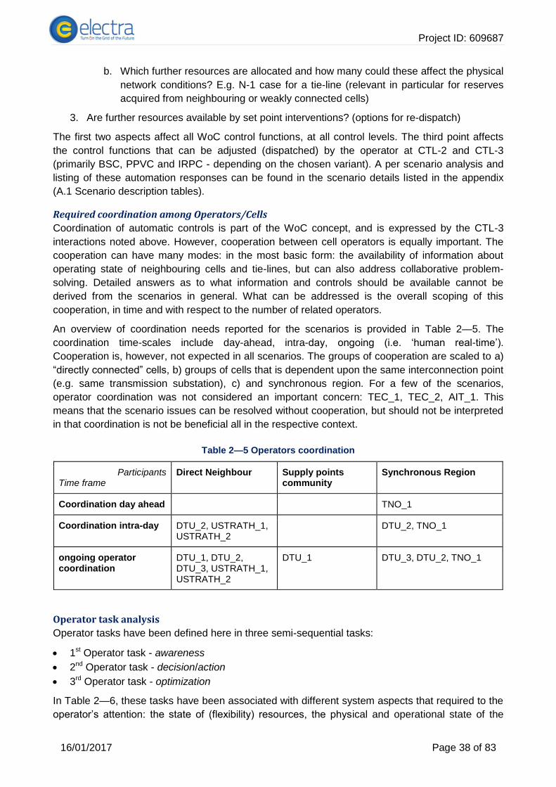
Project ID: 609687
16/01/2017 Page 38 of 83
b. Which further resources are allocated and how many could these affect the physical
network conditions? E.g. N-1 case for a tie-line (relevant in particular for reserves
acquired from neighbouring or weakly connected cells)
3. Are further resources available by set point interventions? (options for re-dispatch)
The first two aspects affect all WoC control functions, at all control levels. The third point affects
the control functions that can be adjusted (dispatched) by the operator at CTL-2 and CTL-3
(primarily BSC, PPVC and IRPC - depending on the chosen variant). A per scenario analysis and
listing of these automation responses can be found in the scenario details listed in the appendix
(A.1 Scenario description tables).
Required coordination among Operators/Cells
Coordination of automatic controls is part of the WoC concept, and is expressed by the CTL-3
interactions noted above. However, cooperation between cell operators is equally important. The
cooperation can have many modes: in the most basic form: the availability of information about
operating state of neighbouring cells and tie-lines, but can also address collaborative problem-
solving. Detailed answers as to what information and controls should be available cannot be
derived from the scenarios in general. What can be addressed is the overall scoping of this
cooperation, in time and with respect to the number of related operators.
An overview of coordination needs reported for the scenarios is provided in Table 2—5. The
coordination time-scales include day-ahead, intra-day, ongoing (i.e. ‘human real-time’).
Cooperation is, however, not expected in all scenarios. The groups of cooperation are scaled to a)
“directly connected” cells, b) groups of cells that is dependent upon the same interconnection point
(e.g. same transmission substation), c) and synchronous region. For a few of the scenarios,
operator coordination was not considered an important concern: TEC_1, TEC_2, AIT_1. This
means that the scenario issues can be resolved without cooperation, but should not be interpreted
in that coordination is not be beneficial all in the respective context.
Table 2—5 Operators coordination
Participants Time frame
Direct Neighbour Supply points community
Synchronous Region
Coordination day ahead TNO_1
Coordination intra-day DTU_2, USTRATH_1, USTRATH_2
DTU_2, TNO_1
ongoing operator coordination
DTU_1, DTU_2, DTU_3, USTRATH_1, USTRATH_2
DTU_1 DTU_3, DTU_2, TNO_1
Operator task analysis
Operator tasks have been defined here in three semi-sequential tasks:
1st Operator task - awareness
2nd Operator task - decision/action
3rd Operator task - optimization
In Table 2—6, these tasks have been associated with different system aspects that required to the
operator’s attention: the state of (flexibility) resources, the physical and operational state of the

Project ID: 609687
16/01/2017 Page 39 of 83
electrical network, and finally, stability considerations which relate to abstracted interpretations of
the available grid and resource state information.
The operator tasks above are based on analogy to the division of operator support functions into
the 3 aspects discussed in Chapter 1:
System monitoring: operator situational awareness; what is critical right now?
Supervisory control and interventions: offer input for operator to adjust system state
Decision support: help operator identifying the right intervention.
Whereas this division does not directly map to literature definitions for operator support system
evaluations, the categories can be interpreted in terms of situational awareness [25] and types of
human-automation interaction proposed in [23].
The division into the 3 aspects of operator support listed above correspond roughly to the four
stages of human information processing introduced by [23]:
System monitoring: information acquisition and information analysis;
Supervisory control and interventions: decision making & action implementation (automation
level 1);
Decision support: decision making & action implementation (automation level 2-4).
Situational awareness, our first operator task, regarding critical events should be reflected in terms
of three levels:
1) perception (noticing a change),
2) comprehension (relating the meaning of the change to the present operation context),
3) projection (interpretation of meaning in terms of future development) [25].
The second and third task than correspond to an increasing empowerment of an operator to
oversee available interventions and to have the information available to be able to choose the
correct or optimal intervention among applicable options. The third task, “optimization”, relates to
the awareness of multiplicity of options and their ranking to facilitate a refinement of the operating
situation and continued secure operation.
Table 2—6 Operator task analysis
Task sequence Issue area
Primary operator task - awareness
Operator 2nd task - decision/action
Operator 3rd task - optimization
Resources (incl. flexibility)
Monitor: state of cell, reserves
Reschedule of power flow, deploy reserve, reconfiguration of DER control parameters, deploy inertia reserves
Optimization of gen/load schedule, activation of PPVC reserves; re-dispatch BSC resources depending on lower cost
Grid state Monitor: voltage, frequency, power flow, ROCOF, short term voltage forecast, THD
Increase voltage setpoint, re-configuration of topology, detection of future voltage deviation through short term forecast
Monitoring of control actions set before; reduce losses by adjusting voltage setpoints; move operating state to more secure region
Stability angle displacement, oscillations, generator stability limits; frequency behaviour (stability, ROCOF)
Re-tuning of damping controller (PSS), wide-area tuning; dispatch additional IRPC or FCC resources.
Monitor stability after conducted changes; re-dispatch FCC or IRPC depending on need and availability.
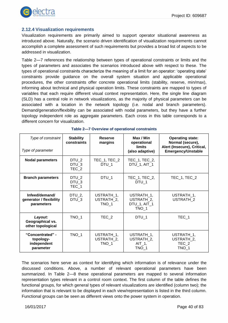
Project ID: 609687
16/01/2017 Page 40 of 83
Visualization requirements 2.12.4
Visualization requirements are primarily aimed to support operator situational awareness as
introduced above. Naturally, the scenario driven identification of visualization requirements cannot
accomplish a complete assessment of such requirements but provides a broad list of aspects to be
addressed in visualization.
Table 2—7 references the relationship between types of operational constraints or limits and the
types of parameters and associates the scenarios introduced above with respect to these. The
types of operational constraints characterize the meaning of a limit for an operator: ‘operating state’
constraints provide guidance on the overall system situation and applicable operational
procedures, the other constraints offer concrete operational limits (stability, reserve, min/max),
informing about technical and physical operation limits. These constraints are mapped to types of
variables that each require different visual context representation. Here, the single line diagram
(SLD) has a central role in network visualizations, as the majority of physical parameters can be
associated with a location in the network topology (i.e. nodal and branch parameters).
Demand/generation/flexibility can be associated with nodal parameters, but they have a further
topology independent role as aggregate parameters. Each cross in this table corresponds to a
different concern for visualization.
Table 2—7 Overview of operational constraints
Type of constraint
Type of parameter
Stability constraints
Reserve margins
Max / Min operational
limits (also adaptive)
Operating state: Normal (secure),
Alert (Insecure), Critical, Emergency/Unstable
Nodal parameters
DTU_2 DTU_3 TEC_2
TEC_1, TEC_2 DTU_1
TEC_1, TEC_2, DTU_1, AIT_1
Branch parameters
DTU_2 DTU_3 TEC_1
DTU_1 TEC_1, TEC_2, DTU_1
TEC_1, TEC_2
Infeed/demand/ generator / flexibility
parameters
DTU_2, DTU_3
USTRATH_1, USTRATH_2,
TNO_1
USTRATH_1, USTRATH_2, DTU_1, AIT_1
TNO_1
USTRATH_1, USTRATH_2
Layout: Geographical vs. other topological
TNO_1 TEC_2 DTU_1 TEC_1
“Concentrated” - topology-
independent parameter
TNO_1 USTRATH_1, USTRATH_2,
TNO_1
USTRATH_1, USTRATH_2,
AIT_1, TNO_1
USTRATH_1, USTRATH_2,
TEC_2 TNO_1
The scenarios here serve as context for identifying which information is of relevance under the
discussed conditions. Above, a number of relevant operational parameters have been
summarized. In Table 2—8 these operational parameters are mapped to several information
representation types relevant in a control room context. The first column of the table defines the
functional groups, for which general types of relevant visualizations are identified (column two); the
information that is relevant to be displayed in each view/representation is listed in the third column.
Functional groups can be seen as different views onto the power system in operation.
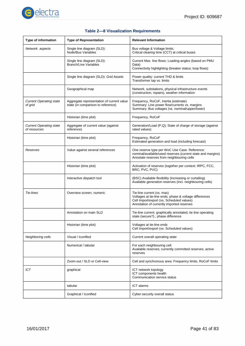
Project ID: 609687
16/01/2017 Page 41 of 83
Table 2—8 Visualization Requirements
Type of information Type of Representation Relevant Information
Network aspects Single line diagram (SLD): Node/Bus Variables
Bus voltage & Voltage limits; Critical clearing time (CCT) at critical buses
Single line diagram (SLD): Branch/Line Variables
Current Max. line flows; Loading-angles (based on PMU Data) Connectivity highlighting (breaker status; loop flows)
Single line diagram (SLD): Grid Assets Power quality: current THD & limits Transformer tap vs. limits
Geographical map Network, substations, physical infrastructure events (construction, repairs), weather information
Current Operating state of grid
Aggregate representation of current value state (in comparison to reference)
Frequency, RoCoF, Inertia (estimate) Summary: Line power flow/currents vs. margins Summary: Bus voltages (vs. nominal/upper/lower)
Historian (time plot) Frequency, RoCoF
Current Operating state of resources
Aggregate of current value (against reference)
Generation/Load (P,Q); State of charge of storage (against rated values)
Historian (time plot) Frequency, RoCoF Estimated generation and load (including forecast)
Reserves Value against several references One reserve type per WoC Use Case. Reference: nominal/available/used reserves (current state and margins) Annotate reserves from neighbouring cells
Historian (time plot) Activation of reserves (together per context: IRPC, FCC, BRC; PVC, PVC)
Interactive dispatch tool (BSC) Available flexibility (increasing or curtailing) Available generation reserves (incl. neighbouring cells)
Tie-lines Overview screen, numeric Tie-line current (vs. max) Voltages at tie-line ends; phase & voltage differences Cell Import/export (vs. Scheduled values) Annotation of currently imported reserves
Annotation on main SLD Tie-line current; graphically annotated; tie line operating state (secure?).; phase difference
Historian (time plot) Voltages at tie-line ends Cell Import/export (vs. Scheduled values)
Neighboring cells Visual / Iconified Current overall operating state
Numerical / tabular For each neighbouring cell: Available reserves; currently committed reserves; active reserves
Zoom-out / SLD or Cell-view Cell and synchronous area: Frequency limits, RoCoF limits
ICT graphical ICT network topology ICT components health Communication service status
tabular ICT alarms
Graphical / Iconified Cyber-security overall status
Project ID: 609687
16/01/2017 Page 42 of 83
3 Control room concepts sequence diagrams
3.1 Chapter outline
Following the control room scenario analysis conducted in Chapter 2, a number of scenarios is
selected and investigated further. Chapter 3 defines the control room flow of information for the
selected set of scenarios. Sequence diagrams are drawn in order to define information sent back
and forth between field and control room. Use cases invoked in specific control actions are
identified as well as actions that require manual intervention with the operator.
The latter activity is bridging the development and demonstration of decision support in the later
ELECTRA project phase.
3.2 Preventive transient stability (DTU_2)
The sequence diagram for preventive transient stability assessment is given in Figure 3—1. It
comprises two actors and four entities. The two actors are the cell operator and the balance
steering reserve provider. The four entities are the cell (WoC), the dispatchable units within a cell,
the SCADA system and the simulation software. The goal of the preventive transient stability
assessment is to ensure transient stability of the cell at all times, i.e. set preventive actions to
ensure a predefined transient stability level if too low transient stability margins are identified. The
predefined transient stability level is expressed as minimum critical clearing time (CCT) of a three-
phase fault, which should be respected throughout the whole system. That means the CCTs for
three-phase faults at every bus bar must be above the specified minimum CCT [30].
In the following a step-by-step explanation for the preventive transient stability assessment is
given. The SCADA system is updated with the current cell state, i.e. breaker status, set points of
generation unit. The simulation software contains a model of the network of the cell, which is
updated with the current cell state information from the SCADA system or from PMUs or from a
combination of both. Following the update of the cell state the simulation to assess the transient
stability can be carried out. Therefore, offline simulations for a set of different contingencies (e.g.
three-phase fault) have to be carried out. If issues are detected, i.e. the CCT of certain
contingencies is below the user-specific threshold (e.g. 200 ms), the needed dispatch to re-
establish the predefined stability margins is determined. The result of the assessment, including
the proposed dispatch and its associated additional generation costs is then presented to the
control room operator. The control room operator has to verify and confirm the proposed dispatch.
The operator has the ability to introduce additional constraints, such as unavailability of generators
to take over the dispatched power and get a new dispatch proposal considering the additional
constraints. If the capacity of the generators within the cell is insufficient to achieve the desired
stability limit, additional reserves can be requested from the balance steering provider. The whole
process runs in a loop where the maximum time of one iteration is limited to the activation of the
balance steering control.
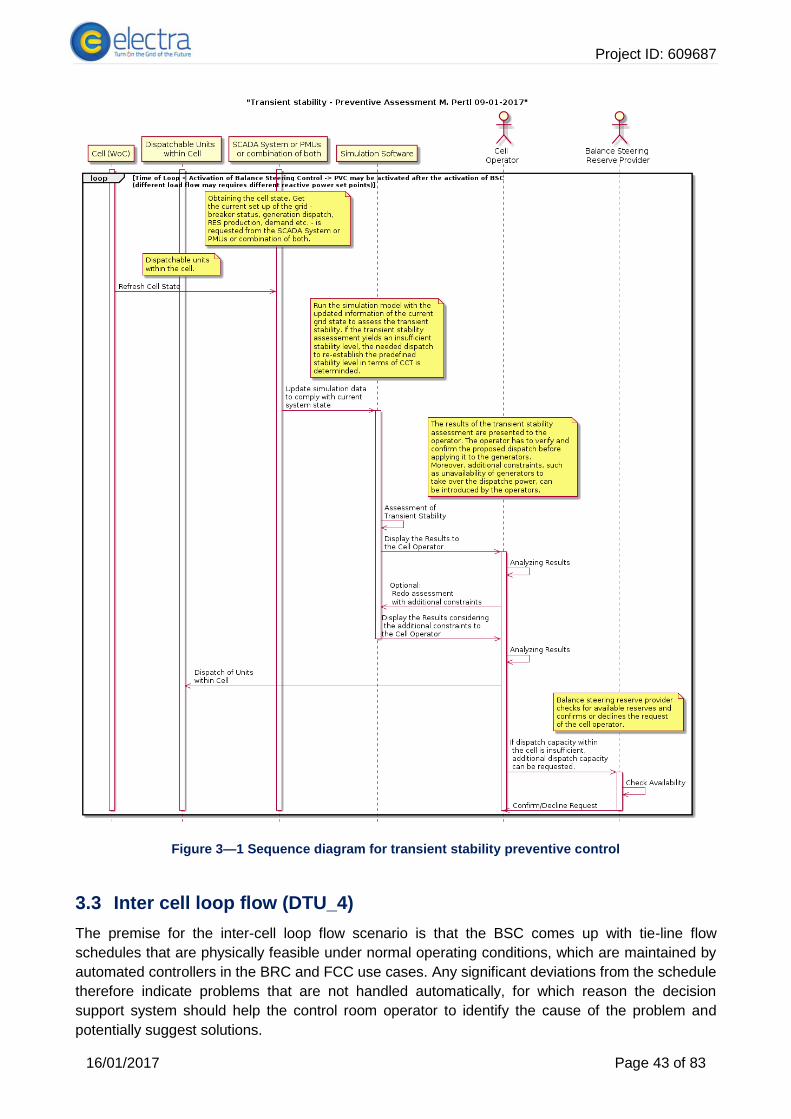
Project ID: 609687
16/01/2017 Page 43 of 83
Figure 3—1 Sequence diagram for transient stability preventive control
3.3 Inter cell loop flow (DTU_4)
The premise for the inter-cell loop flow scenario is that the BSC comes up with tie-line flow
schedules that are physically feasible under normal operating conditions, which are maintained by
automated controllers in the BRC and FCC use cases. Any significant deviations from the schedule
therefore indicate problems that are not handled automatically, for which reason the decision
support system should help the control room operator to identify the cause of the problem and
potentially suggest solutions.
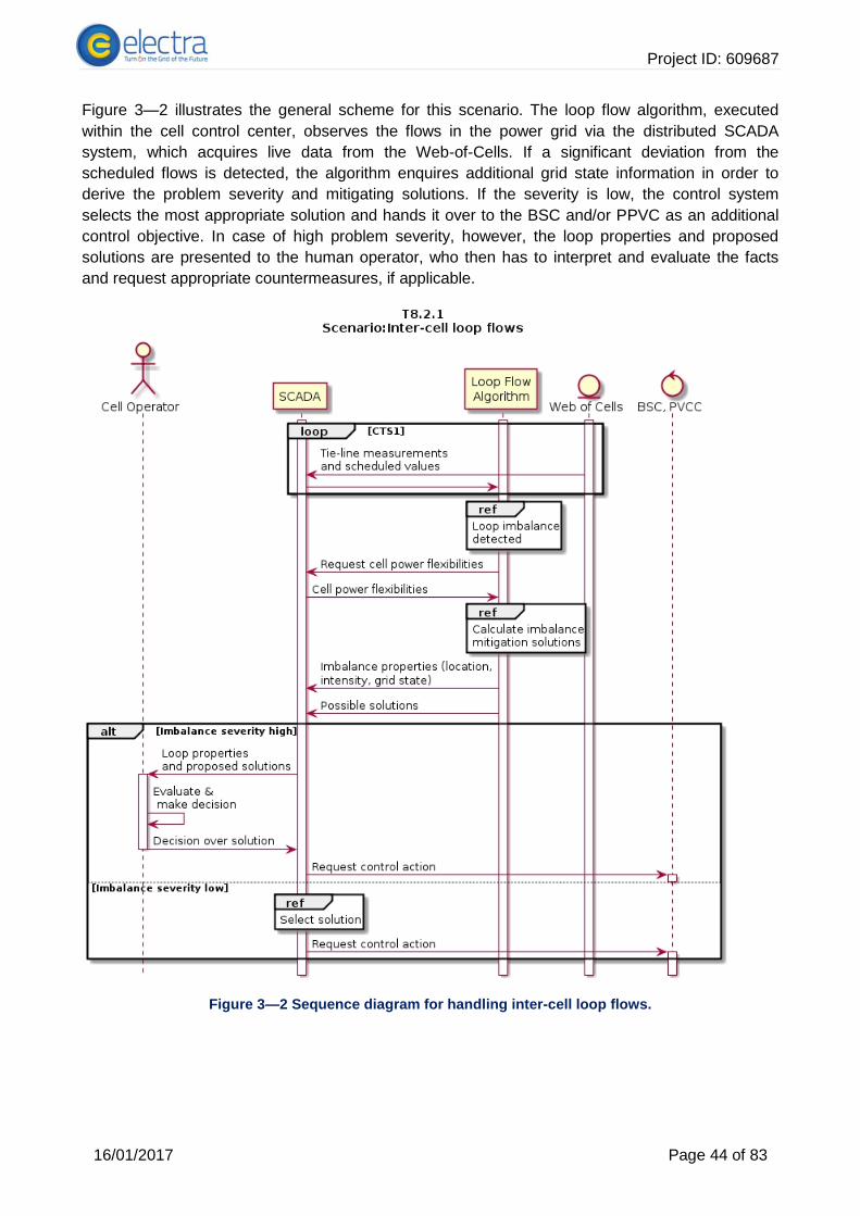
Project ID: 609687
16/01/2017 Page 44 of 83
Figure 3—2 illustrates the general scheme for this scenario. The loop flow algorithm, executed
within the cell control center, observes the flows in the power grid via the distributed SCADA
system, which acquires live data from the Web-of-Cells. If a significant deviation from the
scheduled flows is detected, the algorithm enquires additional grid state information in order to
derive the problem severity and mitigating solutions. If the severity is low, the control system
selects the most appropriate solution and hands it over to the BSC and/or PPVC as an additional
control objective. In case of high problem severity, however, the loop properties and proposed
solutions are presented to the human operator, who then has to interpret and evaluate the facts
and request appropriate countermeasures, if applicable.
Figure 3—2 Sequence diagram for handling inter-cell loop flows.

Project ID: 609687
16/01/2017 Page 45 of 83
3.4 Parameterization error detection of inverter-based DER (AIT_1)
In Figure 3—3, the detailed sequence diagram of the parameterization error detection approach
inverter-based DER (description see Section 2.6) is shown. In it, the main relationships between
actors and elements involved are represented by means of the information exchanges.
Through the cell monitoring (i.e., SCADA) system information (voltage, active and reactive power,
control parameter, etc.) on the DER controller status are provided to the cell operator. The cell
operator analyses and compares (either automatic or manual) the desired cell behaviour with the
cell observables and detects potential faults in the parameterization/configuration of the inverter-
based DER controller. Based on the nature of the faulty parameterization either a (i) re-
configuration of the controller parameters, (ii) an output limitation of the DER (active and reactive
power), or (iii) a disconnection of the DER can be the result in order to solve this issue.
Figure 3—3 Sequence diagram for detecting parametrization errors in inverter-based DER.
3.5 Normal operation until frequency collapse due to lack of system
inertia (TNO_1)
Due to the difficulties in implementing an indirect inertia monitoring scheme (see section 2.7 for
details), this section will utilize the direct monitoring method only.
To ensure system RoCoF during the worst case imbalance, is below the tripping threshold of the
frequency protection relays, inertia within the synchronous area must be coordinated. Each
resource (CTL0) reports its inertia capability regularly to the cell operator.
For simplicity it is assumed that there is a fixed frequency range that the grid is operated between
(e.g., 49 to 51 Hz). This can be used to define a worst case frequency range for virtual inertia
resources. This way each virtual resource does not need to inform the operator the state of charge
of its energy store. When it makes an offer for inertia and is deployed it guarantees the operator
that it has sufficient capacity to provide a full (e.g., 2Hz) inertial response during its deployment
window.
The cell operator can then summate all the values to determine the total inertia in the cell. This
value is communicated to the synchronous area inertia provision function at CTL3, where it can be

Project ID: 609687
16/01/2017 Page 46 of 83
summated together with the values from the other cells to determine the total inertia in the
synchronous area.
An estimate can be made of the worst case imbalance step that would likely occur. For simplicity
this can be assumed to be an n-1 scenario, i.e. tripping of the single largest generator or load.
Similarly the maximum allowable RoCoF can be estimated using the operator's knowledge of the
protection settings of generators that are currently dispatched. From this information the
synchronous area inertia provision function can calculate the inertia required from each individual
cell. The operators of each cell utilize its dispatch mechanism to deploy the most appropriate
individual resources as shown in Figure 3—4.
Figure 3—4 Sequence diagram for inertia coordination
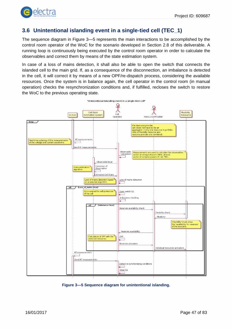
Project ID: 609687
16/01/2017 Page 47 of 83
3.6 Unintentional islanding event in a single-tied cell (TEC_1)
The sequence diagram in Figure 3—5 represents the main interactions to be accomplished by the
control room operator of the WoC for the scenario developed in Section 2.8 of this deliverable. A
running loop is continuously being executed by the control room operator in order to calculate the
observables and correct them by means of the state estimation system.
In case of a loss of mains detection, it shall also be able to open the switch that connects the
islanded cell to the main grid. If, as a consequence of the disconnection, an imbalance is detected
in the cell, it will correct it by means of a new OPF/re-dispatch process, considering the available
resources. Once the system is in balance again, the cell operator in the control room (in manual
operation) checks the resynchronization conditions and, if fulfilled, recloses the switch to restore
the WoC to the previous operating state.
Figure 3—5 Sequence diagram for unintentional islanding.
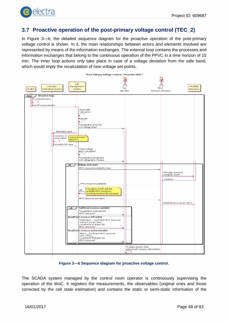
Project ID: 609687
16/01/2017 Page 48 of 83
3.7 Proactive operation of the post-primary voltage control (TEC_2)
In Figure 3—6, the detailed sequence diagram for the proactive operation of the post-primary
voltage control is shown. In it, the main relationships between actors and elements involved are
represented by means of the information exchanges. The external loop contains the processes and
information exchanges that belong to the continuous operation of the PPVC in a time horizon of 15
min. The inner loop actions only take place in case of a voltage deviation from the safe band,
which would imply the recalculation of new voltage set-points.
Figure 3—6 Sequence diagram for proactive voltage control.
The SCADA system managed by the control room operator is continuously supervising the
operation of the WoC. It registers the measurements, the observables (original ones and those
corrected by the cell state estimation) and contains the static or semi-static information of the
Project ID: 609687
16/01/2017 Page 49 of 83
network (topology, breakers’ status, etc.). On a fully automated basis, the control room operator
must be able to:
● compare the estimated cell state for the 15-minute horizon window with the limit values
● detect the abnormal condition in any node and launch a proactive optimal power flow (OPF)
process (if necessary)
● notify the cell operator and suggest solutions given the resources available
● send the new set-points to the local controllers in order to keep the voltages within the limits
established to optimize the system´s power flows.
3.8 Single frequency deviation event (USTRATH_1)
The sequence diagram report in Figure 3—7 represents the various interactions taking place
between the different system actors when a single frequency deviation event occurs. Arrows
indicate the flow of information between actors [31]. The descriptions of the actors are given below.
Aggregators/devices: This refers to the controllable demand/generation that is available within
the cell. In general, the aggregator is responsible for all devices that are present within their
portfolio. There can be more than one aggregator within a cell.
Cell Monitoring and Control (SCADA): This is the entity within the cell that is responsible for
monitoring the observables available within the network. Monitoring involves the processing of all
the observables to identify the disturbance location and magnitude. Control involves all the
automated control algorithms that are present within the cell.
Inter-cell Algorithm: This refers to the control algorithm that in a distributed manner
communicates and negotiates with other cells to coordinate frequency restoration and reserve
replacement plans.
Decision Support: Refers to the software system responsible for processing available information
to give the operator a plan for certain situations within the cell. It aids the operator with the
processing of cell issues by listing and prioritising the available options, and letting them select the
preferred action (supported operation). In addition, it allows the operator to take their own actions
(manual operation), and also allows the operator to delegate all decisions (fully automated
operation: the decision support system will enact the highest priority action).
Cell Operator: The person responsible for the secure and stable operation of the cell. Although
most of the functionalities within the cell are envisioned to be automated, manual control can be
given to the operator and their authority supersedes all other entities within the cell.
The sequence diagram is [VC1] concerned with the real-time operation phase within the problem cell
(i.e. the location of the disturbance). Therefore, it is assumed that at the start of the diagram, there
is an agreed plan for containment reserves and restoration reserves for the current scheduled
period, which has been communicated to devices as appropriate. The details of the scenario are
described below.
The process starts with the frequency deviation incident being detected locally at the cell level by
the Aggregator/Devices, where the frequency is monitored. The containment reserve plans are
automatically activated to contain the frequency. FCC is fast acting (within milliseconds) and so
there is no time for these events to be relayed to the operator, or for the operator to alter the plan.
However, the basis for the containment reserve plan is that its activation will contain a single
frequency deviation event.
Following this, the Cell Monitoring and Control attempts to identify the location of the incident to
prepare for the frequency restoration phase and BSC. Measurements are taken from within the
cell, and appropriate information shared with neighbouring cells, such as disturbance location.

Project ID: 609687
16/01/2017 Page 50 of 83
Figure 3—7 Sequence diagram for single frequency event
Once this process is complete, the problem cell is identified to the operator. The information
passed to the operator will differ depending on whether they operate the problem cell or not. If the
problem is within a distant cell, only an indication that there is a problem in the network currently
being resolved is needed, as no action from within this cell is necessary. A cell neighbouring the
problem cell will display a visualisation of how their reserves are contributing to the restoration of
the frequency. At this point the neighbouring cell can automatically calculate its available flexibility
over and above its current commitment so that it is already preparing for a subsequent incident
should that occur.
Project ID: 609687
16/01/2017 Page 51 of 83
The sequence diagram focuses on the cell where the problem originated. Therefore, it activates
the restoration plan for resolving this excursion. It is envisaged that a timeline visualisation
indicating the current frequency of the network and a forecast of the result of the restoration plans
is displayed to the human operator. This ensures that the operator is kept informed with what is
happening in the network, especially if it falls within their responsibility area. Finally, for the BSC
phase, a list of back-up resources available within the cell and neighbouring cells are provided to
the Decision Support. The Decision Support prioritises the resources and provides reserves
replacement options, giving the operator the chance to perform a manual selection from the
prioritised list. Once the options are presented to the Cell Operator, Decision Support will wait for a
period of time and then activate what it thinks is best. The time-line visualisations would also be
updated accordingly based on the operator selection, to reflect the new replacement reserves. The
operator has a certain window of time in which to make their decision, after which if no response
has been received, the decision support automatically signals the Cell Monitoring and Control to
implement its own plan.
It is worth mentioning here that for the single frequency event scenario, it can be seen that no
actions are really necessary from an operator’s point of view as everything is dealt with
automatically. Nevertheless, action can still be taken if needed to manually override the executed
plans.
3.9 Two simulation frequency events (USTRATH_2)
The second scenario, illustrated in Figure 3—8, starts with the same frequency containment
process as before, however a second frequency event occurs almost instantly within the same cell.
As there are insufficient containment reserves to deal with this excursion, load shedding takes
place to contain the frequency, and this information is passed to the operator. The same
disturbance location and magnitude identification process takes place as in USTRATH_1, with the
total combined disturbance from both events now being calculated. The deficit between the
reserves and the disturbance magnitude is provided to the decision support, and highlighted to the
operator [32].
As the load shed process has taken place by this point, there is some time available to send
requests to the neighbouring cells for available back-up resources. This available resources
information from the problem cell and neighbouring cells is sent to Decision Support, which
formulates a prioritised list of the restoration options to operator. There is a time window for the cell
operator to make their decisions, after which frequency restoration is enacted either by utilising the
decision support’s top ranked plan or the operator’s decision. This is achieved by the Decision
Support sending a signal to Cell Monitoring and Control to procure the resources. Once resources
are procured, the full frequency restoration process can be completed and the visualisations
showing the time-line of frequency of the network can be updated accordingly. Finally, the
frequency reserve replacement will be achieved using the same operations as in the previous
scenario (USTRATH_1).

Project ID: 609687
16/01/2017 Page 52 of 83
Figure 3—8 Sequence diagram for two frequency events within the same cell

Project ID: 609687
16/01/2017 Page 53 of 83
4 Visualization strategy approaches
4.1 Chapter outlines
The aim of this chapter is to report examples of visualizations based on the different scenarios
investigated in the previous stages of this task. The outcome of the stakeholder interaction carried
out during the CIRED workshop 2016 is reported as well.
4.2 Foreword on visualization strategy and outcome of the interaction
with stakeholders
The control of a power system starts with an effective visualization strategy of the most important
states of the system. Due to the complexity of modern power systems however, an enormous
amount of information is required in order to properly observe and derive system values (see
Figure 4—1). It is necessary to display at a glance all information, while trying to keep the decision
process as smooth and simple as possible due to the fact that humans are bad multi-taskers.
Figure 4—1 Example of TSO control room (National grid, UK)
In order to define an effective visualization strategy for the arising web-of-cell concept, interaction
with stakeholders took place with a dedicated session at the CIRED workshop 2016 (14-15 June,
Helsinki). The main outcome and discussions points are reported in this paragraph and form the
basis for the rest of the visualization chapter.
The main point is therefore defining how much information the cell operator needs to know. Is there
the need to continuously view all the details of what is going in the cell or just the general status is
sufficient (e.g. the n-1 is verified, frequency and all voltages are within limits) in case nothing is
wrong, and only “need to know” information in case something is not right?
The recommendation would be to show “Need to know” Information at different control topology
levels (CTLs), providing a straight guidance from signalled problem to the root cause. In order to

Project ID: 609687
16/01/2017 Page 54 of 83
do that potential corrective actions need to be suggested to the operator as previously discussed in
the previous chapter while providing the time sequence diagram for the selected pool of scenarios.
Concerning the high level representation of the power system, which one is more suitable for the
operator?
The recommendation is to have the possibility of representing the power system as interconnected
cells, which are represented with a traffic light approach (i.e. green if there are not issues, yellow if
there are critical conditions, red if there are issues). Synthetic cell information is displayed on each
cell and the operator can zoom in each cell for further details.
On the other hand, less interest is on having the power system represented with a single line wiring
diagram, where the elements (e.g. branch, nodes etc.) experiencing issues (e.g. overcurrent,
overvoltage etc.) are evidenced with a traffic light approach as illustrated in Figure 4—2.
Figure 4—2 Traffic light approach for visualizing the WoC
Table 4—1 is summing up the results on the individual questions regarding on which kind of
information should be displayed to the operator respectively on a high-level view of the WoC and
on a zoomed view. For each field, an indication on whether the information should be Mandatory,
Optional or Not necessary is given.
Concerning the network representation, the single line diagram should be available in the detailed
view of the cell, while a geographical/abstract map should be mandatory on a high level view. With
reference to the current status of the cell, frequency, load and generation values are mandatory on
a high level, while, bus voltages and line power and currents are mandatory on detailed level.
Strangely enough inertia, state of charge levels and rated values of components are not deemed
necessary.
With reference to the reserve instead, only generation and storage are of interest, while load and
inertia flexibility are optional. In any case in a detailed view of the cell, none of the reserve value is

Project ID: 609687
16/01/2017 Page 55 of 83
considered mandatory. As per the cell interconnection, power exchange is considered always
mandatory, while the voltages at the tie line ends are optional. Current values are mandatory only
in the detailed view.
When it comes to neighbouring cells, their status and reserve is deemed necessary only in a
detailed view, while they are considered optional on a high level. ICT information is valued optional
on the high level view; however, it is seen as mandatory information at detailed view.
Table 4—1 Information that should be displayed
M = mandatory; O = optional; N = not necessary
Type of information High level (Cell) Low Level (detailed view of the cell)
Network representation Single line diagram O M
Geographical map M O
current status Frequency M N
RoCoF M N
Generation M O
Load M O
State of charge of storage
O O
Inertia O O
Line power flows N M
Line currents N M
Bus voltages N M
Rated values of components
N O
Reserves (nominal/available/used)
Generation M O
Load flexibility O O
Storage M O
Inertia O O
Tie-lines Exchanged power M M
current O M
Voltages at tie-line ends O O
Neighboring cells Status O M
Reserves O M
ICT ICT network topology O M
ICT components health O M
Communication services O M
4.3 Visualization inertia allocation and exchange of inertia response
power
Conventional visualizations for network operators are complex SCADA systems which present all
information simultaneously in parallel. This visualization approach not only makes it difficult to
identify issues arising, but also to react appropriately. With the web-of-cell concept we look to
increase decentralized control for smart grid services on all levels of the synchronous area.
Therefore, a simplification of visuals to reduce reaction times and monitor the cell as well as the
synchronous area is proposed. For simplicity and congruence with TNO’s use case this
visualisation only considers coordination of inertia.
The ELECTRA proposition is to have a two layered perspective, of the synchronous area and the
cell area. Each layer has limited, necessary information with three panels. For the synchronous

Project ID: 609687
16/01/2017 Page 56 of 83
area the resource and cell states as well as a circuit diagram of the synchronous area. For the cell
area, the devices and resource states as well as a circuit schematic will have visualization panels.
See Figure 4—3 for general overview of visualization structure.
Figure 4—3 Architectural overview of inertia allocation
The lines in Figure 4—3 show the information flow for the visualization model (GUI made in
GUIDE) to monitor the system and not the control of the cells themselves. The colours of the boxes
are assigned per control level, the orange being synchronous area, and light grey is the cell area,
with dark grey being the final deployment. The green arrows are inputs, state information and
device information of the loads and generations in the controlled area to the circuit diagram. So for
example, for the Cell area, CTL 2, the device states, e.g. power, and resource states, e.g.,
available inertia, reactive and active power will be input into the diagram. This is to enable the cell
operator to see the location of the issue, if one arises.
A parented view at the synchronous and cell level provides an overview of the current state of the
network. The health of the system will be represented by colours and revealing further information
when necessary as indicated in Figure 4—4. Green = Normal, Yellow = Warning, Red = Error. If
an error or warning appears then the control room operator will be automatically guided to the root
of the problem at a CTL-2 and CTL-1 level. Corrective actions can be a combination of manual and
automated depending on the issue.

Project ID: 609687
16/01/2017 Page 57 of 83
Figure 4—4 Synchronous area state visuals
Additionally, cell states (see Figure 4—5) and schematics will be available in separate visuals of
the synchronous area. Similarly to Figure 4—4, detailed state visuals are also provided for each
cell.
Figure 4—5 Cell state panel overview
From the cell state resource panel, a specific cell can be visualized with its own resource panel as
well a schematic. It should be noted that upon detecting a warning or emergency state the cell
which is impacted will automatically appear for the network operator with resource options
available in a merit order list.

Project ID: 609687
16/01/2017 Page 58 of 83
4.4 Visualization clues for unintentional islanding detection and
upcoming voltage control
Nowadays, the cell operators are used to visualize their power systems by using complex SCADA
systems. For example, the Spanish TSO, Red Eléctrica de España, is equipped with two parallel
centers in operation, named (CECOEL). CECOEL is in charge of supervising the grid security by
observing in real-time the grid status as well as the electrical parameters, acting over the control
variables to keep the security of supply or to restore the service after an incident. This system, as
an example of one most advanced control and visualization centers, is very effective. It is able to
manage 25.000 digital signals and 21.000 analog signals in cycles of 4, 8 and 12 seconds (this
means a sample rate of 0.25Hz, 0.5Hz or 0.75Hz). Nevertheless, the extension of this philosophy
to the WoC can be insufficient due to the excess of signals that would come up as a consequence
of the generation decentralization.
The challenge for visualizing the WoC lies on determining which variables should be visualized by
the Cell Operator according to the system status, to find a trade-off between the information
required to keep the system security and the data management issues (number of signals,
samplings, etc.)
An exemplary visualization approach in the Matlab/Simscape environment has been developed
within this task, only with illustrative purposes. In order to follow the visualization sequence, it has
been applied to the SPRS (TEC-base) grid for representing the scenarios TEC-1 (unintentional
islanding event in a single-tied cell) and TEC-2 (proactive operation of the post-primary voltage
control).
A global picture of the system view at the upper level (CTL-3) is shown in Figure 4—6.
Figure 4—6 CTL-3 view
C-A and C-B represent the groups of cells under the responsibility of cell operator A and cell
operator B respectively. The independent cell monitoring systems of C-A have been grouped into a
single block for simplification purposes.
At the CTL-3 level, the information that has to be known by the operator is the status of the cell by
means of an area-tie line diagram, with led indicators:
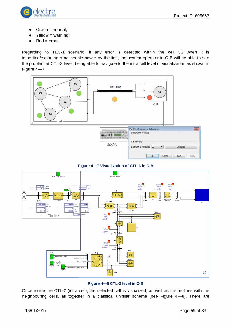
Project ID: 609687
16/01/2017 Page 59 of 83
● Green = normal;
● Yellow = warning;
● Red = error.
Regarding to TEC-1 scenario, if any error is detected within the cell C2 when it is
importing/exporting a noticeable power by the link, the system operator in C-B will be able to see
the problem at CTL-3 level, being able to navigate to the intra cell level of visualization as shown in
Figure 4—7.
Figure 4—7 Visualization of CTL-3 in C-B
Figure 4—8 CTL-2 level in C-B
Once inside the CTL-2 (intra cell), the selected cell is visualized, as well as the tie-lines with the
neighbouring cells, all together in a classical unifiliar scheme (see Figure 4—8). There are
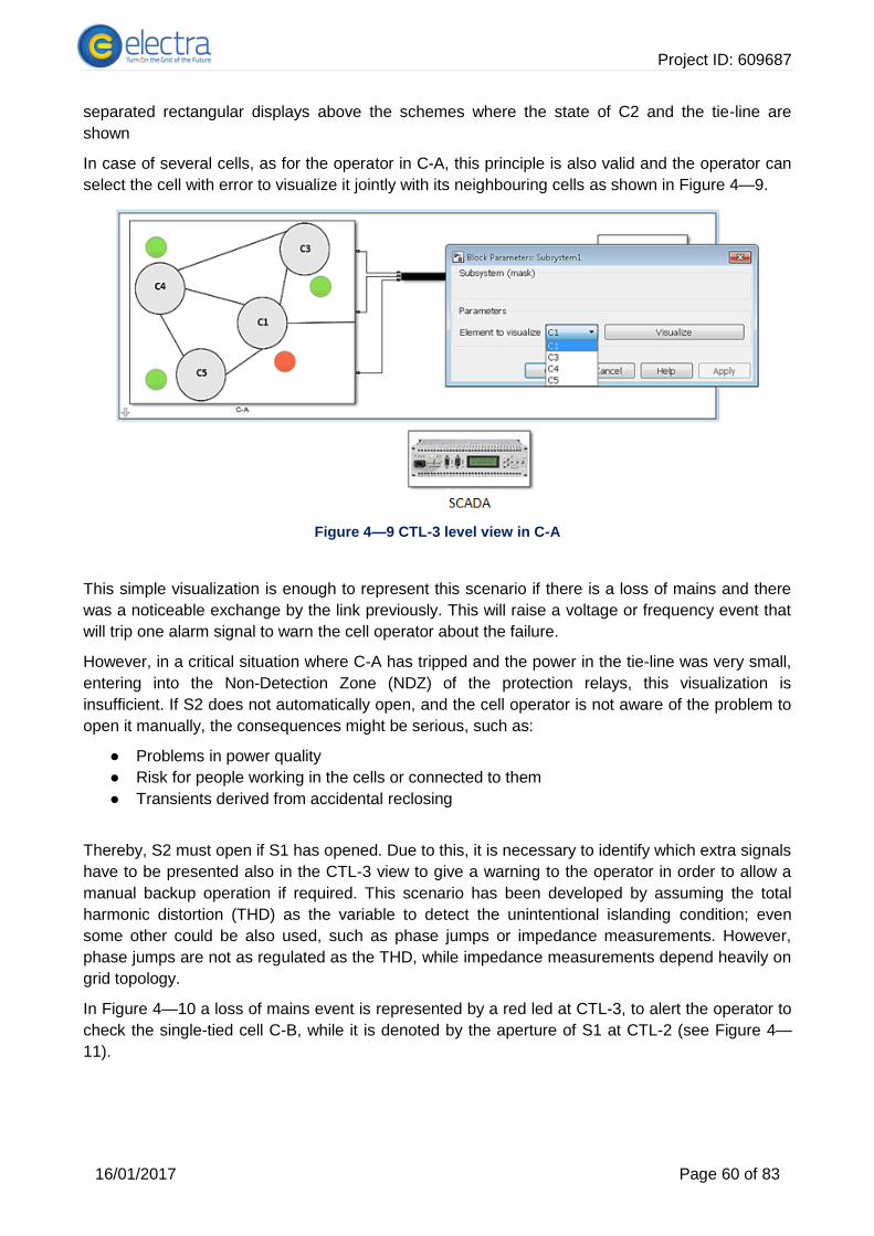
Project ID: 609687
16/01/2017 Page 60 of 83
separated rectangular displays above the schemes where the state of C2 and the tie-line are
shown
In case of several cells, as for the operator in C-A, this principle is also valid and the operator can
select the cell with error to visualize it jointly with its neighbouring cells as shown in Figure 4—9.
Figure 4—9 CTL-3 level view in C-A
This simple visualization is enough to represent this scenario if there is a loss of mains and there
was a noticeable exchange by the link previously. This will raise a voltage or frequency event that
will trip one alarm signal to warn the cell operator about the failure.
However, in a critical situation where C-A has tripped and the power in the tie-line was very small,
entering into the Non-Detection Zone (NDZ) of the protection relays, this visualization is
insufficient. If S2 does not automatically open, and the cell operator is not aware of the problem to
open it manually, the consequences might be serious, such as:
● Problems in power quality
● Risk for people working in the cells or connected to them
● Transients derived from accidental reclosing
Thereby, S2 must open if S1 has opened. Due to this, it is necessary to identify which extra signals
have to be presented also in the CTL-3 view to give a warning to the operator in order to allow a
manual backup operation if required. This scenario has been developed by assuming the total
harmonic distortion (THD) as the variable to detect the unintentional islanding condition; even
some other could be also used, such as phase jumps or impedance measurements. However,
phase jumps are not as regulated as the THD, while impedance measurements depend heavily on
grid topology.
In Figure 4—10 a loss of mains event is represented by a red led at CTL-3, to alert the operator to
check the single-tied cell C-B, while it is denoted by the aperture of S1 at CTL-2 (see Figure 4—
11).

Project ID: 609687
16/01/2017 Page 61 of 83
Figure 4—10 Loss of mains event at CTL-3 level
Figure 4—11 Loss of mains event at CTL-2 level
As can be seen in Figure 4—11 the differences in frequency and voltage are smaller than the
detection thresholds of the relays, so S2 does not automatically open, despite the loss of mains
event at C-A. However, after the S1 opening, the THD in the tie-line and in C2 has boosted,
leading to the detection of the event, which is visualized by a red led indicator at CTL-3. The
visualization of voltage, frequency, sequence and THD in CTL-2 will help the cell operator in his
decision process to manually open the switch S2.
Once the mains has come back (C-A), the resynchronization conditions are checked in order to
automatically or manually close S2 only when fulfilled (see Figure 4—12).
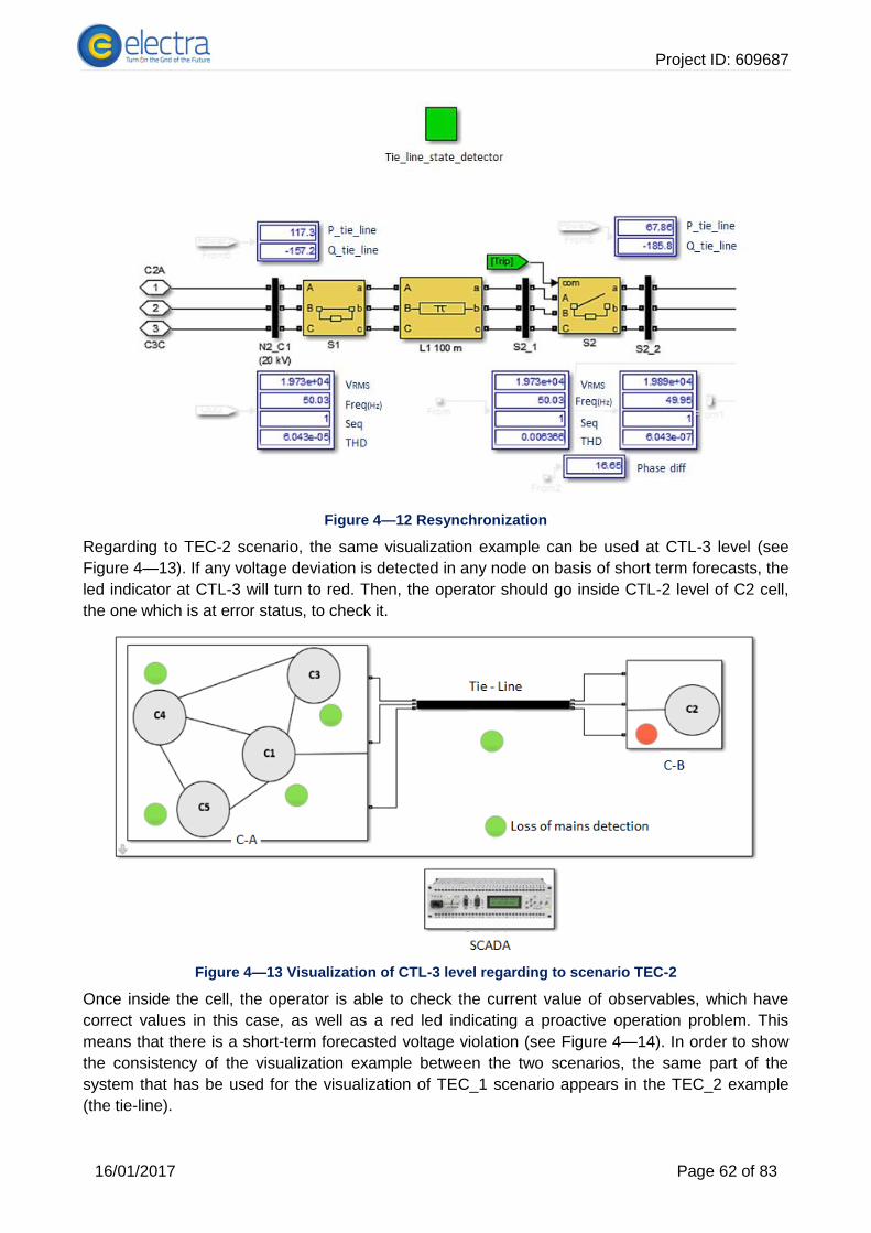
Project ID: 609687
16/01/2017 Page 62 of 83
Figure 4—12 Resynchronization
Regarding to TEC-2 scenario, the same visualization example can be used at CTL-3 level (see
Figure 4—13). If any voltage deviation is detected in any node on basis of short term forecasts, the
led indicator at CTL-3 will turn to red. Then, the operator should go inside CTL-2 level of C2 cell,
the one which is at error status, to check it.
Figure 4—13 Visualization of CTL-3 level regarding to scenario TEC-2
Once inside the cell, the operator is able to check the current value of observables, which have
correct values in this case, as well as a red led indicating a proactive operation problem. This
means that there is a short-term forecasted voltage violation (see Figure 4—14). In order to show
the consistency of the visualization example between the two scenarios, the same part of the
system that has be used for the visualization of TEC_1 scenario appears in the TEC_2 example
(the tie-line).
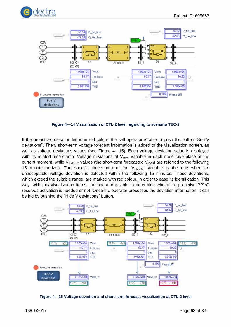
Project ID: 609687
16/01/2017 Page 63 of 83
Figure 4—14 Visualization of CTL-2 level regarding to scenario TEC-2
If the proactive operation led is in red colour, the cell operator is able to push the button “See V
deviations”. Then, short-term voltage forecast information is added to the visualization screen, as
well as voltage deviations values (see Figure 4—15). Each voltage deviation value is displayed
with its related time-stamp. Voltage deviations of VRMS variable in each node take place at the
current moment, while VRMS-ST values (the short-term forecasted VRMS) are referred to the following
15 minute horizon. The specific time-stamp of the VRMS-ST variable is the one when an
unacceptable voltage deviation is detected within the following 15 minutes. Those deviations,
which exceed the suitable range, are marked with red colour, in order to ease its identification. This
way, with this visualization items, the operator is able to determine whether a proactive PPVC
reserves activation is needed or not. Once the operator processes the deviation information, it can
be hid by pushing the “Hide V deviations” button.
Figure 4—15 Voltage deviation and short-term forecast visualization at CTL-2 level

Project ID: 609687
16/01/2017 Page 64 of 83
To summarize, this visualization example proposes adding the following elements and magnitudes
with the aim of enhancing the voltage control at network operation, avoiding an overdose of
information:
● At CTL3 level, one led to display a potential loss of mains, in addition to those ones
displaying the state of cells and tie-lines
● At CTL2 level, the integration of THD and the possibility of see the short-term forecasted
voltage violations, including a led to be aware of proactive operation problems, along with
the classical magnitudes, such as present voltage, power, frequency, sequence or PPVC
reserves status.
4.5 Decentralised topology and power system state visualisation
Established SCADA implementations are a bottleneck for decentralised control as envisioned with
ELECTRA’s Web-of-Cells concept. Traditionally, communication links in SCADA systems are
statically configured for each observed and controlled device. Changes in the system, like added or
removed devices, must be entered manually in a database along with the corresponding network
diagram. The rising number of DERs and metering devices distributed throughout all levels of the
electric power grid render make this task increasingly tedious and error-prone, and also data
bandwidth has to be taken into account. Already today, measurements with high sample rates such
as from phasor measurement units (PMUs) are usually first collected and filtered in phasor data
concentrators (PDCs) before they are passed on to control centres. Data acquisition in future
SCADA systems will be highly decentralised and new visualisation concepts are necessary to
accommodate for the dynamic environment and provide the control room operators relevant
information.
The so-called observability platform presented in [33] and [34] interfaces energy devices to an
abstraction layer, over which the abstract device representations (agents) exchange data. The
communication model is based on dynamic point-to-point (P2P) connections, which can be
established and closed on demand much like in the TCP/IP protocol. An application layer, used for
the presented network visualisation concept, provides access to an agent’s database holding
knowledge of its environment. The premise for visualising the grid state is the absence of a central
topology processor, and all the agents possess only knowledge about their physical connections
and logical assignments. Agents can query other agents for their state and topological knowledge
and by that extend their view on the grid.
This grid visualisation as developed within this task is a dynamically built graph containing
information and elements relevant to the selected perspective on the system. New perspectives
can be opened with a click, such as:
● Inter-cell view: This is the top-level view on the network that shows cells and tie-lines
running between them.
● Intra-cell view: Shows buses and lines within a cell, as well as the tie-lines and
corresponding neighbouring cells.
● Local view: Here, the devices and lines connected to one bus along with its associated cell
are presented to the operator.
● Global physical view: The buses and lines of the entire grid are shown as a graph.
The visualisations come with several overlays that can be turned on or off. Physical grid
connections (i.e., lines) between cells and/or buses are visible by default, whereas the following
overlays are optional:
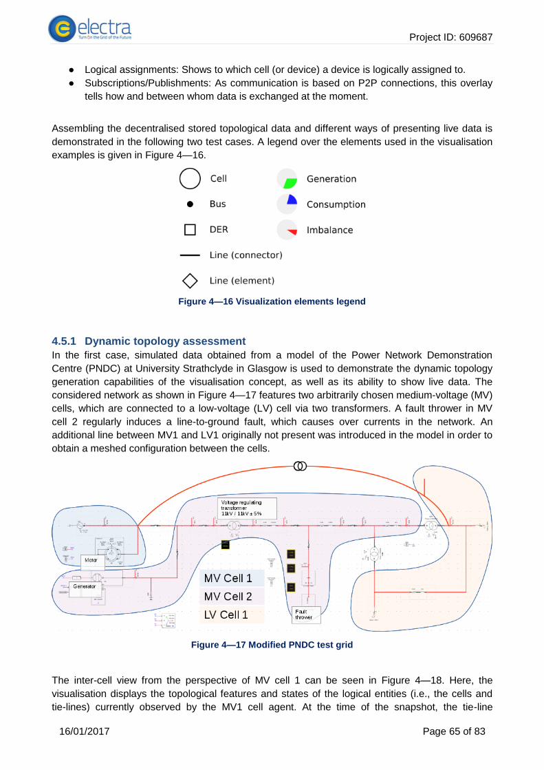
Project ID: 609687
16/01/2017 Page 65 of 83
● Logical assignments: Shows to which cell (or device) a device is logically assigned to.
● Subscriptions/Publishments: As communication is based on P2P connections, this overlay
tells how and between whom data is exchanged at the moment.
Assembling the decentralised stored topological data and different ways of presenting live data is
demonstrated in the following two test cases. A legend over the elements used in the visualisation
examples is given in Figure 4—16.
Figure 4—16 Visualization elements legend
Dynamic topology assessment 4.5.1
In the first case, simulated data obtained from a model of the Power Network Demonstration
Centre (PNDC) at University Strathclyde in Glasgow is used to demonstrate the dynamic topology
generation capabilities of the visualisation concept, as well as its ability to show live data. The
considered network as shown in Figure 4—17 features two arbitrarily chosen medium-voltage (MV)
cells, which are connected to a low-voltage (LV) cell via two transformers. A fault thrower in MV
cell 2 regularly induces a line-to-ground fault, which causes over currents in the network. An
additional line between MV1 and LV1 originally not present was introduced in the model in order to
obtain a meshed configuration between the cells.
Figure 4—17 Modified PNDC test grid
The inter-cell view from the perspective of MV cell 1 can be seen in Figure 4—18. Here, the
visualisation displays the topological features and states of the logical entities (i.e., the cells and
tie-lines) currently observed by the MV1 cell agent. At the time of the snapshot, the tie-line

Project ID: 609687
16/01/2017 Page 66 of 83
between MV1 and MV2 is reported to be overloaded due to the line-to-ground fault, for which
reason the line is marked red.
Figure 4—18 Inter cell view of cell MV1
A click on the circle representing cell MV2 opens the intra-cell view. The agent running the
visualisation (MV1 cell agent) queries at this point the MV2 cell agent for its logically assigned
devices and receives back a list of device identifiers. Subsequently, the agent requests the
corresponding devices to transmit their topological knowledge, which allows the MV1 agent to
assemble the local topology as depicted in Figure 4—19. Now, the internal configuration of the
MV2 cell can be inspected, which reveals for example how the two interconnections between MV2
and LV2 are set up. In addition, the contacted devices start publishing their state to the MV1 cell,
which shows in detail the lines affected by the fault.

Project ID: 609687
16/01/2017 Page 67 of 83
Figure 4—19 Intra-cell view of cell MV2 as observed by the MV cell 1 agent
The local view of the MV2 cell agent is given in Figure 4—20. In this perspective the assigned
electric lines are painted as discrete elements instead of edges between the bus nodes in order to
show them even if they are physically not connected (e.g., because of open breakers). Lines
connected to other cells mark visually cell borders, this allowing observing them at a glance.
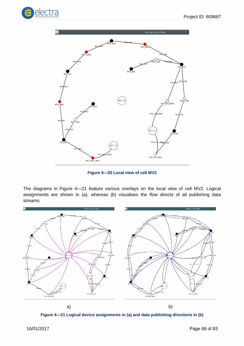
Project ID: 609687
16/01/2017 Page 68 of 83
Figure 4—20 Local view of cell MV2
The diagrams in Figure 4—21 feature various overlays on the local view of cell MV2. Logical
assignments are shown in (a), whereas (b) visualises the flow directs of all publishing data
streams.
a) b)
Figure 4—21 Logical device assignments in (a) and data publishing directions in (b)

Project ID: 609687
16/01/2017 Page 69 of 83
Finally, also a global topological view can be obtained by querying all cells for their underlying
topologies. Figure 4—22 shows the graph-like result of the considered grid with all buses as nodes
and lines as edges.
Figure 4—22 Global topology view
SYSLAB layout for market-based power matching algorithm 4.5.2
As part of the technical demonstrations for the PowerlabDK inauguration ceremony (Lyngby, 24
June 2016), the SYSLAB simulation model at the Technical University of Denmark shown in Figure
4—23 was used to demonstrate a market-based power matching algorithm. The visualisation
framework developed within this task served as a tool to observe the grid state in real-time, for
which reason power balances were particularly highlighted.
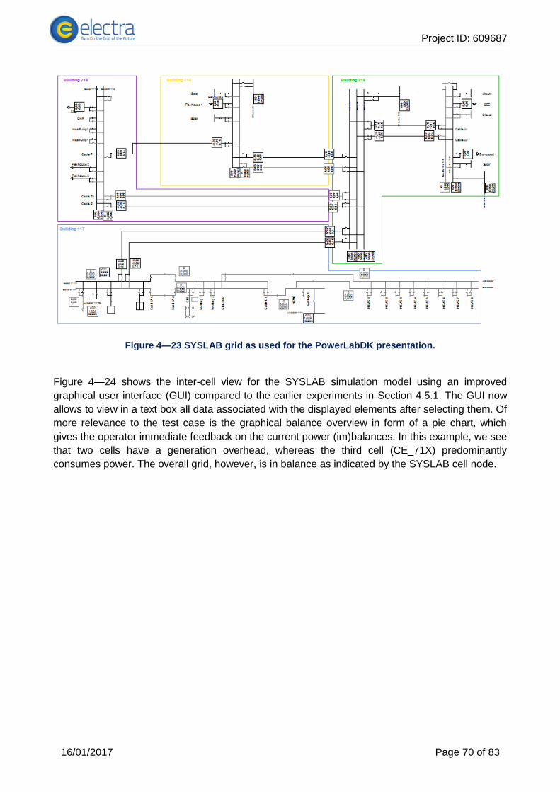
Project ID: 609687
16/01/2017 Page 70 of 83
Figure 4—23 SYSLAB grid as used for the PowerLabDK presentation.
Figure 4—24 shows the inter-cell view for the SYSLAB simulation model using an improved
graphical user interface (GUI) compared to the earlier experiments in Section 4.5.1. The GUI now
allows to view in a text box all data associated with the displayed elements after selecting them. Of
more relevance to the test case is the graphical balance overview in form of a pie chart, which
gives the operator immediate feedback on the current power (im)balances. In this example, we see
that two cells have a generation overhead, whereas the third cell (CE_71X) predominantly
consumes power. The overall grid, however, is in balance as indicated by the SYSLAB cell node.

Project ID: 609687
16/01/2017 Page 71 of 83
Figure 4—24 Inter-cell view on the SYSLAB simulation model
Selecting the intra-cell view for cell CA_71X reveals that it consists of two buses, one only
consuming power and one mostly producing, as shown in Figure 4—25.
Figure 4—25 Intra-cell view of cell CA_71X
Going even further down in the hierarchy exposes the devices that actually contribute to the overall
power mix, as exemplified on bus BA_715 in Figure 4—26. Here we see that Gaia (a wind turbine)

Project ID: 609687
16/01/2017 Page 72 of 83
and the solar cells are generating electric power, whereas a little part is consumed by the
Flexhouse (an office building equipped with power meters). Potential applications of having this
information available at hand could be checking if the devices report the right data (e.g., generating
and consuming devices should report data with opposite signs), or combining the electricity output
with weather information to see if devices work as they are supposed to under given conditions.
Figure 4—26 Local physical view of bus BA_715
SYSLAB layout for individual and combined Use cases validation to be 4.5.3
carried out in ELECTRA lab-scale proof of concept activities
Within WP7 of ELECTRA, laboratory validation of use cases is about to begin and the following 4-
cell layout will be used as reference test grid for some of the UC (both individual UC and
combinations of UC). Depending on the type of use case under test, several areas of the
laboratory (namely cell 1, cell 2 and cell 3) will be used. More detailed information about the
different experiments will be reported in D7.2, at this stage, the mere visualization of the single
diagram and the simplified representation of the different power components is reported in Figure
4—27.

Project ID: 609687
16/01/2017 Page 73 of 83
Figure 4—27 Single diagram and simplified representation of different power components
Project ID: 609687
16/01/2017 Page 74 of 83
5 Conclusions and future work
Scenarios for deriving new future control functionality in the Web-of-Cells framework have been
introduced and analysed to derive concrete visualization requirements for operator support for a
Web-of-Cells based grid operation. The work started after the overview on requirements on future
control rooms based on general trends emerging in power system operation described in the
internal report 8.1 and summarized in Chapter 1 of the present deliverable. Since roles and
activities in the future control centres will evolve with respect to the manual switching, dispatching
and restoration functions currently active, a set of requirements capturing those needs was
distilled. The control room operator will need a topological view of the system states and a
measure of active controllers. Given the distributed nature of the control system and the
dependencies between electrical and informatics systems, status of the ICT network needs to be
displayed on a need to know basis. Due to the involvement of numerous and distributed energy
sources, an aggregated status of deployed and available reserve (in term of active and reactive
power primarily, but also in term of other relevant system parameters as for instance SOC of
storages or inertia) on different areas need to be given. Finally, because of the interconnected
nature of the power system and due to the mutual interdependencies among different voltage
levels, distilled information on reserves and limits of neighbouring areas is necessary in order to
securely operate each Cell.
In view of the ELECTRA WoC concept, the operator task is to supervise a highly automated power
system where there must be possibility and the capacity to intervene if necessary.
A clear link with the WoC concept, including use cases defined in the ELECTRA deliverables D3.1
and D6.1 is established by means of future control room scenarios. The scenarios have been
compiled to create an overview of possible situations in future power systems which are viewed as
controlled by the ELECTRA Web-of-Cells approach. Three types of scenarios are analysed:
scenarios that challenge traditional control schemes in power systems with increasingly distributed
and renewable energy resources, scenarios that caused major failures (i.e., blackouts) and
scenarios that can be expected in the future in a WoC context.
The operator support functions provided in the control room have been divided into three aspects:
● System monitoring: operator situational awareness; evaluation of what is critical right now
● Supervisory control and interventions: offer input for operators to adjust system state
● Decision support: help operators identifying the right intervention
Whereas the objectives for WoC (coordinated) control functions addressed decomposed sub-
problems of the power system, concerning future control room functionality, the task was to
present a common view of the automated power system state, including the state of both the
physical variables as well as the operation of control functions and objectives. The objective of
outlining these scenarios has been therefore to identify specific requirements for visualization,
analytics and decision support. A systematic approach to such requirements analysis for human
machine interactions has been developed as Cognitive Systems Engineering. On this background,
an analysis methodology called “cognitive work analysis” (CWA) has been applied, which offers a
stepwise methodology for systematically identifying and constructing a knowledge context in which
this relevant information have been described.
In adopting this methodology for the purpose of the control room analysis, a first step was therefore
to describe how the system (the work domain) ‘looks’ from the operator point of view: describing
the operating objectives, power system and control functions at several levels of detail. While a
Project ID: 609687
16/01/2017 Page 75 of 83
hierarchically organized analysis of the operator’s decision-making was employed for Step 2
(activity or control task analysis).
A cross-sectional analysis of the above scenarios to reflect the coverage of the investigated
scenarios with respect to possible future situations, network levels and topologies, and the WoC
automatic control systems is reported and subsequently requirements have been drawn. According
to the analysis of operational constraints, the following requirements can be derived in term of
enhanced visualization and decision support features:
R-N-1 Stochastic influence of RES on tie-line flows causes uncertain deviations from scheduled
exchange which must be considered in the planning of secure exchange schedules (applies to AC-
tie lines, with consideration of special cases of radial and meshed operation).
R-N-2 A high share of converter-based generation reduces rotational synchronous inertia, which
makes it necessary to monitor overall available inertia (applies to synchronous region).
R-N-3 Physical power flows are not governed by cell- and market- defined (conceptual) system
boundaries, which means that exchanges across such abstract system boundaries will mismatch
the physical power flow (applies to cells interconnected by multiple tie-lines and with meshed
structure); physical network models are therefore required to evaluate security of planned
exchange schedules.
R-N-4 Coordinated operation of point-to-point and multi-terminal DC grids to support and increase
stability of AC grids.
The control room pragmatic approach has then been further pursued, where the control tasks were
analysed in terms of a sequence analysis, accounting both for required decisions and analytics and
the required information exchange. Such an annotated sequence diagram therefore addressed
aspects of steps 3 (mental strategies) and 4 (social organisation) in the CWA methodology
previously outlined. For a selected pool of scenarios the sequence of information, sequence
diagrams have been defined in order to specify the information sent back and forth between field
and control room. Use cases invoked in specific control actions are identified as well as actions
that require manual intervention with the operator. The outcome of this chapter is used as basis for
the decision support activity in a subsequent project task (T8.3 development and demonstration of
decision support).
In the final part, starting from the scenarios analyses as well as discussions and interactions with
different stakeholders (specifically DSOs and TSOs) at the last CIRED 2016 workshop, different
examples of visualization have been presented. The possibility of representing the power system
as interconnected cells was confirmed and suggested to extend the operational representation by
a traffic light approach (i.e., green if there are not issues, yellow if there are critical conditions, red if
there are issues). Synthetic cell information is displayed on each cell and the operator can zoom in
each cell for further details. Different layer of visualizations, depending on the level of interest
(inter-cell, intra-cell, device) are shown and examples given, based on the grid used for the
experiments and analytical simulations. The visualization examples are defined according to the
different partner interests in analysing a specific use case properties, control room scenario or grid
layout. Some of these control room scenarios and visualization techniques will be used in WP7 in
order to support the validation of the ELECTRA approach for frequency and voltage control and the
way of presenting results.

Project ID: 609687
16/01/2017 Page 76 of 83
6 References
[1] C. Caerts, et al, “Specification of Smart Grids high level functional architecture for
frequency and voltage control,” ELECTRA Deliverable D3.1. WP3 Scenarios and case
studies for future power system operation. 2015.
[2] A.Z. Morch, et al, “Adaptive Assessment of Future Scenarios and Mapping of Observability
Needs,” ELECTRA Deliverable D5.1. WP 5: Increased Observability. 2015.
[3] K. Visscher, M. Marinelli, A. Morch, and S. H. Jakobsen, “Identification of observables for
future grids – the framework developed in the ELECTRA project,” PowerTech, 2015 IEEE,
pp.1-6, Eindhoven, 29 Jun – 2 Jul. 2015.
[4] A. Morch, S. H. Jakobsen, K. Visscher, and M. Marinelli, “Future control architecture and
emerging observability needs,” Power Engineering, Energy and Electrical Drives
(POWERENG), 2015 International Conference on, pp. 1-5, Riga, 11-13 May 2015.
[5] M. Marinelli, et al., “Functional description of the monitoring and observability detailed
concepts for the Pan-European Control Schemes,” ELECTRA Deliverable D5.4. WP5:
Increased Observability. 2017.
[6] M. Marinelli, M. Pertl, M. Rezkalla, M. Kosmecki, S. Canevese, A. Obushevs, A. Morch,
“The Pan-European Reference Grid Developed in the ELECTRA Project for Deriving
Innovative Observability Concepts in the Web-of-Cells Framework,” Universities Power
Engineering Conference (UPEC), 2016 Proceedings of the 51st International, pp. 1-6,
Coimbra, 6-9 Sep. 2016
[7] C. Tornelli, et al., “Key Requirements for the Future Control Room Functionality,” ELECTRA
Deliverable IR8.1. WP8: Future Control Room Functionality. 2015.
[8] C. Tornelli, R. Zuelli, M. Marinelli, A. Z. Morch, L. Cornez, “Requirements for future control
room and visualization features in the Web-of-Cells framework defined in the ELECTRA
project,” full paper submitted to the 24th International Conference on Electricity Distribution
CIRED, Glasgow, 14-15 Jun. 2017.
[9] M. Rezkalla, K. Heussen, M. Marinelli, J. Hu, and H.W. Bindner, “Identification of
Requirements for Distribution Management Systems in the Smart Grid Context” Universities
Power Engineering Conference (UPEC), 2015 Proceedings of the 50th International, pp. 1-
6, Staffordshire, 1-4 Sep. 2015.
[10] EvolvDSO, "D1.1: Definition of a Limited but Representative Number of Future Scenarios".
2012.
[11] ENTSO-E, “Final report on System Disturbance on 4 November 2006,”
htttp://www.entsoe.eu/fileadmin/user_upload/_library/publications/ce/otherreports/Final-
Report-20070130.pdf
[12] M. Marinelli, K. Heussen, A. Prostejovsky, H. W. Bindner, V. M. Catterson, J. Merino, C.
Tornelli, “The scenario-based approach adopted in the ELECTRA project for deriving
innovate control room functionality,” full paper submitted to the 24th International
Conference on Electricity Distribution CIRED, Glasgow, 14-15 Jun. 2017
[13] K. Sand, “Next Generation Control Centres - State of Art and Future Scenarios” Technical
Report 1/2012 Norwegian University of Science and Technology (NTNU), Trondheim 2012
[14] R.T. Guttromson, F.L. Greitzer, M.L. Paget, A. Schur, “Human factors for situation
assessment in power grid operations,” Pacific Northwest National Laboratory report –
PNNL16780, August 2007.
[15] J. Giri, M. Parashar, J. Trehern, V. Madani, “The situation room: control center analytics for
enhanced situational awareness,” IEEE Power and Energy Magazine, 2012, 10(5), 24-39.

Project ID: 609687
16/01/2017 Page 77 of 83
[16] J. Rasmussen, A. M. Pejtersen, and L. P. Goodstein. Cognitive Systems Engineering. New
York: Wiley, 1994
[17] A. M. Pejtersen, S. Rasmussen. "Cognitive work analysis of new collaborative work."
Systems, Man and Cybernetics, 2004 IEEE International Conference on. Vol. 1. IEEE,
2004.
[18] K.J. Vicente, “Cognitive Work Analysis. Mahwah,” NJ: Lawrence Erlbaum Associates, 1999.
[19] M.R. Endsley, D. J. Garland, “Theoretical underpinnings of situation awareness: A critical
review,” Situation awareness analysis and measurement (2000): 3-32.
[20] M.R. Endsley, “Automation and situation awareness,” Automation and human performance:
Theory and applications (1996): 163-181.
[21] M.R. Endsley, “Level of automation effects on performance, situation awareness and
workload in a dynamic control task;” Ergonomics 42.3 (1999): 462-492.
[22] D. B. Kaber, M. R. Endsley, “The effects of level of automation and adaptive automation on
human performance, situation awareness and workload in a dynamic control task,”
Theoretical Issues in Ergonomics Science 5.2 (2004): 113-153.
[23] R. Parasuraman, T. B. Sheridan, C. D. Wickens, “A model for types and levels of human
interaction with automation,” IEEE Transactions on systems, man, and cybernetics-Part A:
Systems and Humans 30.3 (2000): 286-297.
[24] M. Chin, P. Sanderson, and M. Watson, “Cognitive work analysis of the command and
control work domain,” in Proc. 1999 Command Control Research Technology Symp., vol. 1,
Newport, RI, 1999, pp. 233–248.
[25] M.R. Endsley, E.S. Connors, “Situation awareness: State of the art,” Power and Energy
Society General Meeting-Conversion and Delivery of Electrical Energy in the 21st Century,
2008 IEEE. IEEE, 2008.
[26] B. Evenblij, et al, “Functional specification of the control functions for the control of flexibility
across the different control boundaries,” ELECTRA Deliverable D6.1. WP6 Control
schemes for the use of Flexibility. 2017.
[27] M. Pertl, M. Rezkalla, M. Marinelli, “A Novel Grid-Wide Transient Stability Assessment and
Visualization Method for Increasing Situation Awareness of Control Room Operators,”
Innovative Smart Grid Technologies (ISGT Asia), 2016 IEEE PES International Conference
and Exhibition on, pp.1-6, Melbourne, 28 Nov - 01 Dec 2016.
[28] M. Klein, G.J. Rogers, P. Kundur, “A fundamental study of inter-area oscillations in power
systems,” in Power Systems, IEEE Transactions on , vol.6, no.3, pp.914-921, Aug 1991.
doi: 10.1109/59.119229
[29] THEMA Consulting Group, "Loop flows - Final advice", prepared for the European
Commission https://ec.europa.eu/energy/sites/ener/files/documents/201310_loop-
flows_study.pdf (accessed 23.10.15).
[30] M. Pertl, J. T. G. Weckesser, M. Rezkalla, K. Heussen, M. Marinelli, “A Decision Support
Tool for Transient Stability Preventive Control,” Electric Power System Research, vol. xx –
under review.
[31] A. S. Zaher, V. M. Catterson, M. H. Syed, S.D.J. McArthur, G. M. Burt, M. Marinelli, and A.
Prostejovsky, “Enhanced Situational Awareness and Decision Support for Operators of
Future Distributed Power Network Architectures,” Innovative Smart Grid Technologies
(ISGT Europe), 2016 6th IEEE PES International Conference and Exhibition on, pp.1-6,
Ljubljana, 9-12 Oct. 2016.
[32] M. Chen, V. M. Catterson, M. Syed, S. D. J. McArthur, G. M. Burt, M. Marinelli, A.
Prostejovsky, and K. Heussen, “Supporting Control Room Operators in Highly Automated
Future Power Networks,” full paper submitted to the 24th International Conference on
Electricity Distribution CIRED, Glasgow, 14-15 Jun. 2017
Project ID: 609687
16/01/2017 Page 78 of 83
[33] A. Prostejovsky, O. Gehrke, A. M. Kosek, F. Coffele and A. S. A. E. Zaher, "Distributed
framework for prototyping of observability concepts in Smart Grids," Smart Electric
Distribution Systems and Technologies (EDST), 2015 International Symposium on, Vienna,
2015, pp. 593-600.
[34] A. Prostejovsky, O. Gehrke, M. Marinelli, M. Uslar, “Reduction of Topological Connectivity
Information in Electric Power Grids,” Universities Power Engineering Conference (UPEC),
2016 Proceedings of the 51st International, pp. 1-6, Coimbra, 6-9 Sep. 2016.

Project ID: 609687
16/01/2017 Page 79 of 83
7 Disclaimer
The ELECTRA project is co-funded by the European Commission under the 7th Framework
Programme 2013.
The sole responsibility for the content of this publication lies with the authors. It does not
necessarily reflect the opinion of the European Commission.
The European Commission is not responsible for any use that may be made of the information
contained therein.

Project ID: 609687
16/01/2017 Page 80 of 83
A. Appendix
A.1 Scenario description tables
The following pages provide a tabulated overview of the scenarios described in Chapter 2.

Project ID: 609687
Participant DTU_1 DTU_2 DTU_3
mapping to UC combinations/UC validation in WP7 BSC + PPVC BSC+PVC
Control room Scenario title/name
restoration of transmission capacity during renewable energy production forecast error
Transient stability preventive control Small signal stability local and inter-area oscillations
network layout; initial conditions/load&gen schedule Pan European SRPS Pan European SRPS, high share of RES, highly loaded system -Pan European SRPS -normal operation
type of scenario (scenarios that challenge traditional control schemes; scenarios that caused major failures; scenarios that will happen in the future (not experienced yet))
Scenario that caused blackout Scenario expected for the future (no previous experience) Scenario that challenge traditional control schemes
involved operators (specify if more than 1 cell operator is involved). is a coordination among operators foreseen?
2 operators more than one operator can be involved depending on the capability of the affected operator to resolve the issue
2 operators
triggering event renewable energy production forecast error Insufficient transient stability margin in terms of CCT is determined.
- Periodic variation of the power system frequency or of the active power on a transmission line exceeds thresholds - Insufficient damping of specific oscillation mode(s) -Generator dispatch (change of mode frequency and damping) -Line switching (change of transfer impedance)
relevant physical and operational constraints tie-line flow; tie-line capacity; tie-line terminal voltages Generators' capacity, max. line flows, voltage limits
- max amplitude of periodic variation -minimum damping of modes -maximum rotor angle -maximum line current -active/reactive power limits of generators
initially/automatically affected control loops (use cases) BSC; PPVC BSC, PVC IRPC, PVC, FCC, BRC
Grid visualization 1) Unifilar network representation, 2) Reserves mix (both generation and consumption)
1) Unifilar network representation, 2) Visualization of stability limits, 3) Dispatch proposal to re-establish predefined transient stability level, if CCTs are below a user-specific limit 4) Costs of the needed dispatch for re-establishing the stability
1) modes and respective damping 2) voltage and generator angles 3) voltage magnitude 4) (maybe a visualization which shows how a certain action of the operator would affect the modes and damping of the oscillations)
operator 1st task - awareness of system change of state and operating state
monitor transmission capacity; voltage within limits; n-1 secure; stability limits
- operator gets warned that insufficient transient stability is determined (too low CCTs)
-Warning that a specific threshold is violated (either static rotor angle violates max. limit or oscillation damping of a specific mode is too low) -Perhaps presentation of the source of the problem (could be the generator which introduces local oscillations, etc.)
operator 2nd task - decision/action Reschedule available units (either generation or consumption or a mix of both) or deploy reactive power reserve in order to boost the line voltage at both terminals
- a dispatch proposal to re-establish the transient stability is presented to the operator - the operator has to verify the proposal and confirm the dispatch before it is carried out - otherwise, additional constraints can be entered, e.g. the unavailability of generators to take over the dispatched power. Considering the additional constraints, a new dispatch proposal is determined.
-retuning of PSS and/or other devices which are determined as source of problems -generator re-dispatch -topology change (e.g. closing an additional line to lower transfer impedance)
operator 3rd task - optimization optimize operation; monitor execution of control actions; update gen/load schedule
Operator monitors execution of actions and verifies if stability is re-established
Observe small signal stability (modes and their damping, rotor angles...) after introduced changes and check if problem is resolved
relevant analytics (available control capacity from flexibility resources)
how much can we affect/increase tie-line transmission capacity by modifying voltage levels or by dispatching flexibility resources: MVAR; OLTC; reconfiguration…
- Determination of critical clearing time for three-phase faults - Determination of needed dispatch to re-establish transient stability
-FFT of power system frequency or active line power -calculation of power-angle characteristic (angle = generator angle + line angle)
Participant DTU_4 AIT_1 TNO_1
mapping to UC combinations/UC validation in WP7 BRC+BSC PVC+PPVC IRPC+FCC

Project ID: 609687
16/01/2017 Page 82 of 83
Control room Scenario title/name
Inter-cell loop flows Parameterization error detection of inverter-based DER Normal operation until too high risk of collapse due to lack of system inertia J [kg m2].
network layout; initial conditions/load&gen schedule Pan European SRPS MV or LV cell Synchronous area (May be Pan European SRPS)
type of scenario (scenarios that challenge traditional control schemes; scenarios that caused major failures; scenarios that will happen in the future (not experienced yet))
Existing only in meshed grids, i.e. transmission grid, or future distribution grid
future scenario (not really experienced yet) future scenario (not really experienced yet)
involved operators (specify if more than 1 cell operator is involved). is a coordination among operators foreseen?
One cell, plus topological information of tie lines and intra-cell connectivity (which tie lines are connected within one cell).
probably one operator
triggering event Power over tie line exceeds/undershoots contracted value +/- threshold
interval of upper voltage range, over voltage, curtailment of DER Solar and Wind production maximum, synchronous generation shut down below stable minimum.
relevant physical and operational constraints - Scheduled power flows over tie-lines - Tie line capacities - Power flexibilities
voltage limits, power infeed (generation)
Allowable maximum ROCOF [Hz/s] Cell inertia J [kg m2]; Cell reserve inertia J [kg m2] Grid inertia J [kg m2]; Grid reserve inertia J [kg m2]
initially/automatically affected control loops (use cases) BRC; PPVC PVC, PPVC UC: IRPC - Inertia Response Power Control 02-Minimise stationary frequency fluctuations [Hz/s]
Grid visualization 1) General unifilar network representation 2) Unifilar network representation highlighting the scheduled power flow
Problem Visualisation 1) GIS 2) Voltage characteristics 3) Voltage drop diagram 4) Scatter plots (Q(V)) 5) Single line diagram
Maximum expected ROCOF [Hz/s] Generation Centers P_gen [W]; Load Centres P_load [W]; Inertial Centers J [kg m2]; Rotational inertia J [kg m2]; Electromechanical time constant H [s]
operator 1st task - awareness of system change of state and operating state
Monitor power flow deviation from the scheduled flow. If significant deviation is detected, it is the operator's task to identify the cause.
Detailed monitoring of (measurement) data, validation of control characteristic
Monitor: Maximum expected ROCOF [Hz/s] Rotational inertia J [kg m2];
operator 2nd task - decision/action
Immediate actions: Imminent tie-line overload -> Manual control override of loads/generators close to the affected line. Problem identification and solution: Poor grid model -> Update model, contact other cell operators to harmonize models; Corrupted live data -> Check IT system; Wrongly reported operational states -> Send technicians on site; Other cause -> Determine appropriate action.
Reconfiguration of DER control parameter settings (e.g., droop curve), output limitation, disconnect
Deploy inertial reserves J [kg m2] (flexible resources)
operator 3rd task - optimization optimize operation; monitor execution of control actions; update gen/load schedule
Validate impact of action Monitor: Available inertial reserves J [kg m2]
relevant analytics (available control capacity from flexibility resources)
how much can we affect/increase tie-line transmission capacity by modifying voltage levels or by dispatching flexibility resources: MVAR; OLTC; reconfiguration…
- Determination of critical clearing time for three-phase faults - Determination of needed dispatch to re-establish transient stability
-FFT of power system frequency or active line power -calculation of power-angle characteristic (angle = generator angle + line angle)
TEC_1 TEC_2 USTRATH_1 USTRATH_2
FCC+BRC+BSC+PVC+PPVC PVC + PPVC FCC+BRC+BSC FCC+BRC+BSC
Unintentional islanding event in a single-tied cell Pro-active operation of post-primary voltage control Single frequency deviation event Two frequency deviation event occurring within the same cell (requiring more resources BRC can provide)
Regional SPRS or a part of the pan European SRPS (a cell or a group of cells)
Pan European SRPS Synchronous area Synchronous area
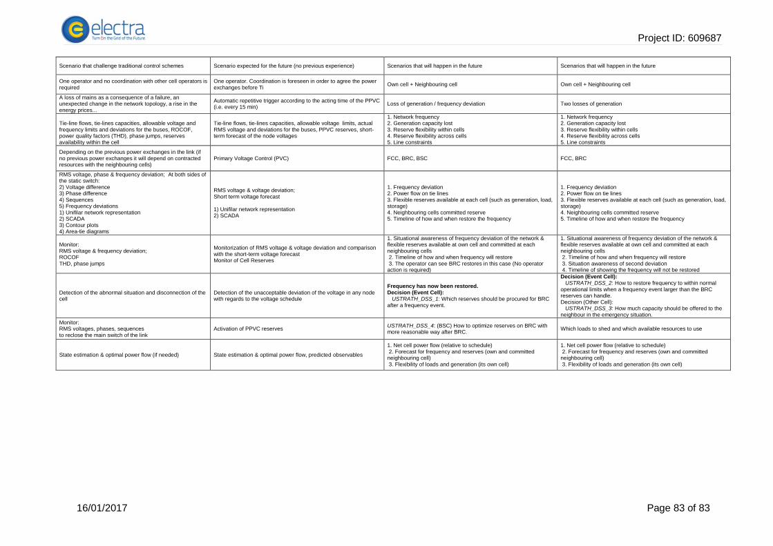
Project ID: 609687
16/01/2017 Page 83 of 83
Scenario that challenge traditional control schemes Scenario expected for the future (no previous experience) Scenarios that will happen in the future Scenarios that will happen in the future
One operator and no coordination with other cell operators is required
One operator. Coordination is foreseen in order to agree the power exchanges before Ti
Own cell + Neighbouring cell Own cell + Neighbouring cell
A loss of mains as a consequence of a failure, an unexpected change in the network topology, a rise in the energy prices...
Automatic repetitive trigger according to the acting time of the PPVC (i.e. every 15 min)
Loss of generation / frequency deviation Two losses of generation
Tie-line flows, tie-lines capacities, allowable voltage and frequency limits and deviations for the buses, ROCOF, power quality factors (THD), phase jumps, reserves availability within the cell
Tie-line flows, tie-lines capacities, allowable voltage limits, actual RMS voltage and deviations for the buses, PPVC reserves, short-term forecast of the node voltages
1. Network frequency 2. Generation capacity lost 3. Reserve flexibility within cells 4. Reserve flexibility across cells 5. Line constraints
1. Network frequency 2. Generation capacity lost 3. Reserve flexibility within cells 4. Reserve flexibility across cells 5. Line constraints
Depending on the previous power exchanges in the link (if no previous power exchanges it will depend on contracted resources with the neighbouring cells)
Primary Voltage Control (PVC) FCC, BRC, BSC FCC, BRC
RMS voltage, phase & frequency deviation; At both sides of the static switch: 2) Voltage difference 3) Phase difference 4) Sequences 5) Frequency deviations 1) Unifilar network representation 2) SCADA 3) Contour plots 4) Area-tie diagrams
RMS voltage & voltage deviation; Short term voltage forecast 1) Unifilar network representation 2) SCADA
1. Frequency deviation 2. Power flow on tie lines 3. Flexible reserves available at each cell (such as generation, load, storage) 4. Neighbouring cells committed reserve 5. Timeline of how and when restore the frequency
1. Frequency deviation 2. Power flow on tie lines 3. Flexible reserves available at each cell (such as generation, load, storage) 4. Neighbouring cells committed reserve 5. Timeline of how and when restore the frequency
Monitor: RMS voltage & frequency deviation; ROCOF THD, phase jumps
Monitorization of RMS voltage & voltage deviation and comparison with the short-term voltage forecast Monitor of Cell Reserves
1. Situational awareness of frequency deviation of the network & flexible reserves available at own cell and committed at each neighbouring cells 2. Timeline of how and when frequency will restore 3. The operator can see BRC restores in this case (No operator action is required)
1. Situational awareness of frequency deviation of the network & flexible reserves available at own cell and committed at each neighbouring cells 2. Timeline of how and when frequency will restore 3. Situation awareness of second deviation 4. Timeline of showing the frequency will not be restored
Detection of the abnormal situation and disconnection of the cell
Detection of the unacceptable deviation of the voltage in any node with regards to the voltage schedule
Frequency has now been restored. Decision (Event Cell): USTRATH_DSS_1: Which reserves should be procured for BRC after a frequency event.
Decision (Event Cell): USTRATH_DSS_2: How to restore frequency to within normal operational limits when a frequency event larger than the BRC reserves can handle. Decision (Other Cell): USTRATH_DSS_3: How much capacity should be offered to the neighbour in the emergency situation.
Monitor: RMS voltages, phases, sequences to reclose the main switch of the link
Activation of PPVC reserves USTRATH_DSS_4: (BSC) How to optimize reserves on BRC with more reasonable way after BRC.
Which loads to shed and which available resources to use
State estimation & optimal power flow (if needed) State estimation & optimal power flow, predicted observables
1. Net cell power flow (relative to schedule) 2. Forecast for frequency and reserves (own and committed neighbouring cell) 3. Flexibility of loads and generation (its own cell)
1. Net cell power flow (relative to schedule) 2. Forecast for frequency and reserves (own and committed neighbouring cell) 3. Flexibility of loads and generation (its own cell)