Demonstration of fault detection and diagnosis … University Institutional Repository Demonstration...

Loughborough UniversityInstitutional Repository

Demonstration of faultdetection and diagnosismethods for air-handlingunits (ASHRAE 1020-RP)

This item was submitted to Loughborough University's Institutional Repositoryby the/an author.

Citation: NORFORD, L.K. ... et al, 2002. Demonstration of fault detectionand diagnosis methods for air-handling units (ASHRAE 1020-RP). HVAC&RResearch, 8 (1), pp. 41-71

Additional Information:

• This is a journal article [ c© American Society of Heating, Refrigeratingand Air-Conditioning Engineers, Inc. (www.ashrae.org)]. Reprinted bypermission from HVAC&R Research, Vol. 8, Part 1. Additional repro-duction, distribution, or transmission in either print or digital form is notpermitted without ASHRAE's prior written permission. It is also availableat: www.ashrae.org/hvacr-research

Metadata Record: https://dspace.lboro.ac.uk/2134/3721

Publisher: c©American Society of Heating, Refrigerating and Air-ConditioningEngineers, Inc.

Please cite the published version.

https://dspace.lboro.ac.uk/2134/3721

This item was submitted to Loughborough’s Institutional Repository (https://dspace.lboro.ac.uk/) by the author and is made available under the

following Creative Commons Licence conditions.

For the full text of this licence, please go to: http://creativecommons.org/licenses/by-nc-nd/2.5/

VOL. 8, NO. 1 HVAC&R RESEARCH JANUARY 2002

41

Demonstration of Fault Detection and Diagnosis Methods for Air-Handling Units

(ASHRAE 1020-RP)

L.K. Norford, Ph.D. J.A. Wright, Ph.D., C.Eng R.A. BuswellMember ASHRAE Member ASHRAE

D. Luo, Ph.D. C.J. Klaassen A. SubyStudent Member ASHRAE Member ASHRAE Member ASHRAE

Results are presented from controlled field tests of two methods for detecting and diagnosingfaults in HVAC equipment. The tests were conducted in a unique research building that featuredtwo air-handling units serving matched sets of unoccupied rooms with adjustable internal loads.Tests were also conducted in the same building on a third air handler serving areas used forinstruction and by building staff. One of the two fault detection and diagnosis (FDD) methodsused first-principles-based models of system components. The data used by this approach wereobtained from sensors typically installed for control purposes. The second method was based onsemiempirical correlations of submetered electrical power with flow rates or process controlsignals.

Faults were introduced into the air-mixing, filter-coil, and fan sections of each of the threeair-handling units. In the matched air-handling units, faults were implemented over three blindtest periods (summer, winter, and spring operating conditions). In each test period, the precisetiming of the implementation of the fault conditions was unknown to the researchers. The faultswere, however, selected from an agreed set of conditions and magnitudes, established for eachseason. This was necessary to ensure that at least some magnitudes of the faults could bedetected by the FDD methods during the limited test period. Six faults were used for a singlesummer test period involving the third air-handling unit. These fault conditions were completelyunknown to the researchers and the test period was truly blind.

The two FDD methods were evaluated on the basis of their sensitivity, robustness, the numberof sensors required, and ease of implementation. Both methods detected nearly all of the faultsin the two matched air-handling units but fewer of the unknown faults in the third air-handlingunit. Fault diagnosis was more difficult than detection. The first-principles-based method mis-diagnosed several faults. The electrical power correlation method demonstrated greater successin diagnosis, although the limited number of faults addressed in the tests contributed to this suc-cess. The first-principles-based models require a larger number of sensors than the electricalpower correlation models, although the latter method requires power meters that are not typi-cally installed. The first-principles-based models require training data for each subsystemmodel to tune the respective parameters so that the model predictions more precisely representthe target system. This is obtained by an open-loop test procedure. The electrical power correla-tion method uses polynomial models generated from data collected from “normal” system oper-ation, under closed-loop control.

Leslie K. Norford is an associate professor at the Massachusetts Institute of Technology, Cambridge, MA. Jonathan A.Wright is a senior lecturer and Richard A. Buswell is a research associate with Loughborough University, Departmentof Civil and Building Engineering, Loughborough, U.K. Dong Luo is a senior engineer with United Technologies Cor-poration. Curtis J. Klaassen is manager of Iowa Energy Center’s Energy Resource Station. Andy Suby is project engi-neer at the Center for Sustainable Environmental Technologies, Iowa State University.

42 HVAC&R RESEARCH

Both methods were found to require further work in three principal areas: to reduce the num-ber of parameters to be identified; to assess the impact of less expensive or fewer sensors; andto further automate their implementation. The first-principles-based models also require furtherwork to improve the robustness of predictions.

INTRODUCTIONIn the last decade, a considerable amount of research has been carried out in the field of fault

detection and diagnosis in HVAC systems. Hyvarinen and Karki (1996) summarized the effortsof an international collaboration [International Energy Agency (IEA) Annex 25] that listed typi-cal faults in heating systems ranging from oil burners to district heating distribution systems;vapor-compression and absorption refrigeration machines; variable air volume (VAV) air-handling units (AHUs); and thermal storage systems. This work also produced a number of faultdetection and diagnosis (FDD) methods:

Innovation approaches• Physical models• Time-series models• State-estimation methods

Parameter-estimation approaches• Methods based on physical models• Characteristic curves• Characteristic parameters

Classification approachesTopological case-based modeling

• Artificial neural networksExpert-system approaches

• Rule-based methods• Associative networks

Qualitative approaches• Formal qualitative approaches• Fuzzy models

Many participants in this effort described their own methods; those of a generic nature or thatfocused on AHUs include Dexter and Benouarets (1996), Haves et al. (1996), Lee et al. (1996a,1996b), Salsbury (1996), Yoshida et al. (1996), and Peitsman and Bakker (1996). These meth-ods were developed and tested with simulations and laboratory test rigs where a high degree ofexperimental control can be applied. Such issues as interfaces with commercially available con-trol systems, identification of the intended users and their needs, and methods for testing andevaluating the performance of FDD systems in systems installed in real buildings were notaddressed. IEA Annex 34 followed Annex 25 and focused on the practical application of FDDtechniques in real buildings (Dexter and Pakanen 2001).

ASHRAE sponsored the research described in this paper as a contribution to the global effortto demonstrate FDD methods in real buildings. This research focused on demonstrating FDDmethods applied to systems installed in real buildings, encompassing the FDD methods, resultsfrom the trials, and the evaluation of the FDD method performance. The three objectives of theresearch were to

1. Demonstrate the operation of FDD methods for HVAC systems in a realistic building envi-ronment

VOLUME 8, NUMBER 1, JANUARY 2002 43

2. Compare the performance of different FDD methods for different types of faults in AHUsand to assess the costs of their implementation

3. Archive and document the test data so they can be used to develop and test other FDDmethods

Each of these objectives carried equal weight and each was largely met. This paper reports thecompleted work with respect to the first two objectives. A more substantial account andarchived data are available in the final report to ASHRAE (Norford et al. 2000).

This research considered VAV AHUs only, although the methods can be applied to other typesof HVAC systems. Both methods were based on a reference-model approach, where measure-ments from the system are compared to model predictions. A significant difference between themodel predictions and the observations indicates that the system has deviated from the expectedoperating condition, which is taken to indicate the presence of a fault. The first-principles-basedapproach modeled the subsystem components and used fluid (air/water) quantity and propertymeasurements and control-signal observations. The detection of faults focused on the effect of thefault condition on the output of the system process. The electrical power correlation methodrelated electrical power measurements to fluid quantity and property measurements and control-signal observations; changes in the correlations were considered to be faults.

A description is given of the test building and the HVAC systems. The faults, their implemen-tation and the FDD methods are described. The results from the four test periods are presented.The methods are evaluated on the basis of the accuracy, calibration, and cost of the required sen-sors; the ease of implementation of the methods, including selection and estimation of the modelparameters and thresholds; the sensitivity and robustness of the methods in fault detection; andtheir success in fault diagnosis.

BUILDING, SYSTEMS, AND FAULTSThe fault-test program was conducted in a unique building that combined laboratory testing

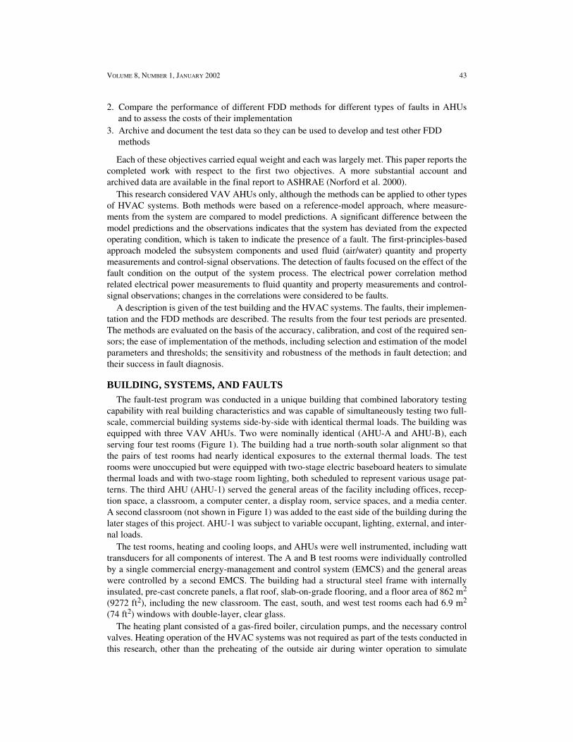
capability with real building characteristics and was capable of simultaneously testing two full-scale, commercial building systems side-by-side with identical thermal loads. The building wasequipped with three VAV AHUs. Two were nominally identical (AHU-A and AHU-B), eachserving four test rooms (Figure 1). The building had a true north-south solar alignment so thatthe pairs of test rooms had nearly identical exposures to the external thermal loads. The testrooms were unoccupied but were equipped with two-stage electric baseboard heaters to simulatethermal loads and with two-stage room lighting, both scheduled to represent various usage pat-terns. The third AHU (AHU-1) served the general areas of the facility including offices, recep-tion space, a classroom, a computer center, a display room, service spaces, and a media center.A second classroom (not shown in Figure 1) was added to the east side of the building during thelater stages of this project. AHU-1 was subject to variable occupant, lighting, external, and inter-nal loads.

The test rooms, heating and cooling loops, and AHUs were well instrumented, including watttransducers for all components of interest. The A and B test rooms were individually controlledby a single commercial energy-management and control system (EMCS) and the general areaswere controlled by a second EMCS. The building had a structural steel frame with internallyinsulated, pre-cast concrete panels, a flat roof, slab-on-grade flooring, and a floor area of 862 m2

(9272 ft2), including the new classroom. The east, south, and west test rooms each had 6.9 m2

(74 ft2) windows with double-layer, clear glass.The heating plant consisted of a gas-fired boiler, circulation pumps, and the necessary control

valves. Heating operation of the HVAC systems was not required as part of the tests conducted inthis research, other than the preheating of the outside air during winter operation to simulate

44 HVAC&R RESEARCH

higher outside temperatures and force the HVAC systems into economizer mode. The coolingplant (Figure 2), consisted of a nominal 35 kWthermal (10 ton) two-stage, reciprocating air-cooledchiller; a 525 kWhthermal (149 ton ⋅h) thermal energy storage (TES) unit that was isolated from thecooling system for this research; and chilled water supplied by a central facility, with pumps,valves, and piping to circulate chilled water through the HVAC components.

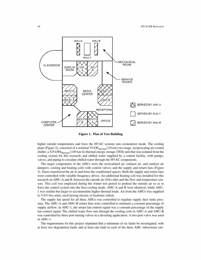
The major components of the AHUs were the recirculated air, exhaust air, and outdoor airdampers; cooling and heating coils with control valves; and the supply and return fans (Figure3). Ducts transferred the air to and from the conditioned spaces. Both the supply and return fanswere controlled with variable-frequency drives. An additional heating coil was installed for thisresearch on AHU-A and B, between the outside air (OA) inlet and the flow and temperature sen-sors. This coil was employed during the winter test period to preheat the outside air so as toforce the control system into the free-cooling mode. AHU-A and B were identical, while AHU-1 was similar but larger to accommodate higher thermal loads. Air from the AHUs was suppliedto VAV box units, each having electric or hydronic reheat.

The supply fan speed for all three AHUs was controlled to regulate supply duct static pres-sure. The AHU-A and AHU-B return fans were controlled to maintain a constant percentage ofsupply airflow; in AHU-1, the return fan control signal was a constant percentage of the supplyfan control signal. The chilled water flow rate through the cooling coils in AHU-A and AHU-Bwas controlled by three-port mixing valves in a diverting application. A two-port valve was usedin AHU-1.

The requirements for this project stipulated that a minimum of six faults be investigated, withat least two degradation faults and at least one fault in each of the three AHU subsystems (air-

Figure 1. Plan of Test Building


Figure 2. Chilled Water Flow Circuit in Test Building

46 HVAC&R RESEARCH

mixing, filter-coil, and fan). Table 1 shows the seven selected faults and their method of imple-mentation for AHU-A and AHU-B. Although faults implemented through software or easily dis-connected hardware (such as actuator linkages) were readily introduced, others requiredsubstantial system modification, including the installation of bypass piping and additional valves.

It was necessary, in the context of the research, to ensure that both FDD methods were (inprinciple) capable of detecting all of the faults. Clearly, little would be learned from a series ofnull results. This criterion eliminated some faults, such as temperature sensor faults that theelectrical power method would have difficulty detecting. This criterion was relaxed for testswith AHU-1, discussed later.

Table 2 indicates that each fault was implemented in at least two of the three test periods heldduring summer, winter, and spring seasons. Each test period consisted of a week of controlledtests, when the research staff of the test building introduced faults known to the investigators, ashort analysis period, and a week of blind tests. For each blind test period, the list of possiblefaults was made known, but not the order of implementation or whether they were implementedat all. The lists for each season excluded faults that would not be seen in that season. For exam-ple, the recirculation damper would normally be fully open in hot weather (minimum outsideair) and a damper leak could not be detected. Abrupt faults were typically implemented over a24 h period while most degradation faults required three days, one for each of three stages. Thethree stages of the drifting pressure sensor fault were introduced over a single day.

Fault magnitudes were established during an initial period when the FDD methods were com-missioned and the procedures for introducing faults and the HVAC systems were developed.The magnitudes of the degradation faults were selected such that it was anticipated that the twoFDD methods would be able to detect the largest level, should be able to detect the middle level

Figure 3. Air-Handling Unit in Test Building


and could possibly detect the lowest level. Fault magnitudes were consistent in each of the threetest periods. Constant-magnitude faults provided a firmer basis for evaluating the FDD methodsand were implemented with less difficulty than the variable-magnitude faults (a change of faultmagnitude over different occurrences at different times) that would likely occur in practice.HVAC system commissioning consisted primarily of sensor calibration and establishing stan-dard system operating configurations; the latter was required because the research facilityaltered the systems between test periods to meet the needs of other research programs. The con-figuration setup, which proved to be a major task for the test-building staff, encompassed fancontrol algorithms, isolation of the thermal storage tank (which provided a thermal capacitancethat interfered with analysis of chiller cycling periods), and operating schedules for both HVACequipment and false loads in the test rooms.

A more realistic set of blind tests was conducted with AHU-1, the air handler serving areas ofthe building occupied by research staff and classroom visitors. Four days of normal operationfor training FDD methods and 17 days for fault introduction were included in a summer periodof about six weeks. Building loads were not controlled and four of the six faults (listed in Table3) had not been implemented in AHU-A and AHU-B and were completely unknown to theinvestigators. This test period was considerably longer than each of the three test periods on thematched AHUs, and increased the possibility of naturally occurring faults.

Two of the faults in this program produced signatures different from the naturally occurringfaults they were intended to represent: the leaky cooling coil valve and the coil capacity fault.The leaking valve was implemented with a specially installed bypass valve that generated thesame thermal effect as a leakage past a closed control port, but changed the flow resistance. Thecoil capacity fault mimicked the impact of water-side fouling on heat transfer across the coolingcoil to some extent. A simpler alternative to replacing the existing coil with an older coil withtubes fouled with calcium carbonate was to close a valve in the inlet leg to the coil, thus increas-

Table 1. Method of Implementation of Faults

Fault Type Implementation

Air-Mixing SectionStuck-closed recirculation damper

Abrupt Application of a control voltage from an independent source to maintain the damper in the closed position.

Leaking recirculation damper

Degradation Removal of the recirculation damper seals, with one seal removed for the first fault stage, two for the second, and all seals for the third stage.

Filter-Coil SectionLeaking cooling coil valve Degradation Manual opening of a coil bypass valve.Reduced coil capacity (water-side)

Degradation Manual throttling of the cooling coil balancing valve, to 70%, 42%, and 27% of the maximum coil flow of 1.7 L/s (27.5 gpm) for the three fault stages.

Fan Drifting pressure sensor Degradation Introduction of a controlled leak in the pneumatic signal

tube from the supply duct static pressure sensor to the transducer, to a maximum reduction of 225 Pa (0.9 in. of water).

Unstable supply fan controller

Abrupt Introduction of alternative gains for the PID controller that adjusts fan speed to regulate static pressure.

Slipping supply fan belt Degradation Adjustment of fan belt tension to reduce maximum fan speed by 15% at 100% control signal for the first stage and 20% for the second stage. The third stage had an extremely loose belt with variable fan speed.

48 HVAC&R RESEARCH

ing the resistance to water flow. This change in flow resistance became the basis for its detectionwith the electrical power FDD method.

Daily data sets for normal and faulty operation were assembled by the test-building staff fromlogs made by the EMCSs and were posted for electronic transfer to the investigators’ home sites.

DETECTION AND DIAGNOSIS

The two fault detection methods compare the differences between the observed system behav-ior and a reference model of the system operation. The approaches differ significantly in how thefault effects are observed. The first-principles-based method considers the performance of themonitored system in terms of the system output useful to the air-conditioning process. In this case,the model predicts the temperature of the air or the static air pressure at the outlet of the compo-nent. A fault can be described in these terms as a degradation in the expected system performance.

Table 2. Faults Introduced into AHU-A and AHU-B During Three Blind Test Periods

Fault Summer Winter Spring

Air-Mixing SectionStuck-closed recirculation damper X XLeaking recirculation damper X X

Filter-Coil SectionLeaking cooling coil valve X XReduced coil capacity (water-side) X X

Fan Drifting pressure sensor X X XUnstable supply fan controller X X XSlipping supply fan belt X X

Table 3. Faults Introduced into AHU-1 During Blind Test Period andTheir Method of Implementation

Fault Type Implementation

Air-Mixing SectionStuck-closed recirculation damper

Abrupt Application of a control voltage from an independent source to maintain the damper in the closed position for about 24 h

Stuck-open outside air damper

Abrupt Application of a control voltage from an independent source to maintain the damper in the open position for 24 h

Filter-Coil SectionLeaking heating coil valve Abrupt Adjustment of output voltage to the heating coil valve,

causing it to unseat and leak for about 29 hFouled cooling coil Degradation Blockage of the cooling coil with a curtain drawn from

the bottom to cover 25%, 50%, and 75% of the 61 cm (24 in.) coil in the three fault stages

Fan Drifting pressure sensor Degradation Introduction of a controlled leak in the pneumatic signal

tube from the supply duct static pressure sensor to the transducer, with pressure reduced by 50, 100, and 150 Pa in the three fault stages (0.2, 0.4, and 0.6 in. of water) and each stage implemented for at least 6 h

Loss of control of supply fan

Abrupt Supply fan VFD isolated from EMCS and operated at a constant speed for about 23 h


The electrical power correlation method uses models derived from the system characteristics thatrelate electrical load to certain variables. This method predicts the expected power consumption.In this case a fault can be described as a change in the expected system energy consumption.

Both methods can take advantage of certain fault characteristics and not of others. The first-principles-based approach will always detect a degradation in the performance of the thermo-fluid system (as long as it is significant), regardless of the cause. The electrical power correlationmethod will not detect a fault that affects performance but has no effect on the electrical load. Itis, however, predisposed to generating an operating cost associated with the faulty behavior and itcan, in principle, detect faults associated with motors and drive trains that the first-principles-based approach cannot detect.

Fault diagnosis is also based on the information available to each method. The sensors requiredto implement FDD are one principal difference between the two methods. The first-principles-based approach uses measurements typically installed for control (temperatures, humidities, flowrates, etc.). One disadvantage with this approach is that in general terms there can be less controlover the quality of these measurements in any given installation. The electrical power correlationmethod uses sensors over and above those normally installed, but these are more focused for theintended application and are not as susceptible to poor installation and maintenance.

First-Principles-Based Models with Thermo-Fluid MeasurementsFirst-principles-based (or analytical) models can be used as a reference for the “correct” or

expected operation of a HVAC system. The approach used in this research relied on the sensorstypically installed in most VAV systems for control. Three subsystem models [described morefully in Norford et al. (2000)] were used to implement the FDD scheme: a fan/duct model of theair system, an economizer model, and a model of the coiling-coil subsystem. Figure 4 demon-strates the modeling arrangement. The black dots indicate where the comparisons to the obser-vations from the real system were made, and hence where the fault detection for each subsystemwas focused. Simple, steady-state simulations of the subsystems are formed by the models,which are based on the following principles:

• The fan/duct model is based on the fan laws and simple quadratic expressions for the changein system resistance and predicts the supply air static pressure.

• The economizer model is based on the analytical representation of the mixed-air condition asa function of damper position and the inlet temperatures and humidities. The model alsoincludes an actuator model.

• The cooling coil model is based on the SHR method effectiveness-NTU heat and mass trans-fer calculation method [similar to the ASHRAE 3-line method; a review of both methods isgiven by Stephan (1994)]. The subsystem model also includes fan temperature rise and mod-els for the control valve and the actuator.

• The fan-temperature-rise model is a simple addition to the air temperature, linearly dependenton the fan-control signal.

• The valve model is based on a first-principles analysis of the water-circuit resistance withrespect to the control valve. The model predicts the mass flow rate of water through the coil, atypically unmeasured variable.

• The actuator model is an analytical representation of the movement of the actuator inresponse to a control signal. This models the dead-bands at either end of the operating rangeand any hysteresis (slack in the linkage) that may be present in the system.

The models have parameters for which values must be estimated for a specific system. Theparameters are designed, as far as possible, to represent some tangible system characteristic andgive greater precision in prediction. An example of this is the actuator “low activation point”

50 HVAC&R RESEARCH

parameter, which describes the value of the control signal required before the valve stem startsto move as it is opened from the closed position (i.e., dead-band). Some of the model parameterscan be obtained from design information or inspection of the installed system. The face area andnumber of rows and circuits in the cooling coil are examples. The remaining parameters areidentified simultaneously for each subsystem model. The model parameters are estimated byapplying a nonlinear optimization technique, minimizing the model prediction errors in a least-squares sense. The data used for this procedure were generated by applying a sequence of open-loop “steps” in the inputs to capture the system characteristics when the system was in a normal(fault-free) condition.

With the system models characterized, model predictions can be applied to the observations to gen-erate the “prediction error” (demonstrated in the top halves of Figures 5 and 6). The models only applyto observations that are close to steady state and a steady-state filter removes data containing tran-sients. A lack of steady-state data was used to identify the presence of oscillatory, or unstable, control.

Figure 4. First-Principles-Based Model Functionality


Some prediction error will always exist due to uncertainties in the measurements and unmod-eled system disturbances. Statistically based thresholds are applied to the prediction error, suchthat a certain magnitude of error is required before triggering an alarm.

Once an alarm has been identified, the cause is diagnosed. Two methods were investigated inthis work, fault diagnosis by (1) expert rules and by (2) recursive parameter estimation. Theschemes are shown in Figures 5 and 6, respectively. Figure 5 shows that the “innovations” (themagnitude of the prediction error over and above the thresholds) were split into three “bins.”

Figure 5. Method for Fault Detection and Fault Diagnosis Using Expert Rules

52 HVAC&R RESEARCH

The bins contain the average magnitudes of the innovations, exponentially weighted with age.Each bin represents a portion of the operating space of the monitored process. Crisp expert ruleswere then applied to the average values in these bins to determine the cause of the fault.

In the recursive parameter estimation scheme, some of the parameters are designed to repre-sent the effects of the faults on the system output. These parameters are recursively re-estimatedto track the developing fault. The algorithm minimizes the prediction error and uses the sensitiv-

Figure 6. Method for Fault Diagnosis by Recursive Parameter Estimation


ity coefficients of the fault parameters with respect to the model output to drive the estimationprocedure (Salsbury 1996). As the fault develops, the current fault parameter values implicitlydescribe the state of the system and hence, diagnose the state of the system.

Gray-Box Correlations with Electrical Measurements

The electrical power correlation FDD method produced prediction errors in electrical power.The method also made use of statistically derived confidence intervals for predictions of perfor-mance under normal operation. The method is a semiempirical approach that correlates mea-sured fan or pump power with such exogenous variables as airflow, motor speed control signalsand actuator position control signals. Power correlations were third-order polynomials; confi-dence intervals reflected the influence of disturbances during training periods, such as those dueto normal variation in damper positions. Oscillatory power data, indicative of unstable local-control loops, were detected via a calculation of signal variance over a sliding window of datapoints; this calculation effectively acted as a steady-state filter by excluding oscillatory datafrom comparison with power correlations established during the training phase.

Analysis of chiller power (associated with the economizer and cooling coil valve leakagefaults) was more difficult than for fans (air system faults) and pumps (cooling coil undercapacityfault), for two reasons. First, the chiller in the test building was a two-stage reciprocating unitwith discrete power levels (0, 5, and 10 kW). In principle, it was possible to time-average thepower to obtain a continuous power variable suitable for the same sort of power correlationsused for fans and pumps. In practice, the cycling frequency was often long (i.e., on the order of30 minutes), making it impossible to calculate a short-term power average needed for reasonablecorrelation with driving variables. Second, chiller power was strongly influenced by environ-mental conditions (expressed by dry-bulb and wet-bulb temperatures and solar radiation) and bybuilding internal loads. These variables are not all easily measured. Even those that are directlyand simply measurable require sensors that have a cost associated with them and are subject toerrors. It is necessary to either include these influences in a model of chiller power or excludethem and limit the analysis of chiller power to narrow and known operating conditions.

The FDD method developed and applied in the test building assessed chiller cycling periodsunder two low-load conditions where it was, in principle, possible to discern a change in chillerloading due to damper and valve leaks.

The method relied heavily on one-minute-average data from installed power transducers toassess the benefits of such data and set the stage for a future cost-benefit analysis. A detailed dis-cussion of the method is presented in a companion paper (Shaw et al. 2002), which includesexamples of power correlations, detection of chiller cycling, and analysis of power oscillations.

Table 4 summarizes the types of electrical power analyses used in this method, along with alist of possible faults that each analysis can detect. The list of faults is not exhaustive but is longenough to indicate the difficulties in distinguishing a particular fault from other possible causesof the same deviation between predicted and measured electrical power.

Expert rules were used for limited fault diagnosis. Table 4 indicates how rules can distinguish aslipping fan belt from a fault caused by a change in flow resistance: the former leads to powermeasurements that differ from the predicted value for a given motor speed while the latter doesnot. (For the slipping fan belt, the reduction in power due to reduced airflow was a stronger effectthan an increase in thermal dissipation from the fan belt itself, which became quite hot when slip-ping.) Although careful analysis of fan curves indicates that this statement is not entirely true, theimpact of a change in duct pressure on the power-speed correlation is sufficiently minimal to beof no concern. As a second example, the leaky recirculation damper or cooling coil valve willaffect chiller power but not fan power for a given airflow.

54 HVAC&R RESEARCH

Ideally, a given power signature would be associated with nonoverlapping lists of faults, pro-viding a high level of “orthogonality” useful for fault diagnosis. As can be seen in Table 4, thisideal was not achieved. Errors in power transducers and changes in fan or motor performancewill affect both types of fan power correlations. In the blind tests, it was possible in some casesto distinguish faults associated with a given power correlation by limiting the analysis to a smallrange of the correlation or to a narrow band of another variable:

• The stuck-closed recirculation damper could be distinguished from the pressure sensor offsetin the test building via analysis of power at low airflows. The impact of the stuck-closed recir-culation damper fault was exacerbated in the early evening, when the air handlers were stillrunning but, in cold or hot weather, the outdoor air damper was fully closed. The supply fanthen drew air across two closed dampers. There is substantial variation across buildings incontrol strategies at the beginning and end of the working day and it is difficult to generalizesuch an approach. Even in the test building, this strategy could not be generalized to AHU-1,which operated continuously.

• The leaky cooling coil valve and the leaky recirculation damper could be distinguished withthe help of measurements of the valve position control signal and outdoor temperature (Shawet al. 2002).

This approach to fault diagnosis, while unable to distinguish a large set of possible faults, waseasily implemented in rules. For the blind tests, where the number of possible faults was limited,

Table 4. Nonexhaustive Listing of Faults Associated with a GivenElectrical Power Signature

Type ofElectrical Power Analysis

Possible Faults Causing a Deviation Between Predicted and Measured Electrical Power

Polynomial correlation of supply fan power with supply airflow

Change in airflow resistance, possibly due to stuck air-handler dampers or fouling of heating or cooling coils

Static pressure sensor error (affects portion of fan power due to static pressure)

Flow sensor errorPower transducer errorChange in fan efficiency, caused by change in blade type or

pitch, or use of VFD in lieu of inlet vanesChange in motor efficiency

Polynomial correlation of supply fan power with supply fan speed control signal

Slipping fan beltDisconnected control loop (fan speed differs from control

signal)Power transducer errorChange in fan efficiencyChange in motor efficiency

Polynomial correlation of chilled water pump power with cooling coil control valve position control signal

Change in water flow resistance, possibly due to constricted cooling coil tubes or piping

Disconnected control loopPower transducer errorChange in pump efficiencyChange in motor efficiency

Detection of change in cycling frequency for two-stage reciprocating chiller

Leaky cooling coil valveLeaky recirculation damper

Detection of power oscillations Unstable local-loop controller


one rule was “if the electrical power exceeds the confidence interval and the airflow is less thana threshold, then the fault is a stuck-closed recirculation damper.” More generally, the “if-then”statement could be modified to include a larger list of possible causes of the detected fault.

RESULTSThe results from the FDD trials on AHU-A/B and AHU-1 are shown in Tables 5 through 8.

The original intent of the first-principles-based approach was to not use the mixed-air tempera-ture sensor because this is not commonly available. The predictions of the mixed-air humidityratio and temperature by the economizer model were used as inputs to the cooling coil model.The magnitudes of prediction errors associated with normal operation in the mixing box andcooling coil (due to the influence of unmodeled disturbances) led to a reduction in sensitivity tofault detection. There was also a significant reduction in the isolation of the cause of faults(faults possibly being in one of two subsystems), which led to ambiguous diagnoses. The modelparameters were re-estimated using the mixed-air temperature measurement and the summertests were rerun with the addition of this measurement. The analyses for the other season werecarried out using the same models.

Table 5 describes the first blind test period, conducted in summer conditions on AHU-A andAHU-B. Tables 6 and 7 describe the winter and spring blind test periods. The tests on AHU-1are summarized in Table 8; for these tests the first-principles-based FDD approach gave a singlediagnosis through application of the RPE method and expert rules.

For both the first-principles-based models and the electrical power correlation method, theresults are discussed first for AHU-A and AHU-B and then AHU-1. Where individual faults arehighlighted, the order is the same as that presented in Tables 2 and 3.

First-Principles Models with Thermo-Fluid MeasurementsIn general, the first-principles-model-based FDD method proved to be effective in the detec-

tion of the faults implemented on AHU-A and B. All faults were detected in each season theywere implemented, with the exception of the leaking recirculation damper and leaking coolingcoil valve. Diagnosis was less reliable, in that no single method of diagnosis (expert rules orrecursive parameter estimation) was able to provide a diagnosis for all fault conditions.

A leaking recirculation damper can be expected to produce small differences between theexpected and observed mixed-air temperature. This is, however, a function of the temperaturedifference between the ambient and return air streams (when these temperatures are equal, nofaults can be detected using temperature measurements) and the size of the leakage. In order todetect these changes, the model of the economizer must be quite precise in its prediction of themixed-air temperature. The principal factors affecting the precision of the model were

• Stratification at the locations of the temperature sensors (return and mixed), which affects thecalibration of the model parameters and subsequent calculations of prediction error.

• Localized offsets caused by differences between the measured ambient-air temperature andthe temperature of the ambient air entering the inlet duct, some distance away. The effect wassimilar to the above point.

• Unmodeled effects, of which there were two primary sources:• The pressure/resistance characteristics for the fan/duct system were not constant as

a result of the fan control strategy (return fan runs at a fixed percentage of the sup-ply air volumetric flow rate). This meant that at different fan speeds, different pro-portions of the ambient air and return air were mixed for a given damper position.Prediction errors are generated because the model assumes that these proportionsare unchanging (i.e., that the system is well balanced).

56 HVAC&R RESEARCH

• At certain conditions, the fan/duct system imbalance also caused ambient air toflow in through the exhaust grille, resulting in a higher proportion of the ambientair in the mixed air than expected by the model. This problem was exacerbated inthe system under investigation because of the increased resistance to airflowthrough the ambient air inlet duct due to the installation of the preheat coil.

These problems can be considered to be system faults and not problems with the FDDmethod. The last point highlights the disadvantages of an analytical modeling approach appliedto observations of the result of the process, rather than modeling the process itself. Given a moredetailed fan/duct system model, it may be possible to predict the airflow rates within the system(within a tolerable degree of uncertainty), which would eliminate the need for the mixing boxmodel as presented in this work.

Table 5. Detection and Diagnosis of Faults During Summer Blind Test Period for AHU-A and AHU-B

TestDay

AHU

Physical Models

Electrical PowerModels

Detectfrom

Innovations

Diagnose from

ExpertRules

Diagnose from

Recursive Parameter EstimationA B Detect Diagnose

1 Slipping fan belt (Stage 1)

No — — Yes Yes

Reduced cooling coil capacity(Stage 1)

Yes Yes No Yes Yes


No — — Yes Yes


Yes Yes No Yes Yes


Yes No Yes Yes Yes


Yes Yes No Yes Yes

4 No fault No fault — — No fault —

Unstable pressure control

Yes* — — Yes Yes

5 Unstable pressure control

Yes* — — Yes Yes

No fault No fault — — No fault —

6 Static-pressure sensor offset (Stages 1-3)

Yes No Yes Yes Yes

Stuck-closed recirculation damper

Yes No Yes Yes Yes

7 Stuck-closed recirculation damper

Yes Yes Yes Yes Yes

Slipping fan belt (Stage 1)

No — — No —

*The unstable pressure controller was detected via the steady-state filter, which indicated that the measured pressure was in a dynamicstate for a prolonged period. No detection or diagnosis method was applied, because the measurements did not pass the filter.


Estimating the parameters for the economizer model means that either the system has to be bal-anced correctly or the training data (ideally) need to encompass the complete range of expectedairflow/resistance characteristics. If the model does not describe its output in these terms, thenrobustness comes through increased uncertainty in the model output (wider confidence limits orthresholds) and reduced sensitivity in fault detection. Practically, the model training data have tobe collected at one or two airflow rates. An improvement would be to retune the thresholds asnew regions of operation are encountered, to maintain maximum sensitivity.

Table 6. Detection and Diagnosis of Faults During Winter Blind Test Period forAHU-A and AHU-B

TestDay

AHU

Physical Models

Electrical PowerModels

Detectfrom

Innovations

Diagnose from

ExpertRules

Diagnose from

Recursive Parameter EstimationA B Detect Diagnose

1 No fault No fault — — No fault —

Stuck-closed recirculation damper

Yes1 No Yes2 Yes Yes

2 Leaking cooling coil valve(Stages 1-3)

No — — Yes Yes


No — — No —

3 Leaking recirculation damper(Stage 1)

No — — Yes Yes


No — — No —

4 Leaking recirculation damper(Stage 2)

No — — Yes Yes


Yes Yes3 Yes Yes Yes

5 Leaking recirculation damper (Stage 3)

No — — Yes Yes

Static pressure sensor offset (Stages 1- 3)

Yes Yes Yes Yes Yes

6 Static pressure sensor offset (Stages 1- 3)

Yes Yes4 Yes5 Yes Yes

Unstable pressure control

Yes Yes Yes Yes Yes

7 Unstable pressure control

Yes6 — — Yes Yes

No fault No fault — — No fault —1Alternative diagnosis of static pressure sensor drift.2Alternative diagnosis of slipping fan belt.3Alternative diagnosis of unknown mixing box fault.4Alternative diagnoses of excessive control dynamics and excessive outside air (due to flow of outdoor air into theexhaust damper, an actual—not artificial—system fault).5Alternative diagnosis of slipping fan belt.6The unstable pressure controller was detected via the steady-state filter, which indicated that the measured pressure wasin a dynamic state for a prolonged period.

58 HVAC&R RESEARCH

Tab

le 7

.D

etec

tion

and

Dia

gnos

is o

f F

ault

s D

urin

g Sp

ring

Blin

d T

est

Per

iod

for

AH

U-A

and

AH

U-B

Tes

tD

ay

AH

U

Phy

sica

l Mod

els

Ele

ctri

cal P

ower

Mod

els

Det

ect

from

In

nova

tion

s D

iagn

ose

from

E

xper

t R

ules

Dia

gnos

e fr

om

Rec

ursi

ve P

aram

eter

E

stim

atio

nA

BD

etec

tD

iagn

ose

1S

tatic

pre

ssur

e se

nsor

of

fset

(St

ages

1-3

)Y

esN

o (u

nkno

wn

faul

t)Y

esY

esY

es

Lea

king

coo

ling

coil

valv

e (S

tage

1)

No

——

Yes

Yes

2U

nsta

ble

pres

sure

co

ntro

l1N

o fa

ult2

—

—N

o fa

ult2

—

Lea

king

coo

ling

coil

valv

e (S

tage

2)

Yes

Yes

No3

Yes

Yes

3N

orm

al o

pera

tion

No

faul

t—

—N

o fa

ult

—

Lea

king

coo

ling

coil

valv

e (S

tage

3)

Yes

Y

esY

es—

4R

educ

ed c

ooli

ng c

oil

capa

city

(S

tage

1)

Yes

No4

No5

Yes

Yes

Nor

mal

ope

rati

onY

esN

o4—

No

faul

t—

5R

educ

ed c

ooli

ng c

oil

capa

city

(S

tage

2)

No

—N

o6N

o—

Lea

king

rec

ircu

latio

n da

mpe

r (S

tage

1)

No

——

No

—

6R

educ

ed c

ooli

ng c

oil

capa

city

(S

tage

3)

Yes

Yes

Yes

7 Y

esY

es

Lea

king

rec

ircu

latio

n da

mpe

r (S

tage

2)

No

—N

o6N

o—

7U

nsta

ble

pres

sure

co

ntro

l1Y

esN

o4,8

No

8,9

Yes

Yes

Lea

king

rec

ircu

latio

n da

mpe

r (S

tage

3)

Yes

Yes

No6

No

—

8U

nsta

ble

pres

sure

co

ntro

lY

es10

——

Yes

Yes

Lea

king

rec

ircu

latio

n da

mpe

r (S

tage

3)

Yes

No11

No6

No

—1 I

mpl

emen

tati

on o

f un

stab

le p

ress

ure

cont

rol

was

con

side

red

by t

est

impl

emen

ters

not

to

have

take

n ef

fect

.2 A

ltho

ugh

the

day

was

lab

eled

as

norm

al b

y th

e ph

ysic

al m

odel

and

ele

ctri

cal

pow

er F

DD

met

h-od

s, p

erio

ds o

f co

ntro

l ins

tabi

lity

wer

e de

tect

ed b

y bo

th m

etho

ds.

3 Dia

gnos

ed a

s in

crea

sed

coil

cap

acit

y (d

isch

arge

-air

tem

pera

ture

low

er t

han

pred

icte

d) o

r an

unkn

own

faul

t. A

n in

crea

se i

n co

il c

apac

ity

wou

ld n

ot r

epre

sent

a d

egra

dati

on f

ault

but

cou

ldin

dica

te th

at th

e co

olin

g co

il h

ad b

een

clea

ned

afte

r th

e m

odel

cal

ibra

tion

per

iod.

4 Dia

gnos

ed a

s a

leak

ing

cool

ing

coil

val

ve.

5 Dia

gnos

ed a

s in

crea

sed

coil

cap

acit

y.

6 Dia

gnos

ed a

s an

unk

now

n fa

ult i

n th

e m

ixin

g bo

x.7 A

lter

nati

ve d

iagn

osis

as

an u

nkno

wn

faul

t in

the

mix

ing

box.

8 The

phy

sica

l mod

el F

DD

met

hod

dete

cted

bri

ef p

erio

ds o

f un

stab

le c

ontr

ol.

9 Dia

gnos

ed a

s in

crea

sed

coil

cap

acit

y.10

The

uns

tabl

e pr

essu

re c

ontr

olle

r w

as d

etec

ted

via

the

stea

dy-s

tate

fil

ter,

whi

chin

dica

ted

that

the

mea

sure

d pr

essu

re w

as i

n a

dyna

mic

sta

te f

or a

pro

long

edpe

riod

. 11

Dia

gnos

ed a

s an

unk

now

n fa

ult.


Tab

le 8

.D

etec

tion

and

Dia

gnos

is o

f F

ault

s fo

r A

HU

-1 B

lind

Tes

t P

erio

d

Tes

t D

ayF

ault

Phy

sica

l Mod

els

Ele

ctri

cal P

ower

Mod

els

Det

ect

from

Inno

vati

ons

Dia

gnos

e fr

om E

xper

t R

ules

and

Rec

ursi

ve P

aram

eter

Est

imat

ion

Det

ect

Dia

gnos

e

July

12N

o fa

ult

Fal

se a

larm

Coi

l und

erca

paci

tyN

o fa

ult

—14

No

faul

tF

alse

ala

rmFa

lse

alar

ms

from

sup

ply

air a

nd c

oolin

g co

il m

odel

s; d

esig

n fa

ult

from

mix

ing

box

mod

el1

No

faul

t—

16N

o fa

ult

Fal

se a

larm

Fals

e al

arm

fro

m c

oolin

g co

il m

odel

2N

o fa

ult

—17

No

faul

tF

alse

ala

rmFa

lse

alar

m f

rom

coo

ling

coil

mod

el2

No

faul

t—

27A

bort

ed f

ault

No

faul

t

No

faul

t28

Stat

ic p

ress

ure

sens

or o

ffse

t (St

ages

1-2

)Y

esY

esY

esY

es29

Stat

ic p

ress

ure

sens

or o

ffse

t (St

ages

2-3

)Y

esY

esY

esY

es30

Stuc

k ou

tdoo

r ai

r da

mpe

rY

es3

Inco

nclu

sive

dia

gnos

is f

rom

mix

ing

box

mod

elN

o—

31St

uck

outd

oor

air

dam

per

No

—N

o—

Aug

ust

1N

orm

al o

pera

tion

No

faul

t—

No

faul

t—

9C

oolin

g co

il ai

r-si

de f

ouli

ng (

Stag

e 1)

Yes

4Fa

lse

alar

m f

rom

coo

ling

coil

mod

el2

No

—10

Coo

ling

coil

air-

side

fou

ling

(St

age

2)Y

es4

Fals

e al

arm

fro

m c

oolin

g co

il m

odel

2N

o—

10-1

1C

oolin

g co

il ai

r-si

de f

ouli

ng (

Stag

e 3)

Yes

4Fa

lse

alar

m f

rom

coo

ling

coil

mod

el2

No

—11

-12

Lea

king

hea

ting

coil

Yes

5Fa

lse

alar

m f

rom

sup

ply

air

mod

el; c

oolin

g co

il c

apac

ity f

ault

No

—13

Stuc

k-cl

osed

rec

ircu

lati

on d

ampe

rY

es5

Yes

—co

rrec

t dia

gnos

is f

rom

the

supp

ly a

ir m

odel

; a f

alse

ala

rm

from

coo

ling

coil

mod

el2

Yes

No

14, 1

5, 1

6N

orm

al o

pera

tion

No

faul

t—

No

faul

t—

17L

oss

of s

uppl

y fa

n co

ntro

l, ab

orte

d af

ter

2h

Yes

No

Yes

No

18L

oss

of s

uppl

y fa

n co

ntro

lN

o—

No

—19

Nor

mal

ope

rati

onN

o fa

ult

—N

o fa

ult

—1 A

fau

lt w

as d

etec

ted

from

inno

vati

ons

in e

ach

of th

e th

ree

mod

els:

sup

ply

air,

mix

ing

box,

and

coo

l-in

g co

il. T

he d

iagn

osis

fro

m th

e su

pply

air

mod

el w

as a

fal

se a

larm

due

to a

poo

r re

pres

enta

tion

of

the

air

dist

ribu

tion

syst

em.

The

dia

gnos

is f

rom

the

mix

ing

box

mod

el w

as a

des

ign

faul

t be

caus

e th

ere

turn

fan

con

trol

for

AH

U-1

, a f

ixed

per

cent

age

of th

e su

pply

fan

spe

ed, i

nflu

ence

d th

e pr

opor

tion

ofou

tsid

e ai

r in

the

supp

ly a

ir. T

he d

iagn

osis

fro

m th

e co

olin

g co

il m

odel

was

a f

alse

ala

rm b

ecau

se th

epr

edic

tion

of

mix

ed a

ir h

umid

ity

need

ed i

n th

e m

odel

was

inf

luen

ced

by t

he r

etur

n fa

n co

ntro

l st

rat-

egy.

2 The

dia

gnos

is f

rom

the

cool

ing

coil

mod

el w

as a

fal

se a

larm

bec

ause

the

pred

ictio

n of

mix

edai

r hu

mid

ity n

eede

d in

the

mod

el w

as in

flue

nced

by

the

retu

rn f

an c

ontr

ol s

trat

egy.

3 A f

ault

was

det

ecte

d fr

om in

nova

tion

s in

the

mix

ing

box

mod

el.

4 A f

ault

was

det

ecte

d fr

om i

nnov

atio

ns i

n th

e co

olin

g co

il m

odel

but

the

dia

gnos

is w

as a

fals

e al

arm

.5 A

fau

lt w

as d

etec

ted

from

inno

vati

ons

in th

e su

pply

air

and

coo

ling

coi

l mod

els.

60 HVAC&R RESEARCH

The lower levels of leakage in the cooling coil valve were difficult to detect. A significant fac-tor that resulted in this insensitivity was the modeling of the valve. The nonlinear characteristicsassociated with the heat exchanger process combined with the poorly balanced chilled water cir-cuit resulted in very high gain as the valve opens. This is difficult to model and results in a highdegree of uncertainty in the low region of operation. It was found that leakage could only bedetected when the valve was closed.

The leakage fault was not detected during the winter test period, which should have been theperiod when the fault was most visible. The steady-state detector deemed that an extremely highproportion of the data were transient and hence there were almost no data with which to monitorthe system. This excessive dynamic activity in the coil control system was due to the cycling ofthe chilled water inlet temperature, due to the close coupling of the chiller to the coil and to thetwo-stage control of the reciprocating chiller. Although this could be considered to be a designfault, these effects were considered to represent “acceptable operation.” The steady-state thresh-old was reset during the spring test period to allow more data through the steady-state detectorand hence permit the fault monitoring function. The relaxed steady-state criterion, however,resulted in larger model prediction errors. The fault threshold were increased accordingly, againreducing the sensitivity of the method to detection.

The reduced coil capacity fault implemented on AHU-A and AHU-B was easily detected withthe exception of spring operation, when only the highest level of the fault was detected. Thiswas attributed to the relatively low load on the coil, which limited the effect of the fault on thecoil performance.

The fan-duct reference model for the static pressure prediction was sufficiently accurate toallow the detection of the offset in static pressure, at least for the second and third magnitudes ofthe fault. The first two stages of the slipping fan belt were not detectable, although the observa-tions from the data showed the effects on the performance to be very small. Oscillatory supplyduct pressure control was detected by a prolonged period of dynamic activity (as indicated by alack of steady-state data classified by the steady-state detector). This approach proved to be reli-able: the fault was detected each time it was implemented.

The stuck-open outside air damper fault implemented on AHU-1 was not detected. The returnfan overloaded the supply fan to such an extent that the relative proportion of the recirculationairflow increased from normal operation. The effect of the stuck-open outside damper wasmasked to the extent that the system appeared to have a fault similar to a stuck-closed outside airor exhaust air damper. The first-principles-based method indicated that a fault condition waspresent in the economizer on the day that the stuck-open damper fault was implemented,although no firm diagnosis could be made.

Neither the leaking heating coil valve nor the fouled cooling coil surface faults were detectedin AHU-1. Both faults should have been detected by observation of the prediction error at thesupply air temperature point, although it would have been unlikely that the faults could havebeen distinguished because they both result in a reduction in cooling coil capacity. Failure todetect both faults was due to the high degree of uncertainty in the model predictions. Factorscontributing to this uncertainty that the point temperature sensors on the air-side are more sus-ceptible to airflow-related temperature offsets such as stratification, and that the estimation ofthe mixed-air humidity ratio (inlet humidity to the cooling coil) was poor, partly because of theairflow imbalance problems discussed for AHU-A and B, and partly due to the estimation of theparameters of the economizer model from data taken from point temperature measurements. Thecooling coil model was dehumidifying during the summer test period and model predictionswere sensitive to uncertainty in the estimate of inlet humidity. These problems led to severalfalse alarms during the AHU-1 test period. After completion of the test period, it was clear thatthese false alarms could have been avoided by a marginal increase in the level of the thresholds.


Conclusive diagnosis with both the expert-rules and the recursive parameter estimation waslimited by the need for data to be available across the range of operation (low, high and midranges). For example, a leaking cooling coil valve could only be distinguished from a sensor off-set if the fault was apparent only when the control valve was closed or nearly closed. However,during most of the tests implemented in this study, the systems remained in a narrow region ofoperation.

The problems associated with unmodeled disturbances, the lack of independence in theparameters and tests carried out over nominally one operating condition (season) led to difficul-ties in generating reliable performance from this method.

Gray-Box Correlations with Electrical MeasurementsResults with submetered power data were very satisfactory for the three blind test periods for

AHU-A and AHU-B. Almost all faults were detected. Careful maintenance and control of theHVAC systems and a limited pallet of faults to choose from made fault diagnosis possible,whereas it would be substantially more difficult or impossible in a less-controlled setting.

The stuck-closed recirculation damper was detected and diagnosed in the two test periods inwhich it was implemented. The leaky recirculation damper was the most difficult to detect.Analysis of chiller cycling frequency was limited to a narrow range of outdoor temperatures, toblock the influence of outside temperature on chiller loading. Suitable conditions were presentin the late-winter test and the fault was successfully detected and diagnosed. Temperatures weremilder in the spring test and the fault was not found. A less restrictive temperature band, notevaluated, might have made it possible to find the fault in spring at the expense of possible falsealarms.

The leaky cooling coil valve was detected and diagnosed in the two test periods in which itwas implemented. The coil capacity fault was detected and diagnosed successfully in the sum-mer test period and was also found on two of the three implementation days in the spring testperiod. It was not detected during the second of the three degradation stages in spring becausethe cooling loads were relatively low and the cooling coil valve did not open to an extent suffi-cient to reveal the fault.

The pressure sensor offset fault was detected and diagnosed successfully in all three test peri-ods and the unstable fan controller was detected and diagnosed in the two periods in which itwas implemented. All three degradation stages of the slipping fan belt were detected and diag-nosed in the summer test period but only the most severe stage was found in the winter tests. Atthat time, the detection algorithm required that the fan-speed control signal be 100%, an undulysevere restriction that was met only on the last day, when there were large loads on the fan. Thedetection algorithm was changed for AHU-1, to rely on confidence intervals above and belowthe normal-operation correlation of fan power with speed, with no restriction on the speed signalas a prerequisite for detection of a fault.

As noted earlier, four of the six AHU-1 faults were entirely unknown to the investigators andhad not been studied on AHU-A and AHU-B. The electrical power method successfullydetected three of the six faults (stuck-closed recirculation damper, pressure sensor error, and lossof control of the supply fan), successfully diagnosed only one (pressure sensor error), and didnot find the three remaining faults. Balancing this mixed performance, it is worth noting that oneof the detected faults, the loss of control of the supply fan, was not among those for which themethod had been commissioned. Further, the method did not generate any false alarms.

After the AHU-1 faults were revealed to the investigators, the electrical power FDD methodwas extended and applied with more care to data recorded during days when the undetectedfaults were implemented. The three faults still defied detection. Neither the stuck-open outsideair damper nor the fouling on the cooling coil affected the supply fan power for a given airflow.

62 HVAC&R RESEARCH

The impact of fouling on cooling coil capacity was not investigated because chiller cycling athigh loads is strongly affected by unmeasured variables (internal and solar loads, for example).The leaking heating coil valve could not be detected via a change in power consumption of thesource of hot water because the boiler was not monitored. An analogous method was successfulin finding the leaking cooling coil valve, as already noted. While the leaking heating coil valvedid introduce a heating load on the (downstream) cooling coil that affected the chiller cyclingperiod, the change was not sufficiently conclusive to warrant flagging it as a fault.

DISCUSSIONAll sensors required to implement the first-principles-based methods (Table 9) are typically

installed in VAV systems for controlling the HVAC processes; the sole exception is the supplyairflow sensor, which is not used when the return fan is controlled on the basis of supply fanspeed. For effective fault isolation it is desirable to generate prediction errors at the outlet ofeach modeled subsystem. The attendant sensor is required to make this possible. Improvementsto the performance of the cooling coil FDD scheme could have been realized if the coil outlet airtemperature measurement was used, rather than the supply air temperature (the fan temperaturerise model would not have been necessary).

Results from the test periods demonstrated that the accuracy of the cooling coil model predic-tions under dehumidifying conditions might have been improved if a better estimate of the inlethumidity ratio were available. A possible solution is the installation of an additional sensor if thecooling coil is designed for latent duty, although the air local to the sensor location needs to bewell mixed. An alternative would be to measure the ambient airflow rate as well as the supplyairflow rate. The proportions of ambient and return air in the supply air could then be calculateddirectly.

Ideally, the outside-air temperature and humidity sensor would be located in the inlet duct tothe system rather than being external to the building to reduce the effects of improper represen-tation of the air properties. This would inevitably increase the cost of the implementation of theFDD scheme.

The electrical power FDD method required substantially fewer measurements, which reducedthe sensor maintenance requirements. Sensors for this method are listed in Table 9. The electri-cal power data that are at the heart of the method are not available in typical HVAC plants. Themethod as implemented in the test building required a power meter for the supply fan for eachAHU. Another power meter was required for the single onsite chiller. The apparent economy inhaving just one chiller and one chiller power meter was more than outweighed by difficulties inascribing changes in chiller cycling to faults in a particular air handler. To provide an informa-tive test of the electrical power FDD method, it was necessary to couple the chiller to a single airhandler and use district chilled water for the others, even when cooling loads were low and thesingle chiller would have had adequate capacity. In a high-rise office building where a singlechiller serves separate air handlers on each floor, the electrical power method would not be ableto detect faults on the basis of chiller power.

The sensors available for use on this project were generally instrument-grade devices havinga higher accuracy, more stability and less drift than standard HVAC-grade devices. Exceptionsinclude the return air humidity sensor and the supply duct static pressure transducers, whichwere standard HVAC-grade devices. Equipment costs for instrument-grade sensors are typically3 to 5 times the cost of standard, mass-produced HVAC-grade sensors. Costs noted belowexclude installation, setup, and any onsite calibration, which is estimated to average $75 persensor.

Sensors that require periodic calibration, such as those measuring temperature, pressure, andflow, were within their appropriate calibration dates to comply with certification requirements.


Calibration represents the most significant maintenance requirement for the sensors. Typically,the listed sensors are calibrated annually, and more frequently than sensors in a standard HVACsystem:

• The return, supply, and outside airflow rates and temperatures were measured by electronicairflow measuring stations. Each measuring station costs $1400 and has a stated accuracy of±2% for airflow greater than 2.54 m/s (500 fpm) and ±0.2°C (0.36°F) for temperature, withzero long-term drift.

• Mixed-air temperatures were sensed using instrument-grade 1000-ohm platinum RTDsarranged in a multipoint array. The array has a listed device accuracy of ±0.14°C (0.25°F) andan average cost of $2500. Return air humidity is measured with a standard HVAC-gradehumidity sensor with an accuracy of ±3% and an equipment cost of $50.

• Supply duct static pressure transducers were standard HVAC-grade devices with a statedaccuracy of ±1% of full scale [±0.75 Pa (0.03 in. of water)]. Stability was listed as ±1.0% offull-scale deviation from original calibration for one year under normal operating conditions.These transducers cost $225 each, compared with $485 for sensors with an accuracy of±0.25% of full scale, which were installed after this project was completed.

• Water temperatures were sensed with single point, direct immersion, instrumentation-grade,1000-ohm 2-wire and 100-ohm 4-wire, platinum RTD sensors. The sensors have a statedaccuracy of ±0.14°C (0.25°F) and are very stable, with little long-term drift. These tempera-ture sensors and related equipment have an average cost of $125 each.

• Electrical power to the supply fans, pumps and chiller was measured with precision AC watttransducers with a stated accuracy of ±0.2%. These devices have NIST-traceable calibration.The watt transducers cost $400 each, including $60 for calibration; the transducer for thechiller required additional current transducers and cost $550. HVAC-grade watt transducers,

Table 9. Sensors and Control Signals Required for Implementation of Each FDD Method

Sensor Type orControl Signal Condition

First-Principles-Model FDD

Electrical PowerFDD

Temperature Return air X

Outside (ambient) air X X

Mixed air X

Supply air X

Chilled water flow to coil X

Humidity Return air X

Outside (ambient) air X

Flow Supply air X X

Pressure Supply duct static pressure X X (training only)

Electrical power Chiller X

Supply fan X

Secondary chilled water pump X

Control Signal Return fan X

Economizer X

Cooling coil control valve X X

Supply fan X X

Note: All sensors and control signals are required for fault detection; there would no reduction in sensor count if moni-toring were limited to detection and excluded diagnosis.

64 HVAC&R RESEARCH

not used at this site, are available for about $250. • Outside air conditions were measured by an instrument-grade temperature and humidity mea-

suring weather station. A 100-ohm platinum RTD with a stated accuracy of ±0.2°C (0.36°F)was used for temperature and a polymer sensor with a stated accuracy of ±1% (at 0 to 90%rh)was used for humidity measurement. The measuring station has a total cost of approximately$1000.

The overall accuracy of the instrumentation system depends on factors in addition to thestated accuracy of the sensing device: transducers, stability of power supplies, wiring type, leadlength, A/D converters, processor resolution, scaling values and, in particular, measurement rep-resentation of average fluid properties and quantities. The impact of these uncertainties on theperformance of FDD methods was not evaluated as part of this work. A full assessment of theuncertainties associated with the first-principles-based FDD methods in HVAC systems is pre-sented in Buswell (2001).

The parameters of the first-principles models need to be calibrated for each test system. Someparameters are identified directly from design information and/or inspection. The remainingparameters are simultaneously identified using test data from the target system. These data wereobtained by increasing the control signal to each sub-subsystem in a series of steps from 0% to100% and back to 0%. Each step is held until steady state is considered to exist. For the testsconducted in this research, the total time taken to commission three subsystems in one AHU(economizer, cooling coil, and fan-duct system) was 23 h. This was controlled largely by thetime constants associated with the system and the need for the observation of a number of con-secutive points at each step to decide whether steady-state conditions exist. To decrease thisoverhead, simultaneous commissioning of all three subsystems was investigated on AHU-1(Norford et al. 2000). The simultaneous test took 14 h to complete, saving 9 h. Alternativeschemes to generate training data may provide a quicker method of capturing the system charac-teristics.

The model parameters are described fully in Norford et al. (2000) and are listed in Table 10.The commissioning tests were designed to provide data to capture the principal system charac-teristics. It was not always possible to identify all parameters simultaneously such that eachparameter represented its prescribed system characteristic. This was caused by a lack of parame-ter independence, which increased as the number of parameters increased (i.e., one parameterestimate may in part be offset by the value in another and hence the subsequent parameter esti-mates become gray).

This phenomenon, particularly apparent in the economizer model, led to an approach inwhich subsets of the parameters were estimated from the commissioning data that mostrelated to their effect on the model. Leakage parameters were identified from data for whichthe control elements were closed (0% or 100% control signal). With the leakage parametersfixed, the model “gain” parameters were then identified from the data for the opening move-ment of the control signal (0% control signal to 100% control signal). Finally, with the leak-age and gain parameters fixed, the control actuator hysteresis parameters were identified fromall of the commissioning data (0% control signal to 100% control signal and then reverse from100% to 0%).

The steady-state detector also required two parameters for each monitored subsystem. Onedescribes the dominant subsystem time constant in relation to system dynamics and the othercontrols the amount of data that is considered to be transient. As the stringency of the parameteris increased, the amount of data passed on to the FDD methods is reduced. Trials on a number ofHVAC systems, including those systems tested here, have revealed that the values of theseremain quite consistent for similar subsystems.


In concept, the methods do not require the selection of fault thresholds. A fault is simplydetected when a prediction error is considered to be significant against some statistical measure.Similarly, a statistically significant change in the value of a recursively re-estimated faultparameter could also be used to indicate the presence of a fault. In practice, the scheme did notformally account for the uncertainty with respect to the sensitivity of the model output tounmodeled phenomena. The addition of the thresholds, above which a prediction error generatedan alarm, was a subjective and somewhat ad hoc attempt to account for this uncertainty. Bettermodel representation of the process and a formal methodology to account for the uncertainties

Table 10. Parameters of First-Principles Models

Subsystem Design Parameters Calibrated Parameters

Fan-duct Rotational speed of the fan (estimated from the control signal) (–)

Static pressure sensor offset (Pa)

Static pressure at zero mass flow rate (Pa)

Total fan/duct resistance to airflow (sPa/kg)

Fan minimum rotational speed (–)

Fan maximum rotational speed (–)

Control signal relating to minimum rotational speed (–)

Speed at which fan belt slippageoccurs (–)

Air temperature rise due to fan

Control signal relating to the minimum fan speed (–)

Minimum temperature rise (K)

Maximum temperature rise (K)

Economizer (dampers) Mixed air temperature offset (K)

Parameter that describes the degree of curvature in the process relationship (–)

Parameter that defines the asymmetry of the process (–)

Leakage through the return damper (–)

Leakage through the outside air damper (–)

(actuator) High activation point (–)

Low activation point (–)

Hysteresis (–)

Cooling Coil (coil) Coil face area (m2) Heat-transfer scaling factor (–)

Number of rows (–) Supply air temperature sensor offset (K)

Number of circuits for parallel flow (–) Fractional flow leakage (–)

(three port control valve)

Maximum chilled water mass flow rate (kg/s)

Curvature coefficient (–)

Authority (–)

(actuator) High activation point (–)

Low activation point (–)

Hysteresis (–)

Note: The parameters in italics are those used for fault diagnosis.

66 HVAC&R RESEARCH

from all sources has been shown to produce a more sensitive and a more robust first-principles-based fault detection scheme than that used in this research (Buswell 2001).

The expert-rule method that employs the bins requires a number of parameters to locate thebins within the operating space for each subsystem (i.e., what value of control signal is attrib-uted to low, mid and high operation). The expert rules are generic and principally describe whatevidence is expected to exist with respect to the fault and the bin categories.

The sensitivity of the electrical power FDD method to faults and robustness with respect tofalse alarms are functions of the extent to which the semiempirical power correlations capturethe process characteristics and the calculation of a large number of thresholds and otherparameters, listed in Table 11. These thresholds and parameters can be usefully grouped asfollows: (1) normal equipment power levels, from measurement or manufacturer’s data;(2) statistical confidence intervals; (3) fault detection thresholds based on commissioning theFDD method with known faults; or (4) data analysis regions, based on commissioning theFDD method with known faults and designed to improve the robustness of the method in bothdetection and diagnosis.

The list of parameters does not include the parameters in the third-order polynomial curve fitsthat express the correlation of electrical power with flow or rotational speed. Values for theseparameters were determined from training data for individual fans and pumps.

Required values for the first two groups are easily obtained or assigned. One goal of ongoingresearch is to reduce the number of parameters and thresholds in the last two groups, to simplifyand eventually automate the process of commissioning this FDD method. To that end, the AHU-1 test period in this research provided an opportunity to replace the effective but hand-tunedanalyses of fan power as a function of speed and pump power as a function of valve positionwith more straightforward polynomial power correlations, for which the statistics are rigorousand the only need is to supply a confidence interval.

Calibration of the power correlations for normal operation was entirely a passive procedureand demanded only a reasonable range of operating conditions. For the test building, about 10 hof data from power meters and supporting sensors were required. At the test building, these datawere collected in a single summer season. These data were sufficient for fault detection but notdiagnosis, where knowledge of fault signatures was required to distinguish faults that revealthemselves as a deviation in a power correlation for a single component (i.e., the supply fan).Fault diagnosis rules developed for equipment in the test building relied on observations offaulty performance. Further tests in different buildings are necessary to determine the extent towhich these rules are general or can be easily adjusted. It is clearly not practical to commissionan FDD method with onsite faults.

The first-principles-based methods are formulated to represent what is normally considered as“ideal” system operation. In this respect, they are sensitive to any nonideal system behavior,which could represent a design fault. Two forms of nonideal behavior affected the sensitivityand robustness of the first-principles methods during these tests. Both forms concerned changesin the relative proportion of outside and recirculation airflow rates through the mixing box, asthe supply fan speed varied. One form of this phenomenon is reported in Seem et al. (1998). Thenonideal behavior could cause innovations in both the mixed-air temperature and supply air tem-perature, suggesting faults in the economizer and cooling coil respectively.

In addition to the effect of the nonideal system behavior, the first-principles-based methodswere sensitive to the changeover in system configuration necessary at the start of each testperiod (the test systems were used for other project work in between the seasonal tests con-ducted in this study). The changeover in configuration concerned control strategies and reinstal-lation of some sensors. Further, some physical disruption to the systems, such as repairs to


damper linkages, was necessary between test periods. This could have caused a change in thesystem characteristics and reduced the validity of the model calibration.

The nonideal system characteristics and the necessary disruption to the state of the systemthat occurred between test periods resulted in the setting of fault thresholds for each testperiod. This was done in a subjective manner to eliminate false alarms during periods of

Table 11. Thresholds and Other Parameters Required by Electrical Power FDD Method

Description of Thresholds and Parameters Value

Fan-power correlations with airflow and speed control signal

Maximum deviation of static pressure from set point for training data 25 Pa (0.1 in. of water)

Confidence level to establish boundary between normal and faulty data 90%Airflow boundary to distinguish stuck-closed recirculation damper from static

pressure offset/drift1500 cfm

Fan power at 100% speed below which a slipping-fan-belt fault was flagged, subject to a minimum time duration2

1 kW

Time duration for low fan power at 100% speed, above which a slipping-fan-belt fault was flagged

3 one-min.power samples

Pump-power correlation with cooling coil valve position control signal

Valve position control signal above which pump-power data were analyzed for a cooling coil capacity fault3

40%

Measured normal-operation power level of the secondary chilled water pump 400 WMinimum decrease of pump power below normal-operation value, in excess of

which a coil capacity fault was flagged410 W

Confidence level to establish boundary between normal and faulty data (used for AHU-1)

90%

Chiller-cycling analysis

Power level above which the chiller is considered to be operating in the low-power stage5

4 kW

Cycling interval when the cooling coil valve control signal is at 0%, below which a leaky-valve fault is flagged4

30 min.

Normalized outdoor air temperature, below which chiller cycling is analyzed to detect a leaky recirculation damper6

0.2

Power-oscillation analysis

Size of sliding window for averaging one-minute power data from submeters 5 samplesStandard deviation of power signal above which a fault is flagged, as a

percentage of average power15%

1This parameter was used solely for fault diagnosis.2Fan-power analysis at 100% speed was used in AHU-A and B to detect the slipping fan belt. For AHU-1 this approachwas replaced by the more rigorous and sensitive polynomial correlation of fan power with speed control signal.3Pump-power analysis relative to a measured and near-constant normal-operation value was used in AHU-A and B todetect the coil capacity fault. For AHU-1 this approach was replaced with a polynomial correlation of pump power withvalve position control signal.4The parameters for the decrease in pump power and the change in chiller cycling interval were used for a single-stagedetection and diagnosis in the test building, where the number of faults was limited.5The chiller’s high-power stage was not of concern, because the chiller-cycling analysis was limited to low-load condi-tions when the chiller was either off or in the low-power state.6The normalized outdoor air temperature, defined in Shaw et al. (2002), is the difference between the outdoor air temper-

ature and the supply air temperature set point, normalized by the difference between the supply and room air temperatureset points.

68 HVAC&R RESEARCH

known normal operation (Norford et al. 2000). This approach was not completely effective forthe AHU-1 tests, during which the fault thresholds were adjusted for two consecutive days ofoperation. Following the setting of the thresholds, the nonideal system behavior became morepredominant, which led to several false alarms for the test period. Although it was recognizedthat the alarms were false and that they could be eliminated with very minor changes to thethresholds (~0.25°C), the thresholds were not readjusted during the fault testing, because thiswould not have been consistent with the FDD methodology as proposed for this project. Inpractice, the thresholds could easily be made more robust by setting them over a longer periodof operation.

In some instances, the nonideal system behavior resulted in the setting of relatively wide faultthresholds, which necessarily reduced the sensitivity of the methods, particularly for the moresubtle leakage faults. Considering that the systems were subject to change between test periodsand that they exhibited nonideal behavior, the results of this study make it clear, however, thatthe first-principles methods remained robust in fault detection. The models were not recalibratedto account for disruption to the systems that occurred between test periods.

The diagnosis of faults by the first-principles methods was less robust than the fault detection.A number of faults detected during the blind test periods were misdiagnosed. Robust diagnosisby expert rules requires the system to have operated over its complete range during the occur-rence of a fault. Considering that some faults can force the system to move to, and remain at, oneoperating point, this requirement is impractical. However, this restriction could be eliminated bydeveloping a methodology that includes the injection of test signals to exercise the systemacross its range of operation once a fault has been detected.

Fault diagnosis by the recursive re-estimation of the first-principles-based model parameterswas sensitive to the unmodeled disturbances, the limited excitation in terms of operating condi-tion, and the lack of independence of the parameters. It is unlikely that it would be possible toinclude parameters to specifically represent all fault conditions. Evidence from this work sug-gests that typical HVAC system data could probably support two recursively re-estimatedparameters; one describing the under/over capacity at the “high duty end” of operation and onedescribing under/over capacity at the “low duty end” of operation.

The electrical power FDD method was effective in detecting faults for AHU-A and AHU-B.The detection methodology was straightforward for some faults, including those that affectedfan power for a given airflow (the stuck-closed recirculation damper and the pressure sensor off-set), those that impacted the cycling of the reciprocating chiller, and the oscillating controller.The detection methodologies for other faults were developed in response to the configurationand operation of the equipment in the test building. Notably, the cooling coil capacity fault wasdetected by identifying changes in the electrical power drawn by the secondary chilled waterpump. This method was effective only because the fault was introduced in a way that signifi-cantly obstructed the water flow. Water-side tube fouling would likely not have been detected.Detection of the slipping fan belt was effective but done with a threshold developed from obser-vations of the impact of the fault, rather than by relying strictly on a fan power correlation.Detection of this fault for AHU-A and AHU-B was also limited to 100% speed control signal, anapparently unnecessary restriction on the use of the power-speed correlation that was eliminatedfor AHU-1. This same restriction was employed in the first-principles model to distinguish thisfault from the pressure sensor offset.

Several of the faults introduced into AHU-1 did not produce detectable changes in electricalpower, including the stuck-open outside air damper, the obstruction of the cooling coil, and theleaky heating coil valve. Detection failure in these cases is acceptable, because the FDD methoddeveloped for other faults was rationally applied and simply did not reveal significant deviationsfrom normal operation. It is possible that further tuning of the method could have reliably


revealed the leaky heating coil valve, in the test building and others where the heating coil isupstream of the cooling coil. This will be pursued in the future.

As with the first-principles method, fault diagnosis via the electrical power FDD method wasless reliable than fault detection. Diagnosis techniques also required considerably more effort todevelop and commission. For example, it was relatively easy to measure the cycling periods ofthe reciprocating chiller, but considerable care was required to establish operating regions wherethe leaky recirculation damper could be diagnosed. Inadequate care in this step not only con-founds the diagnosis process but leads to false alarms, as would occur if a change in chillercycling were flagged but that change were due solely to variations in the thermal load on thechiller. Diagnosis of the stuck-closed recirculation damper and the pressure sensor offsetrequired careful observation of the HVAC plant and a knowledge of the normal control of themixing box dampers at different times of day and different seasons.

The electrical power method proved to be robust in terms of false alarm generation. Nonewere generated in the AHU-1 test period. In part, this is due to the choice of confidence intervalsfor the power correlation; intervals of lower confidence would be tighter and would tend toreveal more faults and generate false alarms.

CONCLUSIONS

The relatively rare opportunity to thoroughly test FDD methods in a building operated as aresearch facility is an invaluable bridge between simulation and lab testing and field deploy-ment. Such “real-world” issues as sensor placement and calibration, fault magnitudes, andimperfectly understood equipment performance under normal and faulty operation make itunlikely that a first-generation FDD method will successfully leap from lab to commercial use.Controlled field tests such as were required for this project are not so much a proof of perfor-mance of fully mature methods but a means of revealing flaws in the methods and subsequentlyrefining them to the point where their performance is substantially improved.

The first-principles-model-based methods can be implemented without installation of specialsensors. However, further work is required to shorten the time required to gather the trainingdata for model calibration. The electrical power correlation method requires the use of addi-tional electrical power sensors, but models are calibrated primarily from data collected duringnormal system operation. The advantage of a single testing procedure and models that canextrapolate is that the FDD scheme is operational immediately after installation (and calibration)of the FDD software. Normal operation data could be used to calibrate the first-principles-basedmodels in a similar manner to the electrical power correlation approach. The disadvantage, how-ever, is that data from across the subsystem operating season are required before the models arefully calibrated.

As shown in Tables 5 through 8, both FDD methods performed reasonably well in detectingfaults. The electrical power FDD method was less developed and may not apply to other sites.Power correlations can be used as an effective method for detecting faults, but it is not clear howmuch work will be required to adapt the basic approach to different plants. The first-principles-based scheme is more mature than the electrical power correlation scheme as an FDD approach.The methods have been applied to other systems installed in real buildings. The reduction offalse alarms and increase in sensitivity in the detection of faults has been addressed in subse-quent work by Buswell (2001). In the future, developers of the electrical power method willconsider extending that method to use additional sensors, such as temperature sensors typicallyfound in control systems. Table 12 summarizes the evaluation of the two methods.

Both FDD approaches require some additional information to diagnose faults. This effort wassimplified at the test site because of the limited number of introduced faults. Implementation of

70 HVAC&R RESEARCH

either method on a system with no prior knowledge of the causal faults will almost certainlyresult in ambiguous diagnosis.

The first-principles-based methods are sensitive to the occurrence of nonideal system behav-ior. The detection of nonideal system behavior by the method is an advantage where nonidealbehavior is considered to be a design fault. However, where the nonideal behavior must beaccepted as part of the system characteristic, the uncertainty in the prediction error increases,reducing the sensitivity of the method to fault detection. Better modeling of the system behaviorresults in a reduction in the uncertainty in the model predictions and improved fault detectionrate. The gray-box electrical power models are less sensitive to nonideal system behaviorbecause the correlations model the system behavior under closed-loop control. The gray-boxmodeling methods were, therefore, more robust than the first-principles-based methods in thatthey generated no false alarms.

Robust fault diagnosis using first-principles-based models and expert rules is limited by theneed for the system to have moved across its range of operation during the occurrence of a faultcondition. A way of generating this information “out of season” would be to inject test signals

Table 12. Comparison of First-Principles Physical Models FDD Method and Gray-Box Electrical Power Method

FeatureFirst-PrinciplesPhysical Models

Gray-Box ElectricalPower Models

Operates only on steady-state data

Yes Yes

Calibration time 15 to 23 h 10 h

Active or passive training data Active; a single training period is sufficient

Passive; need seasonal data

Training methodology Well defined Less well defined

Thresholds Statistical confidence intervals, arbitrarily selected thresholds

Statistical confidence intervals, arbitrarily selected thresholds

Critical sensors Supply, return, mixed-air and outdoor air temperature sensors, return air and outdoor air humidity, supply airflow, control signals

Electrical power meters, supply airflow, control signals for valves and fan variable-speed drives

Fault detection Excellent results for faults which the methods were tuned to find

Excellent results for faults which the methods were tuned to find

Fault diagnosis Moderate number of misdiagnoses

Good results when list of potential faults is small

False alarms Moderate None

Extension of method to larger list of faults

Possible Some faults cannot be detected with electrical power measurements

Other issues Excessive number of fault parameters in models

Effects of faults on electrical power must be carefully defined for each component (fan, pump and chiller) in each system (constant volume, VAV, etc.)


that excite the system across the deficient region. Fault diagnosis by the recursive re-estimationof model parameters did not prove to be reliable in the test environment in this research.

The apparent complexity of both methods reflects their degree of development. Much of theidentification and data gathering processes described could be fully automated. As the methodsmature, the selection of some of the required parameters will become better understood and eas-ier. There are still issues surrounding the sensitivity and robustness of FDD methods (Dexterand Pakanen 2001). A balance between sensitivity in detecting faults and robustness in minimiz-ing false alarms is needed. More testing with data sets from real buildings is required, and inparticular a concerted effort is required to generate reliable, streamlined, and automated com-missioning processes for FDD methods. Both FDD methods investigated here need to be sim-pler in terms of application and the analysis of the data and need to be more “transparent” to theend user.

ACKNOWLEDGMENT

The authors warmly acknowledge the financial support of ASHRAE, the California EnergyCommission (via subcontracts from Lawrence Berkeley National Laboratory and ArchitecturalEnergy Corporation), and Honeywell, Inc.; the vision of Phil Haves, who played a leading rolein conceiving this project; and the technical advice of the ASHRAE Project Monitoring Com-mittee, chaired by John House.

REFERENCESBuswell, R.A. 2001. Uncertainty in the First Principle Model Based Condition Monitoring of HVAC Sys-

tems. Ph.D. thesis, Loughborough University, U.K.

Dexter, A.L. and M. Benouarets. 1996. A Generic Approach to Identifying Faults in HVAC Plant.ASHRAE Transactions 102(1):550-556.

Dexter, A.L. and J. Pakanen, eds. 2001. Demonstrating Automated Fault Detection and Diagnosis Methodsin Real Buildings. IEA Annex 34 Final Report. VTT Building Technology, Espoo, Finland.

Haves, P., T.I. Salsbury, and J.A. Wright. 1996. Condition Monitoring in HVAC Subsystems Using First-Principles Models. ASHRAE Transactions 102(1):519-527.

Hyvarinen, J. and S. Karki, eds. 1996. Building Optimization and Fault Diagnosis Source Book. TechnicalResearch Center (VTT), Espoo, Finland.

Lee, W.Y., C. Park, and G.E. Kelly. 1996a. Fault Detection of an Air-Handling Unit Using Residual andParameter Identification Methods. ASHRAE Transactions 102(1):528-539.

Lee, W.Y., J.M. House, C. Park, and G.E. Kelly. 1996b. Fault Diagnosis of an Air-Handling Unit UsingArtificial Neural Networks. ASHRAE Transactions 102(1):540-549.

Norford, L.K., J.A. Wright, R. Buswell, and D. Luo. 2000. Demonstration of Fault Detection and Diagno-sis Methods in a Real Building (ASHRAE 1020-RP) ASHRAE 1020-RP Final Report.

Peitsman, H.C. and V.E. Bakker. 1996. Application of Black-Box Models to HVAC Systems for FaultDetection. ASHRAE Transactions 102(1):628-640.

Salsbury, T.I. 1996. Fault Detection and Diagnosis in HVAC Systems Using Analytical Models. Ph.D. the-sis, Loughborough University, U.K.

Seem, J.E., J.M. House, and C.J. Klaassen. 1998. Volume Matching Control: Leave the Outdoor AirDamper Wide Open. ASHRAE Journal 40(2):58-60.

Shaw, S.R., D. Luo, L.K. Norford, and S.B. Leeb. 2002. Detection of HVAC Faults via Electrical LoadMonitoring. International Journal of HVAC&R Research 8(1).

Stephan, W. 1994. Comparison of Different Models for Cooling Coils Under Wet Conditions. Proceedingsof the Fourth International Conference on System Simulation in Buildings, Liege, p. 291.

Yoshida, H., T. Iwami, H. Yuzawa, and M. Susuki. 1996. Typical Faults of Air-Conditioning Systems andFault Detection by ARX Model and Extended Kalman Filter. ASHRAE Transactions 102(1):557-564.

72 HVAC&R RESEARCH

Demonstration of fault detection and diagnosis … University Institutional Repository Demonstration...

Documents

Transcript of Demonstration of fault detection and diagnosis … University Institutional Repository Demonstration...