
Demonstrating the Value of Maricopa County … Substitution effect variable ... A8.3 Welfare and...
88
Demonstrating the Value of Maricopa County Community College District Analysis of the Economic Impact and Return on Investment of Education February 2015 Economic Modeling Specialists Intl. 409 S. Jackson St. Moscow, ID 83843 208-883-3500 www.economicmodeling.com
Transcript of Demonstrating the Value of Maricopa County … Substitution effect variable ... A8.3 Welfare and...
Demonstrating the Value of
Maricopa County Community
College District Analysis of the Economic Impact and Return on Investment of Education
February 2015
Economic Modeling Specialists Intl.
409 S. Jackson St.
Moscow, ID 83843
208-883-3500
www.economicmodeling.com
Demonstrating the Value of Maricopa County Community College District
2
Table of Contents
Table of Contents .............................................................................................................................................. 2
Acknowledgments.............................................................................................................................................. 4
Preface ................................................................................................................................................................. 5
Introduction ........................................................................................................................................................ 7
Objective of the report ................................................................................................................................. 7
Notes of importance ..................................................................................................................................... 8
Key findings ................................................................................................................................................... 9
Chapter 1: Profile of MCCCD and the Regional Economy ...................................................................... 11
1.1 Employee and finance data .................................................................................................................. 11
1.2. Student profile data .............................................................................................................................. 12
1.3 Regional profile data ............................................................................................................................. 14
1.4 Conclusion ............................................................................................................................................. 17
Chapter 2: Economic Impact Analysis ......................................................................................................... 18
2.1 District operations impact ................................................................................................................... 18
2.2 Student spending impact ...................................................................................................................... 21
2.3 Student productivity impact ................................................................................................................ 22
2.4 Summary of income impacts ............................................................................................................... 26
Chapter 3: Investment Analysis ..................................................................................................................... 28
3.1 Student perspective ............................................................................................................................... 28
3.2 Social perspective .................................................................................................................................. 35
3.3 Taxpayer perspective ............................................................................................................................ 41
3.4 Conclusion ............................................................................................................................................. 44
Chapter 4: Sensitivity Analysis ....................................................................................................................... 45
4.1 Alternative education variable ............................................................................................................. 45
4.2 Substitution effect variable .................................................................................................................. 46
4.3 Student employment variables ............................................................................................................ 46
4.4 Discount rate ......................................................................................................................................... 48

Demonstrating the Value of Maricopa County Community College District
3
Appendix 1: Resources and References ........................................................................................................ 50
Appendix 2: Glossary of Terms ..................................................................................................................... 57
Appendix 3: EMSI MR-SAM ......................................................................................................................... 60
A3.1 Data sources for the model .............................................................................................................. 60
A3.2 Overview of the MR-SAM model ................................................................................................... 62
A3.3 Components of the EMSI SAM model .......................................................................................... 63
A3.4 Model usages ...................................................................................................................................... 65
Appendix 4: Value per Credit Hour Equivalent and the Mincer Function ............................................. 67
A4.1 Value per CHE ................................................................................................................................... 67
A4.2 Mincer Function ................................................................................................................................. 68
A4.3 Conclusion .......................................................................................................................................... 70
Appendix 5: Alternative Education Variable ............................................................................................... 71
Appendix 6: Overview of Investment Analysis Measures ......................................................................... 72
A6.1 Net present value ............................................................................................................................... 73
A6.2 Internal rate of return ........................................................................................................................ 74
A6.3 Benefit-cost ratio ................................................................................................................................ 74
A6.4 Payback period ................................................................................................................................... 75
Appendix 7: Shutdown Point ......................................................................................................................... 76
A7.1 State and local government support versus student demand for education ............................. 76
A7.2 Calculating benefits at the shutdown point .................................................................................... 78
Appendix 8: Social Externalities .................................................................................................................... 80
A8.1 Health .................................................................................................................................................. 80
A8.2 Crime ................................................................................................................................................... 85
A8.3 Welfare and unemployment ............................................................................................................. 86
A8.4 Conclusion .......................................................................................................................................... 88
Demonstrating the Value of Maricopa County Community College District
4
Acknowledgments
Economic Modeling Specialists International (EMSI) gratefully acknowledges the excellent support
of the staff at Maricopa County Community College District in making this study possible. Special
thanks go to Dr. Rufus Glasper, Chancellor, who approved the study; and to Dr. Sherri Lewis,
Associate Vice Chancellor for Institutional Strategy - Research and Effectiveness, who collected and
organized much of the data and information requested. Any errors in the report are the
responsibility of EMSI and not of any of the above-mentioned institutions or individuals.
Demonstrating the Value of Maricopa County Community College District
5
Preface
Since 2002, Economic Modeling Specialists International (EMSI) has helped address a widespread
need in the U.S., Canada, the U.K., and Australia to demonstrate the impact of education. To date
we have conducted more than 1,200 economic impact studies for educational institutions in the U.S.
and internationally. Along the way we have worked to continuously update and improve the model
to ensure that it conforms to best practices and stays relevant in today’s economy.
The present study reflects the latest version of our model, representing the most up-to-date theory
and practices for conducting human capital economic impact analysis. Among the most vital
departures from EMSI’s previous economic model is the conversion from traditional Leontief
input-output multipliers to those generated by EMSI’s multi-regional Social Accounting Matrix
(SAM). Though Leontief multipliers are based on sound theory, they are less comprehensive and
adaptable than SAM multipliers. Moving to the more robust SAM framework allows us to increase
the level of sectoral detail in the model and remove any aggregation error that may have occurred
under the previous framework. This change in methodology primarily affects the regional economic
impact analysis provided in Chapter 2; however, the multi-regional capacity of the SAM also
increases the accuracy with which we calculate the statewide labor and non-labor multipliers used in
the investment analysis in Chapter 3.
Another major change in the model is the replacement of John Parr’s development index with a
proprietary mapping of instructional programs to regional industries. The Parr index was a
significant move forward when we first applied it in 2000 to approximate the industries where
students were most likely to find employment after leaving the college district. Now, by mapping the
institution’s program completers to detailed regional industries, we can move from an approach
based on assumptions to one based on the actual occupations for which students are trained.
The new model also reflects significant changes to the calculation of the alternative education
variable. This variable addresses the counterfactual scenario of what would have occurred if the
publicly-funded institutions in the state did not exist, leaving the students to obtain an education
elsewhere. The previous model used a small-sample regression analysis to estimate the variable. The
current model goes further and measures the distance between institutions and the associated
differences in tuition prices to determine the change in the students’ demand for education. This
methodology is a more robust approach than the regression analysis and significantly improves our
estimate of alternative education opportunities.
These and other changes mark a considerable upgrade to the EMSI college impact model. With the
SAM we have a more detailed view of the economy, enabling us to more accurately determine
regional economic impacts. Many of our former assumptions have been replaced with observed
data, as exemplified by the program-to-industry mapping and the revision to the alternative
education variable. Further, we have researched the latest sources in order to update the background

Demonstrating the Value of Maricopa County Community College District
6
data with the most up-to-date data and information. Finally, we have revised and re-worked the
documentation of our findings and methodology. Our hope is that these improvements will provide
a better product to our clients – reports that are more transparent and streamlined, methodology
that is more comprehensive and robust, and findings that are more relevant and meaningful to
today’s audiences. We encourage our readers to approach us directly with any questions or
comments they may have about the study so that we can continue to improve our model and keep
the public dialogue open about the positive impacts of education.
Demonstrating the Value of Maricopa County Community College District
7
Introduction
Maricopa County Community College District (MCCCD) creates value in many ways. The district is
committed to putting students on the path to success and plays a key role in helping them increase
their employability and achieve their individual potential. With a wide range of program offerings,
MCCCD enables students to earn credentials and develop the skills they need in order to have a
fulfilling and prosperous career. The district also provides an excellent environment for students to
meet new people and make friends, while participation in college courses improves the students’
self-confidence and promotes their mental health. These social and employment-related benefits
have a positive influence on the health and well-being of individuals.
However, the contribution of MCCCD consists of more than solely influencing the lives of
students. The district’s program offerings support a range of industry sectors in Maricopa County
and supply employers with the skilled workers they need to make their businesses more productive.
The expenditures of MCCCD, along with the spending of its employees and its students, further
support the local economy through the output and employment generated by local businesses.
Lastly, and just as importantly, the economic impact of MCCCD extends as far as the state treasury
in terms of increased tax receipts and decreased public sector costs.
Objective of the report
In this report we aim to assess the economic impact of MCCCD on the local business community
and the return on investment generated by the district for its key stakeholder groups: students,
society, and taxpayers. Our approach is twofold. We begin with an economic impact analysis of
MCCCD on the local business community in Maricopa County. To derive results, we rely on a
specialized Social Accounting Matrix (SAM) model to calculate the additional income created in the
Maricopa County economy as a result of district-linked input purchases, consumer spending, and the
added skills of MCCCD students. Results of the regional economic impact analysis are broken out
according to the following three impacts: 1) impact of district operations, 2) impact of student
spending, and 3) impact of the skills acquired by former students that are still active in the Maricopa
County workforce.
The second component of the study is a standard investment analysis to determine how money
spent on MCCCD performs as an investment over time. The investors in this case are students,
society, and taxpayers, all of whom pay a certain amount in costs to support the educational
activities at MCCCD. The students’ investment consists of their out-of-pocket expenses and the
opportunity cost of attending college as opposed to working. Society invests in education by
forgoing the services that it would have received had it not funded MCCCD and the business output
that it would have enjoyed had students been employed instead of studying. Taxpayers contribute
their investment through government funding.
Demonstrating the Value of Maricopa County Community College District
8
In return for these investments, students receive a lifetime of higher incomes, society benefits from
an enlarged economy and a reduced demand for social services, and taxpayers benefit from an
expanded tax base and a collection of public sector savings. To determine the feasibility of the
investment, the model projects benefits into the future, discounts them back to their present value,
and compares them to their present value costs. Results of the investment analysis for students,
society, and taxpayers are displayed in the following four ways: 1) net present value of benefits, 2)
rate of return, 3) benefit-cost ratio, and 4) payback period.
A wide array of data and assumptions are used in the study based on several sources, including the
2013-14 academic and financial reports from the district, industry and employment data from the
U.S. Bureau of Labor Statistics and U.S. Census Bureau, outputs of EMSI’s SAM model, and a
variety of published materials relating education to social behavior. The study aims to apply a
conservative methodology and follows standard practice using only the most recognized indicators
of investment effectiveness and economic impact.
Notes of importance
There are two notes of importance that readers should bear in mind when reviewing the findings
presented in this report. First, this report is not intended to be a vehicle for comparing MCCCD
with other publicly-funded institutions in the state or elsewhere. Other studies comparing the gains
in income and social benefits of one institution relative to another address such questions more
directly and in greater detail. Our intent is simply to provide the MCCCD management team and
stakeholders with pertinent information should questions arise about the extent to which MCCCD
impacts the local economy and generates a return on investment. Differences between MCCCD’s
results and those of other institutions, however, do not necessarily indicate that one institution is
doing a better job than another. Results are a reflection of location, student body profile, and other
factors that have little or nothing to do with the relative efficiency of the institutions. For this
reason, comparing results between institutions or using the data to rank institutions is strongly
discouraged.
Second, this report is useful in establishing a benchmark for future analysis, but it is limited in its
ability to put forward recommendations on what MCCCD can do next. The implied assumption is
that the district can effectively improve its results if it increases the number of students it serves,
helps students to achieve their educational goals, and remains responsive to employer needs in order
to ensure that students find meaningful jobs after exiting. Establishing a strategic plan for achieving
these goals, however, is not the purpose of this report.
Demonstrating the Value of Maricopa County Community College District
9
Key findings
The results of this study show that MCCCD has a significant positive impact on the local business
community and generates a return on investment for its main stakeholder groups: students, society,
and taxpayers. Using a two-pronged approach that involves a regional economic impact analysis and
an investment analysis, we calculate the benefits to each of these groups. Key findings of the study
are as follows:
Economic impact on local business community
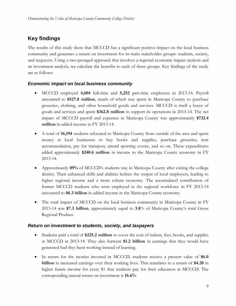
MCCCD employed 4,604 full-time and 5,252 part-time employees in 2013-14. Payroll
amounted to $527.8 million, much of which was spent in Maricopa County to purchase
groceries, clothing, and other household goods and services. MCCCD is itself a buyer of
goods and services and spent $362.8 million to support its operations in 2013-14. The net
impact of MCCCD payroll and expenses in Maricopa County was approximately $732.4
million in added income in FY 2013-14.
A total of 16,194 students relocated to Maricopa County from outside of the area and spent
money at local businesses to buy books and supplies, purchase groceries, rent
accommodation, pay for transport, attend sporting events, and so on. These expenditures
added approximately $240.6 million in income to the Maricopa County economy in FY
2013-14.
Approximately 89% of MCCCD’s students stay in Maricopa County after exiting the college
district. Their enhanced skills and abilities bolster the output of local employers, leading to
higher regional income and a more robust economy. The accumulated contribution of
former MCCCD students who were employed in the regional workforce in FY 2013-14
amounted to $6.3 billion in added income in the Maricopa County economy.
The total impact of MCCCD on the local business community in Maricopa County in FY
2013-14 was $7.3 billion, approximately equal to 3.8% of Maricopa County’s total Gross
Regional Product.
Return on investment to students, society, and taxpayers
Students paid a total of $225.2 million to cover the cost of tuition, fees, books, and supplies
at MCCCD in 2013-14. They also forwent $1.2 billion in earnings that they would have
generated had they been working instead of learning.
In return for the monies invested in MCCCD, students receive a present value of $6.0
billion in increased earnings over their working lives. This translates to a return of $4.20 in
higher future income for every $1 that students pay for their education at MCCCD. The
corresponding annual return on investment is 16.6%.

Demonstrating the Value of Maricopa County Community College District
10
Society as a whole in the state of Arizona will receive a present value of $25.7 billion in
added state income over the course of the students' working lives. Society will also benefit
from $337.9 million in present value social savings related to reduced crime, lower welfare
and unemployment, and increased health and well-being across the state.
For every dollar that society spent on MCCCD in FY 2013-14, society as a whole will receive
a cumulative value of $12.10 in benefits, for as long as MCCCD’s 2013-14 students remain
active in the state workforce.
State and local taxpayers in Arizona paid $499.0 million to support the operations of
MCCCD in 2013-14. The present value of the added tax revenue stemming from the
students' higher lifetime incomes and the increased output of businesses amounts to $1.9
billion in benefits to taxpayers. Savings to the public sector add another $111.9 million in
benefits due to a reduced demand for government-funded social services in Arizona.
Dividing the benefits to state and local taxpayers by the amount that they paid to support
MCCCD yields a 4.0 benefit-cost ratio, i.e., every $1 in costs returns $4.00 in benefits.
Taxpayers also see an average annual return of 10.3% on their investment in MCCCD.
Demonstrating the Value of Maricopa County Community College District
11
Chapter 1: Profile of MCCCD and the Regional
Economy
Estimating the benefits and costs of MCCCD requires three types of information: 1) employee and
finance data, 2) student demographic and achievement data, and 3) the economic profile of the
county and the state. For the purpose of this study, information on the district and its students was
obtained from MCCCD, and data on the regional and state economy were drawn from EMSI’s
proprietary data modeling tools.
1.1 Employee and finance data
1.1.1 Employee data
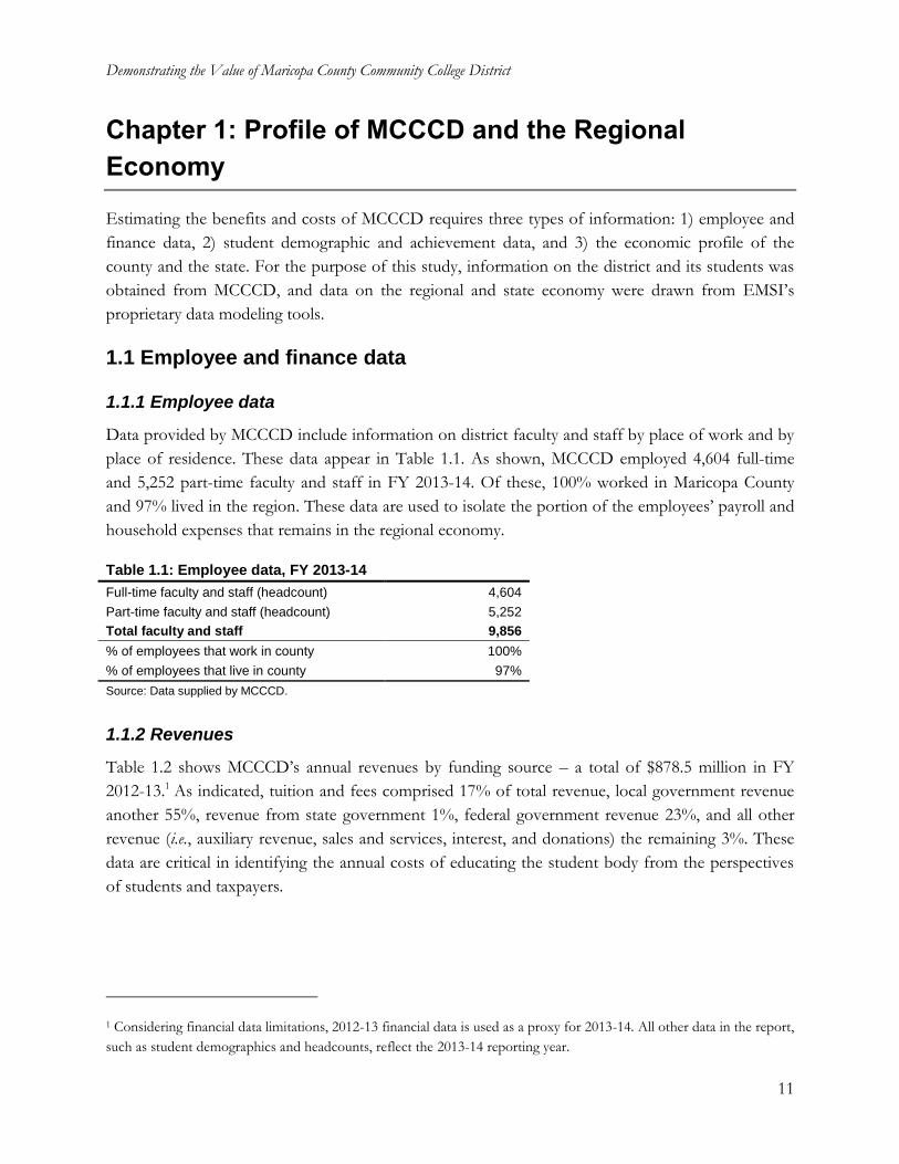
Data provided by MCCCD include information on district faculty and staff by place of work and by
place of residence. These data appear in Table 1.1. As shown, MCCCD employed 4,604 full-time
and 5,252 part-time faculty and staff in FY 2013-14. Of these, 100% worked in Maricopa County
and 97% lived in the region. These data are used to isolate the portion of the employees’ payroll and
household expenses that remains in the regional economy.
Table 1.1: Employee data, FY 2013-14
Full-time faculty and staff (headcount) 4,604
Part-time faculty and staff (headcount) 5,252
Total faculty and staff 9,856
% of employees that work in county 100%
% of employees that live in county 97%
Source: Data supplied by MCCCD.
1.1.2 Revenues
Table 1.2 shows MCCCD’s annual revenues by funding source – a total of $878.5 million in FY
2012-13.1 As indicated, tuition and fees comprised 17% of total revenue, local government revenue
another 55%, revenue from state government 1%, federal government revenue 23%, and all other
revenue (i.e., auxiliary revenue, sales and services, interest, and donations) the remaining 3%. These
data are critical in identifying the annual costs of educating the student body from the perspectives
of students and taxpayers.
1 Considering financial data limitations, 2012-13 financial data is used as a proxy for 2013-14. All other data in the report,
such as student demographics and headcounts, reflect the 2013-14 reporting year.
Demonstrating the Value of Maricopa County Community College District
12
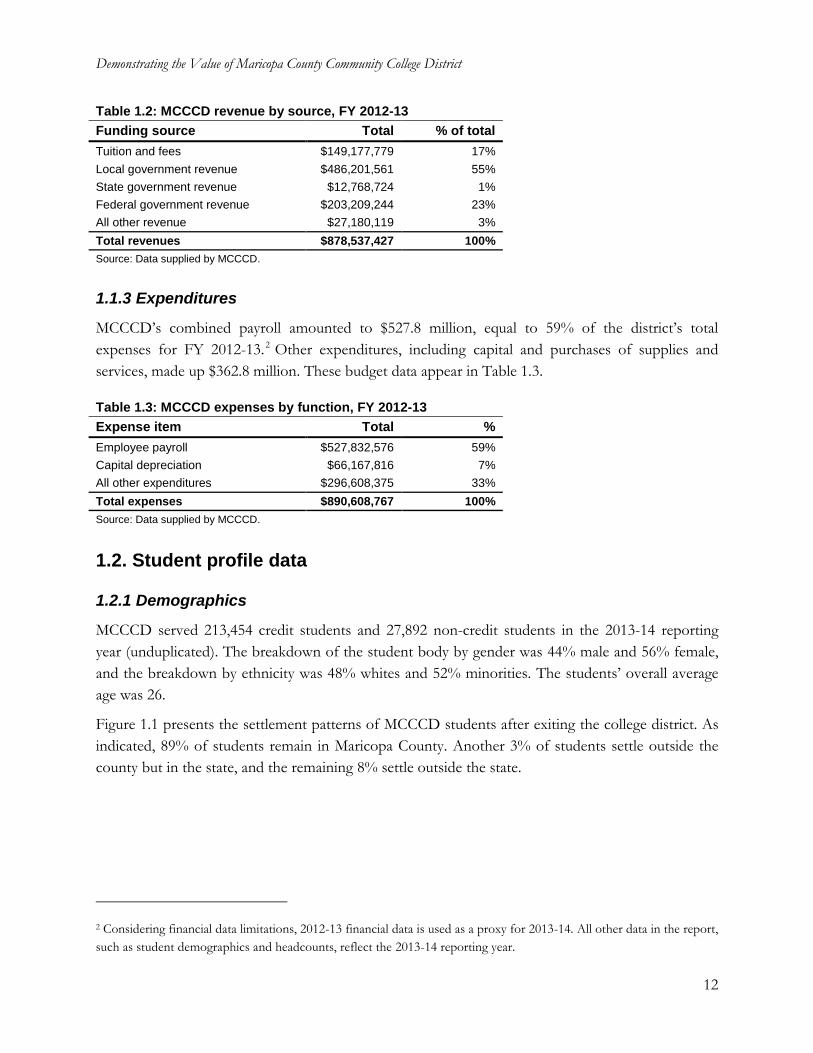
Table 1.2: MCCCD revenue by source, FY 2012-13
Funding source Total % of total
Tuition and fees $149,177,779 17%
Local government revenue $486,201,561 55%
State government revenue $12,768,724 1%
Federal government revenue $203,209,244 23%
All other revenue $27,180,119 3%
Total revenues $878,537,427 100%
Source: Data supplied by MCCCD.
1.1.3 Expenditures
MCCCD’s combined payroll amounted to $527.8 million, equal to 59% of the district’s total
expenses for FY 2012-13.2 Other expenditures, including capital and purchases of supplies and
services, made up $362.8 million. These budget data appear in Table 1.3.
Table 1.3: MCCCD expenses by function, FY 2012-13
Expense item Total %
Employee payroll $527,832,576 59%
Capital depreciation $66,167,816 7%
All other expenditures $296,608,375 33%
Total expenses $890,608,767 100%
Source: Data supplied by MCCCD.
1.2. Student profile data
1.2.1 Demographics
MCCCD served 213,454 credit students and 27,892 non-credit students in the 2013-14 reporting
year (unduplicated). The breakdown of the student body by gender was 44% male and 56% female,
and the breakdown by ethnicity was 48% whites and 52% minorities. The students’ overall average
age was 26.
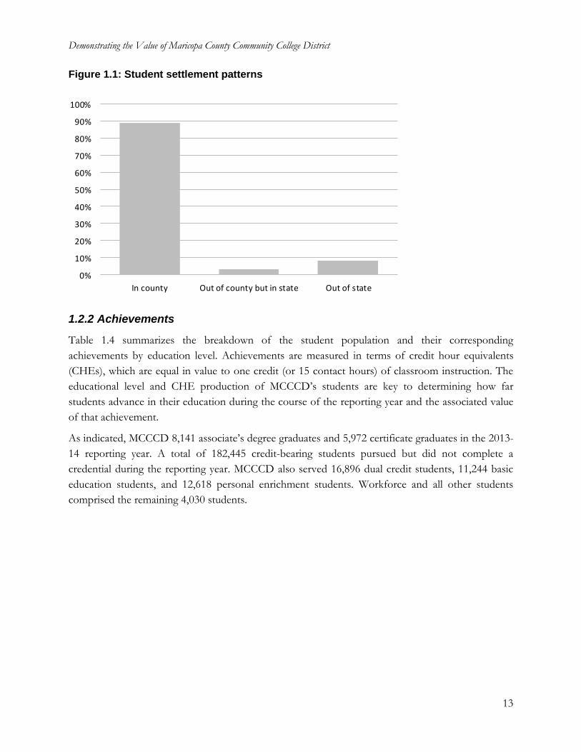
Figure 1.1 presents the settlement patterns of MCCCD students after exiting the college district. As
indicated, 89% of students remain in Maricopa County. Another 3% of students settle outside the
county but in the state, and the remaining 8% settle outside the state.
2 Considering financial data limitations, 2012-13 financial data is used as a proxy for 2013-14. All other data in the report,
such as student demographics and headcounts, reflect the 2013-14 reporting year.
Demonstrating the Value of Maricopa County Community College District
13
Figure 1.1: Student settlement patterns
0%
10%
20%
30%
40%
50%
60%
70%
80%
90%
100%
In county Out of county but in state Out of state
1.2.2 Achievements
Table 1.4 summarizes the breakdown of the student population and their corresponding
achievements by education level. Achievements are measured in terms of credit hour equivalents
(CHEs), which are equal in value to one credit (or 15 contact hours) of classroom instruction. The
educational level and CHE production of MCCCD’s students are key to determining how far
students advance in their education during the course of the reporting year and the associated value
of that achievement.
As indicated, MCCCD 8,141 associate’s degree graduates and 5,972 certificate graduates in the 2013-
14 reporting year. A total of 182,445 credit-bearing students pursued but did not complete a
credential during the reporting year. MCCCD also served 16,896 dual credit students, 11,244 basic
education students, and 12,618 personal enrichment students. Workforce and all other students
comprised the remaining 4,030 students.
Demonstrating the Value of Maricopa County Community College District
14
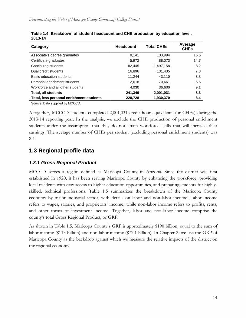
Table 1.4: Breakdown of student headcount and CHE production by education level, 2013-14
Category Headcount Total CHEs Average
CHEs
Associate’s degree graduates 8,141 133,994 16.5
Certificate graduates 5,972 88,073 14.7
Continuing students 182,445 1,497,158 8.2
Dual credit students 16,896 131,435 7.8
Basic education students 11,244 43,110 3.8
Personal enrichment students 12,618 70,661 5.6
Workforce and all other students 4,030 36,600 9.1
Total, all students 241,346 2,001,031 8.3
Total, less personal enrichment students 228,728 1,930,370 8.4
Source: Data supplied by MCCCD.
Altogether, MCCCD students completed 2,001,031 credit hour equivalents (or CHEs) during the
2013-14 reporting year. In the analysis, we exclude the CHE production of personal enrichment
students under the assumption that they do not attain workforce skills that will increase their
earnings. The average number of CHEs per student (excluding personal enrichment students) was
8.4.
1.3 Regional profile data
1.3.1 Gross Regional Product
MCCCD serves a region defined as Maricopa County in Arizona. Since the district was first
established in 1920, it has been serving Maricopa County by enhancing the workforce, providing
local residents with easy access to higher education opportunities, and preparing students for highly-
skilled, technical professions. Table 1.5 summarizes the breakdown of the Maricopa County
economy by major industrial sector, with details on labor and non-labor income. Labor income
refers to wages, salaries, and proprietors’ income; while non-labor income refers to profits, rents,
and other forms of investment income. Together, labor and non-labor income comprise the
county’s total Gross Regional Product, or GRP.
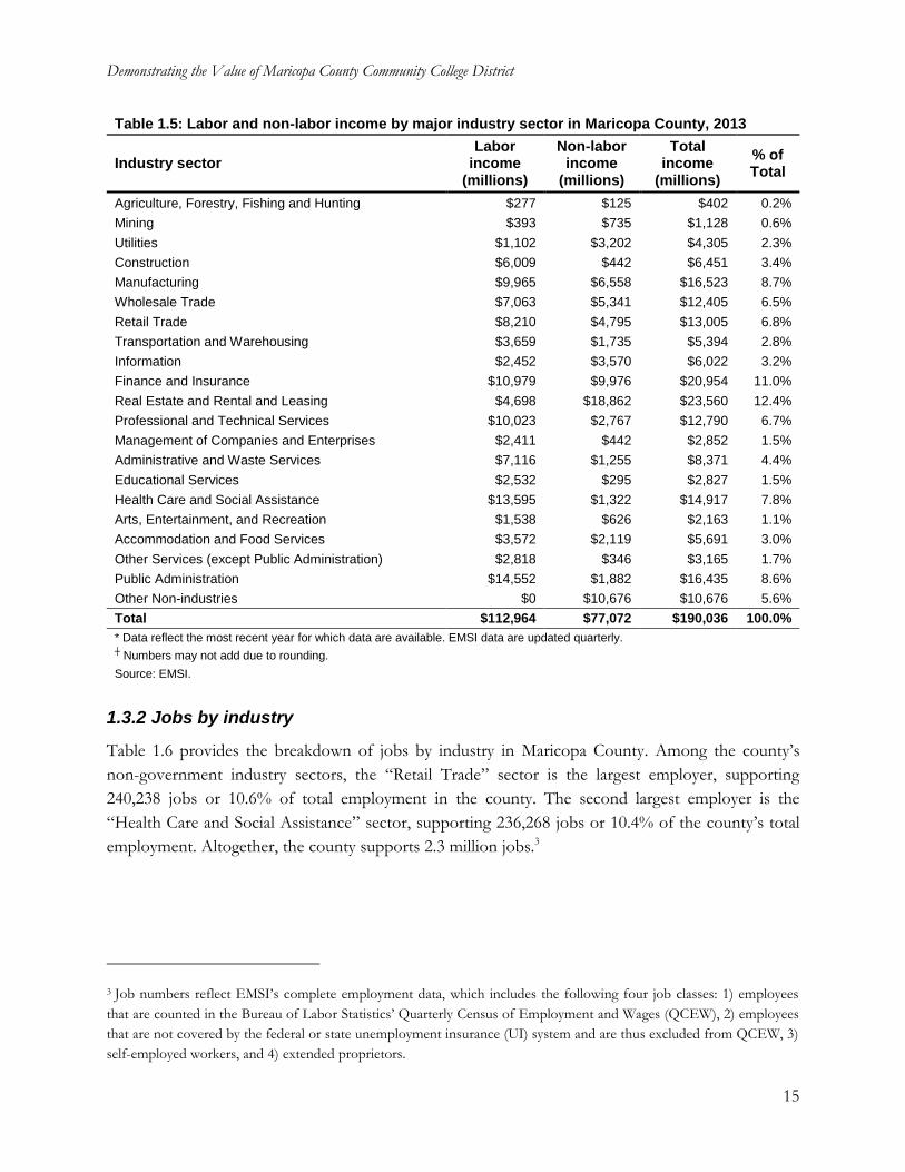
As shown in Table 1.5, Maricopa County’s GRP is approximately $190 billion, equal to the sum of
labor income ($113 billion) and non-labor income ($77.1 billion). In Chapter 2, we use the GRP of
Maricopa County as the backdrop against which we measure the relative impacts of the district on
the regional economy.
Demonstrating the Value of Maricopa County Community College District
15
Table 1.5: Labor and non-labor income by major industry sector in Maricopa County, 2013
Industry sector Labor
income (millions)
Non-labor income
(millions)
Total income
(millions)
% of Total
Agriculture, Forestry, Fishing and Hunting $277 $125 $402 0.2%
Mining $393 $735 $1,128 0.6%
Utilities $1,102 $3,202 $4,305 2.3%
Construction $6,009 $442 $6,451 3.4%
Manufacturing $9,965 $6,558 $16,523 8.7%
Wholesale Trade $7,063 $5,341 $12,405 6.5%
Retail Trade $8,210 $4,795 $13,005 6.8%
Transportation and Warehousing $3,659 $1,735 $5,394 2.8%
Information $2,452 $3,570 $6,022 3.2%
Finance and Insurance $10,979 $9,976 $20,954 11.0%
Real Estate and Rental and Leasing $4,698 $18,862 $23,560 12.4%
Professional and Technical Services $10,023 $2,767 $12,790 6.7%
Management of Companies and Enterprises $2,411 $442 $2,852 1.5%
Administrative and Waste Services $7,116 $1,255 $8,371 4.4%
Educational Services $2,532 $295 $2,827 1.5%
Health Care and Social Assistance $13,595 $1,322 $14,917 7.8%
Arts, Entertainment, and Recreation $1,538 $626 $2,163 1.1%
Accommodation and Food Services $3,572 $2,119 $5,691 3.0%
Other Services (except Public Administration) $2,818 $346 $3,165 1.7%
Public Administration $14,552 $1,882 $16,435 8.6%
Other Non-industries $0 $10,676 $10,676 5.6%
Total $112,964 $77,072 $190,036 100.0%
* Data reflect the most recent year for which data are available. EMSI data are updated quarterly. ┼ Numbers may not add due to rounding.
Source: EMSI.
1.3.2 Jobs by industry
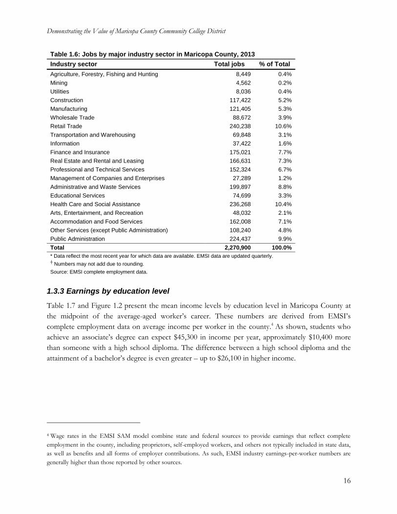
Table 1.6 provides the breakdown of jobs by industry in Maricopa County. Among the county’s
non-government industry sectors, the “Retail Trade” sector is the largest employer, supporting
240,238 jobs or 10.6% of total employment in the county. The second largest employer is the
“Health Care and Social Assistance” sector, supporting 236,268 jobs or 10.4% of the county’s total
employment. Altogether, the county supports 2.3 million jobs.3
3 Job numbers reflect EMSI’s complete employment data, which includes the following four job classes: 1) employees
that are counted in the Bureau of Labor Statistics’ Quarterly Census of Employment and Wages (QCEW), 2) employees
that are not covered by the federal or state unemployment insurance (UI) system and are thus excluded from QCEW, 3)
self-employed workers, and 4) extended proprietors.
Demonstrating the Value of Maricopa County Community College District
16
Table 1.6: Jobs by major industry sector in Maricopa County, 2013
Industry sector Total jobs % of Total
Agriculture, Forestry, Fishing and Hunting 8,449 0.4%
Mining 4,562 0.2%
Utilities 8,036 0.4%
Construction 117,422 5.2%
Manufacturing 121,405 5.3%
Wholesale Trade 88,672 3.9%
Retail Trade 240,238 10.6%
Transportation and Warehousing 69,848 3.1%
Information 37,422 1.6%
Finance and Insurance 175,021 7.7%
Real Estate and Rental and Leasing 166,631 7.3%
Professional and Technical Services 152,324 6.7%
Management of Companies and Enterprises 27,289 1.2%
Administrative and Waste Services 199,897 8.8%
Educational Services 74,699 3.3%
Health Care and Social Assistance 236,268 10.4%
Arts, Entertainment, and Recreation 48,032 2.1%
Accommodation and Food Services 162,008 7.1%
Other Services (except Public Administration) 108,240 4.8%
Public Administration 224,437 9.9%
Total 2,270,900 100.0%
* Data reflect the most recent year for which data are available. EMSI data are updated quarterly. ┼ Numbers may not add due to rounding.
Source: EMSI complete employment data.
1.3.3 Earnings by education level
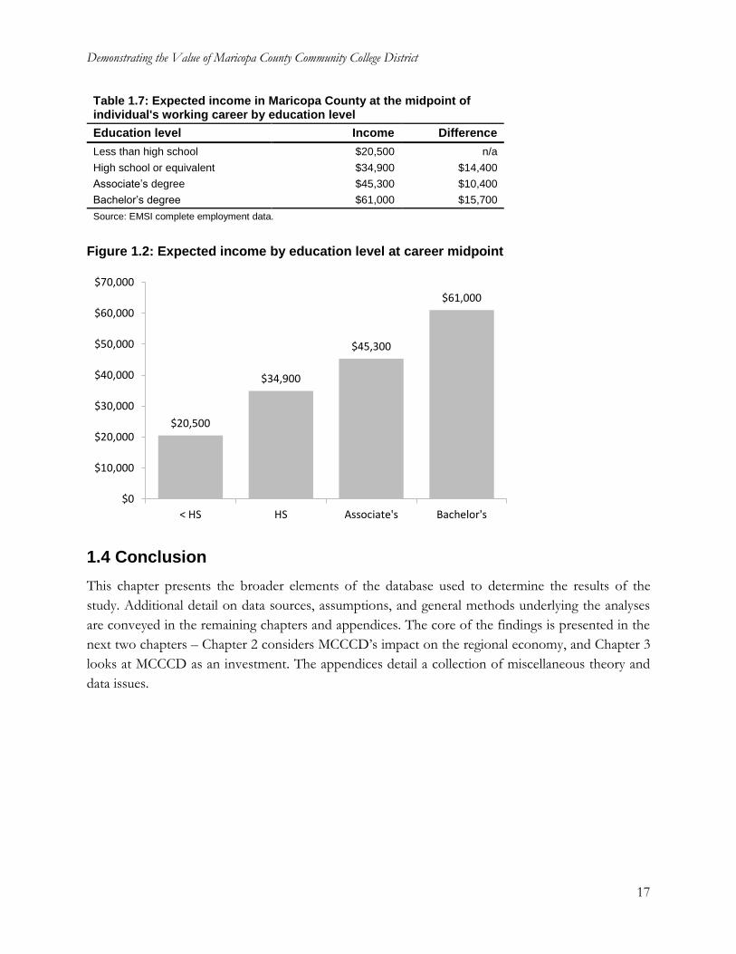
Table 1.7 and Figure 1.2 present the mean income levels by education level in Maricopa County at
the midpoint of the average-aged worker’s career. These numbers are derived from EMSI’s
complete employment data on average income per worker in the county.4 As shown, students who
achieve an associate’s degree can expect $45,300 in income per year, approximately $10,400 more
than someone with a high school diploma. The difference between a high school diploma and the
attainment of a bachelor’s degree is even greater – up to $26,100 in higher income.
4 Wage rates in the EMSI SAM model combine state and federal sources to provide earnings that reflect complete
employment in the county, including proprietors, self-employed workers, and others not typically included in state data,
as well as benefits and all forms of employer contributions. As such, EMSI industry earnings-per-worker numbers are
generally higher than those reported by other sources.
Demonstrating the Value of Maricopa County Community College District
17
Table 1.7: Expected income in Maricopa County at the midpoint of individual's working career by education level
Education level Income Difference
Less than high school $20,500 n/a
High school or equivalent $34,900 $14,400
Associate’s degree $45,300 $10,400
Bachelor’s degree $61,000 $15,700
Source: EMSI complete employment data.
Figure 1.2: Expected income by education level at career midpoint
1.4 Conclusion
This chapter presents the broader elements of the database used to determine the results of the
study. Additional detail on data sources, assumptions, and general methods underlying the analyses
are conveyed in the remaining chapters and appendices. The core of the findings is presented in the
next two chapters – Chapter 2 considers MCCCD’s impact on the regional economy, and Chapter 3
looks at MCCCD as an investment. The appendices detail a collection of miscellaneous theory and
data issues.
$20,500
$34,900
$45,300
$61,000
$0
$10,000
$20,000
$30,000
$40,000
$50,000
$60,000
$70,000
< HS HS Associate's Bachelor's
Demonstrating the Value of Maricopa County Community College District
18
Chapter 2: Economic Impact Analysis
MCCCD impacts Maricopa County in a variety of ways. The district is an employer and a buyer of
goods and services. It attracts monies to the county that would not have otherwise entered the local
economy through its own revenue stream and through the expenditures of non-local students.
Further, as a primary source of education to area residents, MCCCD supplies trained workers to
local industry and contributes to associated increases in regional output.
In this chapter we track MCCCD’s regional economic impact under three headings: 1) the district
operations impact, stemming from MCCCD’s payroll and purchases; 2) the student spending
impact, due to the spending of non-local students for room and board and other personal expenses,
and 3) the student productivity impact, comprising the added income created in the county as
former MCCCD students expand the economy’s stock of human capital.
2.1 District operations impact
Nearly all MCCCD employees live in Maricopa County (see Table 1.1). Faculty and staff payroll
counts as part of the county’s overall income, and their spending for groceries, apparel, and other
household expenditures helps support local businesses. MCCCD is itself a purchaser of supplies and
services, and many of MCCCD’s vendors are located in Maricopa County. These expenditures create
a ripple effect that generates still more jobs and income throughout the economy.
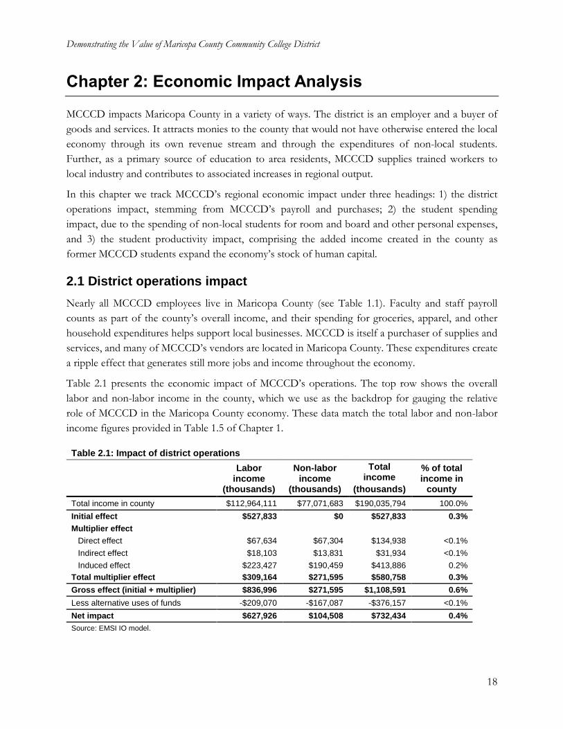
Table 2.1 presents the economic impact of MCCCD’s operations. The top row shows the overall
labor and non-labor income in the county, which we use as the backdrop for gauging the relative
role of MCCCD in the Maricopa County economy. These data match the total labor and non-labor
income figures provided in Table 1.5 of Chapter 1.
Table 2.1: Impact of district operations
Labor income
(thousands)
Non-labor income
(thousands)
Total income
(thousands)
% of total income in
county
Total income in county $112,964,111 $77,071,683 $190,035,794 100.0%
Initial effect $527,833 $0 $527,833 0.3%
Multiplier effect
Direct effect $67,634 $67,304 $134,938 <0.1%
Indirect effect $18,103 $13,831 $31,934 <0.1%
Induced effect $223,427 $190,459 $413,886 0.2%
Total multiplier effect $309,164 $271,595 $580,758 0.3%
Gross effect (initial + multiplier) $836,996 $271,595 $1,108,591 0.6%
Less alternative uses of funds -$209,070 -$167,087 -$376,157 <0.1%
Net impact $627,926 $104,508 $732,434 0.4%
Source: EMSI IO model.
Demonstrating the Value of Maricopa County Community College District
19
As for the impacts themselves, we follow best practice and draw the distinction between initial
effects and multiplier effects. The initial effect of MCCCD operations is simple – it amounts to the
$527.8 million in district payroll (including employee benefits). Total district payroll appeared in the
list of district expenditures reported in Table 1.3. Note that, as a public entity, MCCCD does not
generate property income in the traditional sense, so non-labor income is not associated with district
operations under the initial effect.
Multiplier effects refer to the additional income created in the economy as MCCCD and its
employees spend money in the county. They are categorized according to the following three effects:
the direct effect, the indirect effect, and the induced effect. Direct effects refer to the income created
by the industries initially affected by the spending of MCCCD and its employees. Indirect effects
occur as the supply chain of the initial industries creates even more income in the county. Finally,
induced effects refer to the income created by the increased spending of the household sector as a
result of the direct and indirect effects.
Calculating multiplier effects requires a specialized Social Accounting Matrix (SAM) model that
captures the interconnection of industries, government, and households in the county. The EMSI
SAM model contains approximately 1,100 industry sectors at the highest level of detail available in
the North American Industry Classification System (NAICS), and it supplies the industry-specific
multipliers required to determine the impacts associated with economic activity within the county.
For more information on the EMSI SAM model and its data sources, see Appendix 3.
Table 1.3 in Chapter 1 breaks MCCCD’s expenditures into the following three categories: payroll,
capital depreciation, and all other expenditures (including purchases for supplies and services). The
first step in estimating the multiplier effect of these expenditures is to map them individually to the
approximately 1,100 industry sectors of the EMSI SAM model. Assuming that the spending patterns
of district personnel approximately match those of the average consumer, we map district payroll to
spending on industry outputs using national household expenditure coefficients supplied by EMSI’s
national SAM. For the other two expenditure categories (i.e., capital depreciation and all other
expenditures), we again assume that the district’s spending patterns approximately match national
averages and apply the national spending coefficients for NAICS 611210 (Junior Colleges).5 Capital
depreciation is mapped to the construction sectors of NAICS 611210 and the district’s remaining
expenditures to the non-construction sectors of NAICS 611210.
We now have three vectors detailing the spending of MCCCD: one for district payroll, another for
capital items, and a third for MCCCD’s purchases of supplies and services. Before entering these
items into the SAM model, we factor out the portion of them that occurs locally. Each of the
approximately 1,100 sectors in the SAM model is represented by a regional purchase coefficient
(RPC), a measure of the overall demand for the commodities produced by each sector that is
satisfied by local suppliers. For example, if 40% of the demand for NAICS 541211 (Offices of
5 NAICS 611210 comprises junior colleges, community colleges, and junior college academies and schools.
Demonstrating the Value of Maricopa County Community College District
20
Certified Public Accountants) is satisfied by local suppliers, the RPC for that sector is 40%. The
remaining 60% of the demand for NAICS 541211 is provided by suppliers located outside the
county. The three district spending vectors are thus multiplied sector-by-sector by the corresponding
RPC for each sector to arrive at the strictly local spending associated with the district.
Local spending is entered into the SAM model’s multiplier matrix, which in turn provides an
estimate of the associated multiplier effects on regional sales. We convert the sales figures to income
using income-to-sales ratios, also provided by the SAM model. Final results appear in the section
labeled “Multiplier effect” in Table 2.1. Altogether, MCCCD’s spending creates $309.2 million in
labor income and another $271.6 million in non-labor income through multiplier effects – a total of
$580.8 million. This together with the $527.8 million in initial effects generates a gross total of $1.1
billion in impacts associated with the spending of MCCCD and its employees in the county.
Here we make a significant qualification. MCCCD received an estimated 72.0% of its funding from
sources in Maricopa County. These monies came from students living in the county, from private
sources located within the county, and from state and local taxes. 6 Had other industries received
these monies rather than MCCCD, income effects would have still been created in the economy.
This scenario is commonly known as a counterfactual outcome, i.e., what has not happened but what
would have happened if a given event – in this case, the expenditure of local funds on MCCCD –
had not occurred. In economic analysis, impacts that occur under counterfactual conditions are used
to offset the impacts that actually occur in order to derive the true impact of the event under
analysis.
For MCCCD, we calculate counterfactual outcomes by modeling the local monies spent on the
district as regular spending on consumer goods and savings. Our assumption is that, had students
not spent money on the district, they would have used that money instead to buy consumer goods.
Similarly, had the monies that taxpayers spent on MCCCD been returned to them in the form of a
tax decrease, we assume that they too would have spent that money on consumer goods. Our
approach, therefore, is to establish the total amount spent by local students and taxpayers on
MCCCD, map this to the detailed sectors of the SAM model using national household expenditure
coefficients, and scale the spending vector to reflect the change in local spending only. Finally, we
run the local spending through the SAM model’s regional multiplier matrix to derive initial and
multiplier effects, and then we convert the sales figures to income. The income effects of this new
consumer spending are shown as negative values in the row labeled “Less alternative uses of fund”
in Table 2.1.
The net total income impact of MCCCD spending can now be computed. As shown in the last row
of Table 2.1, the net impact is approximately $627.9 million in labor income and $104.5 million in
6 Local taxpayers pay state taxes, and it is thereby fair to assume that a portion of the state funds received by MCCCD
comes from local sources. The portion of state revenue paid by local taxpayers is estimated by applying the ratio of
regional earnings to total earnings in the state.
Demonstrating the Value of Maricopa County Community College District
21
non-labor income. The overall total is $732.4 million, representing the added income created in the
regional economy as a result of MCCCD operations.
2.2 Student spending impact
An estimated 16,194 of MCCCD’s students relocated to Maricopa County to attend the college
district in FY 2013-14. These students spent money at local businesses to purchase groceries, rent
accommodation, pay for transportation, and so on. The expenditures of MCCCD’s non-local
students supported local jobs and created new income in the regional economy.7
The average living expenses of students who relocated to Maricopa County appears in the first
section of Table 2.2, equal to $18,295 per student. Note that this figure excludes expenses for books
and supplies, since many of these monies are already reflected in the operations impact discussed in
the previous section. Multiplying the $18,295 in annual costs by the number of students who
relocated to the county (16,194 students) generates gross sales of $296.3 million.
Table 2.2: Average student cost of attendance and total sales generated by MCCCD’s non-local students in Maricopa County, 2013-14
Room and board $11,978
Personal expenses $6,317
Total expenses per student (A) $18,295
Number of MCCCD students who relocated to county (B) 16,194
Gross sales generated by students who relocated (A * B) $296,275,022
Source: Data on the cost of attendance and the number of students who relocated supplied by MCCCD.
Estimating the impacts generated by the $296.3 million in student spending follows a procedure
similar to that of the operations impact described above. We begin by mapping the $296.3 million in
sales to the industry sectors in the IO model, apply RPCs to reflect local spending only, and run the
net sales figures through the SAM model to derive multiplier effects. Finally, we convert the results
to income through the application of income-to-sales ratios.
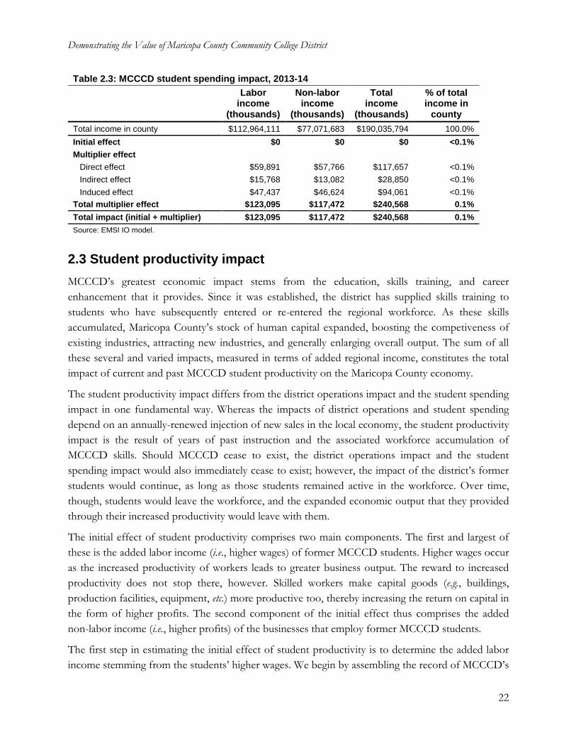
Table 2.3 presents the results Unlike the previous subsections, the initial effect is purely sales-
oriented and there is no change in labor or non-labor income. The impact of out-of-region student
spending thus falls entirely under the multiplier effect. The total impact of out-of-region student
spending is $240.6 million in added regional income. This value represents the direct added income
created at the businesses patronized by the students, the indirect added income created by the supply
chain of those businesses, and the increased spending of the household sector throughout the
regional economy as a result of the direct and indirect effects.
7 Online students and students who commuted to Maricopa County are not considered in this calculation because their
living expenses predominantly occurred in the region where they resided.
Demonstrating the Value of Maricopa County Community College District
22
Table 2.3: MCCCD student spending impact, 2013-14
Labor income
(thousands)
Non-labor income
(thousands)
Total income
(thousands)
% of total income in
county
Total income in county $112,964,111 $77,071,683 $190,035,794 100.0%
Initial effect $0 $0 $0 <0.1%
Multiplier effect
Direct effect $59,891 $57,766 $117,657 <0.1%
Indirect effect $15,768 $13,082 $28,850 <0.1%
Induced effect $47,437 $46,624 $94,061 <0.1%
Total multiplier effect $123,095 $117,472 $240,568 0.1%
Total impact (initial + multiplier) $123,095 $117,472 $240,568 0.1%
Source: EMSI IO model.
2.3 Student productivity impact
MCCCD’s greatest economic impact stems from the education, skills training, and career
enhancement that it provides. Since it was established, the district has supplied skills training to
students who have subsequently entered or re-entered the regional workforce. As these skills
accumulated, Maricopa County’s stock of human capital expanded, boosting the competiveness of
existing industries, attracting new industries, and generally enlarging overall output. The sum of all
these several and varied impacts, measured in terms of added regional income, constitutes the total
impact of current and past MCCCD student productivity on the Maricopa County economy.
The student productivity impact differs from the district operations impact and the student spending
impact in one fundamental way. Whereas the impacts of district operations and student spending
depend on an annually-renewed injection of new sales in the local economy, the student productivity
impact is the result of years of past instruction and the associated workforce accumulation of
MCCCD skills. Should MCCCD cease to exist, the district operations impact and the student
spending impact would also immediately cease to exist; however, the impact of the district’s former
students would continue, as long as those students remained active in the workforce. Over time,
though, students would leave the workforce, and the expanded economic output that they provided
through their increased productivity would leave with them.
The initial effect of student productivity comprises two main components. The first and largest of
these is the added labor income (i.e., higher wages) of former MCCCD students. Higher wages occur
as the increased productivity of workers leads to greater business output. The reward to increased
productivity does not stop there, however. Skilled workers make capital goods (e.g., buildings,
production facilities, equipment, etc.) more productive too, thereby increasing the return on capital in
the form of higher profits. The second component of the initial effect thus comprises the added
non-labor income (i.e., higher profits) of the businesses that employ former MCCCD students.
The first step in estimating the initial effect of student productivity is to determine the added labor
income stemming from the students’ higher wages. We begin by assembling the record of MCCCD’s
Demonstrating the Value of Maricopa County Community College District
23
historical student headcount (both credit and non-credit) over the past 30 years,8 from 1984-85 to
2013-14. From this vector of historical enrollments we remove the number of students who are not
currently active in the regional workforce, whether because they’re still enrolled in education, or
because they’re unemployed, employed but working in a different region, or out of the workforce
completely due to retirement or death. We estimate the historical employment patterns of students
in the county using the following sets of data or assumptions: 1) a set of settling-in factors to
determine how long it takes the average student to settle into a career;9 2) death, retirement, and
unemployment rates from the National Center for Health Statistics, the Social Security
Administration, and the Bureau of Labor Statistics; and 3) regional migration data from the U.S.
Census Bureau. The end result of these several computations is an estimate of the portion of
students who were still actively employed in the county as of FY 2013-14.
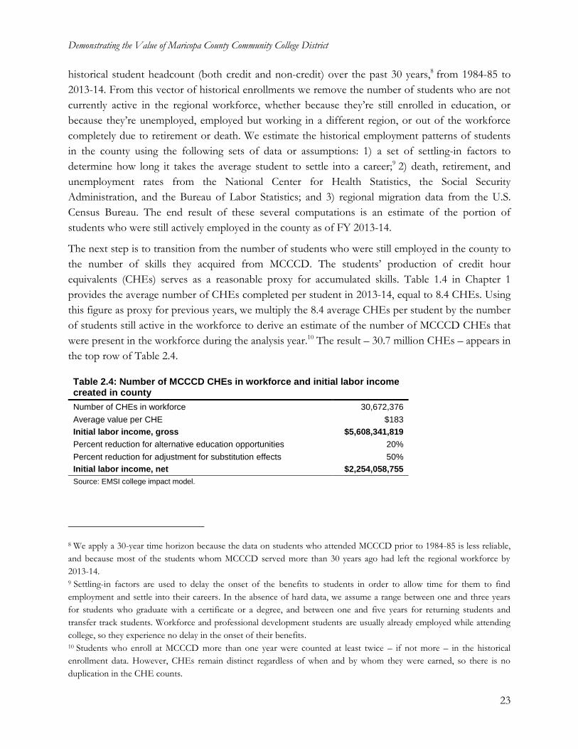
The next step is to transition from the number of students who were still employed in the county to
the number of skills they acquired from MCCCD. The students’ production of credit hour
equivalents (CHEs) serves as a reasonable proxy for accumulated skills. Table 1.4 in Chapter 1
provides the average number of CHEs completed per student in 2013-14, equal to 8.4 CHEs. Using
this figure as proxy for previous years, we multiply the 8.4 average CHEs per student by the number
of students still active in the workforce to derive an estimate of the number of MCCCD CHEs that
were present in the workforce during the analysis year.10 The result – 30.7 million CHEs – appears in
the top row of Table 2.4.
Table 2.4: Number of MCCCD CHEs in workforce and initial labor income created in county
Number of CHEs in workforce 30,672,376
Average value per CHE $183
Initial labor income, gross $5,608,341,819
Percent reduction for alternative education opportunities 20%
Percent reduction for adjustment for substitution effects 50%
Initial labor income, net $2,254,058,755
Source: EMSI college impact model.
8 We apply a 30-year time horizon because the data on students who attended MCCCD prior to 1984-85 is less reliable,
and because most of the students whom MCCCD served more than 30 years ago had left the regional workforce by
2013-14. 9 Settling-in factors are used to delay the onset of the benefits to students in order to allow time for them to find
employment and settle into their careers. In the absence of hard data, we assume a range between one and three years
for students who graduate with a certificate or a degree, and between one and five years for returning students and
transfer track students. Workforce and professional development students are usually already employed while attending
college, so they experience no delay in the onset of their benefits. 10 Students who enroll at MCCCD more than one year were counted at least twice – if not more – in the historical
enrollment data. However, CHEs remain distinct regardless of when and by whom they were earned, so there is no
duplication in the CHE counts.
Demonstrating the Value of Maricopa County Community College District
24
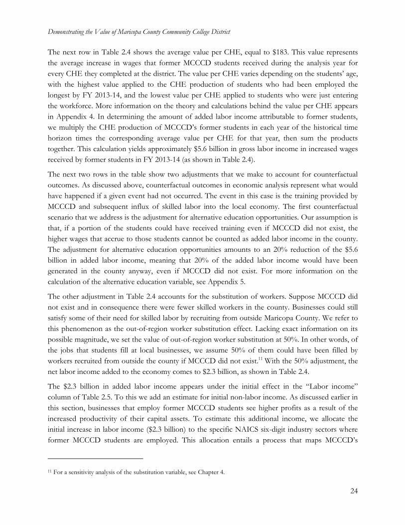
The next row in Table 2.4 shows the average value per CHE, equal to $183. This value represents
the average increase in wages that former MCCCD students received during the analysis year for
every CHE they completed at the district. The value per CHE varies depending on the students’ age,
with the highest value applied to the CHE production of students who had been employed the
longest by FY 2013-14, and the lowest value per CHE applied to students who were just entering
the workforce. More information on the theory and calculations behind the value per CHE appears
in Appendix 4. In determining the amount of added labor income attributable to former students,
we multiply the CHE production of MCCCD’s former students in each year of the historical time
horizon times the corresponding average value per CHE for that year, then sum the products
together. This calculation yields approximately $5.6 billion in gross labor income in increased wages
received by former students in FY 2013-14 (as shown in Table 2.4).
The next two rows in the table show two adjustments that we make to account for counterfactual
outcomes. As discussed above, counterfactual outcomes in economic analysis represent what would
have happened if a given event had not occurred. The event in this case is the training provided by
MCCCD and subsequent influx of skilled labor into the local economy. The first counterfactual
scenario that we address is the adjustment for alternative education opportunities. Our assumption is
that, if a portion of the students could have received training even if MCCCD did not exist, the
higher wages that accrue to those students cannot be counted as added labor income in the county.
The adjustment for alternative education opportunities amounts to an 20% reduction of the $5.6
billion in added labor income, meaning that 20% of the added labor income would have been
generated in the county anyway, even if MCCCD did not exist. For more information on the
calculation of the alternative education variable, see Appendix 5.
The other adjustment in Table 2.4 accounts for the substitution of workers. Suppose MCCCD did
not exist and in consequence there were fewer skilled workers in the county. Businesses could still
satisfy some of their need for skilled labor by recruiting from outside Maricopa County. We refer to
this phenomenon as the out-of-region worker substitution effect. Lacking exact information on its
possible magnitude, we set the value of out-of-region worker substitution at 50%. In other words, of
the jobs that students fill at local businesses, we assume 50% of them could have been filled by
workers recruited from outside the county if MCCCD did not exist.11 With the 50% adjustment, the
net labor income added to the economy comes to $2.3 billion, as shown in Table 2.4.
The $2.3 billion in added labor income appears under the initial effect in the “Labor income”
column of Table 2.5. To this we add an estimate for initial non-labor income. As discussed earlier in
this section, businesses that employ former MCCCD students see higher profits as a result of the
increased productivity of their capital assets. To estimate this additional income, we allocate the
initial increase in labor income ($2.3 billion) to the specific NAICS six-digit industry sectors where
former MCCCD students are employed. This allocation entails a process that maps MCCCD’s
11 For a sensitivity analysis of the substitution variable, see Chapter 4.
Demonstrating the Value of Maricopa County Community College District
25
completers12 to the detailed occupations for which those completers have been trained, and then
maps the detailed occupations to the six-digit industry sectors in the regional SAM model.
Completer data comes from the Integrated Postsecondary Education Data System (IPEDS), which
organizes MCCCD program completions according to the Classification of Instructional Programs
(CIP) developed by the National Center for Education Statistics (NCES). Using a crosswalk created
by NCES and the Bureau of Labor Statistics (BLS), we map the breakdown of MCCCD completers
by CIP code to the approximately 700 detailed occupations in the Standard Occupational
Classification (SOC) system used by the BLS. We then allocate the $2.3 billion in initial labor income
effects proportionately to the SOC framework based on the occupational distribution of the
completions. Finally, we apply a matrix of wages by industry and by occupation from the regional
SAM model to map the detailed occupational distribution of the $2.3 billion to the NAICS six-digit
industry sectors of the model.13
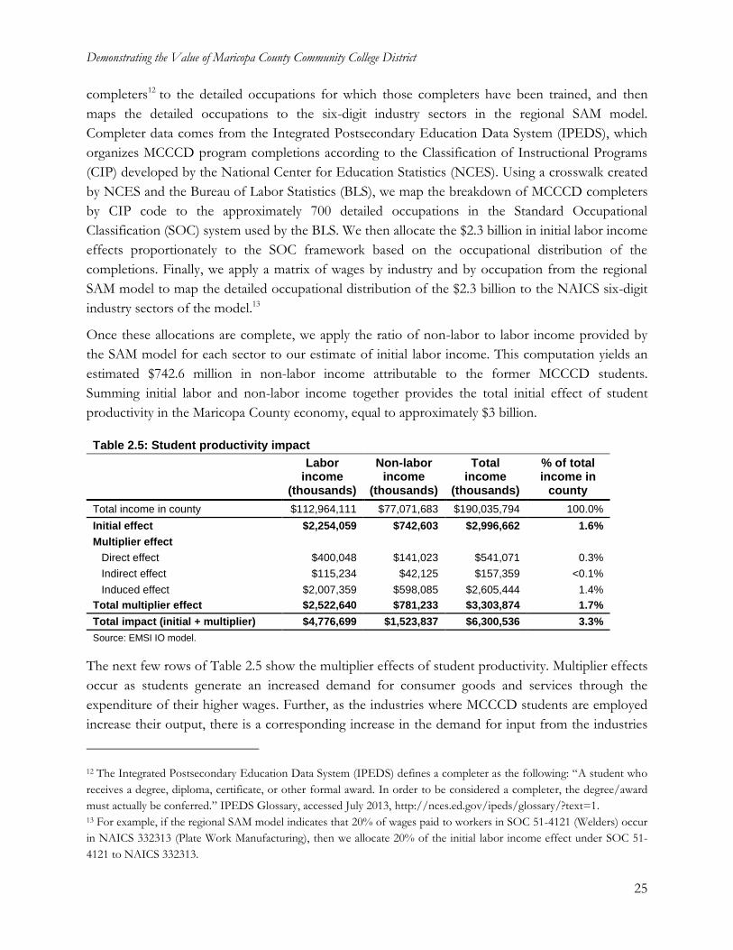
Once these allocations are complete, we apply the ratio of non-labor to labor income provided by
the SAM model for each sector to our estimate of initial labor income. This computation yields an
estimated $742.6 million in non-labor income attributable to the former MCCCD students.
Summing initial labor and non-labor income together provides the total initial effect of student
productivity in the Maricopa County economy, equal to approximately $3 billion.
Table 2.5: Student productivity impact
Labor income
(thousands)
Non-labor income
(thousands)
Total income
(thousands)
% of total income in
county
Total income in county $112,964,111 $77,071,683 $190,035,794 100.0%
Initial effect $2,254,059 $742,603 $2,996,662 1.6%
Multiplier effect
Direct effect $400,048 $141,023 $541,071 0.3%
Indirect effect $115,234 $42,125 $157,359 <0.1%
Induced effect $2,007,359 $598,085 $2,605,444 1.4%
Total multiplier effect $2,522,640 $781,233 $3,303,874 1.7%
Total impact (initial + multiplier) $4,776,699 $1,523,837 $6,300,536 3.3%
Source: EMSI IO model.
The next few rows of Table 2.5 show the multiplier effects of student productivity. Multiplier effects
occur as students generate an increased demand for consumer goods and services through the
expenditure of their higher wages. Further, as the industries where MCCCD students are employed
increase their output, there is a corresponding increase in the demand for input from the industries
12 The Integrated Postsecondary Education Data System (IPEDS) defines a completer as the following: “A student who
receives a degree, diploma, certificate, or other formal award. In order to be considered a completer, the degree/award
must actually be conferred.” IPEDS Glossary, accessed July 2013, http://nces.ed.gov/ipeds/glossary/?text=1. 13 For example, if the regional SAM model indicates that 20% of wages paid to workers in SOC 51-4121 (Welders) occur
in NAICS 332313 (Plate Work Manufacturing), then we allocate 20% of the initial labor income effect under SOC 51-
4121 to NAICS 332313.
Demonstrating the Value of Maricopa County Community College District
26
in the employers’ supply chain. Together, the incomes generated by the expansions in business input
purchases and household spending constitute the multiplier effect of the increased productivity of
former MCCCD students.
To estimate multiplier effects, we convert the industry-specific income figures generated through the
initial effect to regional sales using sales-to-income ratios from the SAM model. We then run the
values through the SAM’s multiplier matrix to determine the corresponding increases in industry
output that occur in the county. Finally, we convert all increases in regional sales back to income
using the income-to-sales ratios supplied by the SAM model. The final results are $2.5 billion in
labor income and $781.2 million in non-labor income, for an overall total of $3.3 billion in multiplier
effects. The grand total impact of student productivity thus comes to $6.3 billion, the sum of all
initial and multiplier labor and non-labor income effects. The total figures appear in the last row of
Table 2.5.
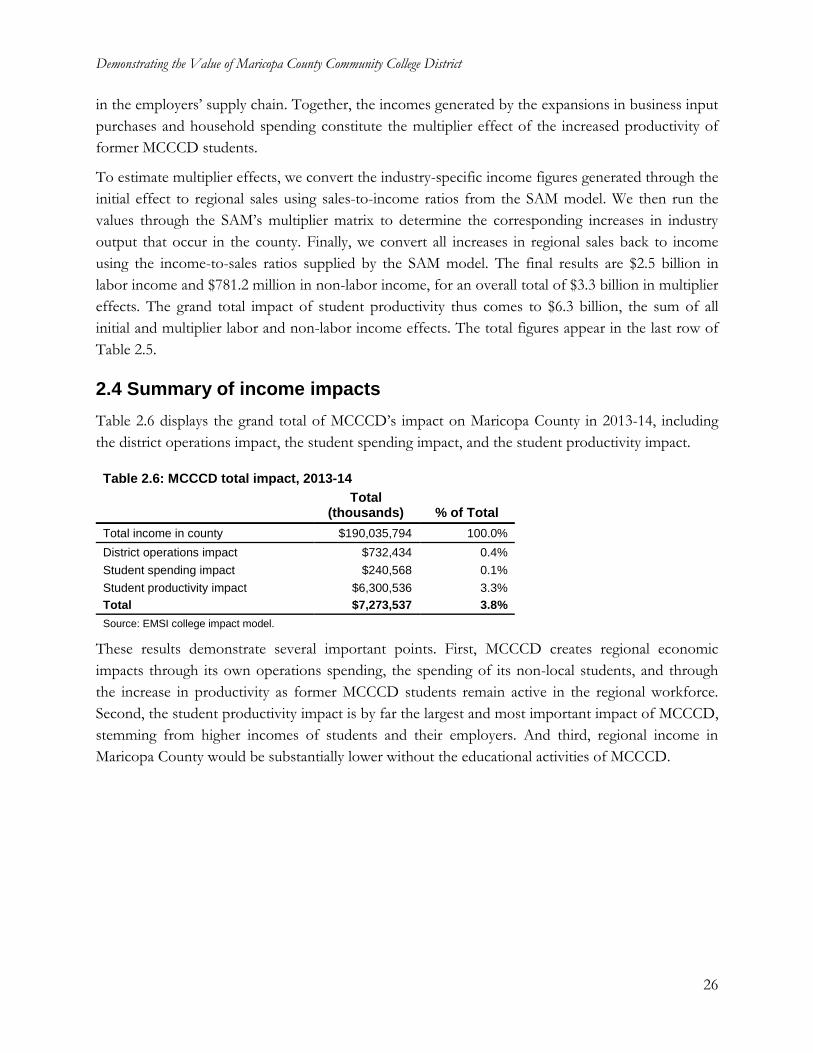
2.4 Summary of income impacts
Table 2.6 displays the grand total of MCCCD’s impact on Maricopa County in 2013-14, including
the district operations impact, the student spending impact, and the student productivity impact.
Table 2.6: MCCCD total impact, 2013-14
Total
(thousands) % of Total
Total income in county $190,035,794 100.0%
District operations impact $732,434 0.4%
Student spending impact $240,568 0.1%
Student productivity impact $6,300,536 3.3%
Total $7,273,537 3.8%
Source: EMSI college impact model.
These results demonstrate several important points. First, MCCCD creates regional economic
impacts through its own operations spending, the spending of its non-local students, and through
the increase in productivity as former MCCCD students remain active in the regional workforce.
Second, the student productivity impact is by far the largest and most important impact of MCCCD,
stemming from higher incomes of students and their employers. And third, regional income in
Maricopa County would be substantially lower without the educational activities of MCCCD.
Demonstrating the Value of Maricopa County Community College District
27
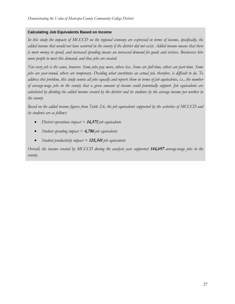
Calculating Job Equivalents Based on Income
In this study the impacts of MCCCD on the regional economy are expressed in terms of income, specifically, the
added income that would not have occurred in the county if the district did not exist. Added income means that there
is more money to spend, and increased spending means an increased demand for goods and services. Businesses hire
more people to meet this demand, and thus jobs are created.
Not every job is the same, however. Some jobs pay more, others less. Some are full-time, others are part-time. Some
jobs are year-round, others are temporary. Deciding what constitutes an actual job, therefore, is difficult to do. To
address this problem, this study counts all jobs equally and reports them in terms of job equivalents, i.e., the number
of average-wage jobs in the county that a given amount of income could potentially support. Job equivalents are
calculated by dividing the added income created by the district and its students by the average income per worker in
the county.
Based on the added income figures from Table 2.6, the job equivalents supported by the activities of MCCCD and
its students are as follows:
District operations impact = 14,571 job equivalents
Student spending impact = 4,786 job equivalents
Student productivity impact = 125,341 job equivalents
Overall, the income created by MCCCD during the analysis year supported 144,697 average-wage jobs in the
county.
Demonstrating the Value of Maricopa County Community College District
28
Chapter 3: Investment Analysis
Investment analysis is the process of evaluating total costs and measuring these against total benefits
to determine whether or not a proposed venture will be profitable. If benefits outweigh costs, then
the investment is worthwhile. If costs outweigh benefits, then the investment will lose money and is
thus considered infeasible. In this chapter, we consider MCCCD as an investment from the
perspectives of students, society, and taxpayers. The backdrop for the investment analysis for society
and taxpayers is the entire state of Arizona.
3.1 Student perspective
Analyzing the benefits and costs of education from the perspective of students is the most obvious
– they give up time and money to go to college in return for a lifetime of higher income. The cost
component of the analysis thus comprises the monies students pay (in the form of tuition and fees
and forgone time and money), and the benefit component focuses on the extent to which the
students’ incomes increase as a result of their education.
3.1.1 Calculating student costs
Student costs consist of two main items: direct outlays and opportunity costs. Direct outlays include
tuition and fees, equal to $149.2 million from Table 1.2. Direct outlays also include the cost of books
and supplies. On average, full-time students spent $1,264 each on books and supplies during the
reporting year.14 Multiplying this figure times the number of full-time equivalents (FTEs) produced
by MCCCD in 2013-1415 generates a total cost of $81.3 million for books and supplies.
Opportunity cost is the most difficult component of student costs to estimate. It measures the value
of time and earnings forgone by students who go to college rather than work. To calculate it, we
need to know the difference between the students’ full earning potential and what they actually earn
while attending college.
We derive the students’ full earning potential by weighting the average annual income levels in Table
1.7 according to the education level breakdown of the student population when they first enrolled.16
However, the income levels in Table 1.7 reflect what average workers earn at the midpoint of their
careers, not while attending college. Because of this, we adjust the income levels to the average age
14 Based on the data supplied by MCCCD. 15 A single FTE is equal to 30 CHEs, so there were 64,346 FTEs produced by MCCCD students in 2013-14, equal to
1,930,370 CHEs divided by 30 (excluding the CHE production of personal enrichment students). 16 Based on the number of students who reported their entry level of education to MCCCD.
Demonstrating the Value of Maricopa County Community College District
29
of the student population (26) to better reflect their wages at their current age.17 This calculation
yields an average full earning potential of $26,411 per student.
In determining what students earn while attending college, an important factor to consider is the
time that they actually spend at college, since this is the only time that they are required to give up a
portion of their earnings. We use the students’ CHE production as a proxy for time, under the
assumption that the more CHEs students earn, the less time they have to work, and, consequently,
the greater their forgone earnings. Overall, MCCCD students earned an average of 8.4 CHEs per
student (excluding personal enrichment students), which is approximately equal to 28% of a full
academic year. 18 We thus include no more than $7,430 (or 28%) of the students’ full earning
potential in the opportunity cost calculations.
Another factor to consider is the students’ employment status while attending the college district.
MCCCD estimates that 59% of its students are employed. For the 41% that are not working, we
assume that they are either seeking work or planning to seek work once they complete their
educational goals (with the exception of personal enrichment students, who are not included in this
calculation). By choosing to go to college, therefore, non-working students give up everything that
they can potentially earn during the academic year (i.e., the $7,430). The total value of their forgone
income thus comes to $696.8 million.
Working students are able to maintain all or part of their income while enrolled. However, many of
them hold jobs that pay less than statistical averages, usually because those are the only jobs they can
find that accommodate their course schedule. These jobs tend to be at entry level, such as restaurant
servers or cashiers. To account for this, we assume that working students hold jobs that pay 58% of
what they would have earned had they chosen to work full-time rather than go to college.19 The
remaining 42% comprises the percent of their full earning potential that they forgo. Obviously this
assumption varies by person – some students forego more and others less. Without knowing the
actual jobs that students hold while attending, however, the 42% in forgone earnings serves as a
reasonable average.
Working students also give up a portion of their leisure time in order to go to school, and
mainstream theory places a value on this.20 According to the Bureau of Labor Statistics American
17 We use the lifecycle earnings function identified by Jacob Mincer to scale the income levels to the students’ current
age. See Jacob Mincer, “Investment in Human Capital and Personal Income Distribution,” Journal of Political Economy, vol.
66 issue 4, August 1958: 281-302. Further discussion on the Mincer function and its role in calculating the students’
return on investment appears later in this chapter and in Appendix 4. 18 Equal to 8.4 CHEs divided by 30, the assumed number of CHEs in a full-time academic year. 19 The 58% assumption is based on the average hourly wage of the jobs most commonly held by working students
divided by the national average hourly wage. Occupational wage estimates are published by the Bureau of Labor
Statistics (see http://www.bls.gov/oes/current/oes_nat.htm). 20 See James M. Henderson and Richard E. Quandt, Microeconomic Theory: A Mathematical Approach (New York: McGraw-
Hill Book Company, 1971).
Demonstrating the Value of Maricopa County Community College District
30
Time Use Survey, students forgo up to 1.4 hours of leisure time per day.21 Assuming that an hour of
leisure is equal in value to an hour of work, we derive the total cost of leisure by multiplying the
number of leisure hours foregone during the academic year by the average hourly pay of the
students’ full earning potential. For working students, therefore, their total opportunity cost comes
to $597.5 million, equal to the sum of their foregone income ($425.1 million) and forgone leisure
time ($172.3 million).
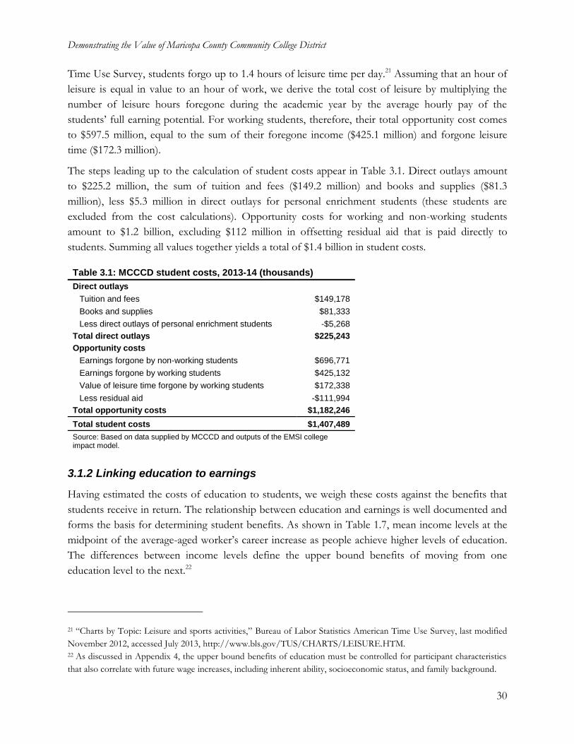
The steps leading up to the calculation of student costs appear in Table 3.1. Direct outlays amount
to $225.2 million, the sum of tuition and fees ($149.2 million) and books and supplies ($81.3
million), less $5.3 million in direct outlays for personal enrichment students (these students are
excluded from the cost calculations). Opportunity costs for working and non-working students
amount to $1.2 billion, excluding $112 million in offsetting residual aid that is paid directly to
students. Summing all values together yields a total of $1.4 billion in student costs.
Table 3.1: MCCCD student costs, 2013-14 (thousands)
Direct outlays
Tuition and fees $149,178
Books and supplies $81,333
Less direct outlays of personal enrichment students -$5,268
Total direct outlays $225,243
Opportunity costs
Earnings forgone by non-working students $696,771
Earnings forgone by working students $425,132
Value of leisure time forgone by working students $172,338
Less residual aid -$111,994
Total opportunity costs $1,182,246
Total student costs $1,407,489
Source: Based on data supplied by MCCCD and outputs of the EMSI college impact model.
3.1.2 Linking education to earnings
Having estimated the costs of education to students, we weigh these costs against the benefits that
students receive in return. The relationship between education and earnings is well documented and
forms the basis for determining student benefits. As shown in Table 1.7, mean income levels at the
midpoint of the average-aged worker’s career increase as people achieve higher levels of education.
The differences between income levels define the upper bound benefits of moving from one
education level to the next.22
21 “Charts by Topic: Leisure and sports activities,” Bureau of Labor Statistics American Time Use Survey, last modified
November 2012, accessed July 2013, http://www.bls.gov/TUS/CHARTS/LEISURE.HTM. 22 As discussed in Appendix 4, the upper bound benefits of education must be controlled for participant characteristics
that also correlate with future wage increases, including inherent ability, socioeconomic status, and family background.
Demonstrating the Value of Maricopa County Community College District
31
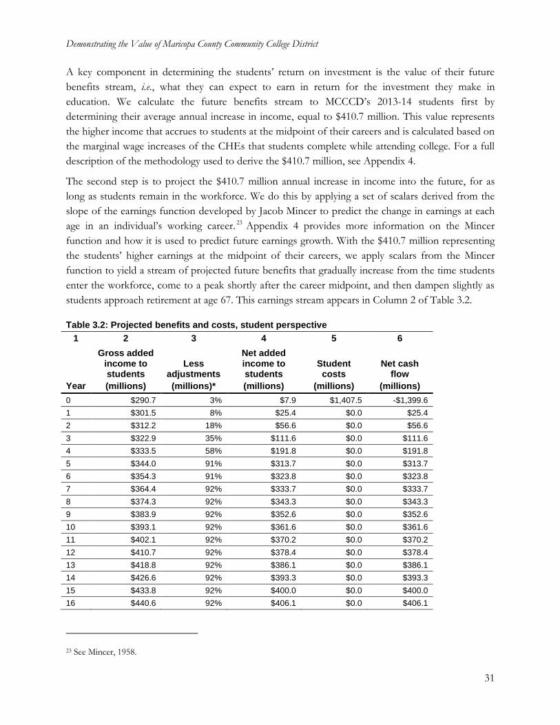
A key component in determining the students’ return on investment is the value of their future
benefits stream, i.e., what they can expect to earn in return for the investment they make in
education. We calculate the future benefits stream to MCCCD’s 2013-14 students first by
determining their average annual increase in income, equal to $410.7 million. This value represents
the higher income that accrues to students at the midpoint of their careers and is calculated based on
the marginal wage increases of the CHEs that students complete while attending college. For a full
description of the methodology used to derive the $410.7 million, see Appendix 4.
The second step is to project the $410.7 million annual increase in income into the future, for as
long as students remain in the workforce. We do this by applying a set of scalars derived from the
slope of the earnings function developed by Jacob Mincer to predict the change in earnings at each
age in an individual’s working career.23 Appendix 4 provides more information on the Mincer
function and how it is used to predict future earnings growth. With the $410.7 million representing
the students’ higher earnings at the midpoint of their careers, we apply scalars from the Mincer
function to yield a stream of projected future benefits that gradually increase from the time students
enter the workforce, come to a peak shortly after the career midpoint, and then dampen slightly as
students approach retirement at age 67. This earnings stream appears in Column 2 of Table 3.2.
Table 3.2: Projected benefits and costs, student perspective
1 2 3 4 5 6
Year
Gross added income to students
(millions)
Less adjustments
(millions)*
Net added income to students
(millions)
Student costs
(millions)
Net cash flow
(millions)
0 $290.7 3% $7.9 $1,407.5 -$1,399.6
1 $301.5 8% $25.4 $0.0 $25.4
2 $312.2 18% $56.6 $0.0 $56.6
3 $322.9 35% $111.6 $0.0 $111.6
4 $333.5 58% $191.8 $0.0 $191.8
5 $344.0 91% $313.7 $0.0 $313.7
6 $354.3 91% $323.8 $0.0 $323.8
7 $364.4 92% $333.7 $0.0 $333.7
8 $374.3 92% $343.3 $0.0 $343.3
9 $383.9 92% $352.6 $0.0 $352.6
10 $393.1 92% $361.6 $0.0 $361.6
11 $402.1 92% $370.2 $0.0 $370.2
12 $410.7 92% $378.4 $0.0 $378.4
13 $418.8 92% $386.1 $0.0 $386.1
14 $426.6 92% $393.3 $0.0 $393.3
15 $433.8 92% $400.0 $0.0 $400.0
16 $440.6 92% $406.1 $0.0 $406.1
23 See Mincer, 1958.
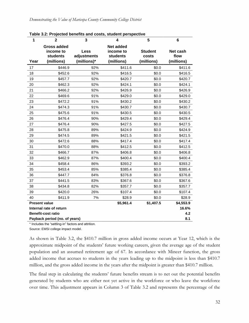
Demonstrating the Value of Maricopa County Community College District
32
Table 3.2: Projected benefits and costs, student perspective
1 2 3 4 5 6
Year
Gross added income to students
(millions)
Less adjustments
(millions)*
Net added income to students
(millions)
Student costs
(millions)
Net cash flow
(millions)
17 $446.9 92% $411.6 $0.0 $411.6
18 $452.6 92% $416.5 $0.0 $416.5
19 $457.7 92% $420.7 $0.0 $420.7
20 $462.3 92% $424.1 $0.0 $424.1
21 $466.2 92% $426.9 $0.0 $426.9
22 $469.6 91% $429.0 $0.0 $429.0
23 $472.2 91% $430.2 $0.0 $430.2
24 $474.3 91% $430.7 $0.0 $430.7
25 $475.6 91% $430.5 $0.0 $430.5
26 $476.4 90% $429.4 $0.0 $429.4
27 $476.4 90% $427.5 $0.0 $427.5
28 $475.8 89% $424.9 $0.0 $424.9
29 $474.5 89% $421.5 $0.0 $421.5
30 $472.6 88% $417.4 $0.0 $417.4
31 $470.0 88% $412.5 $0.0 $412.5
32 $466.7 87% $406.8 $0.0 $406.8
33 $462.9 87% $400.4 $0.0 $400.4
34 $458.4 86% $393.2 $0.0 $393.2
35 $453.4 85% $385.4 $0.0 $385.4
36 $447.7 84% $376.8 $0.0 $376.8
37 $441.5 83% $367.6 $0.0 $367.6
38 $434.8 82% $357.7 $0.0 $357.7
39 $420.0 26% $107.4 $0.0 $107.4
40 $411.9 7% $28.9 $0.0 $28.9
Present value $5,961.4 $1,407.5 $4,553.9
Internal rate of return
16.6%
Benefit-cost ratio
4.2
Payback period (no. of years) 8.1
* Includes the “settling-in” factors and attrition.
Source: EMSI college impact model.
As shown in Table 3.2, the $410.7 million in gross added income occurs at Year 12, which is the
approximate midpoint of the students’ future working careers, given the average age of the student
population and an assumed retirement age of 67. In accordance with Mincer function, the gross
added income that accrues to students in the years leading up to the midpoint is less than $410.7
million, and the gross added income in the years after the midpoint is greater than $410.7 million.
The final step in calculating the students’ future benefits stream is to net out the potential benefits
generated by students who are either not yet active in the workforce or who leave the workforce
over time. This adjustment appears in Column 3 of Table 3.2 and represents the percentage of the
Demonstrating the Value of Maricopa County Community College District
33
total 2013-14 student population that will be employed in the workforce in a given year. Note that
the percentages in the first five years of the time horizon are relatively lower than those in
subsequent years. This is because many students delay their entry into the workforce, either because
they are still enrolled at the district or because they are unable to find a job immediately upon
graduation. Accordingly, we apply a set of “settling-in” factors to account for the time needed by
students to find employment and settle into their careers. As discussed in Chapter 2, settling-in
factors delay the onset of the benefits by one to three years for students who graduate with a
certificate or a degree, and by one to five years for returning students and transfer track students. We
apply no settling-in factors to the benefits for workforce and professional development students
because the majority of them are employed while attending.
Beyond the first five years of the time horizon, students will leave the workforce over time for any
number of reasons, whether because of death, retirement, or unemployment. We estimate the rate of
attrition using the same data and assumptions applied in the calculation of the attrition rate in the
economic impact analysis of Chapter 2.24 The likelihood that students leave the workforce increases
as they age, so the attrition rate is more aggressive near the end of the time horizon than in the
beginning. Column 4 of Table 3.2 shows the net added income to students after accounting for both
the settling-in patterns and attrition.
3.1.3 Return on investment to students
Having estimated the students’ costs and their future benefits stream, the next step is to discount the
results to the present to reflect the time value of money. For the student perspective we assume a
discount rate of 4.5% (see the “Discount Rate” box).25 The present value of the benefits is then
compared to student costs to derive the investment analysis results, expressed in terms of a benefit-
cost ratio, rate of return, and payback period. The investment is feasible if returns match or exceed
the minimum threshold values, i.e., a benefit-cost ratio greater than 1, a rate of return that exceeds
the discount rate, and a reasonably short payback period.
Discount Rate
The discount rate is a rate of interest that converts future costs and benefits to present values. For example, $1,000
in higher earnings realized 30 years in the future is worth much less than $1,000 in the present. All future values
must therefore be expressed in present value terms in order to compare them with investments (i.e., costs) made
24 See the discussion of the student productivity effect in Chapter 2. The main sources for deriving the attrition rate are
the National Center for Health Statistics, the Social Security Administration, and the Bureau of Labor Statistics. Note
that we do not account for migration patterns in the student investment analysis because the higher earnings that
students receive as a result of their education will accrue to them regardless of where they find employment. 25 The student discount rate is derived from the baseline forecasts for the ten-year zero coupon bond discount rate
published by the Congressional Budget Office. See the Congressional Budget Office, Student Loan and Pell Grant
Programs - March 2012 Baseline, Congressional Budget Office Publications, last modified March 13, 2012, accessed July
2013, http://www.cbo.gov/sites/default/files/cbofiles/attachments/43054_StudentLoanPellGrantPrograms.pdf.
Demonstrating the Value of Maricopa County Community College District
34
today. The selection of an appropriate discount rate, however, can become an arbitrary and controversial
undertaking. As suggested in economic theory, the discount rate should reflect the investor’s opportunity cost of
capital, i.e., the rate of return one could reasonably expect to obtain from alternative investment schemes. In this
study we assume a 4.5% discount rate from the student perspective and a 1.1% discount rate from the taxpayer
perspective. The discount rate for taxpayers is lower than it is for students because governments are large and can
therefore spread their risks over a larger and more diverse investment portfolio than the private sector can.
In Table 3.2, the net added income of MCCCD students yields a cumulative discounted sum of
approximately $6 billion, the present value of all of the future income increments (see the bottom
section of Column 4). This may also be interpreted as the gross capital asset value of the students’
higher income stream. In effect, the aggregate 2013-14 student body is rewarded for their
investment in MCCCD with a capital asset valued at $6 billion.
The students’ cost of attending MCCCD is shown in Column 5 of Table 3.2, equal to a present
value of $1.4 billion. Note that costs only occur in the single analysis year and are thus already in
current year dollars. Comparing the cost with the present value of benefits yields a student benefit-
cost ratio of 4.2 (equal to $6 billion in benefits divided by $1.4 billion in costs).
Another way to compare the same benefits stream and associated cost is to compute the rate of
return. The rate of return indicates the interest rate that a bank would have to pay a depositor to
yield an equally attractive stream of future payments.26 Table 3.2 shows MCCCD students earning
average returns of 16.6% on their investment of time and money. This is a favorable return
compared, for example, to approximately 1% on a standard bank savings account, or 7% on stocks
and bonds (thirty-year average return).
Note that returns reported in this study are real returns, not nominal. When a bank promises to pay
a certain rate of interest on a savings account, it employs an implicitly nominal rate. Bonds operate
in a similar manner. If it turns out that the inflation rate is higher than the stated rate of return, then
money is lost in real terms. In contrast, a real rate of return is on top of inflation. For example, if
inflation is running at 3% and a nominal percentage of 5% is paid, then the real rate of return on the
investment is only 2%. In Table 3.2, the 16.6% student rate of return is a real rate. With an inflation
rate of 2.5% (the average rate reported over the past 20 years as per the U.S. Department of
Commerce, Consumer Price Index), the corresponding nominal rate of return is 19.1%, substantially
higher than what is reported in Table 3.2.
26 Rates of return are computed using the familiar “internal rate of return” calculation. Note that, with a bank deposit or
stock market investment, the depositor puts up a principal, receives in return a stream of periodic payments, and then
recovers the principal at the end. Someone who invests in education, on the other hand, receives a stream of periodic
payments that include the recovery of the principal as part of the periodic payments, but there is no principal recovery at
the end. These differences notwithstanding, comparable cash flows for both bank and education investors yield the same
internal rate of return.
Demonstrating the Value of Maricopa County Community College District
35
The payback period is defined as the length of time it takes to entirely recoup the initial
investment.27 Beyond that point, returns are what economists would call “pure costless rent.” As
indicated in Table 3.2, students at MCCCD see, on average, a payback period of 8.1 years on their
forgone earnings and out-of-pocket costs.
3.2 Social perspective
Society as a whole in Arizona benefits from the education that MCCCD provides through the
income that students create in the state and through the savings that they generate through their
improved lifestyles. To receive these benefits, however, members of society must pay money and
forgo services that they would have otherwise enjoyed if MCCCD did not exist. Society’s investment
in MCCCD stretches across a number of investor groups, from students to employers to taxpayers.
We weigh the benefits generated by MCCCD to society against the total societal costs of generating
those benefits. The total societal costs include all MCCCD expenditures, all student expenditures,
and all student opportunity costs, totaling $2148.9 million (= $890.6 million in MCCCD
expenditures + $76.1 million in student expenditures + $1.2 billion in student opportunity costs).
On the benefits side, any benefits that accrue to society as a whole – including students, employers,
taxpayers, and anyone else who stands to benefit from the activities of MCCCD – are counted as
benefits under the social perspective. We group these benefits under the following broad headings:
1) increased income in the state, and 2) social externalities stemming from improved health, reduced
crime, and reduced unemployment in the state (see the “Beekeeper Analogy” box for a discussion of
externalities). Both of these benefits components are described more fully in the following sections.
27 Payback analysis is generally used by the business community to rank alternative investments when safety of
investments is an issue. Its greatest drawback is that it takes no account of the time value of money. The payback period
is calculated by dividing the cost of the investment by the net return per period. In this study, the cost of the investment
includes tuition and fees plus the opportunity cost of time – it does not take into account student living expenses or
interest on loans.
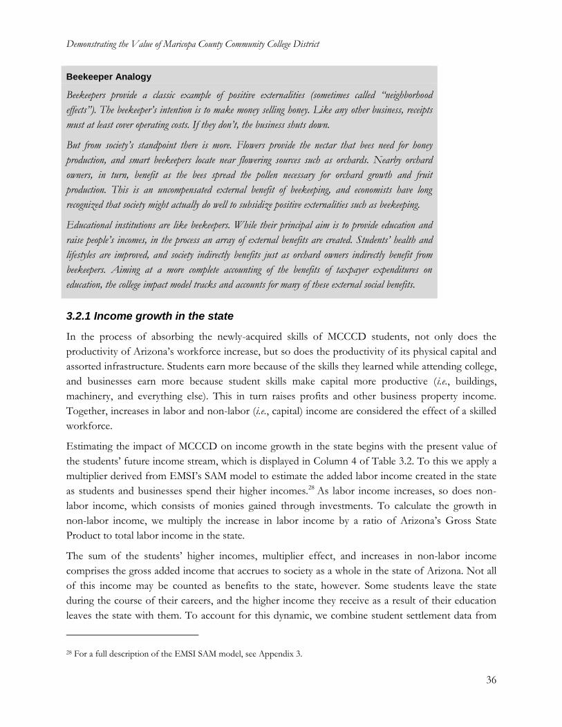
Demonstrating the Value of Maricopa County Community College District
36
Beekeeper Analogy
Beekeepers provide a classic example of positive externalities (sometimes called “neighborhood
effects”). The beekeeper’s intention is to make money selling honey. Like any other business, receipts
must at least cover operating costs. If they don’t, the business shuts down.
But from society’s standpoint there is more. Flowers provide the nectar that bees need for honey
production, and smart beekeepers locate near flowering sources such as orchards. Nearby orchard
owners, in turn, benefit as the bees spread the pollen necessary for orchard growth and fruit
production. This is an uncompensated external benefit of beekeeping, and economists have long
recognized that society might actually do well to subsidize positive externalities such as beekeeping.
Educational institutions are like beekeepers. While their principal aim is to provide education and
raise people’s incomes, in the process an array of external benefits are created. Students’ health and
lifestyles are improved, and society indirectly benefits just as orchard owners indirectly benefit from
beekeepers. Aiming at a more complete accounting of the benefits of taxpayer expenditures on
education, the college impact model tracks and accounts for many of these external social benefits.
3.2.1 Income growth in the state
In the process of absorbing the newly-acquired skills of MCCCD students, not only does the
productivity of Arizona’s workforce increase, but so does the productivity of its physical capital and
assorted infrastructure. Students earn more because of the skills they learned while attending college,
and businesses earn more because student skills make capital more productive (i.e., buildings,
machinery, and everything else). This in turn raises profits and other business property income.
Together, increases in labor and non-labor (i.e., capital) income are considered the effect of a skilled
workforce.
Estimating the impact of MCCCD on income growth in the state begins with the present value of
the students’ future income stream, which is displayed in Column 4 of Table 3.2. To this we apply a
multiplier derived from EMSI’s SAM model to estimate the added labor income created in the state
as students and businesses spend their higher incomes.28 As labor income increases, so does non-
labor income, which consists of monies gained through investments. To calculate the growth in
non-labor income, we multiply the increase in labor income by a ratio of Arizona’s Gross State
Product to total labor income in the state.
The sum of the students’ higher incomes, multiplier effect, and increases in non-labor income
comprises the gross added income that accrues to society as a whole in the state of Arizona. Not all
of this income may be counted as benefits to the state, however. Some students leave the state
during the course of their careers, and the higher income they receive as a result of their education
leaves the state with them. To account for this dynamic, we combine student settlement data from
28 For a full description of the EMSI SAM model, see Appendix 3.
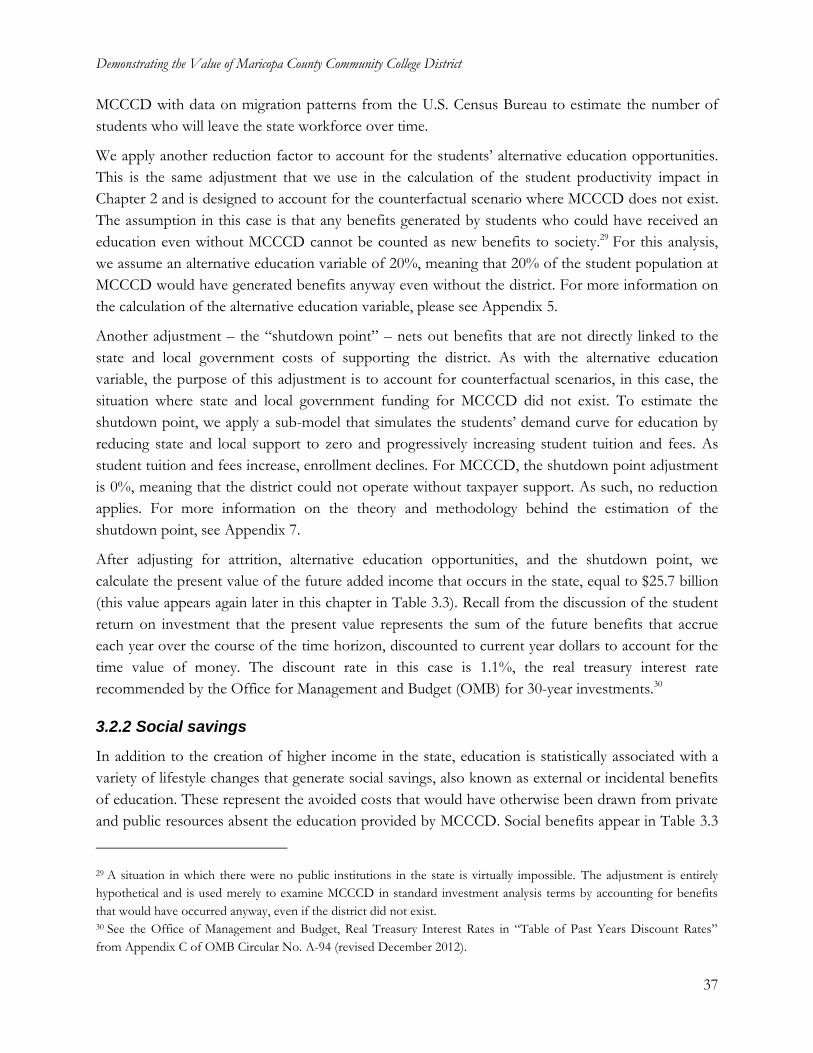
Demonstrating the Value of Maricopa County Community College District
37
MCCCD with data on migration patterns from the U.S. Census Bureau to estimate the number of
students who will leave the state workforce over time.
We apply another reduction factor to account for the students’ alternative education opportunities.
This is the same adjustment that we use in the calculation of the student productivity impact in
Chapter 2 and is designed to account for the counterfactual scenario where MCCCD does not exist.
The assumption in this case is that any benefits generated by students who could have received an
education even without MCCCD cannot be counted as new benefits to society.29 For this analysis,
we assume an alternative education variable of 20%, meaning that 20% of the student population at
MCCCD would have generated benefits anyway even without the district. For more information on
the calculation of the alternative education variable, please see Appendix 5.
Another adjustment – the “shutdown point” – nets out benefits that are not directly linked to the
state and local government costs of supporting the district. As with the alternative education
variable, the purpose of this adjustment is to account for counterfactual scenarios, in this case, the
situation where state and local government funding for MCCCD did not exist. To estimate the
shutdown point, we apply a sub-model that simulates the students’ demand curve for education by
reducing state and local support to zero and progressively increasing student tuition and fees. As
student tuition and fees increase, enrollment declines. For MCCCD, the shutdown point adjustment
is 0%, meaning that the district could not operate without taxpayer support. As such, no reduction
applies. For more information on the theory and methodology behind the estimation of the
shutdown point, see Appendix 7.
After adjusting for attrition, alternative education opportunities, and the shutdown point, we
calculate the present value of the future added income that occurs in the state, equal to $25.7 billion
(this value appears again later in this chapter in Table 3.3). Recall from the discussion of the student
return on investment that the present value represents the sum of the future benefits that accrue
each year over the course of the time horizon, discounted to current year dollars to account for the
time value of money. The discount rate in this case is 1.1%, the real treasury interest rate
recommended by the Office for Management and Budget (OMB) for 30-year investments.30
3.2.2 Social savings
In addition to the creation of higher income in the state, education is statistically associated with a
variety of lifestyle changes that generate social savings, also known as external or incidental benefits
of education. These represent the avoided costs that would have otherwise been drawn from private
and public resources absent the education provided by MCCCD. Social benefits appear in Table 3.3
29 A situation in which there were no public institutions in the state is virtually impossible. The adjustment is entirely
hypothetical and is used merely to examine MCCCD in standard investment analysis terms by accounting for benefits
that would have occurred anyway, even if the district did not exist. 30 See the Office of Management and Budget, Real Treasury Interest Rates in “Table of Past Years Discount Rates”
from Appendix C of OMB Circular No. A-94 (revised December 2012).
Demonstrating the Value of Maricopa County Community College District
38
and break down into three main categories: 1) health savings, 2) crime savings, and 3) welfare and
unemployment savings. Health savings include avoided medical costs, lost productivity, and other
effects associated with smoking, alcoholism, obesity, mental illness, and drug abuse. Crime savings
consist of avoided costs to the justice system (i.e., police protection, judicial and legal, and
corrections), avoided victim costs, and benefits stemming from the added productivity of individuals
who would have otherwise been incarcerated. Welfare and unemployment benefits comprise
avoided costs due to the reduced number of social assistance and unemployment insurance claims.
The model quantifies social savings by calculating the probability at each education level that
individuals will have poor health, commit crimes, or claim welfare and unemployment benefits.
Deriving the probabilities involves assembling data from a variety of studies and surveys analyzing
the correlation between education and health, crime, welfare, and unemployment at the national and
state level. We spread the probabilities across the education ladder and multiply the marginal
differences by the number of students who achieved CHEs at each step. The sum of these marginal
differences counts as the upper bound measure of the number of students who, due to the
education they received at MCCCD, will not have poor health, commit crimes, or claim welfare and
unemployment benefits. We dampen these results by the “ability bias” adjustment discussed earlier
in this chapter and in Appendix 4 to account for other factors besides education that influence
individual behavior. We then multiply the marginal effects of education times the associated costs of
health, crime, welfare, and unemployment.31 Finally, we apply the same adjustments for attrition,
alternative education, and the shutdown point to derive the net savings to society.
31 For a full list of the data sources used to calculate the social externalities, see Appendix 1. See also Appendix 8 for a
more in-depth description of the methodology.
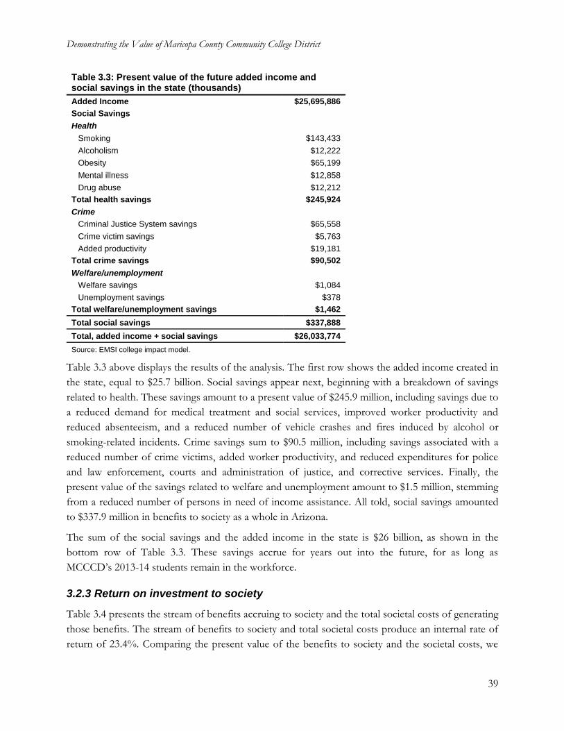
Demonstrating the Value of Maricopa County Community College District
39
Table 3.3: Present value of the future added income and social savings in the state (thousands)
Added Income $25,695,886
Social Savings
Health
Smoking $143,433
Alcoholism $12,222
Obesity $65,199
Mental illness $12,858
Drug abuse $12,212
Total health savings $245,924
Crime
Criminal Justice System savings $65,558
Crime victim savings $5,763
Added productivity $19,181
Total crime savings $90,502
Welfare/unemployment
Welfare savings $1,084
Unemployment savings $378
Total welfare/unemployment savings $1,462
Total social savings $337,888
Total, added income + social savings $26,033,774
Source: EMSI college impact model.
Table 3.3 above displays the results of the analysis. The first row shows the added income created in
the state, equal to $25.7 billion. Social savings appear next, beginning with a breakdown of savings
related to health. These savings amount to a present value of $245.9 million, including savings due to
a reduced demand for medical treatment and social services, improved worker productivity and
reduced absenteeism, and a reduced number of vehicle crashes and fires induced by alcohol or
smoking-related incidents. Crime savings sum to $90.5 million, including savings associated with a
reduced number of crime victims, added worker productivity, and reduced expenditures for police
and law enforcement, courts and administration of justice, and corrective services. Finally, the
present value of the savings related to welfare and unemployment amount to $1.5 million, stemming
from a reduced number of persons in need of income assistance. All told, social savings amounted
to $337.9 million in benefits to society as a whole in Arizona.
The sum of the social savings and the added income in the state is $26 billion, as shown in the
bottom row of Table 3.3. These savings accrue for years out into the future, for as long as
MCCCD’s 2013-14 students remain in the workforce.
3.2.3 Return on investment to society
Table 3.4 presents the stream of benefits accruing to society and the total societal costs of generating
those benefits. The stream of benefits to society and total societal costs produce an internal rate of
return of 23.4%. Comparing the present value of the benefits to society and the societal costs, we
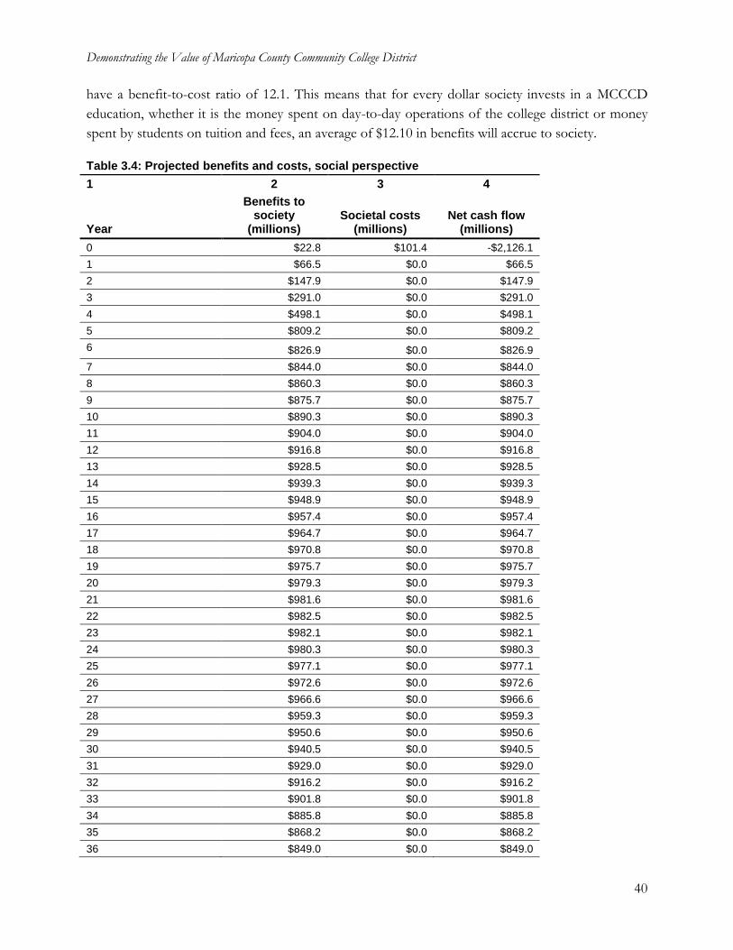
Demonstrating the Value of Maricopa County Community College District
40
have a benefit-to-cost ratio of 12.1. This means that for every dollar society invests in a MCCCD
education, whether it is the money spent on day-to-day operations of the college district or money
spent by students on tuition and fees, an average of $12.10 in benefits will accrue to society.
Table 3.4: Projected benefits and costs, social perspective
1 2 3 4
Year
Benefits to society
(millions) Societal costs
(millions) Net cash flow
(millions)
0 $22.8 $101.4 -$2,126.1
1 $66.5 $0.0 $66.5
2 $147.9 $0.0 $147.9
3 $291.0 $0.0 $291.0
4 $498.1 $0.0 $498.1
5 $809.2 $0.0 $809.2
6 $826.9 $0.0 $826.9
7 $844.0 $0.0 $844.0
8 $860.3 $0.0 $860.3
9 $875.7 $0.0 $875.7
10 $890.3 $0.0 $890.3
11 $904.0 $0.0 $904.0
12 $916.8 $0.0 $916.8
13 $928.5 $0.0 $928.5
14 $939.3 $0.0 $939.3
15 $948.9 $0.0 $948.9
16 $957.4 $0.0 $957.4
17 $964.7 $0.0 $964.7
18 $970.8 $0.0 $970.8
19 $975.7 $0.0 $975.7
20 $979.3 $0.0 $979.3
21 $981.6 $0.0 $981.6
22 $982.5 $0.0 $982.5
23 $982.1 $0.0 $982.1
24 $980.3 $0.0 $980.3
25 $977.1 $0.0 $977.1
26 $972.6 $0.0 $972.6
27 $966.6 $0.0 $966.6
28 $959.3 $0.0 $959.3
29 $950.6 $0.0 $950.6
30 $940.5 $0.0 $940.5
31 $929.0 $0.0 $929.0
32 $916.2 $0.0 $916.2
33 $901.8 $0.0 $901.8
34 $885.8 $0.0 $885.8
35 $868.2 $0.0 $868.2
36 $849.0 $0.0 $849.0
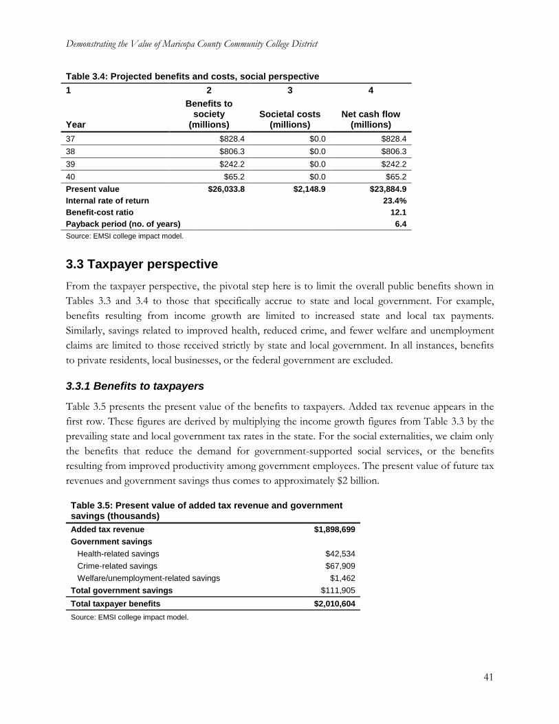
Demonstrating the Value of Maricopa County Community College District
41
Table 3.4: Projected benefits and costs, social perspective
1 2 3 4
Year
Benefits to society
(millions) Societal costs
(millions) Net cash flow
(millions)
37 $828.4 $0.0 $828.4
38 $806.3 $0.0 $806.3
39 $242.2 $0.0 $242.2
40 $65.2 $0.0 $65.2
Present value $26,033.8 $2,148.9 $23,884.9
Internal rate of return 23.4%
Benefit-cost ratio 12.1
Payback period (no. of years) 6.4
Source: EMSI college impact model.
3.3 Taxpayer perspective
From the taxpayer perspective, the pivotal step here is to limit the overall public benefits shown in
Tables 3.3 and 3.4 to those that specifically accrue to state and local government. For example,
benefits resulting from income growth are limited to increased state and local tax payments.
Similarly, savings related to improved health, reduced crime, and fewer welfare and unemployment
claims are limited to those received strictly by state and local government. In all instances, benefits
to private residents, local businesses, or the federal government are excluded.
3.3.1 Benefits to taxpayers
Table 3.5 presents the present value of the benefits to taxpayers. Added tax revenue appears in the
first row. These figures are derived by multiplying the income growth figures from Table 3.3 by the
prevailing state and local government tax rates in the state. For the social externalities, we claim only
the benefits that reduce the demand for government-supported social services, or the benefits
resulting from improved productivity among government employees. The present value of future tax
revenues and government savings thus comes to approximately $2 billion.
Table 3.5: Present value of added tax revenue and government savings (thousands)
Added tax revenue $1,898,699
Government savings
Health-related savings $42,534
Crime-related savings $67,909
Welfare/unemployment-related savings $1,462
Total government savings $111,905
Total taxpayer benefits $2,010,604
Source: EMSI college impact model.
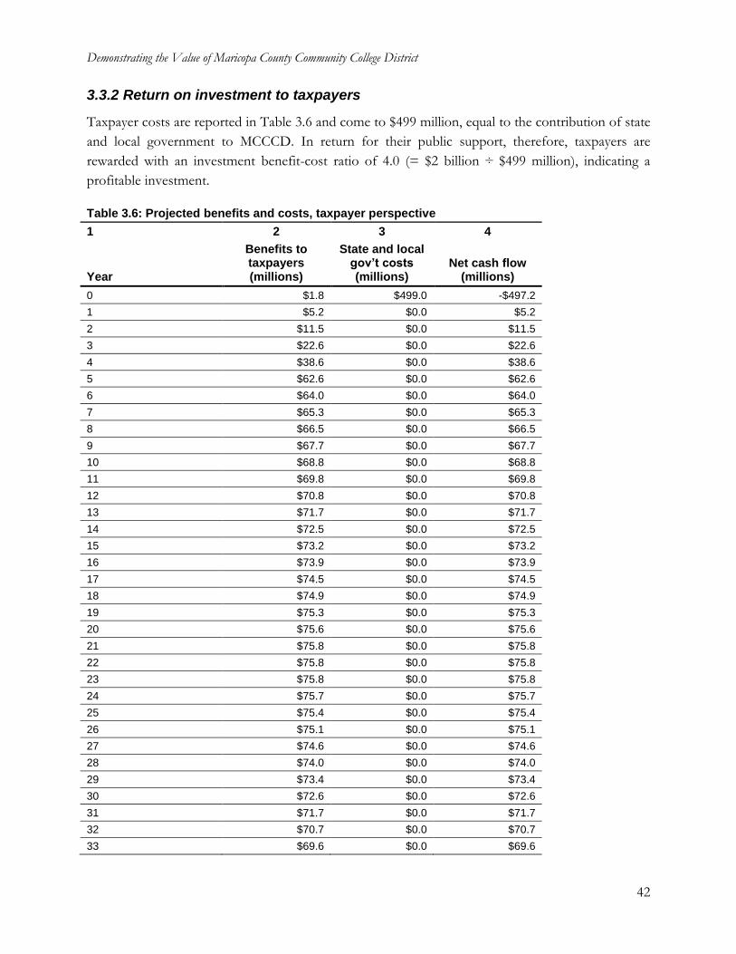
Demonstrating the Value of Maricopa County Community College District
42
3.3.2 Return on investment to taxpayers
Taxpayer costs are reported in Table 3.6 and come to $499 million, equal to the contribution of state
and local government to MCCCD. In return for their public support, therefore, taxpayers are
rewarded with an investment benefit-cost ratio of 4.0 (= $2 billion ÷ $499 million), indicating a
profitable investment.
Table 3.6: Projected benefits and costs, taxpayer perspective
1 2 3 4
Year
Benefits to taxpayers (millions)
State and local gov’t costs (millions)
Net cash flow (millions)
0 $1.8 $499.0 -$497.2
1 $5.2 $0.0 $5.2
2 $11.5 $0.0 $11.5
3 $22.6 $0.0 $22.6
4 $38.6 $0.0 $38.6
5 $62.6 $0.0 $62.6
6 $64.0 $0.0 $64.0
7 $65.3 $0.0 $65.3
8 $66.5 $0.0 $66.5
9 $67.7 $0.0 $67.7
10 $68.8 $0.0 $68.8
11 $69.8 $0.0 $69.8
12 $70.8 $0.0 $70.8
13 $71.7 $0.0 $71.7
14 $72.5 $0.0 $72.5
15 $73.2 $0.0 $73.2
16 $73.9 $0.0 $73.9
17 $74.5 $0.0 $74.5
18 $74.9 $0.0 $74.9
19 $75.3 $0.0 $75.3
20 $75.6 $0.0 $75.6
21 $75.8 $0.0 $75.8
22 $75.8 $0.0 $75.8
23 $75.8 $0.0 $75.8
24 $75.7 $0.0 $75.7
25 $75.4 $0.0 $75.4
26 $75.1 $0.0 $75.1
27 $74.6 $0.0 $74.6
28 $74.0 $0.0 $74.0
29 $73.4 $0.0 $73.4
30 $72.6 $0.0 $72.6
31 $71.7 $0.0 $71.7
32 $70.7 $0.0 $70.7
33 $69.6 $0.0 $69.6
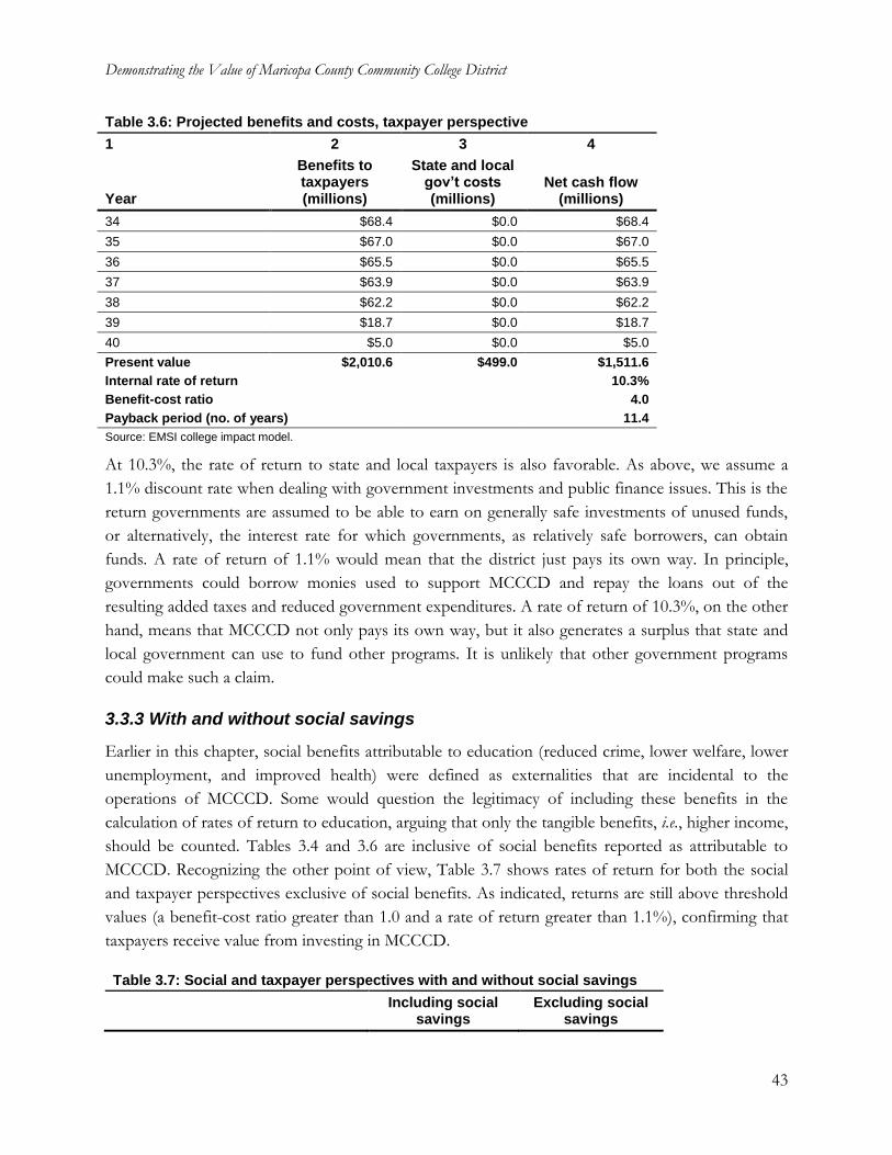
Demonstrating the Value of Maricopa County Community College District
43
Table 3.6: Projected benefits and costs, taxpayer perspective
1 2 3 4
Year
Benefits to taxpayers (millions)
State and local gov’t costs (millions)
Net cash flow (millions)
34 $68.4 $0.0 $68.4
35 $67.0 $0.0 $67.0
36 $65.5 $0.0 $65.5
37 $63.9 $0.0 $63.9
38 $62.2 $0.0 $62.2
39 $18.7 $0.0 $18.7
40 $5.0 $0.0 $5.0
Present value $2,010.6 $499.0 $1,511.6
Internal rate of return 10.3%
Benefit-cost ratio 4.0
Payback period (no. of years) 11.4
Source: EMSI college impact model.
At 10.3%, the rate of return to state and local taxpayers is also favorable. As above, we assume a
1.1% discount rate when dealing with government investments and public finance issues. This is the
return governments are assumed to be able to earn on generally safe investments of unused funds,
or alternatively, the interest rate for which governments, as relatively safe borrowers, can obtain
funds. A rate of return of 1.1% would mean that the district just pays its own way. In principle,
governments could borrow monies used to support MCCCD and repay the loans out of the
resulting added taxes and reduced government expenditures. A rate of return of 10.3%, on the other
hand, means that MCCCD not only pays its own way, but it also generates a surplus that state and
local government can use to fund other programs. It is unlikely that other government programs
could make such a claim.
3.3.3 With and without social savings
Earlier in this chapter, social benefits attributable to education (reduced crime, lower welfare, lower
unemployment, and improved health) were defined as externalities that are incidental to the
operations of MCCCD. Some would question the legitimacy of including these benefits in the
calculation of rates of return to education, arguing that only the tangible benefits, i.e., higher income,
should be counted. Tables 3.4 and 3.6 are inclusive of social benefits reported as attributable to
MCCCD. Recognizing the other point of view, Table 3.7 shows rates of return for both the social
and taxpayer perspectives exclusive of social benefits. As indicated, returns are still above threshold
values (a benefit-cost ratio greater than 1.0 and a rate of return greater than 1.1%), confirming that
taxpayers receive value from investing in MCCCD.
Table 3.7: Social and taxpayer perspectives with and without social savings
Including social
savings Excluding social
savings
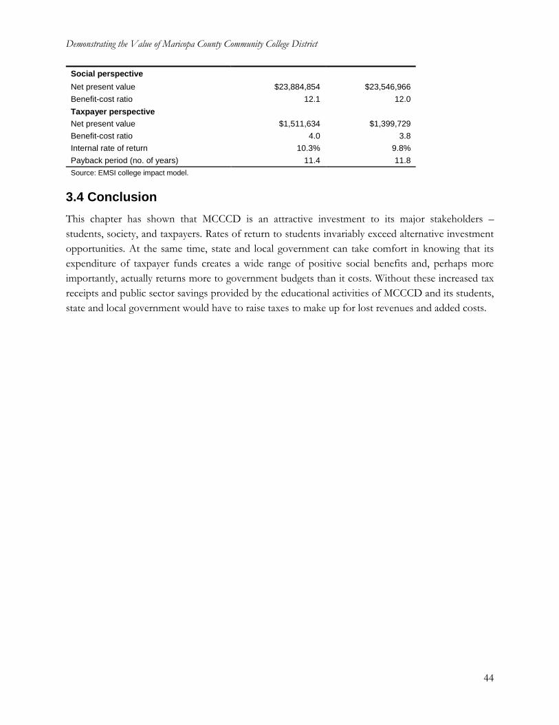
Demonstrating the Value of Maricopa County Community College District
44
Social perspective
Net present value $23,884,854 $23,546,966
Benefit-cost ratio 12.1 12.0
Taxpayer perspective
Net present value $1,511,634 $1,399,729
Benefit-cost ratio 4.0 3.8
Internal rate of return 10.3% 9.8%
Payback period (no. of years) 11.4 11.8
Source: EMSI college impact model.
3.4 Conclusion
This chapter has shown that MCCCD is an attractive investment to its major stakeholders –
students, society, and taxpayers. Rates of return to students invariably exceed alternative investment
opportunities. At the same time, state and local government can take comfort in knowing that its
expenditure of taxpayer funds creates a wide range of positive social benefits and, perhaps more
importantly, actually returns more to government budgets than it costs. Without these increased tax
receipts and public sector savings provided by the educational activities of MCCCD and its students,
state and local government would have to raise taxes to make up for lost revenues and added costs.
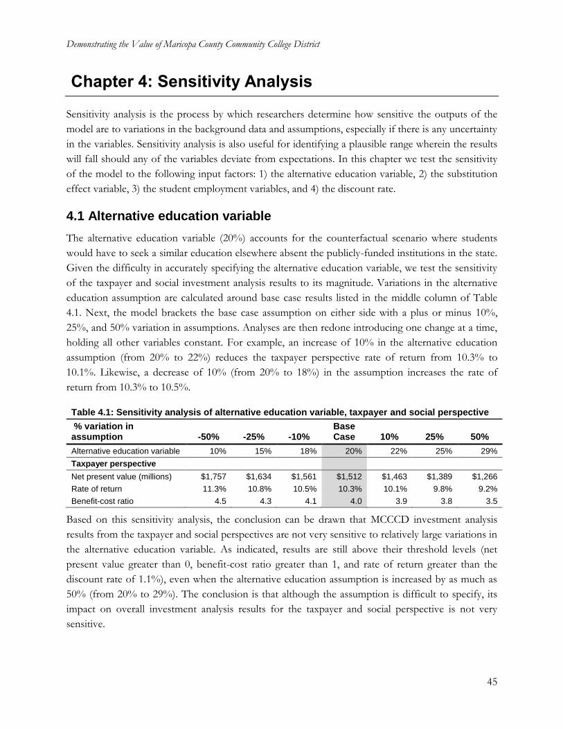
Demonstrating the Value of Maricopa County Community College District
45
Chapter 4: Sensitivity Analysis
Sensitivity analysis is the process by which researchers determine how sensitive the outputs of the
model are to variations in the background data and assumptions, especially if there is any uncertainty
in the variables. Sensitivity analysis is also useful for identifying a plausible range wherein the results
will fall should any of the variables deviate from expectations. In this chapter we test the sensitivity
of the model to the following input factors: 1) the alternative education variable, 2) the substitution
effect variable, 3) the student employment variables, and 4) the discount rate.
4.1 Alternative education variable
The alternative education variable (20%) accounts for the counterfactual scenario where students
would have to seek a similar education elsewhere absent the publicly-funded institutions in the state.
Given the difficulty in accurately specifying the alternative education variable, we test the sensitivity
of the taxpayer and social investment analysis results to its magnitude. Variations in the alternative
education assumption are calculated around base case results listed in the middle column of Table
4.1. Next, the model brackets the base case assumption on either side with a plus or minus 10%,
25%, and 50% variation in assumptions. Analyses are then redone introducing one change at a time,
holding all other variables constant. For example, an increase of 10% in the alternative education
assumption (from 20% to 22%) reduces the taxpayer perspective rate of return from 10.3% to
10.1%. Likewise, a decrease of 10% (from 20% to 18%) in the assumption increases the rate of
return from 10.3% to 10.5%.
Table 4.1: Sensitivity analysis of alternative education variable, taxpayer and social perspective
% variation in assumption -50% -25% -10%
Base Case 10% 25% 50%
Alternative education variable 10% 15% 18% 20% 22% 25% 29%
Taxpayer perspective
Net present value (millions) $1,757 $1,634 $1,561 $1,512 $1,463 $1,389 $1,266
Rate of return 11.3% 10.8% 10.5% 10.3% 10.1% 9.8% 9.2%
Benefit-cost ratio 4.5 4.3 4.1 4.0 3.9 3.8 3.5
Based on this sensitivity analysis, the conclusion can be drawn that MCCCD investment analysis
results from the taxpayer and social perspectives are not very sensitive to relatively large variations in
the alternative education variable. As indicated, results are still above their threshold levels (net
present value greater than 0, benefit-cost ratio greater than 1, and rate of return greater than the
discount rate of 1.1%), even when the alternative education assumption is increased by as much as
50% (from 20% to 29%). The conclusion is that although the assumption is difficult to specify, its
impact on overall investment analysis results for the taxpayer and social perspective is not very
sensitive.
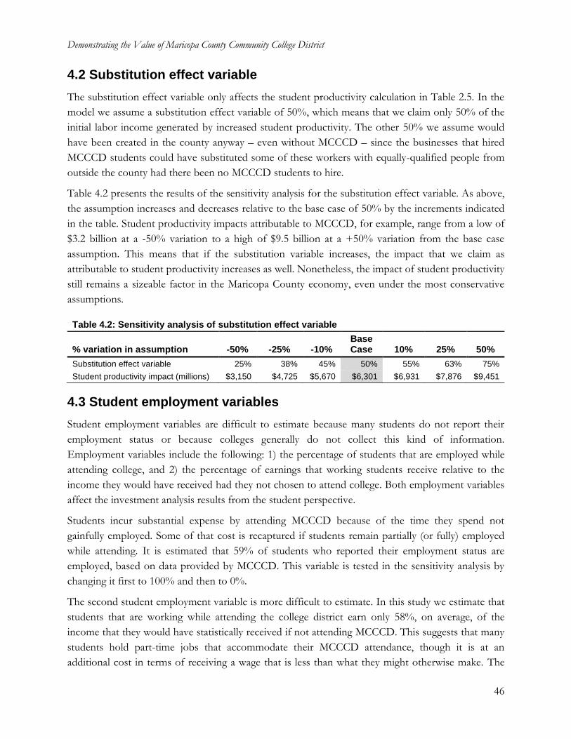
Demonstrating the Value of Maricopa County Community College District
46
4.2 Substitution effect variable
The substitution effect variable only affects the student productivity calculation in Table 2.5. In the
model we assume a substitution effect variable of 50%, which means that we claim only 50% of the
initial labor income generated by increased student productivity. The other 50% we assume would
have been created in the county anyway – even without MCCCD – since the businesses that hired
MCCCD students could have substituted some of these workers with equally-qualified people from
outside the county had there been no MCCCD students to hire.
Table 4.2 presents the results of the sensitivity analysis for the substitution effect variable. As above,
the assumption increases and decreases relative to the base case of 50% by the increments indicated
in the table. Student productivity impacts attributable to MCCCD, for example, range from a low of
$3.2 billion at a -50% variation to a high of $9.5 billion at a +50% variation from the base case
assumption. This means that if the substitution variable increases, the impact that we claim as
attributable to student productivity increases as well. Nonetheless, the impact of student productivity
still remains a sizeable factor in the Maricopa County economy, even under the most conservative
assumptions.
Table 4.2: Sensitivity analysis of substitution effect variable
% variation in assumption -50% -25% -10% Base Case 10% 25% 50%
Substitution effect variable 25% 38% 45% 50% 55% 63% 75%
Student productivity impact (millions) $3,150 $4,725 $5,670 $6,301 $6,931 $7,876 $9,451
4.3 Student employment variables
Student employment variables are difficult to estimate because many students do not report their
employment status or because colleges generally do not collect this kind of information.
Employment variables include the following: 1) the percentage of students that are employed while
attending college, and 2) the percentage of earnings that working students receive relative to the
income they would have received had they not chosen to attend college. Both employment variables
affect the investment analysis results from the student perspective.
Students incur substantial expense by attending MCCCD because of the time they spend not
gainfully employed. Some of that cost is recaptured if students remain partially (or fully) employed
while attending. It is estimated that 59% of students who reported their employment status are
employed, based on data provided by MCCCD. This variable is tested in the sensitivity analysis by
changing it first to 100% and then to 0%.
The second student employment variable is more difficult to estimate. In this study we estimate that
students that are working while attending the college district earn only 58%, on average, of the
income that they would have statistically received if not attending MCCCD. This suggests that many
students hold part-time jobs that accommodate their MCCCD attendance, though it is at an
additional cost in terms of receiving a wage that is less than what they might otherwise make. The
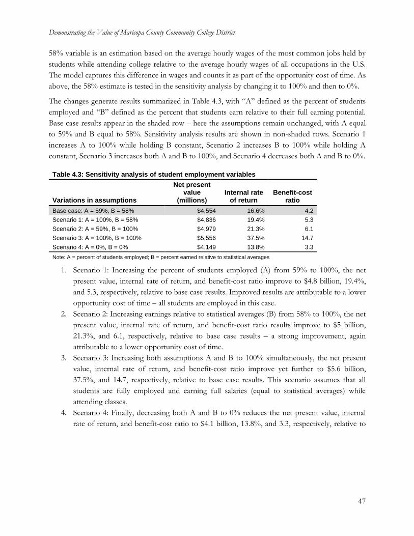
Demonstrating the Value of Maricopa County Community College District
47
58% variable is an estimation based on the average hourly wages of the most common jobs held by
students while attending college relative to the average hourly wages of all occupations in the U.S.
The model captures this difference in wages and counts it as part of the opportunity cost of time. As
above, the 58% estimate is tested in the sensitivity analysis by changing it to 100% and then to 0%.
The changes generate results summarized in Table 4.3, with “A” defined as the percent of students
employed and “B” defined as the percent that students earn relative to their full earning potential.
Base case results appear in the shaded row – here the assumptions remain unchanged, with A equal
to 59% and B equal to 58%. Sensitivity analysis results are shown in non-shaded rows. Scenario 1
increases A to 100% while holding B constant, Scenario 2 increases B to 100% while holding A
constant, Scenario 3 increases both A and B to 100%, and Scenario 4 decreases both A and B to 0%.
Table 4.3: Sensitivity analysis of student employment variables
Variations in assumptions
Net present value
(millions) Internal rate
of return Benefit-cost
ratio
Base case: A = 59%, B = 58% $4,554 16.6% 4.2
Scenario 1: A = 100%, B = 58% $4,836 19.4% 5.3
Scenario 2: A = 59%, B = 100% $4,979 21.3% 6.1
Scenario 3: A = 100%, B = 100% $5,556 37.5% 14.7
Scenario 4: A = 0%, B = 0% $4,149 13.8% 3.3
Note: A = percent of students employed; B = percent earned relative to statistical averages
1. Scenario 1: Increasing the percent of students employed (A) from 59% to 100%, the net
present value, internal rate of return, and benefit-cost ratio improve to $4.8 billion, 19.4%,
and 5.3, respectively, relative to base case results. Improved results are attributable to a lower
opportunity cost of time – all students are employed in this case.
2. Scenario 2: Increasing earnings relative to statistical averages (B) from 58% to 100%, the net
present value, internal rate of return, and benefit-cost ratio results improve to $5 billion,
21.3%, and 6.1, respectively, relative to base case results – a strong improvement, again
attributable to a lower opportunity cost of time.
3. Scenario 3: Increasing both assumptions A and B to 100% simultaneously, the net present
value, internal rate of return, and benefit-cost ratio improve yet further to $5.6 billion,
37.5%, and 14.7, respectively, relative to base case results. This scenario assumes that all
students are fully employed and earning full salaries (equal to statistical averages) while
attending classes.
4. Scenario 4: Finally, decreasing both A and B to 0% reduces the net present value, internal
rate of return, and benefit-cost ratio to $4.1 billion, 13.8%, and 3.3, respectively, relative to
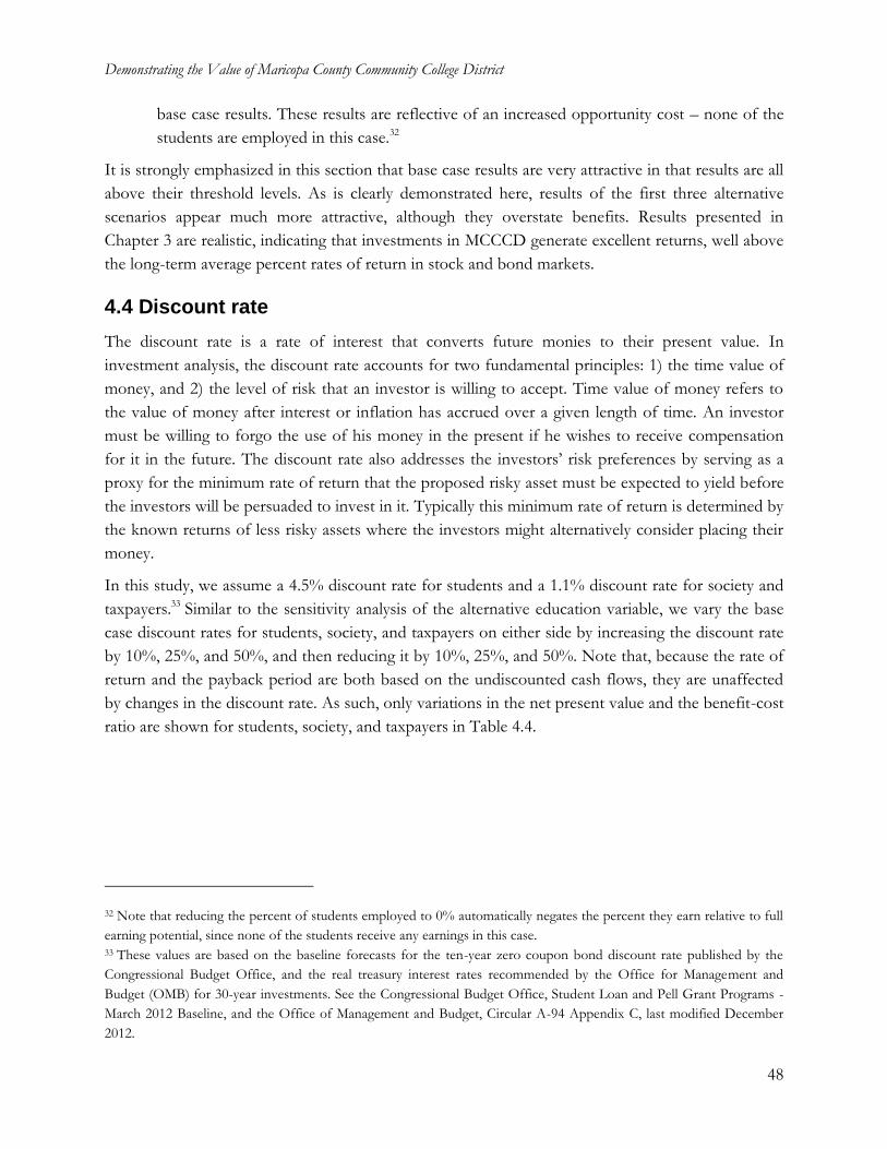
Demonstrating the Value of Maricopa County Community College District
48
base case results. These results are reflective of an increased opportunity cost – none of the
students are employed in this case.32
It is strongly emphasized in this section that base case results are very attractive in that results are all
above their threshold levels. As is clearly demonstrated here, results of the first three alternative
scenarios appear much more attractive, although they overstate benefits. Results presented in
Chapter 3 are realistic, indicating that investments in MCCCD generate excellent returns, well above
the long-term average percent rates of return in stock and bond markets.
4.4 Discount rate
The discount rate is a rate of interest that converts future monies to their present value. In
investment analysis, the discount rate accounts for two fundamental principles: 1) the time value of
money, and 2) the level of risk that an investor is willing to accept. Time value of money refers to
the value of money after interest or inflation has accrued over a given length of time. An investor
must be willing to forgo the use of his money in the present if he wishes to receive compensation
for it in the future. The discount rate also addresses the investors’ risk preferences by serving as a
proxy for the minimum rate of return that the proposed risky asset must be expected to yield before
the investors will be persuaded to invest in it. Typically this minimum rate of return is determined by
the known returns of less risky assets where the investors might alternatively consider placing their
money.
In this study, we assume a 4.5% discount rate for students and a 1.1% discount rate for society and
taxpayers.33 Similar to the sensitivity analysis of the alternative education variable, we vary the base
case discount rates for students, society, and taxpayers on either side by increasing the discount rate
by 10%, 25%, and 50%, and then reducing it by 10%, 25%, and 50%. Note that, because the rate of
return and the payback period are both based on the undiscounted cash flows, they are unaffected
by changes in the discount rate. As such, only variations in the net present value and the benefit-cost
ratio are shown for students, society, and taxpayers in Table 4.4.
32 Note that reducing the percent of students employed to 0% automatically negates the percent they earn relative to full
earning potential, since none of the students receive any earnings in this case. 33 These values are based on the baseline forecasts for the ten-year zero coupon bond discount rate published by the
Congressional Budget Office, and the real treasury interest rates recommended by the Office for Management and
Budget (OMB) for 30-year investments. See the Congressional Budget Office, Student Loan and Pell Grant Programs -
March 2012 Baseline, and the Office of Management and Budget, Circular A-94 Appendix C, last modified December
2012.
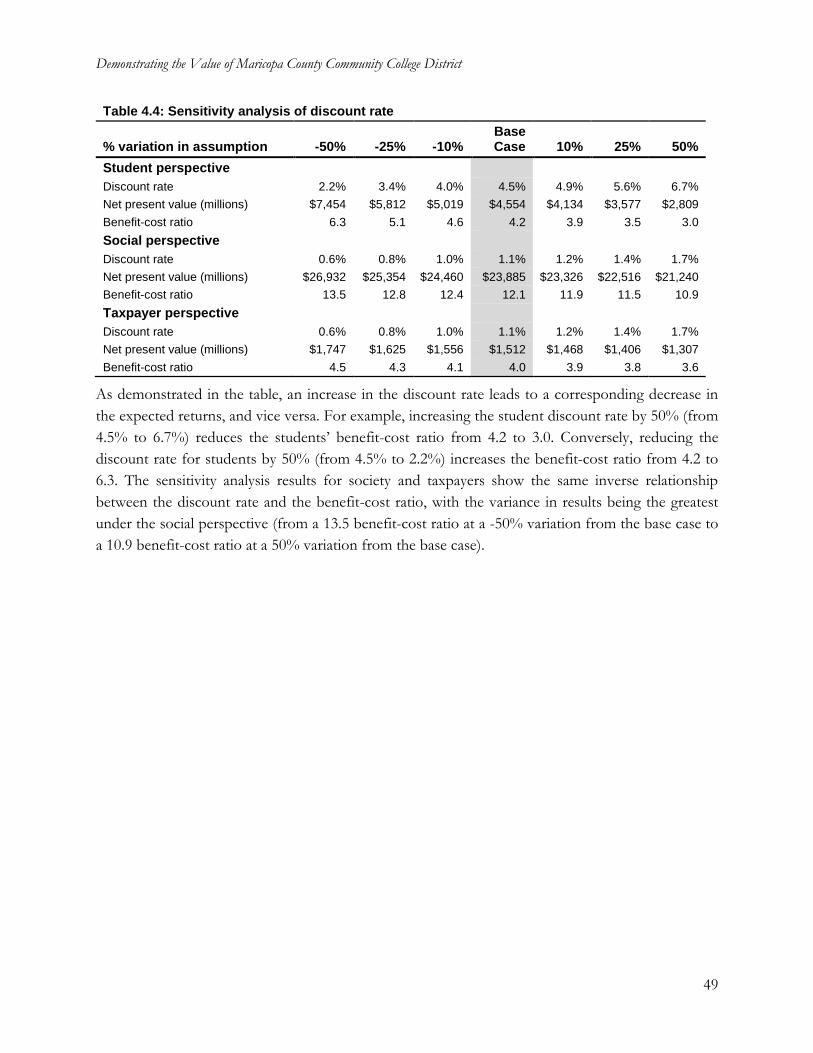
Demonstrating the Value of Maricopa County Community College District
49
Table 4.4: Sensitivity analysis of discount rate
% variation in assumption -50% -25% -10% Base Case 10% 25% 50%
Student perspective
Discount rate 2.2% 3.4% 4.0% 4.5% 4.9% 5.6% 6.7%
Net present value (millions) $7,454 $5,812 $5,019 $4,554 $4,134 $3,577 $2,809
Benefit-cost ratio 6.3 5.1 4.6 4.2 3.9 3.5 3.0
Social perspective
Discount rate 0.6% 0.8% 1.0% 1.1% 1.2% 1.4% 1.7%
Net present value (millions) $26,932 $25,354 $24,460 $23,885 $23,326 $22,516 $21,240
Benefit-cost ratio 13.5 12.8 12.4 12.1 11.9 11.5 10.9
Taxpayer perspective
Discount rate 0.6% 0.8% 1.0% 1.1% 1.2% 1.4% 1.7%
Net present value (millions) $1,747 $1,625 $1,556 $1,512 $1,468 $1,406 $1,307
Benefit-cost ratio 4.5 4.3 4.1 4.0 3.9 3.8 3.6
As demonstrated in the table, an increase in the discount rate leads to a corresponding decrease in
the expected returns, and vice versa. For example, increasing the student discount rate by 50% (from
4.5% to 6.7%) reduces the students’ benefit-cost ratio from 4.2 to 3.0. Conversely, reducing the
discount rate for students by 50% (from 4.5% to 2.2%) increases the benefit-cost ratio from 4.2 to
6.3. The sensitivity analysis results for society and taxpayers show the same inverse relationship
between the discount rate and the benefit-cost ratio, with the variance in results being the greatest
under the social perspective (from a 13.5 benefit-cost ratio at a -50% variation from the base case to
a 10.9 benefit-cost ratio at a 50% variation from the base case).
Demonstrating the Value of Maricopa County Community College District
50
Appendix 1: Resources and References
Administration for Children and Families. Characteristics and Financial Circumstances of TANF
Recipients, Fiscal Year 2010. August 2012. Accessed July 2013.
http://www.acf.hhs.gov/sites/default/files/ofa/appendix_ys_final.pdf.
Administration for Children and Families. “Fiscal Year 2011 TANF Financial Data.” Office of
Family Assistance, TANF Financial Data. Updated August 2012. Accessed August 2013.
http://www.acf.hhs.gov/programs/ofa/resource/tanf-financial-data-fy-2011.
American Automobile Association. “AAA Average Costs Per Mile” in “Your Driving Costs.” AAA
Association Communication: 2012. Accessed May 2012. http://newsroom.aaa.com/wp-
content/uploads/2012/04/YourDrivingCosts2012.pdf.
American Community Survey. “Commuting in the United States: 2009” in “American Community
Survey Reports.” U.S. Department of Commerce Economics and Statistics Administration,
September 2011.
Baryla, Edward and Douglas Dotterweich. “Student Migration: Do Significant Factors Vary by
Region?” Education Economics 9, no. 3 (2001).
Becker, Gary S. Human Capital: A Theoretical and Empirical Analysis, with Special Reference to Education.
New York: Columbia College Press for NBER, 1964.
Bilkic, Natasa, Thomas Gries, and Margarethe Pilichowski. “Stay in school or start working? – The
human capital investment decision under uncertainty and irreversibility.” Labour Economics 19,
no. 5 (October 2012): 706-717.
Bouchery, Ellen, Carol Simon, and Hendrick Harwood. “Economic Costs of Excessive Alcohol
Consumption in the United States, 2006.” The Lewin Group, February 2013. Report prepared
for the Centers for Disease Control and Prevention and the National Foundation for the
Centers for Disease Control and Prevention. Accessed August 2013.
http://www.lewin.com/~/media/Lewin/Site_Sections/Publications/CDC_Report_Rev.pdf.
Bureau of Justice Statistics. “Appendix Table 1 - Prisoners under the jurisdiction of state or federal
correctional authorities, by jurisdiction, December 31, 2000, 2008, and 2009.” in “Prisoners in
2009 (revised).” NCJ 231675, December 2010. Revised October 2011. Accessed July 2013.
http://www.bjs.gov/content/pub/pdf/p09.pdf.
Bureau of Labor Statistics. “Charts by Topic: Leisure and sports activities.” American Time Use
Survey. Last modified November 2012. Accessed July 2013.
http://www.bls.gov/TUS/CHARTS/LEISURE.HTM.
Bureau of Labor Statistics. Consumer Price Index. Accessed January 2013.
ftp://ftp.bls.gov/pub/special.requests/cpi/cpiai.txt.
Demonstrating the Value of Maricopa County Community College District
51
Bureau of Labor Statistics. “Earnings and unemployment rates by educational attainment.” BLS
Employment Projections. Last modified May 2013. Accessed July 2013.
http://www.bls.gov/emp/ep_chart_001.htm.
Bureau of Labor Statistics. “May 2012 National Occupational Employment and Wage Estimates
United States.” Occupational Employment Statistics. Accessed July 2013.
http://www.bls.gov/oes/current/oes_nat.htm.
Bureau of Labor Statistics. “Table 7. Employment status of the civilian noninstitutional population
25 years and over by educational attainment, sex, race, and Hispanic or Latino ethnicity.”
Current Population Survey, Labor Force Statistics. Accessed August 2013.
http://www.bls.gov/cps/cpsaat07.pdf.
Bureau of Labor Statistics. “Table A-10. Unemployment rates by age, sex, and marital status,
seasonally adjusted.” Labor Force Statistics from the Current Population Survey. Last
modified July 2013. Accessed July 2013. http://www.bls.gov/web/empsit/cpseea10.htm.
Buss, Christian, Jeffrey Parker, and Jon Rivenburg. “Cost, quality and enrollment demand at liberal
arts colleges”. Economics of Education Review 23, no.1 (February 2004): 57-65.
Card, David. “The causal effect of education on earnings.” Handbook of Labor Economics 3 (1999):
1801-1863.
Carson, Ann E. and Daniela Golinelli. “Table 1: Prisoners under the jurisdiction of state or federal
correctional authorities, December 31, 2002–2012” in “Prisoners in 2012 - Advance Counts.”
Bureau of Justice Statistics, July 2013, NCJ 242467. Accessed August 2013.
http://www.bjs.gov/content/pub/pdf/p12ac.pdf.
Center on Budget and Policy Priorities. “Policy Basics - How many weeks of unemployment are
available?” Updated August 26, 2013. Accessed August 27, 2013.
http://www.cbpp.org/files/PolicyBasics_UI_Weeks.pdf.
Centers for Disease Control and Prevention. “Adult Obesity Facts.” Overweight and Obesity.
Accessed August 2013. http://www.cdc.gov/obesity/data/adult.html#Prevalence.
Centers for Disease Control and Prevention. “Adults who are current smokers” in “Tobacco Use -
2011.” Behavioral Risk Factor Surveillance System Prevalence and Trends Data. Accessed
August 2013.
http://apps.nccd.cdc.gov/brfss/list.asp?cat=TU&yr=2011&qkey=8161&state=All.
Centers for Disease Control and Prevention. “Heavy drinkers (adult men having more than two
drinks per day and adult women having more than one drink per day)” in “Alcohol
Consumption - 2012.” Behavioral Risk Factor Surveillance System Prevalence and Trends
Data. Accessed August 2013.
http://apps.nccd.cdc.gov/brfss/list.asp?cat=AC&yr=2012&qkey=8381&state=All.
Demonstrating the Value of Maricopa County Community College District
52
Centers for Disease Control and Prevention. “Table 1. Number of respondents to a question about
mental health and percentage who self-reported frequent mental distress (FMD), by
demographic characteristics – United States, Behavioral Risk Factor Surveillance System,
1993-1996” in “Self-Reported Frequent Mental Distress Among Adults – United States, 1993-
1996.” Morbidity and Mortality Weekly Report 47, no. 16 (May 1998): 325-331.
Centers for Disease Control and Prevention. “Table 3: Prevalence of current depression among
adults aged ≥18 years, by sociodemographic characteristics and year – Behavioral Risk Factor
Surveillance System, multiple states, 2006 and 2008” in “Mental Illness Surveillance Among
Adults in the United States.” Morbidity and Mortality Weekly Report 60 supplement (September
2011): 17.
Centers for Disease Control and Prevention. “Table 61. Age-adjusted prevalence of current cigarette
smoking among adults aged 25 and over, by sex, race, and education level: United States,
selected years 1974-2011.” National Health Interview Survey, 2011. Accessed August 2013.
http://www.cdc.gov/nchs/data/hus/2011/061.pdf.
College Board. “Figure 1: Average Estimated Full-Time Undergraduate Budgets, 2012-13
(Enrollment-Weighted)” in “Average Estimated Undergraduate Budgets, 2012-13.” The
College Board, Annual Survey of Colleges. Accessed August 2013.
http://trends.collegeboard.org/college-pricing/figures-tables/average-estimated-
undergraduate-budgets-2012-13.
Congressional Budget Office. Student Loan and Pell Grant Programs - March 2012 Baseline.
Congressional Budget Office Publications. Last modified March 13, 2012. Accessed July 2013.
http://www.cbo.gov/sites/default/files/cbofiles/attachments/43054_StudentLoanPellGrant
Programs.pdf.
Criminal Justice Expenditure and Employment Extracts Program (CJEE). “Table 4. Justice system
expenditure by character, state and type of government, fiscal year 2009 (preliminary).” Justice
Expenditure and Employment Extracts 2009 (preliminary), NCJ 237913. Accessed July 2013.
http://bjs.ojp.usdoj.gov/index.cfm?ty=pbdetail&iid=4335.
Dickerson, Andy, and Steven McIntosh. “The Impact of Distance to Nearest Education Institution
on the Post Compulsory Education Participation Decision.” Urban Studies 50, no. 4 (2013):
742-758.
Dynarski, Susan M. “Does Aid Matter? Measuring the Effect of Student Aid on College Attendance
and Completion.” American Economic Review 93, no. 1 (2003): 279-288.
Economic Modeling Specialists, Intl. Labor market data and software.
www.economicmodeling.com.
Federal Bureau of Investigation, Criminal Justice Information Services Division. “Table 12: Crime
Trends by Population Group, 2009-2010” in “Uniform Crime Reports.” Crime in the United
Demonstrating the Value of Maricopa County Community College District
53
States, Offenses Known to Law Enforcement. Accessed August 2013.
http://www.fbi.gov/about-us/cjis/ucr/crime-in-the-u.s/2010/crime-in-the-u.s.-
2010/offenses-known-to-law-enforcement.
Federal Bureau of Investigation, Criminal Justice Information Services Division. “Table 29:
Estimated Number of Arrests, United States, 2010” in “Uniform Crime Reports.” Crime in
the United States, Persons Arrested. Accessed August 2013. http://www.fbi.gov/about-
us/cjis/ucr/crime-in-the-u.s/2010/crime-in-the-u.s.-2010/tables/10tbl29.xls.
Federal Bureau of Prisons. “Quick Facts About the Bureau of Prisons.” Last updated July 27, 2013.
Accessed August 19, 2013. http://www.bop.gov/news/quick.jsp#1.
Finkelstein, Eric A., Marco da Costa DiBonaventura, Somali M. Burgess, and Brent C. Hale. “The
Costs of Obesity in the Workplace.” Journal of Occupational and Environmental Medicine 52, no. 10
(October 2010): 971-976.
Guerino, Paul, Paige M. Harrison, and William J. Sabol. “Prisoners in 2010.” Bureau of Justice
Statistics, December 2011, NCJ 236096. Accessed August 2013.
http://www.bjs.gov/content/pub/pdf/p10.pdf.
Hamadeh, Mohamad and Roy Khoueiri. “Demand Elasticities for Higher Education in the United
States.” International Journal of Business and Economic Perspectives 5, no. 2 (2010): 60-67.
Harlow, Caroline Wolf. “Table 1. Educational attainment for State and Federal prison inmates, 1997
and 1991, local jail inmates, 1996 and 1989, probationers, 1995, and the general population,
1997” in “Education and Correctional Populations.” Bureau of Justice Statistics Special
Report, January 2003, NCJ 195670. Accessed August 2013.
http://bjs.ojp.usdoj.gov/index.cfm?ty=pbdetail&iid=814.
Henderson, James M. and Richard E. Quandt. Microeconomic Theory: A Mathematical Approach. New
York: McGraw-Hill Book Company, 1971.
Jaeger, David A. and Marianne E. Page. “New Evidence on Sheepskin Effects in the Returns to
Education.” The Review of Economics and Statistics 78, no. 4 (November 1996): 733-740.
Kelchtermans, Stijn and Frank Verboven. “Participation and Study Decisions in a Public System of
Higher Education.” Journal of Applied Econometrics 25, no. 3 (2010): 355-391.
Knapp, Laura G., Janice E. Kelly-Reid, and Scott A. Ginder. “Table 1. Enrollment at all Title IV
institutions, by control of institution, student level, level of institution, attendance status,
gender, and race/ethnicity: United States, fall 2011” in Enrollment in Postsecondary Institutions, Fall
2011; Financial Statistics, Fiscal Year 2011; and Graduation Rates, Selected Cohorts, 2003-2008.
Washington, DC: National Center for Education Statistics, December 2012. Accessed July
2013. http://nces.ed.gov/pubs2012/2012174rev.pdf.
Leigh, Andrew and Chris Ryan. “Estimating returns to education using different natural experiments
techniques.” Economics of Education Review 27 (2008): 149-160.
Demonstrating the Value of Maricopa County Community College District
54
Leonesio, Michael V. “The Economics of Retirement: A Nontechnical Guide.” Social Security Bulletin
59 no. 4 (Winter 1996): 29-50.
McCollister, Kathryn E., Michael T. French, and Hai Fang. “The Cost of Crime to Society: New
Crime-Specific Estimates for Policy and Program Evaluation.” Drug and Alcohol Dependence 108
no.1-2 (April 1, 2010): 98-109. Accessed August 2013.
http://www.ncbi.nlm.nih.gov/pmc/articles/PMC2835847/.
Mincer, Jacob. “Investment in Human Capital and Personal Income Distribution.” Journal of Political
Economy 66, no. 4 (August 1958): 281–302.
Mincer, Jacob. Schooling, Experience and Earnings. New York: National Bureau of Economic Research,
1974.
Minton, Todd. “Table 1: Inmates confined in local jails at midyear, average daily population, and
incarceration rates, 2000–2012” in “Jail Inmates at Midyear 2012 - Statistical Tables.” Bureau
of Justice Statistics, May 2013, NCJ 241264. Accessed August 2013.
www.bjs.gov/content/pub/pdf/jim12st.pdf.
Morgan, James N. and Edward H. Robb. “The impact of age upon interregional migration.” The
Annals of Regional Science 15, no. 3 (November 1981): 31-45.
National Center for Education Statistics. Digest of Education Statistics: 2011. Accessed July 2013.
http://nces.ed.gov/pubsearch/pubsinfo.asp?pubid=2012001.
National Center for Education Statistics, Integrated Post-secondary Education Data System
(IPEDS). http://nces.ed.gov/ipeds/.
National Center for Health Statistics. “Table 74. Healthy weight, overweight, and obesity among
persons 20 years of age and over, by selected characteristics: United States, selected years
1960-1962 through 2007-2010” in Health, United States, 2011 With Special Feature on Socioeconomic
Status and Health. Hyattsville, MD: National Center for Health Statistics, 2012.
National Survey on Drug Use and Health. “Table 1 (REVISED). Serious Mental Illness (SMI) in
Past Year among Persons Aged 18 or Older, by location: Percentages, Annual Averages Based
on 2008 and 2009 NSDUHs” in The NSDUH Mental Illness: State Estimates of Adult Mental
Illness. Center for Behavioral Health Statistics and Quality, Substance Abuse and Mental
Health Services Administration, May 2012.
National Survey on Drug Use and Health. “Table B.1 – Illicit Drug Use in the Past Month, by Age
Group and State: Percentages, Annual Averages Based on 2009 and 2010 NSDUHs” in State
Estimates of Substance Use and Mental Disorders from the 2009-2010 National Surveys on Drug Use and
Health. NSDUH Series H-43, HHS Publication No. (SMA) 12-4703. Rockville, MD: Substance
Abuse and Mental Health Services Administration, 2012.
Office of Management and Budget. Circular A-94 Appendix C. Last modified December 2012.
Accessed July 2013. http://www.whitehouse.gov/omb/circulars_a094/a94_appx-c.
Demonstrating the Value of Maricopa County Community College District
55
Ogden, Cynthia L., Molly M. Lamb, Margaret D. Carroll, and Katherine M. Flegal. “Figure 3.
Prevalence of obesity among adults aged 20 years and over, by education, sex, and race and
ethnicity: United States 2005-2008” in “Obesity and Socioeconomic Status in Adults: United
States 2005-2008.” NCHS data brief no. 50. Hyattsville, MD: National Center for Health
Statistics, 2010.
Polachek, Solomon W. “Earnings Over the Lifecycle: The Mincer Earnings Function and its
Applications.” Foundations and Trends in Microeconomics 4, no. 3 (2008): 165-272.
Polachek, Solomon W. “Mincer’s Overtaking Point and the Lifecycle Earnings Distribution.” Review
of the Economics of the Household 1, no. 4 (December 2003): 273-304.
Ramey, Valerie and Neville Francis. “A Century of Work and Leisure.” American Economic Journal:
Macroeconomics 1, no.2 (2009): 189-224.
Sevilla, Almudena, Jose Ignacio Gimenez-Nadal, and Jonathan I. Gershuny. “Leisure Inequality in
the United States: 1965-2003.” IZA Discussion Paper no. 6708, July 2012.
Substance Abuse and Mental Health Services Administration. “Table 5.7B - Substance Dependence
or Abuse in the Past Year among Persons Aged 26 or Older, by Demographic Characteristics:
Percentages, 2010 and 2011.” SAMSHA, Center for Behavioral Health Statistics and Quality,
National Survey on Drug Use and Health, 2010 and 2011. Accessed August 2013.
http://www.samhsa.gov/data/NSDUH/2011SummNatFindDetTables/NSDUH-
DetTabsPDFWHTML2011/2k11DetailedTabs/Web/HTML/NSDUH-
DetTabsSect5peTabs1to56-2011.htm.
Substance Abuse and Mental Health Services Administration. “Table A.2. Spending by Payer: Levels
and Percent Distribution for Mental Health and Substance Abuse (MHSA), Mental Health
(MH), Substance Abuse (SA), Alcohol Abuse (AA), Drug Abuse (DA), and All-Health, 2005”
in National Expenditures for Mental Health Services & Substance Abuse Treatment, 1986 – 2005.
DHHS Publication No. (SMA) 10-4612. Rockville, MD: Center for Mental Health Services
and Center for Substance Abuse Treatment, Substance Abuse and Mental Health Services
Administration, 2010.
Supplemental Nutrition Assistance Program. “State Activity Report Fiscal Year 2011.” Food and
Nutrition Service, Supplemental Nutrition Assistance Program, Program Accountability and
Administration Division, December 2012. Accessed August 2013.
http://www.fns.usda.gov/snap/qc/pdfs/2011_state_activity.pdf.
Truffer, Christopher J., Sean Keehan, Sheila Smith, Jonathan Cylus, Andrea Sisko, John Poisal,
Joseph Lizonitz, and M. Kent Clemens. “Health Spending Projections Through 2019: The
Recession's Impact Continues.” Health Affairs 29, no. 3 (March 2010): 522-529.
U.S. Census Bureau. “Table 1. Educational Attainment of the Population 18 Years and Over, by
Age, Sex, Race, and Hispanic Origin: 2012.” Educational Attainment in the United States:
Demonstrating the Value of Maricopa County Community College District
56
2012 - Detailed Tables. Accessed August 2013.
http://www.census.gov/hhes/socdemo/education/data/cps/2012/tables.html.
U.S. Census Bureau. “Table 1363. Household Net Savings Rate by Country: 1995 to 2008” in “The
2012 Statistical Abstract International Statistics.” Accessed June 2013.
http://www.census.gov/compendia/statab/2012/tables/12s1363.pdf.
U.S. Census Bureau. “Social Insurance and Human Services” in “The 2012 Statistical Abstract.”
Accessed August 2013.
http://www.census.gov/compendia/statab/cats/social_insurance_human_services.html.
U.S. Census Bureau. “State Characteristics: Vintage 2012.” Population Estimates. Updated June 13,
2013. Accessed August 28, 2013.
http://www.census.gov/popest/data/state/asrh/2012/index.html.
U.S. Department of Health and Human Services. “Chapter II. Indicators of Dependence” in “2008
Indicators of Welfare Dependence.” Annual Report to Congress, 2008. Accessed August
2013. http://aspe.hhs.gov/hsp/indicators08/index.shtml.
U.S. Department of Health and Human Services, Office of Family Assistance. “Table 10:26 -
Temporary Assistance for Needy Families - Active Cases: Percent Distribution of TANF
Adult Recipients by Educational Level, FY 2009” in Temporary Assistance for Needy Families
Program Ninth Report to Congress, 2012. Accessed August 2013.
http://www.acf.hhs.gov/sites/default/files/ofa/ar9appendix.pdf.
U.S. Department of Labor. “Minimum Wage Laws in the States - January 1, 2013.” U.S. Department
of Labor Wage and Hour Division (WHD). Accessed May 2013.
http://www.dol.gov/whd/minwage/america.htm.
U.S. Department of Labor. Unemployment Insurance Data Summary, 4th Quarter 2012. Accessed
July 2013. http://www.ows.doleta.gov/unemploy/content/data.asp.
U.S. Department of the Treasury. “The Economic Costs of Smoking in the United States and the
Benefits of Comprehensive Tobacco Legislation.” Office of Public Affairs Report-3113,
March 1998. Accessed August 2013. http://www.treasury.gov/press-center/press-
releases/Documents/tobacco.pdf.
Willis, Robert J. “Wage Determinants: A Survey and Reinterpretation of Human Capital Earnings
Functions.” In Handbook of Labor Economics, Vol. 1. Edited by Kenneth J. Arrow and Michael
D. Intriligator. Amsterdam: Elsevier Science Publishers, 1986: 525-602.
Witters, Dan, Sengeeta Agrawal, and Diana Liu. “Depression Costs U.S. Workplaces $23 Billion in
Absenteeism.” Gallup-Healthways Well-Being Index, Gallup Wellbeing, July 24, 2013.
Accessed August 28, 2013. http://www.gallup.com/poll/163619/depression-costs-
workplaces-billion-absenteeism.aspx.
Demonstrating the Value of Maricopa County Community College District
57
Appendix 2: Glossary of Terms
Alternative education A “with” and “without” measure of the percent of students who
would still be able to avail themselves of education absent the
publicly-funded educational institutions in the state. An estimate of
10%, for example, means that 10% of students do not depend
directly on the existence of the institution in order to obtain their
education.
Alternative use of funds A measure of how monies that are currently used to fund the
institution might have otherwise been used if the institution did not
exist.
Asset value Capitalized value of a stream of future returns. Asset value measures
what someone would have to pay today for an instrument that
provides the same stream of future revenues.
Attrition rate Rate at which students leave the workforce due to out-migration,
unemployment, retirement, or death.
Benefit-cost ratio Present value of benefits divided by present value of costs. If the
benefit-cost ratio is greater than 1, then benefits exceed costs, and the
investment is feasible.
Credit hour equivalent Credit hour equivalent, or CHE, is defined as 15 contact hours of
education if on a semester system, and 10 contact hours if on a
quarter system. In general, it requires 450 contact hours to complete
one full-time equivalent, or FTE.
Demand Relationship between the market price of education and the volume
of education demanded (expressed in terms of enrollment). The law
of the downward-sloping demand curve is related to the fact that
enrollment increases only if the price (tuition and fees) is lowered, or
conversely, enrollment decreases if price increases.
Discounting Expressing future revenues and costs in present value terms.
Economics Study of the allocation of scarce resources among alternative and
competing ends. Economics is not normative (what ought to be
done), but positive (describes what is, or how people are likely to
behave in response to economic changes).
Elasticity of demand Degree of responsiveness of the quantity of education demanded
(enrollment) to changes in market prices (tuition and fees). If a
Demonstrating the Value of Maricopa County Community College District
58
decrease in fees increases total revenues, demand is elastic. If it
decreases total revenues, demand is inelastic. If total revenues remain
the same, elasticity of demand is unitary.
Externalities Impacts (positive and negative) for which there is no compensation.
Positive externalities of education include improved social behaviors
such as lower crime, reduced welfare and unemployment, and
improved health. Educational institutions do not receive
compensation for these benefits, but benefits still occur because
education is statistically proven to lead to improved social behaviors.
Gross regional product Measure of the final value of all goods and services produced in a
region after netting out the cost of goods used in production.
Alternatively, gross regional product (GRP) equals the combined
incomes of all factors of production, i.e., labor, land and capital.
These include wages, salaries, proprietors’ incomes, profits, rents, and
other. Gross regional product is also sometimes called “value added.”
Initial effect Income generated by the initial injection of monies into the economy
through the payroll of the institution and the higher earnings of its
students.
Input-output analysis Relationship between a given set of demands for final goods and
services and the implied amounts of manufactured inputs, raw
materials, and labor that this requires. In an educational setting, when
institutions pay wages and salaries and spend money for supplies in
the region, they also generate earnings in all sectors of the economy,
thereby increasing the demand for goods and services and jobs.
Moreover, as students enter or rejoin the workforce with higher
skills, they earn higher salaries and wages. In turn, this generates
more consumption and spending in other sectors of the economy.
Internal rate of return Rate of interest which, when used to discount cash flows associated
with investing in education, reduces its net present value to zero (i.e.,
where the present value of revenues accruing from the investment are
just equal to the present value of costs incurred). This, in effect, is the
breakeven rate of return on investment since it shows the highest rate
of interest at which the investment makes neither a profit nor a loss.
Labor income Income which is received as a result of labor, i.e., wages.
Multiplier effect Additional income created in the economy as the institution and its
students spend money in the region. It consists of the income created
by the supply chain of the industries initially affected by the spending
Demonstrating the Value of Maricopa County Community College District
59
of the institution and its students (i.e., the direct effect), income
created by the supply chain of the initial supply chain (i.e., the indirect
effect), and the income created by the increased spending of the
household sector (i.e., the induced effect).
Net cash flow Benefits minus costs, i.e., the sum of revenues accruing from an
investment minus costs incurred.
Net present value Net cash flow discounted to the present. All future cash flows are
collapsed into one number, which, if positive, indicates feasibility.
The result is expressed as a monetary measure.
Non-labor income Income received from investments, such as rent, interest, and
dividends.
Opportunity cost Benefits forgone from alternative B once a decision is made to
allocate resources to alternative A. Or, if individuals choose to attend
college, they forgo earnings that they would have received had they
chosen instead to work full-time. Forgone earnings, therefore, are the
“price tag” of choosing to attend college.
Payback period Length of time required to recover an investment. The shorter the
period, the more attractive the investment. The formula for
computing payback period is:
Payback period = cost of investment/net return per period
Demonstrating the Value of Maricopa County Community College District
60
Appendix 3: EMSI MR-SAM
EMSI’s Multi-Regional Social Accounting Matrix (MR-SAM) represents the flow of all economic
transactions in a given region. It replaces EMSI’s previous input-output (IO) model, which operated
with some 1,100 industries, four layers of government, a single household consumption sector, and
an investment sector. The old IO model was used to simulate the ripple effects (i.e., multipliers) in
the regional economy as a result of industries entering or exiting the region. The SAM model
performs the same tasks as the old IO model, but it also does much more. Along with the same
1,100 industries, government, household and investment sectors embedded in the old IO tool, the
SAM exhibits much more functionality, a greater amount of data, and a higher level of detail on the
demographic and occupational components of jobs (16 demographic cohorts and about 750
occupations are characterized).
This appendix presents a high-level overview of the MR-SAM. Additional detail on the technical
aspects of the model is available upon request; however, we are unable to provide information that
discloses confidential or proprietary methodology.
A3.1 Data sources for the model
The EMSI MR-SAM model relies on a number of internal and external data sources, mostly
compiled by the federal government. What follows is a listing and short explanation of our sources.
The use of these data will be covered in more detail later in this appendix.
EMSI Data are produced from many data sources to produce detailed industry, occupation, and
demographic jobs and earnings data at the local level. This information (especially sales-to-jobs
ratios derived from jobs and earnings-to-sales ratios) is used to help regionalize the national matrices
as well as to disaggregate them into more detailed industries than are normally available.
BEA Make and Use Tables (MUT) are the basis for input-output models in the U.S. The make
table is a matrix that describes the amount of each commodity made by each industry in a given
year. Industries are placed in the rows and commodities in the columns. The use table is a matrix that
describes the amount of each commodity used by each industry in a given year. In the use table,
commodities are placed in the rows and industries in the columns. The BEA produces two different
sets of MUTs, the benchmark and the summary. The benchmark set contains about 500 sectors and
is released every five years, with a five-year lag time (e.g., 2002 benchmark MUTs were released in
2007). The summary set contains about 80 sectors and is released every year, with a two-year lag (e.g.,
2010 summary MUTs were released in late 2011/early 2012). The MUTs are used in the EMSI SAM
model to produce an industry-by-industry matrix describing all industry purchases from all
industries.
BEA Gross Domestic Product by State (GSP) describes gross domestic product from the value
added perspective. Value added is equal to employee compensation, gross operating surplus, and
Demonstrating the Value of Maricopa County Community College District
61
taxes on production and imports, less subsidies. Each of these components is reported for each state
and an aggregate group of industries. This dataset is updated once per year, with a one-year lag. The
EMSI SAM model makes use of this data as a control and pegs certain pieces of the model to values
from this dataset.
BEA National Income and Product Accounts (NIPA) cover a wide variety of economic
measures for the nation, including gross domestic product (GDP), sources of output, and
distribution of income. This dataset is updated periodically throughout the year and can be between
a month and several years old depending on the specific account. NIPA data are used in many of the
EMSI MR-SAM processes as both controls and seeds.
BEA Local Area Income (LPI) encapsulates multiple tables with geographies down to the county
level. The following two tables are specifically used: CA05 (Personal income and earnings by
industry) and CA91 (Gross flow of earnings). CA91 is used when creating the commuting submodel
and CA05 is used in several processes to help with place-of-work and place-of-residence differences,
as well as to calculate personal income, transfers, dividends, interest, and rent.
BLS Consumer Expenditure Survey (CEX) reports on the buying habits of consumers along with
some information as to their income, consumer unit, and demographics. EMSI utilizes this data
heavily in the creation of the national demographic by income type consumption on industries.
Census of Government's (CoG) state and local government finance dataset is used specifically to
aid breaking out state and local data that is reported in the MUTs. This allows EMSI to have unique
production functions for each of its state and local government sectors.
Census' OnTheMap (OTM) is a collection of three datasets for the census block level for multiple
years. Origin-Destination (OD) offers job totals associated with both home census blocks and a
work census block. Residence Area Characteristics (RAC) offers jobs totaled by home census
block. Workplace Area Characteristics (WAC) offers jobs totaled by work census block. All three
of these are used in the commuting submodel to gain better estimates of earnings by industry that
may be counted as commuting. This dataset has holes for specific years and regions. These holes are
filled with Census' Journey-to-Work described later.
Census' Current Population Survey (CPS) is used as the basis for the demographic breakout data
of the MR-SAM model. This set is used to estimate the ratios of demographic cohorts and their
income for the three different income categories (i.e., wages, property income, and transfers).
Census' Journey-to-Work (JtW) is part of the 2000 Census and describes the amount of
commuting jobs between counties. This set is used to fill in the areas where OTM does not have
data.
Census' American Community Survey (ACS) Public Use Microdata Sample (PUMS) is the
replacement for Census' long form and is used by EMSI to fill the holes in the CPS data.
Demonstrating the Value of Maricopa County Community College District
62
Oak Ridge National Lab (ORNL) County-to-County Distance Matrix (Skim Tree) contains a
matrix of distances and network impedances between each county via various modes of
transportation such as highway, railroad, water, and combined highway-rail. Also included in this set
are minimum impedances utilizing the best combination of paths. The ORNL distance matrix is
used in EMSI’s gravitational flows model that estimates the amount of trade between counties in the
country.
A3.2 Overview of the MR-SAM model
EMSI’s multi-regional social accounting matrix (MR-SAM) modeling system is a “comparative
static” type model in the same general class as RIMS II (Bureau of Economic Analysis) and
IMPLAN (Minnesota Implan Group). The MR-SAM model is thus not an “econometric” type
model, the primary example of which is PolicyInsight by REMI. It relies on a matrix representation
of industry-to-industry purchasing patterns originally based on national data which are regionalized
with the use of local data and mathematical manipulation (i.e., non-survey methods). Models of this
type estimate the ripple effects of changes in jobs, earnings, or sales in one or more industries upon
other industries in a region.
The EMSI SAM model shows final equilibrium impacts – that is, the user enters a change that
perturbs the economy and the model shows the changes required to establish a new equilibrium. As
such, it is not a “dynamic” type model that shows year-by-year changes over time (as REMI’s does).
A3.2.1 National SAM
Following standard practice, the SAM model appears as a square matrix, with each row sum exactly
equaling the corresponding column sum. Reflecting its kinship with the standard Leontief input-
output framework, individual SAM elements show accounting flows between row and column
sectors during a chosen base year. Read across rows, SAM entries show the flow of funds into
column accounts (a.k.a., “receipts” or “the appropriation of funds” by those column accounts). Read
down columns, SAM entries show the flow of funds into row accounts (a.k.a., “expenditures” or
“the dispersal of funds” to those row accounts).
The SAM may be broken into three different aggregation layers: broad accounts, sub-accounts, and
detailed accounts. The broad layer is the most aggregate and will be covered first. Broad accounts
cover between one and four sub-accounts, which in turn cover many detailed accounts. This
appendix will not discuss detailed accounts directly because of their number. For example, in the
industry broad account, there are two sub-accounts and over 1,100 detailed accounts.
A3.2.2 Multi-regional aspect of the SAM
Multi-regional (MR) describes a non-survey model that has the ability to analyze the transactions and
ripple effects (i.e., multipliers) of not just a single region, but multiple regions interacting with each
other. Regions in this case are made up of a collection of counties.
Demonstrating the Value of Maricopa County Community College District
63
EMSI’s multi-regional model is built off of gravitational flows, assuming that the larger a county’s
economy, the more influence it will have on the surrounding counties’ purchases and sales. The
equation behind this model is essentially the same that Isaac Newton used to calculate the
gravitational pull between planets and stars. In Newton’s equation, the masses of both objects are
multiplied, then divided by the distance separating them and multiplied by a constant. In EMSI’s
model, the masses are replaced with the supply of a sector for one county and the demand for that
same sector from another county. The distance is replaced with an impedance value that takes into
account the distance, type of roads, rail lines, and other modes of transportation. Once this is
calculated for every county-to-county pair, a set of mathematical operations is performed to make
sure all counties absorb the correct amount of supply from every county and the correct amount of
demand from every county. These operations produce more than 200 million data points.
With the flows finalized, EMSI is able to use industry standard equations to adjust the national SAM
and bring it into focus for the given region or regions. If the model being created is multi-regional,
the amount and kind of transactions that occur between those regions is also calculated.
A3.3 Components of the EMSI SAM model
The EMSI MR-SAM is built from a number of different components that are gathered together to
display information whenever a user selects a region. What follows is a description of each of these
components and how each is created. EMSI’s internally created data are used to a great extent
throughout the processes described below, but its creation is not described in this appendix.
A3.3.1 County earnings distribution matrix
The county earnings distribution matrices describe the earnings spent by every industry on every
occupation for a year – i.e., earnings by occupation. The matrices are built utilizing EMSI’s industry
earnings, occupational average earnings, and staffing patterns.
Each matrix starts with a region’s staffing pattern matrix which is multiplied by the industry jobs
vector. This produces the number of occupational jobs in each industry for the region. Next, the
occupational average hourly earnings per job is multiplied by 2,080 hours, which converts the
average hourly earnings into a yearly estimate. Then the matrix of occupational jobs is multiplied by
the occupational annual earnings per job, converting it into earnings values. Last, all earnings are
adjusted to match the known industry totals. This is a fairly simple process, but one that is very
important. These matrices describe the place-of-work earnings used by the MR-SAM.
A3.3.2 Commuting model
The commuting sub-model is an integral part of EMSI’s MR-SAM model. It allows the regional and
multi-regional models to know what amount of the earnings can be attributed to place-of-residence
vs. place-of-work. The commuting data describe the flow of earnings from any county to any other
county (including within the counties themselves). For this situation, the commuted earnings are not
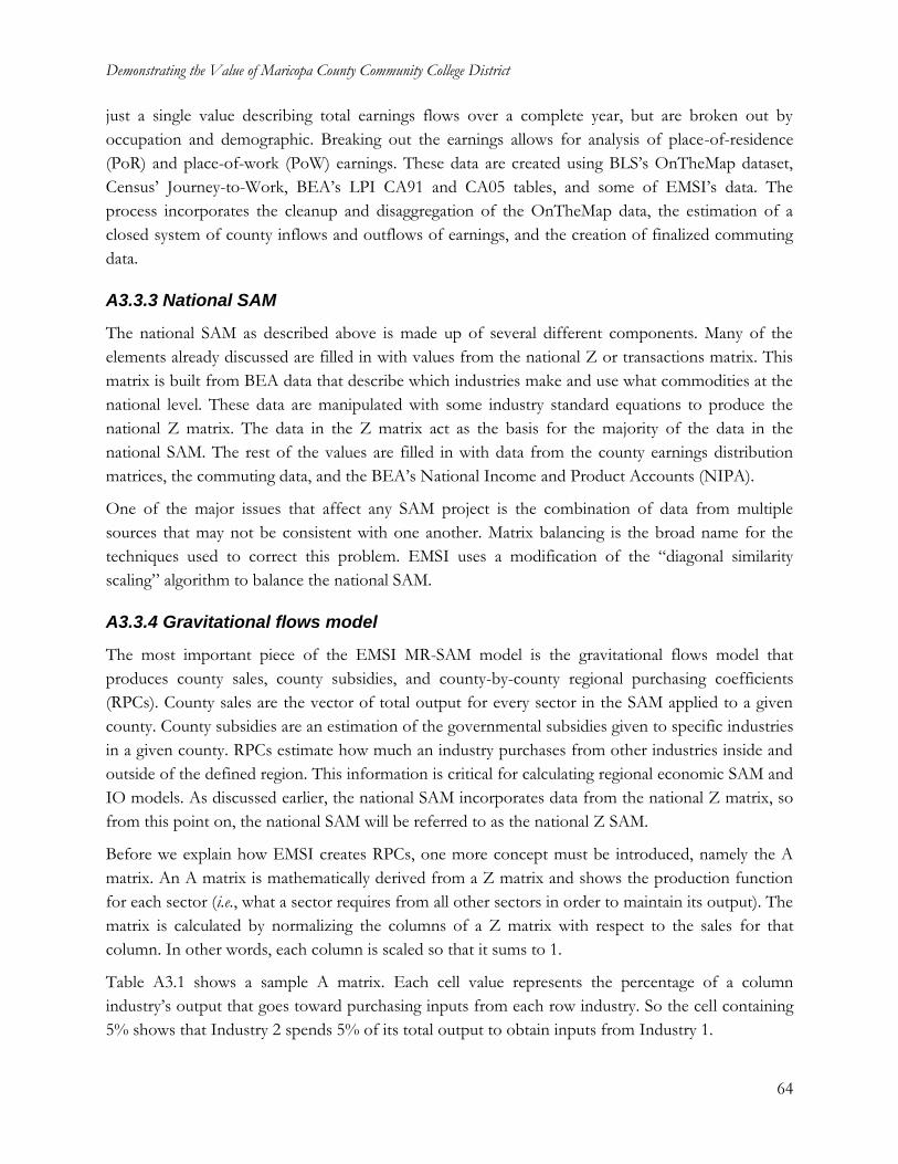
Demonstrating the Value of Maricopa County Community College District
64
just a single value describing total earnings flows over a complete year, but are broken out by
occupation and demographic. Breaking out the earnings allows for analysis of place-of-residence
(PoR) and place-of-work (PoW) earnings. These data are created using BLS’s OnTheMap dataset,
Census’ Journey-to-Work, BEA’s LPI CA91 and CA05 tables, and some of EMSI’s data. The
process incorporates the cleanup and disaggregation of the OnTheMap data, the estimation of a
closed system of county inflows and outflows of earnings, and the creation of finalized commuting
data.
A3.3.3 National SAM
The national SAM as described above is made up of several different components. Many of the
elements already discussed are filled in with values from the national Z or transactions matrix. This
matrix is built from BEA data that describe which industries make and use what commodities at the
national level. These data are manipulated with some industry standard equations to produce the
national Z matrix. The data in the Z matrix act as the basis for the majority of the data in the
national SAM. The rest of the values are filled in with data from the county earnings distribution
matrices, the commuting data, and the BEA’s National Income and Product Accounts (NIPA).
One of the major issues that affect any SAM project is the combination of data from multiple
sources that may not be consistent with one another. Matrix balancing is the broad name for the
techniques used to correct this problem. EMSI uses a modification of the “diagonal similarity
scaling” algorithm to balance the national SAM.
A3.3.4 Gravitational flows model
The most important piece of the EMSI MR-SAM model is the gravitational flows model that
produces county sales, county subsidies, and county-by-county regional purchasing coefficients
(RPCs). County sales are the vector of total output for every sector in the SAM applied to a given
county. County subsidies are an estimation of the governmental subsidies given to specific industries
in a given county. RPCs estimate how much an industry purchases from other industries inside and
outside of the defined region. This information is critical for calculating regional economic SAM and
IO models. As discussed earlier, the national SAM incorporates data from the national Z matrix, so
from this point on, the national SAM will be referred to as the national Z SAM.
Before we explain how EMSI creates RPCs, one more concept must be introduced, namely the A
matrix. An A matrix is mathematically derived from a Z matrix and shows the production function
for each sector (i.e., what a sector requires from all other sectors in order to maintain its output). The
matrix is calculated by normalizing the columns of a Z matrix with respect to the sales for that
column. In other words, each column is scaled so that it sums to 1.
Table A3.1 shows a sample A matrix. Each cell value represents the percentage of a column
industry’s output that goes toward purchasing inputs from each row industry. So the cell containing
5% shows that Industry 2 spends 5% of its total output to obtain inputs from Industry 1.
Demonstrating the Value of Maricopa County Community College District
65
Table A3.1: Sample “A” Matrix
Industry 1 Industry 2 … Industry n
Industry 1 1% 5% … 3%
Industry 2 20% 0% … 12%
… … … … …
Industry n 3% 9% … 2%
When calculating RPCs, EMSI uses two methods:
Supply/demand pool method: This method uses regional industry presence and the national A
matrix to estimate the regional industry demand that remains unmet by regional industry supply. The
difference is assumed to be imported or exported, which defines the basis for all RPC calculation
methods.
Gravitational flows method: This is a far more complex method for estimating RPCs, but it yields
multi-regional data. Gravity modeling starts with the creation of an impedance matrix that values the
difficulty of moving a product from county to county. Next, the impedance matrix is converted into
a base matrix that contains seeds of multi-regional flows between counties in a given sector. This
base matrix is then fed to a bi-proportional with supply and demand as the row and column
constraints, respectively. The result is an estimate of multi-regional flows from every county to every
county. These flows are divided by each respective county’s demand to produce multi-regional
RPCs.
A3.4 Model usages
The previous sections described the components of the EMSI SAM model and the data used to
create regional and multi-regional models. This section describes how we use the data to create the
models, beginning with a discussion of regional models and moving on to a less comprehensive
overview of multi-regional models (multi-regional models are essentially the same as regional models
but with additional information).
A3.4.1 Regional models
Regional models are simply county or ZIP code models that we aggregate together. Because the
aggregated data would fill approximately 3,000 terabytes, we keep the models to a manageable size
by constructing them using only the national SAM, county-by-county RPCs, county sales, county
subsidies, county earnings distribution matrices, and the commuting data. For ZIP code models, we
use county models as a basis and then scale them to the correct size.
A3.4.2 Multi-regional models
A multi-regional model is able to look at trade between several different county regions. It works by
creating a very large matrix with each region’s model in the diagonal and inter-region trade matrices
in the off-diagonals. These off-diagonal matrices are created in a similar way to the regional county
Demonstrating the Value of Maricopa County Community College District
66
matrices. The major differences are the number of zeros in the matrix and which RPCs are used.
Flows between regions are only accounted for within industries (calculated with RPCs) and
residence adjustment earnings (from the commuting model).
A3.4.3 Using the model
There are a large number of uses for regional and multi-regional SAM models. Some examples of
model usages are the following:
1. Multiplier effects: Estimate the jobs/earnings effects on industries and demographics due to
an initial set of changes in one or more industries.
2. Regional requirements: Estimate the amount of industry requirements (goods/services
purchased by the industry) that are obtained within a region versus those imported.
3. Regional exports: Estimate the amount that each industry exports from a region (exporting
industries drive regional economic growth).
4. Gross Regional Product: GRP, similar to a nation’s GDP, can be estimated for any region
from the MR-SAM model.

Demonstrating the Value of Maricopa County Community College District
67
Appendix 4: Value per Credit Hour Equivalent and the
Mincer Function
Two key components in determining the economic impact and return on investment of education
are 1) the value of the students’ educational achievements, and 2) the change in that value over the
students’ working careers. Both of these components are described in detail in this appendix.
A4.1 Value per CHE
Typically the educational achievements of students are marked by the credentials they earn.
However, not all students who attended MCCCD in the 2013-14 analysis year obtained a degree or
certificate. Some returned the following year to complete their education goals, while others took a
few courses and entered the workforce without graduating. As such, the only way to measure the
value of the students’ achievement is through their credit hour equivalents, or CHEs. This approach
allows us to see the benefits to all students who attended MCCCD, not just those who earned a
credential.
To calculate the value per CHE, we first determine how many CHEs are required to complete each
education level. For example, assuming that there are 30 CHEs in an academic year, a student
generally completes 60 CHEs in order to move from a high school diploma to an associate’s degree,
another 60 CHEs to move from an associate’s degree to a bachelor’s degree, and so on. This
progression of CHEs generates an education ladder beginning at the less than high school level and
ending with the completion of a doctoral degree, with each level education representing a separate
stage in the progression.
The second step is to assign a unique value to the CHEs in the education ladder based on the wage
differentials presented in Table 1.7. For example, the difference in earnings between a high school
diploma and an associate’s degree is $10,400. We spread this $10,400 wage differential across the 60
CHEs that occur between the high school diploma and the associate’s degree, applying a ceremonial
“boost” to the last CHE in the stage to mark the achievement of the degree.34 We repeat this
process for each education level in the ladder.
Of course, several other factors such as ability, socioeconomic status, and family background also
positively correlate with higher earnings. Failure to account for these factors results in what is
known as an “ability bias.” Research by Card (1999) indicates that the upper limit benefits defined
34 Economic theory holds that workers that acquire education credentials send a signal to employers about their ability
level. This phenomenon is commonly known as the “sheepskin” or “signaling” effect. The ceremonial boosts applied to
the achievement of degrees in the EMSI college impact model are derived from David Jaeger and Marianne Page,
“Degrees Matter: New Evidence on Sheepskin Effects in the Returns to Education,” Review of Economics and Statistics 78,
no. 4 (November 1996): 733-740.

Demonstrating the Value of Maricopa County Community College District
68
by correlation should be discounted by 10%.35 As such, we reduce the marginal differences between
education levels by 10%.
Next we map the CHE production of MCCCD’s 2013-14 student population to the education
ladder. Table 1.4 provides information on the CHE production of MCCCD’s students broken out
by educational achievement. In total, students completed 1,930,370 CHEs during the analysis year,
excluding the CHE production of personal enrichment students. We map each of these CHEs to the
education ladder depending on the students’ education level and the average number of CHEs they
completed during the year. For example, associate’s degree graduates are allocated to the stage
between the high school diploma and the associate’s degree, and the average number of CHEs they
completed informs the shape of the distribution curve used to spread out their total CHE
production within that stage of the progression.
The sum product of the CHEs earned at each step within the education ladder and their
corresponding value yields the students’ aggregate increase in income (∆E) at the midpoint of their
careers, as shown in the following equation:
n
i
ii heE1
where i є 1, 2,…n
and n is the number of steps in the education ladder, ei is the marginal earnings gain at step i, and hi
is the number of CHEs completed at step i.
Table A4.1 displays the result for the students’ aggregate increase in income (∆E), a total of $410.7
million. By dividing this value by the students’ total production of 1,930,370 CHEs during the
analysis year, we derive an overall value of $213 per CHE.
Table A4.1: Aggregate increase in income of MCCCD students and value per CHE at career midpoint
Aggregate increase in income at career midpoint $410,664,013
Total credit hour equivalents (CHEs) in FY 2013-14* 1,930,370
Value per CHE $213
* Excludes the CHE production of personal enrichment students.
Source: EMSI college impact model.
A4.2 Mincer Function
The $213 value per CHE in Table A4.1 only tells part of the story, however. Human capital theory
holds that earnings levels do not remain constant; rather, they start relatively low and gradually
increase as the worker gains more experience. Research also shows that the earnings increment
35 David Card, “The causal effect of education on earnings,” Handbook of Labor Economics 3 (1999): 1801-1863. Card
acknowledges that ability is unobservable and the instrumental variable techniques for measuring the ability bias are
different. He concludes that the “best available” evidence suggests a “small upward bias (on the order of 10%).”
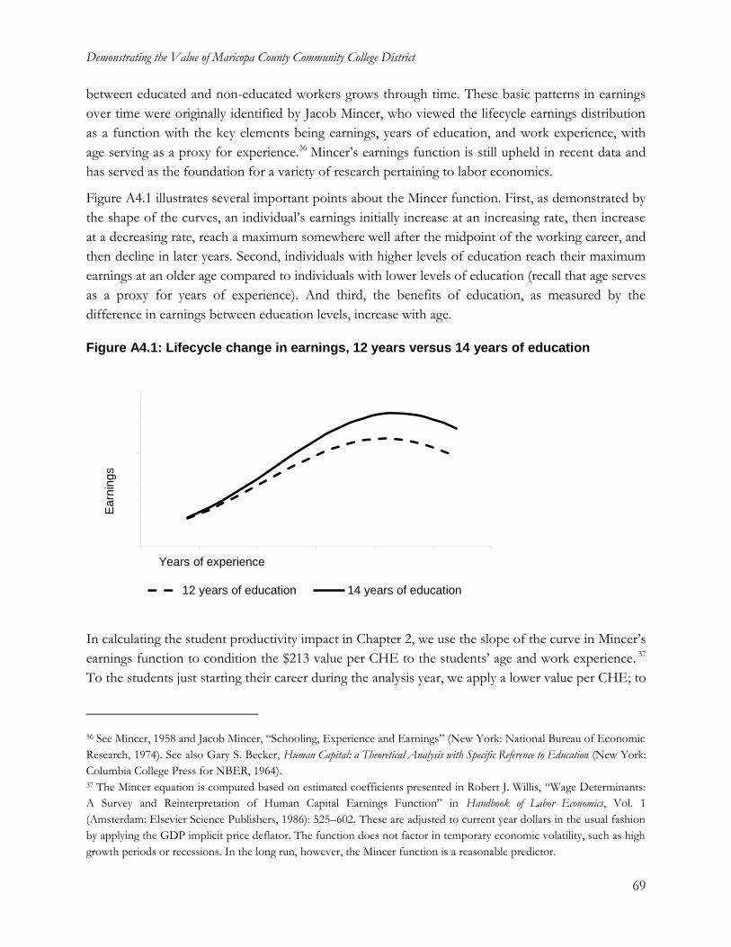
Demonstrating the Value of Maricopa County Community College District
69
between educated and non-educated workers grows through time. These basic patterns in earnings
over time were originally identified by Jacob Mincer, who viewed the lifecycle earnings distribution
as a function with the key elements being earnings, years of education, and work experience, with
age serving as a proxy for experience.36 Mincer’s earnings function is still upheld in recent data and
has served as the foundation for a variety of research pertaining to labor economics.
Figure A4.1 illustrates several important points about the Mincer function. First, as demonstrated by
the shape of the curves, an individual’s earnings initially increase at an increasing rate, then increase
at a decreasing rate, reach a maximum somewhere well after the midpoint of the working career, and
then decline in later years. Second, individuals with higher levels of education reach their maximum
earnings at an older age compared to individuals with lower levels of education (recall that age serves
as a proxy for years of experience). And third, the benefits of education, as measured by the
difference in earnings between education levels, increase with age.
Figure A4.1: Lifecycle change in earnings, 12 years versus 14 years of education
In calculating the student productivity impact in Chapter 2, we use the slope of the curve in Mincer’s
earnings function to condition the $213 value per CHE to the students’ age and work experience. 37
To the students just starting their career during the analysis year, we apply a lower value per CHE; to
36 See Mincer, 1958 and Jacob Mincer, “Schooling, Experience and Earnings” (New York: National Bureau of Economic
Research, 1974). See also Gary S. Becker, Human Capital: a Theoretical Analysis with Specific Reference to Education (New York:
Columbia College Press for NBER, 1964). 37 The Mincer equation is computed based on estimated coefficients presented in Robert J. Willis, “Wage Determinants:
A Survey and Reinterpretation of Human Capital Earnings Function” in Handbook of Labor Economics, Vol. 1
(Amsterdam: Elsevier Science Publishers, 1986): 525–602. These are adjusted to current year dollars in the usual fashion
by applying the GDP implicit price deflator. The function does not factor in temporary economic volatility, such as high
growth periods or recessions. In the long run, however, the Mincer function is a reasonable predictor.
Earn
ings
Years of experience
12 years of education 14 years of education
Demonstrating the Value of Maricopa County Community College District
70
the students in the latter half or approaching the end of their careers we apply a higher value per
CHE. The original $213 value per CHE applies only to the CHE production of students precisely at
the midpoint of their careers during the analysis year.
In Chapter 3 we again apply the Mincer function, this time to project the benefits stream of
MCCCD’s 2013-14 student population into the future. Here too the value per CHE is lower for
students at the start of their career and higher near the end of it, in accordance with the scalars
derived from the slope of the Mincer curve illustrated in Figure A4.1.
A4.3 Conclusion
This appendix demonstrates the significance of the value per CHE and the Mincer function in
determining the initial effect of student productivity on the regional economy in Chapter 2 and the
students’ return on their educational investment in Chapter 3. Both chapters provide further
discussion on the role that the students’ CHE production and corresponding increase in earnings
play in calculating the study outcomes.
Demonstrating the Value of Maricopa County Community College District
71
Appendix 5: Alternative Education Variable
In a scenario where MCCCD did not exist, some of its students would still be able to avail
themselves of an alternative comparable education. These students create benefits in the state even
in the absence of the institutions. The alternative education variable accounts for these students and
is used to discount the benefits we attribute to MCCCD.
Recall this analysis considers only relevent economic information regarding Maricopa County
Community College District. Considering the existence of various other academic institutions
surrounding MCCCD, we have to assume that a portion of students would find alternative
educations and either remain in or return to Arizona. For example, some students may participate in
online programs hosted at non-MCCCD institutions while remaining in Arizona. Others may attend
an out-of-state institution and return to Arizona upon completing their studies. For these students –
who would have found an alternative education and produced benefits in Arizona regardless of the
presence of MCCCD – we discount the benefits attributed to MCCCD. An important distinction
must be made here: the benefits from students who would find alternative educations outside the
county and not return to Arizona are not discounted. Because these benefits would not occur in
Arizona without the presence of MCCCD, they must be included.
In the absence of MCCCD, we assume 20% of MCCCD students would find alternative education
opportunities and remain in or return to Arizona. We account for this by discounting the alumni
impact, the benefits to taxpayers, and the benefits to society as a whole in sections 3 and 4 by 20%.
In other words, we assume 20% of the benefits created by MCCCD students would have occurred
anyways in the counterfactual scenario where MCCCD did not exist. A sensitivity analysis of this
adjustment is presented in section 5.
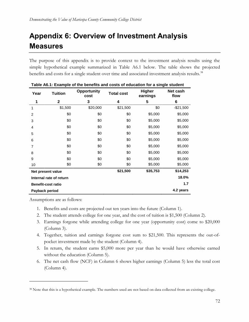
Demonstrating the Value of Maricopa County Community College District
72
Appendix 6: Overview of Investment Analysis
Measures
The purpose of this appendix is to provide context to the investment analysis results using the
simple hypothetical example summarized in Table A6.1 below. The table shows the projected
benefits and costs for a single student over time and associated investment analysis results.38
Table A6.1: Example of the benefits and costs of education for a single student
Year Tuition Opportunity
cost Total cost
Higher earnings
Net cash flow
1 2 3 4 5 6
1 $1,500 $20,000 $21,500 $0 -$21,500
2 $0 $0 $0 $5,000 $5,000
3 $0 $0 $0 $5,000 $5,000
4 $0 $0 $0 $5,000 $5,000
5 $0 $0 $0 $5,000 $5,000
6 $0 $0 $0 $5,000 $5,000
7 $0 $0 $0 $5,000 $5,000
8 $0 $0 $0 $5,000 $5,000
9 $0 $0 $0 $5,000 $5,000
10 $0 $0 $0 $5,000 $5,000
Net present value $21,500 $35,753 $14,253
Internal rate of return 18.0%
Benefit-cost ratio 1.7
Payback period 4.2 years
Assumptions are as follows:
1. Benefits and costs are projected out ten years into the future (Column 1).
2. The student attends college for one year, and the cost of tuition is $1,500 (Column 2).
3. Earnings forgone while attending college for one year (opportunity cost) come to $20,000
(Column 3).
4. Together, tuition and earnings forgone cost sum to $21,500. This represents the out-of-
pocket investment made by the student (Column 4).
5. In return, the student earns $5,000 more per year than he would have otherwise earned
without the education (Column 5).
6. The net cash flow (NCF) in Column 6 shows higher earnings (Column 5) less the total cost
(Column 4).
38 Note that this is a hypothetical example. The numbers used are not based on data collected from an existing college.

Demonstrating the Value of Maricopa County Community College District
73
7. The assumed “going rate” of interest is 4%, the rate of return from alternative investment
schemes for the use of the $21,500.
Results are expressed in standard investment analysis terms, which are as follows: the net present
value, the internal rate of return, the benefit-cost ratio, and the payback period. Each of these is
briefly explained below in the context of the cash flow numbers presented in Table A6.1.
A6.1 Net present value
The student in Table A6.1 can choose either to attend college or to forgo post-secondary education
and maintain his present employment. If he decides to enroll, certain economic implications unfold.
Tuition and fees must be paid, and earnings will cease for one year. In exchange, the student
calculates that with post-secondary education, his income will increase by at least the $5,000 per
year, as indicated in the table.
The question is simple – will the prospective student be economically better off by choosing to
enroll? If he adds up higher earnings of $5,000 per year for the remaining nine years in Table 1, the
total will be $45,000. Compared to a total investment of $21,500, this appears to be a very solid
investment. The reality, however, is different. Benefits are far lower than $45,000 because future
money is worth less than present money. Costs (tuition plus earnings forgone) are felt immediately
because they are incurred today, in the present. Benefits, on the other hand, occur in the future.
They are not yet available. All future benefits must be discounted by the going rate of interest
(referred to as the discount rate) to be able to express them in present value terms.39
Let us take a brief example. At 4%, the present value of $5,000 to be received one year from today is
$4,807. If the $5,000 were to be received in year ten, the present value would reduce to $3,377. Put
another way, $4,807 deposited in the bank today earning 4% interest will grow to $5,000 in one year;
and $3,377 deposited today would grow to $5,000 in ten years. An “economically rational” person
would, therefore, be equally satisfied receiving $3,377 today or $5,000 ten years from today given the
going rate of interest of 4%. The process of discounting – finding the present value of future higher
earnings – allows the model to express values on an equal basis in future or present value terms.
The goal is to express all future higher earnings in present value terms so that they can be compared
to investments incurred today (in this example, tuition plus earnings forgone). As indicated in Table
A6.1, the cumulative present value of $5,000 worth of higher earnings between years 2 and 10 is
$35,753 given the 4% interest rate, far lower than the undiscounted $45,000 discussed above.
The net present value of the investment is $14,253. This is simply the present value of the benefits
less the present value of the costs, or $35,753 - $21,500 = $14,253. In other words, the present value
39 Technically, the interest rate is applied to compounding – the process of looking at deposits today and determining
how much they will be worth in the future. The same interest rate is called a discount rate when the process is reversed –
determining the present value of future earnings.
Demonstrating the Value of Maricopa County Community College District
74
of benefits exceeds the present value of costs by as much as $14,253. The criterion for an
economically worthwhile investment is that the net present value is equal to or greater than zero.
Given this result, it can be concluded that, in this case, and given these assumptions, this particular
investment in education is very strong.
A6.2 Internal rate of return
The internal rate of return is another way of measuring the worth of investing in education using the
same cash flows shown in Table A6.1. In technical terms, the internal rate of return is a measure of
the average earning power of money used over the life of the investment. It is simply the interest
rate that makes the net present value equal to zero. In the discussion of the net present value above,
the model applies the “going rate” of interest of 4% and computes a positive net present value of
$14,253. The question now is what the interest rate would have to be in order to reduce the net
present value to zero. Obviously it would have to be higher – 18.0% in fact, as indicated in Table
A6.1. Or, if a discount rate of 18.0% were applied to the net present value calculations instead of the
4%, then the net present value would reduce to zero.
What does this mean? The internal rate of return of 18.0% defines a breakeven solution – the point
where the present value of benefits just equals the present value of costs, or where the net present
value equals zero. Or, at 18.0%, higher incomes of $5,000 per year for the next nine years will earn
back all investments of $21,500 made plus pay 18.0% for the use of that money ($21,500) in the
meantime. Is this a good return? Indeed it is. If it is compared to the 4% “going rate” of interest
applied to the net present value calculations, 18.0% is far higher than 4%. It may be concluded,
therefore, that the investment in this case is solid. Alternatively, comparing the 18.0% rate of return
to the long-term 7% rate or so obtained from investments in stocks and bonds also indicates that
the investment in education is strong relative to the stock market returns (on average).
A word of caution – the approach for calculating the internal rate of return can sometimes generate
wild or unbelievable results that defy the imagination. Technically, the approach requires at least one
negative cash flow to offset all subsequent positive flows. For example, if the student works full-
time while attending college, the opportunity cost of time would be much lower. The only out-of-
pocket cost would be the $1,500 paid for tuition. In this case, it would still be possible to compute
the internal rate of return, but it would be a staggering 333% because only a negative $1,500 cash
flow would be offsetting nine subsequent years of $5,000 worth of higher earnings. Although the
333% return would technically be correct, it would not be consistent with the conventional
understanding of returns expressed as percentages.
A6.3 Benefit-cost ratio
The benefit-cost ratio is simply the present value of benefits divided by present value of costs, or
$35,753 ÷ $21,500 = 1.7 (based on the 4% discount rate). Of course, any change in the discount rate
would also change the benefit-cost ratio. Applying the 18.0% internal rate of return discussed above
Demonstrating the Value of Maricopa County Community College District
75
would reduce the benefit-cost ratio to 1.0, the breakeven solution where benefits just equal costs.
Applying a discount rate higher than the 18.0% would reduce the ratio to lower than 1.0, and the
investment would not be feasible. The 1.7 ratio means that a dollar invested today will return a
cumulative $1.70 over the ten-year time period.
A6.4 Payback period
This is the length of time from the beginning of the investment (consisting of tuition and earnings
forgone) until higher future earnings give a return on the investment made. For the student in Table
A6.1, it will take roughly 4.2 years of $5,000 worth of higher earnings to recapture his investment of
$1,500 in tuition and the $20,000 in earnings forgone while attending college. Higher earnings that
occur beyond 4.2 years are the returns that make the investment in education in this example
economically worthwhile. The payback period is a fairly rough, albeit common, means of choosing
between investments. The shorter the payback period, the stronger the investment.
Demonstrating the Value of Maricopa County Community College District
76
Appendix 7: Shutdown Point
The investment analysis in Chapter 3 weighs the benefits generated by the district against the state
and local taxpayer funding that the district receives to support its operations. An important part of
this analysis is factoring out the benefits that the district would have been able to generate anyway,
even without state and local taxpayer support. This adjustment is used to establish a direct link
between what taxpayers pay and what they receive in return. If the district is able to generate
benefits without taxpayer support, then it would not be a true investment.40
The overall approach includes a sub-model that simulates the effect on student enrollment if the
district loses its state and local funding and has to raise student tuition and fees in order to stay
open. If the district can still operate without state and local support, then any benefits it generates at
that level are discounted from total benefit estimates. If the simulation indicates that the district
cannot stay open, however, then benefits are directly linked to costs, and no discounting applies.
This appendix documents the underlying theory behind these adjustments.
A7.1 State and local government support versus student demand for
education
Figure A7.1 presents a simple model of student demand and state and local government support.
The right side of the graph is a standard demand curve (D) showing student enrollment as a function
of student tuition and fees. Enrollment is measured in terms of total credit hour equivalents (CHEs)
and expressed as a percentage of the district’s current CHE production. Current student tuition and
fees are represented by p', and state and local government support covers C% of all costs. At this
point in the analysis, it is assumed that the district has only two sources of revenues: 1) student
tuition and fees and 2) state and local government support.
40 Of course, as a public training provider, MCCCD would not be permitted to continue without public funding, so the
situation in which it would lose all state support is entirely hypothetical. The purpose of the adjustment factor is to
examine MCCCD in standard investment analysis terms by netting out any benefits it may be able to generate that are
not directly linked to the costs of supporting it.
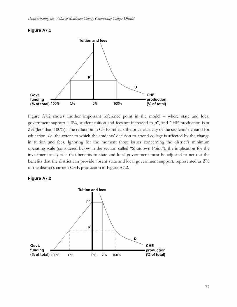
Demonstrating the Value of Maricopa County Community College District
77
Figure A7.1
Figure A7.2 shows another important reference point in the model – where state and local
government support is 0%, student tuition and fees are increased to p'', and CHE production is at
Z% (less than 100%). The reduction in CHEs reflects the price elasticity of the students’ demand for
education, i.e., the extent to which the students’ decision to attend college is affected by the change
in tuition and fees. Ignoring for the moment those issues concerning the district’s minimum
operating scale (considered below in the section called “Shutdown Point”), the implication for the
investment analysis is that benefits to state and local government must be adjusted to net out the
benefits that the district can provide absent state and local government support, represented as Z%
of the district’s current CHE production in Figure A7.2.
Figure A7.2
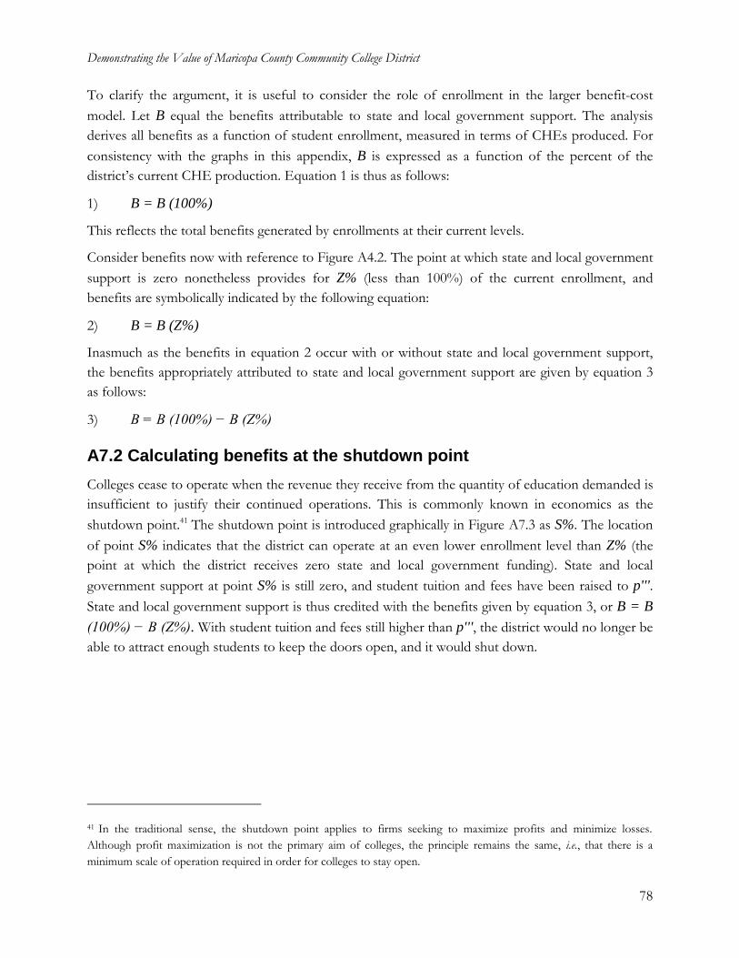
Demonstrating the Value of Maricopa County Community College District
78
To clarify the argument, it is useful to consider the role of enrollment in the larger benefit-cost
model. Let B equal the benefits attributable to state and local government support. The analysis
derives all benefits as a function of student enrollment, measured in terms of CHEs produced. For
consistency with the graphs in this appendix, B is expressed as a function of the percent of the
district’s current CHE production. Equation 1 is thus as follows:
1) B = B (100%)
This reflects the total benefits generated by enrollments at their current levels.
Consider benefits now with reference to Figure A4.2. The point at which state and local government
support is zero nonetheless provides for Z% (less than 100%) of the current enrollment, and
benefits are symbolically indicated by the following equation:
2) B = B (Z%)
Inasmuch as the benefits in equation 2 occur with or without state and local government support,
the benefits appropriately attributed to state and local government support are given by equation 3
as follows:
3) B = B (100%) − B (Z%)
A7.2 Calculating benefits at the shutdown point
Colleges cease to operate when the revenue they receive from the quantity of education demanded is
insufficient to justify their continued operations. This is commonly known in economics as the
shutdown point.41 The shutdown point is introduced graphically in Figure A7.3 as S%. The location
of point S% indicates that the district can operate at an even lower enrollment level than Z% (the
point at which the district receives zero state and local government funding). State and local
government support at point S% is still zero, and student tuition and fees have been raised to p'''.
State and local government support is thus credited with the benefits given by equation 3, or B = B
(100%) − B (Z%). With student tuition and fees still higher than p''', the district would no longer be
able to attract enough students to keep the doors open, and it would shut down.
41 In the traditional sense, the shutdown point applies to firms seeking to maximize profits and minimize losses.
Although profit maximization is not the primary aim of colleges, the principle remains the same, i.e., that there is a
minimum scale of operation required in order for colleges to stay open.
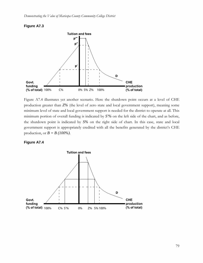
Demonstrating the Value of Maricopa County Community College District
79
Figure A7.3
Figure A7.4 illustrates yet another scenario. Here the shutdown point occurs at a level of CHE
production greater than Z% (the level of zero state and local government support), meaning some
minimum level of state and local government support is needed for the district to operate at all. This
minimum portion of overall funding is indicated by S'% on the left side of the chart, and as before,
the shutdown point is indicated by S% on the right side of chart. In this case, state and local
government support is appropriately credited with all the benefits generated by the district’s CHE
production, or B = B (100%).
Figure A7.4
Demonstrating the Value of Maricopa County Community College District
80
Appendix 8: Social Externalities
Education has a predictable and positive effect on a diverse array of social benefits. These, when
quantified in dollar terms, represent significant social savings that directly benefit society as a whole,
including taxpayers. In this appendix we discuss the following three main benefit categories: 1)
improved health, 2) reductions in crime, and 3) reductions in welfare and unemployment.
It is important to note that the data and estimates presented here should not be viewed as exact, but
rather as indicative of the positive impacts of education on an individual’s quality of life. The process
of quantifying these impacts requires a number of assumptions to be made, creating a level of
uncertainty that should be borne in mind when reviewing the results.
A8.1 Health
Statistics clearly show the correlation between increases in education and improved health. The
manifestations of this are found in five health-related variables: smoking, alcoholism, obesity, mental
illness, and drug abuse. There are other health-related areas that link to educational attainment, but
these are omitted from the analysis until we can invoke adequate (and mutually exclusive) databases
and are able to fully develop the functional relationships between them.
A8.1.1 Smoking
Despite a marked decline over the last several decades in the percentage of U.S. residents that
smoke, a sizeable percentage of the U.S. population still uses tobacco. The negative health effects of
smoking are well documented in the literature, which identifies smoking as one of the most serious
health issues in the U.S.
Figure A8.1 shows the prevalence of cigarette smoking among adults aged 25 years and over, based
on data provided by the National Health Interview Survey.42 As indicated, the percent of persons
who smoke begins to decline beyond the level of high school education.
42 Centers for Disease Control and Prevention, “Table 61. Age-adjusted prevalence of current cigarette smoking among
adults aged 25 and over, by sex, race, and education level: United States, selected years 1974-2011,” National Health
Interview Survey, 2011.
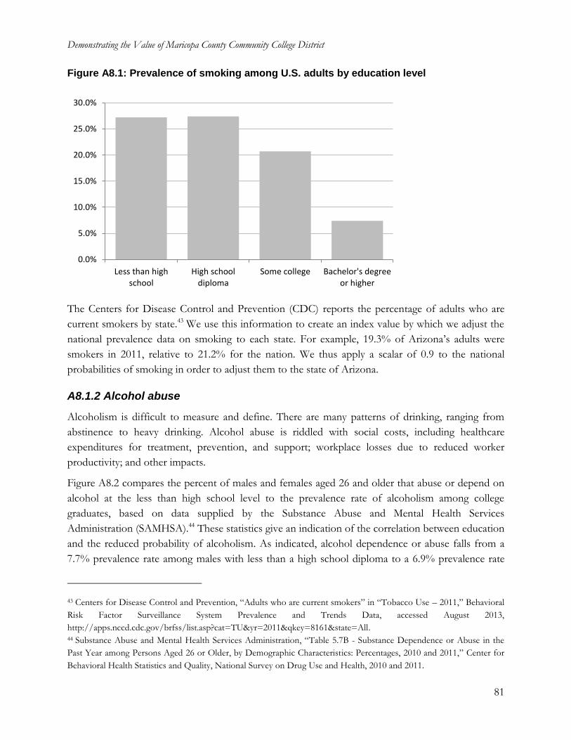
Demonstrating the Value of Maricopa County Community College District
81
Figure A8.1: Prevalence of smoking among U.S. adults by education level
The Centers for Disease Control and Prevention (CDC) reports the percentage of adults who are
current smokers by state.43 We use this information to create an index value by which we adjust the
national prevalence data on smoking to each state. For example, 19.3% of Arizona’s adults were
smokers in 2011, relative to 21.2% for the nation. We thus apply a scalar of 0.9 to the national
probabilities of smoking in order to adjust them to the state of Arizona.
A8.1.2 Alcohol abuse
Alcoholism is difficult to measure and define. There are many patterns of drinking, ranging from
abstinence to heavy drinking. Alcohol abuse is riddled with social costs, including healthcare
expenditures for treatment, prevention, and support; workplace losses due to reduced worker
productivity; and other impacts.
Figure A8.2 compares the percent of males and females aged 26 and older that abuse or depend on
alcohol at the less than high school level to the prevalence rate of alcoholism among college
graduates, based on data supplied by the Substance Abuse and Mental Health Services
Administration (SAMHSA).44 These statistics give an indication of the correlation between education
and the reduced probability of alcoholism. As indicated, alcohol dependence or abuse falls from a
7.7% prevalence rate among males with less than a high school diploma to a 6.9% prevalence rate
43 Centers for Disease Control and Prevention, “Adults who are current smokers” in “Tobacco Use – 2011,” Behavioral
Risk Factor Surveillance System Prevalence and Trends Data, accessed August 2013,
http://apps.nccd.cdc.gov/brfss/list.asp?cat=TU&yr=2011&qkey=8161&state=All. 44 Substance Abuse and Mental Health Services Administration, “Table 5.7B - Substance Dependence or Abuse in the
Past Year among Persons Aged 26 or Older, by Demographic Characteristics: Percentages, 2010 and 2011,” Center for
Behavioral Health Statistics and Quality, National Survey on Drug Use and Health, 2010 and 2011.
0.0%
5.0%
10.0%
15.0%
20.0%
25.0%
30.0%
Less than highschool
High schooldiploma
Some college Bachelor's degreeor higher
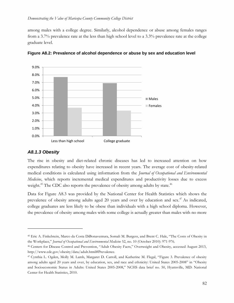
Demonstrating the Value of Maricopa County Community College District
82
among males with a college degree. Similarly, alcohol dependence or abuse among females ranges
from a 3.7% prevalence rate at the less than high school level to a 3.3% prevalence rate at the college
graduate level.
Figure A8.2: Prevalence of alcohol dependence or abuse by sex and education level
A8.1.3 Obesity
The rise in obesity and diet-related chronic diseases has led to increased attention on how
expenditures relating to obesity have increased in recent years. The average cost of obesity-related
medical conditions is calculated using information from the Journal of Occupational and Environmental
Medicine, which reports incremental medical expenditures and productivity losses due to excess
weight.45 The CDC also reports the prevalence of obesity among adults by state.46
Data for Figure A8.3 was provided by the National Center for Health Statistics which shows the
prevalence of obesity among adults aged 20 years and over by education and sex.47 As indicated,
college graduates are less likely to be obese than individuals with a high school diploma. However,
the prevalence of obesity among males with some college is actually greater than males with no more
45 Eric A. Finkelstein, Marco da Costa DiBonaventura, Somali M. Burgess, and Brent C. Hale, “The Costs of Obesity in
the Workplace,” Journal of Occupational and Environmental Medicine 52, no. 10 (October 2010): 971-976. 46 Centers for Disease Control and Prevention, “Adult Obesity Facts,” Overweight and Obesity, accessed August 2013,
http://www.cdc.gov/obesity/data/adult.html#Prevalence. 47 Cynthia L. Ogden, Molly M. Lamb, Margaret D. Carroll, and Katherine M. Flegal, “Figure 3. Prevalence of obesity
among adults aged 20 years and over, by education, sex, and race and ethnicity: United States 2005-2008” in “Obesity
and Socioeconomic Status in Adults: United States 2005-2008,” NCHS data brief no. 50, Hyattsville, MD: National
Center for Health Statistics, 2010.
0.0%
1.0%
2.0%
3.0%
4.0%
5.0%
6.0%
7.0%
8.0%
9.0%
Less than high school College graduate
Males
Females
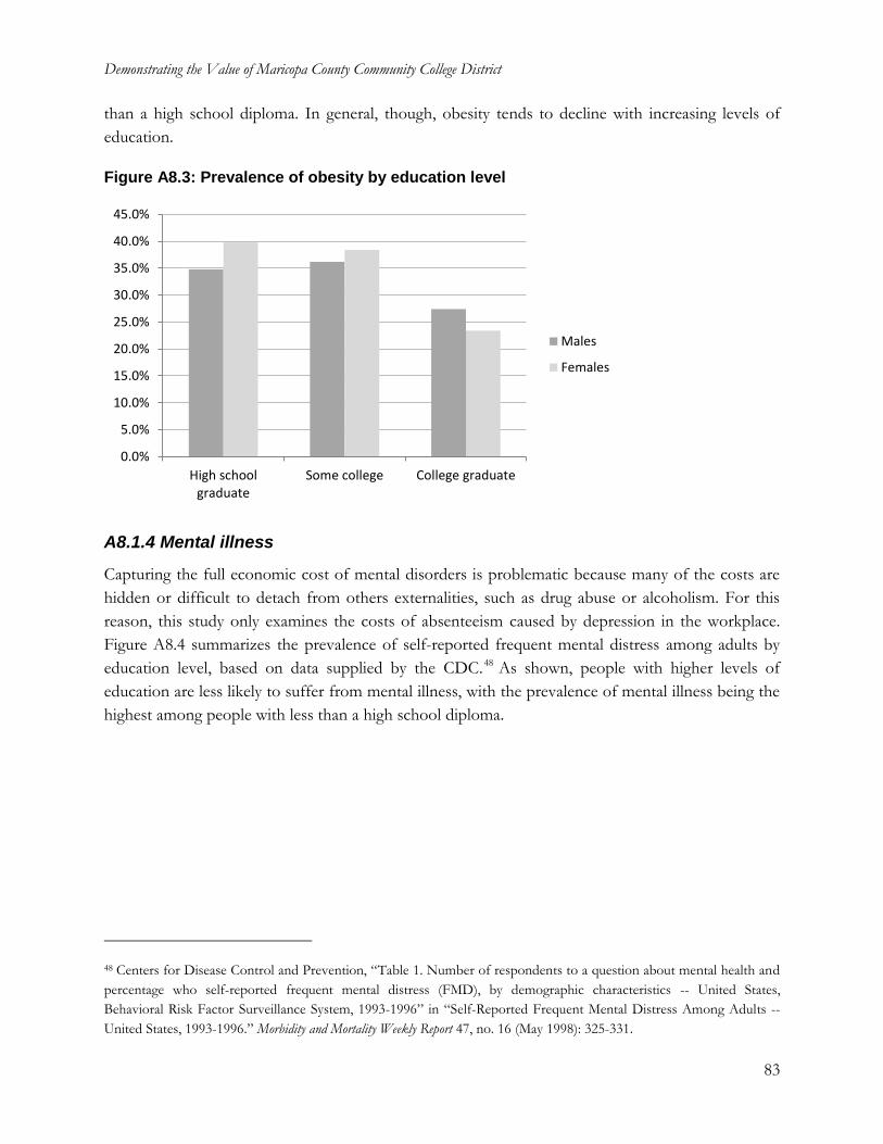
Demonstrating the Value of Maricopa County Community College District
83
than a high school diploma. In general, though, obesity tends to decline with increasing levels of
education.
Figure A8.3: Prevalence of obesity by education level
A8.1.4 Mental illness
Capturing the full economic cost of mental disorders is problematic because many of the costs are
hidden or difficult to detach from others externalities, such as drug abuse or alcoholism. For this
reason, this study only examines the costs of absenteeism caused by depression in the workplace.
Figure A8.4 summarizes the prevalence of self-reported frequent mental distress among adults by
education level, based on data supplied by the CDC.48 As shown, people with higher levels of
education are less likely to suffer from mental illness, with the prevalence of mental illness being the
highest among people with less than a high school diploma.
48 Centers for Disease Control and Prevention, “Table 1. Number of respondents to a question about mental health and
percentage who self-reported frequent mental distress (FMD), by demographic characteristics -- United States,
Behavioral Risk Factor Surveillance System, 1993-1996” in “Self-Reported Frequent Mental Distress Among Adults --
United States, 1993-1996.” Morbidity and Mortality Weekly Report 47, no. 16 (May 1998): 325-331.
0.0%
5.0%
10.0%
15.0%
20.0%
25.0%
30.0%
35.0%
40.0%
45.0%
High schoolgraduate
Some college College graduate
Males
Females
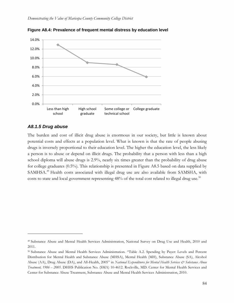
Demonstrating the Value of Maricopa County Community College District
84
Figure A8.4: Prevalence of frequent mental distress by education level
A8.1.5 Drug abuse
The burden and cost of illicit drug abuse is enormous in our society, but little is known about
potential costs and effects at a population level. What is known is that the rate of people abusing
drugs is inversely proportional to their education level. The higher the education level, the less likely
a person is to abuse or depend on illicit drugs. The probability that a person with less than a high
school diploma will abuse drugs is 2.9%, nearly six times greater than the probability of drug abuse
for college graduates (0.5%). This relationship is presented in Figure A8.5 based on data supplied by
SAMHSA.49 Health costs associated with illegal drug use are also available from SAMSHA, with
costs to state and local government representing 48% of the total cost related to illegal drug use.50
49 Substance Abuse and Mental Health Services Administration, National Survey on Drug Use and Health, 2010 and
2011. 50 Substance Abuse and Mental Health Services Administration. “Table A.2. Spending by Payer: Levels and Percent
Distribution for Mental Health and Substance Abuse (MHSA), Mental Health (MH), Substance Abuse (SA), Alcohol
Abuse (AA), Drug Abuse (DA), and All-Health, 2005” in National Expenditures for Mental Health Services & Substance Abuse
Treatment, 1986 – 2005. DHHS Publication No. (SMA) 10-4612. Rockville, MD: Center for Mental Health Services and
Center for Substance Abuse Treatment, Substance Abuse and Mental Health Services Administration, 2010.
0.0%
2.0%
4.0%
6.0%
8.0%
10.0%
12.0%
14.0%
Less than highschool
High schoolgraduate
Some college ortechnical school
College graduate
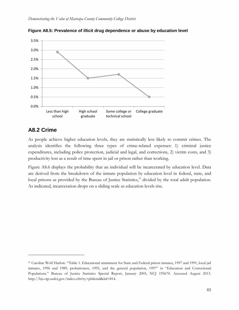
Demonstrating the Value of Maricopa County Community College District
85
Figure A8.5: Prevalence of illicit drug dependence or abuse by education level
A8.2 Crime
As people achieve higher education levels, they are statistically less likely to commit crimes. The
analysis identifies the following three types of crime-related expenses: 1) criminal justice
expenditures, including police protection, judicial and legal, and corrections, 2) victim costs, and 3)
productivity lost as a result of time spent in jail or prison rather than working.
Figure A8.6 displays the probability that an individual will be incarcerated by education level. Data
are derived from the breakdown of the inmate population by education level in federal, state, and
local prisons as provided by the Bureau of Justice Statistics,51 divided by the total adult population.
As indicated, incarceration drops on a sliding scale as education levels rise.
51 Caroline Wolf Harlow. “Table 1. Educational attainment for State and Federal prison inmates, 1997 and 1991, local jail
inmates, 1996 and 1989, probationers, 1995, and the general population, 1997” in “Education and Correctional
Populations.” Bureau of Justice Statistics Special Report, January 2003, NCJ 195670. Accessed August 2013.
http://bjs.ojp.usdoj.gov/index.cfm?ty=pbdetail&iid=814.
0.0%
0.5%
1.0%
1.5%
2.0%
2.5%
3.0%
3.5%
Less than highschool
High schoolgraduate
Some college ortechnical school
College graduate
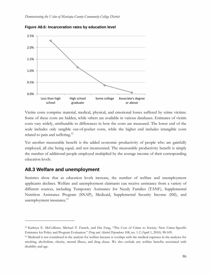
Demonstrating the Value of Maricopa County Community College District
86
Figure A8.6: Incarceration rates by education level
Victim costs comprise material, medical, physical, and emotional losses suffered by crime victims.
Some of these costs are hidden, while others are available in various databases. Estimates of victim
costs vary widely, attributable to differences in how the costs are measured. The lower end of the
scale includes only tangible out-of-pocket costs, while the higher end includes intangible costs
related to pain and suffering.52
Yet another measurable benefit is the added economic productivity of people who are gainfully
employed, all else being equal, and not incarcerated. The measurable productivity benefit is simply
the number of additional people employed multiplied by the average income of their corresponding
education levels.
A8.3 Welfare and unemployment
Statistics show that as education levels increase, the number of welfare and unemployment
applicants declines. Welfare and unemployment claimants can receive assistance from a variety of
different sources, including Temporary Assistance for Needy Families (TANF), Supplemental
Nutrition Assistance Program (SNAP), Medicaid, Supplemental Security Income (SSI), and
unemployment insurance.53
52 Kathryn E. McCollister, Michael T. French, and Hai Fang, “The Cost of Crime to Society: New Crime-Specific
Estimates for Policy and Program Evaluation.” Drug and Alcohol Dependence 108, no. 1-2 (April 1, 2010): 98-109. 53 Medicaid is not considered in the analysis for welfare because it overlaps with the medical expenses in the analyses for
smoking, alcoholism, obesity, mental illness, and drug abuse. We also exclude any welfare benefits associated with
disability and age.
0.0%
0.5%
1.0%
1.5%
2.0%
2.5%
Less than highschool
High schoolgraduate
Some college Associate's degreeor above
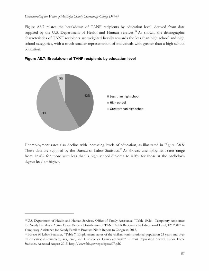
Demonstrating the Value of Maricopa County Community College District
87
Figure A8.7 relates the breakdown of TANF recipients by education level, derived from data
supplied by the U.S. Department of Health and Human Services.54 As shown, the demographic
characteristics of TANF recipients are weighted heavily towards the less than high school and high
school categories, with a much smaller representation of individuals with greater than a high school
education.
Figure A8.7: Breakdown of TANF recipients by education level
Unemployment rates also decline with increasing levels of education, as illustrated in Figure A8.8.
These data are supplied by the Bureau of Labor Statistics.55 As shown, unemployment rates range
from 12.4% for those with less than a high school diploma to 4.0% for those at the bachelor’s
degree level or higher.
54 U.S. Department of Health and Human Services, Office of Family Assistance, “Table 10:26 - Temporary Assistance
for Needy Families - Active Cases: Percent Distribution of TANF Adult Recipients by Educational Level, FY 2009” in
Temporary Assistance for Needy Families Program Ninth Report to Congress, 2012. 55 Bureau of Labor Statistics, “Table 7. Employment status of the civilian noninstitutional population 25 years and over
by educational attainment, sex, race, and Hispanic or Latino ethnicity.” Current Population Survey, Labor Force
Statistics. Accessed August 2013. http://www.bls.gov/cps/cpsaat07.pdf.
42%
53%
5%
Less than high school
High school
Greater than high school
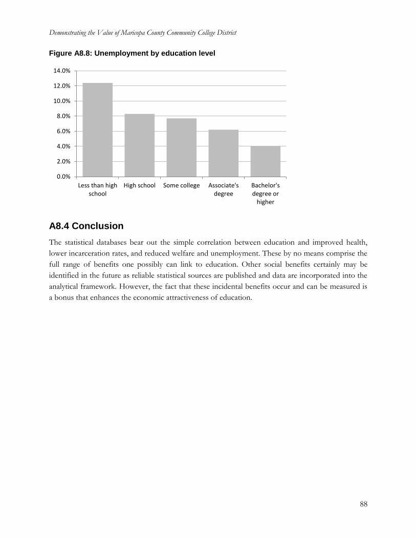
Demonstrating the Value of Maricopa County Community College District
88
Figure A8.8: Unemployment by education level
A8.4 Conclusion
The statistical databases bear out the simple correlation between education and improved health,
lower incarceration rates, and reduced welfare and unemployment. These by no means comprise the
full range of benefits one possibly can link to education. Other social benefits certainly may be
identified in the future as reliable statistical sources are published and data are incorporated into the
analytical framework. However, the fact that these incidental benefits occur and can be measured is
a bonus that enhances the economic attractiveness of education.
0.0%
2.0%
4.0%
6.0%
8.0%
10.0%
12.0%
14.0%
Less than highschool
High school Some college Associate'sdegree
Bachelor'sdegree or
higher