© Wing Kam Liu, Eduard G. Karpov,Harold Park, David Farrell, Dept. of Mechanical Engineering, Northwestern University 1

Demonstrate Teaching FEM, Particle Dynamics, and Simple MD Codes Using Matlab & Mathematica

© Wing Kam Liu, Eduard G. Karpov,Harold Park, David Farrell, Dept. of Mechanical Engineering, Northwestern University 2

Recall from Lecture: the Lagrangian Method

1. The choice of s generalized coordinates (s – number of degrees of freedom).

2. Derivation of the kinetic and potential energy in terms of the generalized coordinates

3. The difference between the kinetic and potential energies gives the Lagrangian function.

4. Substitution of the Lagrange function into the Lagrangian equation of motion and derivation of a system of s second-order differential equations to be solved.

5. Solution of the equations of motion, using a numerical time-integration algorithm.

6. Post-processing and visualization.

Now, some examples

© Wing Kam Liu, Eduard G. Karpov,Harold Park, David Farrell, Dept. of Mechanical Engineering, Northwestern University 3

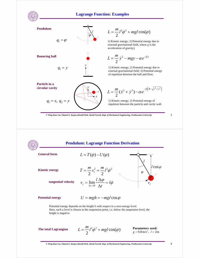
Lagrange Function: Examples

2 2 cos( )2

mL l mglϕ ϕ= +&

Pendulum

Bouncing ball

Particle in a circular cavity

2

2ym

L y mgy e βα −= − −&

y

( )2 22 2( )

2

R x ymL x y e

βα

− − += + −& &

1) Kinetic energy; 2) Potential energy due to external gravitational field, where g is the acceleration of gravity).

1) Kinetic energy; 2) Potential energy due to external gravitational field; 3) Potential energy of repulsion between the ball and floor.

1) Kinetic energy; 2) Potential energy of repulsion between the particle and cavity wall.

φl

y

x

1q ϕ=

1q y=

1 2,q x q y= =

© Wing Kam Liu, Eduard G. Karpov,Harold Park, David Farrell, Dept. of Mechanical Engineering, Northwestern University 4

Pendulum: Lagrange Function Derivation

( ) ( )L T Uϕ ϕ= −&General form

Kinetic energy

tangential velocity

Potential energy

The total Lagrangian

l

vτ

l cosφ2 2 2

2 2

m mT v lτ ϕ= = &

0lim

t

lv l

tτϕ ϕ

∆ →

∆= =

∆&

cosU mgh mgl ϕ= = −

Potential energy depends on the height h with respect to a zero-energy level. Here, such a level is chosen at the suspension point, i.e. below the suspension level, the height is negative.

2 2 cos( )2

mL l mglϕ ϕ= +& 29.8m/s , 2mg l= =

Parameters used:

φ

© Wing Kam Liu, Eduard G. Karpov,Harold Park, David Farrell, Dept. of Mechanical Engineering, Northwestern University 5

Pendulum: Equation of Motion and Solution

Lagrange function and equation motion:

Initial conditions (radian):

(0) 0.3, (0) 0ϕ ϕ= =&

( )2 2 cos 0 ( ) sin ( ) 02

m d L L gL l mgl t t

dt lϕ ϕ ϕ ϕ

ϕ ϕ∂ ∂

= + − = + =∂ ∂

⇒ ⇒& &&&

(0) 1.8, (0) 0ϕ ϕ= =& (0) 3.12, (0) 0ϕ ϕ= =&

29.8m/s , 2mg l= =Parameters:

© Wing Kam Liu, Eduard G. Karpov,Harold Park, David Farrell, Dept. of Mechanical Engineering, Northwestern University 6

Bouncing Ball: Lagrange Function Derivation

( ) ( )L T y U y= −&General form

Kinetic energy

Potential energy

2

2

mT y= &

yU mgy e βα −= +

Purple dashed line: the first term (gravitational interaction between the ball and the Earth).

Blue dotted line: the second term (repulsion between the ball and the bouncing surface).

Red solid line: the total potential.

β is a relative scaling factor: the ball-surface repulsive potential growths in eβ times for a unit length ball/surface penetration (from y = 0 to y = – 1m).

y

2( , )2

ymL y y y mgy e βα −= − −& &The total Lagrangian:

2

19.8m/s , 1kg,1J, 4m

g mα β −= == =

Parameters used:

© Wing Kam Liu, Eduard G. Karpov,Harold Park, David Farrell, Dept. of Mechanical Engineering, Northwestern University 7

Bouncing Ball: Equation of Motion and Solution

Lagrange function and equation motion:

Initial conditions:

(0) 5m(0) 0

yy

==&

2 ( )0 ( ) 02

y y tm d L LL y mgy e y t g e

dt y y mβ βαβα − −∂ ∂

= − − − = + − =∂

⇒ ⇒∂

& &&&

(0) 10m(0) 0

yy

==&

(0) 15m(0) 0

yy

==&

2 19.8m/s , 1kg, 1J, 4mg m α β −= = = =Parameters:

© Wing Kam Liu, Eduard G. Karpov,Harold Park, David Farrell, Dept. of Mechanical Engineering, Northwestern University 8

Particle in a Circular Cavity: Lagrange Function Derivation

( , ) ( , )L T x y U x y= −& &General form

Kinetic energy

Potential energy

The total Lagrangian

2 2( )2

mT x y= +& &

( ) ( )2 2R x yR rU e eββα α

− − +− −= =

The potential energy grows quickly and becomes larger than the typical kinetic energy, when the distance r between the particle and the center of the cavity approaches value R.

R is the effective radius of the cavity. At r < R, U does not alter the trajectory.

β is a relative scaling factor: the potential energy growths in eβ times between r = R and r = R+1.

( )2 22 2( , , , ) ( )

2

R x ymL x y x y x y e

βα

− − += + −& & & &

y

xr

R

© Wing Kam Liu, Eduard G. Karpov,Harold Park, David Farrell, Dept. of Mechanical Engineering, Northwestern University 9

Particle in a Circular Cavity: Equation of Motion and Solution

Lagrangian function and equations: Potential barrier:

(0) 2.522nm, (0) 0, (0) 0, (0) 30nm/sx x y y=− = = =& &

27 2 210 J, ( ) ( ) ( )r t x t y tα −= = +

1 94nm , 10nm, 10 kgR mβ − −= = =Parameters:

Initial conditions:

( )2 2 ( ( ))2 2

( ( ))

( ) ( )/ ( )( )

2 ( ) ( )/ ( )

R r tR x y

R r t

m x t e x t r tmL x y e

my t e y t r t

ββ

β

αβα

αβ

− −− − +

− −

⎧ = −= + −

−⇒ ⎨

=⎩

&&& &

&&

© Wing Kam Liu, Eduard G. Karpov,Harold Park, David Farrell, Dept. of Mechanical Engineering, Northwestern University 10

Recall from Lecture: Both Stable and Unstable Trajectories Possible

Stable quasiperiodic trajectory Unstable chaotic trajectory

© Wing Kam Liu, Eduard G. Karpov,Harold Park, David Farrell, Dept. of Mechanical Engineering, Northwestern University 11

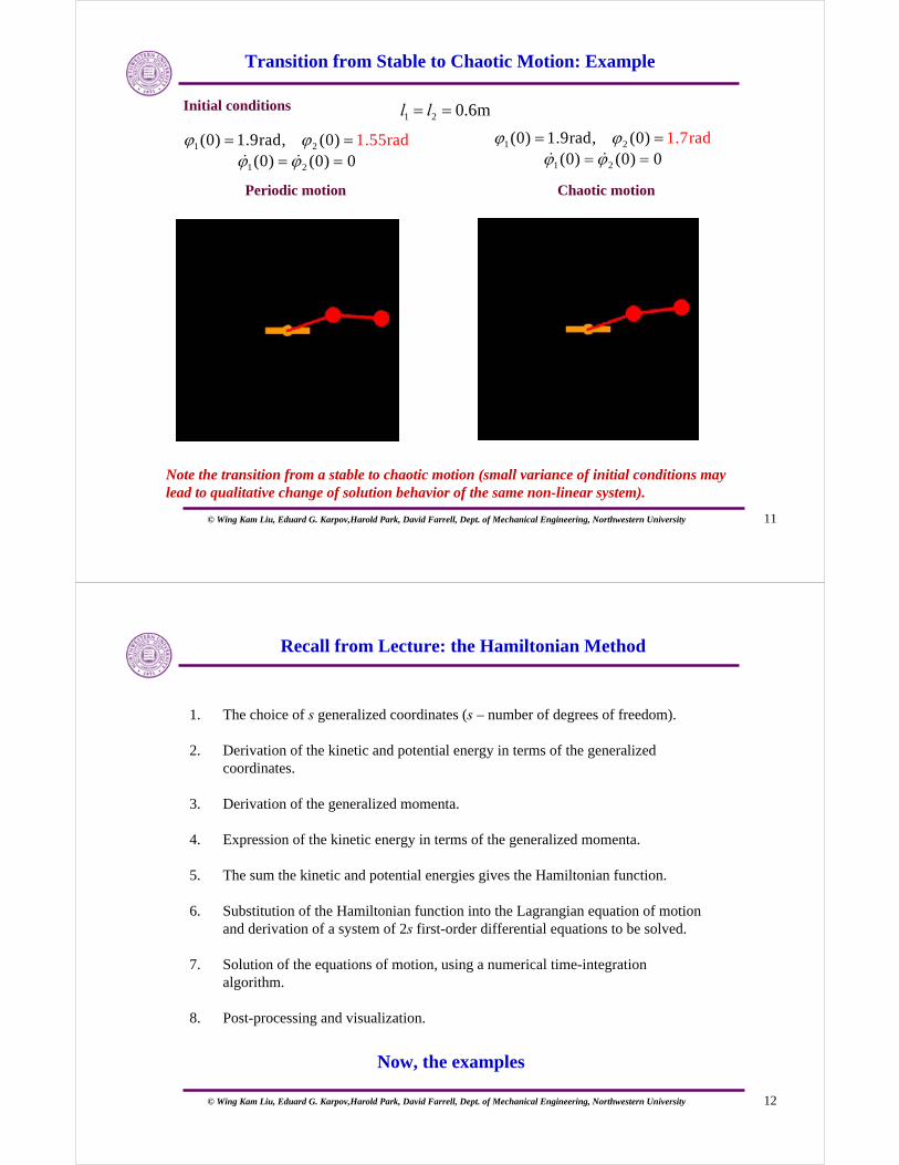
Transition from Stable to Chaotic Motion: Example

Initial conditions

1 2

1 2

1.55rad(0) 1.9rad, (0)(0) (0) 0

ϕ ϕϕ ϕ

= == =& &

1 2 0.6ml l= =

1 2

1 2

1.7rad(0) 1.9rad, (0)(0) (0) 0

ϕ ϕϕ ϕ= =

= =& &

Note the transition from a stable to chaotic motion (small variance of initial conditions may lead to qualitative change of solution behavior of the same non-linear system).

Periodic motion Chaotic motion

© Wing Kam Liu, Eduard G. Karpov,Harold Park, David Farrell, Dept. of Mechanical Engineering, Northwestern University 12

Recall from Lecture: the Hamiltonian Method

1. The choice of s generalized coordinates (s – number of degrees of freedom).

2. Derivation of the kinetic and potential energy in terms of the generalized coordinates.

3. Derivation of the generalized momenta.

4. Expression of the kinetic energy in terms of the generalized momenta.

5. The sum the kinetic and potential energies gives the Hamiltonian function.

6. Substitution of the Hamiltonian function into the Lagrangian equation of motion and derivation of a system of 2s first-order differential equations to be solved.

7. Solution of the equations of motion, using a numerical time-integration algorithm.

8. Post-processing and visualization.

Now, the examples

© Wing Kam Liu, Eduard G. Karpov,Harold Park, David Farrell, Dept. of Mechanical Engineering, Northwestern University 13

Hamiltonian Equations of Motion: Pendulum

Hamiltonian of the system:

2, , sin

H H pp p mgl

p mlϕ ϕ ϕ

ϕ∂ ∂

= = − = = −∂ ∂

⇒& && &

Equations of motion:

Lagrange function and the generalized momentum:

2 2 2cos2

m LL l mgl p mlϕ ϕ ϕ

ϕ∂

= + = =∂

⇒& &&

2 2

2 2, cos cos

2 2

p pT U mgl H mgl

ml mlϕ ϕ= −⇒= = −

2 sin sin 0g

p ml mgll

ϕ ϕ ϕ ϕ= = − =⇒ +&& &&&

Conversion to the Lagrangian form (elimination of p):

脨l

© Wing Kam Liu, Eduard G. Karpov,Harold Park, David Farrell, Dept. of Mechanical Engineering, Northwestern University 14

Hamiltonian Equations of Motion: Bouncing Ball

Hamiltonian of the system:

, , yH H py p y p mg e

p y mββ −⇒

∂ ∂= = − = = − +∂ ∂

& & & &

Equations of motion:

Lagrange function and the generalized momentum:

2

2ym L

L y mgy e p m yβ

ϕ− ∂

= − − = =∂

⇒& &&

2 2

,2 2

y yp pT U mgy e H mgy e

m mβ β− −= = + = + +⇒

0y yp my mg e y g em

β βββ − −⇒= = − + + − =& && &&

Conversion to the Lagrangian form (elimination of p):

y

© Wing Kam Liu, Eduard G. Karpov,Harold Park, David Farrell, Dept. of Mechanical Engineering, Northwestern University 15

Recall from Lecture: The Phase Space Trajectories: Examples

Examples of phase space trajectories:

(Projection to the plane x, px)

© Wing Kam Liu, Eduard G. Karpov,Harold Park, David Farrell, Dept. of Mechanical Engineering, Northwestern University 16

Recall from Lecture: the MD Simulation Procedure

• Model individual particles and boundaries.

• Model interaction between particles and between particles and boundaries.

• Assign initial positions and velocities.

• Solve the equations of motion.

• Simulate the movements of the system.

• Analyze the simulation data to investigate collective phenomena and behavior of macroscopic parameters.

Now, some examples

© Wing Kam Liu, Eduard G. Karpov,Harold Park, David Farrell, Dept. of Mechanical Engineering, Northwestern University 17

Periodic Boundary Conditions: Example

Example simulation of an atomic cluster with periodic boundary conditions.A particles, going through a boundaries returns to the box from the opposite side:

This model is equivalent to a larger system, comprised of the translation image boxes:

© Wing Kam Liu, Eduard G. Karpov,Harold Park, David Farrell, Dept. of Mechanical Engineering, Northwestern University 18

Adiabatic Example: Interactive Particles in a Circular Chamber

Repulsive interaction between the particles and the wall is described by the “wall function”, a one-bodypotential that depends on ri – distance between the particle i and the chamber’s center):

Interaction between particles is modeled with the two-body Lennard-Jones potential (rij – distance between particles i and j):

The total potential:

12 6

12 6( ) 4LJ ij

ij ij

W rr r

σ σε⎛ ⎞

= −⎜ ⎟⎜ ⎟⎝ ⎠

2 2

2 2

( ) ( ),

( ) ( )

wl i LJ iji i j i

i i i

ij i j i j

U W r W r

r x y

r x x y y

>

= +

= +

= − + −

∑ ∑∑

( )2 2)(( )

i iiR x y

wl i

R rW r e eββα α

− − +− −= = y

x

riR

rij

rj

© Wing Kam Liu, Eduard G. Karpov,Harold Park, David Farrell, Dept. of Mechanical Engineering, Northwestern University 19

Three Particles: Equation of Motion and Solution

The total potential:

Equations of motion:

Parameters:

Initial conditions (nm, m/s):

1 2 3

12 13 23

2 2

2 2

( ) ( ) ( )

( ) ( ) ( ),

( ) ( )

wl wl wl

LJ LJ LJ

i i i

ij i j i j

U W r W r W r

W r W r W r

r x y

r x x y y

= + ++ + +

= +

= − + −

, , 1, 2,3i i i ii i

U Um x m y i

x y

∂ ∂= − = − =

∂ ∂&& &&

1 94nm , 10nm, 10 kgR mβ − −= = =

1 1 1 1

2 2 2 2

3 3 3 3

(0) 0, (0) 25, (0) 3.0, (0) 0

(0) 0, (0) 30, (0) 0.5, (0) 0

(0) 0, (0) 20, (0) 2.5, (0) 0

x x y y

x x y y

x x y y

= = = − == = = − == = = =

& &

& &

& &

© Wing Kam Liu, Eduard G. Karpov,Harold Park, David Farrell, Dept. of Mechanical Engineering, Northwestern University 20

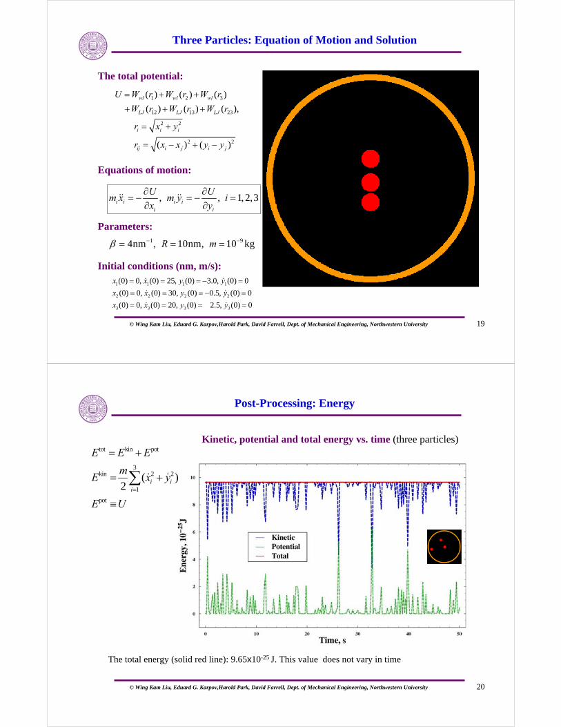
Post-Processing: Energy

Kinetic, potential and total energy vs. time (three particles)

The total energy (solid red line): 9.65x10-25 J. This value does not vary in time

tot kin pot

3kin 2 2

1

pot

( )2 i i

i

E E E

mE x y

E U

=

= +

= +

≡

∑ & &

© Wing Kam Liu, Eduard G. Karpov,Harold Park, David Farrell, Dept. of Mechanical Engineering, Northwestern University 21

Post-Processing: Kinetic Energy, Temperature and Pressure

Averaged kinetic energy vs. time (three particles)

Kinetic energy, and therefore temperature and pressure are due to motion of the particles.

Time averaged kinetic energy of particles is approaching the value

which corresponds to temperature

Note: a low temperature system was chosen in order to observe the real-time atomic motion.

Pressure in the system is due to the radial components of velocities:

kin 253.057 10 JE −= ⋅

25kin

23

1 3.057 100.02K

1.38 10T E

k

−

−

⋅= =

⋅

2 9, cos sin 3.23 10 Parad rad x y

mNP v v v v P

Vγ γ −= = + ⇒ = ⋅

© Wing Kam Liu, Eduard G. Karpov,Harold Park, David Farrell, Dept. of Mechanical Engineering, Northwestern University 22

Post-Processing: Internal Energy

Averaged potential energy vs. time (three particles)

Internal energy is due to interaction of particles with each other and with external constraining fields.

Time averaged potential energy of the system is approaching the value

that gives the internal energy of the system.

250.480 10 JU −= ⋅

© Wing Kam Liu, Eduard G. Karpov,Harold Park, David Farrell, Dept. of Mechanical Engineering, Northwestern University 23

Five Particles: Equations of Motion and Solution

The total potential:

Equations of motion:

Parameters:

Initial conditions (nm, nm/s):

1 2 3 4 5

12 13 14 15

23 24 25

34 35

45

( ) ( ) ( ) ( ) ( )

( ) ( ) ( ) ( )

( ) ( ) ( )

( ) ( )

( )

wl wl wl wl wl

LJ LJ LJ LJ

LJ LJ LJ

LJ LJ

LJ

U W r W r W r W r W r

W r W r W r W r

W r W r W r

W r W r

W r

= + + + ++ + + ++ + ++ ++

, , 1, 2,3, 4,5i i i ii i

U Um x m y i

x y

∂ ∂= − = − =

∂ ∂&& &&

1 94nm , 10nm, 10 kgR mβ − −= = =

1 1 1 1

2 2 2 2

3 3 3 3

4 4 4 4

5 5 5 5

(0) 0, (0) 25, (0) 5.6, (0) 0

(0) 0, (0) 30, (0) 3.0, (0) 0

(0) 0, (0) 20, (0) 0.5, (0) 0

(0) 0, (0) 24, (0) 2.5, (0) 0

(0) 0, (0) 22, (0) 4.9, (0) 0

x x y y

x x y y

x x y y

x x y y

x x y y

= = = − == = − = − == = = − == = − = == = = =

& &

& &

& &

& &

& &

© Wing Kam Liu, Eduard G. Karpov,Harold Park, David Farrell, Dept. of Mechanical Engineering, Northwestern University 24

Post-Processing: Energy

Kinetic, potential and total energy vs. time (five particles)

The total energy (solid red line): 3.66x10-25 J. This value does not vary in time

UE

yxm

E

EEE

pot

iii

kin

potkintot

≡

+=

+=

∑=

5

1

22 )(2

&&

© Wing Kam Liu, Eduard G. Karpov,Harold Park, David Farrell, Dept. of Mechanical Engineering, Northwestern University 25

Post-Processing: Kinetic Energy, Temperature and Pressure

Averaged kinetic energy vs. time (five particles)

Kinetic energy, and therefore temperature and pressure are due to motion of the particles.

Time averaged kinetic energy of particles is approaching the value

which corresponds to temperature

Note: a low temperature system was chosen in order to observe the real-time atomic motion.

JE kin 2510847.2 −⋅=

KEk

T kin 041.01

==

© Wing Kam Liu, Eduard G. Karpov,Harold Park, David Farrell, Dept. of Mechanical Engineering, Northwestern University 26

Post-Processing: Internal Energy

Averaged potential energy vs. time (five particles)

Internal energy is due to interaction of particles with each other and with external constraining fields.

Time averaged potential energy of the system is approaching the value

that gives the internal energy of the system.

JU 2510813.0 −⋅=

© Wing Kam Liu, Eduard G. Karpov,Harold Park, David Farrell, Dept. of Mechanical Engineering, Northwestern University 27

Five Particles in a Rough Wall: Equations of Motion and Solution

The total potential:

Equations of motion:

Parameters:

Initial conditions (nm, nm/s):

1 94nm , 10nm, 10 kgR mβ − −= = =

1 1 1 1

2 2 2 2

3 3 3 3

4 4 4 4

5 5 5 5

(0) 0, (0) 25, (0) 5.6, (0) 0

(0) 0, (0) 30, (0) 3.0, (0) 0

(0) 0, (0) 20, (0) 0.5, (0) 0

(0) 0, (0) 24, (0) 2.5, (0) 0

(0) 0, (0) 22, (0) 4.9, (0) 0

x x y y

x x y y

x x y y

x x y y

x x y y

= = = − == = − = − == = = − == = − = == = = =

& &

& &

& &

& &

& &

wallparticlesLJwallLJ WWWU ++= ∑∑ ,,

The system potential is the sum of the L.J. interactions between the particles, the particles and the wall and a circular wall potential

+ 14 static particles representing the rough wall !

,...3,2,1,, =∂∂

−=∂∂

−= iy

Uym

x

Uxm

iii

iii &&&&

© Wing Kam Liu, Eduard G. Karpov,Harold Park, David Farrell, Dept. of Mechanical Engineering, Northwestern University 28

Five Particles in a Rough Wall: Mathematica Code

Define System Potential, including L.J. Potentials and wall potential, along with simulation parameters

Integrate the equations of motion in time to obtain the trajectories of the particles

© Wing Kam Liu, Eduard G. Karpov,Harold Park, David Farrell, Dept. of Mechanical Engineering, Northwestern University 29

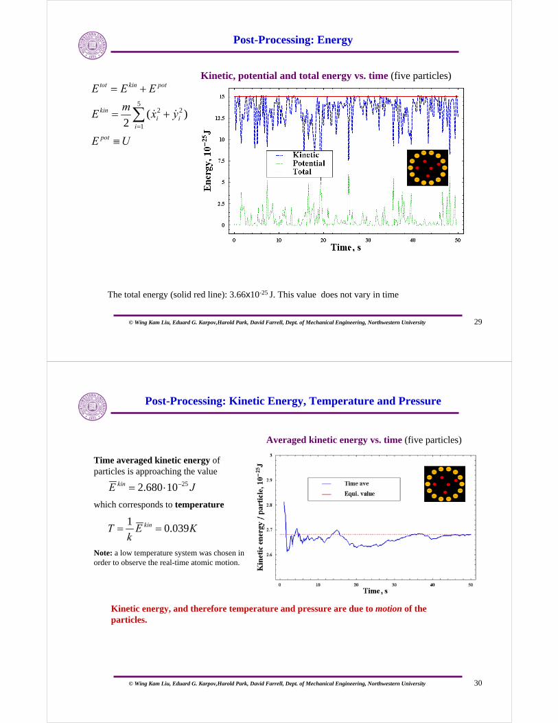
Post-Processing: Energy

Kinetic, potential and total energy vs. time (five particles)

The total energy (solid red line): 3.66x10-25 J. This value does not vary in time

UE

yxm

E

EEE

pot

iii

kin

potkintot

≡

+=

+=

∑=

5

1

22 )(2

&&

© Wing Kam Liu, Eduard G. Karpov,Harold Park, David Farrell, Dept. of Mechanical Engineering, Northwestern University 30

Post-Processing: Kinetic Energy, Temperature and Pressure

Averaged kinetic energy vs. time (five particles)

Kinetic energy, and therefore temperature and pressure are due to motion of the particles.

Time averaged kinetic energy of particles is approaching the value

which corresponds to temperature

Note: a low temperature system was chosen in order to observe the real-time atomic motion.

JE kin 2510680.2 −⋅=

KEk

T kin 039.01

==

© Wing Kam Liu, Eduard G. Karpov,Harold Park, David Farrell, Dept. of Mechanical Engineering, Northwestern University 31

Post-Processing: Internal Energy

Averaged potential energy vs. time (five particles)

Internal energy is due to interaction of particles with each other and with external constraining fields.

Time averaged potential energy of the system is approaching the value

that gives the internal energy of the system.

JU 2510645.0 −⋅=

© Wing Kam Liu, Eduard G. Karpov,Harold Park, David Farrell, Dept. of Mechanical Engineering, Northwestern University 32

Isothermal Example: 1D Lattice with a “Cold” Region

Total number of particles is large.

Interaction between particles is modeled with the two-body harmonic potential:

here, rij = yi – yj is the relative distance between particles i and j in the vertical (y-axis) direction, k – linear interaction coefficient (similar to spring stiffness).

Several atoms in the middle of the chain (between the yellow dashed lines) represent the initially “cold” region. Initial velocities and displacements for these atoms are zero. The remaining atoms have randomly distributed initial velocities and displacements.

21( )

2h ij ijW r kr=

y “Cold” region

© Wing Kam Liu, Eduard G. Karpov,Harold Park, David Farrell, Dept. of Mechanical Engineering, Northwestern University 33

1D Lattice: Equations of Motion and Solution

Number of particles simulated: 50.

Boundary conditions are periodic, so that the coupling between the 50th and 1st particles is established. For a more symmetric view, the simulation shows the 1st particle at both ends of the lattice.

The total potential (the last term is due to periodic boundary conditions):):

Equations of motion:

Parameters:

Initial conditions:

492

1 1 501

1( ) ( ), ( ) ( )

2h i i h h i j i ji

U W y y W y y W y y k y y+=

= − + − − = −∑

, 1, 2,...50ii

Um y i

y

∂= − =

∂&&

21 2110 kg, 10 N/mm k− −= =

middle atoms 22..27 : (0) (0) 0,

other atoms : (0), (0) random within [ 1,1]i i

i i

y y

y y

= =− −

&

&

© Wing Kam Liu, Eduard G. Karpov,Harold Park, David Farrell, Dept. of Mechanical Engineering, Northwestern University 34

Post-Processing: Kinetic Energy and Temperature

Averaged kinetic energy per particle vs. time (for the initially “cold” subsystem)

Time averaged kinetic energy of particles in the “cold” subsystem is approaching the value

which corresponds to temperature

kin 210.286 10 JE −= ⋅

kin

21

23

2

2 0.286 1041.4K

1.38 10

T Ek

−

−

=

⋅ ⋅=

⋅0 100 200 300 400 500

Time, s

0.1

0.2

0.3

0.4

citeniK

ygrene,

01-

12J

Equilibrium value

Time averaged

In contrast to the adiabatic system example, the kinetic energy for the open isothermal subsystem both fluctuates and approaches asymptotically the statistical average.

© Wing Kam Liu, Eduard G. Karpov,Harold Park, David Farrell, Dept. of Mechanical Engineering, Northwestern University 35

Post-Processing: Internal Energy

Averaged potential energy vs. time (“cold” subsystem)

Time averaged potential energy of the “cold” subsystem is approaching the value

that gives the internal energy of the subsystem.

250.480 10 JU −= ⋅

In contrast to the adiabatic system example, the internal energy for the open isothermal subsystem both fluctuates and approaches asymptotically the statistical average.

0 100 200 300 400 500

Time, s

0.5

1

1.5

2

laitnetoP

ygrene,

01-

12J

Internal energy asymp

Time averaged