Demasking the impact of micro–nance - Welcome to the Chair in Macroeconomics!€¦ · ·...

Demasking the impact of micro�nance

Helke Waelde�

November 9, 2011

Abstract

We reconsider data from a randomized control trial study in India. The data

reveal the impact of a microloan program. We extend the often used randomized

impact evaluation and di¤erence-in-di¤erence approach by quantile regression and

the consideration of the quantile treatment e¤ects. The use of additional, more

advanced, evaluation methods allows a more detailed consideration of borrowers at

the lower and at the upper end of the wealth distribution. We �nd a strong negative

and signi�cant time-trend. Furthermore, we observe a negative impact of the provi-

sion of micro�nance loans such that the overall impact is even more negative. This

is particularly well seen for entrepreneurs in the lower and in the higher quantiles.

As we learn that poor entrepreneurs use microloans for consumption, we doubt that

micro�nance is the right instrument for them. The data suggest that providing

microloans for average entrepreneurs, who can hire very poor entrepreneurs, might

be an e¤ective solution for that dilemma.

�Gutenberg School of Management and Economics, University of Mainz, Jakob-Welder-Weg 4, 55128Mainz, Germany, [email protected], www.helke.waelde.com, Phone +49.6131.39-23969, Fax+49.6131.39-25053. We would like to thank Amelie Wuppermann for helpful comments and the Jo-hannes Gutenberg-University for the �nancial support of this paper by a research grant.

1

1 Introduction

The evaluation of treatments is very important and fundamental for the treated and the

not treated. In some cases, especially in the �eld of medicine, it could be life saving or life

destroying. To evaluate the e¤ect of a treatment, we have to apply the treatment, a pill

or something similar, to a group of randomly chosen patients, i.e. the treatment group.

In a perfect setup, we would observe the outcome, the wellbeing of the patient, and turn

back time. Then we observe the same patient when she does not receive the treatment.

After that we would know whether the pill was e¤ective or not. Unfortunately, we are not

able to turn back time. Instead of that we match similar patients and choose at random

which one of them will receive the treatment and which will not. The patients are not

aware of the fact that they did not receive the medicine as they received placebos. As

psychological aspects play an important role in the wellbeing of people, the assumption of

random application of the treatment is essential. Beside the huge insights that scientists

can learn from such an evaluation, we have ethical concerns about this method. How

could we randomly decide who is worth the treatment and who is not? Are we eligible to

make such decision over other people�s live?

However, this method is also applied in other disciplines aside from medicine. In the

development context, we try to evaluate development aid programs with the treatment

evaluation approach. Goldstein and Karlan (2007) and Goldberg and Karlan (2008)

provide an overview of the evaluation of impact for micro�nance. Ideally, we match some

pairs of similarly poor entrepreneurs and randomly o¤er one of them a microloan. The

other poor entrepreneur does not receive an o¤er and continues life without a microloan.

This must not necessarily mean that this person does not receive any loan as there is a

huge mass of informal �nance in developing countries.

The �rst problem arises in the assumption of the randomly distributed treatment.

In micro�nance the treatment is often loans that are given to groups. In many studies,

the borrowers form group themselves. We call this mechanism assortative matching,

�rstly described by Ghatak (1990). Thus, we are not able to randomly choose one target

person for a loan. To solve this problem, we could compare villages. In some villages we

could introduce micro�nance, in others not. But nevertheless, applying the treatment to

randomly chosen villages is not always possible. Micro�nance institutions have limited

resources in �nancial and personal terms. Furthermore, we still face the ethical concerns

mentioned above. To summarize, we see that the treatment is not applied to the same

2

person twice, the application is most of the time not random, and looking at longitude

data, control units often become treated units during the survey time. Therefore, we see

that we have a problem with control groups in micro�nance as the results might be biased

in various ways.

There are many data sets with microdata available for development issues and they are

becoming more and more prevalent. Unfortunately, most of the data lack on a long-term

control group like the World Bank data set used by Khandker (2005), the USAID data

considered by Barnes et al. (2001) and the IFPRI data studied by Behrman (2010). An

unbiased consideration is hard to defend.

Therefore, we ask: Is there a way to evaluate the e¤ect of a treatment more e¤ectively?

We would like to apply di¤erent methods which are commonly used in economics for

evaluating a micro�nance program in India. We start with (i) the simple randomized

impact evaluation and (ii) the di¤erence-in-di¤erence approach by Ashenfelter (1978) and

Ashenfelter and Card (1985). Furthermore, we extend the scope of the methods by (iii)

the quantile regression (Koenker and Basset, 1978) and (iv) the quantile treatment e¤ects

(Firpo, 2007).

We use data from the IFRM-Centre of Micro�nance1 which were also used by Banerjee

et al. (2009). The outstanding characteristic of this data is that the control group remains

untreated over time2. Another much appreciated characteristic of this data set is that

the application of the program was random. Thus, we do not have to handle very harsh

biases. We consider the expenditure of households depending on their participation in

the program. We would like to quantify coe¢ cients and compare their robustness. To

achieve deeper insights we decompose the results into coe¢ cients coming from private

expenditure and coe¢ cients coming from business expenditure.

We �nd a strong negative and signi�cant time-trend and no impact or a negative

impact of the microloan program. Using quantile regression, we learn that especially

the poor entrepreneurs su¤er from a negative impact of the treatment. The average

individual seems to decrease private expenditure when increasing business expenditure

and does not experience any impact from microloans. Entrepreneurs at the upper end

of the distribution have again negative impacts of the treatment when considering the

business expenditure. We state that the micro�nance program has at least no positive

1The data are available on www.ifmr.ac.in.2The micro�nance program from one MFI is not applied to the control group. Unfortunately, other

MFI�s were present in the control villages. However, the level of micro�nance in the control villagesremains signi�cantly lower than in the treated villages (Banerjee et al., 2009).

3

impact on entrepreneurs. We suggest to adjust programs more to �t speci�c groups of

entrepreneurs and their needs.

Compared to Banerjee et al. (2009), we �nd more detailed results from our con-

sideration according to the treatment. Additionally, we are able to extract a negative

time-trend. Furthermore, by using quantile regression, we can �rstly di¤erentiate be-

tween the impact of micro�nance on very poor entrepreneurs and very rich entrepreneurs.

On the other hand, we are only focusing on the impact of the treatment, while Banerjee

et al. (2009) consider also further important variables like gender and age.

Coming back to the control group dilemma, we would like to mention several other

approaches that try to solve the control group problem. Abadie et al. (2010) try to solve

the dilemma by creating arti�cial control groups. However, we still have the problem to

�nd enough similar individuals who live under similar conditions to form such a group.

Todd and Wolpin (2006) �nd a way to evaluate a program without the need for a control

group. They carry out a structural forecast of the impacts of a school subsidy program in

Mexico and compared it to the experimental outcome. The forecast in their model had a

reasonably good result. For completeness we have to mention that there is no comparison

of an ordinary treatment evaluation and a structural estimation in the literature. There-

fore, we can not comment on the results of Todd and Wolpin (2006) at this stage of our

research.

The paper is organized as follows. In section 2, we describe the data used. Section 3

provides information on di¤erent data levels and in section 4, we outline the methods we

use. We then describe the empirical results in section 5 and interpret them in section 6.

We conclude with a short comment in section 7.

2 Survey design

The IFMR-Centre of Micro�nance3 provides comprehensive data from a microloan pro-

gram in Hyderabad, India. The considered program is the microloan program from Span-

dana, a large Indian micro�nance lender. The characteristics of the microloan program

from Spandana4 are

� group-based lending,3www.ifmr.ac.in4www.spandanaindia.com

4

� with a duration of 50 weeks,

� a loan size from Rs 2,000 to Rs 25,000, and

� weekly repayment schedules.

The general loan, Abhilasha, is supposed to �nance small ventures. There are two

subsequent loans. Samruddhi, which is an income generating group loan and Pragathi,

which is o¤ered to entrepreneurs who want to launch a microenterprise. To be eligible for

a loan from Spandana, clients must

(a) be a female,

(b) between 18 and 59 years old,

(c) live for at least one year in the area, and

(d) have an identi�cation and residential proof.

(e) Groups are formed by themselves and

(f) at least 80 % of a group must own their home.

Spandana also o¤ers individual loans, but only to men who have a monthly source

of income. Conditions (b) to (d) also apply to men. As 96,5 % of the borrowers from

Spandana are women, we disregard individual loans. Spandana o¤ers some side-products

like safe drinking water inventions, renewable-energy product portfolios, life-insurance

and new market linkages. But these products are not mandatory to the borrowers5.

At the beginning of the experiment, Spandana selected 120 slums in which they would

like to open branches. Only slums with no pre-existing micro�nance lending schemes

and with potential borrowers that were poor but not at the lowest level of poverty were

selected. Slums with a large amount of construction workers were excluded as they seem

to be more willing to apply for a microloan than other entrepreneurs. The population in

the slums ranges from 46 to 555 households.

After the �rst survey, 16 slums were dropped, as these contained a large number of

migrant-worker households. However, 104 slums remained. These slums were paired

based on their per capita consumption, their fraction of households with debt, and their

5www.spandanaindia.com

5

fraction of households with a business. Then one of these slums was randomly assigned

to the treatment, i.e. Spandana started providing group loans to the borrowers in the

treated areas. The second survey took place at least 12 months after the assignment, but

on average after 15 to 18 months.

In the �rst wave in 2005, the IFMR surveyed 2,800 households living in slums. The

selected households are supposed to have at least one woman between 18 and 55 years,

as the group loans from Spandana mainly target women. The questionnaire requests

information on household composition, education, employment, asset ownership, decision-

making, expenditure, borrowing, saving, and businesses. In 2007 and 2008 the slums were

resurveyed. At this time, information from 6,798 households was collected. The survey

did not intend to resurvey exactly the same households in the slums (Banerjee et al.,

2009).

Summarizing the characteristics of the data set, we see that the assignment of treat-

ment to 52 of the 104 slums was applied randomly and that the control slums remained

untreated over time at least for micro�nance loans from Spandana6.

3 Di¤erent data levels

We will consider the data on two di¤erent levels to obtain driving factors of the changes in

wealth. First we study the data at the slum level in a panel data structure. Afterwards,

we consider the data at the individual level in form of repeated cross-section data.

3.1 Panel data at the slum level

In the data we obtain information on individuals who live in one slum. As we can follow

the slums perfectly over two periods in time we average the values for expenditure of

all individuals in one slum. We therefore obtain two values of expenditure, one for 2005

before the micro�nance program was launched and one for 2007 for each slum when the

program �nished.

A �rst advantage of using panel data methods are more precise standard errors com-

pared to ordinary least square regression (OLS) for pooled data. The OLS seems to

underestimate standard errors and thus t-statistics were overestimated (Cameron and

6Other MFI�s provides microloans in the control area during the time of the survey. But as Banerjeeet al. (2009) argue, the probability to receive a loan was still higher in treated areas than in control areas.

6

Trivedi, 2005). Second, as the treatment is said to be random in our data set we can esti-

mate them in a �xed e¤ects model. As a result, we account for unobserved heterogeneity

between the slums that stays constant over time and might be correlated with regressors.

This problem might appear small in our data set as we have only two periods of time.

The opposite to �xed e¤ects are random e¤ects. We describe unobserved heterogeneity

as random e¤ect when it is independently distributed from the regressors. But following

Cameron and Trivedi (2005), economists regret the possibility of a random e¤ect model

to represent the true model. As a third advantage, we can follow the panel data over time

and learn something about the dynamics of the dependent variable, when assuming no

correlation between the regressors.

To account for the disadvantages of panel data, we suggest a paper by Bertrand et

al. (2004). They �nd that because of serial correlation in repeated panels, the ordinary

standard errors might understate the deviation of the treatment e¤ect and as a result still

overestimate the t-statistics and their respective signi�cance levels. They suggest di¤erent

methods such as block bootstrapping to avoid the problem. It also becomes clear that the

problem arises in data sets which are recorded at more than two points in time. In our

data we are faced with a so called short panel which means we have a large population

but only two periods of time. In short panels, a biased estimation as mentioned above

is unlikely. However, we will report a bootstrap regression as a comparison for each

regression.

3.2 Repeated cross-section data at the individual level

By focusing on panel data, we lose some information on individuals and the structure of

the slum. However, we enrich our consideration by estimating models based on individual

data in a repeated cross-section analysis. We obtain 2; 440 observations in 2005 and 6; 763

observations in 2007. Before obtaining these �nal numbers, we remove missing data. The

treatment variable was missing for 360 individual data out of 2; 800 individual data in

2005. Therefore we had to delete these data. In 2007, all individual data remained.

The advantage coming from repeated cross-section analysis is that we have a larger

number of observations. The problem arising with that is, however, that a repeated cross-

section analysis can lead to inconsistent estimates (Cameron and Trivedi, 2005). To check

the robustness of the estimates, we can not do a �xed e¤ects regression as we do not have

a panel structure here. To solve this problem we form a pseudo panel, where we pool

7

information on slum level (Khandker et al., 2010) to do a �xed e¤ects model regression.

So we obtain robust estimates again. As we do not consider a panel data structure here,

we can report results without bootstrapping estimations. Furthermore, as we consider

many entrepreneurs from each slum, the error terms of the individuals in one slum can be

correlated. The standard errors of these individuals will be clustered to account for the

problem.

4 Di¤erent evaluation methods

As we would like to measure whether the availability of a microloan program has a positive

impact on wealth, we have to identify variables to measure wealth from the data set. As

there is no consistent information about the assets of an individual, we use expenditure

as such. The more an individual is spending, the more wealth the individual is supposed

to have. For a nearer consideration of the data, we allow for a disaggregation of the

expenditure in private expenditure and expenditure for business investments.

A census was taken in India in 2007. Banerjee et al. (2009) �nd that Spandana

borrowers were oversampled in that census. Thus, we have to adjust for the oversampling

by weighting our results, as we only want to obtain the e¤ect of the treatment and do not

claim to re�ect the true model.

4.1 Randomized impact evaluation

As the treatment is said to be randomly assigned to 52 of the 104 slums, the randomized

impact evaluation (RIE) would be the simplest way to evaluate the program. We assume

no selection bias in the data given the random assignment. Usually, the RIE is applied to

cross-section data for the second period in time, only. As a result we observe the impact

after the treatment was applied. This method consists of a t-test or alternately of an

ordinary least square regression (OLS). The regression is given by

lnExpi = �+ �Treati + "i (1)

where i denoted the individual. The expenditure is the dependent variables on the left-

hand side and the assigned treatment is the only explanatory variable on the right-hand

side. We test whether the coe¢ cient � of the treatment variable is signi�cantly di¤erent

for the treated slums and the non-treated slums.

8

4.2 Di¤erence-in-di¤erence approach

To obtain deeper information and to be able to analyze the robustness of the coe¢ cients,

we apply a di¤erence-in-di¤erence approach (DiD). Suppose we consider a correct control

group, selection biases should not be a problem. We consider the di¤erent individuals

or slums at di¤erent periods of time. By using double di¤erences, we remove time-

invariant socioeconomic characteristics that might be di¤erent for the considered slums or

individuals. Starting with the control group, we consider the expenditure of an individual

in 2005 as

E (lnExpit j Treatit = 0; Y earit = 2005) = � (2)

and in 2007 as

E (lnExpit j Treatit = 0; Y earit = 2007) = �+ �Y . (3)

where i denotes the individual and t denotes time. Then we take the �rst di¤erence

E (lnExpit j Treatit = 0; Y earit = 2007)�E (lnExpit j Treatit = 0; Y earit = 2005)

= �Y . (4)

Now we consider the treated group in 2005, i.e. before the treatment, as

E (lnExpit j Treatit = 1; Y earit = 2005) = �+ �T (5)

and in 2007, after the treatment, as

E (lnExpit j Treatit = 1; Y earit = 2007) = �+ �T + �Y + �TY . (6)

We consider the �rst di¤erence as

E (lnExpit j Treatit = 1; Y earit = 2007)�E (lnExpit j Treatit = 1; Y earit = 2005)

= �Y + �TY . (7)

9

Equation (4) and equation (7) give the change in expenditure for the control group and

the treated group. To obtain signi�cant di¤erences in this change we have to take the

second di¤erence as

E[(lnExpit j Treatit = 1; Y earit = 2007)�E (lnExpit j Treatit = 1; Y earit = 2005)]�E[(lnExpit j Treatit = 0; Y earit = 2007)�E (lnExpit j Treatit = 0; Y earit = 2005)]

= �TY . (8)

The resulting coe¢ cient �TY measures the di¤erence caused by the treatment (Imbens

and Wooldridge, 2009). We estimate the coe¢ cient by using

lnExpit = �+ �Y Y earit + �TTreatit + �TY (Treat � Y ear)it + "it (9)

where the expenditure are the dependent variable on the left-hand side and year and

treatment are the dummy variables on the right-hand side. The Y ear is coded with 0 for

2005 and 1 for 2007. The variable Treat is 0 for an individual in the control group and

1 for an individual in the treatment group. The variable Treat � Y ear is 1 if and only ifthe individual is treated and considered in 2007. Otherwise this variable equals 0.

The coe¢ cient �TY is the variable of interest to us. If that coe¢ cient is signi�cant,

there might be a positive or negative impact from the microloan program on the expen-

diture. Furthermore, we look at �Y to analyze whether there is a time-trend in the data

or not. The coe¢ cient �T is expected to be insigni�cant or zero as the treatment is said

to be randomly applied. We weight the results to be able to interpret the results for the

whole population in slums.

4.3 Quantile regression with the DiD approach

The DiD estimation calculates the e¤ect on the average expenditure. By using quantile

regression (QR), we can �nd the e¤ects at di¤erent quantiles of the expenditure distrib-

ution. As a result, we can consider the changes for very poor individuals or slums and

also for very rich individuals or slums, which are caused as a result of using of Spandana

microloans. In contrast to the OLS estimation, the quantile regression minimizes absolute

10

values of errors. The errors were asymmetrically weighted dependent on the quantile we

are about to estimate. The quantile regression estimator b�q is minimizing over �qQN

��q�=PN

i:y�x0i�q��yi � x0i�q��+PN

i:y<x0i�(1� q)

��yi � x0i�q�� (10)

where the absolute error is given by

e = y � x0�q (11)

(Cameron and Trivedi, 2005). The variable q denotes the qth quantile of the distribution.

The �rst term on the right-hand side of equation (10) summarizes the underestimated

errors, and the second term summarizes the overestimated errors. By using this method,

we can see whether the micro�nance program has a positive or negative e¤ect on slums

at the lower level of the distribution of expenditure or at the other end of the distribu-

tion. This estimation is more robust to outliers and the coe¢ cients are consistent under

weaker assumptions than in the OLS estimation (Cameron and Trivedi, 2005). Following

Khandker et al. (2010) we can estimate the coe¢ cients using

lnExpit = �qXit + "qit; Qt (lnExpitjXit) = �qXit; q 2 (0; 1) . (12)

As we would like to concentrate on the e¤ect of the treatment, we apply two variations of

this method to our data set, �rst the quantile regression with DiD approach and secondly

the quantile treatment e¤ects estimation. The �rst approach gives us information on

the impact of the treatment on di¤erent groups at the lower end or upper end of the

distribution of the expenditure. The second one extracts information on the absolute

di¤erence in expenditure between the treated group and the control group in a special

quantile. Taking both methods together, we can draw a clearer picture of the impacts of

the microloan program over the whole distribution.

We follow Athey and Imbens (2006) by estimating a DiD approach using the ad-

vantages of the quantile regression (QDiD) . They show that the distribution of the

counterfactual is given as

QDiDlnExp(q) = lnExpT0 (q) +

�lnExpC1 (q)� lnExpC0 (q)

�. (13)

At �rst the di¤erence in lnExp over time at the qth quantile of the control group is

11

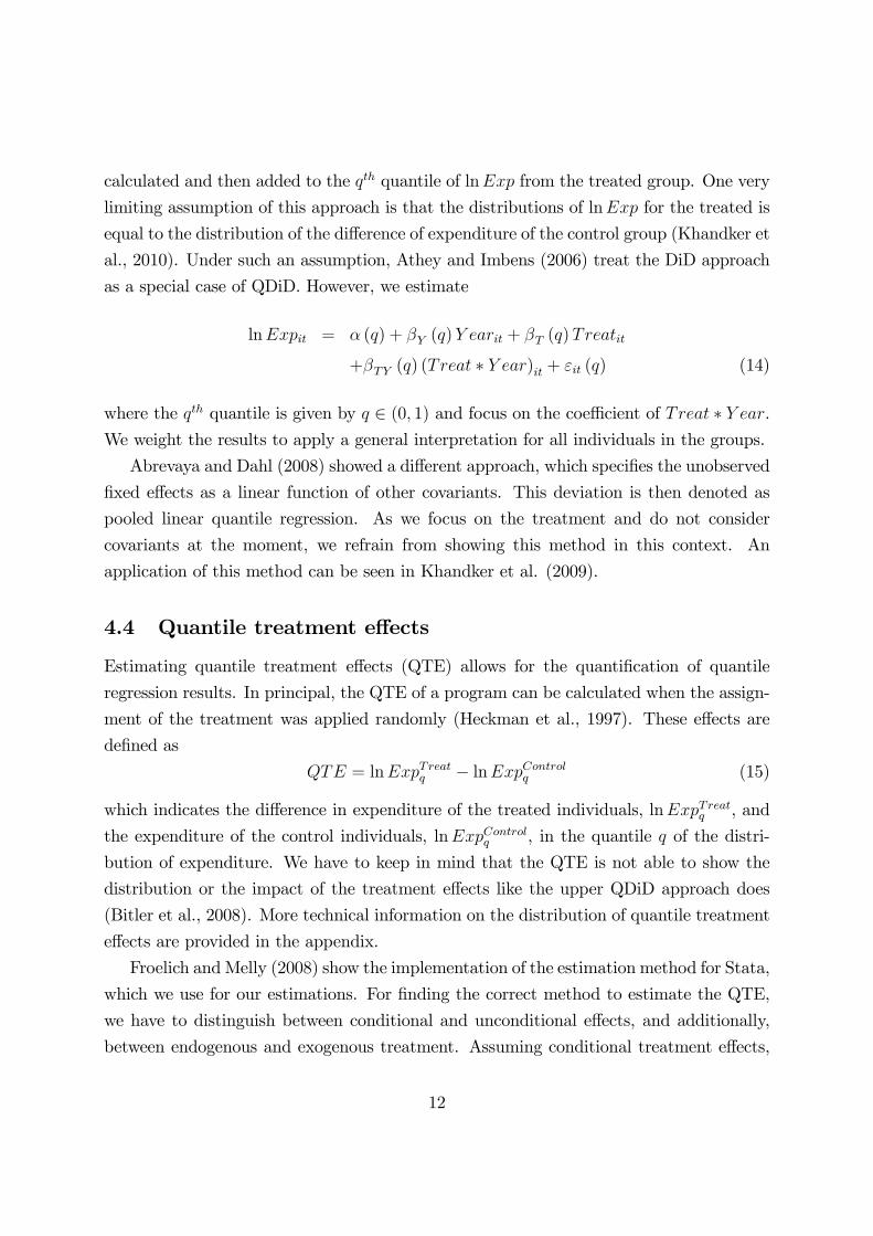
calculated and then added to the qth quantile of lnExp from the treated group. One very

limiting assumption of this approach is that the distributions of lnExp for the treated is

equal to the distribution of the di¤erence of expenditure of the control group (Khandker et

al., 2010). Under such an assumption, Athey and Imbens (2006) treat the DiD approach

as a special case of QDiD. However, we estimate

lnExpit = � (q) + �Y (q)Y earit + �T (q)Treatit

+�TY (q) (Treat � Y ear)it + "it (q) (14)

where the qth quantile is given by q 2 (0; 1) and focus on the coe¢ cient of Treat � Y ear.We weight the results to apply a general interpretation for all individuals in the groups.

Abrevaya and Dahl (2008) showed a di¤erent approach, which speci�es the unobserved

�xed e¤ects as a linear function of other covariants. This deviation is then denoted as

pooled linear quantile regression. As we focus on the treatment and do not consider

covariants at the moment, we refrain from showing this method in this context. An

application of this method can be seen in Khandker et al. (2009).

4.4 Quantile treatment e¤ects

Estimating quantile treatment e¤ects (QTE) allows for the quanti�cation of quantile

regression results. In principal, the QTE of a program can be calculated when the assign-

ment of the treatment was applied randomly (Heckman et al., 1997). These e¤ects are

de�ned as

QTE = lnExpTreatq � lnExpControlq (15)

which indicates the di¤erence in expenditure of the treated individuals, lnExpTreatq , and

the expenditure of the control individuals, lnExpControlq , in the quantile q of the distri-

bution of expenditure. We have to keep in mind that the QTE is not able to show the

distribution or the impact of the treatment e¤ects like the upper QDiD approach does

(Bitler et al., 2008). More technical information on the distribution of quantile treatment

e¤ects are provided in the appendix.

Froelich andMelly (2008) show the implementation of the estimation method for Stata,

which we use for our estimations. For �nding the correct method to estimate the QTE,

we have to distinguish between conditional and unconditional e¤ects, and additionally,

between endogenous and exogenous treatment. Assuming conditional treatment e¤ects,

12

the outcome is dependent on the value of the regressors while for unconditioned e¤ects

the outcome is independent from the regressors. An endogenous treatment is assumed

as long as the treatment is assigned randomly. An exogenous treatment explains the

assignment of the treatment depending on observable characteristics of the individuals

(Froelich and Melly, 2008). However, given di¤erent treatment e¤ects we have to apply

di¤erent estimators as shown in Froelich and Melly (2010). The methods are summarized

in table 1. In our setup, we have unconditional exogenous treatment e¤ects, as the

conditional e¤ects unconditional e¤ectsendogenous treatment Abadie et al. (2002) Froelich and Melly (2008)exogenous treatment Koenker and Bassett (1978) Firpo (2007)

Table 1: Overview over methods to estimate QTE

assignment was random and we can observe characteristics of the individuals. We use the

technique of Firpo (2007) for our estimation.

5 Empirical results

5.1 Panel data at the slum level

5.1.1 Randomized treatment evaluation

As the treatment was said to be randomly assigned, we establish an ordinary least square

estimation (OLS) using the data from 2007 �rst. We weight our results because Spandana

borrowers were oversampled. Weighted results can be interpreted as correct coe¢ cients

for the complete population. Therefore, we regress


where i = 1; :::; 104. We obtain the results in table 2. As the coe¢ cient estimates are

not signi�cant coe¢ cients for the treatment ,we have to be careful in interpreting these

results. We do not observe a direct impact of a micro�nance treatment from Spandana on

slums. However, for this result and other results at the slum level we have to mention that

we consider averaged data. Even if we break down the data set into private expenditure

and business expenditure, we �nd no signi�cant results. Therefore, we take advantage of

13

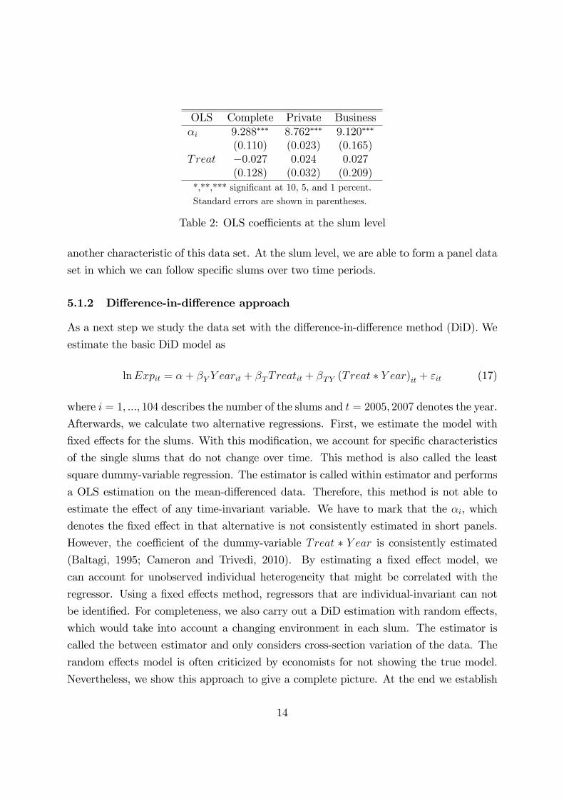
OLS Complete Private Business�i 9:288�� 8:762�� 9:120��

(0:110) (0:023) (0:165)Treat �0:027 0:024 0:027

(0:128) (0:032) (0:209)*,**,*** signi�cant at 10, 5, and 1 percent.

Standard errors are shown in parentheses.

Table 2: OLS coe¢ cients at the slum level

another characteristic of this data set. At the slum level, we are able to form a panel data

set in which we can follow speci�c slums over two time periods.

5.1.2 Di¤erence-in-di¤erence approach

As a next step we study the data set with the di¤erence-in-di¤erence method (DiD). We

estimate the basic DiD model as


where i = 1; :::; 104 describes the number of the slums and t = 2005; 2007 denotes the year.

Afterwards, we calculate two alternative regressions. First, we estimate the model with

�xed e¤ects for the slums. With this modi�cation, we account for speci�c characteristics

of the single slums that do not change over time. This method is also called the least

square dummy-variable regression. The estimator is called within estimator and performs

a OLS estimation on the mean-di¤erenced data. Therefore, this method is not able to

estimate the e¤ect of any time-invariant variable. We have to mark that the �i, which

denotes the �xed e¤ect in that alternative is not consistently estimated in short panels.

However, the coe¢ cient of the dummy-variable Treat � Y ear is consistently estimated(Baltagi, 1995; Cameron and Trivedi, 2010). By estimating a �xed e¤ect model, we

can account for unobserved individual heterogeneity that might be correlated with the

regressor. Using a �xed e¤ects method, regressors that are individual-invariant can not

be identi�ed. For completeness, we also carry out a DiD estimation with random e¤ects,

which would take into account a changing environment in each slum. The estimator is

called the between estimator and only considers cross-section variation of the data. The

random e¤ects model is often criticized by economists for not showing the true model.

Nevertheless, we show this approach to give a complete picture. At the end we establish

14

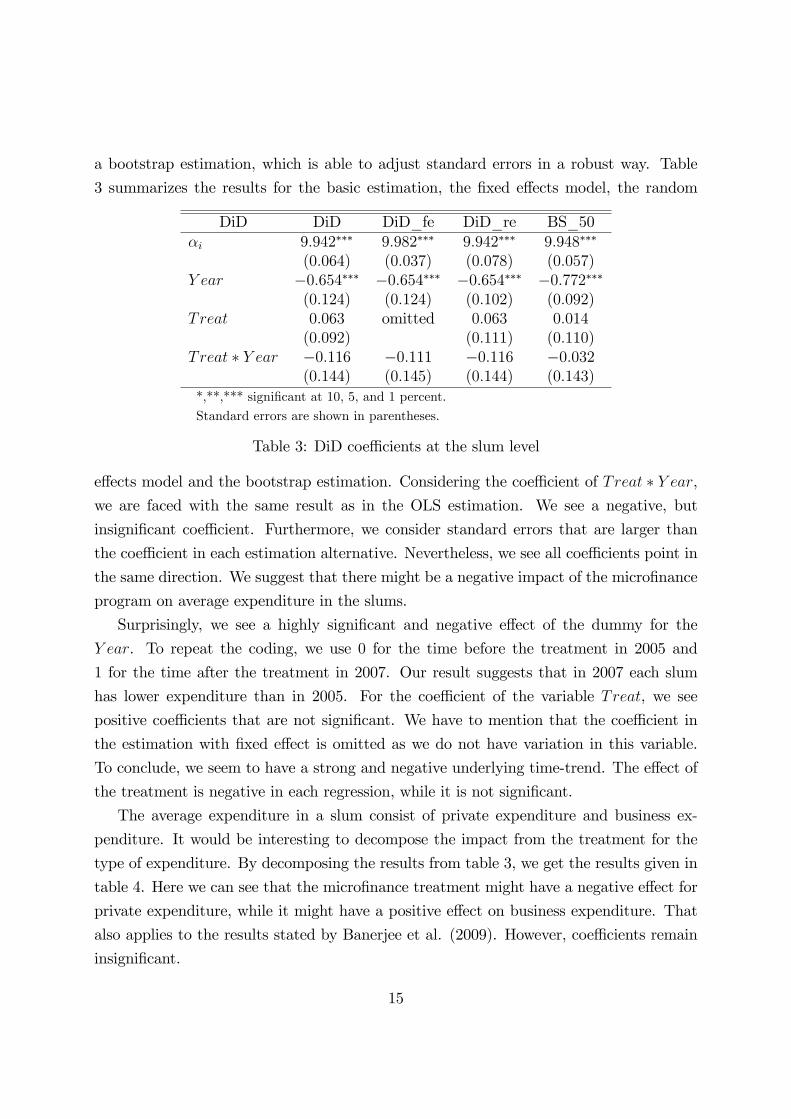
a bootstrap estimation, which is able to adjust standard errors in a robust way. Table

3 summarizes the results for the basic estimation, the �xed e¤ects model, the random

DiD DiD DiD_fe DiD_re BS_50�i 9:942�� 9:982�� 9:942�� 9:948��

(0:064) (0:037) (0:078) (0:057)Y ear �0:654�� 0:654�� 0:654�� 0:772��

(0:124) (0:124) (0:102) (0:092)Treat 0:063 omitted 0:063 0:014

(0:092) (0:111) (0:110)Treat � Y ear �0:116 �0:111 �0:116 �0:032

(0:144) (0:145) (0:144) (0:143)*,**,*** signi�cant at 10, 5, and 1 percent.


Table 3: DiD coe¢ cients at the slum level

e¤ects model and the bootstrap estimation. Considering the coe¢ cient of Treat � Y ear,we are faced with the same result as in the OLS estimation. We see a negative, but

insigni�cant coe¢ cient. Furthermore, we consider standard errors that are larger than

the coe¢ cient in each estimation alternative. Nevertheless, we see all coe¢ cients point in

the same direction. We suggest that there might be a negative impact of the micro�nance

program on average expenditure in the slums.

Surprisingly, we see a highly signi�cant and negative e¤ect of the dummy for the

Y ear. To repeat the coding, we use 0 for the time before the treatment in 2005 and

1 for the time after the treatment in 2007. Our result suggests that in 2007 each slum

has lower expenditure than in 2005. For the coe¢ cient of the variable Treat, we see

positive coe¢ cients that are not signi�cant. We have to mention that the coe¢ cient in

the estimation with �xed e¤ect is omitted as we do not have variation in this variable.

To conclude, we seem to have a strong and negative underlying time-trend. The e¤ect of

the treatment is negative in each regression, while it is not signi�cant.

The average expenditure in a slum consist of private expenditure and business ex-

penditure. It would be interesting to decompose the impact from the treatment for the

type of expenditure. By decomposing the results from table 3, we get the results given in

table 4. Here we can see that the micro�nance treatment might have a negative e¤ect for

private expenditure, while it might have a positive e¤ect on business expenditure. That

also applies to the results stated by Banerjee et al. (2009). However, coe¢ cients remain

insigni�cant.

15

DiD Complete Private Business�i 9:942�� 9:798�� 8:823��

(0:078) (0:061) (0:178)Y ear �0:654�� 1:036�� 0:297

(0:102) (0:062) (0:201)Treat 0:063 0:084 �0:157

(0:111) (0:088) (0:249)Treat � Y ear �0:116 �0:072 0:140



Table 4: Decomposed DiD coe¢ cients at the slum level

Considering the coe¢ cient of Y ear, we see that it is signi�cantly negative for private

expenditure and insigni�cant and positive for business expenditure. We believe the time

trend e¤ects the private expenditure more than the business expenditure. Considering

the variable Treat, we can not observe a signi�cant coe¢ cient for private expenditure and

for business expenditure.

5.1.3 Quantile regression with the DiD approach

As our estimations above are based on averaged data, it might be useful to split the

consideration to convey the �hidden�information. Therefore, we extend the consideration

of Banerjee et al. (2009) and use the method of quantile regression. A slum contains all

kinds of entrepreneurs ranging from very poor to very rich. It is not very likely that each

slum consists of the same distribution of wealth. Rather, we expect to �nd some very

poor slums and some wealthier slums over the whole data set. Quantile regression gives

us an instrument to consider impacts of the treatment on each quantile of the distribution

separately. First we consider poor slums at the 5% quantile, then the average slums at the

50% quantile and �nally the richest slums at the 99% quantile. We do so by estimating

lnExpit = � (q) + �Y (q)Y earit + �T (q)Treatit + �TY (q) (Treat � Y ear)it + "it (18)

where i = 1; :::; 104 describes the number of the slums and q denotes the considered

quantile. To account for the possible biases in standard errors, we refer to the bootstrap

estimation for each quantile. In general, we see that the bias is not large, but for some

coe¢ cients signi�cance levels change. Table 5 illustrates the obtained results. First we

16

QDiD QDiD_05 BS_05 QDiD_50 BS_50 QDiD_99 BS_99�i 8:979�� 8:979�� 9:948�� 9:948�� 10:902�� 10:902��

(0:087) (0:189) (0:071) (0:057) (0:011) (0:103)Y ear �0:251� �0:251 �0:772�� 0:772�� 3:319�� 3:319

(0:122) (0:196) (0:101) (0:092) (0:016) (1:995)Treat 0:323� 0:323 0:099 0:014 0:452�� 0:452�

(0:130) (0:223) (0:101) (0:110) (0:016) (0:199)Treat � Y ear �0:378� �0:407� �0:113 �0:032 �3:808�� 3:808

(0:177) (0:128) (0:143) (0:143) (0:023) (2:059)*,**,*** signi�cant at 10, 5, and 1 percent. Standard errors are shown in parentheses.

Table 5: Comparison of QR coe¢ cients at the slum level

consider the coe¢ cient of Treat � Y ear. We emphasize that this coe¢ cient measuresthe e¤ect for treated slums after treatment. We learn that the results become more

interesting and signi�cant. We �nd negative impacts of the treatment for very poor slums

and for very rich slums. At the 99% quantile, the coe¢ cient is not signi�cant when we

apply the bootstrapping adjustment of the standard errors. That might by caused by

the high variation at the upper end of the distribution. Furthermore, this could be due

to the fact that we do not have enough observations at this quantile to obtain robust

estimations. However, for poor slums the result remains signi�cant. We learn that the

micro�nance program seems to have a negative e¤ect on very poor slums that participate

in the treatment compared to poor slums that did not have the chance to participate in

the micro�nance program. For the 50% quantile, the coe¢ cient for Treat � Y ear is notsigni�cant.

Considering the other coe¢ cients in the 5% quantile and the 50% quantile, we can

not see a unique direction. For the poor slum and the average slum, the coe¢ cient

for Y ear is signi�cantly negative. We suggest that all slums have lower expenditure in

2007. We would like to mention that the coe¢ cient for Treat is positive for poor slums.

That suggests that in these quantile the treatment might not be completely randomized.

Together with our results for the combined coe¢ cient of Treat � Y ear, we propose thatpoor slums are faced with a signi�cantly negative time-trend and a negative impact from

the micro�nance program. Average slums are faced with the negative time-trend, but

have no impact from the treatment at all.

For the 99% quantile, the coe¢ cients of Y ear is positive, which means that rich slums

seems to spend more over time. The coe¢ cient of Treat is also positive and signi�-

17

cant, which would support the suggestion made above that treatment was not completely

randomized in the higher quantiles, too. However, we observe that the treatment e¤ect

coe¢ cient Treat �Y ear points in the opposite direction at a high signi�cance level. Thatwould suggest that a participation in the program has a negative impact for rich slums.

As we see that the signi�cant coe¢ cient becomes insigni�cant when using bootstrapping

methods, we have to be careful in interpreting this result.

We obtain an overview of all quantiles by looking at �gure 1. The dashed line depicts

10.

005

.00

0.00

5.00

ty

0 .2 .4 .6 .8 1Quantile

Figure 1: Comparison of Treat � Y ear for DiD and QR at the slum level

the DiD estimator and the dotted lines show the 10% con�dence interval. The straight

line illustrates the quantile regression estimator while the grey area around it gives the

con�dence interval. We witness a more precise estimator in the QDiD, whereas it stays

in the con�dence interval of the DiD estimation up to the highest quantiles. Therefore,

the QDiD does not contradict the DiD. At the end we see a strong negative outlier, which

repeats the estimation we interpreted above. However, as the con�dence interval increases

at the upper quantile, we will not interpret this result.

18

In the following, we decompose the results into e¤ects from only private expenditure

and from only business expenditure to compare the results and extract the driving forces.

A comparison of the coe¢ cients of the complete model, only private expenditure and only

business expenditure, is shown in table 6. We consider only the coe¢ cient of Treat�Y ear.

Treat � Y ear Complete BS Private BS Business BSQuantile 0.05 �0:378� �0:407� �0:369� �0:377� 0:635 0:635

(0:177) (0:128) (0:149) (0:174) (1:243) (0:887)Quantile 0.50 �0:113 �0:032 �0:008 �0:037 �0:146 �0:142

(0:143) (0:143) (0:118) (0:108) (0:297) (0:294)Quantile 0.99 �3:808�� 3:808 �0:613�� 0:613� �2:667�� 2:667

(0:023) (2:059) (0:006) (0:247) (0:075) (2:231)*,**,*** signi�cant at 10, 5, and 1 percent. Standard errors are shown in parentheses.

Table 6: Decomposition of QR coe¢ cients at the slum level

The given results suggest that treated slums are worse o¤ over nearly all quantiles when

we look at private expenditure or business expenditure. We �nd signi�cantly negative

results for the very poor slums for private expenditure and for all expenditure, while the

coe¢ cient for business expenditure is not signi�cant in the bootstrap estimation. For

average slums, the results are negative but not signi�cant. At the upper end, we see that

microloans have a negative impact on private expenditure. Standard errors are too high

to interpret the results at the other columns. We learn more about the e¤ects caused

by private expenditure or by business expenditure overall quantiles when looking at the

decomposed pictures in table 7. We have to pay attention to the di¤erent scaling on the

y-axis. The scaling in the left �gure is much smaller than in the right �gure. That suggests

that the e¤ects from business expenditure are larger in range. For private expenditure,

the QDiD estimator is signi�cantly lower and exceeds the con�dence interval of the DiD

estimator for poor slums and rich slums. This supports the negative coe¢ cients in our

estimation. In the right picture, we see the business estimators for DiD and QDiD. We

learn that the treatment might have a positive e¤ect for very poor slums as the estimator

exceeds the con�dence interval of the DiD estimator. Furthermore, we become more

sensitive to the e¤ect on the rich slums as the estimator also breaks out of the con�dence

interval here .

19

Private Business

1.0

00

.50

0.00

0.50

ty

0 .2 .4 .6 .8 1Quantile

6.0

04

.00

2.0

00.

002.

004.

00ty

0 .2 .4 .6 .8 1Quantile

Table 7: Private expenditures and business expenditures at the slum level

5.1.4 Quantile treatment e¤ects

Quantile treatment e¤ects (QTE) are an interesting instrument to quantify the di¤erence

between a treatment group and a control group without distortion of strong underlying

trends. Table 8 illustrates the unconditional exogenous treatment e¤ects. Here we �nd

lnExpTreatq � lnExpControlq Complete Private BusinessQuantile 0.05 0:048 �0:022 �0:616Quantile 0.50 �0:196 0:138 0:107Quantile 0.99 0:233 0:296 �0:491

Table 8: QTE at the slum level

that for very poor people the overall e¤ect should be positive, while the decomposed

e¤ects are negative. This might be caused by the averaging of the data. Poor slums

are not increasing their expenditure at all. Slums in higher quantiles of the distribution

seem to be able to gain positive e¤ects from the possibility of participating in a group as

they increase private expenditure or both types of expenditure. The e¤ect states that the

rich slums are not better o¤ because they are able to participate in a microloan program

when considering business expenditure. Overall the e¤ects are ambiguous. We will come

back to this in the next section, when we consider individual data to obtain more robust

information and compare the individual results to the results from the slum level.

20

5.2 Repeated cross-section data at the individual level

5.2.1 Randomized treatment evaluation

In the following section, we repeat our estimations but change the basis of the underlying

data. We use individual, repeated cross-section data. We have 2; 440 observations in 2005

and 6; 763 observations in 2007. As a �rst step we conduct an OLS estimation. Therefore

we regress


where i = 1; :::; 9; 203. We estimate the expenditure as a complete sum, and also decom-

posed as private expenditure only and business expenditure only. We cluster the data

at the slum level to account for correlation of errors of individuals in the same slum and

weight the results to be able to interpret the results for the whole population. The results

are summarized in table 9. We observe no signi�cant coe¢ cients for Treat. When decom-

OLS Complete Private Business�i 8:781�� 8:589�� 7:021��

(0:028) (0:024) (0:129)Treat 0:029 0:015 0:155



Table 9: OLS coe¢ cients at the individual level

posing the results, we do not obtain signi�cant results. The coe¢ cients remain positive.

In the next sections we will apply more advanced methods to quantify the impact and be

able to compare individual results to the aggregate result considered above at the slum

level.

5.2.2 Di¤erence-in-di¤erence estimation

We apply the DiD method at repeated cross-section data. The interpretation of the

coe¢ cients remains. We estimate


where i = 1; :::; 9; 203 describing the number of the individuals. As we do not obtain panel

data, we have to take care of the robustness of the coe¢ cients. Therefore, we cluster error

21

terms of the individuals in each slum and weight results again. Furthermore, we are not

able to obtain a �xed e¤ects model at the individual level. However, we can use the

slums as a basis for the �xed e¤ect. Table 10 summarizes the results. We do not �nd

DiD DiD DiD_fe (on slum)�i 9:461�� 9:949��

(0:038) (0:023)Y ear �0:680�� 0:685��

(0:042) (0:042)Treat 0:088 omitted

(0:055)Treat � Y ear �0:077 �0:025

(0:061) (0:063)*,**,*** signi�cant at 10, 5, and 1 percent.


Table 10: DiD coe¢ cients at the individual level

a signi�cant coe¢ cient for Treat � Y ear. All coe¢ cients for Y ear are signi�cant andnegative. All individuals reduce their expenditure from 2005 to 2007. When we consider

the coe¢ cient of Treat we can not �nd signi�cant coe¢ cients.

Decomposing the result might shed some light on the underlying mechanisms. We

compare results from all expenditure to only private expenditure and only business ex-

penditure in table 11. We learn that all coe¢ cients point in the same direction and seem

DiD Complete Private Business�i 9:461�� 9:370�� 7:731��

(0:038) (0:036) (0:154)Y ear �0:680�� 0:781�� 0:710��

(0:042) (0:037) (0:172)Treat 0:096 0:085 0:228

(0:055) (0:049) (0:217)Treat � Y ear �0:067 �0:082 �0:133



Table 11: Decomposed DiD coe¢ cients at the individual level

to support the interpretation made at the slum level, even if they are insigni�cant. We

do not �nd strong di¤erences between private expenditure and business expenditure.

22

5.2.3 Quantile regression with the DiD approach

By studying single quantiles of the distribution, we are able to obtain the impact of the

program for the very poor individuals at the lower end, for average individuals, and for

richer individuals at the upper end. We estimate

lnExpit = � (q) + �Y (q)Y earit + �T (q)Treatit + �TY (q) (Treat � Y ear)it + "it (21)

where i = 1; :::; 9; 203 describes the number of the slums and q gives the quantile. Table

12 summarizes the obtained results. The big picture remains. We consider negative,

QDiD QDiD_05 QDiD_50 QDiD_99�i 8:300�� 9:308�� 12:320��

(0:038) (0:022) (0:963)Y ear �0:526�� 0:636�� 1:053

(0:045) (0:025) (1:133)Treat 0:131�� 0:072� 0:339

(0:054) (0:031) (1:367)Treat � Y ear �0:107 �0:054 �0:082



Table 12: Comparison of QR coe¢ cients at the individual level

mostly signi�cant coe¢ cients for Y ear, positive coe¢ cients for Treat, and negative but

not signi�cant coe¢ cients for the combined variable Treat � Y ear. The negative time-trend seems to be supported again. Individuals reduce expenditure from 2005 to 2007.

We observe signi�cant positive coe¢ cients for Treat, which should not appear when the

application of the treatment is randomized. Furthermore, we learn that we can not

interpret the treatment e¤ect. Therefore, we summarize that we can not �nd an impact

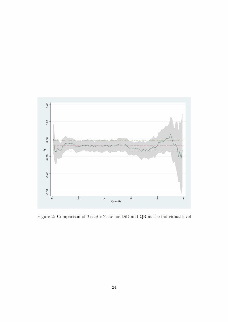
on the microloan program. The coe¢ cients over all quantiles are graphically shown in

�gure 2. The dashed line shows the DiD coe¢ cient and the dotted line depicts the

90% con�dence interval. The straight line shows the quantile regression coe¢ cients for

Treat � Y ear and the grey area the associated con�dence interval. At the lower end andthe upper end of the distribution, we �nd quantile regression coe¢ cients for Treat�Y earwhich exceed the con�dence interval of the DiD estimation. However, as coe¢ cients did

23

0.6

00

.40

0.2

00.

000.

200.

40ty

0 .2 .4 .6 .8 1Quantile

Figure 2: Comparison of Treat � Y ear for DiD and QR at the individual level

24

not appear to be signi�cant for all quantiles, we will not interpret this as a strong evidence

here. For the average quantile, DiD estimation seems to provide good results.

For further insights, we decompose the expenditure in private expenditure and in

business expenditure. We show the coe¢ cient of the combined variable Treat � Y earin table 13. We �nd that all coe¢ cients are not signi�cant, except the coe¢ cients for

Treat � Y ear Complete Private BusinessQuantile 0.05 �0:107 �0:100 �0:511��

(0:063) (0:064) (0:000)Quantile 0.50 �0:054 �0:049 0:086

(0:036) (0:031) (0:327)Quantile 0.99 �0:082 �0:142 0:061



Table 13: Decomposition of QR coe¢ cients at the individual level

very poor business expenditure. That might be a sign that poor entrepreneurs reduce

their business expenditure to secure their daily private consumption. For the average

individuals and the rich individuals, we see positive impact on business expenditure.

We interpret this result such that the individuals above the very poor quantile in the

distribution increase business expenditure while perhaps reducing private expenditure.

They might be able to do so, as they have su¢ cient assets to cover the requirements of

everyday life. Nevertheless, because of small signi�cance levels, we have to be careful in

interpretation. Table 14 shows the quantile regression of private expenditure on the left

side and the business expenditure on the right side. Considering private expenditure, we

�nd that there might be a negative impact overall as described above. Furthermore, we

see that for very poor individuals and for rich individuals, the negative results are stronger

than estimated in the DiD estimation. Considering the business expenditure on the right

side, we do not see much outliers, except the ones at the lower end of the distribution.

That could state that for individuals who become rich enough to launch a business, the

impact might be positive, while for all others the impact seems to not appear or be slightly

negative.

25

Private expenditure Business expenditure

0.6

00

.40

0.2

00.

000.

200.

40ty

0 .2 .4 .6 .8 1Quantile

2.0

00.

002.

004.

00ty

0 .2 .4 .6 .8 1Quantile

Table 14: Private expenditures and business expenditures at the individual level

5.2.4 Quantile treatment e¤ects

The QTE help us to extract the direct di¤erence between the treatment group and the

control group. Table 15 illustrates the unconditional exogenous treatment e¤ects. The

lnExpTreatq � lnExpControlq Complete Private BusinessQuantile 0.05 �0:020 0:016 0Quantile 0.50 0:026 �0:003 0:050Quantile 0.99 0:322 0:137 0:462

Table 15: QTE at the indivdidual level

treatment e¤ects measure the quantitative di¤erence. By doing so, the method weakens

the underlying positive or negative trends. We see that over all expenditure, the very poor

people are not better o¤when o¤ered a microloan program. Considering the decomposed

e¤ects, the private expenditure increases while nothing happened on the business side.

Also, here we see support for the statement that very poor people do not launch a business

or increase their business expenditure. For the average individual, we see a positive

treatment e¤ect. Decomposing the overall e¤ect we �nd a negative e¤ect on private

expenditure and a positive on business expenditure. Individuals are able to reduce private

expenditure for business expenditure by participating in a microloan without impacting

on the everyday life consumption. For rich individuals, microloans o¤er the possibility to

increase both kinds of expenditure. Compared to the averaged results at the slum level,

we �nd a positive impact here for rich entrepreneurs and their business expenditure. We

26

did not extract a similar outcome above.

To summarize, we see that microloans do not seem to have a positive impact even

when considered independently from the underlying trend. Especially poor entrepreneurs

and very rich individuals seem to experience a negative impact as a result of the microloan

program of Spandana. One could construct a pseudo panel with the individual data and

control the results. As we do not expect a signi�cant change, we leave this consideration

for further work.

6 Micro�nance ampli�es the negative time-trend

Considering OLS regressions for slums, we �nd that all coe¢ cients are not signi�cant. The

coe¢ cient for all expenditure is negative. In the individual consideration, all coe¢ cients

are positive but not signi�cant, either. OLS estimations might suggest that the possibility

of obtaining a microloan has a negative impact at the slum level and a positive impact at

the individual level.

Using the advantages of our data, in particular the panel structure at the slum level,

we �nd negative but not signi�cant coe¢ cients for the combined variable in the DiD

approach. Furthermore, we learn that a negative trend in the data might exist, as for this

and all the following regressions, the coe¢ cients for the time-variable are highly signi�cant

and negative. The treatment e¤ect is negative but not signi�cant at the slum level. At

the individual level, the treatment e¤ect is negative and the time-trend highly signi�cant

negative. Therefore, the individual DiD approach provides us with the same information

as the estimations at the slum level. We �nd (i) a strong negative time-trend, and (ii) a

negative treatment e¤ect. Decomposing the results in private expenditure and business

expenditure reveals no new information.

As OLS or DiD regressions estimate one average coe¢ cient for the complete range of

the distribution of expenditure, we consider quantile estimates to obtain speci�c impacts

for very poor slums or entrepreneurs and rich entrepreneurs or slums. At the slum level, we

�nd a signi�cant negative impact from the microloan program on very poor slums and rich

slums. The treatment e¤ect is negative. Correcting the standard errors by bootstrapping

shows that standard errors are heavily underestimated for the high quantile. Furthermore,

we �nd signi�cant coe¢ cients for the treat variable, which would cast doubts on the

randomization of the experiment. When considering the individual data, we see evidence

for the �ndings in the slums for very poor people. For richer entrepreneurs, we can not

27

�nd signi�cant results for the treatment variable while it remains negative. To conclude,

we see that at the lower end of the distribution and at the upper end of the distribution

the impact of micro�nance is negative.

When decomposing the e¤ects we �nd that very poor slums and individuals have

negative e¤ects on both kinds of expenditure. At the slum level, the picture remains the

same for the other quantiles. However, considering the individual data we �nd a decrease

in private expenditure while business expenditure increases. This might suggest that

microloans boost the businesses of individuals. A further interpretation might be that

individuals shift their expenditure into business when not facing daily surviving anymore.

This result for richer individuals was also found by Banerjee et al. (2009).

At the end, we look at quantile treatment e¤ects to consider the quantitative impact

of the opportunity to participate in a program. Here we �nd that the treated group is

better o¤ when in higher quantiles. At the slum level, we have to mention that for slums

at the upper end of the distribution the treatment might have a negative impact on their

business expenditure. At the individual level, we �nd that the poor entrepreneurs can

not gain from the treatment, whereas richer might be able. It also comes to our attention

that entrepreneurs that are accumulating more than a certain level of wealth shift private

expenditure into business expenditure.

7 Concluding comments

Overall, we state that we �nd negative, but mostly insigni�cant impact of the microloan

program. Furthermore, we see a strong negative time-trend over all data. Looking deeper

into the results, we �nd that very poor entrepreneurs are more heavily faced with the

negative time-trend and additionally, micro�nance has a negative impact. Average entre-

preneurs seems to be una¤ected by microloans at all. For entrepreneurs at the upper end,

we �nd a negative impact for business expenditure. We suggest to adjust programs more

to speci�c groups of entrepreneurs and their needs. As we also see that poor entrepreneurs

use the microloan for consumption, we doubt that micro�nance is the right instrument

for them. Finding employment could be the right way for very poor entrepreneurs. We

propose that microloans given to more advanced entrepreneurs, who can hire very poor

entrepreneurs, could be an e¤ective solution for that dilemma.

We have to mention that the negative line that is drawn with this consideration can

have many sources. The most obvious might be the short period of the survey. We have

28

only 15 to 18 months between the �rst round and the second round. Furthermore, we see

strong corrections in the standard errors when using bootstrapping methods. Therefore,

we have to be careful especially in the higher quantile with overstating the results.

Further research could apply the quantile regression to similar data sets. Additionally,

we found out that a third survey round should be available soon. With this we should

be able to extend the consideration. While we can obtain an impact of a treatment

with these methods, we can not extract the drivers of this model. For that, one could

use another method. Todd and Wolpin (2006) use a structural estimation method and

�nd key mechanisms and more e¤ective ways for implementing the treatment. Another

advantage of a structural estimation would be that we do not need control groups for

evaluating the impact of a program. A question not yet put forward in the literature is

how equivalent a DiD approach would be to a structural estimation when it comes to the

robustness of the results. Such a comparison could lead to a new and e¤ective method

for evaluating the impact of programs and extracting the mechanisms behind them at the

same time.

29

8 Appendix

Derivation of quantile treatment e¤ects

Technically, we see that QTE�s are derived from the marginal distributions

FT (lnExp) � Pr[lnExpTi � y]andFC (lnExp) � Pr[lnExpCi � y] (22)

where y denotes the individual expenditure. Following Khandker et al. (2010) these

distributions are known. They argue that assuming the de�nition of the qth quantile from

the distribution Ft (lnExp) ; t = fT;Cg is given as

lnExpt (q) � inf[Y : Ft (lnExp) � q] (23)

the treatment e¤ect for the qth quantile is just the di¤erence in the quantiles of the two

marginal distributions (Khandker et al., 2010, p.125). However, to express the di¤erences

in that way, strong limiting assumptions about the joint distribution of the two marginal

distributions have to be made (see Bitler et al., 2008).

30

References

Abadie, A., J. Angrist, and G. Imbens (2002): �Instrumental variables estimates of

the e¤ect of subsidized training on the quantiles of trainee earnings,�Econometrica, 70

(1), 91�117.

Abadie, A., A. Diamond, and J. Hainmueller (2010): �Synthetic control maeth-

ods for comparative case studies: Estimating the e¤ect of Californis�s tobacco control

program,�Journal of the American Statistical Association, 105 (490), 493�505.

Abrevaya, J., and C. M. Dahl (2008): �The e¤ects of birth inputs on birthweight:

Evidence from quantile estimation on panel data.,�Jorunal of Business and Economic

Statistics, 26 (4), 379�97.

Ashenfelter, O. (1978): �Estimating the e¤ect of training programs on earnings,�

Review of Economics and Statistics, 6 (1), 47�57.

Ashenfelter, O., and D. Card (1985): �Using longitudinal structure of earnings to

estimate the e¤ect of training programs,�Review of Economics and Statistics, 67 (4),

648�60.

Athey, S., and G. Imbens (2006): �Identi�cation and inference in nonlinear di¤erence-

in-di¤erence models.,�Econometrica, 74 (2), 431�97.

Baltagi, B. H. (1995): Econometric analysis of panel data. John Wiley & Sons.

Banerjee, A. V., E. Duflo, R. Glennerster, and C. Kinnan (2009): �The miracle

of micro�nance? Evidence from a randomized evaluation,�Centre for Micro Finance,

IFMR Research Working Paper Series No. 31.

Barnes, C., E. Keogh, and N. Nemarundwe (2001): �Micro�nance program clients

and impact: An assessment of Zambuko Trust, Zimbabwe.,�AIMS Report, USAID.

Behrman, J. R. (2010): �The international Food Policy Reserach Institute (IFPRI) and

the Mexican PROGRESA anti-poverty and human resource investment conditional

cash,�World Development, 38 (10), 1473�85.

Bertrand, M., E. Duflo, and S. Mullainathan (2004): �How much should we

trust di¤erence-in-di¤erence estimates?,� The Quarterly Journal of Economics, 119

(1), 249�75.

31

Bitler, M. P., J. B. Gelbach, and H. W. Hoynes (2008): �Distributional impacts

of the self-su¢ ciency project.,�Journal of Public Economics, 92 (3-4), 748�65.

Cameron, A. C., and P. K. Trivedi (2005): Microeconometrics: methods and appli-

cations. Cambridge University Press.

(2010): Microeconometrics using Stata. Stata Press.

Firpo, S. (2007): �E¢ cient semiparametric estimation of quantile treatment e¤ects,�

Econometrica, 75 (1), 259�76.

Froelich, M., and B. Melly (2008): �Unconditional quantile treatment e¤ects under

endogeneity,�IZA discussion paper No. 3288.

(2010): �Estimation of quantile treatment e¤ects with Stata,�The Stata Journal,

10 (3), 423�457.

Ghatak, M. (1999): �Group lending, local infomation and peer selection,� Journal of

Development Economics, 60 (1), 27�50.

Goldberg, N., and D. Karlan (2008): �Impact of credit: How to measure impact,

and improve operations too,�Financial Access Initiative.

Goldstein, M., and D. Karlan (2007): �Impact evaluation for micro�nance,�The

World Bank, Doing Impact Evaluation, 7.

Heckman, J. J., J. Smith, and N. Clements (1997): �Making the most out of

programme evaluations and social experiments: Accounting for heterogeneity in pro-

gramme impacts.,�Review of Economic Studies, 64 (4), 487�535.

Imbens, G. W., and J. M. Wooldridge (2009): �Recent developments in the econo-

metrics of program evaluation,�Journal of Economic Literature, 47 (1), 5�86.

Khandker, S. R. (2005): �Micro�nance and poverty: evidence using panel data from

Bangladesh,�The World Bank Economic Journal, 19 (2), 263�86.

Khandker, S. R., Z. Bakht, and G. B. Koolwal (2009): �The poverty impact of

rural roads: Evidence from Bangladesh.,�Economic Development and Cultural Change,

57 (4), 685�722.

32

Khandker, S. R., G. B. Koolwal, and H. A. Samad (2010): Handbook on impact

evaluation: quantitative methods and practices. The World Bank.

Koenker, R., and G. J. Bassett (1978): �Regression quantiles,�Econometrica, 46

(1), 33�50.

Todd, P. E., and K. I. Wolpin (2006): �Assessing the impact of a school subsidy

program in Mexico: Using a social experiment to validate a dynamic behavioral model

of child schooling and fertility,�The American Economic Review, 96 (5), 1384�1417.

33

Demasking the impact of micro–nance - Welcome to the Chair in Macroeconomics!€¦ · ·...

Documents

Transcript of Demasking the impact of micro–nance - Welcome to the Chair in Macroeconomics!€¦ · ·...