Demand Forecasting II: Evidence-Based Methods and Checklists

J. Scott Armstrong1

Kesten C. Green2

Working Paper 89-clean

May 24, 2017

This is an invited paper. Please send us your suggestions on experimental evidence that we have overlooked. In particular, the effect size estimates for some of our findings have surprised us, so we are especially interested to learn about experimental evidence that runs counter to our findings. Please send relevant comparative studies that you—or others— have done by June 10. We have a narrow window of opportunity for making revisions. Also let us know if you would like to be a reviewer.

1 The Wharton School, University of Pennsylvania, 747 Huntsman, Philadelphia, PA 19104, U.S.A. and Ehrenberg-Bass Institute, University of South Australia Business School: +1 610 622 6480 F: +1 215 898 2534 armstrong@wharton.upenn.edu 2 School of Commerce and Ehrenberg-Bass Institute, University of South Australia Business School, University of South Australia, City West Campus, North Terrace, Adelaide, SA 5000, Australia, T: +61 8 8302 9097 F: +61 8 8302 0709 kesten.green@unisa.edu.au

2

Demand Forecasting II: Evidence-Based Methods and Checklists

J. Scott Armstrong & Kesten C. Green

ABSTRACT

Problem: Decision makers in the public and private sectors would benefit from more accurate forecasts of

demand for goods and services. Most forecasting practitioners are unaware of discoveries from experimental research over the past half-century that can be used to reduce errors dramatically, often by more than half. The objective of this paper is to improve demand forecasting practice by providing forecasting knowledge to forecasters and decision makers in a form that is easy for them to use.

Methods: This paper reviews forecasting research to identify which methods are useful for demand forecasting, and which are not, and develops checklists of evidence-based forecasting guidance for demand forecasters and their clients. The primary criterion for evaluating whether or not a method is useful was predictive validity, as assessed by evidence on the relative accuracy of ex ante forecasts.

Findings: This paper identifies and describes 18 evidence-based forecasting methods and eight that are not, and provides five evidence-based checklists for applying knowledge on forecasting to diverse demand forecasting problems by selecting and implementing the most suitable methods.

Originality: Three of the checklists are new—one listing evidence-based methods and the knowledge needed to apply them, one on assessing uncertainty, and one listing popular methods to avoid.

Usefulness: The checklists are low-cost tools that forecasters can use together with knowledge of all 18 useful forecasting methods. The evidence presented in this paper suggests that by using the checklists, forecasters will produce demand forecasts that are substantially more accurate than those provided by currently popular methods. The completed checklists provide assurance to clients and other interested parties that the resulting forecasts were derived using evidence-based procedures.

Key words: big data, calibration, competitor behavior, confidence, decision-making, government services,

market share, market size, new product forecasting, prediction intervals, regulation, sales forecasting, uncertainty Authors’ notes: Work on this paper started in early 2005 in response to an invitation to provide a chapter for

a book. In 2007, we withdrew the paper due to differences with the editor of the book over “content, level, and style.” We made the working paper available on the Internet from 2005 and updated it from time to time through to 2012. It had been cited 75 times by April 2017 according to Google Scholar. We decided to update the paper in early 2017, and added “II” to our title to recognize the substantial revision of the paper including the addition of recent important developments in forecasting and the addition of five checklists. We estimate that most readers can read this paper in one hour.

1. We received no funding for the paper and have no commercial interests in any forecasting method. 2. We endeavored to conform with the Criteria for Science Checklist at GuidelinesforScience.com.

Acknowledgments: We thank Hal Arkes, Roy Batchelor, David Corkindale, Robert Fildes, Paul Goodwin, Andreas Graefe, Kostas Nikolopoulos, and Malcolm Wright for their reviews. We also thank those who made useful suggestions, including Phil Stern. Finally, we thank those who edited the paper for us: Esther Park, Maya Mudambi, and Scheherbano Rafay.

3

INTRODUCTION

Demand forecasting asks how much of a good or service would be bought, consumed, or otherwise experienced in the future given marketing actions, and industry and market conditions. Demand forecasting can involve forecasting influences on demand, such as changes in product design, price, advertising, or taste, seasonality, the actions of competitors and regulators, and changes in the economic environment. This paper is concerned with improving the accuracy of forecasts by making scientific knowledge on forecasting available to demand forecasters.

Accurate forecasts are important for businesses and other organizations in making plans to meet demand for their goods and services. The need for accurate demand forecasts is particularly important when the information provided by market prices is distorted or absent, as when governments have a large role in the provision of a good (e.g., medicines), or service (e.g., national park visits.)

Thanks to findings from experiments testing multiple reasonable hypotheses, demand forecasting knowledge has advanced rapidly since the 1930s. In the mid-1990s, 39 leading forecasting researchers and 123 expert reviewers were involved in identifying and collating scientific knowledge on forecasting. They summarized their findings in the form of principles (condition-action statements), each describing the conditions under which a method or procedure is effective. One-hundred-and-thirty-nine principles were formulated (Armstrong 2001b, pp. 679-732). In 2015, two papers further summarized forecasting knowledge in the form of two overarching principles: simplicity and conservatism (Green and Armstrong 2015, and Armstrong, Green, and Graefe 2015, respectively). The guidelines for demand forecasting described in this paper draw upon those evidence-based principles.

This paper is concerned mainly concerned with methods that have been shown to improve forecast accuracy relative to methods that are commonly used in practice. Absent a political motive that a preferred plan be adopted, accuracy is the most important criterion for most of the parties concerned with forecasts. Other criteria include forecast uncertainty, cost, and understandability. Yokum and Armstrong (1995) discuss the criteria for judging alternative forecasting methods, and describe the findings of surveys of researchers and practitioners on how they ranked the criteria.

METHODS

We reviewed important research findings and provided checklists to make this knowledge

accessible to forecasters and researchers. The review involved searching for papers with evidence from experiments that compared the performance of alternative methods. We did this using the following procedures:

1) Searching the Internet, mostly using Google Scholar, using various keywords. We put a special emphasis of literature reviews related to the issues, such as Armstrong (2006).

2) Contacting key researchers for assistance, which, according one study, is far more comprehensive than computer searches (Armstrong and Pagell, 2003).

3) Using references from key papers. 4) Putting working paper versions our paper online (e.g., ResearchGate) with requests for

papers that might have been overlooked. In doing so, we emphasized the need for experimental evidence, especially evidence that would challenge the findings presented in this paper. This approach typically proves to be inefficient.

5) Asking reviewers to identify missing papers. 6) Sending the paper to relevant lists such as ELMAR in marketing. 7) Posting on relevant websites such as ForecastingPrinciples.com.

4

Given the enormous number of papers with promising titles, we screened papers by whether the “Abstracts” or “Conclusions” reported the findings and methods. If not, we stopped. If yes, we checked whether the paper provided full disclosure. If yes, we then checked whether the findings were important. Only a small percentage of papers were judged to provide information that was relevant for our paper.

In accord with the concerns of most forecast users, the primary criterion for evaluating whether or not a method is useful was predictive validity, as assessed by evidence on the accuracy of ex ante forecasts from the method relative to those from evidence-based alternative methods or to current practice. These papers were used to develop checklists for use by demand forecasters, managers, clients, investors, funders, and citizens concerned about forecasts for public policy.

CHECKLISTS TO IMPLEMENT AND ASSESS FORECASTING METHODS

This paper summarizes knowledge on how best to forecast in the form of checklists.

Structured checklists are an effective way to make complex tasks easier, to avoid the need for memorizing, to provide relevant guidance on a just-in-time basis, and to inform others about the procedures you used. Checklists are useful for applying evidence-based methods and principles, such as with flying an airplane or performing a medical operation. They can also inform decision-makers of the latest scientific findings. Finally, there is the well-known tendency of people to follow the suggested procedure, rather than to opt out.

For example, in 2008, an experiment assessed the effects of using a 19-item checklist for a hospital procedure. The before-and-after experimental design compared the outcomes experienced by thousands of patients in eight cities around the world. The checklist led to a reduction in deaths from 1.5% to 0.8% in the month after the operations, and in complications, from 11% to 7% (Haynes et al. 2009). Much research supports the value of using checklists (e.g. Hales and Pronovost 2006).

As noted above, the advances in forecasting over the past century have provided the opportunity for substantial improvements in accuracy. However, most practitioners do not make use of that knowledge. There are a number of reasons that is the case. In particular, practitioners (1) prefer to stick with their current methods for forecasting; they are (2) more concerned with supporting a preferred outcome than they are with forecast accuracy; (3) unaware of the advances in forecasting knowledge; (4) aware of the knowledge, but they have not followed any procedure to ensure that they use it and they have not been asked to do so. This paper addresses only those readers who do not make use of accumulated forecasting knowledge for reasons number 3 and 4.

With respect to reason number 3, at the time that the original compilation of 139 forecasting principles was published, a review of 18 forecasting textbooks found that the typical forecasting textbook mentioned only 19% of the principles. At best, one textbook mentioned one-third of the principles (Cox and Loomis 2001).

To address reason #4, the standard procedure to ensure compliance to evidence-based procedures is the requirement to complete a checklist. We provide checklists to guide forecasters and those who use the forecasts. When clients specify the procedures they want to be used, practitioners will try to comply, especially when they know that the process will be audited. This paper presents five checklists to aid funders in asking forecasters to provide proper evidence-based forecasts, to help policy makers assess whether forecasts can be trusted, and to allow forecasters to ensure that they are following proper methods and could thus defend their procedures in court if need be. They can also help clients to assess when forecasters follow proper procedures. When the forecasts are wildly incorrect—think of the forecasts made on and

5

around the first Earth Day in 1970, such as the “Great 1980s Die-Off” of 4 billion people, including 65 million Americans (Perry 2017)—forecasters might be sued for failing to follow proper procedures in the same way that medical and engineering professionals can be sued for negligence.

VALID FORECASTING METHODS: DESCRIPTIONS AND EVIDENCE Exhibit 1 provides a listing of all 18 forecasting methods that have been found to have

predictive validity. For each of the methods, the exhibit identifies the knowledge that is needed—in addition to knowledge of the method—to use the method for a given problem. In general, either the forecaster or the respondent should be aware of evidence from prior experimental research that is relevant to the forecasting problem, as we discuss in relation to the Golden Rule of Forecasting later in

6

this paper. For the great majority of forecasting problems, several of the methods listed in Exhibit 1will be usable given the type of knowledge that is available.

Practitioners typically use the method they are most familiar with or, at best, the method that they believe to be the best for the problem to hand. Both are mistakes. Instead, forecasters should make themselves with all of the valid forecasting methods and seek to use all that are feasible for the problem. Further, forecasters should obtain forecasts from several implementations of each method, and combine the forecasts. At a minimum, we suggest forecasters should obtain forecasts from two variations of each of three different methods in order to reduce the risk of extreme errors. We examine the effect of the number of methods and variations of methods used in combinations on forecast accuracy later in this paper.

The predictive validity of a theory or a forecasting method is assessed by comparing the accuracy of forecasts from the method with forecasts from a plausible and simple benchmark. For qualitative forecasts—such as whether a, b, or c will happen, or which of x or y would be better—accuracy is typically measured as some variation of percent correct. For quantitative forecasts, accuracy is assessed by: the size of forecast errors. Forecast errors are measures of the absolute difference between ex ante forecasts and what actually transpired. Much of the evidence on the forecasting methods described in this paper is, therefore, presented in the form of error reductions attributable to using the method rather than the commonly used method, or some other benchmark method.

Evidence-based forecasting methods are described next. We start with judgmental methods, and follow with quantitative methods. The latter inevitably require judgment, as well as data. Commonly used methods that are invalid are described later in the paper in order to alert forecasters and their clients to avoid them.

JUDGMENTAL METHODS

Evidence-based judgmental forecasting methods are all structured methods. Why? Because, contrary to common belief, being expert on a topic or problem is not alone sufficient to make usefully accurate forecasts in complex situations. Learning is circumscribed due to ambiguous feedback and situations that are repeated at best imperfectly. As a consequence, forecasting by unaided judgment is prone to biases, both intentional and unintentional, and lacks validity, as we discuss in the section on invalid methods, below. Prediction markets (1)

Prediction markets—also known as betting markets, information markets, and futures markets—represent one of the oldest techniques in our Exhibit 1. The aim is to attract use self-selected experts who are concerned about using their knowledge to win money by making accurate predictions, and thus are less likely to be biased. They have been used to make forecasts since the 1800s, when they provided the primary way to forecast political elections (Graefe 2017). If you are wondering about the relevance to demand of forecasting the outcomes of U.S. presidential elections, consider that election results and the actions of the new incumbent can have important effects on markets. Moreover, methods are not problem specific: think of voting forecasts as market share forecasts, for example.

Prediction markets are especially likely to provide accurate forecasts in situations where knowledge is dispersed and many motivated participants are trading. In addition, they rapidly revise forecasts when new information becomes available. They can be used to predict such things as the sales for a new product.

7

The advent of software and the Internet means that prediction markets are more practical for more forecasting problems. Forecasters using the prediction markets method will need to be familiar with designing online prediction markets as well as evidence-based survey design in order to elicit useful forecasts from market transactions.

The accuracy of forecasts from prediction markets was tested across eight published comparisons in the field of business forecasting; Errors were 28% lower than those from no-change models, but 29% higher than those from combined judgmental forecasts (Graefe 2011). In another test, forecasts from prediction markets across the three months before each U.S. presidential election from 2004 to 2016 were, on average, less accurate than forecasts from the RealClearPolitics poll average, a survey of experts, and citizen forecasts (Graefe, 2017). We suspect that the small number of participants and the limit on each bet ($500) harmed its effectiveness. Still, they contributed substantially to improving the combined forecasts for the demand for political candidates. Judgmental Bootstrapping (2)

Judgmental bootstrapping was discovered in the early 1900s although without the current name. It was used to make forecasts of agricultural crops by using regression analyses on the variables that were used by experts. The dependent variable is not the actual outcomes, but rather it is experts’ predictions of what would happen given the values of the causal variables. As a consequence, the method can be used when one has no data on the dependent variable.

The first step is to ask experts to identify causal variables based on their domain knowledge. Then ask them to make predictions for a set of hypothetical cases. For example, they could be asked to forecast the short-term effect of a promotion on demand given features such as price reduction, advertising, market share, and competitor response. By using hypothetical features for a variety of alternative promotions, the forecaster can ensure that the causal variables vary substantially and independently of one another. Regression analysis is then used to estimate the parameters of a model with which to make forecasts. In other words, judgmental bootstrapping is a method to develop a model of the experts’ forecasting procedure for a given forecasting problem.

Interestingly, the bootstrap model’s forecasts are more accurate than those of the experts. It is like picking oneself up by the bootstraps. The result occurs because the model is more consistent than the expert in applying the rules. It addition the model does not get distracted by irrelevant features, nor does it get tired or irritable. Finally, the forecaster can ensure that the model excludes irrelevant variables.

Judgmental bootstrapping models are especially useful for complex forecasting problems for which data on the dependent variable—such as demand for a proposed product—are not available. Once developed, the bootstrapping model can provide forecasts at a low cost and make forecasts for different situations—e.g., by changing the features of a new product.

Despite the discovery of the method and evidence on its usefulness, the early use seemed to have been confined to agricultural predictions. We are unaware of whether it is still used in agriculture. The method was rediscovered by social scientists in the 1960s. The paved the way for an evaluation of its value. A meta-analysis found that judgmental bootstrapping forecasts were more accurate than those from unaided judgments in 8 of 11 comparisons, with two tests finding no difference and one finding a small loss in accuracy. The typical error reduction was about 6%. The one failure occurred when the experts relied on an irrelevant variable that was not excluded from the bootstrap model (Armstrong 2001a.) A study that compared financial analysts’ recommendations with recommendations from models of the analysts found that trades based on the models’ recommendations were more profitable (Batchelor and Kwan 2007).

8

In the 1970s, in a chance meeting on an airplane, the first author sat next to Ed Snider, the owner of the Philadelphia Flyers hockey team. Might he be interested in judgmental bootstrapping? I asked him how he selected players. He told me that he visited the Dallas cowboys football team to find out why they were so successful. The Cowboys, as it happened, were using judgmental bootstrapping, so that is what the Flyers were then using. He also said he asked his management team to use it, but they balked. He did, however, convince them to use both methods as a test. It took only one year for the team convert to judgmental bootstrapping. He said that the other hockey team owners knew what the Flyers were doing, but they preferred to continue using their unaided judgments.

In 1979, when the first author was visiting a friend, Paul Westhead, then coach of the Los Angeles Lakers basketball team, he suggested the use of judgmental bootstrapping. Westhead was interested, but was unable to convince the owner. In the 1990s, a method apparently similar to judgmental bootstrapping—regression analysis with variables selected by experts—was adopted by the general manager of Oakland Athletics baseball team. It met with fierce resistance from baseball scouts, the experts who historically used a wide variety of data along with their judgment. The improved forecasts from the regression models were so profitable, however, that almost all professional sports teams now use some version of this method. Those that do not. pay the price in their won-loss tally.

Despite the evidence, judgmental bootstrapping appears to be ignored by businesses, where the won-lost record is not clear-cut. It is also ignored by universities for their hiring decisions despite the fact that one of the earliest validation tests showed that it provided a much more accurate and much less expensive way to decide who should be admitted to PhD programs (Dawes 1971),

Judgmental bootstrapping would be useful in reducing bias in hiring employees, and in admitting students to universities, by insisting that the variables are only included if they have been shown to be relevant to performance. Orchestras have implemented this principle since the 1970s by holding auditions behind a screen. The approach produced a large increase in the proportion of women in orchestras between 1970 1996. (Goldin and Rouse 2000).

Multiplicative decomposition (3)

Multiplicative decomposition involves dividing a forecasting problem into multiplicative parts. For example, to forecast sales for a brand, a firm might separately forecast total market sales and market share, and then multiply those components. Decomposition makes sense when forecasting the parts individually is easier than forecasting the entire problem, when different methods are appropriate for forecasting each individual part, and when relevant data can be obtained for some parts of the problem.

Multiplicative decomposition is a general problem structuring method that should be used in conjunction with other evidence-based methods listed in Exhibit 1 for forecasting the component parts. For example, judgmental forecasts from multiplicative decomposition were generally more accurate than those obtained using a global approach in a meta-analysis by MacGregor (2001). We expect that the gains in accuracy from decomposition will be greater if the evidence-based methods listed in Exhibit 1, rather than unaided judgment, are used to forecast the components.

Intentions surveys (4)

Intentions surveys ask people how they plan to behave in specified situations. Data from intentions surveys can be used, for example, to predict how people would respond to major changes in the design of a product. A meta-analysis covering 47 comparisons with over 10,000 subjects, and a meta-analysis of ten meta-analyses with data from over 83,000 subjects found a strong relationship between people’s intentions and their behavior (Kim and Hunter 1993; Sheeran 2002).

9

Intentions surveys are especially useful when historical demand data are not available, such as for new products or in new markets. They are most likely to provide accurate forecasts when the forecast time horizon is short, and the behavior is familiar and important to the respondent, such as with durable goods. Plans are less likely to change when they are for the near future. (Morwitz 2001; Morwitz, Steckel, and Gupta 2007). Intentions surveys provide unbiased forecasts of demand, so adjustments for response bias are not needed (Wright and MacRae 2007).

To forecast demand using the intentions of potential consumers, prepare an accurate and comprehensive description of the product and the conditions under which it is provided. Intentions should be obtained by using probability scales such as 0 = ‘No chance, or almost no chance (1 in 100)’ to 10 = ‘Certain, or practically certain (99 in 100)’. Evidence-based procedures for selecting samples, obtaining high response rates, compensating for non-response bias, and reducing response error are described in Dillman, Smyth, and Christian (2014).

Response error is often a large component of error. The problem is especially acute when the situation is new to the people responding to the survey, as when forecasting demand for a new product category; think mobile phones that fit easily in the pocket when they first became available. Despite the caution about using intentions surveys for novel situations, the method is especially useful for forecasting demand for new products and for existing products in new markets because most other methods require historical data.

Expectations surveys (5)

Expectations surveys ask people how they expect themselves, or others, to behave. Expectations differ from intentions because people know that unintended events might interfere, and are subject to wishful thinking. For example, if you were asked whether you intend to catch the bus to work tomorrow, you might say, “yes”. However, because you realize that doing so is less convenient than driving and that you sometimes miss your intended bus, your expectation might be that there is only an 80% chance that you will go by bus. As with intentions surveys, forecasters should follow best practice survey design, and should use probability scales to elicit expectations.

Following the U. S. government’s prohibition of prediction markets for political elections, expectation surveys were introduced for the 1932 presidential election (Hayes, 1936). A representative sample of potential voters was asked how they expected others might vote, known as a “citizen forecasts.” These citizen expectation surveys have predicted the winners of the U.S. Presidential elections from 1932 to 2012 on 89% of the 217 surveys (Graefe 2014).

Further evidence was obtained from the PollyVote project. Over the 100 days before the election, the citizens’ expectations forecast errors for the seven U.S. Presidential elections from 1992 through 2016 averaged 1.2% compared to the combined polls of likely voters’ (voter intentions) average error of 2.6%; an error reduction of 54% (Graefe, et al. 2017). Citizen forecasts are cheaper than the election polls, because the respondents are answering for many other people, so the samples can be smaller. We expect that the costs of the few citizen surveys would be a small fraction of one percent of the cost of the many election polls that are used.

Expectations surveys are often used to obtain information from experts. For example, asking sales managers about sales expectations for a new model of a computer. Such surveys have been routinely used for estimating various components of the economy, such as for short-term trends in the building industry.

10

Expert surveys (6) In general, to obtain experts’ knowledge, use written questions and instructions for the

interviewers to ensure that’s each expert is questioned in the same way, thereby avoiding interviewers’ biases. Word the question in more than one way in order to compensate for possible biases in wording, and average across the answers. Pre-test each question to ensure that the experts understand what is being asked. Additional advice on the design for expert surveys is provided in Armstrong (1985, pp.108-116).

Obtain forecasts from at least five experts. For important forecasts, use up to 20 experts (Hogarth 1978). That advice was followed in forecasting the popular vote in the seven U. S. presidential elections up to and including 2016. Fifteen or so experts were asked for their expectations on the popular vote in several surveys over the last 96 days prior to each election. The average error of the expert survey forecasts was, at 1.6%, substantially less than the average error of the forecasts from poll aggregators, at 2.6% (Graefe, et. al. 2017, and personal correspondence with Graefe).

The Delphi technique is perhaps the most researched structured approach to obtaining forecasts from diverse experts while avoiding the disadvantages of traditional group meetings, including time-wasting and biased responses. Delphi is most effective in situations where relevant knowledge is dispersed among experts. For example, decisions regarding where to locate a retail outlet would benefit from forecasts obtained from experts on real estate, traffic, retailing, consumers, and the local area.

To forecast with Delphi, select between five and twenty experts with diverse but relevant knowledge. Use written pre-tested questions to ask the experts to provide forecasts and reasons for their forecasts. Then provide the experts with an anonymous summary of the forecasts and reasons. Repeat the process until forecasts change little between rounds—two or three rounds are usually sufficient. Use the median or mode of the experts’ final-round forecasts as the Delphi forecast. Software for the procedure is available at ForecastingPrinciples.com.

Delphi forecasts were more accurate than forecasts made in traditional meetings in five studies comparing the two approaches, about the same in two, and were less accurate in one. Delphi was more accurate than surveys of expert opinion for 12 of 16 studies, with two ties and two cases in which Delphi was less accurate. Among these 24 comparisons, Delphi improved accuracy in 71% and harmed it in 12% (Rowe and Wright 2001.)

Delphi is attractive to managers because it is easy to understand, and the record of the experts’ reasoning is informative. Delphi is relatively cheap because the experts do not need to meet. It has an advantage over prediction markets in that reasons are provided for the forecasts (Green, Armstrong, and Graefe 2007). If the same information is available to all experts, Delphi is unlikely to improve the accuracy of forecasts from simple (one-round) expert surveys.

Simulated interaction (role playing) (7) Simulated interaction is a form of role-playing that can be used to forecast decisions by people who are interacting. For example, a manager might want to know how best to secure an exclusive distribution arrangement with a major supplier, how customers would respond to changes in the design of a product, or how a union would respond to a contract offer by a company.

Simulated interactions can be conducted by using naïve subjects to play the roles. Describe the main protagonists’ roles, prepare a brief description of the situation, and list possible decisions. Participants adopt one of the roles, then read the situation description. They engage in realistic interactions with the other role players, staying in their roles until they reach a decision. The simulations typically last less than an hour.

11

Relative to the method usually used for such situations—unaided expert judgment—simulated interaction reduced forecast errors on average by 57% for eight conflict situations (Green 2005). The conflicts used in the research that are relevant to the problem of demand forecasting include union-management disputes, a hostile takeover attempt of a corporation, and a supply channel negotiation.

If the simulated interaction method seems onerous, you might think that following the common advice to put yourself in the other person’s shoes would help you to predict decisions. Secretary of Defense Robert McNamara said that if he had done this during the Vietnam War, he would have made better decisions.3 A test of “role thinking,” however, found no improvement in the accuracy of the forecasts relative to unaided judgment. Apparently, thinking through the interactions of parties with divergent roles in a complex situation is too difficult; active role-playing between parties is necessary to represent such situations with sufficient realism (Green and Armstrong 2011).

Structured analogies (8) The structured analogies method involves asking ten or so experts in a given field to suggest situations that were similar to that for which a forecast is required (the target situation). The experts are given a description of the situation and are asked describe analogous situations, rate their similarity to the target situation, and to match the outcomes of their analogies with possible outcomes of the target situation. An administrator takes the target situation outcome implied by each expert’s top-rated analogy, and calculates the modal outcome as the structured analogies forecast (Green and Armstrong, 2007). The method should not be confused with the common use of analogies to justify an outcome preferred by the forecaster or client.

Structured analogies were 41% more accurate than unaided judgment in forecasting decisions in eight real conflicts. These were the same situations as were used for research on the simulated interaction method described above, for which the error reduction was 57% (Green and Armstrong 2007).

A procedure akin to structured analogies was used to forecast box office revenue for 19 unreleased movies. Raters identified analogous movies from a database and rated them for similarity. The revenue forecasts from the analogies were adjusted for advertising expenditure, and if the movie was a sequel. Errors from the structured analogies forecasts were less than half those of forecasts from simple and complex regression models (Lovallo, Clarke and Camerer 2012).

Responses to government incentives to promote laptop purchases among university students, and to a program offering certification on Internet safety to parents of high-school students were forecast by structured analogies. The error of the structured analogies forecasts was 8% lower than the error of forecasts from unaided judgment (Nikolopoulos, et al. 2015). Across the ten comparative tests from the three studies described above, the error reduction from using structured analogies was about 40%.

Experimentation (9) Experimentation is widely used, and is the most realistic method to determine which variables have an important effect on the thing being forecast. Experiments can be used to examine how people respond to factors such as changes in the design or marketing of a product. For example, how would people respond to changes in a firm’s automatic answering systems used for telephone inquiries? Trials could be conducted in some regions, but not others, in order to estimate the effects. Alternatively, experimental subjects might be exposed to different answering systems in a laboratory setting.

3 From the 2003 documentary film, “Fog of War”.

12

Laboratory experiments allow greater control than field experiments, and the testing of conditions in a controlled lab setting is usually easier and cheaper, and avoids revealing sensitive information. A lab experiment might involve testing consumers’ relative preferences by presenting a product in different packaging and recording their purchases in a mock retail environment. A field experiment might involve, for example, charging different prices in different geographical markets to estimate the effects on total revenue. An analysis of experiments in the field of organizational behavior found that laboratory and field experiments yielded similar findings (Locke 1986).

Expert systems (10) Expert systems involve asking experts to describe their step-by-step process for making forecasts. The descriptions are used to develop a structured procedure for forecasting demand for a particular product. The procedure should be explicitly defined and unambiguous, such that it could be implemented as software. Use empirical estimates of relationships from econometric studies and experiments when available in order to help ensure that the rules are valid. The expert system should result in a procedure that is simple, clear, and complete.

Expert system forecasts were more accurate than forecasts from unaided judgment in a review of 15 comparisons (Collopy, Adya and Armstrong 2001). Two of the studies—on gas, and on mail order catalogue sales—involved forecasting demand; in these studies, the expert systems errors were 10% and 5% smaller than those from unaided judgment.

QUANTITATIVE METHODS

As the term implies, quantitative methods require numerical data; at least numeric data on or related to what is being forecast. As well as numeric data, quantitative methods require structured judgmental inputs. Quantitative analogies (11) When there are multiple similar situations for which there are quantitative data that is relevant to the target situation, one can forecast using the method of quantitative analogies. For example, to forecast sales for the launch of a generic drug, on sales of the established brand, one would use the percentage change in the sales of similar established drug brands that had previously been exposed to such competition.

The quantitative analogies method requires that the procedure for searching for analogies is specified before the analysis is done. For example, the forecaster could ask a diverse group of perhaps five experts to suggest a number of analogous situations and rate them for relevance and use the median of each experts’ top-rated analogy as the basis of the forecast.

In one study, Goodwin, Dyussekeneva, and Meeran (2013) found that using data on the five closest analogies to forecast sales of each of 20 target products reduced error by 23% compared to forecasts based on data from one analogy, and by 7.3% compared to forecasts based on data on all 23 potential analogies (from the last line of their Table 2).

The quantitative analogies procedure is consistent with forecasting principles, and has been used by many companies. There is, however, little evidence on its effectiveness. A promising exception is Wright and Stern’s (2015) comparison of the average of analogous product sales growth trends with forecasts from a sales growth model commonly used by practitioners (exponential-gamma); when 13 weeks of sales data were used for calibration, the quantitative analogies method reduced the mean absolute percentage error of forecasts of sales of new pharmaceuticals by 43%. Additional

13

improvements in accuracy might be achieved by using several experts to rate analogies for similarity and to use only the top-rated ones for forecasting, as with the structured analogies method described above. Extrapolation (12) Extrapolation methods use historical data only on the variable to be forecast. They are especially useful when little is known about the factors affecting the forecasted variable, or the causal variables are not expected to change much, or the causal factors cannot be forecast with much accuracy. Extrapolations are cost effective when many forecasts are needed, such as for production and inventory planning for many product lines.

Perhaps the most widely used extrapolation method, with the possible exception of the no-change model—which holds that this year’s demand will be the same as last year’s—is exponential smoothing. Exponential smoothing is a moving average of time-series data in which recent data are weighted more heavily. As such, this procedure has the effect of flattening short-term fluctuations. Exponential smoothing is easy to understand, inexpensive, and relatively accurate. For a review of the state-of-the-art on exponential smoothing, see Gardner (2006).

Another way to deal with uncertainty about a time series—e.g. monthly sales of Vegemite in Australia, or annual dwelling sales in the City of London—is to damp the forecast toward long-term trends. The greater the uncertainty about the situation, the greater the need for damping.

Damping toward no trend often improves forecast accuracy. A review of ten experimental comparisons found that, on average, damping the trend estimated by exponential smoothing toward zero reduced forecast error by almost 5% (Armstrong 2006). In addition, damping reduced the risk of large errors.

When extrapolating data of less than annual frequency, remove the effects of seasonal influences first. Seasonal adjustments of the data led to substantial gains in accuracy in a study of time-series forecasting. In forecasts over an 18-month horizon for 68 monthly economic series, seasonal adjustment reduced forecast errors by 23% (Makridakis, et al. 1984, Table 14).

Given the inevitable uncertainty involved in estimating seasonal factors, they should be damped. Miller and Williams (2003, 2004) provide procedures for damping seasonal factors. Their software for calculating damped seasonal adjustment factors is available at forecastingprinciples.com. When they applied damping to the 1,428 monthly time series from the M3-Competition, forecast accuracy improved for 68% of the series.

Damping by averaging seasonality factors across analogous situations also helps. In one study, combining seasonal factors from, for example, snow blowers and snow shovels, reduced the average forecast error by about 20% (Bunn and Vassilopoulos 1999). In another study, pooling monthly seasonal factors for crime rates for six precincts in a city increased forecast accuracy by 7% compared to using seasonal factors that were estimated individually for each precinct (Gorr, Oligschlager, and Thompson 2003).

Another approach is to use multiplicative decomposition by making forecasts of the market size and market share, then multiplying the two to get a sales forecast. We were unable to find estimates of the effects of this approach on demand forecast accuracy. Nevertheless, given the power of decomposition in related areas, we expect that the approach would be effective.

Still another approach is to decompose a time-series by forecasting the starting level and trend separately, and then add them—a procedure called “nowcasting”. Three comparative studies found that, on average, forecast errors for short-range forecasts were reduced by 37% (Tessier and Armstrong, 2015). The percentage error reduction would likely decrease as the

14

forecast horizon lengthened. Multiplicative decomposition can also be used to incorporate causal knowledge into

extrapolation forecasts. For example, when forecasting a time-series, it often happens that the series is affected by causal forces–-growth, decay, opposing, regressing, supporting, or unknown—that are affecting trends in different ways. In such a case, decompose the time-series by causal forces that have different directional effects, extrapolate each component, and then recombine. Doing so is likely to improve accuracy under two conditions: (1) domain knowledge can be used to structure the problem so that causal forces differ for two or more of the component series, and (2) it is possible to obtain relatively accurate forecasts for each component. For example, to forecast, motor vehicle deaths, forecast the number of miles driven—a series that would be expected to grow—and the death rate per million passenger miles—a series that would be expected to decrease due to better roads and safer cars—then multiply to get total deaths.

When tested on five time-series that clearly met the two conditions, decomposition by causal forces reduced ex ante forecast errors by two-thirds. For the four series that partially met the conditions, decomposition by causal forces reduced error by one-half (Armstrong, Collopy and Yokum 2005). There was no gain, or loss, when the conditions did not apply.

Rule-based forecasting (13)

Rule-based forecasting (RBF), and the other methods mentioned below, allow the use of causal knowledge in structured ways. Causal models are especially useful because they can forecast the effects of different policies. Moreover, in situations subject to large changes—as with long-term-forecasts—causal models typically improve the ex-ante accuracy of forecasting.

To implement RBF, first identify the features of the series. There are 28 series features—including the causal forces of growth, opposing, regressing, supporting, or unknown—and factors such as the length of the forecast horizon, the amount of data available, and the existence of outliers (Armstrong, Adya and Collopy 2001). These features are identified by inspection, statistical analysis, and domain knowledge. There are 99 rules for combining the forecasts.

For one-year-ahead ex ante forecasts of 90 annual series from the M-Competition (available from http://www.forecastingprinciples.com/index.php/researchers-page), the median absolute percentage error for RBF forecasts were 13% smaller than those from equally weighted combined forecasts. For six-year ahead ex ante forecasts, the RBF forecast errors were 42% smaller; presumably due to the increasing importance of causal effects over longer horizons. RBF forecasts were also more accurate than equally weighted combinations of forecasts in situations involving strong trends, low uncertainty, stability, and good domain expertise. In cases where the conditions were not met, the RBF forecasts had little or no accuracy advantage over combined forecasts (Collopy and Armstrong 1992).

One rule is of particular importance: the contrary series rule. It states that when the expected direction of a time-series and the recent trend of the series are contrary to one another, set the forecasted trend to zero. The rule yielded substantial improvements in extrapolating time-series data from five data sets, especially for longer-term (6-year-ahead) forecasts for which the error reduction exceeded 40% (Armstrong and Collopy 1993). The error reduction was achieved despite the coding for “expected direction” being done by the authors of that paper, who were not experts on the product categories.

Regression analysis (14)

Regression analysis can be useful for estimating the strength of relationships between the variable to be forecast and one or more known causal variables. In some situations, causal factors are

15

obvious from logical relationships. In general, however, causal relationships are uncertain, and that is particularly the case with complex forecasting problems.

If there are any questions as to the validity of a proposed causal factor and its directional effect, one should consult published experimental research; especially meta-analyses of experimental findings. For example, a meta-analysis of studies estimating price elasticities of demand—how much quantity demanded responds to a change in price—for 1,851 products from 81 studies, found an average price elasticity across studies of -2.62, with a range from -0.25 to -9.5 (Bijmolt, Heerde and Pieters, 2005, Table 1). Another meta-analysis—including elasticity estimates for 367 branded products—reported a mean value of -2.5 (Tellis 2009).

In addition, the conditions for the relationship must be understood. For example, high prices might have positive effects for some people who purchase “credence goods”—goods whose quality cannot be assessed objectively— such as very expensive watches, or to convince oneself that the product is the best quality—such as with university tuitions. Higher prices can be a badge of prestige.

Do not go beyond obvious relationships and experimental evidence when searching for causal variables. Those cautions are especially important when forecasters have access to large databases with many variables that show high correlations. Spurious correlations are often viewed as causal relationships, and lead to problems by suggesting useless research or by suggesting incorrect policies and decisions. One field that suffers from this is health care, as described by Kabat (2008).

Regression is likely to be useful in situations in which three or fewer causal variables have important effects, and effect sizes can be estimated from many reliable observations in which the causal variables varied independently of one another (Armstrong 2012).

Principles for developing regression models include the following: 1. use prior knowledge, logic based on known relationships, and experimental studies, not

statistical fit, for selecting variables and for specifying the directions of their effects; 2. discard variables if the estimated relationships conflict with prior evidence on the

direction of the relationship; 3. discard causal variables if they cannot be forecast or controlled; 4. use a small number of variables, preferably no more than three (not counting variables

used to take account of known effects, such as using population to transforming sales data to per capita sales, or a price index to adjust for currency inflation);

5. damp the coefficients toward zero to adjust for excluded sources of error; 6. use a simple functional form; 7. avoid simultaneous equations; and 8. use large sample sizes.

Regression is not well suited for estimating relationships from non-experimental data: the statistical procedures used by regression analysis are confused by intercorrelations among causal variables in the model. Unfortunately, this improper use of regression analysis has been increasing. For example, statistical analyses of “big data” typically violate the first five of the above eight principles for developing regression models. Big data also diverts researchers away from searching for experimental findings on causal factors. Ziliak and McCloskey’s (2004) review of empirical papers published in the American Economic Review found that in the 1980s, 32% of the studies (N= 182) had relied exclusively on statistical significance for inclusion in their models. The situation was worse in the 1990s, as 74% did so (N=137).

Regression analysis is conservative in that it reduces the size of the coefficients to adjust for random measurement error. However, it overlooks other sources of error such as the omission of important causal variables, inclusion of irrelevant variables, and errors in predicting the causal

16

variables. Thus, the coefficients used in the forecasting model should be damped toward zero. This tends to improve out-of-sample forecast accuracy, particularly when one has small samples and many variables. In addition, intercorrelations among the causal variables make it difficult to determine weights for the causal variable. As this situation is common for many prediction problems, unit weight models frequently yield more accurate ex ante forecasts than models with coefficients estimated by regression analysis. One study compared forecasts from nine established U.S. election-forecasting models with forecasts from the same models with unit weights. Across the ten elections from 1976 to 2012, the use of unit weights for the predictors reduced the ex ante forecast error of each of the original regression models. On average the error reduction was 4% (Graefe 2015)

Segmentation (15)

Segmentation involves breaking a problem into independent parts, using knowledge and data to make a forecast about each part, and then adding the forecasts of the parts. For example, a fresh fish wholesaler could forecast sales for each type of buyer—e.g. restaurants and takeaways, event caterers, workplace canteens, and retail fishmongers—and then add the forecasts.

To forecast using segmentation, identify important causal variables that can be used to define the segments, and their priorities. Determine cut-points for each variable such that the stronger the relationship with the dependent variable, the greater the non-linearity in the relationship, and the more data that are available, the more cut-points needed. Forecast the population of each segment and the behavior of the population within each segment then combine the population and behavior forecasts for each segment, and sum the segments.

Segmentation has advantages over regression analysis where variables are intercorrelated, the effects of variables on demand are non-linear, prior causal knowledge is good, and the sample sizes on each of the segments are large. Some of these conditions occurred in a study on predicting demand at gas station locations; 2,717 stations were used for developing a regression model and a segmentation model. The predictive validity was then tested on a holdout sample for 3,000 stations. The error of the regression model was 58% vs. 41% for the segmentation model (Armstrong and Andress, 1970).

Index models (16) Some forecasting problems are characterized by good knowledge of many causal variables. Consider for example, predicting which players will do well in football, who would make the best company executive, what a country should do to improve its economic growth, and whether a new product will be successful. When there are many important causal variables, regression is not a valid way to identify the magnitudes (coefficients) of the causal relationships.

Fortunately, Benjamin Franklin proposed a sensible solution that we refer to as the “Index Model”. This method requires good prior knowledge about the direction of the effects of the variables (Graefe and Armstrong, 2011). Use prior experimental evidence or domain knowledge to identify predictor variables and to assess each variable’s directional influence on the outcome. Better yet, draw upon findings from meta-analyses of experimental studies. If prior knowledge on a variable’s effect is ambiguous or contradictory to common sense—and not just contrary to like-thinking people’s “common sense”—do not include the variable in the model.

Index scores are the sum of the values across the variables, which might be coded as 1 or 0 (favorable or unfavorable). The alternative with a higher index score is more likely to occur. Where sufficient historical data are available, one can then obtain quantitative forecasts by regressing index values against the variable of interest, such as sales.

17

The disadvantage of the index model is that it is time-consuming to search the literature for relevant experimental studies of the causal variables. The advantage is that one can include all important variables, no matter how many there are.

Drawing once again on the U. S. presidential elections study above by Graefe (2015), an index model that used equal-weights for all of the 27 variables used by econometric forecasters in their individual models yielded an ex ante forecast error that was 29% lower than the error of the most accurate of the ten original regression models.

Index models have been used for forecasting who should be released on parole, which marriages will be most successful, which medical treatment should be used, which job applicants would be most successful on the job, and which students would be most successful in their studies. (one term they used was “experience tables.”) Index models were found to be more accurate than alternative approaches such as regression for parole prediction (see, e.g., Glueck and Glueck 1959).

Index models can also be useful in aiding decision-making. They have been successfully tested for forecasting the outcomes of U.S. presidential elections based on biographical information about candidates’ (Armstrong and Graefe 2011) and voters’ perceptions of candidates’ ability to handle the issues (Graefe and Armstrong 2012).

Another application involved developing an index model to forecast the effectiveness of advertising for 96 pairs of advertisements. There were 195 variables that were potentially relevant, so regression was not feasible. Guessing would result in 50% correct predictions. Judgment by novices was little better than guessing at 54%, expert judges made 55% correct correction, and copy testing yielded 57%. By contrast, the index score was correcting for 75% of the pairs of advertisements (Armstrong, Du, Green and Graefe 2016.)

COMBINING FORECASTS

As noted earlier, forecasters continue to be concerned with finding the “best” forecasting

method and model. That is unfortunate. When possible—and it is almost always possible—forecasters should use more than one method for forecasting, and combine the forecasts.

The basic rules for combining across methods are 1) to use all valid evidence-based methods—and no other methods; 2) Seek diverse data and procedures; 3) specify the weights and reasons for them before combining the forecasts; 4) use equal weights for the components, unless strong evidence is available that some methods provide more accurate forecasts than others; 5) once specified prior to any analysis, the weights should not be changed (Graefe et al. 2014; Graefe 2015); and 6) use many components. For important forecasts, we suggest using at least five components.

Combining forecasts from an evidence-based method guarantees that the resulting forecast will not be the worst forecast, and that it will perform at least as well as the typical component forecast. In addition, the absolute error of the combined forecast will be smaller than the average of the component forecast errors when any of the components bracket the true value. Finally, combining can be more accurate than the most accurate component— and this often occurs. Interestingly, the above facts are counter-intuitive. For example, when graduate business subjects were asked to make forecasts, and were given an opportunity to use a combined forecast, or to select what they believed to be to most accurate method, most picked what they thought would be the most accurate forecast (Larrick and Soll 2006). This plays out in real life. When New York City received two different forecast of an impending snow storm recently, they debated which forecast was best. The wound up making the wrong pick. The combined forecast would have saved much money.

18

Combining within a method (17)

Combining forecasts from variations of a single method or from independent forecasters using the same method helps to compensate for errors in the data, mistakes, and small sample sizes in any of the component forecasts. In other words, combining within a single method is likely to be useful primarily in improving the reliability of forecasts.

Given that a particular method might tend to produce forecasts that are biased in some way—because the method cannot use all kinds of knowledge and data, or because of the way knowledge and data are used by the method—combining within a method cannot be relied upon to reduce bias. In practical terms, that means that the chance that combining within a single method will bracket the actual outcome is modest.

Our analysis of combining within method included 19 comparisons of combinations of forecasts from a single method with the typical individual forecasts. The average error reduction was 13%, with a range from 3 to 24% (Armstrong 2001c). Combining across methods (18)

Combining forecasts from diverse methods is likely to improve validity by tending to cancel out the biases inherent in the different methods.

As a consequence of the effects of bracketing, knowing which method is best cannot offer the guarantees offered by combining. Thus, when there are two or more evidence-based methods, the method of combining forecasts should always be used. Combining forecasts is a superior forecasting strategy even if you could be certain that you know the best method for a given forecasting problem, which, in practice, you never do.

The accuracy gains from combining forecasts from diverse models and methods are likely to be large. For example, combining the forecasts of two economists whose theories were most different reduced the errors of real GDP forecasts by 23%, whereas combining the forecasts of two economists with the most similar theories reduced errors by 11%. The results were even more dramatic when analyzed by diversity of technique: 21% error reduction compared to 2% for the forecasts from similar techniques (Table 2, Batchelor and Dua 1995.)

We have been unable to identify studies that have specifically investigated the effect of combining combinations of forecasts from different evidence-based methods. Moreover, the procedure appears not to be used much in practice. Nevertheless, we consider the principle of combining forecasts within (method 17) and then across (method 18) evidence-based methods is likely to provide substantial reductions in forecast errors relative to those from single forecasts, and even from combined forecasts from a single method.

The Armstrong (2001c) meta-analysis of combining mentioned in relation to combining forecasts within methods, above, provided some evidence on combining forecasts across methods from five studies involving combinations of one forecast from each of two different methods and two studies involving combinations of one forecast from each of three different methods. The respective error reductions were 9.9% and 10.8%. For the studies that involved combining more than one forecast from at least one of two or three different methods—combining within and across methods on a modest scale—the error reductions were greater, at 10.9% (n=3) and 23.5% (n=1), respectively.

The Armstrong, Morwitz and Kumar (2000) study described in the evidence on intentions surveys, above, also provides some evidence on combinations of combined forecast. The study

19

found that combinations of time series’ extrapolations and intentions forecasts reduced errors by one-third, compared to extrapolation forecasts alone.

Forecasts from the PollyVote U.S. election-forecasting project (PollyVote.com) provide the best data we are aware of for assessing the value of combining forecasts, especially combining combined forecasts across different forecasting methods. One finding is that for two of the four elections for which the PollyVote method was used to provide ex ante forecasts (2004 and 2012), the combined forecast was more accurate than the best of the component method combination forecasts. Another is that for forecasts made 100 days prior to each of the last seven U.S. Presidential elections, the PollyVote combination of combined forecasts of the popular vote missed the actual outcome by an average of only one percentage point. We are expecting to be able to report on the findings of further analysis of the PollyVote data relevant to combining combinations of forecasts in time for the publication of this paper.

GOLDEN RULE OF FORECASTING: BE CONSERVATIVE

Even if you use all on the above advice, you cannot be certain that your forecasts will be

accurate due to inadequate knowledge and natural variations in behavior and the market. Thus, it is important to observe the Golden Rule of Forecasting.

The short form of the Golden Rule of Forecasting is to be conservative. The long form is to be conservative by adhering to cumulative knowledge about the situation and about forecasting methods. A conservative forecast is consistent with cumulative knowledge about the present and the past. To be conservative, forecasters must seek out and use all knowledge relevant to the problem, including knowledge of valid forecasting methods (Armstrong, Green, and Graefe, 2015). The Golden Rule of Forecasting applies to all forecasting problems.

The Golden Rule of Forecasting is like the traditional Golden Rule, an ethical principle, that could be rephrased as “forecast unto others as you would have them forecast unto you.” The rule is especially useful when objectivity must be demonstrated, as in legal disputes and public policy making (Green, Armstrong, and Graefe, 2015).

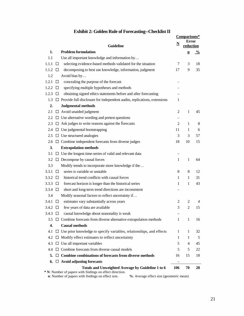
Exhibit 2 is a revised version of Armstrong, Green, and Graefe’s Table 1 (2015, p.1718). It includes 28 guidelines logically deduced from the Golden Rule. Our literature search found evidence on the effects of 19 of the guidelines. On average the use of a typical guideline reduced forecast error by 28%. Stated another way, the violation of a guideline increased forecast error by 39% on average.

We have changed the Golden Rule Checklist item on adjusting forecasts (guideline 6 in Exhibit 2) to, “Avoid adjusting forecasts.” Why? Adjusting forecasts risks introducing bias. Bias is particularly likely to occur when forecasters or clients might be subject to political pressures or to other incentives to produce a given forecast. And bias is common. For example, a survey of nine divisions within a British multinational firm found that 64% of the 45 respondents agreed that, “forecasts are frequently politically modified” (Fildes and Hastings 1994). In another study, 29 Israeli political surveys were classified according to the independence of the pollster from low to high as “in-house,” “commissioned,” or “self-supporting.” The results showed a consistent pattern: the greater the pollsters’ independence, the more accurate were their predictions. For example, 71% of the most independent polls had a relatively high level of accuracy, whereas 60% of the most dependent polls had a relatively low level of accuracy (Table 4, Shamir 1986). In addition, if one follows the primary advice in this paper to use a number of valid methods, it would be hard for experts to understand what is missing and how to adjust for that.

20

Finally, we are unable to find any evidence that adjustments would reduce forecast errors relative to the errors of forecasts derived in ways that were consistent with the guidance in the checklists presented in Exhibits 1 and 2 above. Research on adjusting forecasts from statistical models that do not combine forecasts found that, even then, adjustment typically increases errors (e.g., Belvedere and Goodwin 2017, Fildes et al. 2009) or, at best, has mixed results (e.g., Franses 2014; Lin, Goodwin, and Song 2014).

Interestingly, early research in psychology had examined the effects of subjective adjustments to forecasts. The broad conclusion was that subjective adjustments reduce forecast accuracy. Meehl (1954) used this as the basis for his primary rule for recruiting employees: If you are choosing which candidate to hire, make your decision prior to meeting the person. He illustrated adjustments with an example: “You’re in the supermarket checkout lane, piling up your purchases. You don’t say, ‘This looks like $178.50 worth to me’; you do the calculations. And once the calculations are done, you don’t say, ‘In my opinion, the groceries were a bit cheaper, so let’s reduce it by $8.00.’ You use the calculated total.” Meehl based this conclusion, on decades of research. Research since then continues to support Meehl’s law (see Grove, et al. 2000). Those who hire people, such as top executives. continue to violate this law, with sports being a major exception (teams do not like to lose).

The argument in favor of adjustments is that it may be needed when the forecasting method has not included all important knowledge and information, such as a key variable. If, however, forecasters follow the Exhibit 1 “Forecasting Methods Application Checklist” and the Exhibit 2 “Golden Rule of Forecasting Checklist” guidance— in particular on decomposition (guideline 1.1.2), including all important variables (4.3), and combining forecasts (2.5, 3.5, 4.4, 5)—there should be no important information that is not taken into account in the resulting forecast. And therefore, no need for adjustment.

Take the problem of how to forecast sales of a product that is subject to periodic promotions: a problem that is typically dealt with by judgmentally adjusting a statistical forecast of demand (see, e.g., Fildes and Goodwin 2007). The need for adjustment could be avoided by decomposing the problem into one of forecasting the level, trend, and effect of promotions separately. Expert and non-expert raters can complete the Golden Rule of Forecasting Checklist in less than an hour the first time they use it, and in much less time after becoming familiar with it. Forecasters must fully disclose their methods and clearly explain them (Guideline 1.3). To help ensure the reliability of the checklist ratings of forecasting procedures proposed or used for a forecasting problem, ask at least three people, each working independently, to do the ratings.

21

Exhibit 2: Golden Rule of Forecasting--Checklist II Comparisons*

Guideline N Error reduction

1. Problem formulation n % 1.1 Use all important knowledge and information by…

1.1.1 selecting evidence-based methods validated for the situation 7 3 18 1.1.2 decomposing to best use knowledge, information, judgment 17 9 35

1.2 Avoid bias by… 1.2.1 concealing the purpose of the forecast – 1.2.2 specifying multiple hypotheses and methods – 1.2.3 obtaining signed ethics statements before and after forecasting –

1.3 Provide full disclosure for independent audits, replications, extensions 1 2. Judgmental methods

2.1 Avoid unaided judgment 2 1 45 2.2 Use alternative wording and pretest questions – 2.3 Ask judges to write reasons against the forecasts 2 1 8 2.4 Use judgmental bootstrapping 11 1 6 2.5 Use structured analogies 3 3 57 2.6 Combine independent forecasts from diverse judges 18 10 15 3. Extrapolation methods

3.1 Use the longest time-series of valid and relevant data – 3.2 Decompose by causal forces 1 1 64 3.3 Modify trends to incorporate more knowledge if the…

3.3.1 series is variable or unstable 8 8 12 3.3.2 historical trend conflicts with causal forces 1 1 31 3.3.3 forecast horizon is longer than the historical series 1 1 43 3.3.4 short and long-term trend directions are inconsistent –

3.4 Modify seasonal factors to reflect uncertainty if… 3.4.1 estimates vary substantially across years 2 2 4 3.4.2 few years of data are available 3 2 15 3.4.3 causal knowledge about seasonality is weak –

3.5 Combine forecasts from diverse alternative extrapolation methods 1 1 16 4. Causal methods

4.1 Use prior knowledge to specify variables, relationships, and effects 1 1 32 4.2 Modify effect estimates to reflect uncertainty 1 1 5 4.3 Use all important variables 5 4 45 4.4 Combine forecasts from diverse causal models 5 5 22 5. Combine combinations of forecasts from diverse methods 16 15 18 6. Avoid adjusting forecasts –

Totals and Unweighted Average by Guideline 1 to 6 106 70 28 * N: Number of papers with findings on effect direction. n: Number of papers with findings on effect size. %: Average effect size (geometric mean)

22

SIMPLICITY IN FORECASTING: OCCAM’S RAZOR

Forecasters should use simple methods—no more complex than is needed for accuracy and usefulness. That is based on the Occam’s razor, which was proposed earlier by Aristotle. The principle has been generally accepted for centuries.

But do forecasters believe in Occam’s razor? When 21 of the world’s leading experts in econometric forecasting were asked whether more complex econometric methods yield more accurate forecasts than simple methods; 72% replied that they did. In that survey, “complexity” was defined as an index reflecting the methods used to develop the forecasting model: (1) the use of coefficients other than 0 or 1; (2) the number of variables; (3) the functional relationship; (4) the number of equations; and (5) whether the equations involve simultaneity (Armstrong 1978). The impression one gets from comparing papers on economic forecasting in leading journals from recent years with those from the 1950s is that they have been getting ever more complex.

A series of tests across different kinds of forecasting problems—such as forecasting of high school dropout rates—found that simple heuristics were routinely at least as accurate as complex forecasting methods, and often more accurate (Gigerenzer, Todd et al. 1999).

In a recent paper, we (Green and Armstrong 2015), proposed a new operational definition of simplicity, one that could be used by any client. It consisted of a 4-item checklist to rate simplicity in forecasting as the ease of understanding by a potential client. Exhibit 3 provides an abridged version of the checklist provided on ForecastingPrinciples.com. Thus, for example, it would help to use plain and simple language, only adding mathematical symbols and equations if they are needed for clarity or precision. The checklist was created before any analysis was done and it was not changed as a result of testing.

Exhibit 3: “Simple Forecasting” Checklist

Are the descriptions of the following aspects of the forecasting process sufficiently uncomplicated as to be easily understood by decision makers?

Simplicity rating

(0…10) 1. method [__] 2. representation of cumulative knowledge [__] 3. relationships in models [__] 4. relationships among models, forecasts, and decisions [__]

Simple Forecasting Average (out of 10) [___] We found 32 published papers that allowed for a comparison of the accuracy of forecasts from simple methods with those from complex methods. Four of those papers tested judgmental methods, 17 tested extrapolative methods, 8 tested causal methods, and 3 tested forecast combining methods. The findings were consistent across the methods with a range from 24% to 28%. On average across each comparison, the more complex methods had ex ante forecast errors that were 27% higher than the simpler methods. The finding was surprising because the papers the authors analyzed appeared to be proposing the more complex methods in the expectation that they would be more accurate.

23

ASSESSING FORECAST UNCERTAINTY

The uncertainty of a forecast plays a role in how one would use it. For example, if demand for

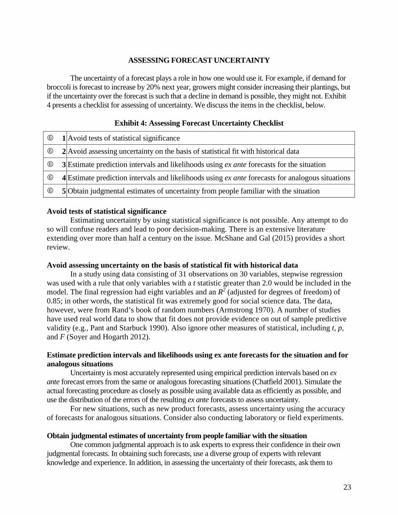
broccoli is forecast to increase by 20% next year, growers might consider increasing their plantings, but if the uncertainty over the forecast is such that a decline in demand is possible, they might not. Exhibit 4 presents a checklist for assessing of uncertainty. We discuss the items in the checklist, below.

Exhibit 4: Assessing Forecast Uncertainty Checklist

1 Avoid tests of statistical significance

2 Avoid assessing uncertainty on the basis of statistical fit with historical data

3 Estimate prediction intervals and likelihoods using ex ante forecasts for the situation

4 Estimate prediction intervals and likelihoods using ex ante forecasts for analogous situations

5 Obtain judgmental estimates of uncertainty from people familiar with the situation

Avoid tests of statistical significance Estimating uncertainty by using statistical significance is not possible. Any attempt to do

so will confuse readers and lead to poor decision-making. There is an extensive literature extending over more than half a century on the issue. McShane and Gal (2015) provides a short review. Avoid assessing uncertainty on the basis of statistical fit with historical data

In a study using data consisting of 31 observations on 30 variables, stepwise regression was used with a rule that only variables with a t statistic greater than 2.0 would be included in the model. The final regression had eight variables and an R2 (adjusted for degrees of freedom) of 0.85; in other words, the statistical fit was extremely good for social science data. The data, however, were from Rand’s book of random numbers (Armstrong 1970). A number of studies have used real world data to show that fit does not provide evidence on out of sample predictive validity (e.g., Pant and Starbuck 1990). Also ignore other measures of statistical, including t, p, and F (Soyer and Hogarth 2012). Estimate prediction intervals and likelihoods using ex ante forecasts for the situation and for analogous situations

Uncertainty is most accurately represented using empirical prediction intervals based on ex ante forecast errors from the same or analogous forecasting situations (Chatfield 2001). Simulate the actual forecasting procedure as closely as possible using available data as efficiently as possible, and use the distribution of the errors of the resulting ex ante forecasts to assess uncertainty. For new situations, such as new product forecasts, assess uncertainty using the accuracy of forecasts for analogous situations. Consider also conducting laboratory or field experiments. Obtain judgmental estimates of uncertainty from people familiar with the situation

One common judgmental approach is to ask experts to express their confidence in their own judgmental forecasts. In obtaining such forecasts, use a diverse group of experts with relevant knowledge and experience. In addition, in assessing the uncertainty of their forecasts, ask them to

24

include all sources of uncertainty and to assess their effects to the extent possible. Ask experts to write a list of all the reasons why their forecasts might be wrong. Doing so will help to moderate overconfidence (Arkes, 2001).

Experts are typically overconfident about the accuracy of their forecasts. An analysis of judgmental confidence intervals for economic forecasts from 22 economists over 11 years found the actual values fell outside the range of their 95% individual confidence intervals about 43 percent of the time (McNees 1992).

To improve the calibration of forecasters’ estimates of uncertainty, ensure that they receive timely, accurate and well summarized information on what actually happened, along with reasons why their forecasts were right or wrong. Weather forecasters use such procedures and their forecasts are well-calibrated for a few days ahead. When they say that there is a 40% chance of rain, on average over a large sample of forecasts, rain falls 40% of the time.

Estimates of the standard error of survey research, such as are provided for election polls, are typically overconfident. That is to be expected, as such estimates are based only on the uncertainty due to sampling error; they ignore response error and non-response error. These error sources are typically at least as large as the sampling error. For example, in election forecasting, the empirically estimated confidence intervals tend to be about twice as large as those used by election forecasters (Buchanan, 1986).

When uncertainty is high—such as with forecasting demand for new products—response error is also likely to be high due to survey respondents’ uncertainty about how they would make their decision (see Nisbett and Wilson 1977). Response error is likely to be the primary source of error for very new products.

Non-response error leads to large errors because the people who are most interested in the topic of the survey are much more likely to respond. This error can be reduced to some extent by the “extrapolation-across-waves” method (Armstrong and Overton 1977). Still, forecasters should consider this problem in their assessment of uncertainty. Quantitative estimates

Traditional statistical confidence intervals estimated from historical data also tend to be too narrow. One study showed that the percentage of actual values that fell outside the 95% confidence intervals for extrapolation forecasts was often greater than 50% (Makridakis, Hibon, Lusk, and Belhadjali 1987). The reason is likely to be that causal variables led to changes in the validation period.

Overconfidence arising from estimates based on the historical fit of the data to a regression model is compounded when analysts use the traditional statistics provided with regression programs. This leads them to overfit the model. The standard error of the regression is of no value to forecasters as a measure of the prediction interval (Soyer and Hogarth 2012).

As with analyses of judgmental forecasts, regression models ignore key areas of uncertainty such as the omission of key variables, the difficulty in controlling or forecasting the causal variables, inability to make accurate forecasts of the causal variables, and the difficulty of weighting the causal variables when there are intercorrelations among the causal variable. These problems are magnified when analysts strive for a close fit, and even more so when data mining techniques strive for a close fit. Such efforts reduce the likelihood the prediction intervals contain the true value. Thus, at the same time that data mining harms forecasting accuracy, it misleads clients by reporting a high level of confidence.

One way to address the problem of biases and multiple sources of error is to use a variety of different forecasting methods in the expectation that the sources of bias will vary across methods. We

25

were unable to find any testing of this proposal in the literature. However, initial small sample tests in the PollyVote project suggest that prediction intervals based on using the standard deviation of forecasts provided by six different forecasting methods were well calibrated. This seems sensible, but must be considered as speculative at this time.

Forecast errors in time series are often asymmetric, and the lack of symmetry makes estimating prediction intervals difficult. Asymmetry of errors is likely to occur when the forecasting model uses an additive trend. The most sensible procedure to deal with the problem of asymmetry is to transform the forecast and actual values to logarithms, calculate the prediction intervals using differences in the logged values, and present the results in actual values (Armstrong and Collopy 2001). The log-log transformation also makes models much easier to understand, because the coefficients represent elasticities.

Loss functions can also be asymmetric. For example, the losses due to a forecast that is too low by 50 units may differ from the losses if a forecast is too high by 50 units. But asymmetric errors are a problem for the planner, not the forecaster; the planner much assess the damages due to forecasts where the supply is too high versus those where it is too low.

METHODS LACKING PREDICTIVE VALIDITY

Those involved with demand forecasting will notice that some commonly used methods were not discussed above. This is because we were unable to find evidence that they improve accuracy relative to validated alternatives. Popular methods lacking evidence on predictive validity are listed in Exhibit 5.

Some of these methods have been tested against validated methods and have been found to be less accurate. That is the case, for example, with the Box-Jenkins method: studies of comparative accuracy have found that Box-Jenkins did poorly relative to simpler and more comprehensible alternatives (e.g. Makridakis, et al., 1984). The Box-Jenkins method is difficult for reasonably intelligent human beings to understand, thus violating Occam’s razor.

Unaided judgment

Experts’ judgment is convenient for many demand forecasting tasks, such as forecasting sales for new products, design changes, pricing, advertising, competitor behavior, or government regulations. Experts’ unaided judgments can provide useful forecasts, but only for similar, well understood, situations where they receive accurate and well-summarized feedback and where change is unlikely. Such conditions rarely apply to complex problems.

Research examining the accuracy of experts’ judgmental forecasts dates back to the early 1900s. Those findings led to the Seer-Sucker Theory (Armstrong 1980): “No matter how much evidence exists that seers do not exist, suckers will pay for the existence of seers.” The Seer-Sucker Theory has held up well over the years; in particular, a 20-year comparative evaluation study provided support (Tetlock 2005). Examples abound. Consider, for example, that many people invest in hedge funds despite the evidence that the returns from the expert stock pickers’ portfolios—especially after commissions and management fees are deducted—are inferior to those from a portfolio that mimics the stock market (Malkiel 2016).

Given the evidence to date, efforts to find better experts would be an inefficient use of resources. It would also slow the progress of scientific forecasting by keeping alive the belief that experts’ unaided judgments are useful. As we have shown above, experts are vital when their expertise is used in structured ways.

26

Focus groups

A popular method used to forecast customers’ behavior, such as demand for a proposed TV series. However, there is no evidence to support the use of this approach for demand forecasting. Furthermore, the approach violates forecasting principles. First, the participants are seldom representa-tive of the population of interest. Second, samples are small, usually less than ten. Third, in practice, questions for the participants are typically poorly structured and untested. Fourth, the responses of participants are influenced by the expressed opinions of others in the group, and by the way the moderator poses the questions. Fifth, subjectivity and bias are difficult to avoid when summarizing the responses of focus group participants. Focus groups have been used as a way to support a preferred policy by claiming that everyone had their say on the matter.

Exhibit 5: Checklist of Methods to Avoid:

Popular methods that lack predictive validity* and ignore principles

Avoided

Ignored

Method Occam’s

Razor Golden

Rule Judgmental Unaided judgment Focus groups Game theory Scenarios Quantitative Box-Jenkins / ARIMA Conjoint analysis Neural networks Data mining / Big data analytics

*Method has failed tests of ex ante forecasting accuracy relative to naïve, commonly used, and previously validated methods, or evidence of success in fair tests is not available.

Game theory Game theory involves thinking about the goals of various actors in a situation where there are

conflicts oven decisions. It involves thinking about the incentives that motivate parties and deducing the decisions they will make. The method sounds like a plausible way to forecast the decisions people will make, such as in negotiations among market participants and regulators, and in conflict situations. Authors of textbooks and research papers recommend game theory to make forecasts about outcomes of conflicts, such as how competitors would respond to a price reduction by our firm, or to an advertising campaign that compares our firm’s products to those of competitors. Our May 2017 Google Scholar search using “game theory,” “accuracy,” and “forecast” or “predict, yielded 45,000 “results.”

We have been unable to find evidence to support the claim that game theory provides useful forecasts. In the only tests of forecast validity to date, game theory experts’ forecasts of the decisions that would be made in eight real conflict situations were no more accurate than students’ unaided judgment forecasts (Green 2002 and 2005). Avoid game theory until such time as there is research that identifies conditions under which it is valid.

27

Scenarios

Scenarios are stories about the future in which the outcomes are described in detail and written in the past tense. This might be expected to help people think through the likelihood of an event. However, addition of details to the story leads people to inflate the likelihood of the event, which violates the simple logic that A plus B cannot be more likely to occur than A. In short, the expectation is that forecasts would be seriously biased (see Gregory and Duran 2001.)

Our Google Scholar search for “scenarios”, “accuracy,” and “forecast” or “predict” in May 2017 yielded 740,000 results. However, we have been unable to find any validation studies to support its value for improving accuracy. A review of research findings was unable to find any comparative studies to support the use of scenarios as a way to id forecasts of what will happen. Scenarios also violate the Golden Rule, especially because they ignore prior knowledge.

Conjoint analysis

Conjoint analysis can be used to examine how demand varies as important features of a product are varied. Potential customers are asked to make selections from a set of offers. For example, various features of a laptop computer such as price, weight, dimensions, and screen size could be varied substantially while ensuring that the variations in features do not correlate with one another. The potential customers’ choices can be analyzed by regressing them against the product features.

Conjoint analysis is based on sound principles, such as using experimental design and soliciting intentions independently from a representative sample of potential customers, so there is reason to expect the method to be useful. It is also used by practitioners. Our Google Scholar search for “conjoint analysis”, “accuracy,” and “forecast” or “predict” in May 2017 yielded over 10,000 results. However, we have been unable to find tests comparing the ex-ante accuracy of conjoint-analysis forecasts with those from other reasonable methods. Wittink and Bergestuen (2001) also failed to find such evidence. Despite the lack of sufficient testing for conjoint analysis, we believe that this method offers promise and urge that its predictive validity be tested against other methods such as experts’ judgmental forecasts—the most common practice—and judgmental bootstrapping.

Neural networks

Neural networks is a method designed to identify patterns in time-series and to use them to make forecasts. Studies on neural nets have been popular with researchers, and we found nearly 400,000 results in our May 2017 Google Scholar search for “neural networks”, “accuracy”, and “predict”, “forecast.” Little evidence on comparative forecast accuracy has been published. Perhaps the fairest and largest comparison, however, was the M3-Competition with 3,003 varied time series. In that study, neural net forecasts were 3.4% less accurate than damped trend-forecasts and 4.2% less accurate than combined extrapolations (Makridakis and Hibon 2000). The poor results are not surprising, given that neural nets ignore prior knowledge and violate Occam’s razor.

Data mining / big data analytics

Although data mining began in the 1960s with step-wise regression, we have been unable to find experimental evidence that looking for statistical patterns in data has improved ex ante forecast accuracy. In addition, data mining does not employ any of the 28 guidelines in the Golden Rule. An extensive review and reanalysis of fifty real-world data sets also found no evidence that data mining is useful (Keogh and Kasetty 2003). Finally, as noted above, data mining techniques by whatever name are expected to provide unrealistic overconfidence (narrow prediction intervals).

28

DISCUSSION

“The greatest deception men suffer is from their own opinions.” ― Leonardo da Vinci

Have the substantial improvements in knowledge on forecasting over the past half century led to more accurate forecasts in government and business? The short answer is no. Instead, forecast accuracy appears to have declined over the period. Evidence of the lack of improvement in forecasting practice and forecast accuracy, includes:

• A review of forecasting for population, economics, energy, transportation, and technology led to the conclusion that forecasting was not becoming more accurate over time Ascher (1978).

• In a review research on agriculture forecasting, Allen (1994) was unable to find evidence that forecasting practice in economics had improved over time. He then compared the accuracy of forecasts in agricultural economics from 12 studies (22 series) before 1985 and 11 studies after 1985, finding only trivial differences in accuracy.

• Based on her review of 25 years of population forecasting research, Booth (2006) found no evidence that the accuracy of population forecasts has improved over time.

• McCarthy, Davis, Golicic and Mentzer (2006) replicated two surveys on sales forecast accuracy conducted 20 years earlier, they concluded that accuracy had fallen.

• Detailed analyses of European demographic forecasts for 14 European countries concluded that accuracy improved little or not at all from the late-1970s (Keilman 2008).

However, accuracy in some areas of forecasting appears to be improving. These include

weather—up to a few days out—political elections, crime, medicine, and engineering. They have done so by adopting better forecasting procedures.

Given the evidence on their superior accuracy, why is the adoption of methods that provide more accurate forecasts so slow? For example, the benefits of combining forecasts were described in the scholarly literature more than a century ago, yet the method is seldom used.

Certainly, neglect of knowledge about the improved methods has been a barrier. Much forecasting is done by statisticians, yet a review of statistical journals found that they tend to ignore research that examines the relative advantages of different forecasting methods (Fildes and Makridakis 1995). There is no excuse for this. Relevant information on forecasting methods is published in leading journals and is summarized at ForecastingPrinciples.com, a free website.

We believe that the most common reason forecasters avoid a scientific approach to forecasting is because the decision-makers have already made a decision and are only interested in information to support that opinion. Forecasters who follow evidence-based guidelines could not be confident that their forecasts would support the clients’ preferences.

Another—and perhaps sometimes related—reason that scientific knowledge on forecasting is often overlooked, is the low priority given to it by senior managers. Forecasters and the forecasting function are given low status, and forecasters typically have had little training in forecasting methods according to surveys of forecasting practitioners. For example, a survey

29

of 81 responses from sales forecasters in electronics industry firms in Scotland found that 71% had no specific training in forecasting (Watson 1996). An earlier survey by Fildes and Hastings (1994) found 85% of forecasters lacked specific training.

Forecasting for public policy is particularly prone to the problem of decision makers who are seeking support for a decision they have already made, rather than the most accurate and relevant forecasts to guide their decision making. For example, in 1994, the first author of this paper was asked by a U.S. federal government agency to evaluate the predictions made to support the proposed adoption of “Hillary Care”. The predictions violated the Golden Rule of Forecasting by ignoring cumulative knowledge in the form of economic principles and evidence-based forecasting methods, and so the predictions amounted to nothing more than opinions. In another example, the first author was asked by a federal government agency in 2006 to join an independent panel to evaluate the “Long Run Health Care Cost Growth for the U. S. 75-year projection of the National Health expenditure as a percent of GDP.” To the distress of some panel members, the clients eventually used political guidelines rather than scientific guidelines for preparing the forecasts.

Forecasters ignore Occam’s razor by turning to ever more complex methods. They violate the Golden Rule in an effort to satisfy the clients’ need for support for their preferred policies. Clients are happy to have complex support for their policies. In this way societies still love the “rain dance.” The expected results are increased confusion and costs, higher confidence, and inaccurate forecasts.

Finally, the primary problem for this unfortunate state of affairs is that almost no one asks forecasters to provide scientific forecasts. A Solution

We believe that these trends could be reversed for those who desire accurate demand forecasts. It is an old solution and it works. Clients must tell forecasters that, as part of their contract, they must adhere to the guidelines for scientific forecasting. They could do this by providing the five checklists in this paper to the forecasters and asking that they submit completed checklists as the project develops. They would also be informed that the requirements would be audited to ensure compliance and that payment would be withheld for a failure to comply.

Those who produce forecasts that have unfortunate consequences might be sued if it can be shown that their forecasting procedures were faulty, much like the legal proceedings against medical doctors and engineers. This would apply to those who produce forecasts for public policy.

According to Tashman and Hoover (2001), many commercial forecast providers refuse to have their products reviewed. The simplest way to address this is to ask the providers what methods they use and whether they have explicit procedures for implementing the guidelines in Exhibits 2 and 3 in this paper. If concerns arise over confidentiality, the audit procedure could be conducted by an independent financial auditor. Interestingly, all of the validated methods that we discuss in this paper, except for exponential smoothing (attributed to Robert G. Brown, a consultant, who fully disclosed his method), were conceived of and developed in universities. Forecasters who go beyond the evidence-based methods available in this paper should provide evidence of predictive validity by independent testing. For an example of independent testing, consider the “Focus Forecasting”, a popular software package advertised for the accuracy of its production and inventory control forecasts. Comparisons of Focus Forecasting vs. damped-trend simple

30

exponential smoothing using five time-series of cookware demand in a production planning application found that the average errors of the smoothing forecasts were smaller, regardless of the forecast horizon or error measure used. The researchers conducted a follow up study making similar comparisons using 91 time-series from the M-Competition that led to the same conclusion (Gardner and Anderson 1997; and Gardner, Anderson-Fletcher and Wicks 2001). Our experience is that when we have required use of a checklist and made payment dependent of doing so, everyone who has accepted the task has done so effectively. This included a task involving 195 checklist items involved in assessing whether print advertisements were persuasive that was carried out by people recruited through Amazon’s Mechanical Turk.

CONCLUSIONS

Research over the past century has developed many new forecasting methods and principles. In

addition, it has revealed which forecasting methods help under given conditions, the most effective way to use each method, and the expected effects on ex ante forecast accuracy. With the exception of heavily traded financial markets, the accuracy of forecasts for most situations can be substantially improved by using simple and conservative, evidence-based forecasting methods.

We also know which methods offer little promise, and which methods harm accuracy. In particular, the “big data” movement has overlooked evidence-based methods that make the best use of available data and led forecasters to ignore prior knowledge relevant to the situation they are concerned with and to ignore the evidence-based forecasting methods we describe in this paper.

Despite much effort to help practitioners by providing understandable forecasting principles and techniques, and by making them freely available at ForecastingPrinciples.com, most firms, consultants, and software developers ignore the evidence-based methods and turn to new methods that have not been shown to improve upon current practice or persist with commonly used methods that violate forecasting principles. Sometimes these practices help forecasters to provide forecasts that support a policy favored by a client. Sometimes the failure to follow evidence-based best practice is due to ignorance of the evidence-based forecasting methods and principles. The net effect has been that, in practice, forecasting is less accurate and less intelligible than it was half a century ago.

To improve forecasting in practice, employers and clients of forecasters must require, as part of the contract, that forecasters use the five checklists for evidence-based forecasting in this paper, or improved versions. Compliance should then be assessed by having clients use these simple checklists.

Checklists are useless unless they are used. Ask and it shall be done.

REFERENCES

Key: * = contacted ** = findings confirmed by authors (applies only to substantive findings) Allen, P. G., & Fildes, R. (2001). Econometric forecasting. In J. S. Armstrong (Ed.), Principles of

Forecasting (pp. 303–362). Norwell, MA: Kluwer Academic Publishers. ** Arkes, H. R. (2001). Overconfidence in judgmental forecasting. In J. S. Armstrong (Ed.), Principles

of Forecasting (pp. 495–515). Norwell, MA: Kluwer Academic Publishers. Armstrong, J. S. (2012). Illusions in regression analysis. International Journal of Forecasting 28, 689-

694.

31

Armstrong, J. S. (2012). Predicting job performance: The Moneyball factor. Foresight: The International Journal of Applied Forecasting, 25, 31-34.

Armstrong, J. S. (2007). Significance tests harm progress in forecasting. International Journal of Forecasting, 23, 321–327.

Armstrong, J. S. (2006). Findings from evidence-based forecasting: Methods for reducing forecast error. International Journal of Forecasting, 22, 583–598.

Armstrong, J. S. (Ed.). (2001). Principles of Forecasting. Norwell, MA: Kluwer Academic Publishers. Armstrong, J. S. (2001a). Judgmental bootstrapping: Inferring experts’ rules for forecasting. In J. S.

Armstrong (Ed.), Principles of Forecasting (pp. 171–192). Norwell, MA: Kluwer Academic Publishers.

Armstrong, J. S. (2001b). Standards and practices for forecasting. In J. S. Armstrong (Ed.), Principles of Forecasting (pp. 679-732). Norwell, MA: Kluwer Academic Publishers.

Armstrong, J. S. (2001c). Combining forecasts. In J. S. Armstrong (Ed.), Principles of Forecasting (pp. 417-439). Norwell, MA: Kluwer Academic Publishers.

Armstrong, J. S. (1985). Long-Range Forecasting. New York: John Wiley and Sons. Armstrong, J. S. (1980). The seer-sucker theory: The value of experts in forecasting. Technology

Review, 83 (June/July 1980), 18-24. Armstrong, J. S. (1978). Forecasting with econometric methods: Folklore versus fact. The

Journal of Business 51, 549-64. Armstrong, J. S. (1970). How to avoid exploratory research. Journal of Advertising Research,

10, No. 4, 27-30. Armstrong, J. S., Adya, M., & Collopy, F. (2001). Rule-based forecasting: Using judgment in time-

series extrapolation. In J. S. Armstrong (Ed.), Principles of Forecasting (pp. 259–282). Norwell, MA: Kluwer Academic Publishers.

Armstrong, J. S., & Andress, J. G. (1970). Exploratory analysis of marketing data: Trees vs. regression. Journal of Marketing Research, 7, 487-492.

Armstrong, J. S., & Collopy, F. (2001). Identification of asymmetric prediction intervals through causal forces. Journal of Forecasting, 20, 273–283.

Armstrong, J. S., & Collopy, F. (1993). Causal forces: Structuring knowledge for time series extrapolation. Journal of Forecasting, 12, 103–115.

Armstrong, J. S., & Collopy, F. (1992). Error measures for generalizing about forecasting methods: empirical comparisons. International Journal of Forecasting, 8, 69–80.

Armstrong, J. S., F. Collopy, F. & Yokum, T. (2005). Decomposition by causal forces: A procedure for forecasting complex time series. International Journal of Forecasting, 21, 25-36.

Armstrong, J.S., Du, R., Green, K.C. & Graefe, A. (2016), Predictive validity of evidence-based persuasion principles, European Journal of Marketing, 50, 276-293.

Armstrong, J. S., & Graefe, A. (2011). Predicting elections from biographical information about candidates: A test of the index method. Journal of Business Research, 64, 699–706.

Armstrong, J.S., Green, K. C., & Graefe, A. (2015). Golden rule of forecasting: Be conservative. Journal of Business Research, 68, 1717–1731.

Armstrong, J. S., Morwitz, V., & Kumar, V. (2000). Sales forecasts for existing consumer products and services: Do purchase intentions contribute to accuracy? International Journal of Forecasting, 16, 383–397.

Armstrong, J. S., & Overton, T. S. (1977), Estimating nonresponse bias in mail surveys. Journal of Marketing Research 14, 396-402.

32

Armstrong, J. S., & Overton, T. S. (1971). Brief vs. comprehensive descriptions in measuring intentions to purchase. Journal of Marketing Research, 8, 114–117.

Armstrong, J.S. & Pagell, R. (2003), Reaping benefits from management research: Lessons from the forecasting principles project, Interfaces, 33, 89-111.

Batchelor, R. A., & Kwan, T. Y. (2007). Judgmental bootstrapping of technical traders in the bond market. International Journal of Forecasting, 23, 427-445.

Belvedere, V. and Goodwin. P. (2017). The influence of product involvement and emotion on short-term product demand forecasting. International Journal of Forecasting, 33, 652-661.

*Bijmolt, T.H.A., Heerde, H. J. van, & Pieters, R.G.M. (2005) New empirical generalizations on the determinants of price elasticity. Journal of Marketing Research, 42, 141-156.

Buchanan, W. (1986). Election predictions: An empirical assessment. The Public Opinion Quarterly, 50, 222-227.

Bunn, D.W. & Vassilopoulos, A.I. (1999). Comparison of seasonal estimation methods in multi-item short-term forecasting. International Journal of Forecasting, 15, 431–443.

Burgess, E. W. (1936). Protecting the public by parole and by parole prediction, Journal of Criminal Law and Criminology, 27, pp. 491–502. TBA

Chatfield, C. (2001). Prediction intervals for time series. In J. S. Armstrong (Ed.), Principles of Forecasting (pp. 475–494). Norwell, MA: Kluwer Academic Publishers.

** Collopy, F., Adya, M. & Armstrong, J. S. (2001). Expert systems for forecasting. In J. S. Armstrong (Ed.), Principles of Forecasting (pp. 285–300). Norwell, MA: Kluwer Academic Publishers.

** Collopy, F., & Armstrong, J. S. (1992). Rule-based forecasting: Development and validation of an expert systems approach to combining time-series extrapolations. Management Science, 38, 1394–1414.

Cox, J. E. & Loomis, D. G. (2001), Diffusion of forecasting principles through books. In J. S. Armstrong (Ed.), Principles of Forecasting (pp. 633-–649). Norwell, MA: Kluwer Academic Publishers.

Dawes, R. M. (1971). A case study of graduate admissions: Application of three principles of human decision making. American Psychologist, 26, 180-188.

Dillman, D. A., Smyth J. D., & Christian, L. M. (2014). Internet, Mail, and Mixed-Mode Surveys: The Tailored Design Method. (4th ed.). Hoboken, NJ: John Wiley.

Fildes, R., & Goodwin, P. (2007). Against your better judgment? How organizations can improve their use of management judgment in forecasting. Interfaces, 37, 570-576.

* Fildes, R., Goodwin, P., Lawrence, M., & Nikolopoulos, K. (2009). Effective forecasting and judgmental adjustments: an empirical evaluation and strategies for improvement in supply-chain planning. International Journal of Forecasting, 25, 3–23.

* Fildes, R. & R. Hastings (1994), The organization and improvement of market forecasting, Journal of the Operational Research Society, 45, 1-16.

* Fildes, R., & Makridakis, S. (1995). The impact of empirical accuracy studies on time series analysis and forecasting. International Statistical Review, 65, 289-308.

Franses, P. H. (2014). Expert adjustments of model forecasts: theory, practice and strategies for improvement. Cambridge, U.K.: Cambridge University Press.

Gardner, E. S., Jr. (2006). Exponential smoothing: The state of the art – Part II (with commentary). International Journal of Forecasting, 22, 637–677.

Gardner, E. S., Jr., Anderson-Fletcher, E.A., Wicks, A.G. (2001). Focus forecasting vs. exponential smoothing, International Journal of Forecasting, 17, 287-293.

33

Gardner, E. S., Jr., & Anderson, E. A. (1997). Focus forecasting reconsidered. International Journal of Forecasting, 13, 501-508.

** Gigerenzer, G. Todd, P.M.& the ABC Group (1999). Simple Heuristics That Make Us Smart. Oxford University Press.

Glueck, S., & Glueck, E. (1959). Predicting delinquency and Crime. Cambridge, MA: Harvard. Goldin, C. & Rouse, C. (2000). Orchestrating impartiality: The impact of “blind” auditions on female

musicians. American Economic Review, 90, 715-741. Goodwin, P., Dyussekeneva, K. and Meeran, S. (2013). The use of analogies in forecasting the annual

sales of new electronics products. IMA Journal of Management Mathematics, 24, 407-422. Gorr, W., Olligschlaeger, A., & Thompson, Y. (2003). Short-term forecasting of crime. International

Journal of Forecasting, 19, 579–594. ** Graefe, A. (2017). Prediction market performance in the 2016 U. S. presidential election, Foresight,

– The International Journal of Applied Forecasting, 45, 38-42. ** Graefe, A. (2015). Improving forecasts using equally weighted predictors. Journal of

Business Research, 68, 1792–1799. ** Graefe, A. (2014). Accuracy of vote expectation surveys in forecasting elections. Public

Opinion Quarterly, 78 (S1): 204–232. ** Graefe, A. (2011). Prediction market accuracy for business forecasting. In L. Vaughan-Williams

(Ed.), Prediction Markets (pp. 87–95). New York: Routledge. ** Graefe, A. and Armstrong, J.S. (2012), Forecasting elections from voters’ perceptions of

candidates' ability to handle issues, Journal of Behavioral Decision Making, DOI: 10.1002/bdm.1764.

** Graefe, A., Armstrong, J. S., Jones, R. J., & Cuzán, A. G. (2017), Assessing the 2016 U.S. Presidential Election Popular Vote Forecasts,” in The 2016 Presidential Election: The causes and consequences of an Electoral Earthquake, Lexington Books, Lanham, MD.

** Graefe, A., Armstrong, J. S., Jones, R. J., & Cuzán, A. G. (2014). Combining forecasts: An application to political elections. International Journal of Forecasting, 30, 43-54.

** Graefe, A., & Armstrong, J. S. (2011). Conditions under which index models are useful: Reply to bio-index Commentaries. Journal of Business Research, 64, 693–695.

** Graefe, A., & Armstrong, J. S. (2011). Comparing face-to-face meetings, nominal groups, Delphi and prediction markets on an estimation task, International Journal of Forecasting, 27, 183-195.

** Graefe, A., Küchenhoff, H., Stierle, V. & Riedl, B. (2015). Limitations of ensemble Bayesian model averaging for forecasting social science problems. International Journal of Forecasting, 31(3), 943-951.

Green, K. C. (2005). Game theory, simulated interaction, and unaided judgment for forecasting decisions in conflicts: Further evidence. International Journal of Forecasting, 21, 463–472.

Green, K. C. (2002). Forecasting decisions in conflict situations: a comparison of game theory, role-playing, and unaided judgment. International Journal of Forecasting, 18, 321–344.

Green, K. C., & Armstrong, J. S. (2015). Simple versus complex forecasting: The evidence. Journal of Business Research 68 (8), 1678-1685

Green, K. C., & Armstrong, J. S. (2011). Role thinking: Standing in other people’s shoes to forecast decisions in conflicts, International Journal of Forecasting, 27, 69–80.

Green, K. C., & Armstrong, J. S. (2007). Structured analogies for forecasting. International Journal of Forecasting, 23, 365–376

34

Green, K. C., Armstrong, J. S., & Graefe, A. (2015). Golden rule of forecasting rearticulated: forecast unto others as you would have them forecast unto you. Journal of Business Research, 68, 1768-1771.

Green, K. C., Armstrong, J. S., & Graefe, A. (2007). Methods to elicit forecasts from groups: Delphi and prediction markets compared. Foresight, 8, 17–20. Available from http://kestencgreen.com/green-armstrong-graefe-2007x.pdf

* Gregory, W. L., & Duran, A. (2001), Scenarios and acceptance of forecasts in In J. S. Armstrong (Ed.), Principles of Forecasting (pp. 519–540). Norwell, MA: Kluwer Academic Publishers.

Grove, W. M. et. al (2000). Clinical versus mechanical prediction: A meta-analysis, Psychological Assessment, 12, 19-30.

Hales, B. M., & Pronovost, P. J. (2006). The checklist—a tool for error management and performance improvement. Journal of Critical Care, 21, 231-235.

Hayes, S. P. Jr. (1936).The inter-relations of political attitudes: IV. Political attitudes and party regularity. The Journal of Social Psychology, 10, 503-552.

Haynes, Alex B., et al. (2009). A surgical checklist to reduce morbidity and mortality in a global population. New England Journal of Medicine, 360 (January 29), 491-499.

Hogarth, R. M. (1978). A note on aggregating opinions. Organizational Behavior and Human Performance, 21, 40-46.

** Jørgensen, M., Teigen, & Moløkken (2004). Better sure than safe? Over-confidence in judgement based software development effort prediction intervals. Journal of Systems and Software,70,79-93.

Kabat, G. C. Hyping Health Risks (2008). N.Y., N.Y.: Columbia University Press. Keilman, N. (2008). European demographic forecasts have not become more accurate during the

past 25 years, Population and Development Review 34, 137-153. * Keogh, E., & Kasetty, S. (2003). On the need for time series data mining benchmarks: A

survey and empirical demonstration. Data Mining and Knowledge Discovery, 7, 349–371.

Kim, M. S. & Hunter, J. E. (1993). Relationships among attitudes, behavioral intentions, and behavior: A meta-analysis of past research. Communication Research, 20, 331–364.

* Larrick, R. P., & Soll, J. B. (2006). Intuitions about combining opinions: Misappreciation of the averaging principle. Management Science, 52(1), 111–127.

Lin, S., Goodwin, P. and Song, H. (2014). Accuracy and bias of experts’ adjusted forecasts. Annals of Tourism Research, 48, 156-174.

Locke, E. A. (1986). Generalizing from Laboratory to Field Settings. Lexington, MA: Lexington Books.

Lovallo, D., Clarke, C., Camerer, C. (2012). Robust analogizing and the outside view: Two empirical tests of case-based decision making. Strategic Management Journal, 33, 496–512,

MacGregor, D. G. (2001). Decomposition for judgmental forecasting and estimation. In J. S. Armstrong (Ed.), Principles of Forecasting (pp. 107–123). Norwell, MA: Kluwer Academic Publishers.

Makridakis, S. G., Andersen, A., Carbone, R., Fildes, R., Hibon, M., Lewandowski, R., Newton, J. Parzen, E., & Winkler, R. (1984). The Forecasting Accuracy of Major Times Series Methods. Chichester: John Wiley.

Makridakis, S. G., Hibon, M., Lusk, E., & Belhadjali, M. (1987). Confidence intervals: An empirical investigation of time series in the M-competition. International Journal of Forecasting, 3, 489–508.

35

Makridakis, S. G. & Hibon, M. (2000). The M3-Competition: Results, conclusions and implications. International Journal of Forecasting, 16, 451–476.

Malkiel, B. G. (2016). A random walk down Wall Street: The time-tested strategy for successful investing. New York, NY: Norton.

* McCarthy, T. M., Davis, D. F., Golicic, S. L. & Mentzer, J. T. (2006). The evolution of sales forecasting management: A 20-year longitudinal study of forecasting practices. Journal of Forecasting, 25, 303–324.

McShane, B. B. & Gal, D. (2015). Blinding us to the obvious? The effect of statistical training on the evaluation of evidence. Management Science, 62, 1707-1718.

McNees, S. K. (1992), The uses and abuses of ‘consensus’ forecasts. Journal of Forecasting, 11, 703-710.

Meehl, P.E. (1954). Clinical vs. Statistical Prediction, Minneapolis: University of Minnesota Press.

Miller, D. M., & Williams, D. (2003). Miller, D. M. and Williams, D. (2003). Shrinkage estimators of time series seasonal factors and their effect on forecasting accuracy, International Journal of Forecasting, 19, 669-684.

Miller, D. M., & Williams, D. (2004). Shrinkage estimators for damping X12-ARIMA seasonals. International Journal of Forecasting, 20, 529–549.

Morwitz, V. G. (2001). Methods for forecasting from intentions data. In J. S. Armstrong (Ed.), Principles of Forecasting (pp. 33–56). Norwell, MA: Kluwer Academic Publishers.

Morwitz, V. G., Steckel, J. H., & Gupta, A. (2007). When do purchase intentions predict sales? International, Journal of Forecasting, 23, 347–364.

* Nikolopoulos, K., Litsa, A., Petropoulos, F., Bougioukos, V. & Khammash, M. (2015), Relative performance of methods for forecasting special events, Journal of Business Research, 68, 1785-1791.

Nisbett, R. E. & Wilson, T. D. (1977). Telling more than we can know: Verbal reports on mental processes, Psychological Review, 84, 231-259.

Perry, M. J. (2017). 18 spectacularly wrong predictions made around the time of first Earth Day in 1970, expect more this year. AEIdeas, April 20. Available from http://www.aei.org/publication/18-spectacularly-wrong-predictions-made-around-the-time-of-first-earth-day-in-1970-expect-more-this-year/

Rowe, G., & Wright, G. (2001). Expert opinions in forecasting role of the Delphi technique. In J. S. Armstrong (Ed.), Principles of Forecasting (pp. 125–144). Norwell, MA: Kluwer Academic Publishers.

* Shamir, J. (1986), Pre-election polls in Israel: Structural constraints on accuracy, Public Opinion Quarterly, 50, 62-75.

* Sheeran, P. (2002). Intention-behavior relations: A conceptual and empirical review. in W. Stroebe and M. Hewstone, European Review of Social Psychology, 12, 1-36.

* Soyer, E., & Hogarth, R. M. (2012). The illusion of predictability: How regression statistics mislead experts. International Journal of Forecasting, 28, 695-711.

Tashman, L. J. & Hoover, J. (2001). Diffusion of forecasting principles through software. In J. S. Armstrong (Ed.), Principles of Forecasting (pp. 651-676). Norwell, MA: Kluwer Academic Publishers.

Tellis, G. J. (2009). Generalizations about advertising effectiveness in markets. Journal of Advertising Research, 49 (2), 240-245.

36

** Tessier, T.H. & Armstrong, J.S. (2015). Decomposition of time-series by level and change. Journal of Business Research, 68, 1755–1758.

Tetlock, P. E. (2005). Expert political judgment: How good is it? How can we know? New Jersey: Princeton University Press.

Watson, M. C. (1996). Forecasting in the Scottish electronics industry. International Journal of Forecasting, 12(3), 361-371.

Wittink, D. R., & Bergestuen, T. (2001). Forecasting with conjoint analysis. In J. S. Armstrong (Ed.), Principles of Forecasting (pp. 147–167). Norwell, MA: Kluwer Academic Publishers.

Wright, M. & MacRae, M. (2007). Bias and variability in purchase intention scales. Journal of the Academy of Marketing Science, 35, 617–624.

Wright, M. & Stern, P. (2015). Forecasting new product trial with analogous series. Journal of Business Research, 68(8), 1732-1738.

Yokum, J.T. & Armstrong, J.S (1995) Beyond accuracy: Comparison of criteria used to select forecasting methods. International Journal of Forecasting, 11, 591-597.

Ziliak, S. T., & McCloskey D. N. (2004). Size matters: The standard error of regressions in the American Economic Review. The Journal of Socio-Economics, 33, 527–546.

Total Words 18,200

Text only 15,400