Demand for Money in Nepal: An ARDL

Bounds Testing Approach#

Birendra Bahadur Budha

Abstract

This paper investigates the demand for money in Nepal using the Autoregressive

Distributed Lag (ARDL) approach for the period of 1975-2011.The results based on the

bounds testing procedure reveal that there exist the cointegration among the real money

aggregates (rM1 and

rM 2 ), real income, inflation and interest rate. The real income

elasticity coefficient is found to be positive and the inflation coefficient is negative. The

interest rate coefficient is negative for both of the real monetary aggregates supporting

the theoretical explanation. In addition, the error correction models suggest that the

deviations from the long-run equilibrium are short-lived in rM1 than

rM 2 . Finally, the

CUSUM and CUSUMSQ tests reveal that the rM1 money demand function is stable, but

rM 2 money demand function is not stable implying that the monetary policy should pay

more attention to rM1 than

rM 2 .

Key words: Money Demand, Bounds text, Stability, Nepal.

JEL Classification: E410

# The earlier version of this paper is available as NRB Working Paper series, NRB-WP-12,

2012.

Assistant Director, Nepal Rastra Bank, Research Department, Central Office, Baluwatar,

Kathmandu, Nepal. Email: bcbirendra@nrb.org.np

Remarks: The views expressed in this paper are personal and do not necessarily represent the

official stance of the Nepal Rastra Bank. I would like to thank Editorial Board of NRB Economic

Review, Mr. Tulashi Prasad Ghimire, Mr. Guna Raj Bhatta and Dr. Mahesh Chaulagain for their

valuable comments.

NRB ECONOMIC REVIEW

22

I. INTRODUCTION

A stable money demand function is crucial for the conduct of monetary policy.

The stability in the function implies the stability in money multiplier and, thus,

ensures the changes in the monetary aggregates to have a specific predictable

impact on the real variables. Considering this fact, many of the studies related to

the demand for money and its stability have been conducted in developed as well

as developing countries. Accordingly, there has also been shift in the technique in

studying money demand. The partial adjustment framework and the buffer-stock

approach were mostly popular in 1980s particularly before the development of the

error correction models. The error-correction models have now become the

workhorse of the money demand research and, thus, numerous studies have been

conducted on money demand function using the cointegration technique (Sriram,

1999). In Nepal's case, few of the studies on the money demand functions, though,

have been conducted using the ordinary least squares (OLS) and the cointegration

technique developed by Johansen (1988) and Johansen and Juselius (1990), no in-

depth study of this topic has been reported yet using ARDL cointegration

technique.

Studies on the demand for money in Nepal, for instance, are by Poudel (1989),

Khatiwada (1997), Goudel (2003), Kharel and Koirala (2010) and Budha (2011).

Using the OLS method, Poudel (1989) estimated the money demand function for

Nepal with data from 1975 to 1987 and found the stable demand function for

narrow money with income elasticity coefficient being greater than unity.

Khatiwada (1997), using the OLS and stability tests like the Chow test and

CUSUM test, with Nepalese macroeconomic data from 1976 to 1996, concluded

that the demand for money in Nepal is a stable and predictable function of real

income and interest rate. The estimated income elasticity of both broad money

and narrow money in his study are more than unity. Moreover, using the

cointegration technique of Engle-Granger (1987), Khatiwada found the

cointegration among the real money balances, real income and the rate of interest.

Kharel and Koirala (2010) has employed the cointegration technique developed

by Johansen (1988) and Johansen and Juselius (1990) using the sample period of

1974/75-2009/10 and found similar result as in Khatiwada (1997) that money

demand function for both narrow and broad money is a stable and predictable

function of real income and interest rate. The disequilibrium, according to the

study, corrects more rapidly in narrow money than the broad money.

A policy regime shift, among others, is a major cause of instability in the money

demand function. Several reforms, in 1990s and since then, have been carried out

in Nepal. Some examples of the reforms are deregulation of interest rate, shift in

monetary policy stance, reforms in the capital markets, and enactment and

Demand for Money in Nepal: An ARDL Bounds Testing Approach

23

revision of the several acts and policies (Shrestha and Chowdhury, 2006). These

economic reforms have significantly changed Nepal's financial system. Against

this backdrop, the study about the stability of money demand function carries out

specific importance.

The paper aims to examine the empirical relationship between the real monetary

aggregates ( rM1 and rM 2 ), real income, inflation rate and the interest rate using the

recent econometric technique developed by Pesaran et al. (1996, 2001), known as

Autoregressive Distributed Lag (ARDL) approach to cointegration. In addition, it

attempts to determine the stability of the estimated money demand function.

The rest of the paper is organized as follows. Section II presents the model

specification. Section III presents the data and econometric methodology and

section IV discusses about the empirical results. Finally, section V presents the

conclusion.

II. MODEL SPECIFICATION

It is customary to assume that the desired level of nominal money demand

depends on the price level, a transaction (or scaling) variable and a vector of

opportunity costs (Goldfeld and Sichel, 1990), which can be written as:

.....),,()/( 21 RRYfPM …..….... (1)

Where M stands for nominal money demand, P for the price level, Y for the real

income which represents the scale variable and Ri for the elements of the vector of

the opportunity costs which possibly also includes the inflation rate. A money

demand of this type is not only the result of traditional money demand theories

but also of modern micro-founded stochastic general equilibrium model (Walsh,

2003). Following Goldfeld and Sichel (1990), the form of money demand

function employed in this paper is:

tttt

r

t RYM 3210 lnln ………. (2)

Where rM stands for real money balances i.e. (M/P), R for interest rate/ own rate

of return on money, and inflation rate- a proxy for expected inflation. µ is a

stochastic disturbance term such that t ~N (0, σ2). Based on the conventional

economic theory, the income elasticity coefficient ( 1 ) is expected to be positive

and the coefficient of the inflation ( 2 ) is expected to have negative sign. The

NRB ECONOMIC REVIEW

24

opportunity cost of holding money (i.e. inflation rate) relative to the real value of

physical assets exerts negative effects on money demand as the increase in

expected inflation lead to substitution away from money to real assets1. On the

other hand, following the literature on the speculative demand for money, the

coefficient of the interest rate, 3 is expected to have negative sign. The external

monetary and financial factors affect the money demand significantly in an open

economy through the exchange rate and expected rate of return on the money

(Lestano et al., 2009). The capital account in Nepal's balance of payments is

partially liberalized including the restrictions on portfolio investment. Capital

outflow by Nepalese residents has been completely restricted except few purposes

(Foreign Investment and Technology Transfer Act, 1992). The exchange rate and

the foreign interest rate, therefore, are not incorporated in the model assuming that

these variables have minimal impacts on the real money balances. Dekle and

Pradhan (1999) postulates that a simple linear time trend (T) can be used to

capture secular changes in the financial systems due to development of the

transaction technology. Accordingly, the linear time trend (T) is included as a

proxy for the technological change which may reflect the smooth impact of the

new financial technologies toward money demand over time.

III. DATA AND METHODOLOGY

This study is based on the annual data series from 1975 to 2011, which comprises

36 data points. Narrow money (M1) and broad money (M2) have been employed

as monetary aggregates. Narrow monetary aggregate (M1), according to the broad

monetary survey of Nepal Rastra Bank, includes the currency in circulation and

the demand deposits whereas the broad monetary aggregate (M2) includes the M1

plus the savings and call deposits and time deposits. Real monetary aggregates

( rM1 andrM 2 ) used in the study are obtained dividing the nominal monetary

aggregates by the consumer price index (CPI). The proxy for the price level (Pt) is

the consumer price index whereas the real gross domestic product (GDP) is the

proxy for the real income (Y). Similarly, the proxy for the interest rate (Rt) is the

rate of interest on the saving deposits at the commercial banks2. Due the

limitations of data, this interest rate on the saving deposits is also used in

1 Expected rate of inflation stands better for the opportunity cost of holding money where the

financial sector is not well developed as in the case of developing countries (Sriram, 1999). 2 Handa (2009) postulated that near money assets such as savings deposits in commercial banks

proved to be the closest substitutes for M1, so that their rate of return seems to be the most

appropriate variable for the cost of using M1. But, for the broad money (M2), the interest rate

on medium-term or long-term bonds would become most appropriate, since the savings

components of the broad definition of money themselves earn an interest rate close to the short

rate of interest.

Demand for Money in Nepal: An ARDL Bounds Testing Approach

25

estimating the money demand function for rM 2 . Because of the unavailability of

data on the weighted interest rate on saving deposits, the interest rate is calculated

by taking the average of minimum and maximum values of the range. The data on

these variables were taken from the various issues of the Quarterly Economic

Bulletin of Nepal Rastra Bank and Economic Survey of Ministry of Finance,

Government of Nepal.

The autoregressive distributed lag (ARDL) cointegration procedure introduced by

Pesaran and Shin (1999) and Pesaran, Shin, and Smith (1997, 2001) has been used

to examine the long-run relationship between the money demand and its

determinants. This test has several advantages over the well-known residual-based

approach proposed by Engle and Granger (1987) and the maximum likelihood-

based approach proposed by Johansen and Julius (1990) and Johansen (1992).

One of the important features of this test is that it is free from unit-root pre-testing

and can be applied regardless of whether variables are I(0) or I(1). In addition, it

does not matter whether the explanatory variables are exogenous (Pesaran and

Shin, 1997). The short-and long-run parameters with appropriate asymptotic

inferences can be obtained by applying OLS to ARDL with an appropriate lag

length. Following Pesaran et al. (1997, 2001), an ARDL representation of

equation (2) can be written as:

tttt

n

i

r

titi

n

i iti

n

i iti

n

i

r

iti

r

t

RYMR

YMM

1413121 114

1 31 21 10

lnlnlnlnln

lnlnlnln ......…… (3)

Where, Δ is the first difference operator, 0 the drift component, and t the usual

white noise residuals. The coefficients ( 41 ) represent the long-run

relationship whereas the remaining expressions with summation sign ( 41 )

represent the short-run dynamics of the model.

In order to investigate the existence of the long-run relationship among the

variables in the system, the bound tests approach developed by Pesaran et al.

(2001) has been employed. The bound test is based on the Wald or F-statistic and

follows a non-standard distribution. Under this, the null hypothesis of no

cointegration 1 = 2 = 3 = 4 =0 is tested against the alternative of cointegration

1 2 3 4 0. Pesaran et al. (2001) provide the two sets of critical values

in which lower critical bound assumes that all the variables in the ARDL model

are I(0), and the upper critical bound assumes I(1). If the calculated F-statistics is

greater than the appropriate upper bound critical values, the null hypothesis is

NRB ECONOMIC REVIEW

26

rejected implying cointegration. If such statistics is below the lower bound, the

null cannot be rejected, indicating the lack of cointegration. If, however, it lies

within the lower and upper bounds, the results is inconclusive. After establishing

the evidence of the existence of the cointegration between variables, the lag orders

of the variables are chosen by using the appropriate Akaike Information Criteria

(AIC) or Schwarz Bayesian Criteria (SBC).

The unrestricted error correction model based on the assumption made by Pesaran

et al. (2001) was also employed for the short-run dynamics of the model. Thus,

the error correction version of the ARDL model pertaining to the equation (3) can

be expressed as:

t

n

i titi

n

i iti

n

i iti

n

i

r

iti

r

t

ECR

YMM

1 14

1 31 21 10

ln

lnlnlnln ..…..… (4)

Where, is the speed of adjustment parameter and EC is the residuals that are

obtained from the estimated cointegration model of equation (3). The error

correction term (EC) is, thus, defined as: ttt

r

tt RYMEC 321 lnln .

Where, )( 121 , )( 132 , and )( 143 are the OLS estimators

obtained from equation (3). The coefficients of the lagged variables provide the

short run dynamics of the model covering the equilibrium path. The error

correction coefficient ( ) is expected to be less than zero and implies the cointegration relation. In order to check the performance of the model, the

diagnostic tests associated with the model which examines the serial correlation,

functional form and heteroscedasticity have been conducted. The CUSUM and

CUSUMSQ tests to the residuals of equation have also been applied in order to

test the model stability. The CUSUM test is based on the cumulative sum of

recursive residuals based on the first set of n observations. For the stability of the

long-run and short-run coefficients, the plot of the two statistics must stay within

the 5 % significant level.

IV. EMPIRICAL RESULTS

In order to apply the cointegration, the first step is to determine the order of

integration of each variable under study. This is because of the fact that ARDL

technique cannot be used if the order of the integration of the variables is two or

more. The Augmented Dickey Fuller (ADF) test has been employed for this

purpose both at the level and difference of the variables. The lag length used for

this test is determined using a model selection procedure based on the Schwarz

Information Criterion. The statistical results of the ADF tests are reported in table

1.

Demand for Money in Nepal: An ARDL Bounds Testing Approach

27

Table 1 shows that all the variables are stationary in the first difference. Inflation

rate is stationary at the level with constant with no trend and constant with trend.

Similarly, real money balances, both broad money ( rM 2 ) and narrow money

( rM1 ), are also trend stationary at the level. The ARDL approach to cointegration,

therefore, may be better to use since the variables are either I (0) or I (1).

Table 1. Results of ADF tests

Variables

Level First Difference

Intercept Intercept and

Trend

Intercept Intercept and

Trend rM1ln -1.20(0.66) -4.66(0.00)* -4.21(0.00)* -4.14(0.01)*

rM 2ln -1.91(0.32) -5.25(0.00)* -4.03(0.00)* -4.05(0.02)**

Yln 1.27(0.99) -2.35(0.40) -5.74(0.00)* -6.03(0.00)*

-5.35(0.00)* -5.26(0.00)* -9.67(0.00)* -9.47(0.00)*

R -1.28(0.63) -1.57(0.79) -6.13(0.00)* -6.06(0.00)* Notes: 1. * and ** denote the statistical significance at the 1% and 5% level respectively.

2. The numbers within the parentheses for the ADF statistics are the p-values.

In the first stage of ARDL procedure, we impose arbitrary and the same number

of lags on each first differenced variables in equation (3) and carry out F-test. The

result will depend on the choice of the lag length (Bahmani-Oskooee & Brooks,

2007). Akaike's and Schwarz's Baysian Information Criteria have been employed

in order to select the optimal lag length. The LM test has been used in order to test

the serial correlation in residuals.

Table 2. Statistics for Selecting Lag Order

Narrow Money, rM1 Broad Money,

rM 2

Lags AIC SBC LM(1) AIC SBC LM(1)

1 -3.36 -2.78 0.59** -3.64 -3.06 0.27**

2 -3.16 -2.40 0.66** -3.40 -2.64 4.18*

3 -3.56 -2.61 0.51** -3.50 -2.55 0.01**

Note: * and ** refers to marginal significance level at 1% and 10% respectively.

The results for selecting lag order are reported in table 2. The results of both AIC

and SBC criteria are similar for the model of broad money. For the model of

narrow money, AIC and SBC criteria give the conflicting results. Taking lag of

one or three in the model of narrow money does not make any significant

difference in the value of F-statistic so the optimal lag length selected and

reported for the ARDL equation (3) with no serial correlation problem is one for

both rM1 and rM 2 .

NRB ECONOMIC REVIEW

28

The existence of the long-run relationship between money demand and its

components has been tested by calculating F-statistics with one lag. The F-

statistics is calculated by applying Wald tests that impose zero value restriction to

only one period lagged level coefficient value of the variables. These test results

are reported in table 3 with new critical values as suggested by Pesaran et al.

(2001) and Narayan (2004) for bounds test procedure.

Table 3. Bounds tests for Cointegration Analysis

Order of Lag 1 rM1 6.70*

rM 2 5.86*

Notes:

1. The relevant critical value bounds are obtained from Table C1. iv (with an unrestricted

intercept and restricted trend; with three regressors k=3) in Pesaran et al. (2001). These are

2.97- 3.74 at 90 %, 3.38-4.23 at 95% and 4.30-5.23 at 99%.

2. * denotes the significance at 99%.

3. The critical values presented in Pesaran et al. (2001) are based on large samples (Narayan,

2004). For small sample sizes ranging from 30 to 80 observations, Narayan (2004) provides a

set of critical values, which are 2.496-3.346 at 90%, 2.962-3.910 at 95% and 4.068-5.250 at

99%.

The computed F-statistics in table 3 was compared with the critical values

provided by Narayan (2004) for small samples. The results clearly indicate that,

since computed F-statistic is greater than critical values, there exists cointegration

between real money balances, real income, inflation rate and interest rate.

The lag length for each variable need not be identical except for the identification

purpose above3. In this stage, a more parsimonious model is selected for the long-

run money demand using the Akaike information criteria. Pesaran and Shin

(1997) and Narayan (2004) suggested two as the maximum order of lags in the

ARDL approach for the annual data series. The total number of regressions to be

estimated for the ARDL (p, q, r, s) is (p+1)k , where p is the maximum number of

lag order to be used and k is the number of variables in the equation. As p=2 and

k=4, the total number of regressions to be estimated are 81. For this procedure,

the Microfit 5.0 software program has been used and, thus, estimated ARDL (1, 0,

0, 0) model for the narrow money and ARDL (2, 0, 1, 0) model for broad money

based on AIC criterion.

The long-run coefficients of the real money balances ( rM1 and rM 2 ) are reported in

table 4 and 5. The table 4 shows that the coefficients of real income, inflation rate

and interest rate all have the expected sign as suggested by economic theories, but

3 See Pesaran (2001) and Dagher and Kovanen (2011).

Demand for Money in Nepal: An ARDL Bounds Testing Approach

29

these are statistically insignificant. The long run model of the corresponding

ARDL (1, 0, 0, 0) for narrow money ( rM1 ) can be written as:

tRYM tt

r 04.0009.0003.0ln42.020.0ln 1 ………(5)

In table 5, the estimated long-run coefficients for broad money demand are

presented. The coefficients of real income, although statistically insignificant,

have the expected positive sign indicating the positive relationship between real

income and money demand. The coefficient of the inflation rate is negative

supporting the theoretical explanation. This implies that people prefer to substitute

real assets for money balances. Similarly, the coefficient of the interest rate is

negative and statistically insignificant. The long-run model of the corresponding

ARDL (2, 0, 1, 0) for broad money ( rM 2 ) is:

tRYM tt

r 08.0004.0003.0ln06.091.4ln 2 ……..……..(6)

Table 4. Estimated Long-run Coefficients of Real Money Balances

Dependent Variable: Narrow Money Aggregate, rM1ln

Coefficient S.E t-Statistic p-value

Yln 0.42 0.33 1.29 0.21

-0.003 0.005 -0.64 0.53

R -0.009 0.01 -0.77 0.45

Constant 0.20 3.91 0.05 0.96

Trend 0.04* 0.02 2.69 0.01 Note: * denotes the significance at 99%.

Table 5. Estimated Long-run Coefficients of Real Money Balances

Dependent Variable: Broad Money Aggregate, rM 2ln

Regressor Coefficient S.E t-Statistic p-value

Yln 0.06 0.21 0.30 0.29

-0.003 0.004 -0.81 0.43

R -0.004 0.008 -0.50 0.62

Constant 4.91* 2.54 1.94 0.06

Trend 0.08** 0.01 7.48 0.00 Note: * and ** denote the significance at 99% and 90% respectively.

The short-term dynamics of the model has been examined by estimating an error

correction model in equation (4). In the short run, the deviations from the long-run

equilibrium can occur because of the shocks in any of the variables in the model.

The diagnostic tests, which are used in this paper to examine the properties of the

NRB ECONOMIC REVIEW

30

model, include the test of serial autocorrelation (χ2Auto), normality (χ2Norm),

heteroskedasticity (χ2BP) and omitted variables /functional form (χ2RESET). The

results of the short-run dynamic money demand models and the associated

diagnostic tests are reported in table 6 and 7.

Table 6 shows that the estimated lagged error correction term (ECM-1) is negative

and statistically significant. This result indicates the cointegration among the

variables: narrow money, real income, inflation and interest rate. The absolute

value of the coefficient of error correction term (i.e. 0.81) implies that about 81

percent of the disequilibrium in the real money demand is adjusted toward

equilibrium annually. For instance, if the real money demand ( rM1 ) exceeds its

long-run relationship with the other variables in the model, then the money

demand adjust downwards at a rate of 81% per year. As presented in the table 6,

there is no evidence of diagnostic problem with the model. The Lagrange

Multiplier (LM) test of serial correlation indicates the evidence of no serial

correlation since the estimated LM value or χ2Auto is less than the critical values.

The Jarque-Bera normality test implies that the residuals are normally distributed.

The Breusch-Pagan test (BP) for heteroscedasticity shows that the disturbance

term in the model is homoscedastic. The Ramsey's RESET test for functional

specification shows that the calculated RESET statistic or χ2RESET is less than its

critical values and, thus, the ARDL model is correctly specified.

Table 6. Error Correction Representation of ARDL Model, ARDL (1, 0, 0, 0)

Dependent Variable: Narrow Money, rM1ln

Regressor Coefficient t-statistic p-value rM 1,1ln 0.24*** 1.70 0.09

Yln 0.31 1.48 0.15

Δπ -0.004** -0.66 0.03

ΔR -0.005 -0.66 0.52

Ecm-1 -0.81* -5.82 0.00

Constant 0.17* 6.89 0.00

Trend 0.03* 5.63 0.00

R2= 0.63 R

2adj= 0.55 F = 7.92 (0.00) S.E. = 0.04 DW= 1.88

AIC=-3.47

Diagnostic test:

A. Serial correlation χ2Auto (2)=0.55 (0.76)

B. Functional Form χ2

RESET (2)=0.22(0.80)

C. Normality χ2Norm = 0.01(0.99)

D. Heteroscedasticity χ2BP (2) =5.96(0.47)

Notes: 1. *, ** and *** indicate the significance at the 99%, 95% and 90% level respectively.

2. The value in parentheses are the probabilities

Demand for Money in Nepal: An ARDL Bounds Testing Approach

31

Table 7. Error Correction Representation of ARDL Model, ARDL (2, 0, 1, 0)

Dependent Variable: Broad Money, rM 2ln

Regressor Coefficient t-statistic p-value rM 1,2ln 0.17 1.06 0.30

rM 2,2ln -0.09 -0.63 0.54

Yln 0.22 1.12 0.27

Δπ -0.004** -2.45 0.02

Δπ-1 -0.0003 -0.02 0.98

ΔR -0.001 -0.15 0.87

Ecm-1 -0.68* -5.97 0.00

Constant 0.16* 5.01 0.00

Trend 0.02* 3.11 0.00

R2= 0.55 R

2adj= 0.40 F = 3.77 (0.01) S.E. = 0.03 DW= 1.85

SBC=-3.66

Diagnostic test:

A. Serial correlation χ2Auto (2)=0.45 (0.79)

B. Functional Form χ2

RESET (2)=0.42(0.66)

C. Normality χ2Norm = 0.01(0.99)

D. Heteroskedasticity χ2

BP (2)=8.07(0.42) Notes: 1. ** indicates the significance at the 99% level.

2. The value in parentheses are the probabilities.

Table 7 presents the results for broad monetary aggregate, rM 2 . The coefficient of

the error correction term is negative and statistically significant, indicating the

evidence of the cointegration among the broad money and other variables in the

model. The high value of the error correction term for M2 implies relatively faster

adjustment in money demand when shocks arise. The coefficient of error

correction term (i.e. 0.68) implies that about 68 % of total adjustment takes

annually when shock arises. The smaller error correction coefficient of rM 2 than rM1 implies the slow speed of adjustment when shocks arises. This result is

consistent with the previous study by Kharel and Koirala (2010). The diagnostic

tests applied to the error correction model indicate that there is no evidence of

serial correlation and heterosketasticity. In addition, the RESET test implies the

correctly specified ARDL model and the Jarque-Bera normality test indicates that

the residuals are normally distributed.

In the final stage, the stability of the long-run coefficients is examined by using

the CUSUM and CUSUM squares tests. The graphical presentation of these tests

is presented in the figure below.

NRB ECONOMIC REVIEW

32

-16

-12

-8

-4

0

4

8

12

16

84 86 88 90 92 94 96 98 00 02 04 06 08 10

CUSUM 5% Significance

Figure 1: Cumulative Sum of Recursive Residuals(M1)

-0.4

-0.2

0.0

0.2

0.4

0.6

0.8

1.0

1.2

1.4

84 86 88 90 92 94 96 98 00 02 04 06 08 10

CUSUM of Squares 5% Significance

Figure 2: Cumulative Sum of Squares of Recursive Residuals(M1)

-15

-10

-5

0

5

10

15

88 90 92 94 96 98 00 02 04 06 08 10

CUSUM 5% Significance

Figure 3: Cumulative Sum of Recursive Residuals (M2)

-0.4

-0.2

0.0

0.2

0.4

0.6

0.8

1.0

1.2

1.4

88 90 92 94 96 98 00 02 04 06 08 10

CUSUM of Squares 5% Significance

Figure 4: Cumulative Sum of Squares of Recursive Residuals (M2)

Since the plots of CUSUM and CUSUMSQ statistic for rM1 are within the critical

lines at the 5% significance level, the money demand functions for rM1 is stable.

The plot of CUSUM, though, is within the critical lines at the 5% significance

level, the plot of CUSUMSQ does not lie within the critical limits implying some

instability in the money demand function for rM 2 . Since the plot of CUSUMSQ

for rM 2 is returning back towards the critical bands, the deviation is only

transitory. The central bank, since the money demand function for narrow money

is relatively stable than broad money, should pay more attention to rM1 for the

monetary policy purposes.

Demand for Money in Nepal: An ARDL Bounds Testing Approach

33

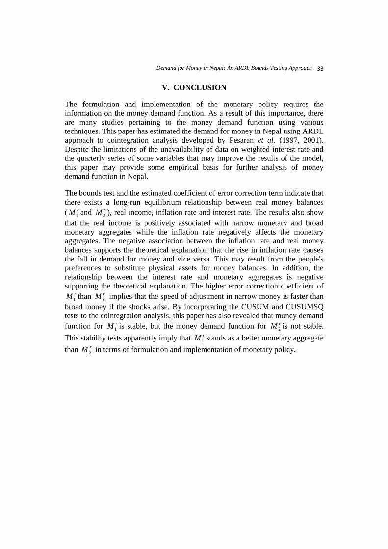
V. CONCLUSION

The formulation and implementation of the monetary policy requires the

information on the money demand function. As a result of this importance, there

are many studies pertaining to the money demand function using various

techniques. This paper has estimated the demand for money in Nepal using ARDL

approach to cointegration analysis developed by Pesaran et al. (1997, 2001).

Despite the limitations of the unavailability of data on weighted interest rate and

the quarterly series of some variables that may improve the results of the model,

this paper may provide some empirical basis for further analysis of money

demand function in Nepal.

The bounds test and the estimated coefficient of error correction term indicate that

there exists a long-run equilibrium relationship between real money balances

( rM1 and rM 2 ), real income, inflation rate and interest rate. The results also show

that the real income is positively associated with narrow monetary and broad

monetary aggregates while the inflation rate negatively affects the monetary

aggregates. The negative association between the inflation rate and real money

balances supports the theoretical explanation that the rise in inflation rate causes

the fall in demand for money and vice versa. This may result from the people's

preferences to substitute physical assets for money balances. In addition, the

relationship between the interest rate and monetary aggregates is negative

supporting the theoretical explanation. The higher error correction coefficient of rM1 than rM 2 implies that the speed of adjustment in narrow money is faster than

broad money if the shocks arise. By incorporating the CUSUM and CUSUMSQ

tests to the cointegration analysis, this paper has also revealed that money demand

function for rM1 is stable, but the money demand function for rM 2 is not stable.

This stability tests apparently imply that rM1 stands as a better monetary aggregate

than rM 2 in terms of formulation and implementation of monetary policy.

NRB ECONOMIC REVIEW

34

REFERENCES

Abdullah, H., Ali, J. & Matahir, H. 2010. "Re-Examining the Demand for Money in Asean-5

Countries." Asian Social Science. Vol. 6, No 7.

Achsani, N.A. 2010. "Stability of Money Demand in an Emerging Market Economy: An Error

Correction and ARDL Model for Indonesia." Research Journal of International Studies-Issue

13, 2010.

Adhikary, D.K., Pant, R. & Dhungana, B.R. 2007. "Study on Financial Sector Reform in Nepal."

SANEI, Pakistan Institute of Development Economics, Quaid-i-Azam University, Islamabad,

Pakistan.

Azim, P., Ahmed, N., Ullah, S., Zaman, B. & Zakaria, M. 2010. "Demand for Money in Pakistan:

an ARDL Approach." Global Journal of Management and Business Research. Vol. 10, Issue

9.

Bahmani-Oskooee, M. & Wang, Y. 2007. "How Stable is the Demand for Money in China?"

Journal of Economic Development. Vol 32, 2007.

Banaian, K. and Ratha, A. 2008. "Stability of the Euro-Demand Function." Economics Faculty

Working Papers. St. Cloud State University, USA.

Brissimis, S.N., Hondroyiannis, G., Swamy, P.A.V.B & Tavlas, G.S. 2003. "Empirical Modelling

of Money Demand in Periods of Structural Change: The Case of Greece." Working Paper No

1, Bank of Greece, Greece.

Budha, B.B. 2011. "An Empirical Analysis of Money Demand Function in Nepal." Economic

Review, Occasional Paper, No 23. Nepal Rastra Bank, Nepal.

Dagher, J. & Kovanen, A. 2011. "On the Stability of Money Demand in Ghana: A Bounds Testing

Approach." IMF Working Paper-WP/11/273. International Monetary Fund, Washington,

USA.

Delke, R. & Pradhan, M. 1999. "Financial Liberalization and Money Demand in the ASEAN

countries." International Journal of Finance and Economics, 4.

Dharmaratne, W.R.A. 2009. Demand for Money in Sri Lanka During the Post Liberalization

Period. Staff Studies-Vol. 34, N0 1&2. Central Bank of Sri Lanka, Colombo, Sri Lanka.

Dritsakis, N. 2011. "Demand for Money in Hungary: An ARDL Approach." Review of Economics

and Finance. Available at http://users.uom.gr/~drits/publications/ARDL.pdf.

Duca, J.V. & VanHoose, D.D. 2004. "Recent developments in understanding the demand for

money." Journal of Economics and Business, 52.

Engle, R.F., & Granger, C.W.J. 1987. "Co-Integration and Error Correction: Representation,

Estimation, and Testing." Econometrica, Vol.55, No 2.

Goldfeld, S.M. & Sichel, D.E. 1990. The Demand for Money. in B.M. Friedman and F.H. Hahn,

eds. Handbook of Monetary Economics, Elsevier, Amsterdam, Netherlands.

Handa, J. 2009. Monetary Economics. Second Edition. New York: Routledge, Taylor & Francis

Group, USA.

Demand for Money in Nepal: An ARDL Bounds Testing Approach

35

Hill, C. R., Griffiths, W.E. & Lim, G. 2011. Principles of Econometrics. Fourth Edition. John

Wiley & Sons, Inc., USA.

Johansen, S. & Juselius, K. 1990. "Maximum Likelihood Estimation and Inference on

Cointegration with Application to the Demand for Money." Oxford Bulletin of Economics and

Statistics, 52.

Johansen, S. 1988. "Statistical Analysis of Cointegrating Vectors." Journal of Economic Dynamics

and Control, Vol. 12, No. 2/3.

Khan, M.A. & Sajjid, M.J. 2005. "The Exchange Rates and Monetary Dynamics in Pakistan: An

Autoregressive Distributed Lag (ARDL) Approach." The Lahore Journal of Economics.

Available at http://mpra.ub.uni-muenchen.de/6752/

Kharel, R.S. & Koirala, T.P. 2010. "Modeling Demand for Money in Nepal." NRB Working Paper,

NRB/WP/6. Nepal Rastra Bank, Nepal.

Khatiwada, Y.R. 1997. "Estimating the Demand for Money in Nepal: Some Empirical Issues".

Economic Review, Occasional Paper NRB/WP-9, Nepal Rastra Bank, Nepal.

Lestano, Jacobs, J.P.A.M. & Kuoer, G.H. 2009. "Broad and Narrow Money Demand and Financial

Liberalization in Indonesia, 1980Q1-2004Q4." Working Paper. University of Groningen,

Netherlands.

Lutkepohl, H. & Kratzig, M. 2004. Applied Time Series Econometrics. Cambridge University

Press, Cambridge, UK.

MOF. 2011. Economic Survey. Ministry of Finance, Government of Nepal, Kathmandu, Nepal.

MOF. 2012. Economic Survey. Ministry of Finance, Government of Nepal, Kathmandu, Nepal.

Narayan, P.K. & Narayan, S. 2008. "Estimating the Demand for Money in an Unstable Open

Economy: The Case of the Fiji Islands." Economic Issues, Vol. 13, Part 1, 2008.

Narayan, P.K. 2004. "Reformulating Critical Vlues for the Bounds F-statistics Approach to

Cointegration: An Application to the Tourism Demand Model for Fiji." Discussion Papers,

ISSN 1441-5429. Department of Economics, Monash University, Victoria, Australia.

NRB. Quarterly Economic Bulletin (Various Issues). Vol. 46, No. 43. Nepal Rastra Bank, Nepal.

Omotor, D.G. & Omotor, P.E. 2011. Structural Breaks, Demand for Money and Monetary Policy

in Nigeria. Available at http://www.csae.ox.ac.uk/conferences/2011-EDiA/papers/291-

Omotor.pdf .

Pesaran, M. H. & Shin, Y. 1997. "Autoregressive Distributed Modeling Approach to Cointegration

Analysis." Available at http://www.eprg.org.uk/faculty/pesaran/ardl.pdf.

Pesaran, M.H., Shin, Y. & Smith, R.J. 1999. "Bounds Testing Approaches to the Analysis of Long

Run Relationships." Available at http://www.econ.cam.ac.uk/ faculty/pesaran/pss1.pdf

Pesaran, M. H. & Shin, Y. 2001. "Bounds Testing Approaches to the Analysis of Level

Relationships." Journal of Applied Econometrics, 2001, 16.

Poudyal, S.R. 1989. "The Demand for Money in Nepal." Economic Review, Occassional Paper,

NRB/W-3. Nepal Rastra Bank, Nepal.

NRB ECONOMIC REVIEW

36

Renani, H. 2007. "Demand for Money in Iran: An ARDL approach." MPRA Paper No. 8224.

Available at http://mpra.ub.uni-muenchen.de/8224/.

Shrestha, M. B. & Chowdhury, K. 2006. "Financial Liberalization Index for Nepal." International

Journal of Applied Econometrics and Quantitative Studies, Vol. 3-1.

Sriram, S.S. 1999. "Survey of Literature on Demand for Money: Theoretical and Empirical Work

with Special Reference to Error-Correction Models." IMF Staff Paper, WP/99/64.

Washington: International Monetary Fund, USA.

Sriram, S.S. 2001. 'A Survey of Recent Empirical Money Demand Studies." IMF Staff Papers,

Vol. 47, No 3. Washington: International Monetary Fund, USA.

Walsh, C. E. 2003. Monetary Theory and Policy. Second Edition. The MIT Press, USA.