Demand Estimation with Strategic Complementarities:Sanitation in Bangladesh

Raymond GuiterasNCSU

James LevinsohnYale University

Ahmed Mushfiq MobarakYale University

January 11, 2019

Abstract

For many products, the utility of adoption depends on the share of other house-holds that adopt. We estimate a structural model of demand that allows for theseinter-dependencies. We apply our model to the adoption of household latrines – atechnology that has large consequences for public health. We estimate the model usingdata from a large-scale experiment covering over 18,000 households in 380 communi-ties in rural Bangladesh, where we randomly assigned incentives to purchase latrines.Subsidies were randomly assigned at the household level to identify the direct effectof price, and subsidy saturation was randomly varied at the community level to iden-tify strategic complementarities in demand. We conduct counter-factual simulations toanalyze the policymaker’s tradeoffs along price, saturation and scope margins: To raiseaggregate latrine adoption, is it better to intensely subsidize a few, or widely dispersesubsidies across households or communities? We also analyze the effects of targetingsubsidies on the basis of household poverty, social position, or neighborhood popula-tion density. Finally, we use additional experiments to explore mechanisms underlyingthe complementarity in demand, and find that shame and changing social norms aredriving factors.

Email: rpguiter@ncsu.edu, james.levinsohn@yale.edu, ahmed.mobarak@yale.edu. For helpful comments wethank Francesco Amodio, Steve Berry, Gilles Duranton, John Hoddinott, Ganesh Iyer, Laura Lasio, MollyLipscomb, Duncan Thomas, Denni Tomassi, Sandeep Sukhtankar, Adrian Tschoegl, seminar participantsat Columbia, Harvard/MIT, McGill, North Carolina State University, UC-San Diego, University of CapeTown, University of Vienna, University of Washington, Wharton, Yale SOM, Yale Political Science, BIDS(Dhaka) and conference participants at the New Frontiers in Development Economics Conference at UConn,GGKP Annual Conference (World Bank/OECD/U.N.), NEUDC 2018, Southern Economic Association 2018,Y-RISE Spillovers Conference 2018, and the China India Customer Insights Conference at the Cheung KongGSB. We thank Meir Brooks, Julia Brown, Zhi Chen, Seungmin Lee, Benjamin Lidofsky, Matthew Krupoff,Derek Wolfson, Tetyana Zelenska and Hangcheng Zhao for outstanding research assistance, Innovations forPoverty Action-Bangladesh (Mahreen Khan, Ishita Ahmed, Ariadna Vargas, Rifaiyat Mahbub, Mehrab Ali,Mehrab Bakhtiar, Alamgir Kabir, Ashraful Haque) for field support, the Bill and Melinda Gates Foundationand the International Growth Centre for financial support, and Wateraid-Bangladesh and VERC for theirpartnership in implementing the interventions. Mobarak acknowledges support from a Carnegie FellowshipGrant ID G-F-17-54329.

1 Introduction

The utility of a purchase often depends on the number or share of others making the same

purchase. This phenomenon has many labels – “peer effect,” a “network externality,” or a

“strategic complementarity in demand” – and there are myriad examples. Strategic com-

plementarity in demand exists when farmers learn from their neighbors and decide whether

to adopt a new technology (Conley and Udry 2010). It is present when a consumer decides

whether to adopt mobile phone service, and the value of the service depends on how many

others are on the same network (Bjorkegren 2018). Economists have identified demand com-

plementarities in decisions about energy conservation (Allcott 2011), how much labor effort

to expend (Mas and Moretti 2009), whether to migrate (Munshi 2003; Meghir et al. 2015;

Akram et al. 2017), purchase insurance (Kinnan 2017), or enter the labor force in the pre-

sence of gender norms on who works (Iversen and Rosenbluth 2010; Bertrand 2011). This

list is illustrative, but hardly exhaustive.

When strategic complementarities are positive, as in all the examples listed above, a policy to

promote adoption may be welfare enhancing. In many instances, the key barrier to adoption

is price (J-PAL 2011), which makes subsidies an obvious policy lever. However, the precise

design of subsidy policy in the presence of strategic complementarities is not straightforward.

There are two main challenges – one conceptual and one econometric.

The conceptual challenge relates to understanding the effects subsidies will have in the

presence of interdependent decision-making. While subsidies have the usual direct effect of

increasing demand by reducing price, they also may have an indirect spillover effect on others’

adoption decisions. We model this formally below by introducing a strategic complementarity

into the household adoption decision. This interdependence in decision-making introduces

complexities into the prospective analysis of subsidy policy. For example, if our goal is to

maximize adoption, should a fixed subsidy budget be widely distributed, or should a smaller

number of households be targeted with larger subsidies? When household heterogeneity

1

is modeled, what type of targeting is most efficacious? Indeed, even computing the price

elasticity of demand, a key primitive to any analysis, is not straightforward when prices

affect a household’s decision both directly and through the decisions of its peers.

The second challenge to fashioning subsidy policy is econometric and is often referred to as

“The Reflection Problem” (Manski 1993).

“[The Reflection Problem] arises when a researcher observing the distribution of

behaviour in a population tries to infer whether the average behaviour in some

group influences the behaviour of the individuals that comprise that group.”

Manski concluded his influential paper by noting that “Given that identification based on

observed behaviour alone is so tenuous, experimental and subjective data will have to play

an important role in future efforts to learn about social effects.” We address the econometric

challenge by taking Manski’s advice to heart and collecting experimental data. We estimate

key demand parameters of a model of inter-dependent decision-making using a randomized

controlled trial (RCT) that was designed to identify both the direct effect of prices and the

spillover effect via interdependent demand (Manski’s “social effect”).

While these challenges of evaluating subsidy policy in the presence of strategic complemen-

tarities are present in many contexts, our specific empirical application is the adoption of

latrines in a developing country. This is an important policy issue in its own right, for sa-

nitation practices have significant consequences for human health and welfare. About one

billion people practice open defecation (OD) (WHO and UNICEF 2014). The attendant

health burden falls principally on the poor. Diarrheal disease kills nearly one million people

per year (Pruss-Ustun et al. 2014), and is the cause of nearly 20% of deaths of children un-

der five in low income countries (Mara et al. 2010). Latrine use has been shown to improve

public health and generate positive externalities (Spears 2012; Pickering et al. 2015; Hathi

et al. 2017; Geruso and Spears 2018; Gautam 2017), but adoption rates remain low. Price is

a key determinant of latrine adoption, making subsidies an important policy lever (Guiteras

2

et al. 2015; Cameron and Shah 2019; Gautam 2018).

Strategic complementarities are likely important in the sanitation adoption decision for at

least three reasons. First is an epidemiological or technical complementarity. The health

improvements a household experiences from adoption may be larger if neighboring households

also adopt, while the health benefits of adoption are muted or nullified if neighbors continue

to practice OD.1 Second, social norms may be important. In a community in which OD is

the norm, the “social cost” or shame associated with practicing OD may be absent, whereas

it may be very high in a community in the social norm is to use a toilet (Pattanayak et al.

2009). Third, investing in latrines may allow neighbors to learn about the technology and

change their perceptions about the net benefits of adoption.

We conducted a large-scale field experiment on sanitation behavior with over 18,000 hou-

seholds in 380 communities in rural Bangladesh. We randomly varied (1) the price specific

households faced to identify the direct effect of price on adoption, and (2) subsidy “satura-

tion” – the fraction of each community offered subsidies – to identify the indirect effect of

others’ adoption decisions.2 We then estimate a discrete choice model of demand in the pre-

sence of strategic complementarities. Both the large number of communities, and the large

number of households per community in our experiment are useful for precisely estimating

the own price and the demand spillover effects. The estimated structural model then allows

us to evaluate several prospective policies.

Our estimates indicate that subsidies encourage latrine adoption, and that adoption decisions

are strategic complements. Holding own price constant, a household becomes more likely to

invest if a larger fraction of its community are also offered a subsidy. These estimates form

the basis for our counterfactual simulations to identify subsidy policies that would increase

1A latrine may only generate a return in the household’s health production function once the surroundingenvironment becomes sufficiently clean. In the multi-country study with health outcomes data, (Gertler etal. 2015) argues that communities need to reach a threshold in sanitation coverage before we see impacts onchild height.

2Other RCTs that randomly vary program saturation include Crepon et al. (2013), Akram et al. (2017),Deutschmann et al. (2018) and Cai and Szeidl (2018).

3

aggregate adoption rates in a community. We explore the effects of widely distributing the

subsidy budget versus concentrating larger subsidies to a few; targeting subsidies on the

basis of household characteristics such as poverty or social network position; and targeting

on the basis of community attributes such as population density. These simulations help us

design mechanisms that increase aggregate adoption without changing the subsidy budget

outlay.

We included additional randomized experiments to identify behavioral mechanisms that may

underlie the strategic complementarity in demand. We find that social norms are relevant,

but not in the way that we had expected. Subsidizing socially marginal households to invest

in latrines produces a positive spillover on others’ adoption, whereas adoption by community

leaders and socially central households do not influence others as much. We interpret this to

mean that shame is a key driver of behavior in this setting. When people occupying lower

social strata start using a new latrine technology, it becomes shameful for others to continue

defecating in the open. Changes in social norms appear to be more “downward-facing”

rather than “upward-looking.” This insight is useful for the design of social marketing of new

products, behaviors, and technologies in sociology (Kim et al. 2015), economics (BenYishay

and Mobarak 2018; Akbarpour et al. 2018; Banerjee et al. 2013; Beaman et al. 2018) and

marketing (Chan and Misra 1990). Leadership and centrality are popular concepts in these

applications, but our results suggest that social influence may work very differently in some

settings.

Our analysis demonstrates how two methodologies that are often viewed as competing alter-

natives – RCTs and structural estimation – can fruitfully serve as complements. We design

our RCT to convincingly identify the two key parameters needed for our model (associated

with price and complementarity). However, given the recursive nature of direct and higher

order indirect effects when strategic complementarities are present, the RCT estimates alone

are not sufficient to analyze the marginal effect of a price change. We follow in the footsteps

4

of others who have fruitfully combined these approaches (Todd and Wolpin 2006; Kremer et

al. 2011; Duflo et al. 2012; Attanasio et al. 2012).

The methodology developed and implemented in this paper is applicable to contexts beyond

sanitation. Our general approach is relevant to conducting policy analysis whenever demand

inter-linkages are present. As noted at the outset, strategic complementarities are present

across many fields of economics and their prevalence extends to a broad spectrum of the

social sciences. For example, social norms even guide the willingness to engage in bullying

(Paluck et al. 2016) or in militia violence and genocide (Yanagizawa-Drott 2014). They can

affect decisions on how much to contribute to public goods or charity (Kessler 2013), whether

to purchase health products (Oster and Thornton 2012; Kremer and Miguel 2007), or the

type of financial asset chosen (Bursztyn et al. 2014). The effectiveness of policies to either

promote or deter such behaviors and actions depend on the nature or size of the behavioral

spillovers across individuals. The methods developed in this paper become useful for policy

analysis in such settings.

The paper proceeds as follows. In Section 2, we discuss the context and design of our RCT.

Section 3 introduces our model of demand and the resulting econometric framework. Section

4 discusses estimation and presents results. In Section 5, we use the estimated structural

model to explore several policies to encourage sanitation adoption. Those results highlight

the importance of strategic complementarities and in Section 6, we investigate possible me-

chanisms driving the inter-dependency of adoption decisions. Section 7 concludes.

2 Context and Experimental Design

In this section, we describe the context for and design of our experiment. Additional detail

can be found in the Supplementary Materials to Guiteras et al. (2015).

5

2.1 Context

Our study took place in four rural “unions” (the local administrative unit) of Tanore district

in northwest Bangladesh. We chose this area primarily because of its prevalence of open de-

fecation relative to other rural areas of Bangladesh. In our 2011 baseline survey, only 39.8%

of households owned a hygienic latrine, while 30.8% of adults regularly practiced open de-

fecation. The sample for the experiment and data collection consisted of the universe of

18,254 households residing in 380 neighborhoods (locally known as “paras”) in 107 villages.

We conducted our interventions at the neighborhood level, as is typical for our implemen-

tation partners’ programming. Since both epidemiological spillovers and social pressure and

interactions are likely to be strongest at the neighborhood level, this is also the level at which

we analyze social spillovers. While the neighborhood is not a formal administrative unit, its

definition and boundaries are typically commonly understood.

Our baseline survey measured land holdings as a proxy for wealth, because land is the most

important and easily observable component of wealth in rural Bangladesh. To qualify for

the subsidy interventions described below, a household had to fall into the bottom 75% of

the distribution of landholdings. The exact cut-off varied from village to village, but was

typically about 50 decimals or half an acre of land. 35.1% of households were landless,

meaning they had no landholdings beside their homestead. All landless households were

eligible for subsidies. These landless households generally possessed a homestead where they

could install a latrine. The empirical analysis in this paper will focus on the 12,792 subsidy-

eligible households, a subset of the 18,000+ households resident in these communities.

2.2 Experimental Design

We designed our experiment to identify two key parameters of our structural model. The

first is the direct effect of price: how a household’s adoption decision responds to a change

6

in the price that household faces, holding the behavior of other households constant. The

second is the spillover effect: how the household responds to a change in the share of its

neighbors that install a latrine, holding constant the price the household itself faces. The

price elasticity of demand depends on both the direct and spillover effects.

The RCT has three levels of randomization: village, neighborhood, and household. The

basic policy lever we employ is a subsidy for hygienic latrines. At the highest level of

randomization, shown in Figure 1, we randomly selected 63 villages for the subsidy treatment,

while the remaining 44 received no subsidies.3 In the 63 subsidy villages, we conducted

lotteries for vouchers giving the voucher-winning household a subsidy toward the purchase

price of a latrine. The probability of winning a voucher, which we call “saturation”, was

randomized at the neighborhood level. In low-saturation neighborhoods (L, Ng = 74), 25%

of eligible households won a voucher. In medium-saturation neighborhoods (M, Ng = 77),

50% of households won, while in high-saturation neighborhoods (H, Ng = 77), 75% won.4

This neighborhood-level design is shown in Figure 2. Randomizing saturation allows us to

identify the role of strategic complementarities in demand. We present descriptive statistics

and balance by these neighborhood-level treatments in Appendix Table A1.

In each neighborhood, eligible households participated in two independent, public, household-

level lotteries. In the first, we randomly allocated vouchers for a 75% discount on sets of

3The “no subsidy” villages include villages from three categories: pure control villages that receivedno treatment (Nv = 22); “supply only” villages that received only a treatment intended to improve thefunctioning of sanitation markets through information on supply availability (Nv = 10); “Latrine promotionprogram only” villages that received only a collective demand-stimulation and motivational treatment (Nv =12) described below, without subsidies. Neither of these non-subsidy treatments had economically meaningfulor statistically significant effects on demand relative to control (Guiteras et al. 2015), so we combine thethree categories into a single “no subsidy” category in our regressions to increase power.

4We implemented a simple voucher distribution scheme called “fixed share” in half the subsidy villages,and we hit these randomization targets quite precisely in those communities: 24.9%, 50.6%, and 72.9% ofhouseholds received vouchers in L, M, and H saturation neighborhoods, respectively. In the other half, weimplemented an “Early Adopter subsidy” scheme in which 75% of households were targeted with vouchers,but only the first 20% (or 40% or 60%) of households that show up to redeem vouchers in the communitiesassigned to L (or M or H) saturation are provided the discounts. In practice, these limits on the number ofearly adopters turned out not to be a binding constraint. All empirical results reported in this paper remainsimilar whether we conduct our analysis on the full sample of neighborhoods (Table 1) or drop the sampleof “early adopter” communities (Appendix Table A3).

7

latrine parts. Prior to implementing our interventions, we worked with all 11 masons ope-

rating in the four sample unions to establish a standardized set of latrine parts required to

construct a “hygienic” latrine, with a fixed, unsubsidized price of USD 48. With the vou-

cher, the household could purchase the set of parts for USD 12.5,6 Vouchers were linked to

households, and we stationed a project employee at each mason’s shop to ensure that only

winning households could redeem vouchers.7 In addition to the price of the latrine compo-

nents, households also incurred transportation and installation costs. These costs vary by

village, and averaged about USD 7-10.

The second lottery was for free corrugated iron sheets, worth about USD 15, to build a roof

for the latrine.8 This “tin lottery” was independent of the latrine subsidy lottery, creating

four randomized price points: won both lotteries, won the voucher but lost the tin lottery,

won the tin but lost the voucher lottery, and lost both.9 In our estimation strategy, these

randomly assigned prices identify the direct price effect. We present descriptive statistics

and balance by these household-level lottery outcomes in Appendix Table A2.

To summarize, the two types of villages (no subsidy vs. subsidy; Figure 1), three saturation

levels across subsidy neighborhoods (low, medium and high saturation; Figure 2), and inde-

5We pre-negotiated prices and voucher values with masons prior to launching any of our interventions,and masons were not allowed to adjust prices during the course of our project after observing demandconditions. We thereby shut down potential supply-side channels through which each household’s adoptiondecision can affect others (e.g. by changing market prices through economies of scale in production). Wetherefore restrict our focus to demand spillovers in this paper.

6There were three models available at fixed prices: a single, 3-ring pit (USD 22 unsubsidized, USD 5.5with a voucher); a single, 5-ring pit (USD 26 unsubsidized, USD 6.5 with a voucher); a dual-pit (USD 48unsubsidized, USD 12 with a voucher). We focus on the latter because it was by far the most popular.

7We have investigated the possibility that households sold their vouchers to others in a secondary market,but have found no evidence of such behavior. For example, we will document in 2.3 evidence of strategiccomplementarities even within the set of households that won vouchers themselves. This is informative,because such households did not need to buy or borrow a voucher from another household in order to invest.

8The additional financial cost to households interested in building walls to complete a privacy shield forthe latrine ranged from close to zero for a simple, self-made bamboo structure if the household gathered andcut bamboo on its own, to USD 20 for a bamboo structure made with purchased bamboo and built by askilled artisan, to as much as USD 85 for a structure with corrugated iron sheets for walls and reinforced bytreated wood.

9To generate this additional price variation, we used a second lottery, rather than additional price pointsfor the latrine subsidy, at the urging of our implementation partners, who preferred not to implement multipleprice points for the latrine parts with the masons.

8

pendent household-level lotteries within subsidy neighborhoods (latrine voucher, tin; Figure

2)) provide the random variation we exploit to avoid the two sources of endogeneity when

estimating demand in the presence of strategic complementarities. Our design generates

random variation in individual household price and, by randomizing saturation, creates an

exogenous instrument for the share of neighbors adopting.

While the random variation we introduce and exploit for estimation was in the subsidy

assignment and the proportion of the neighborhood subsidized, all of the neighborhoods

where subsidies were assigned were also provided some information about sanitation behavior

prior to the subsidy lotteries. We call this public health education and motivation campaign

a “Latrine Promotion Program (LPP)”.10 The LPP program informed residents of each

neighborhood about the dangers of open defecation, and made the community-level problem

salient by bringing all neighborhood residents together to discuss the issue. This, combined

with the public nature of the sanitation lotteries we ran, made it obvious to each resident

who else was receiving vouchers, and would be likely to adopt a new latrine.

2.3 Model-Free Experimental Results

Before introducing our structural model, we present some key model-free results from the

RCT.11 Figure 3 presents adoption rates across different treatment arms in the experiment.

The left-most point indicates that, among eligible households in villages where no subsidy

was offered, 24.0% owned latrines that we classify as “hygienic” based on direct observation

by enumerators, who were trained on criteria that a latrine must meet to be considered

hygienic. The middle set of points show the average adoption rates for households that lived

10LPP was designed after the “Community Led Sanitation Program (CLTS)” popular among sanitationpolicy professionals around the world, and studied by Pickering et al. (2015) in Mali and Gertler et al. (2015)in India and Indonesia. CLTS was invented by our NGO implementing partner in Bangladesh (VERC) beforeit was replicated in at least 60 other countries by governments and international NGOs and donors such asPlan International, World Bank and UNICEF (da Silva Wells and Sijbesma 2012).

11These are adapted from Guiteras et al. (2015), which provides further reduced-form results and discus-sion.

9

in subsidy neighborhoods, were eligible for the subsidy, but lost in the latrine lottery.12 The

three points correspond to the low, medium and high saturation communities. The rightmost

set of points show average adoption among households that won the subsidy lottery, again

separately by low, medium and high saturation community.

Two important results are apparent in Figure 3. First, the price that the household faces

is a key determinant of adoption: adoption rates among lottery winners (the right-most

set of points) are uniformly higher than among lottery losers (the middle set of points)

or households in non-subsidy villages. Second, within the set of lottery winners, adoption

increases as saturation increases. This can be seen within the three right-most points in

Figure 3: voucher winners are more likely to adopt if the share of other households in the

community receiving subsidies increases. Saturation also has a positive effect within the

set of lottery losers, as can be seen from the middle set of three points in Figure 3. These

patterns suggest that latrine adoption decisions are strategic complements.13

While these reduced-form results provide strong evidence for price sensitivity and for social

spillovers, on their own they would not allow us to address many important policy questions,

such as the relative efficacy of widely and thinly dispersing a subsidy budget, versus concen-

trating on a few. This sort of policy analysis requires predictions about what will happen

when the economic environment is different than the particular experimental outcomes in

Figure 3, and how the relative magnitudes of the own price effect and indirect social spillover

effect drive individual decisions. That requires a model.

12To keep the exposition simple, here we examine differences in adoption between winners and losers ofthe latrine subsidy lottery only. The outcome of the tin lottery (which, recall, was independent of the latrinesubsidy lottery) is not included in this figure.

13We also collected data on “Any Latrine Ownership” (as opposed to only hygienic), and on “Access to”latrines. Access differs from ownership in that a neighbor or relative may choose to share a latrine withyou. This figure and the rest of the paper (conservatively) focuses on “ownership” rather than “access” inorder to restrict our attention to behavioral demand spillovers, as opposed to sharing of a common resource.Effect sizes are larger for “Any” and “Access” variables. Latrine sharing is uncommon in this setting, exceptwithin extended-family compounds.

10

3 The Model

We model the utility that a household receives from building a latrine as depending on

its own adoption decision as well as on the adoption decisions of other households in its

neighborhood. To formalize this notion, we write:

Ui = U(ai, aj 6=i) (1)

where Ui is the utility of household i and it depends on its own adoption decision, ai, and the

adoption decisions of other households in the neighborhood, aj 6=i. We denote adoption by

household i by ai = 1. Latrine usage by other community members is a strategic complement

if:

∂U1(·)∂a1

∣∣∣∣aj 6=1=1

>∂U1(·)∂a1

∣∣∣∣aj 6=1=0

(2)

In words, the utility household 1 gets from adopting latrine usage is higher when other

households are also adopting. We would expect latrine adoption to exhibit strategic com-

plementarities within a neighborhood if, say, social norms were an important determinant of

latrine usage, or if households had a lot to learn about the technology’s positive attributes

from observing their neighbors’ usage.

Conversely, latrine usage by other community members would be a strategic substitute

if:

∂U1(·)∂a1

∣∣∣∣aj 6=1=1

<∂U1(·)∂a1

∣∣∣∣aj 6=1=0

(3)

This might be the case if a household preferred to free-ride on the public health benefits of

latrine usage by other households while practicing open defecation themselves. While the

externality benefits of latrine adoption by others (i.e., the sign of ∂U1(·)∂a2

) are obvious, it is

an empirical question as to whether others’ adoption decisions are a strategic complement

or substitute.

11

We model the utility a household i residing in neighborhood c receives from adoption (j = 1)

or not (j = 0) as:

Uijc = f(zic, xc, Pijc, sc, ξc, εijc) (4)

where:

zic is a vector of observable household-level attributes,

xc is a vector of observable neighborhood-level attributes,

Pijc is the price of a latrine j faced by household i in neighborhood c,

sc is the share of households purchasing a latrine in neighborhood c,

ξc is a neighborhood-level unobservable component of utility; and

εijc is a household-specific unobservable component of utility, assumed to have a Type 1

extreme value (“logit”) distribution.

The utility of not buying a latrine, the outside good (pun intended), is normalized to

zero.

The simplest implementation of (4) excludes household-level and neighborhood-level covaria-

tes and only includes (the log of) price, the share of neighbors adopting, and a neighborhood-

level fixed effect. Utility in this stripped-down model is given by:

Uijc = α ln(Pijc) + γsc + ξc + εijc (5)

The adoption rate within each neighborhood c is given by:

sc =1

Nc

∑i∈c

exp (α ln(Pijc) + γsc + ξc)

1 + exp (·)(6)

where Nc is the number of households in neighborhood c. Equation (6) illustrates the

interdependent nature of demand. The share of households adopting is a function of each

12

household’s decision and that household-level decision is itself a function of the share that

adopt.

We can compute the price semi-elasticity of demand, the change in the adoption share with

respect to the percentage change in price, using the Implicit Function Theorem:

∂s

∂P/P=

αsc(1− sc)1− γsc(1− sc)

(7)

If social spillovers are positive (γ > 0), then elasticities calculated just using household-level

variation in price will understate the true price elasticity. Note that this downward bias

will exist even if the household price is perfectly random – intuitively, no matter how well-

estimated α is, this tells us only about the household’s response to its own price and not how

the household may respond to the behavior of other households. This highlights the need

to combine the RCT with structural demand estimation in this setting: given the recursive

nature of the model under strategic complementarities, the coefficients on p and sc need to

be combined in a sensible way to simply read the results of the RCT.

When we take (5) to the data, we explore three parameterizations. Our first, and simplest,

specification is given by:

Uijc =α0 + α1pijc + δc + εijc where (8)

δc = γ1sc + ξc

In (8), utility is comprised of two parts– a household-level component and a neighborhood

level component (δc), sometimes referred to as the mean utility. The observable part of the

household-level component of utility depends only on pijc ≡ ln(Pijc), the (log) latrine price.

The observable part of the neighborhood-level component of utility depends only on the

share of households purchasing a latrine in the neighborhood.

13

Our second specification allows heterogeneity in the price-responsiveness of households.

Uijc =α0 + α1pijc + α2Lic + α3(pijc × Lic) + δc + εijc where (9)

δc = γ1sc + ξc

In (9), we add a household-level covariate, Lic – which could be an indicator variable for

whether the household owns land (L = 1) or not (L = 0) – and we interact this covariate

with the log of price. This allows the price responsiveness of landless households, which are

typically poorer, to differ from that of landed households.

Finally, we introduce another neighborhood-level observable, and a specific example of that

could be a measure of the density of households in the neighborhood, Dc:

Uijc =α0 + α1pijc + α2Lic + α3(pijc × Lic) + δc + εijc where (10)

δc = γ1sc + γ2Dc + γ3(Dc × sc) + ξc

In (10), the utility of adopting a latrine varies at the neighborhood level by density and the

strategic complementarity also varies with the density of households in a neighborhood.

Note that there are some implicit assumptions in the modeling of the strategic complemen-

tarity via sc in all of the specifications above. First, by modeling the share adopting as a

neighborhood-level variable, we are assuming that the share of a neighborhood’s households

is a sufficient statistic for identifying the strategic interaction, and that the identity of those

households does not matter. When we explore mechanisms in Section 6, we will revisit this

to the extent the data and experimental design allow. Second, this formulation abstracts

from the sequencing of adoption decisions and assumes that a household either knows the

fraction of its neighbors that adopt or has rational expectations over that share.

14

4 Estimation and Results

4.1 Estimating the Parameters of the Utility Function

We focus discussion on our simplest specification, (8), since the core issues are present in this

basic setup. In (8), a household’s utility from adopting a latrine depends on pijc, the price

of the latrine, and sc, the share of the neighborhood that adopts. With observational data,

both of these variables are likely to be endogenous. Price will typically be correlated with

household-level or community-level unobservables (εijc and ξc respectively) by inspection of

the supply curve. In our RCT, though, the prices households faced were randomly assigned

via the public lotteries so by construction the price a household faces is orthogonal to the

unobserved terms in its utility function.

The average adoption rate in a neighborhood, sc, is both comprised of and in turn impacts

(reflects upon) the household’s own adoption decision. Correlated unobservables across hou-

seholds within a neighborhood creates endogeneity: E(ξc, sc) 6= 0. While we cannot control

sc experimentally, we do obtain exogenous variation by randomizing saturation.

Our estimation consists of two steps. The first step is a straightforward household-level

binary logit in which the household’s adopt / no adopt choice is regressed on the (log)

price the household faces, pijc, and a neighborhood-level fixed effect δc. As noted above,

the latrine prices were fixed and subsidy offers were randomized, which obviates the need

to engage in a search for instruments for price and then contend with the challenges that

arise with instruments in a logit (MLE) framework. Step one then yields estimates of the

coefficient on log price (α1) and the neighborhood-level fixed effects (δc).

The second step of our estimator regresses the estimated fixed effect from step 1, δc, on the

share of the neighborhood that adopts, sc. This neighborhood-level regression is a linear

instrumental variables regression using the randomized subsidy saturation as our instrument

for sc. Recall that we randomly varied the proportion of households in a neighborhood who

15

simultaneously received subsidy vouchers. We construct indicator variables reflecting the

level of subsidy saturation (Low, Medium or High) for each neighborhood, and use these as

instruments. By design, the randomly allocated instruments are orthogonal to unobserved

neighborhood attributes ξc. In the data, we show that the instruments are correlated with

adoption share sc and therefore relevant.

We highlight two econometrically based decisions that are implicit in even the simplest of our

specifications. First, we have modeled the adoption share as a neighborhood-level variable

and not as a household-level variable. If the reference group impacting a household’s decision

varied by household, as it conceptually could, we would have an instrumental variable in a

logit framework and this is econometrically problematic.14 By modeling the reference group

at the neighborhood level, we avoid this problem in a non-contrived way. That is, there are

good economic reasons to think that the main reference group is likely to be the neighborhood

in which the household resides. The epidemiological basis for the strategic complementarity

is likely neighborhood-based. Plausibly, the role of social norms and learning by observing

are also neighborhood-level. Second, we do not include the baseline adoption share, s0, in

the first step logit. Unlike price, the baseline share is not randomly assigned. If the reason

the model does not fit well today is related to the reason it did not fit well last period, this

serial correlation may well result in E(s0, εijc) 6= 0.

In (9), we introduce a household-level covariate into the first step – an indicator variable

for whether the household is landless. We interact this variable with log price. The relative

price-sensitivity of landless vs. landed households is potentially of interest to a policymaker

considering whether to target subsidies on the basis of observable indicators of socio-economic

status. If the landless are more price sensitive, they would react more to price subsidies, and

that would generate larger demand spillovers through the s term. Because price is randomly

assigned, the interaction between price and landlessness is exogenous to the extent that

14There is no straightforward analogy in the logit MLE framework to the linear IV regression. See Berry(1994).

16

landlessness is exogenous to latrine ownership.15

In (10), we introduce a neighborhood-level covariate into the second step IV regression –

the density of households in a neighborhood. There are several reasons that density may

be relevant to policymakers. First, density is important epidemiologically and sanitation

interventions may have greater health effects in dense areas (Hathi et al. 2017). Second,

social influence may be more salient in denser areas. On the other hand, latrines can be

shared, and sharing is easier in dense areas, so density may lead to “congestion” or a negative

social spillover (Bayer and Timmins 2005; BenYishay et al. 2017). To compute the density of

households in a neighborhood, we first use GPS data to calculate how many households in the

neighborhood live within 50 meters of each household. The neighborhood density is then the

neighborhood average number of households within 50 meters. While neighborhood density

is likely pre-determined, the share of households adopting remains endogenous. Hence, we

instrument for the interaction term, (Dc × sc) using the interaction between Dc and the

neighborhood-level saturation experiments.

4.2 Estimation Results

Estimation results are presented in Table 1. The top panel displays parameter estimates

from the first step of the estimation procedure. This step is a household-level binomial logit.

We report all parameter estimates except for the vector of neighborhood fixed effects. The

bottom panel gives parameter estimates for the second step of the estimation procedure.

This is a neighborhood-level linear instrumental regression in which the dependent variable

is the estimated neighborhood fixed effect from step 1, and regressors are listed in the rows

of the bottom panel. The last two lines of the table report the number of households in the

first step and the number of neighborhoods in the second step.

15Recall from Section 2 that landless means no land other than the homestead and, importantly, noagricultural land. Agricultural land is the most important component of wealth in rural Bangladesh, and istypically inherited, so we follow a long literature on development in South Asia that treats this characteristicas exogenous.

17

The first column presents estimates of our simplest specification given in Equation (8). The

only regressor in the first step is log price and the only regressor in the second step is the share

of the the neighborhood purchasing a latrine. A higher price lowers the utility of adoption.

The coefficient on share indicates that investments in latrines are strategic complements – as

more neighbors adopt, the utility of own adoption increases.16 Both coefficients of interest

are very precisely estimated, because we have both a large number of neighborhoods (369),

and a large number of subsidy-eligible households in our sample per neighborhood (35 on

average). This is important because these two coefficients will form the basis of the policy

simulations we will conduct.

In this simplest specification, the price semi-elasticity of demand evaluated at the mean

shares using Equation (7) is −0.22. This implies that a 10 percent increase in price lowers

the share purchasing by 2.2 percentage points.

The second column adds a covariate in the first step logit, while the third column also

interacts this covariate with price. The covariate is an indicator variable for whether the

household is landless, a proxy for household wealth. We find that landless households re-

ceive less utility from adoption at the mean log price but are more price sensitive. The

former reflects the lower likelihood of adoption by poor households and the latter is also

intuitive.

In column 4, we add our measure of neighborhood density covariate to the second step IV

regression. The coefficient on density is positive and precisely measured, indicating that

the mean utility of adoption is greater in denser neighborhoods. Column 5 then interacts

the density measure with the share adopting to allow for heterogeneity in the degree of

strategic complementarity. While the positive point estimate on the interaction term suggests

16There is a econometric concern that the neighborhood adoption share includes the adoption decision ofeach individual, which may create some mechanical positive correlation between individual adoption decisionsand the neighborhood share. We explore this in Appendix Table A4 and show that leaving out own adoptionin the construction of the neighborhood share variable makes hardly any difference to its coefficient. This isbecause in practice, our neighborhoods are large, and each household has a small effect on the computationof the neighborhood share.

18

that strategic complementarities are greater in denser neighborhoods, this parameter is not

precisely estimated.

We adopt the estimates in column 4 as our base case estimates. This specification allows for

heterogeneity at the household-level and includes the covariate, density, at the neighborhood-

level. We do not include the neighborhood-level interaction term in our base case for policy

analysis, because its coefficient is imprecise and noisy.

5 Policy Analysis

The structural estimates from the model can be used to simulate various policy experiments.

We start with a description of our policy simulation methodology and then present simulation

results.

5.1 Methodology

By the logit formula, the adoption share within each neighborhood c is:

sc =1

Nc

∑i∈c

exp (α0 + α1pijc + α2Lic + α3(pijc × Lic) + γ1sc + γ2Dc + ξc)

1 + exp (·)(11)

When (11) is evaluated at the estimated values of the parameters and the vector ξc implied

by the equation for mean utility,17 this equation holds exactly within each neighborhood c.

We write this as:

s0 = Λ(x0, z0, p0, s0, γ, α, ξ) (12)

17δc = γ1sc + γ2Dc + ξc.

19

where Λ is the logit function, the hats indicate estimated parameter values, and the “0”

superscript indicates initial values of the data. Note that the initial adoption share s0

appears on both the right-hand side and left-hand side of (12).

When prices are perturbed, the likelihood that a household adopts will change, since α1 < 0.

This changes the adoption share for the neighborhood. And with a new neighborhood

adoption share, the likelihood that a household in that neighborhood will adopt again changes

via the strategic complementarity (since s > 0). We solve for the new equilibrium using

a contraction mapping. Denote the original prices and adoption share as (p0, s0). Our

algorithm is:

1. Start at s0 = Λ(p0, s0, ·).

2. At new prices, p1, compute s1 = Λ(p1, s0).

3. Compute s(n+1) = Λ(p1, sn).

4. Repeat until [s(n+1) − sn] < τ , where τ is the tolerance for conversion.

The new equilibrium forms the basis for the simulation results.

Although we do not prove that our contraction mapping must always converge, extensive

numerical experimentation has always resulted in convergence to a new equilibrium. This

is true not just at our estimated parameters, but also for parameterizations of the utility

function that place relatively much higher weight on the role of the share of neighbors

adopting. The consistently observed convergence speaks to the existence of an equilibrium

in our model. This is conceptually distinct from the issue of multiple equilibria. In our

context, as in many models with peer effects, there may be multiple equilibria. For example,

given the same fundamentals, if the peer effect is sufficiently large, it may be rational for

a household both not to adopt when few of their neighbors adopt and to adopt if many of

their neighbors adopt. In practice, given the relatively small social spillover coefficient on s

that we estimate, we don’t see any evidence of multiple equilibria within the bounds of our

20

data, in the context of our experiments.

We use this procedure to conduct counterfactual policy simulations to answer the research

questions that we highlighted at the outset:

1. In the presence of strategic complementarities in demand, should a given subsidy bud-

get be widely distributed in small amounts to a large number of people, or distributed

more intensively to fewer people? Note that the answer to this question depends on

the relative magnitudes of the social spillover effect and the direct effect of price elas-

ticity on demand. The answer is therefore not obvious without simulating the effects

of different subsidy policies using the structural estimates.

2. Similarly, should we focus on a smaller number of communities and intensively sub-

sidize, or should the subsidy budget be spread out in smaller increments to target a

larger number of distinct communities?

3. Are there specific types of households that can be targeted with latrine subsidies,

who will generate larger spillovers than others, and in the process increase the overall

adoption rate per dollar of subsidy budget spent?

4. Are there specific types of communities that can be targeted where the demand spil-

lovers travel more effectively across households?

5.2 Model Validation

We begin with a simple model validation exercise. In the villages that received subsidies,

we observed in our data how households responded to those subsidies. We use our model to

then predict how the control villages would respond to those same subsidies and, because

villages were randomly selected for the treatment group, we can then compare the actual

response to the subsidies to what the model predicts. We conduct this exercise with our

most basic specification, (8), in which the household’s decision depends only on the price

21

they face and the share of their neighbors that adopt. This exercise asks how far this very

simple model can get us in explaining observed responses to subsidies.

The validation exercise consists of three steps. First we estimate our simplest specification,

(8), Second, using the structural parameters from this estimation, we simulate the effects

of each level of subsidy saturation in the control villages. For example, we simulate, using

the methodology explained in the previous subsection, randomly selecting 25 percent of the

eligible households the subsidy for a latrine and giving a randomly selected 50 percent of the

households the tin subsidy. We compute the new equilibrium for the control villages. Third,

we compare the increase in adoption from the actual subsidies to the simulated increase. We

do this for the low, medium, and high saturation levels.

In the no-subsidy villages, the average adoption rate among eligible households was 24.0%.

In the data, the RCT resulted in hygienic latrine adoption rates of 33.5%, 40.4%, and

42.0%, respectively, among eligible households in the low, medium, and high saturation

neighborhoods. When we simulate the subsidies in the control villages, the structural model

predicts adoption rates of 30%, 34.9%, and 39.8%. We make two observations. First, this

is a mostly, but not entirely, out-of-sample prediction exercise. It is mostly out-of-sample

because we are simulating the subsidies in villages where none were given. It is not an

entirely out-of-sample exercise because the control villages were used in the estimation of

the structural model. Second, we have simulated the new equilibria with an extremely

simple model in which only price and the share of neighbors adopting enter the household’s

utility function. This stripped down model matched household responses to our randomized

experiments quite well, which improves confidence that the model does not omit some crucial

determinant of sanitation demand.

22

5.3 Counterfactual Policy Simulations

5.3.1 Varying Subsidy Amount

Our simplest policy simulation explores the effects of varying the subsidy for the latrine.

This is a counterfactual policy in the sense that we only experimentally varied the prices

households faced at four points (the interaction of the latrine subsidy lottery and the tin or

superstructure lottery). However, this variation, combined with the assumption that utility

is log-linear in price, allows us to interpolate in our simulation.

In this exercise, we subsidize half the households in each neighborhood (the mid-point of

our saturation experiments), and simulate the effect of subsidies of 2000 BDT, 3000 BDT

and 4000 BDT. 18 Panels (a), (b) and (c) in Figure 4 displays the results for these three

subsidy levels, respectively. The y-axis plots the marginal effect of the policy experiment

noted in the panel header, which is the increase in the neighborhood’s adoption share19 due

to that subsidy assignment, relative to the predicted share absent any subsidy.20 The x-axis

plots the adoption share in the neighborhood absent any subsidy, which varies across the

369 neighborhoods in our sample. Under strategic complementarity, the marginal effect of

subsidies on adoption should be larger in neighborhoods with a high “initial” (unsubsidized)

adoption share, so we would expect these graphs to be upward sloping. In each panel, the

“direct effect” (dashed line) shows the partial price effect of the subsidy in the absence of

any social multiplier. Mechanically, we change the price faced by each subsidized household

and update their implied purchase probability using the estimated price coefficient α, but do

18We chose these amounts for the counterfactual policy experiments, so that we are in line with the modalsubsidy received by those who redeemed vouchers, which was 2880 BDT. The simulations are based on theestimated parameters in column 4 of Table 1.

19We focus on latrine adoption as the outcome of interest because these simulations are based on a modelof demand for latrines. Latrine adoption has been linked to health outcomes in a pre-existing epidemiologyliterature. Different subsidy targeting strategies we consider below may produce asymmetric effects onhealth, so our simulations should not be interpreted as “optimal” subsidy allocation. Rather, we learn aboutmaximizing latrine coverage through these simulations.

20Note that the starting point for these policy simulations is itself the product of a simulation, in that weremove all subsidies from households that received them and then simulate adoption.

23

not update sc. To arrive at the “total effect” (solid line), we then allow the social multiplier

to take effect using the 4-step algorithm described in Section 5.1.

Figure 4 establishes a few baseline results. First, unsurprisingly, larger subsidies lead to

greater direct effects. Second, indirect effects (which is gap between the direct and total

effects displayed) also increase with the subsidy amount. This is a combination of two

factors: crowding in of the unsubsidized, who face an unchanged price but see their utility of

adoption increasing as sc increases; and further crowding in of the subsidized, who anticipate

others’ positive reactions to their own adoption. Third, both effects are hump-shaped with

respect to the initial, unsubsidized adoption share, with marginal effects of the subsidy policy

increasing in a large part of the distribution. Panel (d), which plots outcomes for each of

the 369 neighborhoods, shows that all but 6 of the neighborhoods are on the upward-sloping

portion of this curve. Hence, in our discussion we place more emphasis on the upward-sloping

segments of these curves, which shows evidence of strategic complementarity. To the extent

that the slightly smaller marginal effects in the 6 neighborhoods on the right are meaningful,

it would suggest that latrine adoption decisions may become strategic substitutes once you

go beyond 60% adoption share in the community, which happens to be exceedingly rare in

our data.

5.3.2 Targeting Landless Households

Because we have estimated separate price elasticities of demand for landless and landed

households, we can conduct a second set of counterfactual policy experiments in which we

prioritize subsidizing one or the other of the two groups. A standard policy in the sanitation

sector is to prioritize the poorest, which is sensible on equity grounds, but may not maximize

health gains, especially if takeup is higher among less-poor households and if what matters

for health is the overall use of sanitation in the community (Geruso and Spears 2018).

To explore this tradeoff, we simulate a policy choice where the policymaker can afford to

24

offer subsidies of 2000 BDT per household in a community, and chooses whether to allocate

it to landless or landed households. Figure 5 shows the results. In Panel (a), only landless

households are subsidized. In Panel (b), only landed households are subsidized. Panel (c)

compares the total effects of the two interventions. The landless are more price sensitive

(see Table 1), so the direct effect of subsidies are larger in that sample. This produces a

larger change in s in the first step, and the indirect social spillover effects are also larger

when subsidies are targeted to the landless.

The larger effect of targeting the landless on total adoption in the neighborhood are therefore

the combined result of the landless taking up more vouchers (which costs the policymaker –

or voucher provider – more money), and others reacting more strongly to this larger direct

effect through the s channel. Since the policy-maker has to pay more in vouchers for part of

that larger effect displayed in Panel (c), we conduct a budget-neutral simulation in Panel (d).

We now reduce the per-household subsidy allocated to landless households, to account for the

fact that their take-up rate is higher. The comparison shown in Panel (d) is therefore truly

budget-neutral, after accounting for differential take-up rates between landed and landless

households. We still find that subsidizing the landless is more cost-effective.

This comparison, and our model, ignore the possibility that the landed versus the land-

less may produce different social spillover effects due to their differing social identity. In

designing targeting policy, we may be interested in not only differential price-elasticity in

sub-groups, but also differential social influence. Studying this rigorously requires a more

complicated experimental design. We cannot fully explore that differential social influence

in our framework because s cannot be interacted with a household-specific characteristic in

our model. We can however, study whether the landed or landless are more susceptible to

social influence. Appendix Table A5 shows reduced form experimental results in which we

split the sample between the landless and the landed. The medium and high saturation

experiments (relative to low saturation) leads to slightly larger effects of adoption in the

25

landless sub-sample. The landless are not only more price-sensitive, they are also slightly

more responsive to social spillovers.

5.3.3 Subsidy Amount vs. Scope of Program

Next, we consider the policymaker’s tradeoff between the amount of subsidy money to allo-

cate to each community, versus the program’s scope in terms of the number of communities

to serve with the subsidy intervention. In Figure 6a, we compare the total effect of three

policies: offering each household a 4000 BDT subsidy in 25% of the neighborhoods; or a 2000

BDT subsidy in 50% of the neighborhoods; a 1000 BDT subsidy in all neighborhoods. Figure

6a suggests that concentrating subsidies in fewer neighborhoods produces larger effects on

aggregate latrine adoption.21 This result likely has two drivers: (a) Social spillovers in our

model occur within neighborhoods and not across, and there may be a benefit to focusing

on fewer neighborhoods more intensely to maximize spillovers, and (b) Focusing on fewer

neighborhoods allows us to subsidize each recipient household more intensely, which may

increase aggregate take-up.

This last factor highlights the fact that the policy comparisons in Figure 6a may not correctly

capture the policymaker’s fiscal tradeoff, because at least part of the larger effect produced

by concentrating subsidies in fewer neighborhoods is due to the higher takeup of subsidy

vouchers under that policy. Pursuing that policy requires a larger subsidy budget. In Figure

6b, we adjust the subsidy amounts so that the resulting program budgets are approximately

equal across the different policy simulations. To lower the take up rate at increased concen-

tration and hold the voucher budget fixed for the policymaker, we can now only offer BDT

1812 instead of BDT 4000 when targeting 25% of the communities more intensely. In this

scenario, the “naive” result of Figure 6a is reversed: In the vast majority of communities, the

21The figure plots the average effect across all neighborhoods, not just subsidy neighborhoods. For exam-ple, the effect of the intervention offering a 4000 BDT in 25% of neighborhoods is four times greater in thesubsidy neighborhoods themselves than indicated by the solid line.

26

largest total effect, holding fixed the amount spent on subsidy vouchers, comes from offering

a relatively small subsidy to a large share of households. This reversal occurs because our

estimate of the direct price effect (α, the coefficient on p) is large relative to our estimate of

the strategic complementarity effect (γ, the coefficient on sc).

Which of the two results in Figures 6a or 6b should policymakers pay more attention to? It

depends on the nature of the sanitation program budget. If there are large fixed costs asso-

ciated with launching a latrine subsidy program in a new neighborhood, then policymakers

may want to pay more attention to Figure 6a: concentrating subsidies increases latrine co-

verage rates. If, on the other hand, the cost of the vouchers is the most significant component

of program costs, then we should pay relatively more attention to Figure 6b.

5.3.4 Subsidy Amount vs. Subsidy Saturation

Our next simulation considers the policymaker’s tradeoff between the magnitude of a subsidy

offered to each household versus the saturation level within each neighborhood (the share of

households subsidized). We consider a simple choice among three policies: offering a 1000

BDT subsidy to all households in the neighborhood; offering a 2000 BDT subsidy to 50%

of households; offering a 4000 BDT subsidy to 25% of households. Figure 7a shows the

results: Again, offering a larger subsidy to a smaller share of households has a larger effect

on aggregated latrine investments than more widely dispersing the subsidies.

In order to correct for the fact that concentrating subsidies produces a higher takeup of

subsidy vouchers (which costs more), we adjust the subsidy amounts in Figure 7b. To hold

program budgets approximately equal across the different policy simulations, we can only

offer BDT 2105 instead of BDT 4000 when targeting 25% of the population. Again, the

result gets reversed: the largest total effect, holding program spending fixed, comes from

offering a relatively small subsidy to a large share of households.

27

5.3.5 Targeting on Neighborhood Observables: Density

Finally, the policymaker may target the program based on neighborhood-level observable

characteristics. One natural such characteristic is neighborhood density, since it is (a) easy

to observe and (b) health effects are plausibly larger in denser areas (Hathi et al. 2017). As

shown in the parameter estimates in Table 1, density is positively associated with adoption,

both in levels and when interacted with adoption share, although the latter is not statisti-

cally significant. In Figure 8, we compare the impacts of intervening in neighborhoods at

approximately the 20th, 50th and 80th quantile of the distribution of density. Figure 8a

shows results offering a 2000 BDT subsidy to 50% of households, by neighborhood; Figure

8b is similar, but with a 4000 BDT subsidy. As expected given our parameter estima-

tes, targeting densely populated neighborhoods is more cost-effective at increasing coverage.

Targeting dense neighborhoods is sensible from an epidemiological perspective, and the na-

ture of demand spillovers now suggests that it is also the sensible thing to do from a fiscal

perspective.

6 Mechanisms

Our analysis thus far has focused on documenting the presence of strategic complementarities

in sanitation demand, and exploring their implications for latrine subsidy policies. As noted

at the outset, there are multiple channels through which sanitation investment decisions may

become strategic complements. There may be an epidemiological link across households in

the disease environment, or social norms about open defecation behavior may drive the

complementarity, or it may be due to learning spillovers. In this section, we report the

results of an additional sub-experiment within our subsidy treatment that was designed to

shed light on the specific channels through which peer effects in adoption may operate. We

then conduct further heterogeneity analysis to identify possible mechanisms.

28

6.1 Experiment Targeting Subsidies to “Highly Connected Hou-

seholds”

The first approach we employ is to conduct an experiment in which we target subsidies

to households that are considered “socially central” in a subset of neighborhoods. Prior

to launching any field interventions, we first conducted a complete listing of all households

in each village. We re-visited every household with that list of names and asked them to

identify up to four other households in their cluster with whom they interact with most

frequently (i.e., members visit each other regularly), and also to identify up to four other

households whom they would consult if they needed to resolve a dispute. After aggregating

across all households’ reports, we assign a “connectedness score” to every household in our

sample, which is simply a count of the number of times that household was mentioned by

others in their cluster in response to these two questions. All households within a cluster are

ranked by their connectedness score. Note that this is an “In-degree” measure of network

centrality, in that we are basing connectedness on the count of the number of ties directed

to that node.

We then randomly selected 123 of the 225 clusters where latrine subsidies were assigned, and

biased the subsidy assignment in favor of households that score high on “connectedness”. We

refer to this sub-treatment as biasing the lottery in favor of “Highly Connected Households”,

or the HCH treatment for short. We did not bias the lottery in favor of HCHs in the other

102 clusters.22

The HCH treatment targeted the latrine subsidies toward socially central (high in-degree)

households relative to the 102 non-HCH clusters. In designing these sub-treatments, our

thinking was that if social influence (as opposed to pure technical or epidemiological comple-

22The specific mechanism we employed was to create a Pot 1 in which HCHs were given greater weight,and an identical-looking Pot 2 where they were not. The implementers asked a child from the neighborhoodto first choose either Pot 1 or Pot 2, and then other children put their hands in the chosen pot to select thespecific households who would receive latrine vouchers in a public lottery

29

mentarity about the disease environment) is the primary channel through which a strategic

complementarity operates, then demand spillovers should be larger in the HCH treatment

clusters. In other words, we should observe that the peer adoption rate has a larger effect

on individual latrine purchase decisions in the subset of clusters where socially connected

households were targeted with the initial subsidies. Note that such an HCH effect could

operate either through a change in norms regarding sanitation behavior, or through learning

about the costs and benefits of the sanitation technology from others.

Table 2 reports the second step of the structural estimates when we interact the HCH tar-

geting experiment with the peer adoption rate in the cluster. The interaction term between

s and HCH-targeting has a negative coefficient, but is statistically insignificant. In other

words, targeting the subsidies to socially-central, putatively “influential” households within

a neighborhood produces a slightly smaller complementarity. Having socially central people

play the role of demonstrator is, if anything, less useful, surprisingly, to induce others to

follow and adopt the new latrine technology.

To understand this surprising result, we present some reduced form experimental tests in

Tables 3 and 4 to explore how different sub-groups of households react to HCHs vs. non-

HCHs receiving subsidies. Table 3 shows household-level OLS regressions of the decisions

to adopt a hygienic latrine as a function of the voucher experiments (which determines the

household’s price) and the saturation experiments (which determine the average price in the

community). Column 1 shows results for the subset of HCH-targeted clusters, and column

2 shows results for the complementary sample of clusters assigned to received subsidies that

were not targeted to HCHs. The first three rows show that as expected, lottery outcomes

(i.e, own price) matter a lot for latrine adoption decisions. The last two rows show that

distributing more vouchers in the community (the source of the “peer effect”) is only helpful

in increasing individual adoption rates when the subsidies are not targeted to socially central,

connected households. This is essentially the underlying source of the negative coefficient on

30

s×HCH targeting that we observe in the structural estimates presented in Table 2.

Who, specifically, reacts by investing in latrines in clusters where HCHs are not targeted?

Table 4 presents results when we split the sample up further by lottery outcomes and examine

investment decisions for latrine voucher winners separately from lottery losers. The only

sub-group that becomes significantly more likely to invest when more of their neighbors

receive subsidies are ones that resided in the non-HCH neighborhoods, and received vouchers

themselves.

These reactions suggest that the model of social influence on which we based our HCH

experiment was incorrect. The results are instead consistent with a model of shame in which

households find it shameful to continue practicing open defecation when socially marginal

households in their neighborhood start moving away from OD into latrine use. In this view,

social influence is more effective when households look down at the behavior of lower-status

peers, not when they look up to high-status peers. Defecating in the open becomes acutely

shameful when even lower-status peers are now using a more advanced toilet technology.

There is not as much shame in continuing OD when higher-status, socially central households

(who can more easily afford toilets) pay the expense to adopt the new technology.

In Appendix Table A6 we document the ways in which the identities of the voucher lottery

winners differed in the HCH-treatment compared to neighborhoods where socially central

households were not targeted with subsidies. We first see that the experiment worked: the

dimension in which the two sets of voucher winners are most different is in their in-degree cen-

trality, which is the precise characteristic that the HCH intervention targeted. More people

in HCH neighborhoods identified the voucher winners as a social connection (p-value=0.02).

Other than that, the voucher winners in the two different treatments are comparable in most

dimensions, including their occupational choice, schooling, landownership, baseline open de-

fection rates, health outcomes, landlessness and neighborhood population density (i.e., the

other dimensions of heterogeneity studied in this paper). There is some indication that

31

voucher winners in non-HCH neighborhoods are more “socially marginal.” They are signi-

ficantly more likely to be female-headed households, and more likely to have missed meals

during the pre-harvest lean season, which are both indicators of marginalization.

To be sure, this concept of shame from falling behind the socially marginal represents ex-post

theorizing on our part, after having seen these experimental results from the HCH-targeting.

In the next sub-section, we therefore test some implications of this revised thinking by

exploring heterogeneity in spillover responses as the specific identities of households that

receive subsidies changes.

6.2 Household Identities and Specific Lottery Outcomes

The household-level adoption data paired with the network data that we collected at baseline

on inter-household connections provides opportunities for us to test the implications of these

new hypotheses about shame. Prior to launching interventions, we asked each household

to name up to four other households in their neighborhood, who they would characterize

as:

1. Community leaders whom they would approach to resolve disputes,

2. Households from whom they would seek advice about a new product or technology,

3. Households that have children that their own children play with.23

The subsequent randomized allocation of latrine vouchers implies that for a specific household

resident in a specific neighborhood, by chance, one of their “playmate contacts” may have

won a latrine voucher in the lottery. For a different household, no playmate contact may

have received such a voucher, again by chance. This creates household-level variation in our

23There was also a fourth type of connection listed: “Households that they interact with most frequently.”However, we focus on the three types of network connections listed above because each of those is closelylinked to a specific mechanism underlying strategic complementarity. In contrast, general interactions maybe tied to multiple potential mechanisms, and therefore more difficult to interpret, and not as useful to usfor identifying specific channels that underlie strategic complementarity.

32

data on the random chance that any specific type of network connection for that household

receives latrine vouchers. This allows us to create the following variables for every household

in our sample:

1. Proportion of the households who this household perceives as community leaders, and

would approach to resolve disputes that won latrine vouchers by chance,

2. Proportion of households from whom they would seek advice about a new product or

technology that received vouchers,

3. Proportion of the household’s “playmate contacts” (i.e. other households that have

children that their own children play with) who won latrine vouchers.

We calculate these variables as proportions rather than counts because some households

may be more outgoing than others, and therefore may have more friends and contacts of

all types. The share variables appropriately control for variation in each household’s level

of friendliness, and only vary of the basis of random lottery outcomes. Table 5 shows the

results of controlling for these three variables in the first step of the structural estimation,

and also interacting them with (log) price.

The effect of households perceived as local leaders (who resolve community disputes) recei-

ving subsidies on other household’s adoption decision is informative about the shame theory

we outlined in the previous sub-section. Do households look up to leaders in their technology

adoption decisions, or are they more likely to look down towards more marginal members

of society, in an urge to stay ahead of them? The negative coefficient on “Pct. Resolve

Contacts who won Lottery” in column 1 suggests that leaders are not especially influential

in inducing others to adopt new latrines. If the vouchers get allocated to leaders, others in

the community are less likely to follow through with a purchase of their own. The interaction

term suggests that others also become a little less price sensitive (i.e., less reactive to subsidy

offers), but this is not a statistically significant effect.

33

In contrast, the positive coefficient on “Pct. Technical Contacts who won Lottery” in column

2 suggests that a social learning channel may be more relevant. If the household that I

rely on for technical advice wins a voucher by chance, then I have a greater opportunity

to learn, and I become significantly more likely to invest in a latrine. Finally, the effect

of “playmate contacts” receiving subsidies on each household’s adoption decision may be

informative about the epidemiological channel: My children’s playmates’ families receiving

vouchers may change my own marginal return to adoption. My children are now exposed to

a cleaner environment, and my own latrine investment now has a better chance of keeping

my child healthy. We see in column 3 that the effect of this variable on adoption decisions

is essentially nil. The epidemiological channel does not seem as relevant for producing a

strategic complementarity in demand as the social learning channel or the shame factor, to

the extent that cleanliness of children’s playmates capture disease concerns.

Figure 9 shows the counterfactual policy simulations of targeting subsidies to these specific

identities, based on these three regressions. Panel (c) indicates the magnitude of the adoption

spillover effect of targeting subsidies to technically competent people (who others rely on for

advice about new technologies) is quite large. In a village that starts out at about a 40% toilet

usage rate, such targeting increases the community’s adoption rate by 7 percentage points. Of

course, such network positions of households may not be easily observed by policymakers,

so this type of targeting may be difficult to implement. Panel (b) shows that targeting

subsidies to leaders also produces a large effect, but in the opposite direction. If subsidies

go to non-leaders, that raises others’ adoption propensity by 7 percentage points.

In summary, the household level variation provides some suggestive evidence that social

learning is a potential mechanism underlying strategic complementarity. It also provides

corroborative evidence that copying the behavior of community leaders is unlikely to be key

channel that explains the complementarity that we have documented. This helps explain why

the HCH-targeting experiment described in section 6.1 failed to produce greater adoption

34

of latrines. Non-leaders adopting spurs others’ adoption more, which is suggestive of the

shame associated with falling behind someone below you on the social hierarchy as the

driving factor.

7 Conclusion

In this paper, we integrate a structural model of interdependent preferences with a randomized-

controlled trial designed to identify the model. By randomizing both the price an individual

household faces and the price environment of the household’s peer group, we identify both

a direct price effect, and a social multiplier or complementarity effect. We show that in-

terdependent preferences are an important component of households’ decisions, and that

estimated price elasticities that do not account for this effect will be biased. Choices made

by peers are important determinants of adoption decisions for many products and behaviors

ranging from vaccines, migration, investment portfolios, to work effort, bullying or labor

force participation decisions. Policies to either promote or deter such behaviors must be

cognizant of both the direct and the indirect spillover effects of the encouragement (or dis-

couragement) that is provided. The framework presented in this paper can be used to design

more effective policies in a range of sectors. We show that this requires a simple demand

estimation setup along with two separate instruments for direct and spillover effects.

We use our estimated structural model to simulate the effects of counterfactual sanitation-

promotion policies. We show that targeting on the basis of household poverty or community

density increases the per-dollar impact of subsidies on sanitation coverage. Targeting sub-

sidies to the poor in densely populated communities is sensible from an equity perspective

or public health perspective, and our analysis provides an additional fiscal rationale for that

same targeting. We also analyze the tradeoffs involved in targeting different margins, such

as saturation (share of households subsidized vs. amount of per-household subsidy) or scope

35

(number of villages subsidized vs. amount of subsidy).

The complementarity we document in sanitation demand has important policy implications.

A coordination failure can keep open defecation the prevailing social norm even when ever-

yone in that community would be better off if they all simultaneously adopted latrines at

full price. Latrine subsidies that targets a large proportion of the community can act as a

useful coordination device.

Readers familiar with the sanitation sector will recognize that the leading sanitation behavior

change intervention practiced by NGOs and governments across many developing countries

(called Community Led Total Sanitation, or CLTS) implicitly pays attention to such de-

mand complementarities. CLTS is designed to bring the whole community together, run

the demand generation interventions publicly and jointly in an effort to encourage people to

invest in latrines in front of all their peers and neighbors. Promoting sanitation in a public

forum is sensible when there are demand inter-linkages as highlighted in this paper. Our

data analysis further reveals that shame is an important driver of social norms. Targeting

the initial subsidies to the socially marginal therefore produces a larger spillover effect on

others’ adoption choices. The world’s largest NGO has also recognized this, and now uses

this strategy to promote latrine use in rural Bangladesh: “BRAC discovered that the poorest

people were more willing to listen to experts. The charity built latrines for them, then gently

(and sometimes not so gently) shamed wealthier villagers into following suit.”24

24The Economist, March 22, 2018, “How Bangladesh Vanquished Diarrhoea,”https://www.economist.com/asia/2018/03/22/how-bangladesh-vanquished-diarrhoea

36

Bibliography

Akbarpour, M., S. Malladi, and A. Saberi, “Just a few seeds more: value of network infor-mation for diffusion,” Working paper, 2018.

Akram, A. A., A. M. Mobarak, and S. Chowdhury, “Effects of Migration on Rural LaborMarkets,” Working Paper 23929, National Bureau of Economic Research 2017.

Allcott, H., “Social norms and energy conservation,” Journal of Public Economics, 2011, 95(9), 1082–1095.

Attanasio, O. P., C. Meghir, and A. Santiago, “Education Choices in Mexico: Using aStructural Model and a Randomized Experiment to Evaluate PROGRESA,” Review ofEconomic Studies, 2012, 79 (1), 37–66.

Banerjee, A., A. G. Chandrasekhar, E. Duflo, and M. O. Jackson, “The diffusion of microfi-nance,” Science, 2013, 341 (6144), 1236498.

Bayer, P. and C. Timmins, “On the Equilibrium Properties of Locational Sorting Models,”Journal of Urban Economics, May 2005, 57 (3), 462–477.

Beaman, L., A. BenYishay, J. Magruder, and A. M. Mobarak, “Can network theory basedtargeting increase technology adoption?,” NBER Working Paper 24912, 2018.

BenYishay, A., A. Fraker, R. Guiteras, G. Palloni, N. B. Shah, S. Shirrell, and P. Wang, “Mi-crocredit and willingness to pay for environmental quality: Evidence from a randomized-controlled trial of finance for sanitation in rural Cambodia,” Journal of EnvironmentalEconomics and Management, 2017, 86, 121–140.

and A. M. Mobarak, “Social Learning and Incentives for Experimentation and Commu-nication,” Review of Economic Studies, 2018, 86, forthcoming.

Berry, S., “Estimating Discrete-Choice Models of Product Differentiation,” The RAND Jour-nal of Economics, 1994, 25 (2), 242–262.

Bertrand, M., “New perspectives on gender,” Handbook of Labor Economics, 2011, 4, 1543–1590.

Bjorkegren, D., “The adoption of network goods: Evidence from the spread of mobile phonesin Rwanda,” Review of Economic Studies, 2018.

Bursztyn, L., F. Ederer, B. Ferman, and N. Yuchtman, “Understanding mechanisms under-lying peer effects: Evidence from a field experiment on financial decisions,” Econometrica,2014, 82 (4), 1273–1301.

Cai, J. and A. Szeidl, “Direct and Indirect Effects of Financial Access on SMEs,” Workingpaper, 2018.

Cameron, L. and M. Shah, “Scaling Up Sanitation: Evidence from an RCT in Indonesia,”Journal of Development Economics, 2019, 138, forthcoming.

37

Chan, K. K. and S. Misra, “Characteristics of the opinion leader: A new dimension,” Journalof Advertising, 1990, 19 (3), 53–60.

Conley, T. G. and C. R. Udry, “Learning about a new technology: Pineapple in Ghana,”American Economic Review, 2010, 100 (1), 35–69.

Crepon, B., E. Duflo, M. Gurgand, R. Rathelot, and P. Zamora, “Do labor market poli-cies have displacement effects? Evidence from a clustered randomized experiment,” TheQuarterly Journal of Economics, 2013, 128 (2), 531–580.

da Silva Wells, C. and C. Sijbesma, “Practical innovations for strengthening Community-LedTotal Sanitation: selected experience from Asia,” Development in Practice, 2012, 22 (3),417–426.

Deutschmann, J., M. Lipscomb, L. Schechter, and J. Zhu, “Spillovers without Social Inte-ractions in Urban Sanitation,” Working paper, 2018.

Duflo, E., R. Hanna, and S. P. Ryan, “Incentives Work: Getting Teachers to Come toSchool,” American Economic Review, June 2012, 102 (4), 1241–1278.

Gautam, S., “Quantifying Welfare Effects in the presence of Externalities: An Ex-anteEvaluation of a Sanitation Intervention,” Working paper, 2017.

, “Household (Under) Adoption of Sanitation: Externalities and Borrowing Constraints,”Working paper, 2018.

Gertler, P., M. Shah, M. L. Alzua, L. Cameron, S. Martinez, and S. Patil, “How does healthpromotion work? Evidence from the dirty business of eliminating open defecation,” NBERWorking Paper 20997, 2015.

Geruso, M. and D. Spears, “Neighborhood Sanitation and Infant Mortality,” American Eco-nomic Journal: Applied Economics, 2018, 10, 125–162.

Guiteras, R., J. Levinsohn, and M. Mobarak, “Encouraging Sanitation Investment in theDeveloping World: A Cluster-Randomized Trial,” Science, May 2015, 22, 903–906.

Hathi, P., S. Haque, L. Pant, D. Coffey, and D. Spears, “Place and Child Health: TheInteraction of Population Density and Sanitation in Developing Countries,” Demography,February 2017, 54 (1), 337–360.

Iversen, T. and F. M. Rosenbluth, Women, work, and politics: The political economy ofgender inequality, Yale University Press, 2010.

J-PAL, “The Price is Wrong,” 2011.

Kessler, J. B., “Announcements of support and public good provision,” American EconomicReview, 2013, 107 (12), 3760–3787.

Kim, D. A., A. R. Hwong, D. Stafford, D. A. Hughes, A. J. O’Malley, J. H. Fowler, andN. A. Christakis, “Social network targeting to maximise population behaviour change: acluster randomised controlled trial,” The Lancet, 2015, 386 (9989), 145–153.

Kinnan, C., “Distinguishing barriers to insurance in Thai villages,” Working paper, 2017.

38

Kremer, M. and E. Miguel, “The illusion of sustainability,” Quarterly Journal of Economics,2007, 122 (3), 1007–1065.

, J. Leino, E. Miguel, and A. P. Zwane, “Spring Cleaning: Rural Water Impacts, Valuation,and Property Rights Institutions,” Quarterly Journal of Economics, January 2011, 126(1), 145–205.

Manski, C., “Identification of Endogenous Social Effects: The Reflection Problem,” Reviewof Economic Studies, 1993, 60 (3), 531–542.

Mara, D., J. Lane, B. Scott, and D. Trouba, “Sanitation and health,” PLoS medicine, 2010,7 (11), e1000363.

Mas, A. and E. Moretti, “Peers at work,” American Economic Review, 2009, 99 (1), 112–145.

Meghir, C., A. Mobarak, C. Mommaerts, and M. Morten, “Migration and ConsumptionInsurance in Bangladesh,” in “2015 Meeting Papers” number 190 Society for EconomicDynamics 2015.

Munshi, K., “Networks in the modern economy: Mexican migrants in the US labor market,”Quarterly Journal of Economics, 2003, 118 (2), 549–599.

Oster, E. and R. Thornton, “Determinants of technology adoption: Peer effects in menstrualcup take-up,” Journal of the European Economic Association, 2012, 10 (6), 1263–1293.

Paluck, E. L., H. Shepherd, and P. M. Aronow, “Changing climates of conflict: A socialnetwork experiment in 56 schools,” Proceedings of the National Academy of Sciences,2016, 113 (3), 566–571.

Pattanayak, S. K., J.-C. Yang, K. L. Dickinson, C. Poulos, S. R. Patil, R. K. Mallick, J. L.Blitstein, and P. Praharaj, “Shame or subsidy revisited: social mobilization for sanitationin Orissa, India,” Bulletin of the World Health Organization, 2009, 87 (8), 580–587.

Pickering, A. J., H. Djebbari, C. Lopez, M. Coulibaly, and M. L. Alzua, “Effect of acommunity-led sanitation intervention on child diarrhoea and child growth in rural Mali:a cluster-randomised controlled trial,” The Lancet Global Health, 2015, 3 (11), e701–e711.

Pruss-Ustun, A. et al., “Burden of disease from inadequate water, sanitation and hygienein low-and middle-income settings: a retrospective analysis of data from 145 countries,”Tropical Medicine & International Health, 2014, 19 (8), 894–905.

Spears, D., “Effects of rural sanitation on infant mortality and human capital: evidence fromIndias Total Sanitation Campaign,” Working paper, 2012.

Todd, P. E. and K. I. Wolpin, “Assessing the Impact of a School Subsidy Program in Mexico:Using a Social Experiment to Validate a Dynamic Behavioral Model of Child Schoolingand Fertility,” American Economic Review, December 2006, 96 (5), 1384–1417.

WHO and UNICEF, Progress on drinking water and sanitation: 2014 update, World HealthOrganization, 2014.

39

Yanagizawa-Drott, D., “Propaganda and Conflict: Evidence from the Rwandan genocide,”Quarterly Journal of Economics, 2014, 129 (4), 1947–1994.

40

Figure 1: Experimental Design - Village and Neighborhood Level Treatments

No Subsidy

44 villages

Subsidy

63 villages

High Saturation: 77 neighborhoods

Medium Saturation: 77 neighborhoods

Low Saturation: 74 neighborhoods

Notes: This figure shows two levels of randomization, one at the village level and another at the neighborhood level.Of the 107 villages in our sample, 63 villages were given subsidies (right), and 44 villages were not given subsidies(left). The second level of randomization (indicated by the three different shades of blue) is at the neighborhoodlevel where 25%, 50%, or 75% of households received the subsidy (denoted as Low, Medium, and High saturationrespectively). No subsidy” includes Control, Supply Only and Latrine Promotion Program Only villages as describedin the text.

41

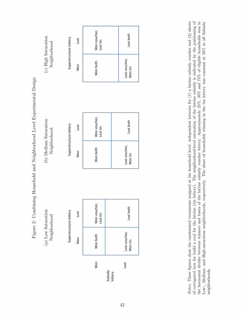
Fig

ure

2:C

ombin

ing

Hou

sehol

dan

dN

eigh

bor

hood

Lev

elE

xp

erim

enta

lD

esig

n

(a)

Low

Satu

rati

onN

eighb

orh

ood

Won

 both

Won

 vou

cher,

Lost tin

Lost vou

cher,

Won

 tin

Lost both

Supe

rstructure lottery

Subsidy 

lottery

Won

Lost

Won

Lost

(b)

Med

ium

Sat

ura

tion

Nei

ghb

orh

ood

Won

 both

Won

 vou

cher,

Lost tin

Lost vou

cher,

Won

 tin

Lost both

Supe

rstructure lottery

Won

Lost

(c)

Hig

hS

atu

rati

onN

eigh

bor

hood

Won

 both

Won

 vou

cher,

Lost tin

Lost vou

cher,

Won

 tin

Lost both

Supe

rstructure lottery

Won

Lost

Notes:

Th

ese

figu

res

show

the

ran

dom

ized

trea

tmen

tsass

igned

at

the

hou

seh

old

leve

l:in

dep

end

ent

lott

erie

sfo

r(1

)a

latr

ine

sub

sid

yvou

cher

and

(2)

shee

tsof

corr

uga

ted

iron

for

bu

ild

aro

offo

rth

ela

trin

e(t

inlo

tter

y).

Th

enei

ghb

orh

ood

-lev

elsa

tura

tion

of

the

latr

ine

sub

sid

yis

ind

icate

dby

the

posi

tion

ing

of

the

hor

izon

tal

div

ider

bet

wee

nw

inn

ers

and

lose

rsof

the

latr

ine

sub

sid

yvo

uch

erlo

tter

y.A

pp

roxim

ate

ly25%

,50%

an

d75%

of

elig

ible

hou

seh

old

sw

on

inL

ow-,

Med

ium

-an

dH

igh

-sat

ura

tion

nei

ghb

orh

ood

s,re

spec

tive

ly.

Th

esh

are

of

hou

seh

old

sw

inn

ing

inth

eti

nlo

tter

yw

as

con

stant

at

50%

inall

Su

bsi

dy

nei

ghb

orh

ood

s.

42

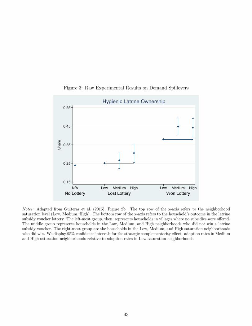
Figure 3: Raw Experimental Results on Demand Spillovers

0.15

0.25

0.35

0.45

0.55

Shar

e

No Lottery Lost Lottery Won LotteryN/A Low Medium High Low Medium High

Hygienic Latrine Ownership

Notes: Adapted from Guiteras et al. (2015), Figure 2b. The top row of the x-axis refers to the neighborhoodsaturation level (Low, Medium, High). The bottom row of the x-axis refers to the household’s outcome in the latrinesubsidy voucher lottery. The left-most group, then, represents households in villages where no subsidies were offered.The middle group represents households in the Low, Medium, and High neighborhoods who did not win a latrinesubsidy voucher. The right-most group are the households in the Low, Medium, and High saturation neighborhoodswho did win. We display 95% confidence intervals for the strategic complementarity effect: adoption rates in Mediumand High saturation neighborhoods relative to adoption rates in Low saturation neighborhoods.

43

Fig

ure

4:C

ounte

rfac

tual

pol

icy:

subsi

diz

e50

%of

hou

sehol

ds,

vary

subsi

dy

amou

nt

(a)

200

0B

DT

0.00

0.05

0.10

0.15

0.20

Effect on share purchasing

0.0

0.1

0.2

0.3

0.4

0.5

0.6

0.7

0.8

0.9

1.0

Sha

re p

urch

asin

g w

ithou

t sub

sidy

Dire

ct e

ffect

of p

rice

chan

geTo

tal e

ffect

of p

rice

chan

ge

(b)

3000

BD

T

0.00

0.05

0.10

0.15

0.20

Effect on share purchasing

0.0

0.1

0.2

0.3

0.4

0.5

0.6

0.7

0.8

0.9

1.0

Sha

re p

urch

asin

g w

ithou

t sub

sidy

Dire

ct e

ffect

of p

rice

chan

geTo

tal e

ffect

of p

rice

chan

ge

(c)

4000

BD

T

0.00

0.05

0.10

0.15

0.20

Effect on share purchasing

0.0

0.1

0.2

0.3

0.4

0.5

0.6

0.7

0.8

0.9

1.0

Sha

re p

urch

asin

g w

ithou

t sub

sidy

Dire

ct e

ffect

of p

rice

chan

geTo

tal e

ffect

of p

rice

chan

ge

(d)

3000

BD

T;

Nei

ghb

orh

ood

-Lev

elO

utc

omes

0.0

0.1

0.2

0.0

0.2

0.4

0.6

0.8

1.0

Loc

al li

near

sm

ooth

L

inea

r fit

Cov

aria

tes:

hou

seho

ld: l

and

owne

d; g

roup

: bas

elin

e la

trine

ow

ners

hip

(sha

re o

f hh.

)

Notes:

Pan

els

(a)-

(c)

plo

td

irec

t(d

ash

edli

ne)

an

dto

tal

(soli

dli

ne)

effec

tsof

sub

sid

izin

g50%

of

hou

seh

old

sby

nei

ghb

orh

ood

at

the

amou

nt

give

n(2

000

BD

T,

3000

BD

T,

4000

BD

T).

Pan

el(d

)re

pea

tsth

eex

erci

seof

Pan

el(b

)b

ut

ad

dit

ion

all

yp

lots

ou

tcom

esn

eigh

bor

hood

-by-n

eigh

borh

ood

,sh

owin

gth

at

most

nei

ghb

orh

ood

sare

inth

era

nge

wh

ere

ad

op

tion

isin

crea

sin

g.

Th

ex-a

xis

rep

rese

nts

sim

ula

ted

adop

tion

wit

hou

tsu

bsi

die

s,an

dth

eh

eight

of

the

curv

ere

pre

sents

the

sim

ula

ted

effec

tre

lati

veto

this

un

sub

sid

ized

level

of

adop

tion

.

44

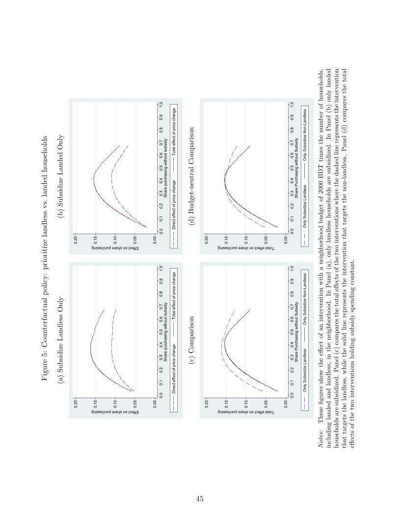
Fig

ure

5:C

ounte

rfac

tual

pol

icy:

pri

orit

ize

landle

ssvs.

landed

hou

sehol

ds

(a)

Su

bsi

diz

eL

andle

ssO

nly

0.00

0.05

0.10

0.15

0.20

Effect on share purchasing

0.0

0.1

0.2

0.3

0.4

0.5

0.6

0.7

0.8

0.9

1.0

Sha

re p

urch

asin

g w

ithou

t sub

sidy

Dire

ct e

ffect

of p

rice

chan

geTo

tal e

ffect

of p

rice

chan

ge

(b)

Su

bsi

diz

eL

and

edO

nly

0.00

0.05

0.10

0.15

0.20

Effect on share purchasing

0.0

0.1

0.2

0.3

0.4

0.5

0.6

0.7

0.8

0.9

1.0

Sha

re p

urch

asin

g w

ithou

t sub

sidy

Dire

ct e

ffect

of p

rice

chan

geTo

tal e

ffect

of p

rice

chan

ge

(c)

Com

par

ison

0.00

0.05

0.10

0.15

0.20

Total effect on share purchasing

0.0

0.1

0.2

0.3

0.4

0.5

0.6

0.7

0.8

0.9

1.0

Sha

re P

urch

asin

g w

ithou

t Sub

sidy

Onl

y S

ubsi

dize

Lan

dles

sO

nly

Sub

sidi

ze N

on-L

andl

ess

(d)

Bu

dge

t-n

eutr

alC

ompar

ison

0.00

0.05

0.10

0.15

0.20

Total effect on share purchasing

0.0

0.1

0.2

0.3

0.4

0.5

0.6

0.7

0.8

0.9

1.0

Sha

re P

urch

asin

g w

ithou

t Sub

sidy

Onl

y S

ubsi

dize

Lan

dles

sO

nly

Sub

sidi

ze N

on-L

andl

ess

Notes:

Th

ese

figu

res

show

the

effec

tof

an

inte

rven

tion

wit

ha

nei

ghb

orh

ood

bu

dget

of

2000

BD

Tti

mes

the

nu

mb

erof

hou

seh

old

s,in

clu

din

gla

nd

edan

dla

nd

less

,in

the

nei

ghb

orh

ood

.In

Pan

el(a

),on

lyla

nd

less

hou

seh

old

sare

sub

sid

ized

.In

Pan

el(b

)on

lyla

nd

edh

ouse

hol

ds

are

sub

sid

ized

.P

anel

(c)

com

pare

sth

eto

taleff

ects

ofth

etw

oin

terv

enti

on

sw

her

eth

ed

ash

edli

ne

rep

rese

nts

the

inte

rven

tion

that

targ

ets

the

lan

dle

ss,

wh

ile

the

soli

dli

ne

rep

rese

nts

the

inte

rven

tion

that

targ

ets

the

non

-lan

dle

ss.

Pan

el(d

)co

mp

are

sth

eto

tal

effec

tsof

the

two

inte

rven

tion

sh

old

ing

sub

sid

ysp

end

ing

con

stant.

45

Figure 6: Intensive (Price) Margin vs. Extensive (Scope) MarginAcross Neighborhoods

(a) Naıve experiment: Budget varies

0.00

0.05

0.10

0.15

0.20To

tal e

ffect

on

shar

e pu

rcha

sing

0.0 0.1 0.2 0.3 0.4 0.5 0.6 0.7 0.8 0.9 1.0Share Purchasing without Subsidy

100% get 1000 BDT 50% get 2000 25% get 4000

(b) Budget-neutral Experiment

0.00

0.05

0.10

0.15

0.20

Tota

l effe

ct o

n sh

are

purc

hasi

ng

0.0 0.1 0.2 0.3 0.4 0.5 0.6 0.7 0.8 0.9 1.0Share Purchasing without Subsidy

100% get 1000 BDT 50% get 1372 25% get 1812

Notes: These graphs compare the total effects of interventions trading off subsidy amount againstscope (the share of neighborhoods where subsidies are offered). The top panel (6a) compares:offering a 1000 BDT subsidy in 100% of neighborhoods (short-dashed line); 2000 BDT in 50%(long-dashed line); 4000 BDT subsidy in 25% (solid line). The bottom panel (6b) adjusts thesubsidy amounts so that the cost per neighborhood is constant across the three interventions. Inall cases, all households in subsidy neighborhoods are offered subsidies.

46

Figure 7: Intensive (Price) Margin vs. Extensive (Saturation) MarginWithin Neighborhoods

(a) Naıve experiment: Budget varies

0.00

0.05

0.10

0.15

0.20

Tota

l effe

ct o

n sh

are

purc

hasi

ng

0.0 0.1 0.2 0.3 0.4 0.5 0.6 0.7 0.8 0.9 1.0Share Purchasing without Subsidy

100% get 1000 BDT 50% get 2000 25% get 4000

(b) Budget-neutral experiment

0.00

0.05

0.10

0.15

0.20

Tota

l effe

ct o

n sh

are

purc

hasi

ng

0.0 0.1 0.2 0.3 0.4 0.5 0.6 0.7 0.8 0.9 1.0Share Purchasing without Subsidy

100% get 1000 BDT 50% get 1479 BDT 25% get 2105 BDT

Notes: These graphs compare the total effect of interventions trading of subsidy amount againstsaturation (the share of households subsidized by neighborhood). The top panel (7a) compares:offering a 1000 BDT subsidy to 100% of households (short-dashed line); 2000 BDT to 50% (long-dashed line); 4000 BDT subsidy to 25% (solid line). The bottom panel (7b) adjusts the subsidyamounts so that the cost per neighborhood is constant across the three interventions.

47

Figure 8: Targeting Densely Populated Neighborhoods

(a) Subsidy: 2000 BDT per household

0.00

0.05

0.10

0.15

0.20To

tal e

ffec

t on

shar

e pu

rcha

sing

0.0 0.1 0.2 0.3 0.4 0.5 0.6 0.7 0.8 0.9 1.0Share Purchasing without Subsidy

20th Percentile 50th Percentile 80th Percentile

(b) Subsidy: 4000 BDT per household

0.00

0.05

0.10

0.15

0.20

Tota

l eff

ect o

n sh

are

purc

hasi

ng

0.0 0.1 0.2 0.3 0.4 0.5 0.6 0.7 0.8 0.9 1.0Share Purchasing without Subsidy

20th Percentile 50th Percentile 80th Percentile

Notes: These graphs compare the effects of interventions targeting neighborhoods of the 20thquantile (short-dashed line), the 50th quantile (long-dashed line), and the 80th quantile (solid line)of the density distribution. The top panel (8a) shows results offering a 2000 BDT subsidy to 50%of households, by neighborhood; The bottom panel (8b) is similar, but with a 4000 BDT subsidy.

48

Figure 9: Targeting 4000 BDT Subsidies to Households with Specific Network Positions

(a) Parents of Children’s Playmates

0.00

0.05

0.10

0.15

0.20

Tota

l effe

ct o

n sh

are

purc

hasi

ng

0.0 0.1 0.2 0.3 0.4 0.5 0.6 0.7 0.8 0.9 1.0Share Purchasing without Subsidy

20th Percentile 90th Percentile

(b) Leader Contacts (Those who Resolve Disputes)

0.00

0.05

0.10

0.15

0.20

Tota

l effe

ct o

n sh

are

purc

hasi

ng

0.0 0.1 0.2 0.3 0.4 0.5 0.6 0.7 0.8 0.9 1.0Share Purchasing without Subsidy

20th Percentile 90th Percentile

(c) Contacts approached for Technical Advice

0.00

0.05

0.10

0.15

0.20

Tota

l effe

ct o

n sh

are

purc

hasi

ng

0.0 0.1 0.2 0.3 0.4 0.5 0.6 0.7 0.8 0.9 1.0Share Purchasing without Subsidy

20th Percentile 90th Percentile

Notes: These graphs compare the effects of subsidizing other households with a specific connection to the indexhousehold, on the index household’s adoption choice. In Table 5 we measure connection in terms of the proportion ofhouseholds contacts who won latrine vouchers, and two lines display the 20th and 90th percentiles of this proportion.The top panel (9a) shows the effects of subsidizing kids’ playmates’ parents; the middle panel (9b) subsidizes thoseperceived as leaders; and the bottom panel (9c) target those the index households would approach for advice abouta new technology. Subsidies assigned to contacts is always 4000 BDT in all these simulations.49

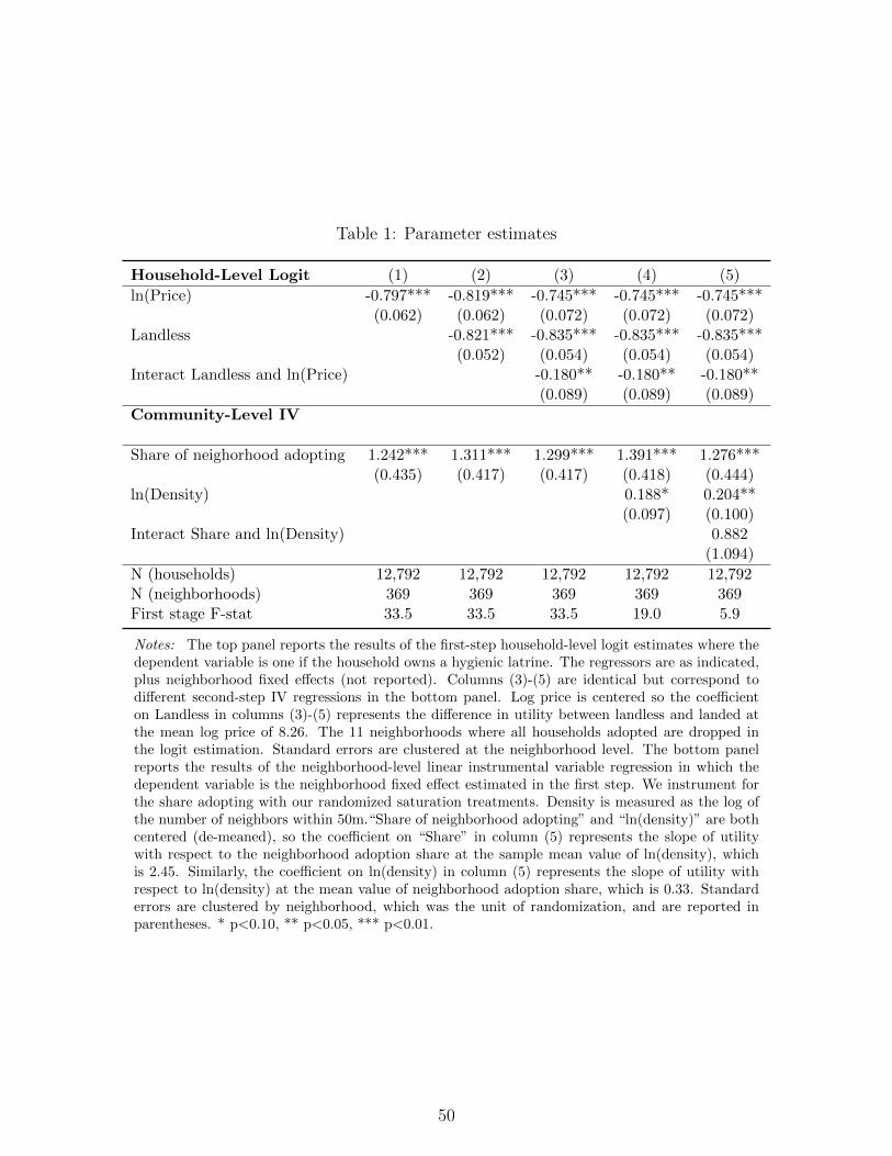
Table 1: Parameter estimates

Household-Level Logit (1) (2) (3) (4) (5)

ln(Price) -0.797*** -0.819*** -0.745*** -0.745*** -0.745***(0.062) (0.062) (0.072) (0.072) (0.072)

Landless -0.821*** -0.835*** -0.835*** -0.835***(0.052) (0.054) (0.054) (0.054)

Interact Landless and ln(Price) -0.180** -0.180** -0.180**(0.089) (0.089) (0.089)

Community-Level IV

Share of neighorhood adopting 1.242*** 1.311*** 1.299*** 1.391*** 1.276***(0.435) (0.417) (0.417) (0.418) (0.444)

ln(Density) 0.188* 0.204**(0.097) (0.100)

Interact Share and ln(Density) 0.882(1.094)

N (households) 12,792 12,792 12,792 12,792 12,792N (neighborhoods) 369 369 369 369 369First stage F-stat 33.5 33.5 33.5 19.0 5.9

Notes: The top panel reports the results of the first-step household-level logit estimates where thedependent variable is one if the household owns a hygienic latrine. The regressors are as indicated,plus neighborhood fixed effects (not reported). Columns (3)-(5) are identical but correspond todifferent second-step IV regressions in the bottom panel. Log price is centered so the coefficienton Landless in columns (3)-(5) represents the difference in utility between landless and landed atthe mean log price of 8.26. The 11 neighborhoods where all households adopted are dropped inthe logit estimation. Standard errors are clustered at the neighborhood level. The bottom panelreports the results of the neighborhood-level linear instrumental variable regression in which thedependent variable is the neighborhood fixed effect estimated in the first step. We instrument forthe share adopting with our randomized saturation treatments. Density is measured as the log ofthe number of neighbors within 50m.“Share of neighborhood adopting” and “ln(density)” are bothcentered (de-meaned), so the coefficient on “Share” in column (5) represents the slope of utilitywith respect to the neighborhood adoption share at the sample mean value of ln(density), whichis 2.45. Similarly, the coefficient on ln(density) in column (5) represents the slope of utility withrespect to ln(density) at the mean value of neighborhood adoption share, which is 0.33. Standarderrors are clustered by neighborhood, which was the unit of randomization, and are reported inparentheses. * p<0.10, ** p<0.05, *** p<0.01.

50

Table 2: Targeting Socially Central Households

(1) (2) (3)

Share of neighborhood adopting 1.293∗∗ 1.323∗∗ 1.373∗

(0.418) (0.411) (0.550)

Neighborhood where Highly Connected -0.014 -0.013Households (HCH) were Targeted with Subsidies (0.061) (0.062)

Interact share and HCH -0.103(0.824)

First-stage F stat. 33.6 33.6 17.0Num. neighborhoods 368 368 368

Notes: The table reports results of the second step IV estimates where the dependent variableis the neighborhood level fixed effect from the first step household-level logit. The first step logitincludes log price, an indicator for landless and the interaction of the two, corresponding to column(3) in the top panel of Table 1. The instruments are indicators for our randomized saturationtreatments and, in column (3), their interaction with the randomized treatment targeting highlyconnected households (HCH). The share of the neighborhood adopting is recentered (mean zero)so the coefficient on the randomized HCH treatment in column (3) represents the slope of utilitywith respect to the HCH treatment at the sample mean value of the neighborhood adoption share,which is 0.333. Standard errors are clustered by neighborhood, which is the unit of randomization,and are reported in parentheses. * p<0.10, ** p<0.05, *** p<0.01.

51

Table 3: Reduced Form Regressions of Household Responsesto Lottery Outcomes, Subsidy Saturation and HCH Targeting

(1) (2)Neighborhoods where

HCHs Targetedwith Subsidies

Neighborhoods whereHCHs were not Targeted

with Subsidies

Household-Level LotteryOutcomes

Only won latrine 0.111∗∗∗ 0.072∗∗∗

(0.025) (0.024)

Only won tin 0.023 -0.021(0.028) (0.028)

Won both 0.213∗∗∗ 0.172∗∗∗

(0.023) (0.026)

Neighborhood-Level SubsidySaturation Treatments

Medium (50% Subsidy) 0.048 0.058∗

Saturation Treatment (0.031) (0.034)

High (75% Subsidy) 0.040 0.100∗∗

Saturation Treatment (0.032) (0.040)

Mean ownership %, excluded group 24 32Num. of neighborhoods 123 102Num. of households 4,266 3,362

Notes: The table presents results from household-level OLS regressions where the samples aresplit into subsidy neighborhoods assigned to the randomized treatment targeting socially centralhouseholds (HCH, column (1)), and subsidy neighborhoods not receiving this treatment (i.e., alleligible households having an equal chance of winning, Column (2)). Regressors indicate whetherthe households won the latrine, tin, or both, as well as whether they were in Medium (50%) SubsidySaturation treatment neighborhoods or High (75%) Subsidy Saturation treatment neighborhoods.The excluded group consists of households that lost both lotteries in the neighborhoods randomlyassigned to the Low (25%) Subsidy Saturation treatment. Standard errors are clustered by neig-hborhood, which is the unit of randomization, and are reported in parentheses. * p<0.10, **p<0.05, *** p<0.01.

52

Table 4: Reduced Form Household-level OLSDependent Variable: Ownership of Hygienic Latrine

Neighborhood targeting treatment: HCH Non-HCH

Household lottery outcome: Won Lottery Lost Lottery Won Lottery Lost Lottery

Neighborhood Subsidy Saturation

Medium 0.052 0.038 0.105∗∗∗ -0.010(0.040) (0.032) (0.040) (0.039)

High 0.036 0.034 0.127∗∗∗ 0.067(0.039) (0.035) (0.043) (0.048)

Mean excluded ownership % 42 27 36 29Num. of neighborhoods 123 123 102 102Num. of households 2,760 1,506 2,130 1,232

Notes: This table presents results of household-level OLS regressions where the sample is splitfirst by whether the neighborhood was assigned to the “HCH” (“highly connected households”)treatment, in which socially central households were over-weighted in the latrine subsidy lottery. Incolumns (1) and (2), the sample consists of neighborhoods assigned to the HCH treatment, whilein columns (3) and (4), the sample consists of neighborhoods where the lottery was unweighted(“Non-HCH”). Second, the sample is further divided by whether the household won (columns (1)and (3)) or lost (columns (2) and (4)) the latrine subsidy lottery. The regressors are indicators forthe neighborhood’s level of subsidy saturation. The sample consists of all eligible households insubsidy villages, so the excluded category consists of eligible households in low-subsidy-saturationneighborhoods. Standard errors are clustered by neighborhood, which is the unit of randomization,and are reported in parentheses. * p<0.10, ** p<0.05, *** p<0.01.

53

Table 5: First-step Household-level Fixed Effects LogitDependent Variable: Ownership of Hygienic Latrine

(1) (2) (3)Resolve Technical Playmate

Price (log) -0.821∗∗∗ -0.785∗∗∗ -0.814∗∗∗

(0.075) (0.091) (0.077)Price (log) × % of Resolve contacts who won lottery 0.090

(0.162)% of Resolve contacts who won lottery -0.203∗

(0.112)Price (log) × % of Technical contacts who won lottery -0.016

(0.140)% of Technical contacts who won lottery 0.234∗∗

(0.115)Price (log) × % of Playmate contacts who won lottery 0.064

(0.142)% of Playmate contacts who won lottery 0.052

(0.092)

Num. of neighborhoods 369 369 369Num. of households 12,824 12,824 12,824

Notes: The table reports the results of the first-step logit estimates where the dependent variable isone if the household owns a hygienic latrine. The regressors are the share of neighborhood contactsthat randomly received a voucher. Column (1) includes the share of contacts the household wouldgo to for conflict resolution; column (2) includes the share of contacts the household would go tofor technical advice; and column (3) includes the share of contacts that have children that theirown children play with. The price variable is recentered with the mean at zero; the true mean oflog price is 8.26. * p<0.10, ** p<0.05, *** p<0.01.

54

A Appendix Tables

Table A1: Descriptive Statistics and Balance – Neighborhood-Level Treatments

Neighborhood Intensity Treatment: All No Subsidy Low Intensity Medium Intensity High Intensity Joint

Mean Mean Mean Diff Mean Diff Mean Diff p-val.(S.D.) (S.D.) (S.D.) [S.E.] (S.D.) [S.E.] (S.D.) [S.E.]

(1) (2) (3) (4) (5) (6) (7) (8) (9)

Neighborhood characteristics:

Share w. access to latrine 0.784 0.773 0.793 0.020 0.786 0.013 0.792 0.019 0.888(0.219) (0.222) (0.199) [0.029] (0.224) [0.031] (0.230) [0.032]

Share w. access to hygienic latrine 0.426 0.405 0.451 0.045 0.424 0.018 0.443 0.038 0.524(0.240) (0.240) (0.248) [0.035] (0.231) [0.033] (0.244) [0.034]

Share that owns any latrine 0.562 0.554 0.570 0.017 0.556 0.002 0.578 0.024 0.856(0.217) (0.210) (0.210) [0.030] (0.224) [0.031] (0.231) [0.031]

Share that owns a hygienic latrine 0.309 0.289 0.329 0.040 0.303 0.014 0.334 0.044 0.354(0.202) (0.191) (0.212) [0.029] (0.197) [0.027] (0.218) [0.029]

Share of households who openly defecate 0.357 0.360 0.346 −0.014 0.333 −0.027 0.388 0.029 0.611(0.256) (0.251) (0.237) [0.034] (0.263) [0.036] (0.274) [0.037]

Share of landless households 0.466 0.474 0.429 −0.045∗ 0.457 −0.018 0.496 0.022 0.106(0.190) (0.203) (0.170) [0.026] (0.194) [0.028] (0.176) [0.026]

Density (mean number of households within 50 meters) 12.2 12.1 12.3 0.2 12.4 0.3 12.0 −0.0 0.940(4.7) (4.9) (4.6) [0.7] (4.3) [0.6] (4.9) [0.7]

Number of households 48.1 49.1 48.9 −0.3 47.0 −2.1 46.6 −2.5 0.604(15.7) (15.2) (15.0) [2.1] (16.9) [2.3] (15.9) [2.2]

Number of eligible households 36.1 37.1 35.7 −1.4 35.4 −1.7 35.3 −1.8 0.711(13.0) (13.3) (12.3) [1.8] (13.6) [1.9] (12.7) [1.8]

Household characteristics (among subsidy-eligible households):

Household head is female 0.103 0.104 0.099 −0.005 0.100 −0.004 0.110 0.006 0.567(0.304) (0.305) (0.298) [0.007] (0.300) [0.009] (0.313) [0.008]

Age of household head 40.4 40.4 40.4 0.0 40.6 0.3 40.5 0.2 0.858(13.2) (13.4) (12.9) [0.4] (13.3) [0.3] (13.2) [0.4]

Schooling of the household head (years) 5.3 5.3 5.5 0.2 5.3 −0.0 5.3 −0.0 0.723(4.8) (4.7) (5.0) [0.2] (4.8) [0.2] (4.8) [0.2]

Household head is Muslim 0.834 0.833 0.807 −0.027 0.861 0.027 0.835 0.002 0.784(0.372) (0.373) (0.395) [0.051] (0.346) [0.043] (0.371) [0.048]

Household head is Bengali 0.877 0.872 0.830 −0.042 0.913 0.041 0.894 0.022 0.378(0.329) (0.334) (0.376) [0.049] (0.282) [0.037] (0.308) [0.042]

Household head works in agriculture 0.705 0.715 0.708 −0.007 0.678 −0.037∗ 0.711 −0.004 0.342(0.456) (0.451) (0.455) [0.020] (0.467) [0.021] (0.454) [0.018]

Decimals of land owned by household head 7.4 7.0 8.3 1.3∗∗ 7.9 0.9∗ 6.9 −0.1 0.055∗

(15.2) (12.6) (21.9) [0.7] (14.7) [0.5] (12.2) [0.5]

Number of Proper meals during Monga 0.523 0.552 0.523 −0.029 0.536 −0.016 0.453 −0.099∗∗∗ 0.018∗∗

(0.499) (0.497) (0.500) [0.032] (0.499) [0.031] (0.498) [0.032]

Household members w. diarrhea in the last 1 week 0.053 0.048 0.057 0.008 0.056 0.008 0.055 0.006 0.612(0.224) (0.215) (0.231) [0.008] (0.230) [0.007] (0.228) [0.007]

Access to piped water or tube well all year 0.895 0.908 0.848 −0.060∗∗ 0.922 0.014 0.884 −0.024 0.081∗

(0.307) (0.289) (0.359) [0.029] (0.268) [0.021] (0.320) [0.023]

Observation counts:

Number of neighborhoods 381 150 74 77 77

Number of households 19,878 7,366 3,615 3,619 3,587

Number of eligible households 13,708 5,562 2,644 2,728 2,718

Notes: This table presents summary statistics (means and standard deviations) of key baseline varia-bles for all neighborhoods (Column 1), for no-subsidy neighborhoods (i.e., Control, LPP Only and SupplyOnly; see text for definitions) (Col. 2), and for neighborhoods assigned to the low-saturation (Col. 3),medium-saturation (Col. 5) and high-saturation (Col. 7) subsidy treatments. For the low-, medium-, andhigh-saturation groups, we present pairwise differences in means relative to the no-subsidy group in Co-lumns 4, 6, and 8 respectively. Column 9 shows the p-value from an F-test of the joint significance of thetreatment indicators (low, medium, and high intensity). Standard deviations are in parentheses, and theestimated standard errors are in brackets. Standard errors for household-level regressions are clustered atthe neighborhood level. * p<0.10, ** p<0.05, *** p<0.01.

A1

Table A2: Descriptive Statistics and Balance – Household Subsidy Lotteries

Household Lottery Treatment: All Lost Both Latrine only Tin only Won both Joint

Mean Mean Mean Diff Mean Diff Mean Diff p-val.(S.D.) (S.D.) (S.D.) [S.E.] (S.D.) [S.E.] (S.D.) [S.E.]

(1) (2) (3) (4) (5) (6) (7) (8) (9)

Share w. access to any latrine 0.780 0.799 0.789 −0.010 0.773 −0.025 0.764 −0.035∗ 0.278(0.414) (0.401) (0.408) [0.020] (0.419) [0.023] (0.425) [0.020]

Share w. access to hygienic latrine 0.437 0.442 0.440 −0.002 0.438 −0.004 0.432 −0.010 0.974(0.496) (0.497) (0.497) [0.024] (0.496) [0.028] (0.496) [0.024]

Share that owns any latrine 0.572 0.594 0.581 −0.013 0.560 −0.034 0.558 −0.036 0.394(0.495) (0.491) (0.494) [0.024] (0.497) [0.028] (0.497) [0.024]

Share that owns a hygienic latrine 0.327 0.330 0.335 0.006 0.326 −0.004 0.318 −0.012 0.845(0.469) (0.470) (0.472) [0.023] (0.469) [0.026] (0.466) [0.023]

Share of households who openly defecate 0.371 0.341 0.376 0.034 0.382 0.041 0.378 0.037 0.343(0.483) (0.474) (0.484) [0.023] (0.486) [0.027] (0.485) [0.023]

Share of landless households 0.457 0.424 0.472 0.049∗∗∗ 0.468 0.045∗∗ 0.454 0.030∗ 0.019∗∗

(0.498) (0.494) (0.499) [0.016] (0.499) [0.018] (0.498) [0.016]

Neighb. avg. num. of HHs within 50m 12.4 12.5 12.2 −0.3∗ 12.6 0.1 12.3 −0.2 0.085∗

(4.6) (4.8) (4.5) [0.2] (4.8) [0.2] (4.4) [0.1]

Household head is female 0.103 0.126 0.085 −0.041∗∗∗ 0.133 0.007 0.091 −0.034∗∗∗ 0.000∗∗∗

(0.304) (0.331) (0.279) [0.010] (0.340) [0.012] (0.288) [0.010]

Age of household head 40.5 41.2 40.4 −0.9∗∗ 41.0 −0.2 39.9 −1.3∗∗∗ 0.006∗∗∗

(13.1) (13.5) (13.1) [0.4] (13.5) [0.5] (12.6) [0.4]

Schooling of the household head (years) 5.4 5.3 5.4 0.1 5.3 −0.0 5.3 −0.0 0.834(4.9) (5.0) (4.8) [0.2] (5.0) [0.2] (4.8) [0.2]

Household head is Muslim 0.829 0.845 0.835 −0.010 0.825 −0.020 0.817 −0.028∗∗ 0.102(0.377) (0.362) (0.372) [0.012] (0.380) [0.014] (0.387) [0.012]

Household head is Bengali 0.874 0.881 0.879 −0.001 0.865 −0.016 0.869 −0.011 0.410(0.332) (0.324) (0.326) [0.011] (0.342) [0.012] (0.337) [0.011]

Household head works in agriculture 0.700 0.673 0.714 0.041∗∗∗ 0.655 −0.019 0.726 0.052∗∗∗ 0.000∗∗∗

(0.458) (0.469) (0.452) [0.015] (0.476) [0.017] (0.446) [0.015]

Decimals of land owned by household head 7.7 8.3 7.0 −1.3∗∗ 7.8 −0.6 8.0 −0.3 0.013∗∗

(16.7) (19.6) (11.6) [0.6] (23.5) [0.8] (14.4) [0.6]

Number of Proper meals during Monga 0.502 0.501 0.504 0.003 0.471 −0.029 0.516 0.016 0.056∗

(0.500) (0.500) (0.500) [0.016] (0.499) [0.019] (0.500) [0.016]

Household members w. diarrhea in the last 1 week 0.056 0.057 0.059 0.002 0.059 0.002 0.051 −0.006 0.582(0.230) (0.232) (0.236) [0.008] (0.236) [0.009] (0.221) [0.007]

Access to piped water or tube well all year 0.886 0.864 0.902 0.038∗∗∗ 0.873 0.009 0.890 0.026∗∗ 0.001∗∗∗

(0.318) (0.343) (0.298) [0.011] (0.333) [0.013] (0.313) [0.011]

Observation counts:

Number of households 8,146 1,507 2,539 1,431 2,669

Notes: This table presents summary statistics (means and standard deviations) of key baseline variablesfor all households participating in the subsidy lotteries (Column 1), for households who lost both lotteries(Col. 2), and for households who won the latrine only (Col. 3), the tin only (Col. 5), and won both latrineand tin (Col. 7). For the households who won the latrine only, tin only, and won both we present pairwisedifferences in means relative to the group of households that lost both in Columns 4, 6, and 8 respectively.Column 9 shows the p-value from an F-test of the joint significance of the household lottery outcomes (wonlatrine only, tin only, and both). Standard deviations are in parentheses, and the estimated standard errorsare in brackets. Standard errors robust to heteroskedasticity. * p<0.10, ** p<0.05, *** p<0.01.

A2

Table A3: Structural Estimates for “Fixed Share” Subsidy neighborhoods(omitting “Early Adopter” Subsidy Neighborhoods)

Household-Level Logit (1) (2) (3) (4) (5)ln(Price) -0.722*** -0.752*** -0.639*** -0.639*** -0.639***

(0.084) (0.084) (0.103) (0.103) (0.103)Landless 0.823*** -0.839*** -0.839*** -0.839***

(0.066) (0.068) (0.068) (0.068)Interact Landless and ln(Price) -0.271** -0.271** -0.271**

(0.089) (0.089) (0.089)Community-Level IV

Share of neighorhood adopting 1.754*** 1.828*** 1.779*** 1.971*** 1.980***(0.475) (0.448) (0.453) (0.420) (0.420)

ln(Density) 0.094 0.089(0.099) (0.094)

Interact Share and ln(Density) -0.412(0.822)

N (households) 8,892 8,892 8,892 8,892 8,892N (neighborhoods) 256 256 256 256 256First-step F-stat 21.4 21.4 21.4 11.7 8.1

Notes: This table shows the first-step household-level logit estimates, and the neighborhood-level linearinstrumental variable regression for neighborhoods that received the Fixed Share treatment. The top panelreports the results of the first-step household-level logit estimates where the dependent variable is one ifthe household owns a hygienic latrine. The regressors are as indicated, plus neighborhood fixed effects (notreported). Columns (3)-(5) are identical but correspond to different second-step IV regressions in the bottompanel. Log price is centered so the coefficient on Landless in columns (3)-(5) represents the difference inutility between landless and landed at the mean log price of 8.45. The 11 neighborhoods where all householdsadopted are dropped in the logit estimation. Standard errors are clustered at the neighborhood level. Thebottom panel reports the results of the neighborhood-level linear instrumental variable regression in whichthe dependent variable is the neighborhood fixed effect. We instrument for the share adopting with ourrandomized saturation treatments. In columns (1)-(3) th neighborhood fixed effect is estimated with thefirst-stage regressors indicated in the top panel. Density is measured as the log of the number of neighborswithin 50m. Density is centered so the coefficient represents the differerence in utility at the mean log densityof 2.45. * p<0.10, ** p<0.05, *** p<0.01.

A3

Table A4: Sensitivity to Leaving out Own Household’s Adoption Decision fromConstruction of “Neighborhood Share” variable.

Dependent Variable: Ownership of Hygienic Latrine.Estimation Method: One-Step Household-Level 2SLS

(1) (2)

Price (log) -0.147∗∗∗ -0.148∗∗∗

(0.012) (0.012)

Share of neighborhood adopting 0.311∗∗∗

(0.083)

Share of neighborhood adopting leaving household out 0.302∗∗∗

(0.082)

Landless Household -0.158∗∗∗ -0.159∗∗∗

(0.010) (0.010)

Mean ownership %, excluded group 24 24Num. of neighborhoods 378 378Num. of households 13,008 13,008

Notes: The table reports results of the one-step household-level 2SLS estimates with theshare of the neighborhood that owns a latrine is measured with and without the householdincluded. Both the share of the neighborhood that owns a hygienic latrine with and withoutthe household included is instrumented with the neighborhood-level treatment variable andare recentered so the mean is zero. The log of price is instrumented with the household-levellottery treatment variable and is centered (mean zero). Standard errors are clustered at theneighborhood level which was the unit of randomization and are in parentheses. * p<0.10,** p<0.05, *** p<0.01.

A4

Table A5: Reduced Form Household-level OLS for Landless and Landed SubsamplesDependent Variable: Ownership of Hygienic Latrine

(1) (2)Landless Only Landed Only

Household-Level LotteryOutcomes

Only won latrine 0.103∗∗∗ 0.098∗∗∗

(0.022) (0.024)

Only won tin 0.013 0.013(0.023) (0.028)

Won both 0.216∗∗∗ 0.186∗∗∗

(0.022) (0.023)

Neighborhood-Level SubsidySaturation Treatments

Medium (50% Subsidy) 0.072∗∗∗ 0.042Saturation Treatment (0.026) (0.027)

High (75% Subsidy) 0.080∗∗∗ 0.070∗∗

Saturation Treatment (0.028) (0.028)

Mean ownership %, excluded group 14 36Num. of neighborhoods 225 224Num. of households 3,408 4,220

Notes: The table presents results from household-level OLS regressions where the samplesare split into landless households (Column (1)), and landed households (Column (2)). Re-gressors indicate whether the households won the latrine, tin, or both, as well as whetherthey were in Medium (50%) Subsidy Saturation treatment neighborhoods or High (75%)Subsidy Saturation treatment neighborhoods. The excluded group consists of householdsthat lost both lotteries in the neighborhoods randomly assigned to the Low (25%) SubsidySaturation treatment. Standard errors are clustered by neighborhood, which is the unit ofrandomization, and are in parentheses. * p<0.10, ** p<0.05, *** p<0.01.

A5

Table A6: Comparing Voucher Lottery Winners in the HCH and non-HCH Treatments

HCH Treatment Status: HCH Non-HCH

Mean Mean Diff p-val.(S.D.) (S.D.) [S.E.]

(1) (2) (3) (4)

Household owns any latrine at baseline 0.585 0.549 0.036 0.257(0.493) (0.498) [0.032]

Household owns a hygienic latrine at baseline 0.343 0.306 0.037 0.235(0.475) (0.461) [0.031]

Adults in household openly defecate at baseline 0.370 0.384 −0.014 0.731(0.483) (0.487) [0.040]

Household owns land 0.541 0.535 0.007 0.795(0.498) (0.499) [0.025]

Number of households within 50m 13.1 11.9 1.2 0.104(7.7) (7.2) [0.7]

Household head is female 0.081 0.097 −0.016∗ 0.087∗

(0.273) (0.296) [0.009]

Age of household head 40.2 40.1 0.0 0.958(12.7) (13.1) [0.5]

Schooling of the household head (years) 5.4 5.4 0.0 0.919(4.8) (4.9) [0.2]

Household head works in agriculture 0.727 0.709 0.018 0.391(0.445) (0.454) [0.021]

Decimals of land owned by household head 7.5 7.6 −0.1 0.831(13.3) (12.9) [0.5]

Number of Proper meals during Monga 0.538 0.477 0.061∗ 0.057∗

(0.499) (0.500) [0.032]

Household members w. diarrhea in the last 1 week 0.053 0.058 −0.005 0.594(0.225) (0.234) [0.009]

Access to piped water or tube well all year 0.892 0.906 −0.014 0.517(0.310) (0.292) [0.021]

Outdegree score 7.5 7.5 −0.0 0.955(3.0) (2.7) [0.3]

Indegree score 8.3 7.1 1.2∗∗ 0.022∗∗

(15.7) (15.1) [0.5]

Eigenvector centrality 0.052 0.054 −0.002 0.636(0.053) (.051) [0.005]

Between centrality 0.008 0.006 0.002 0.173(0.370) (0.034) [0.001]

Observation counts:

Number of households 5,208 2,930 2,262

Notes: This table presents summary statistics (means and standard deviations) of key varia-bles measured at baseline for voucher winners in all neighborhoods (Column 1), neighborhoodswhere the lottery was biased towards highly connected households (Column 2), and neighbor-hoods that were not biased (Column 3). We present differences in means in Column 4 withestimated standard errors clustered at the neighborhood level. Column 5 shows the p-valuesand significance levels. * p<0.10, ** p<0.05, *** p<0.01.

A6