EC611--Managerial Economics

Demand and Supply

Dr. Savvas C Savvides, European University Cyprus

1

Some key terms

Marketa set of arrangements by which buyers and sellers are in contact to exchange goods or services

Demandthe quantity of a good buyers wish to purchase at each conceivable price

Supplythe quantity of a good sellers wish to sell at each conceivable price

Equilibrium priceprice at which quantity supplied = quantity demanded

2

What, How and for Whom

The market:determines what goods are being produced

• there may be goods for which no consumer is prepared to pay a price at which firms would be willing to supply

decides how much of a good should be produced

• by finding the price at which the quantity demanded equals the quantity supplied

tells us for whom the goods are produced

• those consumers willing to pay the equilibrium price

3

Law of Demand

A decrease in the price of a good, all other things held constant, will cause an increase in the quantity demanded of the good.An increase in the price of a good, all other things held constant, will cause a decrease in the quantity demanded of the good.

Quantity Demanded: The amount purchased at a particular price for a given time period

4

Law of Demand

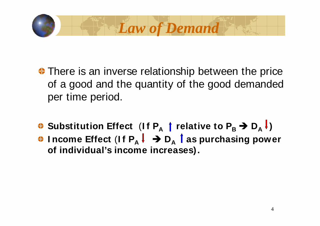
There is an inverse relationship between the price of a good and the quantity of the good demanded per time period.

Substitution Effect (If PA relative to PB DA )Income Effect (If PA DA as purchasing power of individual’s income increases).

5

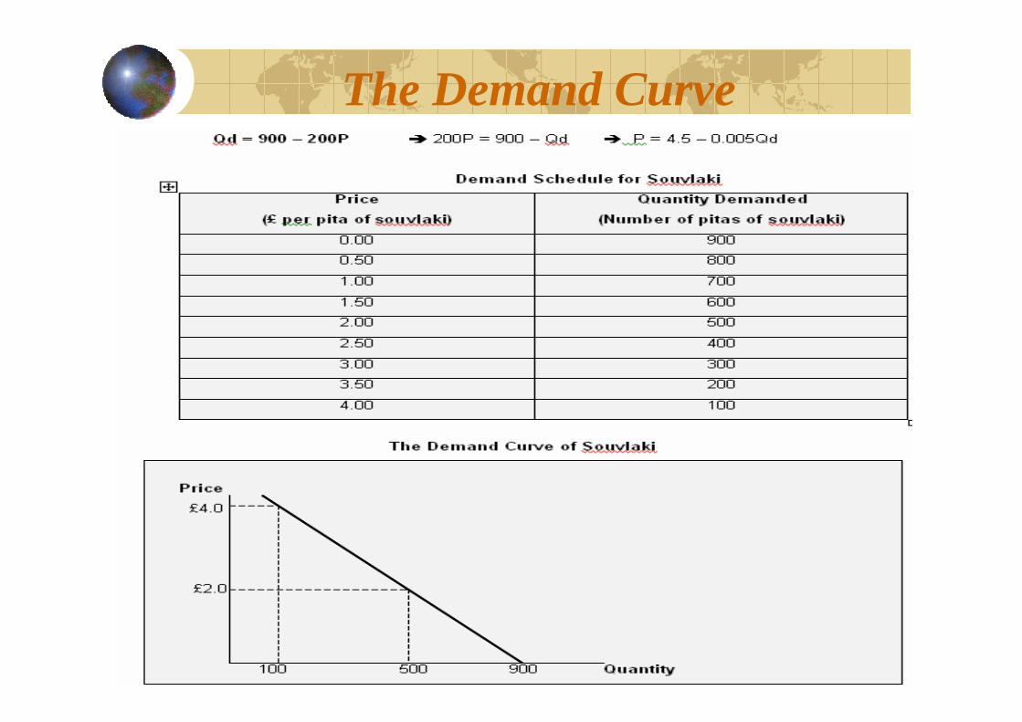
The Demand Curve

6

The Demand Curve

Quantity

Price

P0

Q0

P1

Q1

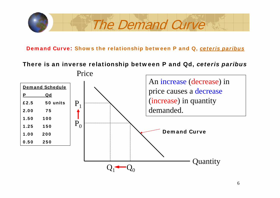
An increase (decrease) in price causes a decrease(increase) in quantity demanded.

Demand Curve: Shows the relationship between P and Q, ceteris paribus

Demand Schedule

P Qd

£2.5 50 units

2.00 75

1.50 100

1.25 150

1.00 200

0.50 250

Demand Curve

There is an inverse relationship between P and Qd, ceteris paribus

7

Changes in Demand

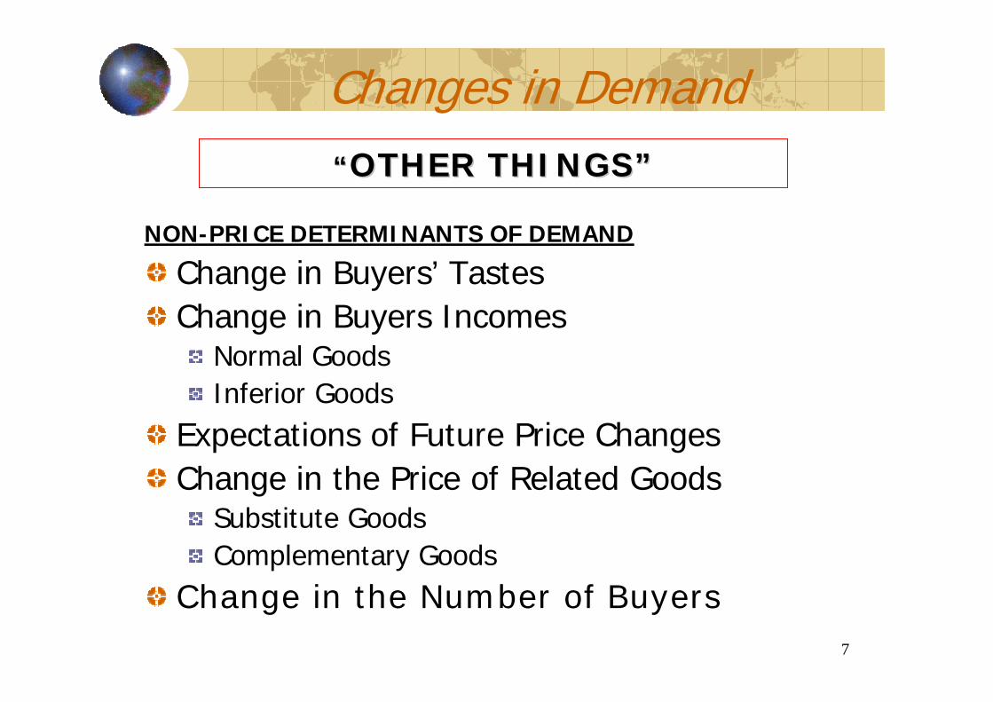
NON-PRICE DETERMINANTS OF DEMAND

Change in Buyers’ TastesChange in Buyers Incomes

Normal GoodsInferior Goods

Expectations of Future Price ChangesChange in the Price of Related Goods

Substitute GoodsComplementary Goods

Change in the Number of Buyers

““OTHER THINGSOTHER THINGS””

8

Change in Demand

Quantity

Price

P0

Q0 Q1

An increase (decrease) in demand refers to a rightward (leftward)shift in the market demand curve.

A change in any of the “other things” will affect the position of Demand

D0D2

D1

Q2

9

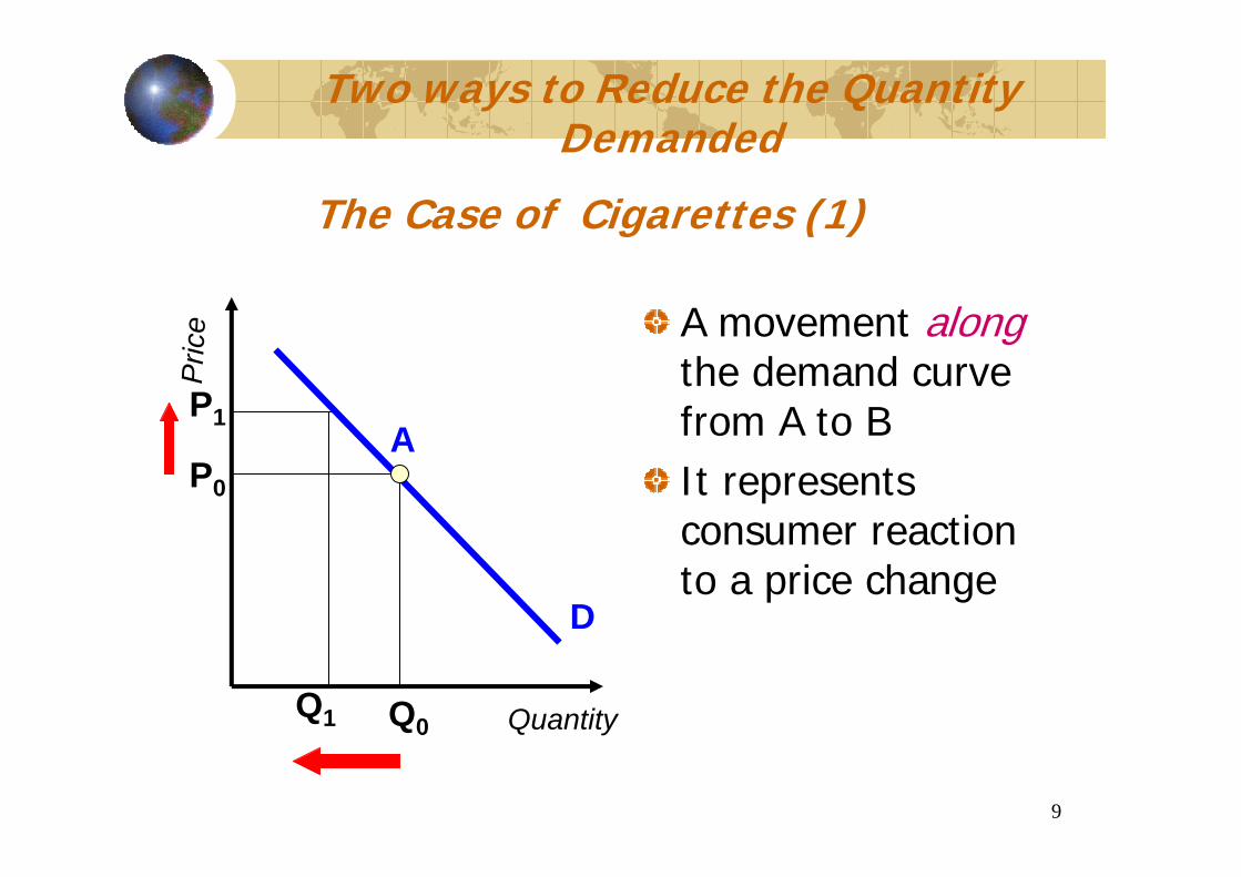
Two ways to Reduce the Quantity Demanded

A movement alongthe demand curve from A to BIt represents consumer reaction to a price change

AP0

Q0 Quantity

Pric

e

D

Q1

P1

The Case of Cigarettes (1)

10

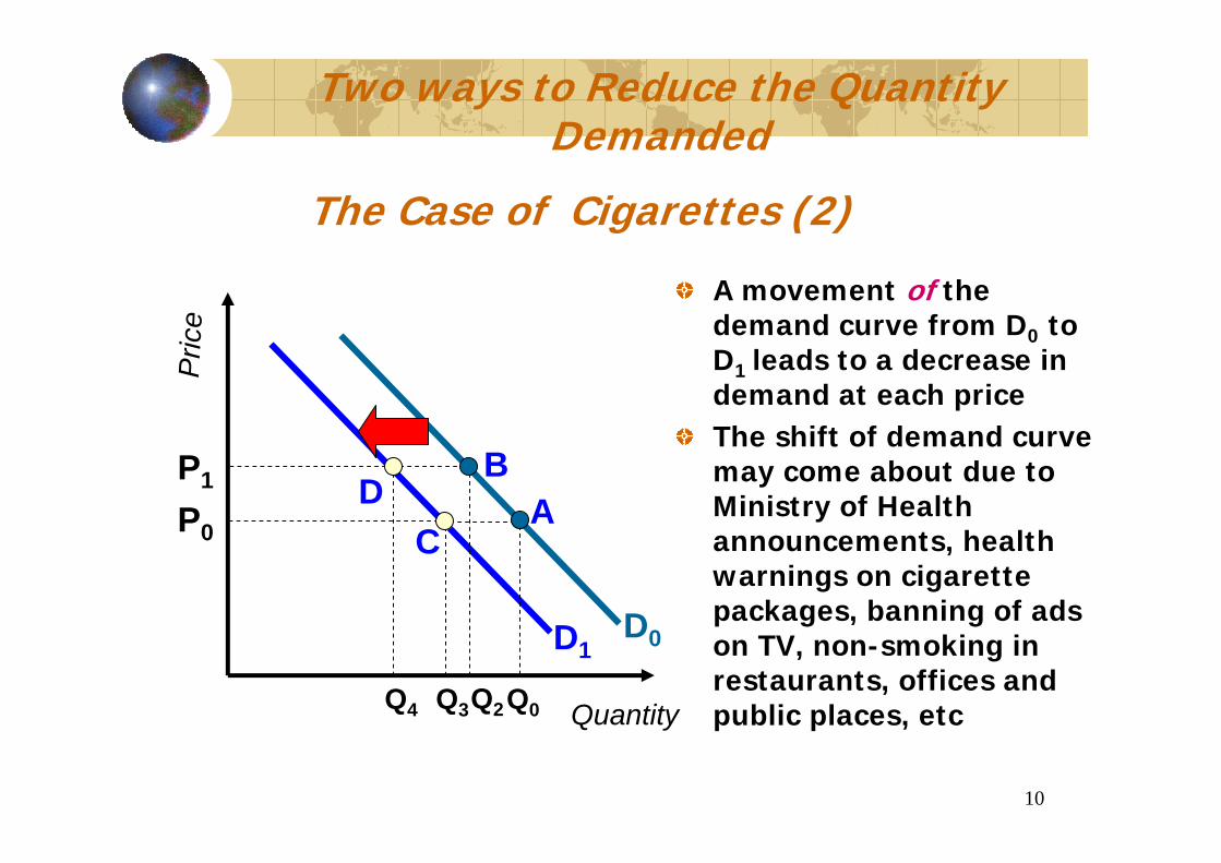
A movement of the demand curve from D0 to D1 leads to a decrease in demand at each priceThe shift of demand curve may come about due to Ministry of Health announcements, health warnings on cigarette packages, banning of ads on TV, non-smoking in restaurants, offices and public places, etc

DC

P1

Q4 Q3

D1

Quantity

Pric

e

P0

B

D0

A

Q2Q0

Two ways to Reduce the Quantity Demanded

The Case of Cigarettes (2)

11

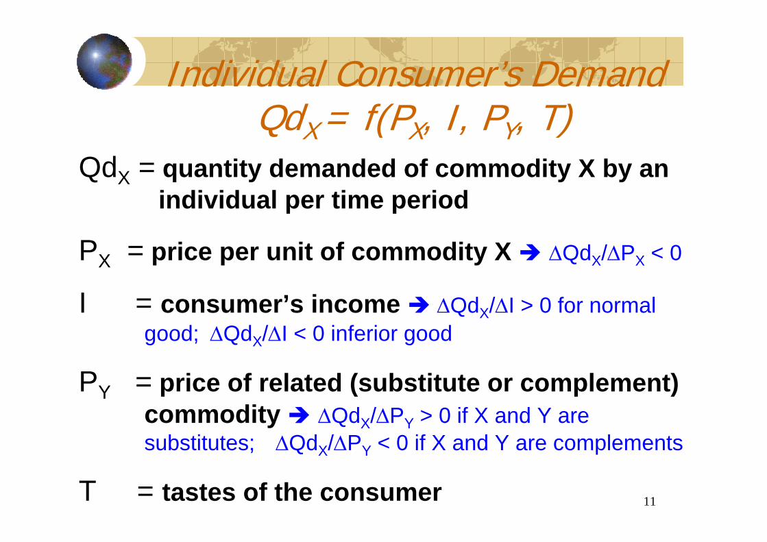
Individual Consumer’s DemandQdX = f(PX, I, PY, T)

QdX = quantity demanded of commodity X by an individual per time period

PX = price per unit of commodity X ∆QdX/∆PX < 0

I = consumer’s income ∆QdX/∆I > 0 for normal good; ∆QdX/∆I < 0 inferior good

PY = price of related (substitute or complement) commodity ∆QdX/∆PY > 0 if X and Y are substitutes; ∆QdX/∆PY < 0 if X and Y are complements

T = tastes of the consumer

12

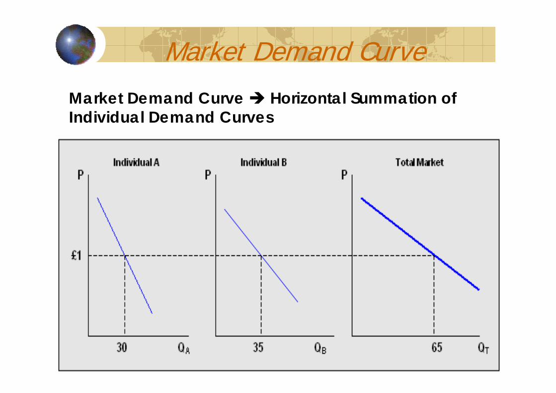
Market Demand CurveMarket Demand Curve Horizontal Summation of Individual Demand Curves

13

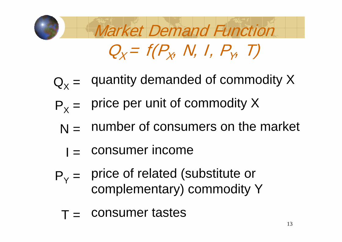
Market Demand FunctionQX = f(PX, N, I, PY, T)

quantity demanded of commodity X

price per unit of commodity X

number of consumers on the market

consumer income

price of related (substitute or complementary) commodity Y

consumer tastes

QX =

PX =

N =

I =

PY =

T =

14

Market Demand Function --An Example

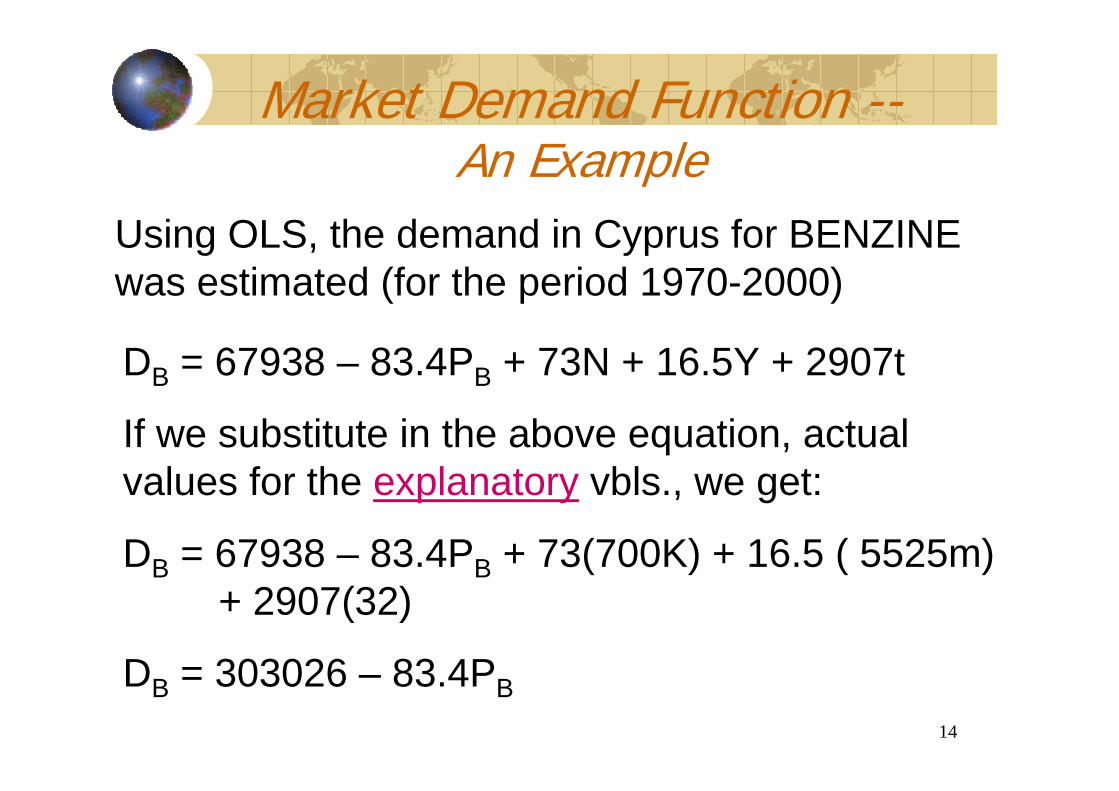
DB = 67938 – 83.4PB + 73N + 16.5Y + 2907t

If we substitute in the above equation, actual values for the explanatory vbls., we get:

DB = 67938 – 83.4PB + 73(700K) + 16.5 ( 5525m) + 2907(32)

DB = 303026 – 83.4PB

Using OLS, the demand in Cyprus for BENZINE was estimated (for the period 1970-2000)

15

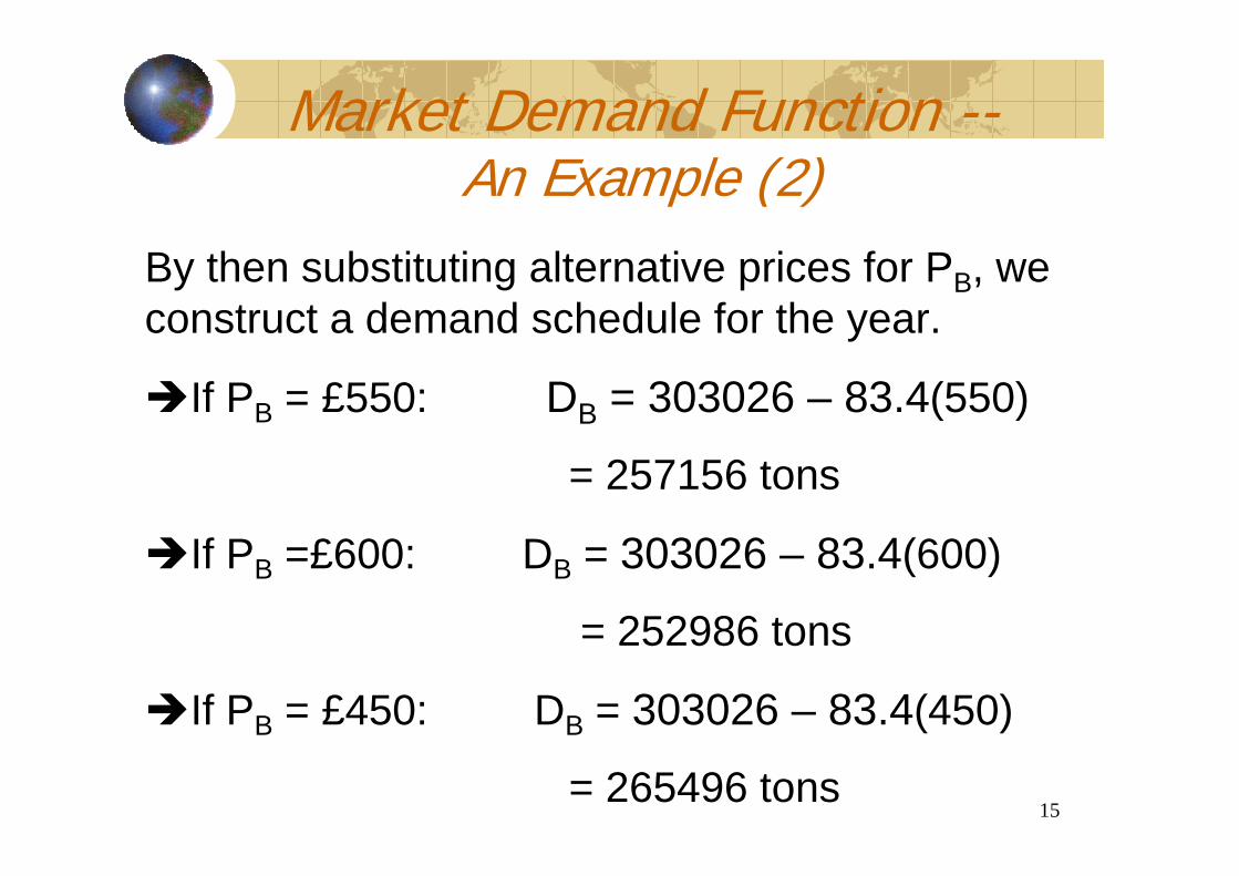
By then substituting alternative prices for PB, we construct a demand schedule for the year.

If PB = £550: DB = 303026 – 83.4(550)

= 257156 tons

If PB =£600: DB = 303026 – 83.4(600)

= 252986 tons

If PB = £450: DB = 303026 – 83.4(450)

= 265496 tons

Market Demand Function --An Example (2)

16

The Market Demand Curve (3)

Quantity

Price of Benzine

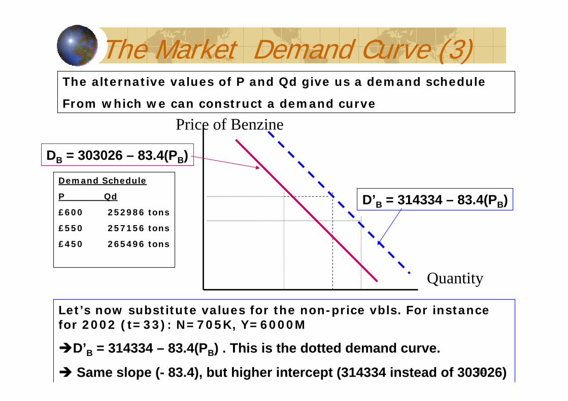
Demand Schedule

P Qd

£600 252986 tons

£550 257156 tons

£450 265496 tons

The alternative values of P and Qd give us a demand schedule

From which we can construct a demand curve

Let’s now substitute values for the non-price vbls. For instance for 2002 (t=33): N=705K, Y=6000M

D’B = 314334 – 83.4(PB) . This is the dotted demand curve.

Same slope (- 83.4), but higher intercept (314334 instead of 303026)

DB = 303026 – 83.4(PB)

D’B = 314334 – 83.4(PB)

17

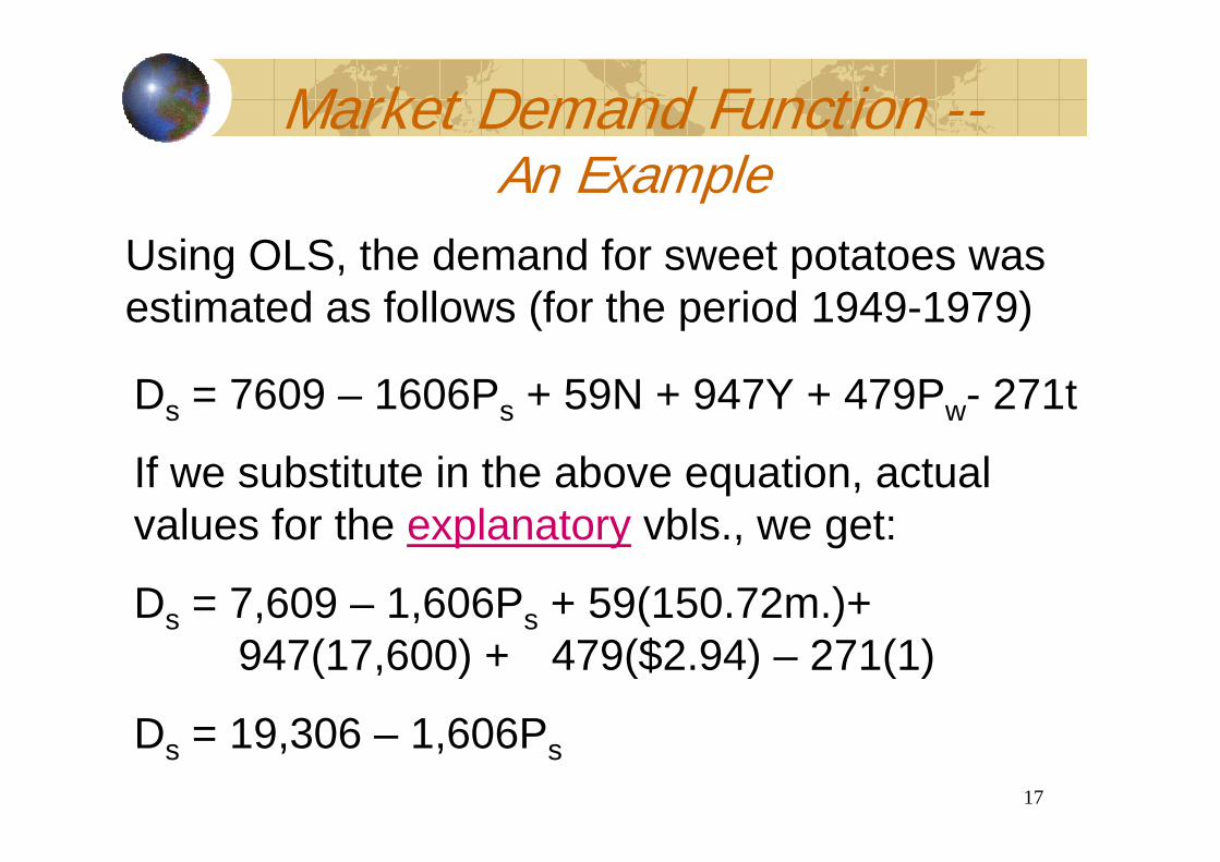
Market Demand Function --An Example

Ds = 7609 – 1606Ps + 59N + 947Y + 479Pw- 271t

If we substitute in the above equation, actual values for the explanatory vbls., we get:

Ds = 7,609 – 1,606Ps + 59(150.72m.)+ 947(17,600) + 479($2.94) – 271(1)

Ds = 19,306 – 1,606Ps

Using OLS, the demand for sweet potatoes was estimated as follows (for the period 1949-1979)

18

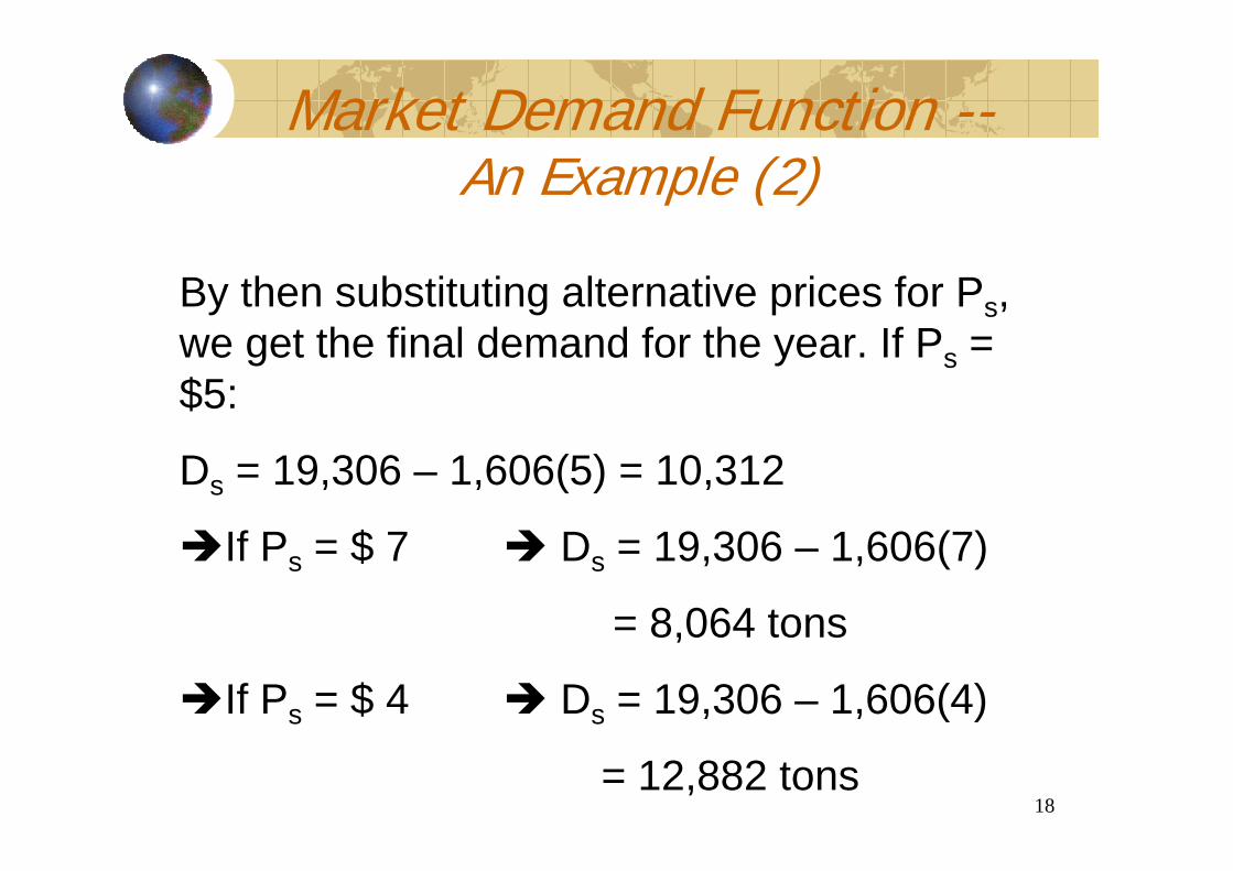
By then substituting alternative prices for Ps, we get the final demand for the year. If Ps = $5:

Ds = 19,306 – 1,606(5) = 10,312

If Ps = $ 7 Ds = 19,306 – 1,606(7)

= 8,064 tons

If Ps = $ 4 Ds = 19,306 – 1,606(4)

= 12,882 tons

Market Demand Function --An Example (2)

19

The Supply Curve

20

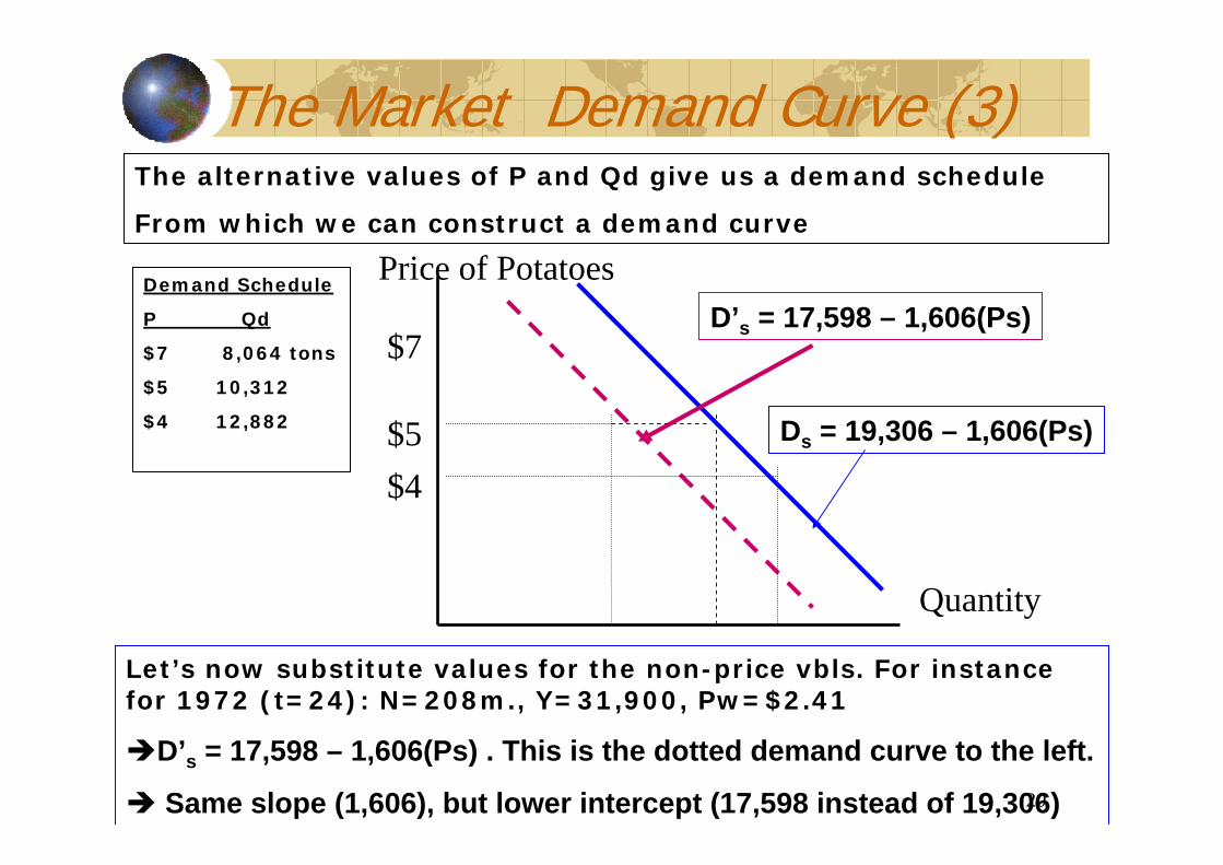
The Market Demand Curve (3)

Quantity

Price of Potatoes

$4$5

Demand Schedule

P Qd

$7 8,064 tons

$5 10,312

$4 12,882

The alternative values of P and Qd give us a demand schedule

From which we can construct a demand curve

Let’s now substitute values for the non-price vbls. For instance for 1972 (t=24): N=208m., Y=31,900, Pw=$2.41

D’s = 17,598 – 1,606(Ps) . This is the dotted demand curve to the left.

Same slope (1,606), but lower intercept (17,598 instead of 19,306)

D’s = 17,598 – 1,606(Ps)

Ds = 19,306 – 1,606(Ps)

$7

21

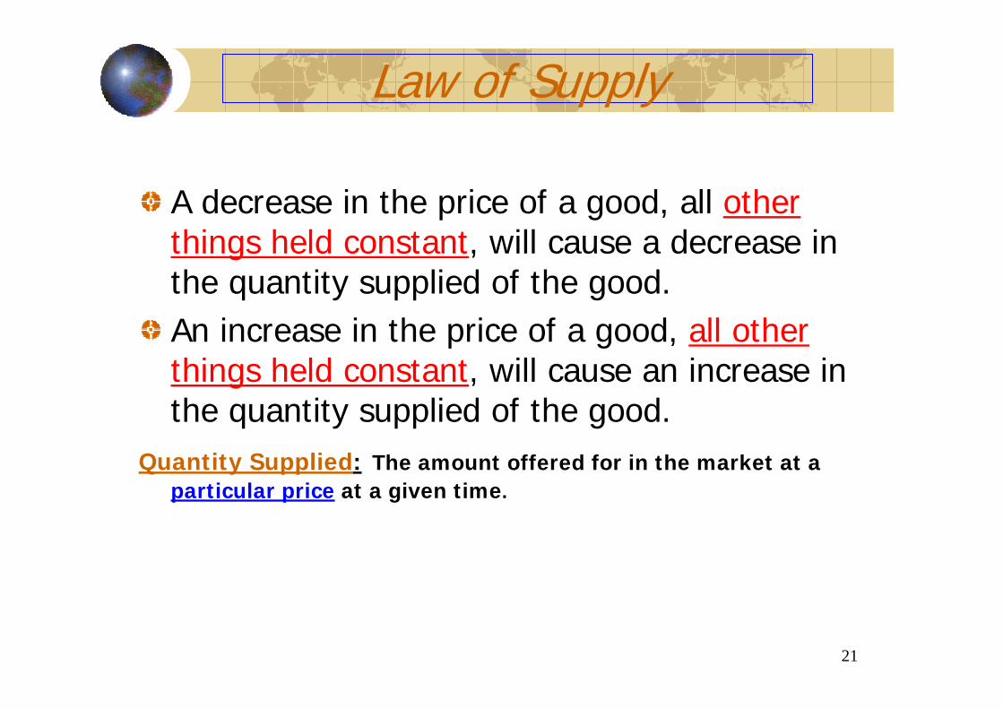
Law of Supply

A decrease in the price of a good, all other things held constant, will cause a decrease in the quantity supplied of the good.An increase in the price of a good, all other things held constant, will cause an increase in the quantity supplied of the good.

Quantity Supplied: The amount offered for in the market at a particular price at a given time.

22

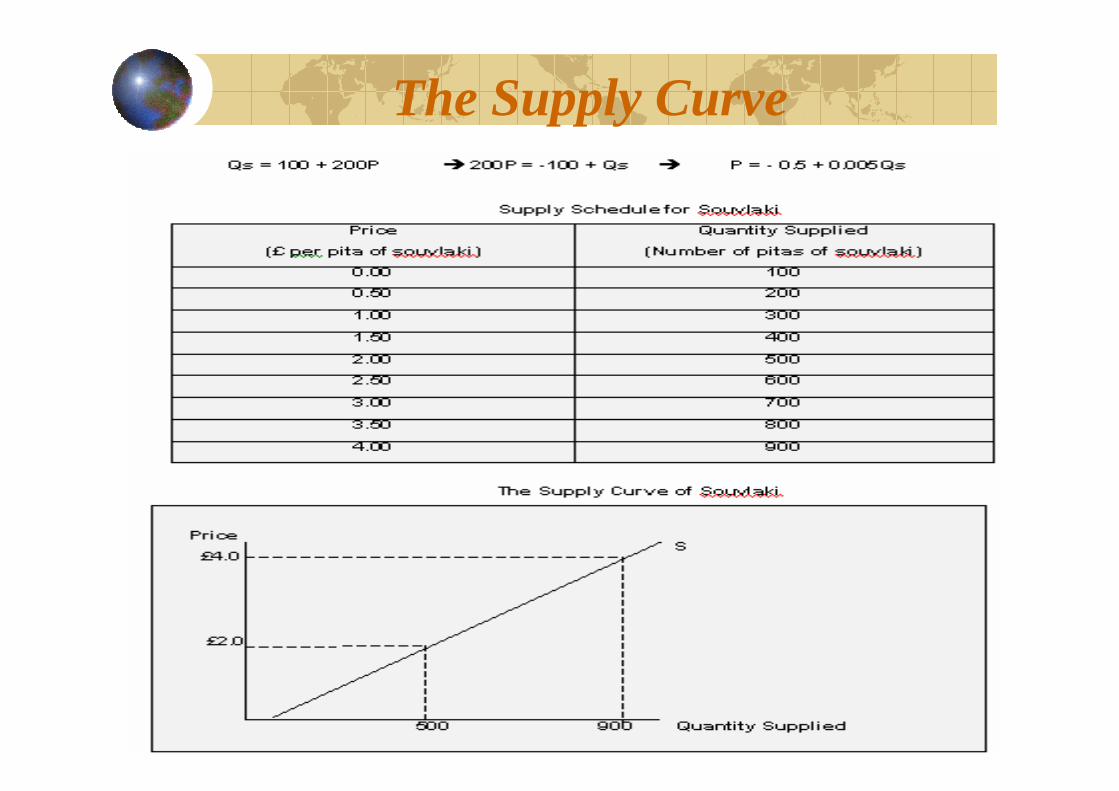
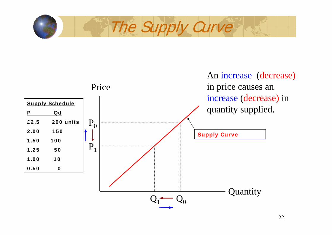
The Supply Curve

Quantity

Price

P1

Q1

P0

Q0

An increase (decrease)in price causes an increase (decrease) in quantity supplied.

Supply Curve

Supply Schedule

P Qd

£2.5 200 units

2.00 150

1.50 100

1.25 50

1.00 10

0.50 0

23

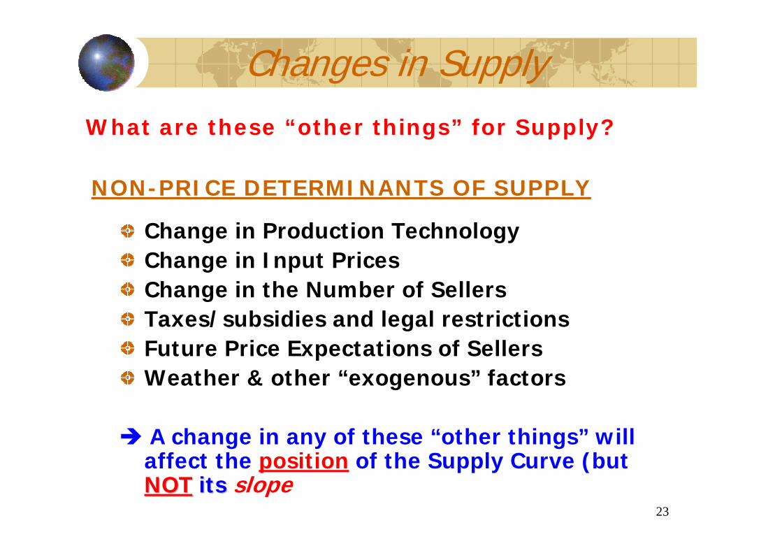
Changes in Supply

Change in Production TechnologyChange in Input PricesChange in the Number of SellersTaxes/subsidies and legal restrictionsFuture Price Expectations of SellersWeather & other “exogenous” factors

A change in any of these “other things” will affect the position of the Supply Curve (but NOTNOT itsits slope

What are these “other things” for Supply?

NON-PRICE DETERMINANTS OF SUPPLY

24

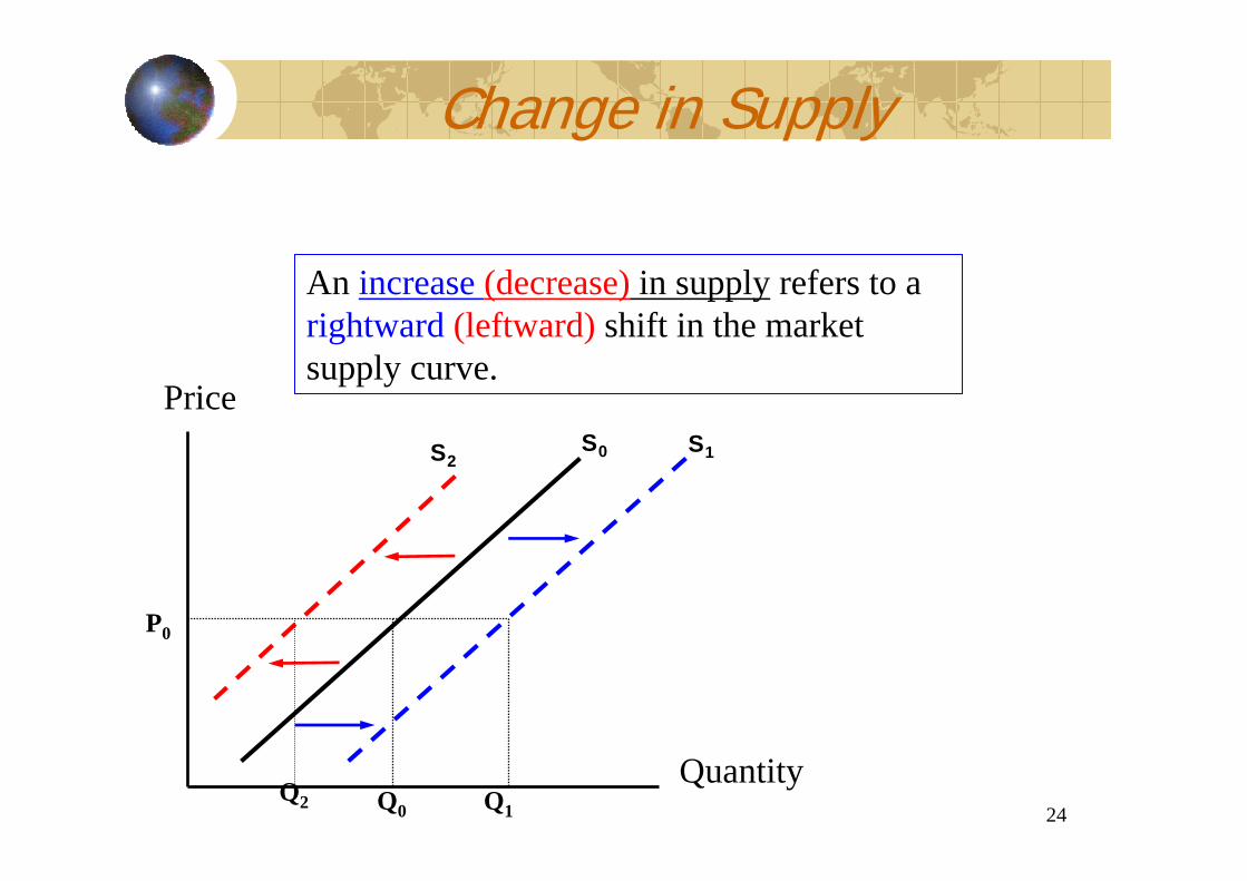
Change in Supply

Quantity

Price

P0

Q1Q0

An increase (decrease) in supply refers to a rightward (leftward) shift in the market supply curve.

S0S2S1

Q2

25

Market Equilibrium

Equilibrium: A position of balance, from which there are no inherent forces or tendencies to move away.Market equilibrium is determined at the intersection of the market demand curve and the market supply curve.Equilibrium price: The price at which the quantity demanded is equal to the quantity supplied; there is no surplus (excess supply), nor shortage (excess demand)

26

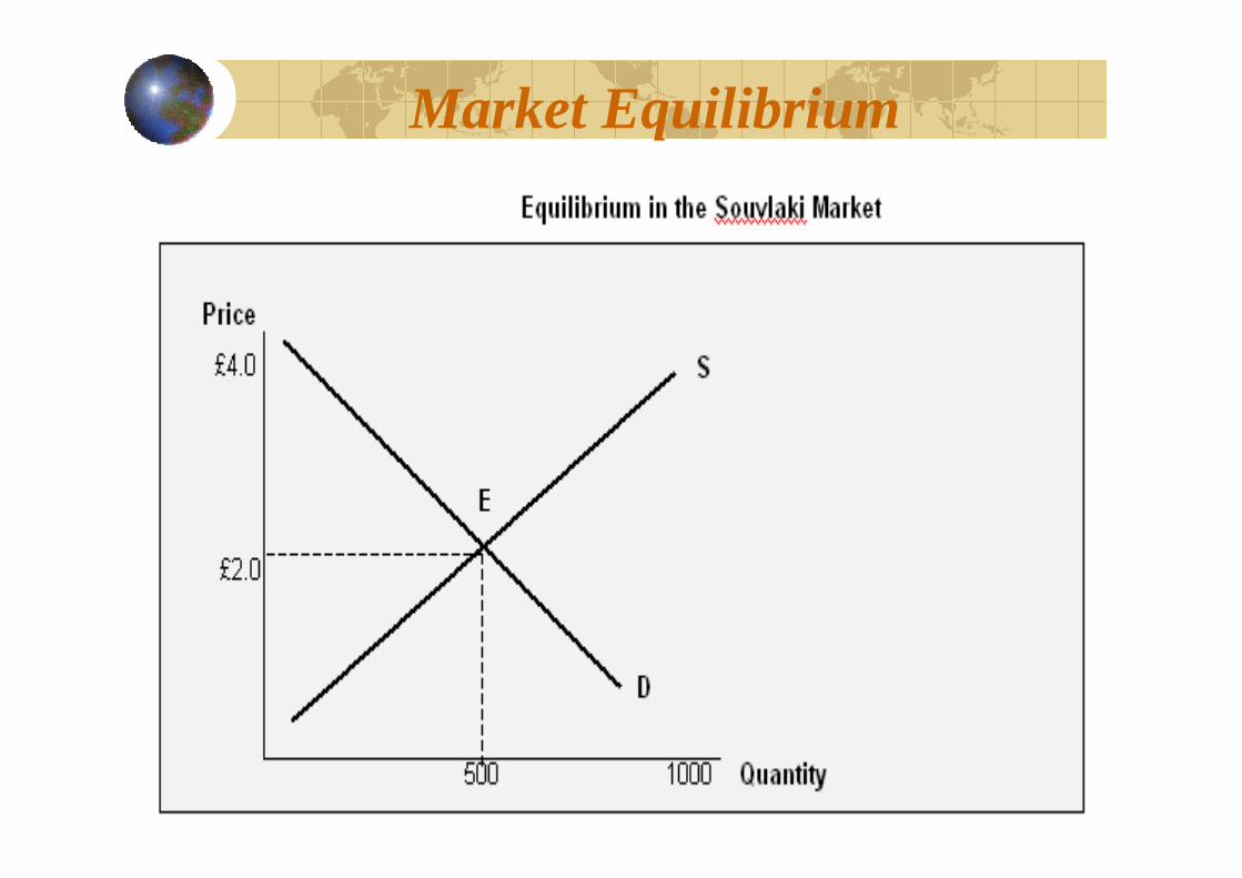
Market Equilibrium

27

Quantity

Price

Po

Qo

D S

E

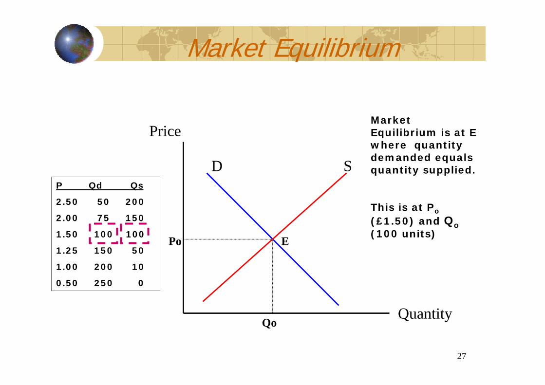
P Qd Qs

2.50 50 200

2.00 75 150

1.50 100 100

1.25 150 50

1.00 200 10

0.50 250 0

Market Equilibrium is at E where quantity demanded equals quantity supplied.

This is at Po

(£1.50) and Qo(100 units)

Market Equilibrium

28

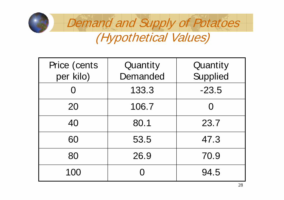
Demand and Supply of Potatoes(Hypothetical Values)

100

80

60

40

20

0

Price (cents per kilo)

0

26.9

53.5

80.1

106.7

133.3

Quantity Demanded

94.5

70.9

47.3

23.7

0

-23.5

Quantity Supplied

29

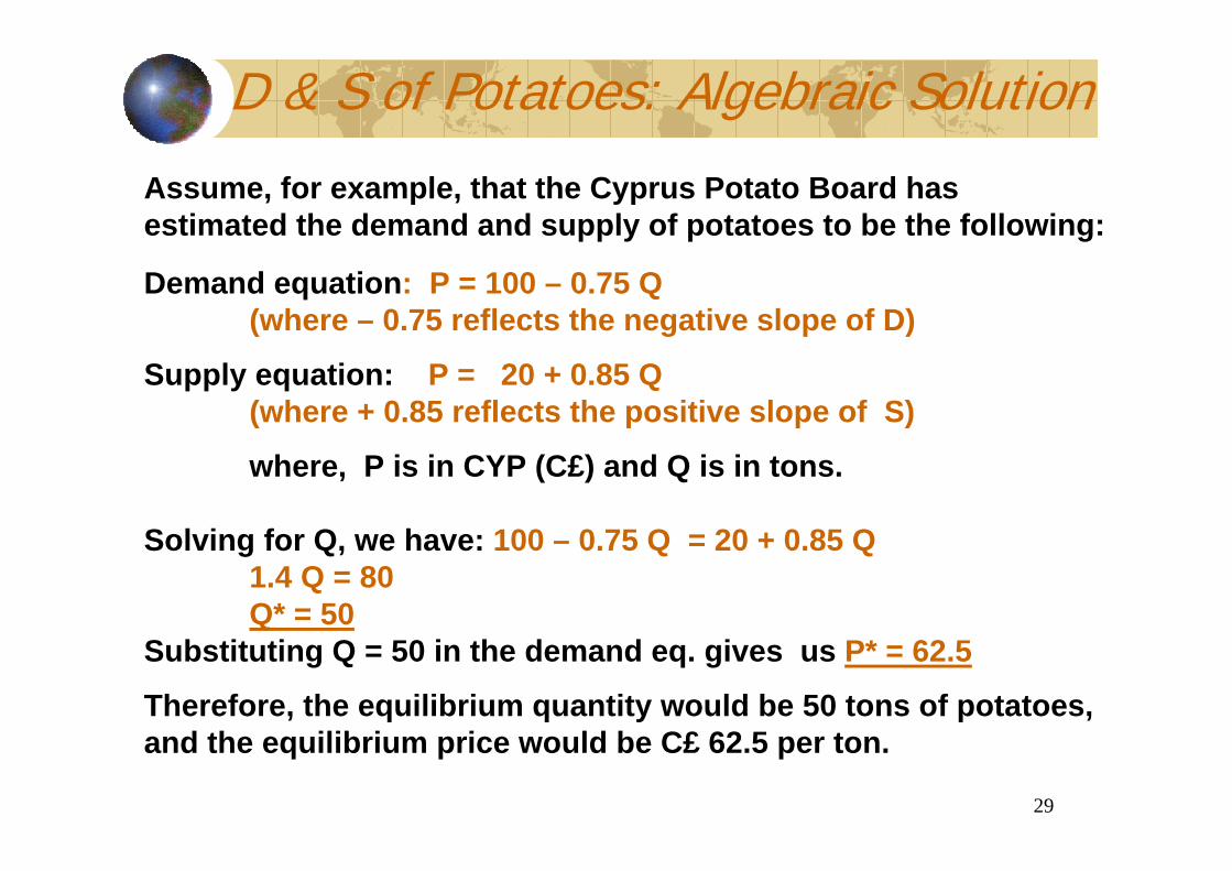
Assume, for example, that the Cyprus Potato Board has estimated the demand and supply of potatoes to be the following:

Demand equation: P = 100 – 0.75 Q(where – 0.75 reflects the negative slope of D)

Supply equation: P = 20 + 0.85 Q(where + 0.85 reflects the positive slope of S)

where, P is in CYP (C£) and Q is in tons.

Solving for Q, we have: 100 – 0.75 Q = 20 + 0.85 Q1.4 Q = 80Q* = 50

Substituting Q = 50 in the demand eq. gives us P* = 62.5

Therefore, the equilibrium quantity would be 50 tons of potatoes, and the equilibrium price would be C£ 62.5 per ton.

D & S of Potatoes: Algebraic Solution

30

Market Equilibrium and Disequilibrium

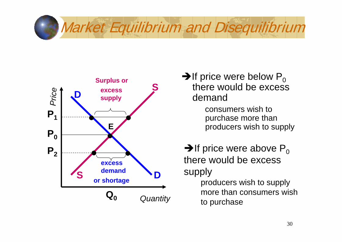
If price were below P0there would be excess demand

consumers wish to purchase more than producers wish to supply

D

DS

S

Q0

P0E

Pric

e

Quantity

•

P1 ••

excess supply

P2 • •excess demand

If price were above P0there would be excess supply

producers wish to supply more than consumers wish to purchase

Surplus or

or shortage

31

A Shift in Demand (1)

S

S

E1

Pr ic

e

Quantity

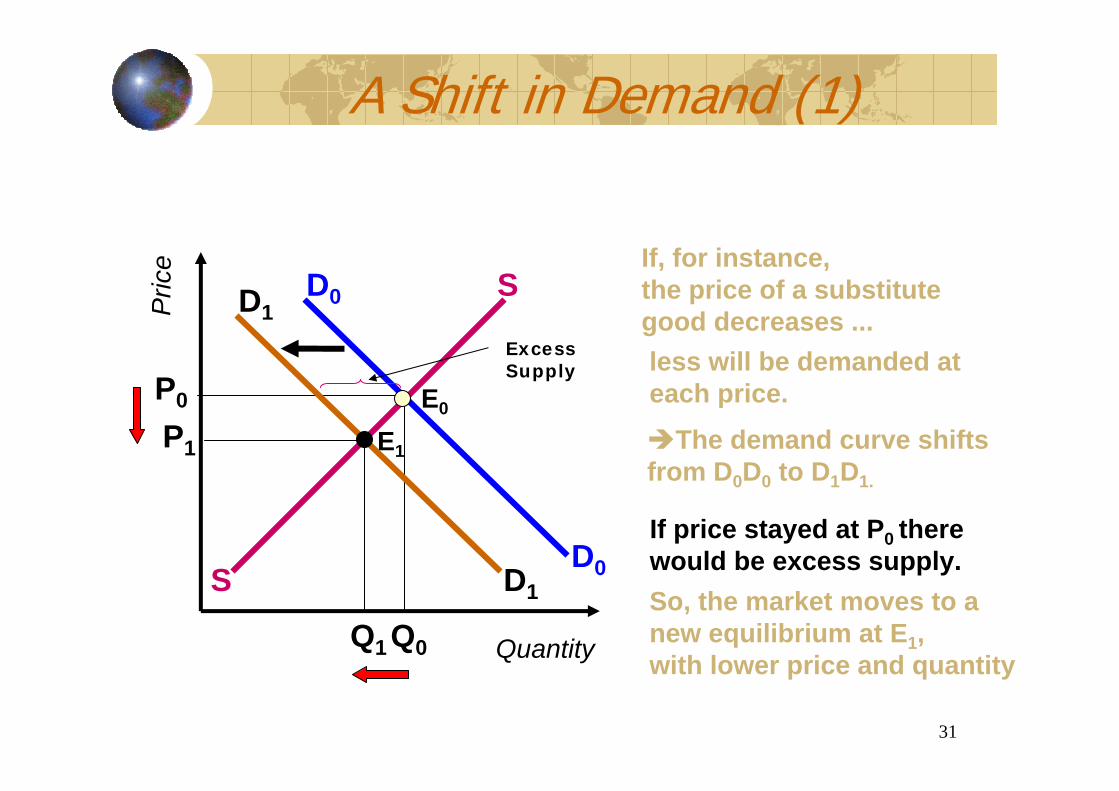
If, for instance, the price of a substitute good decreases ...less will be demanded ateach price.

D0

D0

E0

Q0

P0

The demand curve shiftsfrom D0D0 to D1D1.

D1

D1

Q1

P1

So, the market moves to a new equilibrium at E1, with lower price and quantity

If price stayed at P0 there would be excess supply.

Excess Supply

32

Quantity

Price

P0

Q0

D0 S0

Q1

P1

D1

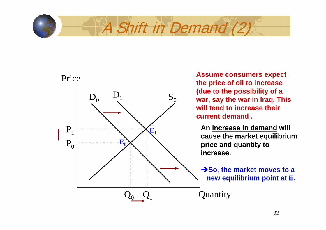
An increase in demand will cause the market equilibrium price and quantity to increase.

So, the market moves to a new equilibrium point at E1

Assume consumers expect the price of oil to increase (due to the possibility of a war, say the war in Iraq. This will tend to increase their current demand .

E1

E0

A Shift in Demand (2)

33

D

D

Q0

P0 E0

Pric

e

Quantity

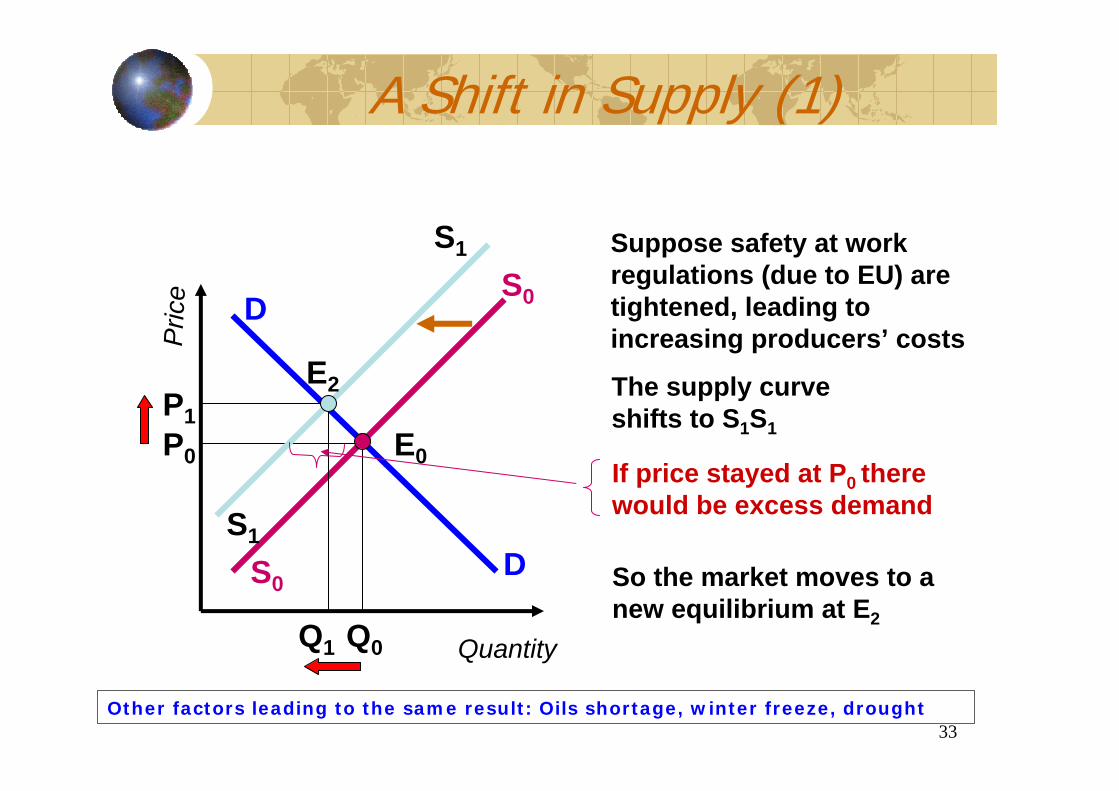
Suppose safety at workregulations (due to EU) are tightened, leading toincreasing producers’ costs

S0

S0

S1

S1

The supply curve shifts to S1S1

If price stayed at P0 there would be excess demand

Q1

P1

E2

So the market moves to a new equilibrium at E2

Other factors leading to the same result: Oils shortage, winter freeze, drought

A Shift in Supply (1)

34

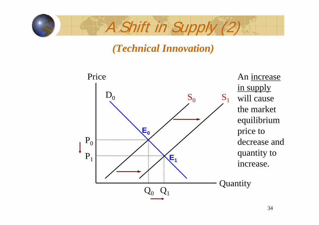
(Technical Innovation)

Quantity

Price

P0

Q0

D0 S0

Q1

P1

An increase in supplywill cause the market equilibrium price to decrease and quantity to increase.

S1

E0

E1

A Shift in Supply (2)

35

A Market in Disequilibrium (Price Controls)

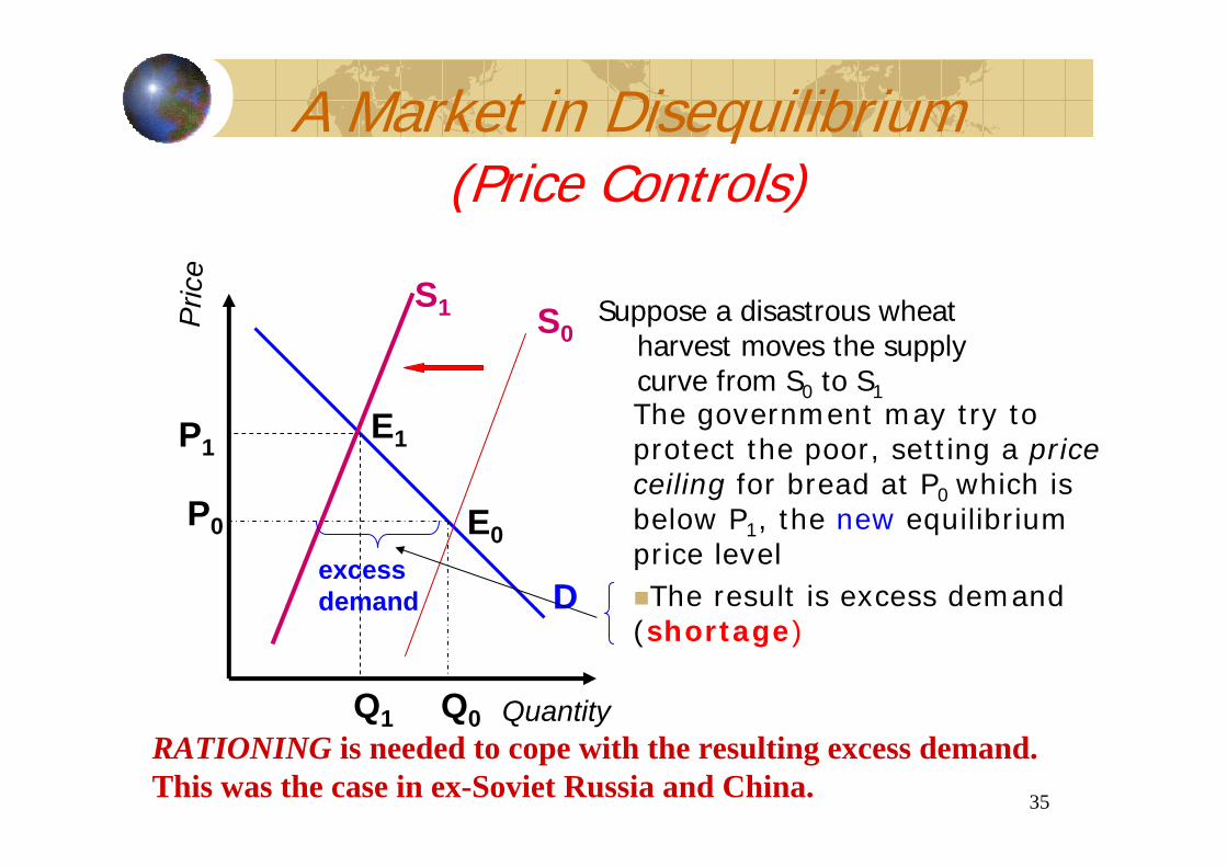
Suppose a disastrous wheat harvest moves the supply curve from S0 to S1

Quantity

Pric

e

P1

Q1

D

P0

E1

E0excess demand

Q0

S1

RATIONING is needed to cope with the resulting excess demand. This was the case in ex-Soviet Russia and China.

S0

The government may try to protect the poor, setting a price ceiling for bread at P0 which is below P1, the new equilibrium price levelThe result is excess demand

(shortage)

36

Price Supports

Quantity

Price

P0

Q0

D SSurplus

PS

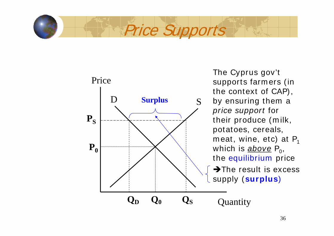
The Cyprus gov’tsupports farmers (in the context of CAP), by ensuring them a price support for their produce (milk, potatoes, cereals, meat, wine, etc) at P1 which is above P0, the equilibrium price

The result is excess supply (surplus)

QSQD

37

Price and Quantity Changes

In practice, we cannot plot ex ante demand curves and supply curvesSo,historical data and the supposition that the observed values are equilibrium ones are usedSince other things are often not constant, some detective work is required this is where our theory comes in useful

38

Demand Faced by a Firm

Market StructureMonopolyOligopolyMonopolistic CompetitionPerfect Competition

Type of GoodDurable GoodsNondurable GoodsProducers’ Goods - Derived Demand

39

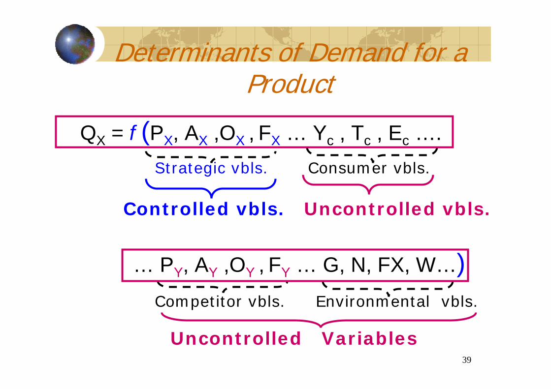
Determinants of Demand for a Product

QX = f (PX, AX ,OX , FX … Yc , Tc , Ec ….

… PY, AY ,OY , FY … G, N, FX, W…)

Strategic vbls.

Competitor vbls.

Consumer vbls.

Environmental vbls.

Uncontrolled Variables

Controlled vbls. Uncontrolled vbls.

40

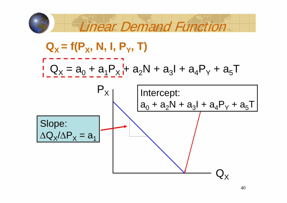
Linear Demand Function

QX = a0 + a1PX + a2N + a3I + a4PY + a5T

PX

QX

Intercept:a0 + a2N + a3I + a4PY + a5T

Slope:∆QX/∆PX = a1

QX = f(PX, N, I, PY, T)