1

DELTA-V AS A MEASURE OF TRAFFIC CONFLICT SEVERITY

Steven G. Shelby Senior Research Engineer, Econolite Control Products, Inc.,

Tucson, AZ, USA, e-mail: sshelby@econolite.com

Submitted to the 3rd

International Conference on Road Safety and Simulation,

September 14-16, 2011, Indianapolis, USA

ABSTRACT

Delta-V (∆v) is a measure of the severity of a traffic collision, defined as the change in velocity between pre-collision and post-collision trajectories of a vehicle. Delta-V emerged in the 1970s in the context of crash reconstruction analysis, and is considered by some researchers to be the best single predictor of crash severity. However, this indicator has not been applied to the analysis of traffic conflicts, until recently when it was incorporated into the automated conflict analysis algorithms of the Surrogate Safety Assessment Model (SSAM). This paper introduces Delta-V and demonstrates how it overcomes shortcomings present in several traditional measures of traffic conflict severity. We discuss the ambiguity present in the literature on the topic of traffic conflict severity, and suggest the adoption of alternative terminology and definitions. We demonstrate a new approach, incorporating Delta-V, to estimate the collision propensity and potential collision severity of a traffic conflict. Keywords: traffic, safety, conflicts, surrogate measures, delta-v, severity, collision propensity, comprehensive economic costs.

INTRODUCTION

Delta-V (∆v) is commonplace notation used in mathematics and particularly in physics to denote a change or difference in velocity. In the context of a motor vehicle crash, ∆v specifically refers to the change in velocity between pre-collision and post-collision trajectories of a vehicle.

beforeafter vvv −=∆

Delta-V emerged in the 1970s in the context of crash reconstruction analysis, and is considered by some researchers to be the best single predictor of crash severity. However, this indicator has not been applied to the analysis of traffic conflicts, until recently when it was incorporated by the author into the automated conflict analysis algorithms of the Surrogate Safety Assessment Model (SSAM).(1) Traffic conflict studies have historically been conducted with a team of observers trained to identify and characterize the severity of narrowly-averted traffic collisions as they watch traffic from the roadside. However, with the emergence of algorithmic software to

2

conduct this task, much more sophisticated measures of safety, such as ∆v, can be calculated. We note that our estimation of ∆v in the SSAM software was an overly crude first effort, but nonetheless a valuable first step toward the ideas outlined herein. We continue the introduction of ∆v in the next (second) section, and then in the third section show this single value can be used to estimate the full range of collision outcomes across the severity spectrum. However, a constructive discussion of conflict severity measures requires a common understanding of what exactly is the severity of a traffic conflict. We find the literature ambiguous and conflicting in this regard, and thus devote the third section to defining new terminology and clarifying the concept. The fourth section contrasts ∆v with traditional severity measures, illustrating its advantages, and demonstrates how to estimate ∆v in the context of a traffic conflict. The final sections show how the ∆v severity profile lends itself to the aggregation and comparison of conflicts, using comprehensive economic costs to weigh the risks. The paper is written assuming that readers are already familiar with traffic conflict techniques. However, for the benefit of unfamiliar readers, we provide a very concise synopsis and suggest reviewing a brochure describing the Swedish Traffic Conflicts Technique for a quick overview, or the recent dissertation by Archer for more comprehensive coverage.(2, 3) DELTA-V

The utility of ∆v for characterizing collision severity emerged in the 1970s, in the context of crash reconstruction analysis. The National Highway Traffic Safety Administration (NHTSA) commissioned development of a crash reconstruction program called CRASH (Calspan Reconstruction of Accident Speeds on Highways).(4, 5) This program is used to estimate the Delta-V of vehicles involved in a crash based on measurements of their structural deformation.(6) The original version of CRASH was able to estimate vehicle impact velocities to within about 12% of actual velocities. We present a simplistic equation for ∆v as follows. Suppose that vehicle 1 with mass m1 is traveling at a pre-collision velocity v1 and is encroaching on vehicle 2, a slower moving vehicle with mass m2 and pre-collision velocity v2. The post-collision velocities are marked with an overlaid tilde (~). Then, ∆v for each vehicle is simply the change between the pre-collision velocity and the post-collision velocity, as written in Equation 1.

(1)

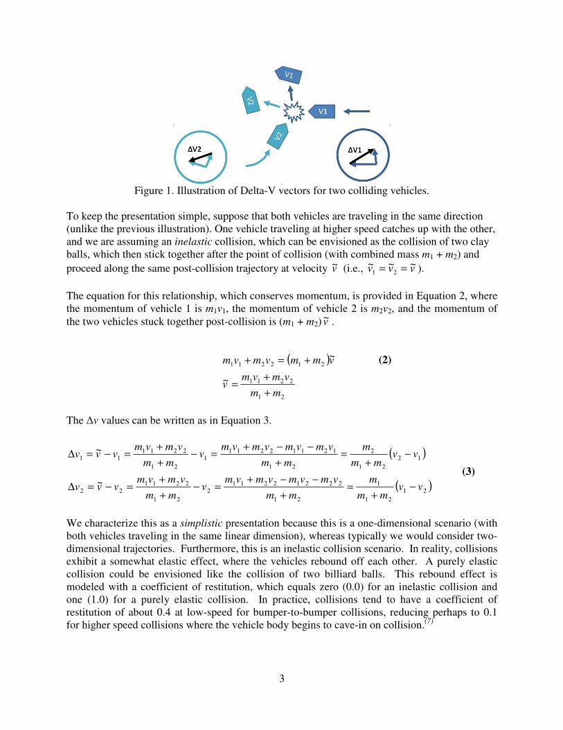
Figure 1 below illustrates two converging vehicles to an ultimate collision (the “splat” shape draw in the middle), and their post-collision trajectories (emanating from the splat), in order to visualize the notion of ∆v.

222

111

~

~

vvv

vvv

−=∆

−=∆

3

Figure 1. Illustration of Delta-V vectors for two colliding vehicles.

To keep the presentation simple, suppose that both vehicles are traveling in the same direction (unlike the previous illustration). One vehicle traveling at higher speed catches up with the other, and we are assuming an inelastic collision, which can be envisioned as the collision of two clay balls, which then stick together after the point of collision (with combined mass m1 + m2) and proceed along the same post-collision trajectory at velocity v~ (i.e., vvv ~~~

21 == ). The equation for this relationship, which conserves momentum, is provided in Equation 2, where the momentum of vehicle 1 is m1v1, the momentum of vehicle 2 is m2v2, and the momentum of the two vehicles stuck together post-collision is (m1 + m2) v~ .

(2)

The ∆v values can be written as in Equation 3.

(3)

We characterize this as a simplistic presentation because this is a one-dimensional scenario (with both vehicles traveling in the same linear dimension), whereas typically we would consider two-dimensional trajectories. Furthermore, this is an inelastic collision scenario. In reality, collisions exhibit a somewhat elastic effect, where the vehicles rebound off each other. A purely elastic collision could be envisioned like the collision of two billiard balls. This rebound effect is modeled with a coefficient of restitution, which equals zero (0.0) for an inelastic collision and one (1.0) for a purely elastic collision. In practice, collisions tend to have a coefficient of restitution of about 0.4 at low-speed for bumper-to-bumper collisions, reducing perhaps to 0.1 for higher speed collisions where the vehicle body begins to cave-in on collision.(7)

( )

21

2211

212211

~

~

mm

vmvmv

vmmvmvm

+

+=

+=+

( )

( )2121

1

21

222122112

21

221122

1221

2

21

121122111

21

221111

~

~

vvmm

m

mm

vmvmvmvmv

mm

vmvmvvv

vvmm

m

mm

vmvmvmvmv

mm

vmvmvvv

−+

=+

−−+=−

+

+=−=∆

−+

=+

−−+=−

+

+=−=∆

4

We note that the original CRASH program assumed an inelastic collision. This was later identified as a reason for underestimating ∆v values by 10% to 30%, and a subsequent version of the CRASH software was updated to account for the coefficient of restitution, which was then said to estimate initial impact velocities within about 1% of their true value.(8) This gives a feel for the ramifications of making the simplifying assumption of an inelastic collision. We will assume inelastic collisions for the calculations in this paper, as our focus is on introducing the basic concept to a new field of application, and not burying the reader in unnecessarily complex analysis. PREDICTING INJURY OR FATALITY OUTCOMES

Researchers in the 1970s were developing models to predict the likelihood that a crash would result in injuries or fatalities based on variables such as impact speed and vehicle mass, and began exploring the use of ∆v to predict injuries and fatalities.(9) It became evident that ∆v was a strong predictor of crash severity. One of the earliest efforts in 1977 explored the relationship between (a) the ∆v values estimated from the crash analysis of 173 side-impacted vehicles and (b) the mean injury severity of their corresponding occupants, rated using a measure referred to as the Abbreviated Injury Scale (AIS).(9) A least squares linear regression of this relationship yielded an R2 value of 0.86. However, perhaps the most well known result is by Joksch, who presented an approximate model he characterized as a “rule of thumb”, as shown in Equation 4, stating that mean rate or percentage (P) of two-vehicle collisions resulting in a fatality is approximately proportional to ∆v to the fourth power, based on his efforts to fit a model to crash data from the National Crash Severity Study (NCSS).(10)

(4)

Other more complex functional forms have also been considered, but additional studies have confirmed that Joksch’s rule provides a very good approximate fit. For example, O’Day and Flora found a similar power function of ∆v based on analysis of 10,000 crashes in the NCSS database from 1970 to 1979. Also, Evans analyzed over 14,000 crashes from the NCSS database from the years 1982 to 1991, and fit the generalized functional form in Equation 5 to data for both injury prediction and fatality prediction, conditioned on whether occupants wore seat belts or not.

(5)

The result of Evans effort to fit this model to crash data is illustrated in Figure 2. These equations, as drawn, are referenced later in the paper, and thus we will work with U.S. customary units to avoid conversions for this original figure from Evans. We note that all of these models were also based on the assumption of inelastic collision dynamics, and simply used the scalar value (magnitude) of ∆v.

4

71

∆=

vP

kv

P

∆=

α

5

Figure 2. Illustration of actual crash outcomes to predicted outcomes. (Source: Evans, 1994)

Researchers over the years have stated great confidence in ∆v as an indicator of crash severity with statements such as the following:

•••• “Empirical data show unequivocally that injuries and fatality rates increase as a power function of impact speed or Delta-V.”(11)

•••• “It is well known that the ∆v is the best single predictor of injury and fatality risk in a crash.”(12)

•••• “[Delta-V] is the best available measure of crash severity for vehicles that have not been specially instrumented for crash testing.”(13)

SEVERITY

Notions regarding the severity of an actual crash are fairly well-established; however, the concept of severity is much more ambiguous in the context of traffic conflict literature. This section reviews these two seemingly incongruent perspectives and we suggest specific terminology and interpretations with the aim of clarifying future discussion. When speaking of motor vehicle crashes, severity is defined in terms of the magnitude of adverse consequences, which for the most part could be characterized as damages, to both property and health. Crashes are typically classified as a fatality crash, an injury crash, or a property-damage-only (PDO) crash based on the severity of the worst injury amongst all people involved in the

6

crash. However, in the context of traffic conflicts, the notion of severity often takes a different character. Perhaps this alternative perspective arises from the reality that outcomes in terms of bodily harm and property damage are not directly measurable in a narrowly-averted crash scenario. It is more natural to say, “That was a close one.” Indeed, the literature on traffic conflict severity tends to utilize terms such as nearness, closeness, or proximity to express severity. Conflicts are also commonly characterized as “serious” or “severe” when a more or less arbitrary severity threshold has been exceeded. Notions of traffic conflict severity that appear in the literature can generally be classified into one of the following four camps:

•••• Severity is the probability of crashing. •••• Severity is the magnitude of the damages from a potential collision. •••• Severity is both of the above. •••• Severity is equated to a quantitative value, with no explicitly defined interpretation.

The following subsections present examples of the term “severity” used in each of the senses. Severity as a probability of crashing

Gettman and Head have said, “The sizes of the surrogates TTC, PET, and DR indicate the severity of the conflict event, that is, the probability that a collision could result from a conflict, such that a lower TTC indicates a higher probability of a collision, a lower PET indicates a higher probability of a collision, and a higher DR indicates a higher probability of a collision.”(14) Likewise, Saunier et al. model a conflict collision probability as an exponential function of a time-to-collision estimate, saying, “The collision probability can be considered as the normalized severity dimension of the safety hierarchy.”(15) Severity as the magnitude of damages from a potential collision

Gettman and Head state, “It is important to distinguish both the severity of the conflict and the severity of the resulting collision.” Whereas their definition of the severity of a conflict was based on the probability that a conflict would result in a collision, they suggest other indicators for the resulting collision severity as follows. “MaxS and DeltaS are used to indicate the likely severity of the (potential) resulting collision if the conflict event had resulted in a collision instead of a near miss.”(14) Svensson suggests, “The severity should be related to the probability of serious injury.”(16) Svennson says this while discussing the Swedish Traffic Conflicts Technique and its corresponding severity indicator, given by a ratio of the Time-to-Accident (TA) to the Conflicting Speed (CS). These terms are defined as follows:

•••• Time-to-Accident (TA) is “the time that remains to an accident from the moment that one of the road users starts an evasive action if they had continued with unchanged speeds and directions.”

•••• Conflicting Speed (CS) is the speed of the road user taking evasive action, for whom the TA value is estimated, at the moment just before the start of the evasive action.”

7

Figure 3 presents the notion of the uniform severity level, where the bold red curve delineates serious conflicts from non-serious conflicts. Uniform severity zones are bands of equivalent severity.

Figure 3. Bands of uniform severity levels defined by the ratio TA/CS. Source: (Archer, 2005).

Severity as both a crash probability and the magnitude of potential damages

Svennson teamed with Hyden to publish another paper on the topic of conflict severity, wherein the same measure of severity, TA/CS, is characterized differently as follows. “The aim must, furthermore, be to construct a severity hierarchy for traffic events so that for each event a severity, i.e. the event’s closeness to a crash, can be estimated.”(17) While this description suggests the probability that a conflict results in a crash, the paper goes on to say, “At this very moment we can say that an unknown event with a certain location in the severity hierarchy has a certain closeness to an injury crash, i.e. a certain probability of resulting in an injury crash.” Thus, Svensson and Hyden refer to the TA/CS indicator as providing both the probability of an unqualified crash of any type and also the probability that this crash includes an injury. “The information we get from each interaction and its severity, is how close this particular interaction was to a crash, i.e. how imminent the danger was.” Severity as an ordinal quantitative measure, with no explicit interpretation

Sayed has suggested, “The TTC value represents the conflict severity. The smaller the TTC value the more severe the conflict. Conflicts with TTC value less than 1 second are usually considered to be severe conflicts.”(18) Thus, severity has been expressed purely as a quantitative value, without any particular meaning being ascribed to the indicator. Similarly, Chin and Quek suggest the reciprocal of TTC is a measure of severity, stating, “… since time-to-collision decreases with increasing severity, it would be better to represent the conflict measure in terms

8

of the reciprocal of time-to-collision, which increases with increasing severity.”(19) They additionally suggest that the deceleration rate necessary to avoid collision “also reflects the severity of the conflict, since the higher the value of the deceleration, the more serious is the conflict.” We have shown that the notion of severity as discussed in the traffic conflict literature takes a range of ambiguous and conflicting definitions from one paper to the next, and in some cases within the same paper. We present the following terminology and definitions to bring some clarity to the nomenclature in this paper, and hopefully to future literature on this topic.

•••• Collision propensity is the probability that an emerging conflict results in a collision.

•••• Collision severity or potential collision severity is the expected magnitude of the consequences of a collision, given that a collision occurs.

•••• Conflict severity is the expected consequences of the emerging conflict event, considering

the estimated distribution of no collision and collision outcomes. We briefly discuss some of the motivation behind this nomenclature. We prefer to keep usage of the term severity in the context of traffic conflicts consistent with its usage in the context of actual crashes, where it already has a universal connation of the magnitude of resulting consequences. In the context of a traffic conflict, outcomes are not known, and thus severity takes the form of an expectation. We suggest refraining from using the term traffic conflict severity as a collision probability, since that is not consistent with notions of crash severity. We feel it is crucial to explicitly acknowledge that collision propensity and potential collision severity are two distinct dimensions in the character a traffic conflict. As we demonstrate later in this paper, two traffic conflicts with the same collision propensity may exhibit dramatically different potential collision severities. We refer to these two separate dimensions by two different names for clarity, as opposed to the confusion created and prolonged by referring to both dimensions as severity. We prefer the term propensity to the term proximity, which implies physical or temporary closeness. Propensity captures the probabilistic estimation we truly seek, whereas proximity implies relative or ordinal relations that are often not true. For example, it is commonly stated that shorter time-to-collision (i.e., temporal proximity) corresponds to a higher probability that a conflict results in a collision. However, we will show that this is not true in the following section. Similarly, two closely-spaced vehicles in conflict do not necessarily present a higher probability of collision than two vehicles with relatively distant spacing. While these notions may often be true, they are certainly not always true, whereas a higher probability of collision does, by definition, always correspond to a higher probability of collision. We also adopt the term propensity in favor of the term probability, as it seems somewhat odd to observe a traffic conflict—which does not result in an actual collision in the vast majority of cases—and then subsequently speak of that conflict’s collision probability being nonzero, when we already know

9

that it did not result in an actual collision. The notion of propensity is rather more loosely and pragmatically defined, but can be taken as the long-run relative frequency of collisions, given a sufficiently large number of replications of the same situation. This focus on the “generating conditions” is also consistent with our suggested methodology of calculating propensity based on the situation—the location and velocity of the involved vehicles—at the moment the traffic conflict emerges.

COMPARISON WITH TRADITIONAL SEVERITY MEASURES

The section compares and contrast Delta-V with several traditional measures of severity, elucidating their respective shortcomings, and thereby highlighting the overall robustness of Delta-V to a broad range of conflict scenarios. The measures have been divided into two categories of values: (a) directly measurable indicators, and (b) estimated indicators. Directly Measurable Indicators

Directly measurable indicators can be directly observed from the trajectories of two converging vehicles. They provide useful indications of relative severity in limited scenarios, but as we will show, they also fail to accurately distinguish severity when faced with a broader range of traffic conflict situations. Maximum Speed (Max S) Maximum Speed (Max S) indicates the maximum observed speed of either vehicle during a conflict event.(14) This is considered an indicator of collision severity, with the understanding that “speed kills”. Its strengths and weaknesses are illustrated by the follow cases:

•••• Case 1 – Vehicle A is traveling eastbound (EB) at a speed of 40 mph, and rear-ends vehicle B, which is stationary. The Max S value is 40 mph. Delta-V can be calculated assuming an inelastic collision, which is a collision where both vehicles stick together after the collision. This simplifying assumption is adopted throughout this paper. In this case, assuming equal mass vehicles, both vehicles would have a post-collision EB trajectory at 20 mph. Both vehicles would have a ∆v of 20 mph.

•••• Case 2 – This is the same as case 1, except vehicle A is traveling 20 mph, in which case the Max S value is 20 mph, which suggests a less severe collision. Delta-V is 10 mph in this case, for both vehicles, also indicating lower severity than Case 1.

•••• Case 3 – Vehicle A is traveling EB at 40 mph and crashes head-on into vehicle B, which

is traveling westbound (WB) at 30 mph. The Max S value for this collision is 40 mph. The post-collision trajectory of both vehicles is EB at 5 mph. The ∆v for both vehicles is 35 mph.

Max S is successful in distinguishing that Case 1 is more severe than Case 2. Note that it is possible to directly estimate the probability of an injury, and the probability of a fatality, based on ∆v, using the equations provided in Figure 2. We will assume that all vehicle occupants are

10

wearing seat belts. Note that both severity measures in Case 2 are half of their respective values in Case 1. However, the probabilities of injuries and fatalities are a power function of ∆v, and thus differences in the probability of injuries are much greater than 50% between Cases 1 and 2. The probability of injury is 0.041 in Case 1, and 0.007 in Case 2. Case 3 illustrates the shortcoming of Max S. In Case 3, the probability of an injury is 0.180, whereas the probability of an injury in Case 1 is 0.041, despite having the same Max S severity indicator. Similarly, the probability of a fatality in Case 3 is 0.044, whereas the probability of fatality in Case 1 is 0.003, despite having the same Max S severity indicator. A fundamental weakness of the Max S indicator is that speed is a scalar value, with no notion of direction of travel, whereas velocity is a vector, which has both magnitude and direction. Thus, ∆v can distinguish the extreme severity of a head-on collision from the minor severity of a rear-end collision, whereas the Max S indicator cannot. Relative Speed The measure Delta S (∆s) is the maximum difference in speeds between the two vehicles during a conflict event.(14) This is considered an indicator of collision severity, with the understanding that the higher the difference in speeds in a rear-end accident, the higher the severity. This measure suffers the same fundamental shortcoming as Max S, in considering only the magnitude of speeds and not the direction. Using the cases from the Max S discussion, ∆s is 40 mph in Case 1 and ∆s is 20 mph in Case 2. So, ∆s is successful in distinguishing that Case 1 is more severe than Case 2. However, ∆s is 10 mph in Case 3, which suggests that Case 3 is less severe than Case 2. However, using ∆v, we calculated a probability of fatality of 0.044 for Case 3, and 0.000 for Case 2. Thus, Delta S has utterly failed in this case. Post-Encroachment Time Post-encroachment time (PET) is the elapsed time between the departure of a leading vehicle and the arrival of the trailing vehicle at the same location. Consider a crossing conflict where one vehicle turns in front of an oncoming vehicle. A shorter elapsed time between the departure of the turning vehicle and the arrival of the oncoming vehicle suggests greater risk of collision. However, there are commonplace scenarios where PET does not accurately portray relative severity. Suppose a left-turning vehicle is just entering an intersection and begins steering into its turn when the driver reconsiders the speed of an oncoming vehicle and decides to abruptly stop and wait for the oncoming vehicle to pass. The oncoming vehicle in this case is closely followed by two trailing vehicles, and thus several seconds pass before the left-turning vehicle completes its turn. While the crossing conflict presents a potentially more severe consequence than a low-speed rear-end scenario, this crossing conflict presented a much larger PET value, suggesting a less severe consequence. PET may also fail in the context of an evasive lane change. For example, suppose a vehicle encroaches on a standing queue of vehicles, and briefly is on a rear-end collision course, but changes to an adjacent lane to avoid collision. In this case, the trailing vehicle never encroaches

11

on the stationary position held by the last vehicle in the standing queue. There is no PET value, and hence no severity indication whatsoever in this case. Observed Deceleration The initial deceleration rate (Initial DR) quantifies the magnitude of the evasive deceleration action of a trailing vehicle in a conflict. It is the instantaneous deceleration rate of the trailing vehicle at the moment it begins an evasive braking maneuver.(14) A greater deceleration rate suggests that the trailing vehicle has less time to decelerate to avoid a collision, and thus suggests a greater likelihood of collision. Similarly, the maximum deceleration (Max D) is the maximum deceleration rate observed by the trailing vehicle during the conflict event.(14) Both measures are confounded when the trailing vehicle elects to change lanes to avoid a rear-end collision instead of decelerating. Also, in the case of turning vehicle crossing in front of an oncoming vehicle, the turning vehicle may accelerate through the turn to avoid a collision, and thus it is possible that neither vehicle decelerates. Thus, these measures are not consistently useful in providing severity indications. Estimated Indicators

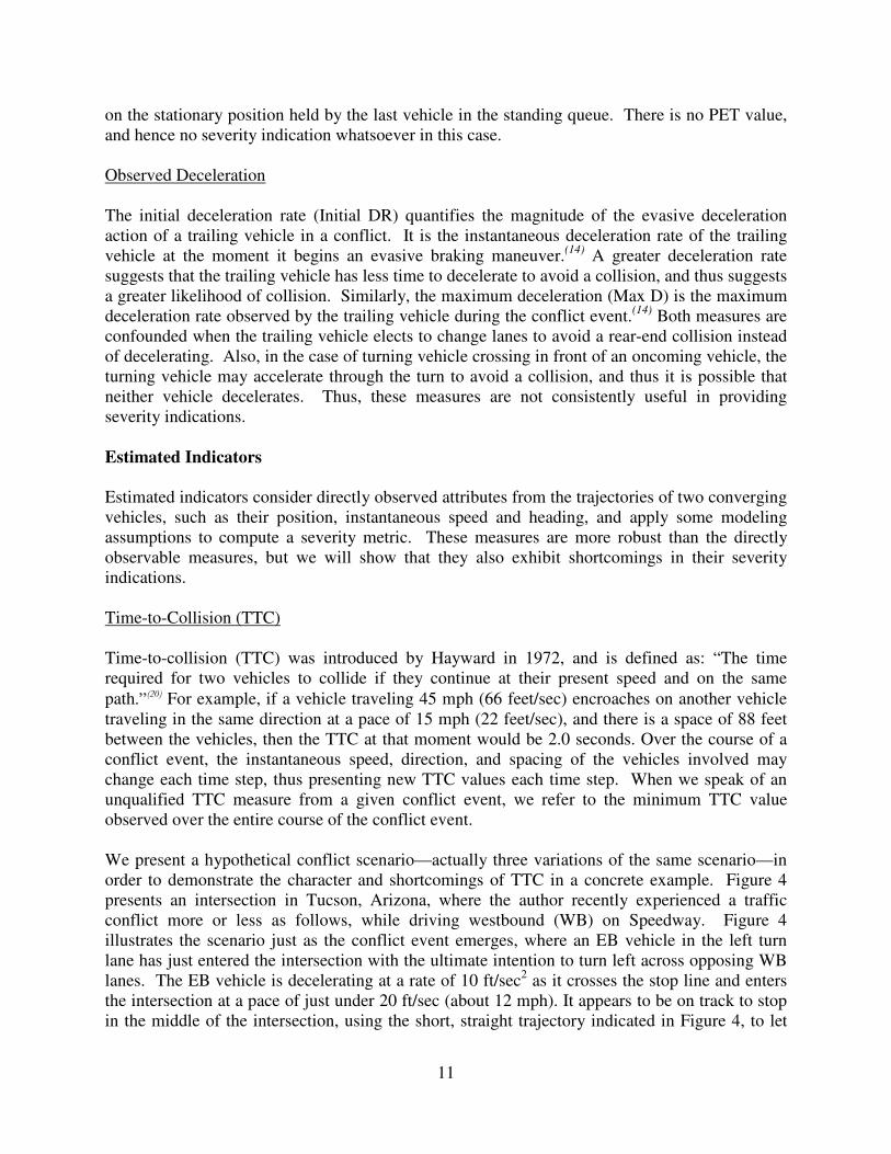
Estimated indicators consider directly observed attributes from the trajectories of two converging vehicles, such as their position, instantaneous speed and heading, and apply some modeling assumptions to compute a severity metric. These measures are more robust than the directly observable measures, but we will show that they also exhibit shortcomings in their severity indications. Time-to-Collision (TTC) Time-to-collision (TTC) was introduced by Hayward in 1972, and is defined as: “The time required for two vehicles to collide if they continue at their present speed and on the same path.”(20) For example, if a vehicle traveling 45 mph (66 feet/sec) encroaches on another vehicle traveling in the same direction at a pace of 15 mph (22 feet/sec), and there is a space of 88 feet between the vehicles, then the TTC at that moment would be 2.0 seconds. Over the course of a conflict event, the instantaneous speed, direction, and spacing of the vehicles involved may change each time step, thus presenting new TTC values each time step. When we speak of an unqualified TTC measure from a given conflict event, we refer to the minimum TTC value observed over the entire course of the conflict event. We present a hypothetical conflict scenario—actually three variations of the same scenario—in order to demonstrate the character and shortcomings of TTC in a concrete example. Figure 4 presents an intersection in Tucson, Arizona, where the author recently experienced a traffic conflict more or less as follows, while driving westbound (WB) on Speedway. Figure 4 illustrates the scenario just as the conflict event emerges, where an EB vehicle in the left turn lane has just entered the intersection with the ultimate intention to turn left across opposing WB lanes. The EB vehicle is decelerating at a rate of 10 ft/sec2 as it crosses the stop line and enters the intersection at a pace of just under 20 ft/sec (about 12 mph). It appears to be on track to stop in the middle of the intersection, using the short, straight trajectory indicated in Figure 4, to let

12

oncoming WB vehicles pass before completing its turn. However, the vehicle suddenly accelerates and initiates the left turn in front of the oncoming WB vehicle, using the path indicated by the sweeping arc across the intersection. Its path cuts across the path of the oncoming WB lane at approximately a 45-degree angle. The conflict area is the white rhombus-shaped zone with cross-hatched marking in the middle of the intersection. This hypothetical conflict resolves itself without incident, due to the turning vehicle accelerating at a maximum acceleration pace through the remainder of the movement. We assumed a linearly decreasing acceleration model.(21) The projected collision vanishes after 1.3 seconds (reaching a minimum TTC of 1.5 seconds), when the vehicle has accelerated to nearly 17 mph. The turning vehicle clears the conflict area just a moment before with the WB vehicle arrives, without the WB vehicle having to decelerate.

Figure 4. Left-turn crossing conflict scenarios. Background image from Google Earth.

There are three variations of this scenario. Each entails only a singular vehicle in the WB through lane that reaches a minimum time-to-collision of 1.5 seconds, with specific variations as follows:

13

•••• Scenario A – The WB vehicle, marked A, is traveling at 30 mph when a collision course emerges with a TTC of 2.8 seconds, at a distance of 123 feet from the conflict area. The conflict reaches its minimum TTC of 1.5 seconds at a distance of 66 feet from the conflict zone when the left turning vehicle has accelerated to a pace at which it would clear the conflict zone before the WB vehicle arrives. The WB vehicle and EB vehicle are both typical mid-size sedans weighing 3,487 pounds and measuring 15.8 feet in length with 6.0 feet wide.

•••• Scenario B – The WB vehicle, marked B, is traveling at 45 mph when a collision course

emerges with a TTC of 2.8 seconds, at a distance of 185 feet from the conflict area. The conflict reaches its minimum TTC of 1.5 seconds at a distance of 99 feet from the conflict zone when the left turning vehicle has accelerated to a pace at which it would clear the conflict zone before the WB vehicle arrives. The vehicles are equally sized, with dimensions as in Scenario A.

•••• Scenario C – The WB vehicle, marked C, is traveling at 45 mph when a collision course

emerges with a TTC of 2.8 seconds, at a distance of 185 feet from the conflict area. The conflict reaches its minimum TTC of 1.5 seconds at a distance of 99 feet from the conflict zone when the left turning vehicle has accelerated to a pace at which it would clear the conflict zone before the WB vehicle arrives. The WB vehicle is a typical large SUV, weighing 5,411 pounds, while the EB vehicle is a typical compact car weighing 2,979.

We now consider the relative collision propensity and potential crash severity of these scenarios, which all have identical TTC values of 1.5 seconds (i.e., identical traditional measures of severity). Consider the calculation of ∆v, adopting the TTC assumption that severity can be gauged by assuming vehicles maintain their speed and path until impact. The velocity of the turning vehicle at the minimum TTC moment is approximately 17 mph, in the north-easterly direction. Purely in the interest of a more tractable example, we will simplify matters into a one-dimensional realm (along an East-West axis), and thus consider only the EB component of the velocity, which would have a speed of approximately 8.5 mph.

•••• In Scenario A, the WB vehicle was traveling at a pace of 30 mph. The ∆v for this scenario is 19.25 mph, which corresponds to a probability of injury of 0.038 and a probability of fatality of 0.003.

•••• In Scenario B, the WB vehicle was traveling at a pace of 45 mph. The ∆v for this

scenario is 26.75 mph, which corresponds to a probability of injury of 0.089 and a probability of fatality of 0.013.

•••• In Scenario C, the WB vehicle was traveling at a pace of 45 mph, and in this case the WB

vehicle mass is approximately 1.8 times the size of the EB vehicle. The ∆v for the larger WB vehicle is 19 mph, which corresponds to a probability of injury of 0.036 and a probability of fatality of 0.003. The ∆v for the smaller WB vehicle is 34.5 mph, which corresponds to a probability of injury of 0.173 and a probability of fatality of 0.042.

14

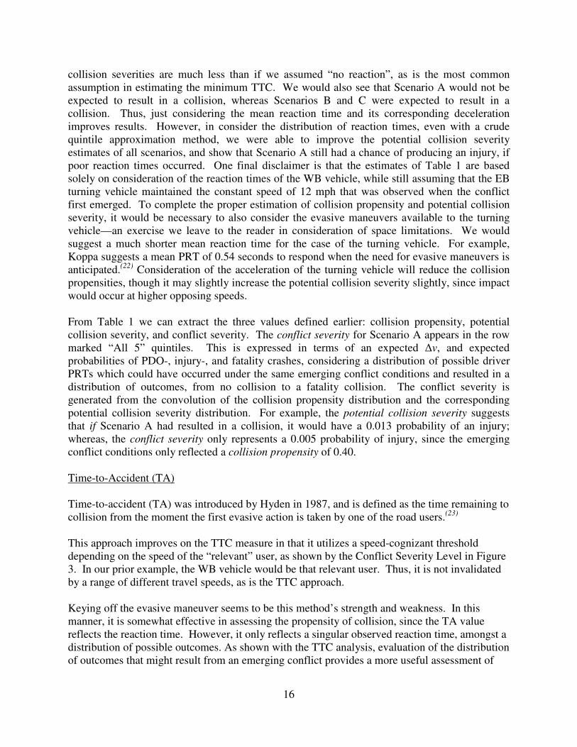
Despite the indication by the TTC values that these three conflict scenarios have identical severity, these simplistic ∆v calculations suggest that Scenario B is 4.3 times more likely to result in a fatality than Scenario A, and Scenario C is 14 times more likely to result in a fatality than Scenario A. While these calculations very simplified, it remains clear that these scenarios have dramatically different potential collision severities. We now turn our attention to an estimation of collision propensities. To calculate a credible expectation of collision, we suggest returning to the point where the traffic conflict emerged, which is to say to first moment when a collision course seemed possible. This occurred with a TTC value of 2.8 seconds. In contrast, typical applications of TTC only consider conflicts below a specified TTC threshold, which most commonly is 1.5 seconds. In that context, it would only be necessary to project vehicle trajectories 1.5 seconds into the future, looking for possible collisions. Our example scenarios have been constructed explicitly to illustrate the arbitrariness of the TTC threshold approach. With just the slightest adjustment to speed or spacing, each of these example scenarios would exceed the threshold, and thus be entirely discarded, despite having only the slightest reduction of their collision propensity and potential collision severity. Higher speeds, such as freeway facilities, warrant longer thresholds. However, setting TTC thresholds to higher values results in the identification of many “safe” conflicts, which do not indicate hazards (another shortcoming of the TTC approach). As an alternative to a fixed, arbitrary threshold, we suggest a projection horizon (i.e., the duration of the look-ahead for a potential collision) that is based on the time to travel, at current speed, over the distance necessary to identify a hazard and decelerate to a complete stop. In our example, vehicles were traveling as high as 45 mph, which would correspond to a projection horizon of 4.17 seconds. This assumes an average perception-reaction time (PRT) of 1.3 seconds, which is based on studies of recognizing and responding to stimulus to decelerate from a forward-looking perspective.(22) A more robust projection horizon would incorporate uncertainty, such as recognizing that 95th percentile reaction time, which would be about 2.45 seconds, extending the projection horizon to 5.32 seconds. It is also evident that reaction times are dependent on the situation, and are often longer for recognizing a threat coming from the side. Similarly, a longer projection horizon could be warranted by large trucks, which would not be capable of stopping as quickly as passenger cars. In this example, the conflict with a TTC of 2.8 seconds was identified as it emerged. From this point in time, we consider the log-normally distributed perception reaction time behavior, which from human factors studies assume in this case to have a mean a 1.3 seconds, and a standard deviation of 0.61 seconds.(22) Table 1 considers quantizing the probability distribution of the WB vehicle’s perception reaction time into quintiles (i.e., 5 equal portions of the distribution). The perception reaction time could certainly be quantized to a finer resolution than quintiles for better accuracy, though that increases the computational burden, so we have chosen quintiles as a practical matter to keep this example simple to manually-calculate, both for the author and readers interested in replicating the example calculations. Each quintile can be evaluated by considering its midpoint percentile. For example, the first quintile considers the shortest perception reaction times in the range of 0 percentile to 20th percentile. The midpoint of this range is the 10th percentile, which corresponds to reaction time of 0.67 seconds. We calculate the impact velocity (if any) assuming that the WB

15

vehicle begins decelerating 0.67 seconds after the conflict emerges, at an emergency rate of 14.8 ft/sec2 (as suggested by AASHTO). However, for the first quintile, Scenario A does not result in contact, since the WB vehicle could decelerate to a stop before the conflict zone if it reacted that quickly. Table 1. Distribution of reaction times and resulting outcomes.

Inspecting Table 1, it is evident through this quintile approximation scheme that Scenario A will not result in a collision if reaction times of the WB driver are within the first 3 quintiles. The fourth quintile, with a midpoint reaction time of 1.5 seconds, did result in a collision, though the WB vehicle was able to decelerate to a low speed. Had we quantized the reaction time distribution with greater resolution, we could have deduced that for a reaction time of 1.32 or more, the WB vehicle in Scenario A would not be able to stop in time. That would be a 59th percentile reaction time, which suggests a collision propensity of 0.41; however, with the quintile approximation, we were able to estimate a propensity of 0.40, which was fairly close. Note that the higher speed vehicles in Scenarios B and C presented an approximate collision propensity of 0.60. A higher resolution quantized distribution would reveal a more precise collision propensity of 0.63. From this analysis, it is plainly evident that the collision propensities of Scenarios B and C were significantly higher than the propensity of Scenario A, despite having the same TTC values.

There are a couple other important observations from Table 1. First, by considering the mean reaction times, and explicitly accounting for deceleration, we would see that the potential

Scenario Quintile Percentile PRT (sec) P{collision} Delta V P{PDO} P{injury} P{fatality} E[loss]

A 1 10 0.67 0.00 0.00 0.000 0.000 0.000 -$

A 2 30 0.94 0.00 0.00 0.000 0.000 0.000 -$

A 3 50 1.19 0.00 0.00 0.000 0.000 0.000 -$

A 4 70 1.50 0.20 9.60 0.994 0.006 0.000 3,102$

A 5 90 2.10 0.20 15.20 0.980 0.020 0.001 6,386$

B 1 10 0.67 0.00 0.00 0.000 0.000 0.000 -$

B 2 30 0.94 0.00 0.00 0.000 0.000 0.000 -$

B 3 50 1.19 0.20 16.10 0.977 0.023 0.001 7,468$

B 4 70 1.50 0.20 18.80 0.965 0.035 0.003 12,218$

B 5 90 2.10 0.20 22.90 0.941 0.059 0.006 25,638$

C 1 10 0.67 0.00 0.00 0.000 0.000 0.000 -$

C 2 30 0.94 0.00 0.00 0.000 0.000 0.000 -$

C 3 50 1.19 0.20 20.80 0.954 0.046 0.004 17,634$

C 4 70 1.50 0.20 24.20 0.932 0.068 0.008 32,058$

C 5 90 2.10 0.20 29.50 0.885 0.115 0.020 74,047$

A All 5 All 5 All 5 0.40 4.96 0.395 0.005 0.000 1,897$

B All 5 All 5 All 5 0.60 11.56 0.576 0.024 0.002 9,065$

C All 5 All 5 All 5 0.60 14.90 0.554 0.046 0.007 24,748$

A No reaction ≥ 2.80 1.00 19.30 0.962 0.038 0.003 13,399$

B No reaction ≥ 2.80 1.00 26.80 0.911 0.089 0.013 49,067$

C No reaction ≥ 2.80 1.00 34.50 0.827 0.173 0.042 147,114$

A Mean 1.31 0.00 0.00 0.000 0.000 0.000 -$

B Mean 1.31 1.00 17.20 0.972 0.028 0.002 9,104$

C Mean 1.31 1.00 22.20 0.946 0.054 0.006 22,669$

16

collision severities are much less than if we assumed “no reaction”, as is the most common assumption in estimating the minimum TTC. We would also see that Scenario A would not be expected to result in a collision, whereas Scenarios B and C were expected to result in a collision. Thus, just considering the mean reaction time and its corresponding deceleration improves results. However, in consider the distribution of reaction times, even with a crude quintile approximation method, we were able to improve the potential collision severity estimates of all scenarios, and show that Scenario A still had a chance of producing an injury, if poor reaction times occurred. One final disclaimer is that the estimates of Table 1 are based solely on consideration of the reaction times of the WB vehicle, while still assuming that the EB turning vehicle maintained the constant speed of 12 mph that was observed when the conflict first emerged. To complete the proper estimation of collision propensity and potential collision severity, it would be necessary to also consider the evasive maneuvers available to the turning vehicle—an exercise we leave to the reader in consideration of space limitations. We would suggest a much shorter mean reaction time for the case of the turning vehicle. For example, Koppa suggests a mean PRT of 0.54 seconds to respond when the need for evasive maneuvers is anticipated.(22) Consideration of the acceleration of the turning vehicle will reduce the collision propensities, though it may slightly increase the potential collision severity slightly, since impact would occur at higher opposing speeds. From Table 1 we can extract the three values defined earlier: collision propensity, potential collision severity, and conflict severity. The conflict severity for Scenario A appears in the row marked “All 5” quintiles. This is expressed in terms of an expected ∆v, and expected probabilities of PDO-, injury-, and fatality crashes, considering a distribution of possible driver PRTs which could have occurred under the same emerging conflict conditions and resulted in a distribution of outcomes, from no collision to a fatality collision. The conflict severity is generated from the convolution of the collision propensity distribution and the corresponding potential collision severity distribution. For example, the potential collision severity suggests that if Scenario A had resulted in a collision, it would have a 0.013 probability of an injury; whereas, the conflict severity only represents a 0.005 probability of injury, since the emerging conflict conditions only reflected a collision propensity of 0.40. Time-to-Accident (TA) Time-to-accident (TA) was introduced by Hyden in 1987, and is defined as the time remaining to collision from the moment the first evasive action is taken by one of the road users.(23) This approach improves on the TTC measure in that it utilizes a speed-cognizant threshold depending on the speed of the “relevant” user, as shown by the Conflict Severity Level in Figure 3. In our prior example, the WB vehicle would be that relevant user. Thus, it is not invalidated by a range of different travel speeds, as is the TTC approach. Keying off the evasive maneuver seems to be this method’s strength and weakness. In this manner, it is somewhat effective in assessing the propensity of collision, since the TA value reflects the reaction time. However, it only reflects a singular observed reaction time, amongst a distribution of possible outcomes. As shown with the TTC analysis, evaluation of the distribution of outcomes that might result from an emerging conflict provides a more useful assessment of

17

the collision propensity and collision severity than were obtained by just considering the mean reaction time. A remaining issue is how exactly to discern when an evasive action occurs. This issue is analogous to the course projection issue with TTC, where human observers can naturally perceive an evasive maneuver from a non-evasive maneuver; however, codifying this technique for automated algorithms presents a challenge. In our previous example, it is not clear where the evasive maneuver begins. The turning vehicle was accelerating throughout the conflict. Thus, there was a “change in speed”, which from one perspective may be an evasive reaction, but not an easily distinguished change in strategy or intention since the acceleration was steady. After 1.3 seconds of acceleration, the turning vehicle reached a pace where the collision course vanished. Since the mean reaction time of the WB vehicle was 1.3 seconds, and the collision course was no longer present at the end of that response time, it is possible that the WB vehicle would not have reacted at all, exhibiting no evasive maneuver. If we assume that the acceleration of the turning vehicle constitutes the evasive action, then the TA value would be 2.8 seconds. For Scenario A, with the WB vehicle approaching at 30 mph (48.3 km/hr), we can see from Figure 3 that a TA of 2.8 seconds leaves too much time remaining (i.e., does not exceed the Conflict Severity Level), and thus Scenario A would not be counted as a conflict. The other scenarios with a 45 mph (72.4 km/hr) approach speed would just exceed the minimum severity level. It seems inappropriate to abandon Scenario A, which exhibited a significant collision propensity (although those calculations were not completed to incorporate the behavior of the turning vehicle). However, such is the nature of any binary “threshold” based scheme, that a hazard is either a conflict or it is not (i.e., black or white). Note that our suggested projection horizon casts a much wider net, with a 3.2-second horizon for Scenario A, as opposed to the 2.0 second threshold imposed by the Swedish method. By explicitly calculating a collision propensity (i.e., spanning whole grayscale spectrum), the approach we demonstrate is able to incorporate less “serious” conflicts into the overall safety assessment. The ambiguity of the definition of “evasive maneuver” is perhaps what make some researchers call the TTC approach more objective (than TA).(3) We will assume, for the sake of argument, that the WB vehicle did decelerate, and that this happened 1.3 seconds after the conflict emerged. At that moment, the remaining TA value was 1.5 seconds. In this case, the TA/CS severity indicator accurately differentiates Scenario A as less “severe” than Scenarios B and C. However, the TA/CS value would be the same value for both Scenario B and Scenario C. In the last section, we showed the Scenario C was 3 times more likely to result in a fatality than Scenario B. Thus, in overlooking the impact of relative vehicle mass on severity, the Swedish Traffic Conflict Technique exhibits a significant shortcoming in discerning severity levels. Similarly, were it the case that the heavier vehicle were unable to decelerate as fast as the lighter vehicle, perhaps the collision propensities of scenarios B and C would be different, with Scenario C being more likely to result in an accident. It does not seem that TA accounts for the different characteristics of different vehicles. It is also evident that the TA approach would not distinguish a crossing vehicle that was accelerating at a partially opposing angle (as in our example) from a crossing vehicle at a perpendicular angle that was not accelerating. Certainly, the combination of both vehicles taking evasive action would tend to reduce the collision propensity more so than

18

just one vehicle reacting. TA and TA/CS indicators have no mechanism to account for this difference in collision propensities. We have shown an example where the estimated indicators of severity, TTC and TA, both rated two traffic conflicts (Scenario B and Scenario C) with identical severity values, yet these scenarios presented drastically different severities, with Scenario C being more than 3 times more likely to result in a fatality. NOT ALL CRASHES ARE EQUAL … RIGHT?

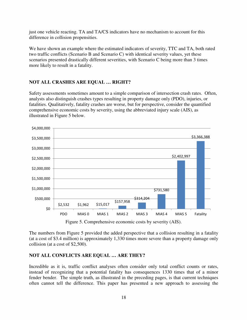
Safety assessments sometimes amount to a simple comparison of intersection crash rates. Often, analysts also distinguish crashes types resulting in property damage only (PDO), injuries, or fatalities. Qualitatively, fatality crashes are worse, but for perspective, consider the quantified comprehensive economic costs by severity, using the abbreviated injury scale (AIS), as illustrated in Figure 5 below.

Figure 5. Comprehensive economic costs by severity (AIS).

The numbers from Figure 5 provided the added perspective that a collision resulting in a fatality (at a cost of $3.4 million) is approximately 1,330 times more severe than a property damage only collision (at a cost of $2,500). NOT ALL CONFLICTS ARE EQUAL … ARE THEY?

Incredible as it is, traffic conflict analyses often consider only total conflict counts or rates, instead of recognizing that a potential fatality has consequences 1330 times that of a minor fender bender. The simple truth, as illustrated in the preceding pages, is that current techniques often cannot tell the difference. This paper has presented a new approach to assessing the

$2,532 $1,962 $15,017$157,958

$314,204

$731,580

$2,402,997

$3,366,388

$0

$500,000

$1,000,000

$1,500,000

$2,000,000

$2,500,000

$3,000,000

$3,500,000

$4,000,000

PDO MIAS 0 MIAS 1 MIAS 2 MIAS 3 MIAS 4 MIAS 5 Fatality

19

severity of traffic conflicts through the estimation of Delta-V. This approach also directly estimates of collision propensity, as a distinctly different characteristic of a traffic conflict, by incorporating estimates of the distribution of driver reaction times at the moment a traffic conflict emerges. Whereas prevailing techniques using TTC or TA values utilize a threshold to classify a vehicle encounter as either a conflict or not, the approach demonstrated in this paper gauges each encounter with a collision propensity spanning the whole range from zero to one. Furthermore, this approach demonstrates utilizing Delta-V to gauges the probability of injuries of different severities. By combining a collection of observed conflict encounters, their distribution of collision propensities, their distribution of potential collision severities, and the associated comprehensive economic costs of each potential outcome, it would certainly seem plausible to better assess the relative safety of two traffic facilities than possible by employing current schemes that often fail to distinguish all of these important characteristics. The rightmost column of Table 1 provides the expected compressive cost (i.e., loss) for our example. CONCLUSIONS

This paper introduced the concept of Delta-V (∆v) as a measure for the severity of traffic conflicts, and showed how it overcomes significant shortcomings present in several of the most commonly used surrogate safety indicators, including time-to-collision and time-to-accident measures. We reviewed various conflict severity terms used in the literature, and proposed alternative terms and interpretations to bring clarity to the topic. An example was presented to demonstrate how to directly estimate collision propensity, and use ∆v to estimate the probability of PDO, injury, or fatality outcomes. This technique also introduces a full spectrum of “shades of gray”, valuing each conflict differently, instead of the traditional binary (black/white) classification scheme of using a threshold to judge an encounter as an “official” conflict or not. Finally, we have suggested combining comprehensive economic costs with explicit estimates of collisions of different severities, to obtain a more universal comparison of the full profile of traffic conflicts of different types, observed at different traffic facilities that are competing for a common pool of safety remediation funds. We feel that these new directions in traffic conflict analysis may yield substantially improved safety assessment results. REFERENCES

1. Gettman, D., Pu, L., Sayed, T., and Shelby, S., Surrogate Safety Assessment Model and

Validation: Final Report. Report No. FHWA-HRT-08-051. FHWA, 2008. 2. Hyden, C., The Swedish Traffic Conflicts Technique. Lund University,

http://www.lth.se/fileadmin/tft/dok/Brochure_ConflictTecnique.pdf, accessed 2010. 3. Archer, J., Indicators for traffic safety assessment and prediction and their applicaiton in

micro-simulation modelling: A study of urban and suburban intersections, in Department

of Infrastructure. Royal Institute of Technology: Stockholm, Sweden, 2005. 4. McHenry, R.R. The CRASH Program - A Simplified Collision Reconstruction Program.

in Motor Vehicle Collision Investigation Symposium. 1975: Calspan, 5. Sharma, D., Stern, S., Brophy, J., and Choi, E.-H. An Overview of NHTSA’s Crash

Reconstruction Software WinSMASH. in 20th International Technical Conference on the

Enhanced Safety of Vehicles. 2007, 6. Campbell, K.L., Energy Basis of Collision Severity. SAE Technical Papers, 1974.

20

7. Nordoff, L.S., Motor vehicle collision injuries: biomechanics, diagnosis, and

management. Jones and Bartless Publishers, Inc., 2005. 8. McHenry, R. and McHenry, B., Effect of Restitution in the Application of Crush

Coefficients. SAE Technical Papers No 970960, 1997. 9. Carlson, W.L., Crash Injury Prediction Model. Accident Analysis and Prevention, 11,

137-153, 1979. 10. Joksch, H.C., Velocity Change and Fatality Risk in a Crash - A Rule of Thumb. Accident

Analysis and Prevention, Vol. 25, No. 1, pp. 103-104, 1993. 11. Managing Speed: review of current practice for setting and enforcing speed limits.

Transportation Research Board, National Research Council, National Academy Press, 1998.

12. Joksch, H., Massie, D., and Pichler, R., Vehicle Aggressivity: Fleet Characterization

Using Traffic Collision Data. Report No. DOT-VNTSC-NHTSA-98-1. USDOT, 1998. 13. Evans, L., Drive Injury and Fatality Risk in Two-Car Crashes Versus Mass Ratio

Inferred Using Newtonian Mechanics. Accident Analysis and Prevention, Vol. 26, No. 5, pp. 609-616, 1994.

14. Gettman, D. and Head, L., Surrogate Safety Measures from Traffic Simulation Models. Transportation Research Record 1840, pp. 104-115, 2003.

15. Saunier, N., Sayed, T., and Lim, C. Probability Collision Prediction for Vision-Based

Automated Road Safety Analysis. in The 10th International IEEE Conference on

Intelligent Transportation Systems. 2007: IEEE, pp. 872-878. 16. Svensson, Å. A method for analysing the traffic process in a safety perspective. Bulletin

166, Lund Institute of Technology, Lund University, http://www.lth.se/fileadmin/tft/dok/KFBkonf/6AseSvensson.pdf, accessed 2010.

17. Svensson, A. and Hyden, C., Estimating the severity of safety related behaviour. Accident Analysis and Prevention, Vol. 38, pp. 379-385, 2006.

18. Sayed, T.A., A Simulation Model of Road User Behaviour and Traffic Conflicts at

Unsignalized Intersections, in Department of Civil Engineering. University of British Columbia: Vancouver, Canada, 1992.

19. Chin, H.-C. and Quek, S.-T., Measurement of Traffic Conflicts. Safety Science, Vol. 26, No. 3, pp. 169-185, 1997.

20. Hayward, J.C., Near-miss determination through use of a scale of danger. Highway Research Board, Research Record 384, pp. 24-34, 1972.

21. Long, G. Acceleration Characteristics of Starting Vehicles. in TRB 79th Annual Meeting. 2000,

22. Koppa, R.J., Human Factors, in Revised Monograph on Traffic Flow Theory. FHWA, 2000.

23. Hyden, C., The development of a method for traffic safety evaluation: the Swedish traffic

conflict technique, in Department of Traffic Planning and Engineering. Lund University: Lund, Sweden, 1987.