Deliverable D2.2 Second report on mathematical models · Second report on mathematical models Lead...
95
Grant Agreement No. 268478 Deliverable D2.2 Second report on mathematical models Lead partner for this deliverable: UVIGO Version: 2.0 Dissemination level: Public January 30, 2013
Transcript of Deliverable D2.2 Second report on mathematical models · Second report on mathematical models Lead...

Grant Agreement No. 268478
Deliverable D2.2
Second report on mathematical models
Lead partner for this deliverable: UVIGOVersion: 2.0
Dissemination level: Public
January 30, 2013
Contents
Introduction 4
1 Forensics vs Steganalysis 51.1 FA and ADST . . . . . . . . . . . . . . . . . . . . . . . . . . . . . . . . . . . . . . . . 51.2 ADFA and ST . . . . . . . . . . . . . . . . . . . . . . . . . . . . . . . . . . . . . . . . 61.3 Similarities . . . . . . . . . . . . . . . . . . . . . . . . . . . . . . . . . . . . . . . . . 71.4 Differences . . . . . . . . . . . . . . . . . . . . . . . . . . . . . . . . . . . . . . . . . . 81.5 Lessons to be learned . . . . . . . . . . . . . . . . . . . . . . . . . . . . . . . . . . . . 81.6 Links to previous works in the literature . . . . . . . . . . . . . . . . . . . . . . . . . 8
2 General theory 102.1 Source identification game with training sequences . . . . . . . . . . . . . . . . . . . 102.2 Taking advantage of source correlation in forensic analysis . . . . . . . . . . . . . . . 19
3 Operator chain modeling 313.1 JPEG Quantization and full-frame filtering . . . . . . . . . . . . . . . . . . . . . . . 313.2 Interpolation estimation . . . . . . . . . . . . . . . . . . . . . . . . . . . . . . . . . . 413.3 Transform coder identification based on quantization footprints and lattice theory . 513.4 Modeling reacquisition . . . . . . . . . . . . . . . . . . . . . . . . . . . . . . . . . . . 673.5 Demosaicking localization . . . . . . . . . . . . . . . . . . . . . . . . . . . . . . . . . 73
4 Synergies with WP3 and WP4 804.1 JPEG Quantization and full-frame filtering . . . . . . . . . . . . . . . . . . . . . . . 804.2 Transform coder identification based on quantization footprints and lattice theory . 834.3 Modeling reacquisition chains . . . . . . . . . . . . . . . . . . . . . . . . . . . . . . . 844.4 Demosaicking localization . . . . . . . . . . . . . . . . . . . . . . . . . . . . . . . . . 854.5 Double JPEG Compression Models . . . . . . . . . . . . . . . . . . . . . . . . . . . . 86
Appendix A Proof of Lemma 1 88
1

Acronyms and Abbreviations
AC Alternating CurrentAD AdversaryADFA Anti-Forensics PlayerADST SteganalyzerA/D Analog-to-DigitalAF Anti-ForensicsAR AutoregressiveAVC Advanced Video CodingCFA Color Filter ArrayD/A Digital-to-AnalaogDCT Discrete Cosine TransformDMS Discrete Memoryless SourceEM Expectation-MaximizationFA Forensics AnalystFRI Finite Rate of InnovationGCD Greatest Common DivisorGGD Generalized Gaussian DistributionGMM Gaussian Mixture ModelHEVC High Efficiency Video CodingHP High PassIDCT Inverse Discrete Cosine Transformi.i.d. Independent and Identically DistributedJPEG Joint Photographic Experts GroupKL Kullback-LeiblerLLL Lenstra-Lenstra-LovaszLP Low PassML Maximum LikelihoodMLE Maximum Likelihood EstimateMMF MultiMedia ForensicsMOMS Maximal-Order-Minimal-SupportMPEG Moving Picture Experts Grouppdf Probability Density Function
2

CONTENTS 3
pmf Probability Mass FunctionQF Quality FactorSI Source IdentificationST SteganographerTI Transform IdentificationTIFF Tagged Image File FormatUC Use CaseUCID Uncompressed Colour Image DatabaseWP Work Package

Introduction
This deliverable summarizes the work performed in months 13 to 21 in the scope of WP2. In thisperiod the originally planned schedule was followed, as it is reflected in the obtained results exposedin this report. Nevertheless, special attention has been also paid to the comments made by theproject reviewers. Specifically, two short chapters have been included for dealing with the similaritiesand differences between steganography and multimedia forensics (Chapter 1), and explaining threeexamples of the synergies between WP2, and WP3 and WP4 (Chapter 4). Besides these two shortchapters, the main results obtained in this period of 9 months are split in a chapter dealing withtheoretical general topics (Chapter 2), and other chapter studying the modeling of operator chain(Chapter 3).Within Chapter 2, results on identification source identification game with training sequences havebeen included. On the other hand Chapter 3 includes results on
• JPEG quantization followed by full-frame filtering
• Interpolation estimation
• Transform coder identification based on noiseless lattice estimation
• Reacquisition modeling
• Demosaicking localization
4

Chapter 1
Similarities and differencesbetween forensics and steganalysis
In the field of multimedia security one can distinguish different problems; probably watermarking,steganography, and lately forensics, are those that have received more attention. Hopefully, lookingat the evolution of the other problems of multimedia security will allow us to learn some lessonsabout good directions to be followed by multimedia forensics. Due to the shared statistical undis-tinguishability constraint, it seems that forensics is more closely related to steganalysis. Therefore,the target of this chapter is to study the main parallelisms, and corresponding similarities and dif-ferences between multimedia forensics and steganography; specifically, we will focus on the similarrole of forensics analyst and steganalyzer, and also on the similar target of counter-forensics playerand steganographer. Based on this discussion, we will summarize what are, in our opinion, the mainlessons to be learned. Finally, links to previous works in the literature will be pointed out.For the sake of notational simplicity, we will use MMF for denoting MultiMedia Forensics, AF forAnti-Forensics, FA for Forensics Analyst, ADFA for the anti-forensics player, ST for the steganogra-pher, and ADST for the steganalyzer.
1.1 FA and ADST
From the point of view of the FA we can consider MMF as an estimation problem (if we wantto estimate the processing parameters), or a binary hypothesis problem (if we want to decide if agiven content was modified or not, or in an alternative way, if it comes from source A or sourceB). ST counterparts to these two scenarios could be also considered, being the binary hypothesisversion the classical steganographic problem, and the estimation version the so-called “quantitativesteganalysis”.Therefore, the ADST’s formal description of the steganalysis problem is nothing but a particularexample of the FA’s MMF formal description; this is the case for both the estimation and binaryversions of the two problems. Some considerations must be taken into account :
• Kind of processing to be considered: We can consider a set of possible processing/modificationsas broad as we want, although in general some constraints are imposed in that set in orderto have a problem which is feasibly resolved. For example, we can focus our attention onthe case of JPEG quantization+spatial filtering, cut+paste+footprint removal, informationembedding+footprint removal (=steganography; in this case, the FA is indeed an ADST).
5

CHAPTER 1. FORENSICS VS STEGANALYSIS 6
Even smaller sets could be considered, e.g. MPSteg detection; as far as we reduce the set (orclass) of possible processing, we have a more targeted scheme (following steganalysis naming).Therefore, from that point of view, what distinguishes steganography as a particularcase of MMF is the analyzed set of feasible operators.
• If the null hypothesis does not only include the “no processing” case, but also some “lightprocessings” (meaning that the semantics of the content are not modified) are included, thenan additional multimedia security problem, namely authentication, could be also included inthis framework.1
• Summarizing, according to this approach the ADST is nothing but a FA using a particulardefinition of the alternative hypothesis H1, where the analyzed set of feasible operators onlycontains “stego-processing.”
Note that in the case of universal steganalyzers, the alternative hypothesis H1 is not well defined,since the embedding algorithm is not known. Therefore, one-class classifiers (or composite hypothesistesting) must be resorted. A similar conclusion can be derived for MMF.
1.2 ADFA and ST
Once the similarity between FA and ADST has been established, one wonders if this can be extendedto the similarity between ADFA and ST. Nevertheless, in this case there is an obvious differencebetween the target of these two players: while in AF the goal depends on the kind of processingthe ADFA wants to hide (histogram stretching, compression, resizing, etc.), in steganography thegoal is transmitting secret information. Deep changes in the proposed approaches are implied.Despite this difference on the target function, both ADFA and ST share the same constraints:
• Statistical undetectability.
• Perceptual distortion. Typically, the perceptual distortion used in steganographic applicationsdepends on the original signal (i.e., reference-based distortion measures are used). Nevertheless,in MMF the definition of such kind of measure is more involved; for example, for cut and pasteattacks, one wonders how a reference-based distortion measure can be defined. However,since the original signal will be typically not accessible to the receiver, the use of reference-based distortion measures can be criticized even in the steganographic framework. If blind(no-reference) distortion measures were used (e.g., [3]), then we can define the perceptualdistortion for both problems in much the same way.
From an application point of view, in both cases one must face the constrain of the processedimages looking natural to a human observer.
• The fact of the steganography problem having more players (legitimate decoder and possiblythe active warden) is “just” reflected on the definition of the target function the ST tries tomaximize.
• The ST strategy is defined by the embedding function, while the ADFA strategy is the manipu-lation function. In both cases the feasible set of strategies is defined as that set that contains allthose functions that modify the original content while verifying the previous contraints. This
1The reader who is not accustomed to the basics on detection and/or estimation theory is referred to [1, 2].

CHAPTER 1. FORENSICS VS STEGANALYSIS 7
set is the same for both problems. The only change is the embedding/manipulation functionwhich is chosen in each case, since the target function is different in both cases.
Nevertheless, the impact of this difference is not trivial. Indeed, this yields the overall goal tobe different, as well as the kind of used techniques to differ:
– In stego an integrated approach is often used, in which the embedding function is chosento verify the statistical imperceptibility constraint.
– On the other hand, in MMF the attacker often adopts a post processing approach: first,it applies the intended modification; then, it tries to remove traces without “spoiling”the result of the modification. This two-steps strategy should be used as long as theprocessing and the counterforensics steps are not carried out in different time instants, orby different players. Other scenario where it makes sense is that where several processingsteps are applied, and the footprints of all of them are deleted in a single final step.
Nevertheless, probably there is not any fundamental reason for working in this case. For exam-ple, one could introduce the watermark in the content (without caring about the detectabilityconstraint, e.g., using regular watermark embedding techniques) and then apply some post-processing for removing the traces (reducing detectability). Alternatively, the MMF attackercould devise the content modification taking in mind the detectability constraint. In general,it seems that the two steps procedure (first doing the work and then solving the problems itentails) will behave worse than the one step approach.
Consequently, it seems that the only reason for applying two-steps attacks is the complexityreduction; being the application scenario requirements (including complexity ones) for ADFA
and ST completely different, is not surprising that different approaches to both problems havebeen developed.
Summarizing, one can state that ADFA and ST techniques are very different. This was notthe case with the MMF FA and ADST, which basically share the same techniques (classifiers,decision making, hypothesis testing, etc.).
1.3 Similarities
S1. The task of the ADST can be seen as a particular MMF task: detect the traces introduced bythe ST. Indeed, its task can be interpreted as completely equivalent to detecting the tracesleft by any other processing tool. This makes steganalysis a particular instance of MMF.
S2. Quantitative steganalysis is a particular case of MMF, assuming that the FA does not onlywant to detect processing traces but also to estimate some of the parameters characterizingthe processing.
S3. The constraints of the ST and the ADFA are also virtually identical, since both of them wantto modify a media (for different purposes) without leaving any kind (visible or statistical) oftrace. In this sense, steganography and anti-forensics are optimization problems that sharethe same feasible set but differ in their target functions.
S4. Cachin’s perfect steganography [4] is similar to statistics preserving AF.
S5. Steganalysis and MMF share the difficulty deriving from the lack of a good statistical modeldescribing natural images.

CHAPTER 1. FORENSICS VS STEGANALYSIS 8
1.4 Differences
D1. Despite similarity number 3, steganography and AF are quite different since their ultimate goalis very different: in AF the goal depends on the kind of processing the ADFA wants to hide(histogram stretching, compression, resizing, etc.); in steganography the goal is transmittingsecret information.
D2. In Steganography we have 3 players, while in MMF we usually have 2.
D3. MMF is a much wider field, encompassing issues extraneous to steganography and steganalysis:this is the case, for instance, of semantic-level MMF, like some works by Farid’s group (e.g.,[5]). In these cases MMF resembles more computer vision than stego.
D4. The batch steganography concept does not seem to apply to MMF.
D5. Similarities exist only with steganography by cover modification, while steganography by coverselection has nothing to share with MMF.
D6. From an application perspective stego and MMF are completely different, leading to ratherdifferent constraints (if not goals), e.g., amount of images to be analyzed, target error proba-bilities, etc.
1.5 Lessons to be learned
1. In the past years steganalysis has passed from classifiers based on few features, to a moderateamount of features until the very large number of features characterizing the most powerfulschemes developed recently. One wonders if MMF should follow the same path.
2. In early days, steganography was focused on statistical indistinguishability, i.e., the ST wasaiming at keeping some statistical quantities untouched. More recently, it seems that mini-mizing a properly defined distortion measure is a better choice. It is possible that AF will gothrough the same path.
3. Calibration has played a crucial role in steganalysis. Similar techniques can be borrowed forAF.
4. Steganalysis has switched from first order to higher order statistical analysis (and finally toclassifiers with a large number of features). Again, it is possible for MMF to follow the sameroute.
5. Steganographers typically use one-step strategies, while most of ADFA’s approaches are basedon two steps. Since the two steps approach is in general suboptimal, one wonders if the one-stepstrategies should be also adopted in counterforensics.
1.6 Links to previous works in the literature
The similarities and differences between steganography and counter-forensics are also studied in [6].In that work the authors point out that both steganography and counter-forensics try to hide thevery fact of a class change, and their success can be measured by the Kullback-Leibler divergence.Nevertheless, they also defend that steganography differs from counter-forensics in the amount and

CHAPTER 1. FORENSICS VS STEGANALYSIS 9
source of information to hide. These considerations are developed in our previous analysis, wherethey are stated in terms of the target function and the optimization search space constraints.Similarly, the connections between steganalysis and the forensics analyst, as well as the differencebetween one-step and two-steps attacks (typically used in steganography and counter-forensics, re-spectively) are also mentioned.

Chapter 2
General theory
2.1 Source identification game with training sequences
In the attempt to provide a mathematical background to multimedia forensics, we introduce thesource identification game with training data. The game models a scenario in which a forensicanalyst has to decide whether a test sequence has been drawn from a source X or not. In turn, theadversary takes a sequence generated by a different source and modifies it in such a way to induce aclassification error. The source X is known only through one or more training sequences. We derivethe asymptotic Nash equilibrium of the game under the assumption that the analyst relies only onfirst order statistics of the test sequence. A geometric interpretation of the result is given togetherwith a comparison with a similar version of the game with known sources. The comparison betweenthe two versions of the games gives interesting insights into the differences and similarities of thetwo games.1
2.1.1 Introduction
Understanding the fundamental limits of multimedia forensics in an adversarial environment is apressing need to avoid the proliferation of forensic and anti-forensic tools each focused on counteringa specific action of the adversary but prone to yet another class of attacks and counter-attacks. Themost natural solution to avoid entering this never-ending loop is to cast the forensic problem intoa game-theoretic framework and look for the optimum strategies the players of the game (usually aforensic analyst and an adversary) should adopt. Some early attempts in this direction can be foundin [9] and [10]. In [9], the authors introduce a game-theoretic framework to evaluate the effectivenessof a given attacking strategy and derive the optimal countermeasures. In [9] the attacker’s strategyis fixed and the game-theoretic framework is used only to determine the optimal parameters of theforensic analysis and the attack. A more general approach is adopted in [10], where the sourceidentification game with known statistics, namely the SIks game, is introduced. According to theframework defined in [10], given a discrete memoryless source (DMS) X with known statistics PX ,it is the goal of the Forensic Analyst (FA) to decide whether a test sequence xn has been drawnfrom X or not. In doing so, he has to ensure that the false positive probability, i.e. the probabilityof deciding that the test sequence has not been generated by X when it actually was, stays belowa predefined maximum value. The goal of the adversary (AD) is to take a sequence generated froma different and independent source Y ' PY and modify it so to let the FA think that the modified
1The reader who is not accustomed to the basics on game theory is referred to [7, 8].
10
CHAPTER 2. GENERAL THEORY 11
sequence has been generated by X. In doing so the AD must satisfy a distortion constraint, i.e.the distance between the original and the modified sequence must be lower than a threshold. Thepayoff of the AD is the false negative error probability, i.e. the probability that the FA classifies asequence drawn from Y and further modified by the AD as a sequence drawn from X. The oppositepayoff applies to the FA, thus qualifying the SIks as a zero-sum, competitive game [11]. Under thefurther assumption that the FA relies only on first order statistics (limited resources assumption)for his analysis and that the sources X and Y are memoryless, the asymptotic Nash equilibrium ofthe game can be found [10, 12], thus defining the optimum strategies for the FA and the AD whenthe length of the test sequence tends to infinity. A problem with the analysis carried out in [10] isthe assumption that the FA and the AD know the probability mass function (pmf) of the sourceX. This is not the case in many practical scenarios where sources are known only through one ormore training sequences. It is the goal of this chapter to reformulate the analysis carried out in [10]to address this new more realistic version of the game. As a main result, we derive the asymptoticNash equilibrium of the new game, hereafter referred to as the SItr game, under the same limitedresources assumptions used in [10]. In doing so we will discover that the optimal strategies for theFA and the AD deviate from those of the SIks game. In addition, at least in the case that thetraining sequences available to the FA and the AD coincide, we can show that passing from the SIksto the SItr version of the game is to the AD’s advantage.The description of the work is organized as follows. In section 2.1.2 we introduce the notation thatwill be used throughout the description. In section 2.1.3, we give a rigorous definition of the sourceidentification with training data game. In section 2.1.4, we derive the asymptotic Nash equilibriumof the game. In section 2.1.5, we compare the results obtained in this work with those referringto source identification with known sources. Section 2.1.6 concludes the description with someperspective for future research.
2.1.2 Notation
In the rest of this chapter we will use capital letters to indicate discrete memoryless sources (e.g. X).Sequences of length n drawn from a source will be indicated with the corresponding lowercase letters(e.g. xn). In the same way, we will indicate with xi, i = 1, n the i−th element of a sequence xn.The alphabet of an information source will be indicated by the corresponding calligraphic capitalletter (e.g. X ). Calligraphic letters will also be used to indicate classes of information sources (C).The pmf of a discrete memoryless source X will be denoted by PX . With a slight abuse of notation,the same symbol will be used to indicate the probability measure ruling the emission of sequencesfrom X, so we will use the expressions PX(a) and PX(xn) to indicate, respectively, the probabilityof symbol a ∈ X and the probability that the source X emits the sequence xn. Given an event A(be it a subset of X or Xn), we will use the notation PX(A) to indicate the probability of the eventA under the probability measure PX .Our analysis relies heavily on the concepts of type and type class defined as follows (see [13] and [14]for more details). Let xn be a sequence with elements belonging to an alphabet X . The type Pxn ofxn is the empirical pmf induced by the sequence xn, i.e. ∀a ∈ X , Pxn(a) = 1
n
∑ni=1 δ(xi, a). In the
following we indicate with Pn the set of types with denominator n, i.e. the set of types induced bysequences of length n. Given P ∈ Pn, we indicate with T (P ) the type class of P , i.e. the set of allthe sequences in Xn having type P .The Kullback-Leibler (KL) divergence between two distributions P andQ on the same finite alphabetX is defined as:
D(P ||Q) =∑a∈X
P (a) logP (a)
Q(a), (2.1)

CHAPTER 2. GENERAL THEORY 12
where, as usual, 0 log 0 = 0 and p log p/0 = ∞ if p > 0. Empirical distributions can be usedto calculate empirical information theoretic quantities, like, for instance, the empirical divergencebetween two sequences D(Pxn ||Pyn).As we said, the goal of this study is to cast the source identification problem into a game-theoreticframework, wherein identification is seen as a two-player, strategic, zero-sum game. In rigor-ous terms, a game is defined as a 4-tuple G(S1,S2, u1, u2), where S1 = {s1,1 . . . s1,n1
} and S2 ={s2,1 . . . s2,n2
} are the set of strategies (actions) the first and the second player can choose from, andul(s1,i, s2,j), l = 1, 2 is the payoff of the game for player l, when the first player chooses the strategys1,i and the second chooses s2,j . A pair of strategies s1,i and s2,j is called a profile. In a zero-sumcompetitive game, the two payoff functions are strictly related to each other since for any profile wehave u1(s1,i, s2,j)+u2(s1,i, s2,j) = 0. A zero-sum game, then reduces to a triplet G(S1,S2, u), wherewe have assumed u = u1 = −u2. Note that in strategic games the players choose their strategiesbefore starting the game so that they have no hints about the strategy actually chosen by the otherplayer. We say that a profile (s1,i∗ , s2,j∗) represents a Nash equilibrium if [15, 11]:
u1((s1,i∗ , s2,j∗)) ≥ u1((s1,i, s2,j∗)) ∀s1,i ∈ S1
u2((s1,i∗ , s2,j∗)) ≥ u2((s1,i∗ , s2,j)) ∀s2,j ∈ S2,(2.2)
where for a zero-sum game −u2 = u1 = u.
2.1.3 Source identification with training data
Let C be the class of discrete memoryless sources with alphabet X , and let X ' PX be a sourcein C. Given a test sequence xn, the goal of the Forensic Analyst (FA) is to decide whether xn wasdrawn from X or not2. As opposed to the source identification game with known sources [10], herewe assume that the FA does not know PX , and that he has to base his decision by relying on theknowledge of a training sequence tNFA drawn from X. On his side, the Adversary (AD) takes asequence yn emitted by another source Y ' PY still belonging to C and tries to modify it in such away that the FA thinks that the modified sequence was generated by X. In doing so the AD mustsatisfy a distortion constraint stating that the distance between the modified sequence, say zn, andyn must be lower than a predefined threshold. As the FA, the AD knows PX through a trainingsequence tKAD, that in general may be different than tNFA. We assume that tNFA, tKAD, xn and yn aregenerated independently. With regard to PY , we could also assume that it is known through twotraining sequences, one available to the FA and one to the AD, however we will see that - at leastto study the asymptotic behavior of the game - such an assumption is not necessary, and hence wetake the simplifying assumption that PY is known neither to the FA nor to the AD. As in [10], wedefine the game by casting the identification problem into a hypothesis decision framework. Letthen H0 be the hypothesis that the test sequence has been generated by X (i.e. the same sourcethat generated tNFA) and let Λ0 be the acceptance region for H0 (similarly we indicate with Λ1 = Λc0the rejection region for H0). We have the following:
Definition 1. The SItr,a(SFA,SAD, u) game is a zero-sum, strategic, game played by the FA andthe AD, defined by the following strategies and payoff.
• The set of strategies the FA can choose from is the set of acceptance regions for H0 for which themaximum false positive probability across all possible PX ∈ C is lower than a certain threshold:
SFA = {Λ0 : maxPX∈C
PX{(xn, tNFA) /∈ Λ0} ≤ Pfp}, (2.3)
2With a slight abuse of notation we use the symbol xn to indicate the test sequence even if strictly speaking it isnot known whether the test sequence originated from X or Y .

CHAPTER 2. GENERAL THEORY 13
where Pfp is a prescribed maximum false positive probability, and where PX{(xn, tNFA) /∈ Λ0}indicates the probability that two independent sequences generated by X do not belong to Λ0.Note that the acceptance region is defined as a union of pairs of sequences, and hence Λ0 ⊂Rn ×RN .
• The set of strategies the AD can choose from is formed by all the functions that map a sequenceyn ∈ Xn into a new sequence zn ∈ Xn subject to a distortion constraint:
SAD = {f(yn, tKAD) : d(yn, f(yn, tKAD)) ≤ nD}, (2.4)
where d(·, ·) is a proper distance function and D is the maximum allowed per-letter distortion.Note that the function f(·) depends on tKAD, since when performing his attack the AD willexploit the knowledge of the training sequence.
• The payoff function is defined in terms of the false negative error probability (Pfn), namely:
u(Λ0, f) = −Pfn = −∑
tNFA∈XN , tKAD∈XKyn:(f(yn,tKAD),tNFA)∈Λ0
PY (yn)PX(tNFA)PX(tKAD), (2.5)
where the error probability is averaged across all possible yn and training sequences and wherewe have exploited the independence of yn, tNFA and tKAD.
Some explanations are in order with regard to the definition of the payoff function. As a matterof fact, the expression in (2.5) looks problematic, since its evaluation requires that the pmf’s PXand PY are known, however this is not the case in our scenario since we have assumed that PX isknown only through tNFA and tKAD, and that PY is not known at all. As a consequence it may seemthat the players of the game are not able to compute the payoff associated to a given profile andhence have no arguments upon which they can base their choice. While this is indeed a problem ina generic setup, we will show later on that asymptotically (when n, N and K tend to infinity) theoptimum strategies of the FA and the AD are uniformly optimum across all PX and PY and hencethe ignorance of PX and PY does not represent a problem. One may wonder why we did not definethe payoff under a worst case assumption (from FA’s perspective) on PX and/or PY . The reason isthat doing so would result in a meaningless game. In fact, given that X and Y are drawn from thesame class of sources C, the worst case would always correspond to the trivial case X = Y for whichno meaningful forensic analysis is possible3.Slightly different versions of the game are obtained by assuming a different relationship between thetraining sequences. In certain cases we may assume that the FA has a better access to the sourceX than the AD. In [16], for example, the availability of a number of pictures taken from a cameraX and made publicly available is exploited by the AD to take an image produced by a camera Yand modify it in such a way that the fake picture looks as if it were taken by X. The FA, exploitshis better access to the source X and the knowledge of the images potentially available to the ADto distinguish the images truly generated by X and the fake images produced by the AD. In ourframework, such a scenario can be quite faithfully modeled by assuming that the sequence tKAD is asubsequence of tNFA, leading to the following definition.
Definition 2. The SItr,b(SFA,SAD, u) game is a zero-sum, strategic, game played by the FA andthe AD, defined as the SItr,a game with the only difference that tKAD = (tFA,l+1, tFA,l+2 . . . tFA,l+K)with l and K known to the FA.
3Alternatively, we could assume that X and Y belong to two disjoint source classes CX and CY . We leave thisanalysis for further research.

CHAPTER 2. GENERAL THEORY 14
Yet another version of the game is obtained by assuming that the training sequence available to theAD corresponds to that available to the FA.
Definition 3. The SItr,c(SFA,SAD, u) game is a zero-sum, strategic, game played by the FA andthe AD, defined as the SItr,a game with the only difference that K = N and tKAD = tNFA (simplyindicated as tN in the following). The set of strategies of the FA and the AD are the same as in theSItr,a game.
In the rest of this description we will focus on the SItr,c game, leaving the other versions for futureresearch.
2.1.4 Asymptotic equilibrium for the SItr,c game with limited-resources
Studying the existence of an equilibrium point for the SItr,c game is a prohibitive task due tothe difficulty of determining the optimum strategies for the FA and the AD, hence we consider asimplified version of the game in which the FA can only base his decision on a limited set of statisticscomputed on the test and training sequences. Specifically, we require that the FA relies only on therelative frequencies with which the symbols in X appear in xn and tN , i.e. Pxn and PtN . Note thatPxn and PtN are not sufficient statistics for the FA, since even if Y is also a memoryless source,the AD could introduce some memory within the sequence as a result of the application of f(·).In the same way it could introduce some dependencies between the attacked sequence zn and tN .It is then necessary to treat the assumption that the FA relies only on Pxn and PtN as an explicit- additional - requirement. As in [10], we call this version of the game ”source identification withlimited-resources”, and we refer to it as the SI lrtr,∗ game. As a consequence of the limited resourceassumption, Λ0 can only be a union of cartesian products of pairs of type classes, i.e. if the pairof sequences (xn, tN ) belongs to Λ0, then any pair of sequences belonging to the cartesian productT (Pxn) × T (PtN ) will be contained in Λ0. Since a type class is univocally defined by the empiricalpmf of the sequences contained in it, we can redefine the acceptance region Λ0 as a union of pairsof types (P,Q) with P ∈ Pn and Q ∈ PN . In the following, we will use the two interpretations ofΛ0 (as a set of sequences or a set of types) interchangeably, the exact meaning being always clearlyrecoverable from the context. We are interested in studying the asymptotic behavior of the gamewhen n and N tends to infinity. To avoid the necessity to consider two limits with n and N tendingto infinity independently, we decided to express N as a function of n, and study what happens whenn tends to infinity. With the above ideas in mind, we can state the following:
Definition 4. The SI lrtr,c(SFA,SAD, u) game is a zero-sum, strategic, game played by the FA andthe AD, defined by the following strategies and payoff:
SFA = {Λ0 ⊂ Pn × PN(n) : (2.6)
maxPX∈C
PX{(xn, tN(n)) /∈ Λ0} ≤ 2−λn},
SAD = {f(yn, tN(n)) : d(yn, f(yn, tN(n))) ≤ nD}, (2.7)
u(Λ0, f) = −Pfn = −∑
tN(n)∈XN(n)
yn:(f(yn,tN(n)),tN(n))∈Λ0
PY (yn)PX(tN(n)). (2.8)
Note that we ask that the false positive error probability decay exponentially fast with n, thusopening the way to the asymptotic solution of the game. Similar definitions obviously hold for thea and b versions of the game.

CHAPTER 2. GENERAL THEORY 15
2.1.4.1 Optimum FA strategy
We start the study of the asymptotic equilibrium point of the SI lrtr,c game determining the optimumdecision region for the FA. In doing so we will use an analysis similar to that carried out in [17] toanalyze a statistical problem with observed statistics (the main difference between our analysis and[17] is the presence of the AD, i.e. the game-theoretic nature of our problem). The derivation ofthe optimum strategy for the FA passes through the definition of the generalized log-likelihood ratiofunction h(xn, tN(n)). Given the test and training sequences xn and tN(n), we define the generalizedlog-likelihood ratio function as ([17, 18])4:
h(xn, tN ) = D(Pxn ||PrN+n) +N
nD(PtN ||PrN+n), (2.9)
where PrN+n indicates the empirical pmf of the sequence rN+n, obtained by concatenating tN andxn, i.e.
rN+n =
{ti i ≤ Nxi−N N < i ≤ n+N
. (2.10)
Observing that h(xn, tN ) depends on the test and the training sequences only through their empiricalpmf, we can also use the notation h(Pxn , PtN ). The derivation of the Nash equilibrium for the SI lrtr,cgame passes through the following lemmas.
Lemma 1. For any PX we have:
nD(Pxn ||Prn+N )+ND(PtN ||Prn+N ) ≤ (2.11)
nD(Pxn ||PX) +ND(PtN ||PX),
with equality holding only if PX = Prn+N .
The proof of Lemma 1 is given in the appendix.
Lemma 2. Let Λ∗0 be defined as follows:
Λ∗0=
{(Pxn , PtN ) : h(Pxn , PtN )<λ−|X | log(n+ 1)(N + 1)
n
}(2.12)
with
limn→∞
log(N(n) + 1)
n= 0, (2.13)
and let Λ∗1 be the corresponding rejection region. Then:
1. maxPX PX{(xn, tN(n)) /∈ Λ∗0} ≤ 2−n(λ−δn), with δn → 0 for n→∞,
2. ∀Λ0 ∈ SFA defined as in (2.6), we have Λ1 ⊆ Λ∗1.
Proof. Being Λ∗0 (and Λ∗1) a union of pairs of types (or, equivalently, unions of cartesian products oftype classes), we have:
maxPX
Pfp = maxPX∈C
PX{(xn, tN ) /∈ Λ∗0} (2.14)
= maxPX∈C
∑(xn,tN )∈Λ∗1
PX(xn, tN )
= maxPX∈C
∑(Pxn ,PtN )∈Λ∗1
PX(T (Pxn)× T (PtN )).
4To simplify the notation sometimes we omit the dependence of N on n.

CHAPTER 2. GENERAL THEORY 16
For the class of discrete memoryless sources, the number of types with denominators n and N isbounded by (n+ 1)|X| and (N + 1)|X| respectively [13], so we can write:
maxPX
Pfp ≤ maxPX
max(Pxn ,PtN )∈Λ∗1
(2.15)
[(n+ 1)|X |(N + 1)|X |PX(T (Pxn)× T (PtN ))]
≤ (n+ 1)|X |(N + 1)|X |·maxPX
max(Pxn ,PtN )∈Λ∗1
2−n[D(Pxn ||PX)+Nn D(PtN ||PX)],
where for the last inequality we have exploited the independence of xn and tN and the property oftypes according to which for any sequence xn we have PX(T (Pxn)) ≤ 2−nD(Pxn ||PX) (see [13]). Byexploiting lemma 1, we can write:
maxPX
Pfp ≤ (n+ 1)|X |(N + 1)|X | (2.16)
max(Pxn ,PtN )∈Λ∗1
2−n[D(Pxn ||PrN+n )+Nn D(PtN ||PrN+n )]
≤ (n+ 1)|X |(N + 1)|X | 2−n(λ−|X| log(n+1)(N+1)n )
= 2−n(λ−2|X | log(n+1)(N+1)n ),
where the last inequality derives from the definition of Λ∗0. Together with (2.13), equation (2.16)
proves the first part of the lemma with δn = 2|X | log(n+1)(N+1)n .
Let now (xn, tN ) be a generic pair of sequences contained in Λ1 (with Λ0 ∈ SFA), due to the limitedresources assumption the cartesian product between T (Pxn) and T (PtN ) will be entirely containedin Λ1. Then we have:
2−λn ≥ maxPX
PX(Λ1) (2.17)
(a)
≥ maxPX
PX(T (Pxn)× T (PtN ))
(b)
≥ maxPX
2−[D(Pxn ||PX)]+Nn D(PtN ||PX)
(n+ 1)|X |(N + 1)|X |
(c)=
2−[D(Pxn ||PrN+n)]+Nn D(PtN ||PrN+n )
(n+ 1)|X |(N + 1)|X |,
where (a) is due to the limited resources assumption, (b) follows from the independence of xn andtN and the lower bound on the probability of a pair of type classes [13], and (c) derives from lemma1. By taking the logarithm of both sides we have that (xn, tN ) ∈ Λ∗1, thus completing the proof.
The first part of the lemma shows that, at least asymptotically, Λ∗0 belongs to SFA, while the secondpart implies the optimality of Λ∗0. The most important consequence of lemma 2 is that the optimumstrategy of the FA is univocally determined by the false positive constraint. This solves the apparentproblem that we pointed out when defining the payoff of the game, namely that the payoff dependson PX and PY and hence it is not fully known to the FA. Another interesting result is that theoptimum strategy of the FA does not depend on the strategy chosen by the AD, thus considerablysimplifying the determination of the equilibrium point of the game. As a matter of fact, since theoptimum Λ∗0 is fixed, the AD can choose his strategy by relying on the knowledge of Λ∗0. A lastconsequence of lemma 2 is that Λ∗0 is the optimum FA strategy even for versions a and b of the SI lrtrgame.

CHAPTER 2. GENERAL THEORY 17
2.1.4.2 Asymptotic Nash equilibrium
To determine the Nash equilibrium of the SI lrtr,c game, we start by deriving the optimum strategyfor the AD. This is quite an easy task if we observe that the goal of the AD is to take a sequenceyn drawn from Y and modify it in such a way that:
h(zn, tN ) < λ− |X | log(n+ 1)(N + 1)
n, (2.18)
with d(yn, zn) ≤ nD. The optimum attacking strategy, then, can be expressed as a minimizationproblem, i.e.:
f∗(yn, tN ) = arg minzn:d(yn,zn)≤nD
h(zn, tN ). (2.19)
Note that to implement this strategy the AD needs to know tN , i.e. equation (2.19) determines theoptimum strategy only for version c of the game.Having determined the optimum strategies for the FA and the AD, we can state the fundamentalresult of this work, summarized in the following Theorem.
Theorem 1. The profile (Λ∗0, f∗) defined by lemma 2 and equation (2.19) is an asymptotic Nash
equilibrium point for the SI lrtr,c game.
Proof. We have to prove that:
u(Λ∗0, f∗) ≥ u(Λ0, f
∗) ∀Λ0 ∈ SFA (2.20)
−u(Λ∗0, f∗) ≥ u(Λ∗0, f) ∀f ∈ SAD. (2.21)
The first relation holds because of lemma 2, while the second derives from the optimality of f∗ whenΛ∗0 is fixed, hence proving the theorem.
2.1.5 Discussion and comparison with the SI lrks game.
In this section we give an intuitive meaning to the results proved so far. To do so we will comparethe optimum strategies of the SI lrtr,∗ game to those of the SI lrks, i.e a version of the game in whichthe FA and the AD know the pmf PX ruling the emission of symbols from the source X. In [10] itis shown that the optimum strategy for the FA relies on the divergence between the empirical pmfof the sequence xn and PX , i.e.:
Λ∗0,ks =
{Pxn ∈ Pn : D(Pxn ||PX) < λ− |X | log(n+ 1)
n
}. (2.22)
One may wonder why the optimum FA strategy for the SI lrtr,∗ game does not correspond to thecomparison of the empirical divergence between xn and that of the test sequence. The reason forthe necessity of adopting the more complicated strategy set by lemma 2 is that in the currentversion of the game, the FA must ensure that the false positive probability is below the desiredthreshold for all possible sources in C. To do so, he has to estimate the pmf that better explainsthe evidence provided by both xn and tN . In other words he has to find the pmf under which theprobability of observing both the sequences xn and tN is maximum. This is exactly the role ofPrn+N (see equation (A3)), with the generalized log-likelihood ratio corresponding to the log of the(asymptotic) probability of observing xn and tN under Prn+N (a geometrical interpretation of thedecision strategies for the two versions of the game is given in Figure 2.1).

CHAPTER 2. GENERAL THEORY 18
Pxn
PX
D(Pxn||PX)
PtN
PrN+n
Pxn
D(Pxn||PrN+n)
D(PtN ||PrN+n)
Figure 2.1: Geometric interpretation of the optimum FA strategies for the SI lrks (left) and the SI lrtr,∗(right) games.
Another interesting observation regards the optimum strategy of the AD. As a matter of fact,the functions h(Pxn , PtN ) and D(Pxn ||PtN ) share a similar behavior: both are positive and convexfunctions with the absolute minimum achieved when Pxn = PtN , so one may be tempted to thinkthat from the AD’s point of view minimizing D(Pxn ||PtN ) is equivalent to minimizing h(Pxn , PtN ).While this is the case in some situations, e.g. for binary sources or when the absolute minimumcan be reached, in general the two minimization problems yield different solutions. It is possible,and quite easy in fact, to find two pmf’s P ′xn and P ′′xn for which D(P ′xn ||PtN ) > D(P ′′xn ||PtN ), whileh(P ′xn , PtN ) < h(P ′′xn , PtN ).Our final comment regards the comparison of the payoff at the equilibrium for the SI lrtr,c and the
SI lrks games. Let us consider the two optimal acceptance regions, that for sake of clarity we willindicated with Λ∗0,ks and Λ∗0,tr. The comparison between Λ∗0,ks and Λ∗0,tr is not straightforward sincethe former depends only on Pxn (for a given PX) while the latter depends both on Pxn and PtN . Inorder to ease the comparison we assume that PX ∈ Pn and that PtN is also fixed and equal to PX .We can show that under this assumption, and for large n, we have Λ∗0,ks ⊆ Λ∗0,tr. To do so we notethat with some algebra the log-likelihood ratio can be rewritten in the following form:
h(Pxn , PtN ) = D(Pxn ||PtN )− N + n
nD(Prn+N ||PtN ). (2.23)
From the above equation we see that h(Pxn , PtN ) ≤ D(Pxn ||PtN ), hence for PtN = PX and n largeenough5, the acceptance region for the game with training data contains that of the game withknown sources. As a consequence, it is easier for the AD to bring a sequence yn generated by asource Y within Λ∗0,tr and fool the FA. Version c of the SI lrtr game is then more favorable to the
attacker than the SI lrks game. While, the above argument holds only when PtN = PX , we arguethat this is the case even in a general setting. We leave a rigorous proof of the above property to asubsequent work.
5If n is large the termslog(n+1)
nand
log(n+1)(N+1)n
in Λ∗0,ks and Λ∗0,tr tend to zero.

CHAPTER 2. GENERAL THEORY 19
2.1.6 Conclusions
Following the definition of the SIks game, extensively treated in [10, 12], we took a further steptowards the construction of a theoretical background for multimedia forensics. The source identi-fication game with training data, in fact, is significantly closer to real applications than the gamewith know sources. The solution of version c of the game provided interesting insights into theoptimal strategies for the FA and the AD, that somewhat differ from those that one would haveobtained by simply extending the optimum strategies of the known source case. Additional, evenmore interesting, results are likely to derive from the solution of versions a and b of the SItr game,which will be the goal of our future work, together with the analysis of the optimal strategies andthe resulting payoff for specific cases of particular interest (e.g. for Bernoulli sources). Other in-teresting directions for future research include the analysis of a version of the game in which thetest sequence xn may have been generated by a (limited) number of sources each known throughtraining sequences. The extensions of the analysis to sources with memory and continuous sourcesis also worth attention.
2.2 Taking advantage of source correlation in forensic anal-ysis
In a wide range of practical multimedia scenarios several correlated contents are available. Theaim of this work is to quantify the gain that can be achieved in forensic applications by jointlyconsidering those contents, instead of analyzing them separately. The used tool is the Kullback-Leibler Divergence between the distributions corresponding to different operators; the MaximumLikelihood estimator of the applied operator is also obtained, in order to illustrate how the correlationis exploited for estimation. Our detailed analysis is constrained to the Gaussian case (both for theinput signal distribution and the processing randomness) and linear operators. Several practicalscenarios are studied, and the relationships between the derived results are established. Finally, thelinks with Distributed Source Coding are highlighted.
2.2.1 Introduction
In the last decades the number of multimedia contents and their impact in our lives has dramaticallyincreased. A paradigmatic example of both the cost reduction and ubiquity of capture devices andthe growth of digital networks where those contents can be published, shared and distributed, isthe wide use of mobile devices (e.g., smart phones) that jointly offer the capturing and connec-tivity functionalities. Multimedia contents have been converted not only in valuable evidence ofour personal evolution and social life, but also in a weapon that can be used to harm the publicimage of individuals and organizations. In fact, simultaneously with this growth, a huge number ofediting tools available in applications for non-skilled users have proliferated, thus compromising thereliability of those contents, and strongly constraining their use in some applications, for exampleas court evidence. As a consequence, trust on multimedia contents has steadily decreased.In this context, multimedia forensics, an area of multimedia security, has appeared as a possiblesolution to the decrease of confidence on multimedia contents. The target of multimedia forensicscan be summarized as assessing the processing, coding and editing steps a content has gone through.Despite the large attention that multimedia forensics has deserved during the last years (see, forinstance, [19] and the references therein), most of the previous works deal with single sources, i.e.,they perform the forensic analysis of video, audio or still images, but they do not consider in a joint

CHAPTER 2. GENERAL THEORY 20
way several correlated instances of those media. However, examples of those correlated contents canbe found in a number of practical situations, for example:
• Multimodal content: one of the most interesting cases are video files with audio tracks. Forexample, both the visual and audio contents provide environment information that shouldbe coherent; otherwise, inconsistencies would indicate that at least one of the modalities wastampered with. This idea is explored in [20], where the volumetric characteristics of the captureenvironment are estimated both from the video and audio signals.
• Multitrack files: obviously, the left and right channels of stereo audio files are not independent;the correlation between them could be exploited for forensic purposes. The same idea isapplicable to 3-D video, or multi-channel audio.
Be aware that the common characteristic of those scenarios is that a number (typically 2) of corre-lated sources is considered. In this work we will try to measure, by taking a theoretical approach,the advantage of jointly considering these contents for performing the forensic analysis of the totalmultimedia contents; specifically, we will quantify the gain that can be achieved by considering themin a joint way. Both information-theoretic and estimation tools will be used.The rest of the paper is organized as follows: Sect. 2.2.2 introduces the used notation and thegoals of the detection and estimation forensic problems. The proposed target functions and generalstrategies are introduced in Sect. 2.2.3, while they are particularized to the linear and Gaussian casein Sect. 2.2.4. Numerical results are introduced in Sect. 2.2.5, and conclusions are summarized inSect. 2.2.6.
2.2.2 Notation and objectives
Random vectors will be denoted by capital bold letters (e.g., Y), while their outcomes, and deter-ministic vectors in general, will use lower case bold letters (e.g., y). ΣX will be used for denoting thecovariance matrix of random vector X, and µX its mean. Subindices will be used for denoting thevector component at ith position (e.g., Yi, or yi); for the sake of notational simplicity
(µX
)i
= µXi .The element at the ith row and jth column of a general matrix A will be denoted by (A)i,j .Let X1, X2, . . . , XL denote L random variables, which model the correlated sources we consider;X will be used for denoting (X1, X2, . . . , XL). Throughout this work we will assume the statistics(mean vector and covariance matrix) of X to be perfectly known at the detector/estimator.We assume that each of those variables goes through a particular processing Yi = gi(Xi),
6 where1 ≤ i ≤ L, gi ∈ G, and G denotes the space of memoryless proccesing operators. In general, theseoperators can be randomized; this randomness will be modeled by variables Zi, 1 ≤ i ≤ L, wherethe statistics of Z will be assumed to be also perfectly known at the detector/estimator. For thesake of notational simplicity, we will define every gi ∈ G by two sets of parameters, namely, ϕi andφi, so gi(·) = g(·, ϕi, φi). These two sets of parameters are used for making the distinction betweenthose that we want to estimate/detect, and those which we do not (typically known as unwanted ornuisance parameters [1]), respectively.For the study of the Maximum Likelihood (ML) processing operator estimator, N independent ob-servations of Z will be considered, i.e., we will assume each of those L sources and the correspondingprocessing to be memoryless. Each of those N observations of Z will be denoted by Zi, 1 ≤ i ≤ N .In the information theoretic analysis, and due to the independence among the N observations, the
6In one of the scenarios analyzed in the following sections, specifically, for that considered in Sect. 2.2.4.5, we haveadopted a more general approach.

CHAPTER 2. GENERAL THEORY 21
X1
X2
Y1
Y2
g 1
g 2g 1 g’1
SOURCEDetect
/
Figure 2.2: Distinguishability problem framework for L = 2.
X1
X2
Y1
Y2
g 1
g 2g 1
g 1SOURCE
Estimate^
Figure 2.3: Estimation problem framework for L = 2.
obtained results will be proportional to N ; consequently, and for the sake of notational simplicity,we will skip the superindex.In this work we focus on two different problems:
• study of the distinguishability between gi and hi, gi ∈ G and hi ∈ G. First, we analyze thecase where only the marginal probability density function (pdf) of Yi is considered, and thenwe compare it with its counterpart where the joint pdf of Y is exploited. Of course, one wouldexpect that whenever the joint pdf is employed, the distinguishability is improved; in thatsense, one of the main contributions of the current work is to consider several scenarios thatmodel practical signal processing operations, and to quantify the improvement achieved byusing the correlation between the sources (i.e., the joint pdf instead of the marginal). Theblock diagram of this scenario is plotted in Fig. 2.2 for the case L = 2.
• estimate the applied operator. Again, intuition says that the more data we consider, thebetter (or at least not worse) the estimation will be. We analyze how the correlation betweensources is exploited by the processing operator estimation. The block diagram of this scenariois plotted in Fig. 2.3 for the case L = 2.
2.2.3 General case
Although already well-known in information theory, the Kullback-Leibler Divergence (KLD), alsoknown as relative entropy, has been just recently proposed for distinguishing between differentsources [10], and processing operators [21] in multimedia forensics. The KLD for continuous L-dimensional random variables is defined as
D(f0||f1) =
∫RLf0(x) log
(f0(x)
f1(x)
)dx,
where f0 denotes the pdf under the null hypothesis, and f1 under the alternative one (the twohypotheses under analysis). Its use is based on its asymptotical (when the dimensionality of theproblem goes to infinity) optimality, since it is asymptotically equivalent to the Neyman-Pearsoncriterion, which is known to be the most powerful test for the binary hypothesis problem. Indeed,Chernoff-Stein’s Lemma [13] states that the false positive probability error exponent achievablefor a given non-null false negative probability asymptotically converges to the KLD between thepdfs under the null and alternative hypotheses (as long as the KLD takes a finite value) when thedimensionality of the problem goes to infinity.
CHAPTER 2. GENERAL THEORY 22
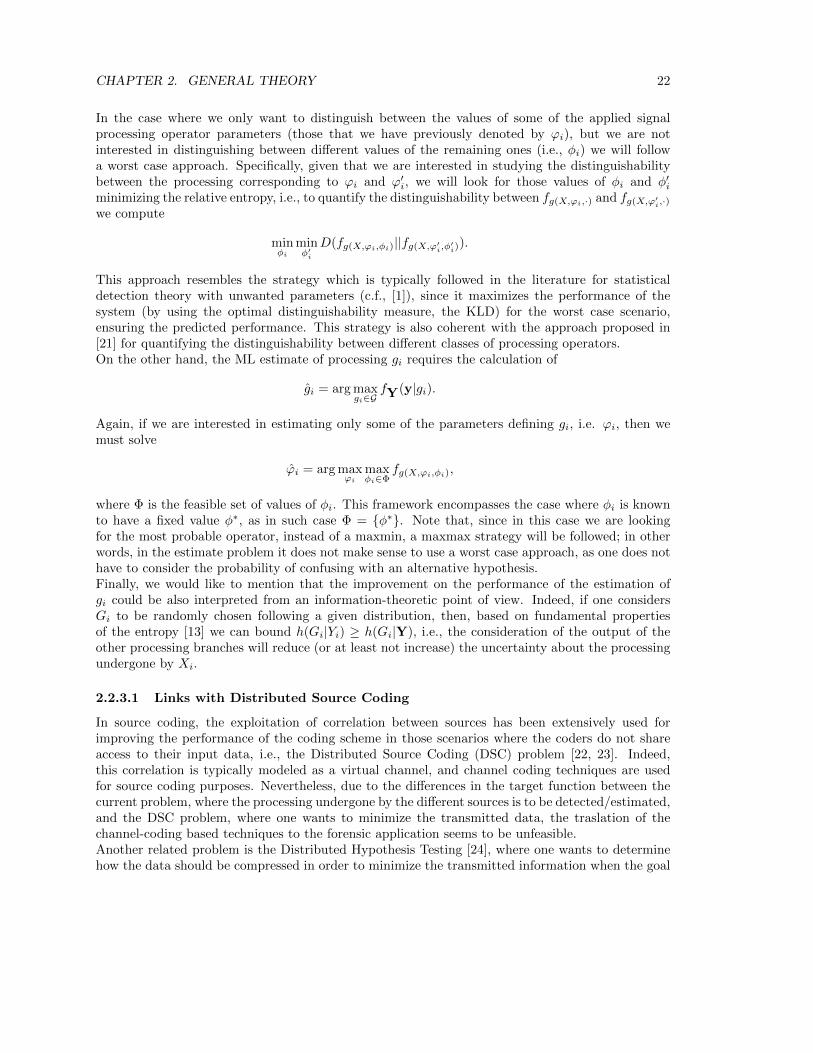
In the case where we only want to distinguish between the values of some of the applied signalprocessing operator parameters (those that we have previously denoted by ϕi), but we are notinterested in distinguishing between different values of the remaining ones (i.e., φi) we will followa worst case approach. Specifically, given that we are interested in studying the distinguishabilitybetween the processing corresponding to ϕi and ϕ′i, we will look for those values of φi and φ′iminimizing the relative entropy, i.e., to quantify the distinguishability between fg(X,ϕi,·) and fg(X,ϕ′i,·)we compute
minφi
minφ′i
D(fg(X,ϕi,φi)||fg(X,ϕ′i,φ′i)).
This approach resembles the strategy which is typically followed in the literature for statisticaldetection theory with unwanted parameters (c.f., [1]), since it maximizes the performance of thesystem (by using the optimal distinguishability measure, the KLD) for the worst case scenario,ensuring the predicted performance. This strategy is also coherent with the approach proposed in[21] for quantifying the distinguishability between different classes of processing operators.On the other hand, the ML estimate of processing gi requires the calculation of
gi = arg maxgi∈G
fY(y|gi).
Again, if we are interested in estimating only some of the parameters defining gi, i.e. ϕi, then wemust solve
ϕi = arg maxϕi
maxφi∈Φ
fg(X,ϕi,φi),
where Φ is the feasible set of values of φi. This framework encompasses the case where φi is knownto have a fixed value φ∗, as in such case Φ = {φ∗}. Note that, since in this case we are lookingfor the most probable operator, instead of a maxmin, a maxmax strategy will be followed; in otherwords, in the estimate problem it does not make sense to use a worst case approach, as one does nothave to consider the probability of confusing with an alternative hypothesis.Finally, we would like to mention that the improvement on the performance of the estimation ofgi could be also interpreted from an information-theoretic point of view. Indeed, if one considersGi to be randomly chosen following a given distribution, then, based on fundamental propertiesof the entropy [13] we can bound h(Gi|Yi) ≥ h(Gi|Y), i.e., the consideration of the output of theother processing branches will reduce (or at least not increase) the uncertainty about the processingundergone by Xi.
2.2.3.1 Links with Distributed Source Coding
In source coding, the exploitation of correlation between sources has been extensively used forimproving the performance of the coding scheme in those scenarios where the coders do not shareaccess to their input data, i.e., the Distributed Source Coding (DSC) problem [22, 23]. Indeed,this correlation is typically modeled as a virtual channel, and channel coding techniques are usedfor source coding purposes. Nevertheless, due to the differences in the target function between thecurrent problem, where the processing undergone by the different sources is to be detected/estimated,and the DSC problem, where one wants to minimize the transmitted data, the traslation of thechannel-coding based techniques to the forensic application seems to be unfeasible.Another related problem is the Distributed Hypothesis Testing [24], where one wants to determinehow the data should be compressed in order to minimize the transmitted information when the goal

CHAPTER 2. GENERAL THEORY 23
is not the reproduction, but the inference from those data. Although in this case we have indeeda detection problem, in the forensic application we are not interested in reducing the transmitteddata; consequently, the traslation of the results in [24] to the current problem appears to be verydifficult.
2.2.4 Gaussian signals and linear operators
In order to provide close formulas that allow a clear comparison between the considered scenarios,we particularize the proposed framework to the case where Gaussian variables and linear processingis considered. Therefore, in this section we will consider the processing defined by Yi = aiXi + Zi,where ai is a real constant, X ∼ N (µX,ΣX), and Zi ∼ N (µZi , σ
2Zi
) is a Gaussian random variableindependent of X and independent of Zj , 1 ≤ j ≤ L, j 6= i. Random variable Zi might modelthe randomness of the processing, for example, the effect of quantizing the processed signal in adifferent domain, e.g., an image operator that scales the 8× 8-block DCT coefficients depending onthe frequency location, and then quantizes the image in the pixel domain; although the quantizationerror is not independent of the DCT coefficients, it is typically modeled as being so (see, for example,[25]), as a lot of different contributions are summed up when performing the DCT and IDCT.Based on the definition of Y, and the distributions of X and Z, Y is also Gaussian, i.e., Y ∼N (µY,ΣY), where
µYi = aiµXi + µZi ,
and (ΣY
)i,j
= aiaj(ΣX
)i,j
+ σ2Ziδ[i− j].
The main advantage of the Gaussian case, that drives us to consider this scenario with special detail,is the fact that closed formulas exist for the KLD of two Gaussian multivariate distributions. Indeed,if we consider Y ∼ N (µY,ΣY) and Y′ ∼ N (µY′ ,ΣY′), then
D(fY||fY′) =1
2
[tr(
Σ−1
Y′ΣY
)+(µY′ − µY
)TΣ−1
Y′(µY′ − µY
)− log
( |ΣY||ΣY′ |
)− L
], (2.24)
where tr(·) is the trace operator, and |Σ| is the determinant of matrix Σ.Taking into account the form of Yi considered in this section, gi is entirely specified by ai andσ2Zi
. In most practical scenarios we will be interested in estimating ai, whereas σ2Zi
is an unwantedparameter; therefore, following the notation introduced in the previous section, ϕi = ai, and φi =σ2Zi
. Consequently, the ML estimate of gain ai requires the calculation of
ai = arg maxai∈R
(maxσ2Zi∈R+
L(y, ai, σ2Zi)
),
where
L(y, ai, σ2Zi) ,
(y − µY
)TΣ−1
Y
(y − µY
)+ log(|ΣY|).
On the other hand, if the unwanted parameter is indeed known a priori, then that knowledge canbe exploited in the estimation. Continuing with the estimate of ai, but assuming that σ2
Ziis known
to be, say,(σ2Zi
)∗, we have that
ai = arg maxai∈R
L(y, ai,(σ2Zi
)∗).

CHAPTER 2. GENERAL THEORY 24
In the following we consider 4 particular scenarios for L = 2 and different definitions of Y2 (Sects. 2.2.4.2-2.2.4.5), while keeping the same definition of Y1. For all of them, we detail the theoretical results ofboth the ML estimator and the KLD. The target of this analysis is to illustrate how the knowledgeof Y2 helps to estimate/detect the processing undergone by Y1 in comparison to the scenario whereonly Y1 is available (Sect. 2.2.4.1). In order to keep the mathematical tractability, we will assumeΣ2Zi
= µXi = µZi = 0, for i = 1, 2. The noisy case (randomized processing operators) and non-zeromean will be considered in Sect. 2.2.5 by numerical results.The proposed scenarios can be linked with real applications in the case of audio stereo files, whereeach audio channel goes through an equalization filter; the samples of each channel are windowed,frequency transformed, and then each frequency coefficient is subjected to a different scaling. Thiseffect can be roughly modeled by a frequency dependent scaling, and the differences between thismodel and the real processing (encompassing, for example, the windowing effect, the lack of blockperiodicity, and the quantization of the filtered samples in the time domain) will be modeled by Zi.Of course the frequency coefficients do not fit the theoretical model studied in this section, but theconsideration of this application scenario showcases the power of the proposed methodology. Wewill particularize this illustrating application for each scenario.
2.2.4.1 Scenario Y1 = a1X1 + Z1
Application Scenario: mono file, or only one of the stereo channels is considered for processingestimation/detection.Under the hypotheses mentioned above,
a1 = ±
√√√√∑Ni=1 (Y i1 )
2
N(ΣX
)1,1
, (2.25)
that is, the variance-based estimator, which in general is biased.Concerning the KLD between Y1 = a1X1 + Z1 and Y ′1 = b1X1 + Z ′1, one obtains
D(fY1||fY ′1 ) =
1
2
(−1 +
a21
b21− log
[a2
1
b21
]). (2.26)
2.2.4.2 Scenario Y1 = a1X1 + Z1, Y2 = a2X2 + Z2, a2 = a1
Application Scenario: stereo case, when we know that the same equalization is applied to bothchannels.The ML estimator can be computed as
a1 = ±
√√√√√∑Ni=1 (Y i1 )
2 (ΣX
)2,2
+ (Y i2 )2 (
ΣX)
1,1− 2 (Y i1Y
i2 )(ΣX
)1,2
2N[(
ΣX)
1,1
(ΣX
)2,2−(ΣX
)21,2
] .
Be aware that whenever X1 and X2 are independent, i.e.,(ΣX
)1,2
= 0, then the derived ML
estimator is
a1 = ±
√√√√ 1
2N
[∑Ni=1 (Y i1 )
2(ΣX
)1,1
+
∑Ni=1 (Y i2 )
2(ΣX
)2,2
], (2.27)
which is obvioulsy related to the ML estimator in (2.25).

CHAPTER 2. GENERAL THEORY 25
Concerning the KLD between (Y1, Y2) = (a1X1 +Z1, a2X2 +Z2) and (Y ′1 , Y′2) = (b1X1 +Z ′1, b2X2 +
Z ′2), we obtain
D(f(Y1,Y2)||f(Y ′1 ,Y′2 )) = −1 +
a21
b21− log
[a2
1
b21
], (2.28)
which is nothing but twice (2.26). This result makes sense, since we are considering the sameprocessing for both channels and the noiseless case, and consequently the correlation between X1
and X2 does not provide any additional information; therefore, from the KLD point of view onewould expect to have the same result that is achieved when two independent realizations of Y1 areavailable. This result also makes sense at the light of (2.27), although in the derivation of the latterwe assumed
(ΣX
)1,2
= 0.
2.2.4.3 Scenario Y1 = a1X1 + Z1, Y2 = a2X2 + Z2. a2 is known
Application Scenario: stereo, we know the equalization applied to one channel, and want toestimate the other one.The ML estimator is
a1 =
{N∑i=1
−a2
(ΣX
)1,2Y i1Y
i2 +
( N∑i=1
a2
(ΣX
)1,2Y i1Y
i2
)2
+ 4Na42
[(ΣX
)1,1
(ΣX
)2,2−(ΣX
)21,2
] (ΣX
)2,2
N∑i=1
(Y i1
)2]1/2
[2Na2
2
((ΣX
)1,1
(ΣX
)2,2−(ΣX
)21,2
)]−1
. (2.29)
Concerning the KLD between (Y1, Y2) = (a1X1 +Z1, a2X2 +Z2) and (Y ′1 , Y′2) = (b1X1 +Z ′1, b2X2 +
Z ′2), we obtain
D(f(Y1,Y2)||f(Y ′1 ,Y′2)) =− 1− 1
2log
(a2
1a22
b21b22
)+
(a2
2b21 + a2
1b22
) (ΣX
)1,1
(ΣX
)2,2− 2a1a2b1b2
(ΣX
)21,2
2b21b22
[(ΣX
)1,1
(ΣX
)2,2−(ΣX
)21,2
] . (2.30)
Note that whenever(ΣX
)1,2
= 0
D(f(Y1,Y2)||f(Y ′1 ,Y′2 )) = 1
2
[−1 +
a21
b21− log
(a2
1
b21
)− 1 +
a22
b22− log
(a2
2
b22
)],
which also follows the intuition for the KLD of multivariate Gaussian distributions of diagonalcovariance matrices.The scenario Y1 = a1X1 +Z1, Y2 = a2X2 +a3X1 +Z2 (so Y2 6= g2(X2)), where a2 and a3 are known,was also studied, although the obtained results are not shown here due to spatial constraints. Letonly mention that it corresponds to the stereo case, where channel 2 is not only equalized, but editedby combining it with a filtered version of channel 1. Our target would be to estimate the equalizerundergone by output 1, that depends only on channel 1 input.

CHAPTER 2. GENERAL THEORY 26
2.2.4.4 Scenario Y1 = a1X1 + Z1, Y2 = a2X2 + Z2. a2 is not known
Application Scenario: stereo, we want to estimate the equalizer applied to one of the channels,but we do not know about the equalization applied to the other one.In this framework, the value of a2 (as a function of a1) maximizing the ML target function is
−ξ+
√ξ2+4Na1
[(ΣX
)1,1
(ΣX
)2,2−(ΣX
)2
1,2
]∑Ni=1 a1
(ΣX
)1,1
(Y i2 )2
2Na1
[(ΣX
)1,1
(ΣX
)2,2−(ΣX
)2
1,2
] ,
where ξ ,∑Ni=1
(ΣX
)1,2Y i1Y
i2 , yielding the ML estimator
a1 = ±
√√√√√√√(ΣX
)2,2κ−
√(ΣX
)2,2(
ΣX)
1,1
(ΣX
)21,2κ[∑N
i=1 Yi1Y
i2
]2N[(
ΣX)
1,1
(ΣX
)2,2−(ΣX
)21,2
]∑Ni=1 (Y i2 )
2,
where κ ,[∑N
i=1
(Y i1)2] [∑N
i=1
(Y i2)2]
. Note that whenever(ΣX
)1,2
= 0, then this estimator is
equivalent to (2.25).On the other hand, in the computation of the KLD, and given that we study the distinguishabilitybetween the processing corresponding to a1 and b1, we will look for those values of a2 and b2minimizing the KLD. In the current scenario, the derivative of the KLD with respect to a2 is
− 1
a2+b1a2
(ΣX
)1,1
(ΣX
)2,2− a1b2
(ΣX
)21,2
b1b22
[(ΣX
)1,1
(ΣX
)2,2−(ΣX
)21,2
] ,
which has roots with respect to a2 atb2
(a1
(ΣX
)2
1,2+γ
)2b1(
ΣX)
1,1
(ΣX
)2,2
, where γ ,
√a21
(ΣX
)41,2 + 4b21
(ΣX
)1,1
(ΣX
)2,2
[(ΣX
)1,1
(ΣX
)2,2 −
(ΣX
)21,2
].
If one replaces (2.2.4.4) into the relative entropy, the result does not depend on b2, so the minimiza-tion over that variable is indeed not necessary. The obtained value is
D(f(Y1,Y2)||f(Y ′1 ,Y′2 )) =− 1
2
+a2
1
[2(ΣX
)21,1
(ΣX
)22,2−(ΣX
)41,2
]− a1
(ΣX
)21,2κ
4b21(ΣX
)1,1
(ΣX
)2,2
[(ΣX
)1,1
(ΣX
)2,2−(ΣX
)21,2
]− 1
2log
a21
[a1
(ΣX
)21,2
+ κ]2
4b41(ΣX
)21,1
(ΣX
)22,2
.
An interesting scenario, is that where(ΣX
)1,2
= 0; under that assumption, the derivative of the
KLD with respect to a2 is equal to − 1a2
+ a2
b22, yielding the condition a2
2 = b22. Indeed, in that
particular framework the KLD can be written as (check the obvious relationships with (2.26))
D(f(Y1,Y2)||f(Y ′1 ,Y′2 )) =
1
2
(−1 +
a21
b21− log
[a2
1
b21
])+
1
2
(−1 +
a22
b22− log
[a2
2
b22
]),

CHAPTER 2. GENERAL THEORY 27
and consequently we can minimize the KLD overa2
2
b22; straightforwardly, the achieved solution is
a22
b22= 1, providing a null contribution to the total KLD, whose value will be
D(f(Y1,Y2)||f(Y ′1 ,Y′2 )) =
1
2
(−1 +
a21
b21− log
[a2
1
b21
]), (2.31)
i.e., the same value achieved in (2.26). The implications of this result are evident:
• Since X1 and X2 are independent, the consideration of Y2 and Y ′2 will not provide any knowl-edge that can improve the distinguishability between a1 and b1.
• Therefore, if we look for those values of a2 and b2 minimizing the KLD, we will find thata2
2 = b22 (due to the symmetry obtained by assuming zero-mean random variables).
• Consequently, we go back to the framework studied in Sect. 2.2.4.1.
Another asymptotical scenario, that is also particularly interesting, is that where(ΣX
)1,2→
±√(
ΣX)
1,1
(ΣX
)2,2
, i.e., if X1 and X2 are (almost) deterministically related. It can be checked
that in that framework the KLD goes to infinity whenever a2 6= a1b2b1
. The intuition behind this
result is also interesting: since X1 and X2 are related by a fixed factor, if we compute Y1
Y2= a1
a2it
will be trivial to distinguish that scenario fromY ′1Y ′2
= b1b2
unless a1
a2= b1
b2.7
Therefore, in order to follow our worst case approach, we will choose a2 to be a1b2b1
. By doing so,the resulting KLD value is
D(f(Y1,Y2)||f(Y ′1 ,Y′2 )) = −1 +
a21
b21− log
[a2
1
b21
],
which is nothing but twice (2.26) (and therefore twice (2.31)), and exactly the same than (2.28),although in that case this value was obtained for a generic covariance matrix.Again, this result illustrates what one would intuitively expect; the larger the correlation betweenthe sources, the easier it will be to distinguish between the operators. Indeed, the two limit behaviorsare also very enlightening:
• Whenever the considered sources are independent, the achieved KLD is equivalent to thatwhere only Y1 is considered. Of course in this framework Y2 does not provide any knowledgeon Y1, and consequently we can just neglect that variable.
• Whenever the relationship between the sources is deterministic, the problem is equivalent tohaving two independent observations, coming from a single source.
2.2.4.5 Scenario Y1 = a1X1 + Z1, Y2 = a2X2 + a3X1 + Z2, so Y2 6= g2(X2). a2 and a3 areknown.
Application Scenario: stereo, channel 2 is not only equalized, but edited by combining it with afiltered version of channel 1. We want to estimate the equalizer undergone by output 1, that dependsonly on channel 1 input.
7Take into account that we assume this equality to hold before taking the limit(ΣX
)1,2→ ±
√(ΣX
)1,1
(ΣX
)2,2
.
In the limit the covariance matrix of X becomes singular (with computational problems arising when computing
(2.24)), so it is important to note that by considering a1a2
= b1b2
the KLD does not depend on the covariance matrix of
X.
CHAPTER 2. GENERAL THEORY 28
The ML estimator is
a1 =
∑Ni=1
[−(a3
(ΣX
)1,1
+ a2
(ΣX
)1,2
)Y i1Y
i2
]2Na2
[a2
(ΣX
)1,1
(ΣX
)2,2− 2a3
(ΣX
)1,1
(ΣX
)1,2− a2
(ΣX
)21,2
]+
( N∑i=1
(a3
(ΣX
)1,1
+ a2
(ΣX
)1,2
)Y i1Y
i2
)2
+4Na2
[a2
(ΣX
)1,1
(ΣX
)2,2− 2a3
(ΣX
)1,1
(ΣX
)1,2− a2
(ΣX
)21,2
]N∑i=1
[(a2
3
(ΣX
)1,1
+ a22
(ΣX
)2,2
)Y 2
1
]]{
2Na2
[a2
(ΣX
)1,1
(ΣX
)2,2− 2a3
(ΣX
)1,1
(ΣX
)1,2− a2
(ΣX
)21,2
]}−1
.
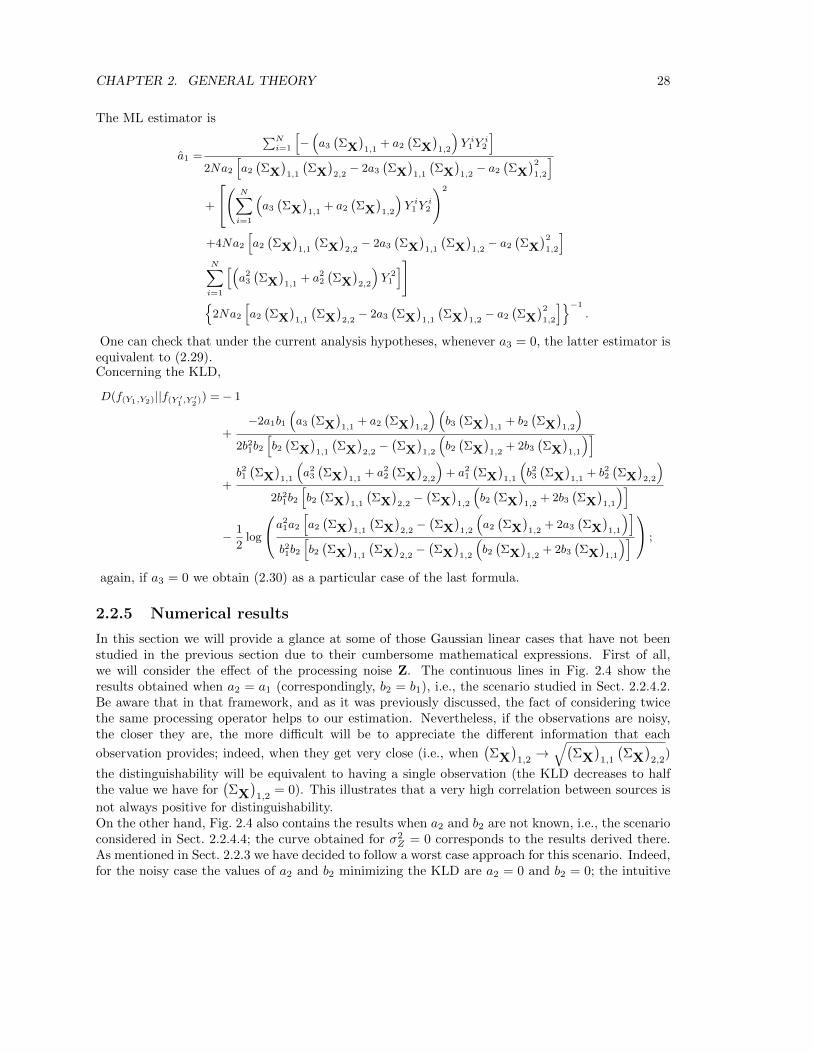
One can check that under the current analysis hypotheses, whenever a3 = 0, the latter estimator isequivalent to (2.29).Concerning the KLD,
D(f(Y1,Y2)||f(Y ′1 ,Y′2)) =− 1
+−2a1b1
(a3
(ΣX
)1,1
+ a2
(ΣX
)1,2
)(b3(ΣX
)1,1
+ b2(ΣX
)1,2
)2b21b2
[b2(ΣX
)1,1
(ΣX
)2,2−(ΣX
)1,2
(b2(ΣX
)1,2
+ 2b3(ΣX
)1,1
)]+b21(ΣX
)1,1
(a2
3
(ΣX
)1,1
+ a22
(ΣX
)2,2
)+ a2
1
(ΣX
)1,1
(b23(ΣX
)1,1
+ b22(ΣX
)2,2
)2b21b2
[b2(ΣX
)1,1
(ΣX
)2,2−(ΣX
)1,2
(b2(ΣX
)1,2
+ 2b3(ΣX
)1,1
)]− 1
2log
a21a2
[a2
(ΣX
)1,1
(ΣX
)2,2−(ΣX
)1,2
(a2
(ΣX
)1,2
+ 2a3
(ΣX
)1,1
)]b21b2
[b2(ΣX
)1,1
(ΣX
)2,2−(ΣX
)1,2
(b2(ΣX
)1,2
+ 2b3(ΣX
)1,1
)] ;
again, if a3 = 0 we obtain (2.30) as a particular case of the last formula.
2.2.5 Numerical results
In this section we will provide a glance at some of those Gaussian linear cases that have not beenstudied in the previous section due to their cumbersome mathematical expressions. First of all,we will consider the effect of the processing noise Z. The continuous lines in Fig. 2.4 show theresults obtained when a2 = a1 (correspondingly, b2 = b1), i.e., the scenario studied in Sect. 2.2.4.2.Be aware that in that framework, and as it was previously discussed, the fact of considering twicethe same processing operator helps to our estimation. Nevertheless, if the observations are noisy,the closer they are, the more difficult will be to appreciate the different information that each
observation provides; indeed, when they get very close (i.e., when(ΣX
)1,2→√(
ΣX)
1,1
(ΣX
)2,2
)
the distinguishability will be equivalent to having a single observation (the KLD decreases to halfthe value we have for
(ΣX
)1,2
= 0). This illustrates that a very high correlation between sources is
not always positive for distinguishability.On the other hand, Fig. 2.4 also contains the results when a2 and b2 are not known, i.e., the scenarioconsidered in Sect. 2.2.4.4; the curve obtained for σ2
Z = 0 corresponds to the results derived there.As mentioned in Sect. 2.2.3 we have decided to follow a worst case approach for this scenario. Indeed,for the noisy case the values of a2 and b2 minimizing the KLD are a2 = 0 and b2 = 0; the intuitive

CHAPTER 2. GENERAL THEORY 29
0 0.5 1 1.5 2 2.50.025
0.03
0.035
0.04
0.045
0.05
0.055
0.06
(ΣX)1,2
D(f
1||f2)
σZ2 = 0
σZ2 = 10−3
σZ2 = 10−2
σZ2 = 10−1
Figure 2.4: KLD when a2 = a1 and b2 = b1 (continuous lines) and when a2 and b2 are not known(discontinuous ones), for different values of σ2
Z1= σ2
Z2= σ2
Z . a1 = 1, b1 = 1.2,(ΣX
)1,1
= 2,(ΣX
)1,1
= 3,(ΣX
)1,2∈[0,√(
ΣX)
1,1
(ΣX
)2,2
], µX = 0, µZ = 0.
0 0.5 1 1.5 2 2.50.02
0.04
0.06
0.08
0.1
0.12
0.14
0.16
0.18
0.2
(ΣX)1,2
D(f
1||f2)
µX = 3
µX = 2
µX = 1
µX = 0
Figure 2.5: KLD when a2 and b2 are not known, for σ2Z1
= σ2Z2
= 0 and different values of µX1=
µX2= µX . a1 = 1, b1 = 1.2,
(ΣX
)1,1
= 2,(ΣX
)1,1
= 3,(ΣX
)1,2∈[0,√(
ΣX)
1,1
(ΣX
)2,2
],
µZ = 0.
idea behind this result is also clear: in the worst case we cannot trust the second observation, as itis only noise. In that case the KLD is
1
2
[a2
1
(ΣX
)1,1
+ σ2Z
b21(ΣX
)1,1
+ σ2Z
− log
(a2
1
(ΣX
)1,1
+ σ2Z
b21(ΣX
)1,1
+ σ2Z
)− 1
],
which is independent of the correlation term, as expected.Finally, the influence of the mean of the original signal on the distinguishability is illustrated inFig. 2.5, which clearly shows that the larger the mean of the signal, the easier will be to distinguishthe considered processing operators.
2.2.6 Conclusions
In this work we have quantified the advantages of using the joint distribution of composite objects forimproving the distinguishability between processing operators. Although for the sake of tractability

CHAPTER 2. GENERAL THEORY 30
we have focused on the linear Gaussian case, it is evident that the principles derived here wouldbe applicable to more general frameworks. Among these principles, we can mention the behaviorof the distinguishability measures in different scenarios, and how, for example, the case where thecorrelated sources are known to share their processing is equivalent to having independent sources.It also interesting to note that for the case where the unwanted processing is unknown, for thenoiseless case the distinguishability achieved for deterministically correlated sources is double theone obtained for independent sources, but for the noisy case the obtained value is independent ofthat correlation, as the second observation is considered to be pure noise. Finally, we would liketo mention the a priori striking result showing that a larger correlation between sources does notalways imply a better distinguishability between operators.

Chapter 3
Operator chain modeling
3.1 JPEG Quantization and full-frame filtering
A plethora of forensics techniques have been proposed in the literature so far, aiming at identifyingspecific processing operators applied to images [26], but little attention has been paid on the forensicanalysis of chains of operators. In such a scenario, difficulties in the detection may arise since thestatistical footprints exploited to detect a specific processing may be wiped off by the application ofa second one. We propose here to continue and extend our previous work, where we analyzed theDiscrete Cosine Transform (DCT) statistical properties of a JPEG image, post-processed with linearprocessing operators. In this scenario, some well-known statistical properties of a JPEG image areperturbed, thus complicating the application of previous forensic works (e.g. [25],[27]). We derivean accurate mathematical model that establishes a precise relationship between DCT coefficientsbefore and after filtering. Finally, the presented analysis is exploited to build a model for the DCTdistribution of JPEG images filtered with various linear kernels. We will assume in this work thequantization to be fixed and known, although future work will be devoted to remove this assumption.By mean of the χ2 histogram distance, we measure the distinguishability between the derived models(each model depends on the applied filter kernel) and the actual distribution of a to-be-tested image,aiming at identifying the linear operator which has been applied. Other distinguishability measuresmay be employed. The choice of χ2 distance was primarily due to the widespread use of the χ2
goodness of fit test (also known as Pearsons test [28]) as one of the most accepted non-parametricstatistical test for determining if an observed frequency distribution matches with a theoreticalone or not. It has been successfully employed in many research areas, e.g., near duplicate imageidentification [29], shape and texture classification [30] and steganography [31]. Moreover, in [32] ithas been shown that out of a number of non-parametric test statistics, χ2 metric gets some of thebest results in terms of accurate distance metric for probability density functions.To the best of our knowledge, the presented work constitutes a first attempt to study the statisticalperturbation introduced by linear operators on JPEG images and, although their detection is notnecessarily proof of malicious tampering, the derived framework represents a valuable mean todisclose the processing history.In Section 3.1.1 we briefly review the needed mathematical background, while in Section 3.1.2 werecall our previous work on the definition of the mathematical model characterizing the statisticalproperties of a JPEG linearly filtered image. Following, in Section 3.1.3 we present the experimentaltests we carried out in order to verify the efficacy of the proposed method. We collect some conclusionand describe some still open issues to be further investigated in Section 3.1.4.
31

CHAPTER 3. OPERATOR CHAIN MODELING 32
3.1.1 Block-wise JPEG compression and full-frame linear filtering
The JPEG standard provides a block-based compression scheme, which operates on 8 × 8 non-overlapping blocks of DCT coefficients. In its most commonly used format, it is well known tobe a lossy scheme, i.e., some information is lost during the process, mainly due to a quantizationoperation.In particular, an image I of size (Mx×My), here just considering the luminance channel for simplicity,is firstly partitioned into (Bx ×By) non-overlapping blocks of size 8× 8. Each block (bx, by) is thenindependently transformed from the spatial to the frequency domain, using the DCT:
d(bx,by)(i, j) =c(i)
2
c(j)
2
7∑n1=0
7∑n2=0
o(bx,by)(n1, n2) cos
(2n1 + 1
16πi
)cos
(2n2 + 1
16πj
), (3.1)
where d(bxby)(i, j) is the frequency coefficient at position (i, j) in the (bxby)-th block, with (i, j) ∈{0, . . . , 7}2, and o(bxby)(n1, n2) is the pixel at position (n1, n2) in the (bxby)-th block of the inputimage. Moreover, c(s) = 1 if s > 0, and c(s) = 1/
√2 if s = 0.
Depending on the compression quality, a specific 8 × 8 quantization table is employed to quantizeeach DCT frequency:
d(bx,by)q (i, j) = round
(d(bx,by)(i, j)
∆(i, j)
),
where ∆(i, j) are the quantization steps associated with each frequency (i, j). Such quantized co-efficients are finally entropy-encoded (Huffman coding) and stored in the JPEG file format. Thecompressed data stream can be decompressed, applying all the steps in reverse order. Specifically,a DCT coefficient is reconstructed as
d(bx,by)q (i, j) = ∆(i, j) · round
(d(bx,by)(i, j)
∆(i, j)
), (3.2)
and is finally transformed from the frequency to the spatial domain by applying the Inverse DCTon each 8× 8 block:
J (bx,by)(i, j) =
7∑k1=0
7∑k2=0
c(k1)
2
c(k2)
2d(bx,by)q (k1, k2) cos
(2i+ 1
16πk1
)cos
(2j + 1
16πk2
), (3.3)
where J (bx,by)(i, j) is the pixel value at position (i, j) in the (bx, by)-th block of the JPEG image.From (3.2), the de-quantized coefficients are mapped to multiples of the quantization step ∆(i, j),resulting in specific artifacts in the coefficient distribution. Fig. 3.1(a) shows the histogram of theDCT coefficients at frequency (1, 2) collected from a subset of 669 un-compressed images [33], whileFig. 3.1(b) depicts the distribution of the same data after quantization, with ∆(1, 2) = 10. Itbecomes clear that the structure of such histogram is related to the employed quantization factor.For the sake of presentation we disregard the round-off and truncation errors, in the pixel domain,introduced by the compression scheme, without affecting the conducted analysis. Previous works inthe literature demonstrate that, by exploiting the described artifacts in the distribution, it is possibleto discover instances of previous JPEG compression and even estimate the used quantization steps[25, 27, 34, 35]. However, it is very likely that later in its life the JPEG-compressed image willbe processed by a further operator to enhance its quality. For example, it is frequent the useof full-frame operators aimed at reducing the JPEG-compression block effects. By doing so, the

CHAPTER 3. OPERATOR CHAIN MODELING 33
−50 −40 −30 −20 −10 0 10 20 30 40 500
0.05
0.1
0.15
0.2
0.25
0.3
(a)
(b)
−50 −40 −30 −20 −10 0 10 20 30 40 500
0.01
0.02
0.03
0.04
0.05
0.06
0.07
0.08
0.09
0.1
−50 −40 −30 −20 −10 0 10 20 30 40 500
0.01
0.02
0.03
0.04
0.05
(c)
Figure 3.1: Panel (a) shows the original DCT histogram for frequency (1, 2) collected from a subset of669 uncompressed images and its curve fitting. In panel (b), the same distribution after quantization with∆(1, 2) = 10 is presented. Panel (c) shows the given distribution when a linear filtering operator (an averagefilter of size 3×3) has been further applied, together with the derived model for such distribution (red line).
characteristic artifacts present in the DCT distribution of JPEG images may be partially perturbed,making harder the application of those forensic algorithms. In this work, we study the combinationof JPEG compression and full-frame linear filtering operations. Up to now, very little attentionhas been paid to study such a scenario. Specifically, linear filtering represents an interesting casestudy since it is a very common and useful linear tool applied for image enhancement, such as edgesharpening, noise removal illumination correcting and deblurring. It operates by convolving theoriginal image with an appropriate filter kernel. The result of such a convolution is a filtered image,whose pixel values are a weighted sum of a certain number of neighboring pixels:
F (x, y) =
N∑s1=−N
N∑s2=−N
h(s1, s2)J(x+ s1, y + s2),
where J(x, y) , J (bx,by)(i, j), i = xmod8, j = ymod8, bx = dx8 e, by = dy8 e, x ∈ {0, ...,Mx − 1}and y ∈ {0, ...,My − 1}, and h is the filter kernel of size (2N + 1) × (2N + 1). Fig. 3.1(c) showsthe histogram of the DCT frequency coefficients of panel (b) after filtering with an Average 3 × 3

CHAPTER 3. OPERATOR CHAIN MODELING 34
filter; the characteristics of the histogram of the quantized coefficients are clearly perturbed, butnew patterns appear, depending both on the employed quantization factor and the filter kernel.The aim of this research is to study such artifacts in order to identify the filter kernel a JPEGimage has undergone. In order to do this, we mathematically analyze the DCT distribution ofcompressed and filtered images and derive an accurate model for them. Specifically, we investigatethe statistical characteristics in the distribution of the DCT coefficients and, as a first result of thatanalysis, show that the extended assumption about the image AC DCT coefficients for differentfrequencies being independent, and for the same frequency being i.i.d. [36][37], does not hold;indeed, the inter- and intra-block redundancy of the quantized DCT coefficients must be taken intoaccount. By considering those redundancies on the provided analysis, the studied processing can beaccurately modeled and a general mathematical model for the distributions of DCT coefficients ofJPEG filtered images can be derived, depending on the applied kernel and assuming the quantizationto be fixed and known. Fig. 3.1(c) serves as an example of the derived model for the probabilitydistribution of JPEG filtered images. Later, we build a dictionary-based database for the derivedmodels corresponding to different applied filters and a distinguishability measure is calculated toquantify the difference between the theoretically derived models and the actual distribution of animage. In this analysis, we employ the χ2 histogram distance, which comes from the χ2 test [38],commonly used to compare observed frequencies with a theoretical distribution (e.g., it has beensuccessfully used in steganography to detect if some embedding has taken place [31]). For discretesignals, the χ2 distance is defined as follows:
χ2 =1
2
∑i
(Pi −Qi)2
(Pi +Qi), (3.4)
where P and Q are two probability distributions to be compared. Intuitively, the χ2 distance wouldtend to zero when the two distributions are very close. So, in our scheme, a lower χ2 measure willbe an evidence that will allow to identify the filter operator applied to the under-test image.
3.1.2 Mathematical model
We derive a theoretical model to describe the statistical properties of an image that has been firstJPEG compressed and then linearly filtered. In order to do that, we mathematically express thedeterministic relation between the quantized DCT coefficient dq(x, y) and that of the JPEG andfiltered image df (x, y). Then, by exploiting the knowledge about the statistical properties of the
distribution of dq(x, y), we further analyze the histograms of df (x, y), assess the dependency of thedifferent frequencies and derive a model to theoretically characterize the probability distribution ofthe DCT coefficients of a JPEG image filtered with a given filter kernel.The study case here concerned is shown in Fig. 3.2. Following the scheme backwards, we startconsidering the DCT coefficients df (x, y) of a JPEG compressed and filtered image and, accordingto (3.1), transform them into the spatial domain F (x, y). Through a linear convolution operationwith the filter kernel h, we can further express df (x, y) as a function of the pixels of the compressed
image J , which represents the Inverse DCT of dq(x, y) (3.3). Exploiting the linearity property ofboth the filtering operation and the DCT transform, we are able to mathematically formulate therelation between the DCT coefficients of a quantized image dq(·, ·) and the DCT coefficients of thefurther filtered image df (·, ·). Specifically, given a filter kernel of size smaller than or equal to 17,
the coefficients dq(x, y) contributing in the calculation of df (x, y) are those from the same block ofdf (x, y) plus those from the 8 immediate surrounding blocks, resulting in 24 × 24 coefficients. Itbecomes clear that for filter kernels of sizes larger than 17, the number of contributing coefficients

CHAPTER 3. OPERATOR CHAIN MODELING 35
DCT IDCT LINEAR FILTER DCT
JPEG IMAGE DCT domain
JPEG IMAGE SPATIAL domain
JPEG FILTERED IMAGE
SPATIAL domain
JPEG FILTERED IMAGE
DCT domain
dq(x, y) F (x, y)J(x, y)J(x, y) df (x, y)
JPEG IMAGE SPATIAL domain
h
Figure 3.2: Block scheme of the considered processing operations. The aim is to establish a math-ematical relationship between the quantized DCT coefficient dq(x, y) and that of the JPEG and
filtered image df (x, y) in order to exploit the statistical properties of the distribution of dq(x, y).
df (x, y) =DCTα,β
([h ∗ IDCTα,β
(dq(x, y)
)]b x8 c+7,b y8 c+7
b x8 c,by8 c
)+
∑(k1,k2)∈{−8,...,15}2,(k1,k2)6=(α,β)
DCTα,β
([h ∗ IDCTα′,β′
(dq
(⌊x8
⌋+ k1,
⌊y8
⌋+ k2
))]b x8 c−b k18 c+7,b y8 c−b
k28 c+7
b x8 c−bk18 c,b
y8 c−b
k28 c
).
(3.6)
would increase, involving more surrounding blocks. In Section 3.1.2.1, we will show that only asubset of all the DCT coefficients is effectively relevant for the computation of each coefficientdf (x, y). Finally, we make explicit the contribution of the DCT coefficient dq(x, y) at the sameposition of df (x, y), as follows:
df (x, y) = γ · dq(x, y) +N, (3.5)
where γ,N ∈ R are a scaling factor and a noise term, respectively. These two terms can be calculated,through some math, according to (3.6), where α = xmod8, β = ymod8, α′ = k1mod8, β′ = k2mod8,DCTx,y is the (x, y)-th DCT coefficient obtained from an 8×8 pixel block, IDCTx,y is the 8×8 pixelblock (located at {bx8 c, . . . , bx8 c + 7} × {by8 c, . . . , b
y8 c + 7}) obtained by applying the IDCT to the
(x, y) DCT coefficient, ∗ denotes the bidimensional convolution, and [A]c,da,b denotes the submatrixof an arbitrary matrix A with first index taking values in {a, . . . , b}, and second index in {c, . . . , d}.N stands for the second term in the summation in (3.6).
3.1.2.1 Probability distribution
Once we have derived the deterministic expression in (3.5) for df (x, y), we can exploit the knowledge
about the distribution of the quantized coefficients dq(x, y) to analyze the distribution of the DCTcoefficients of the final image F .Usually, the probability distribution of DCT coefficients in natural images is modeled as a zero-mean

CHAPTER 3. OPERATOR CHAIN MODELING 36
Generalized Gaussian (Fig. 3.1(a)):
fGGD(d(i, j)) =s
2aΓ(1/s)exp− (|t|/a)s, (3.7)
where Γ denotes the gamma function, a and s are the scale and the shape parameter, respectively.Due to quantization, the probability distribution of each quantized DCT coefficient will be [25](Fig. 3.1(b))
Lλ(k∆) ,f(dq(i, j) = k∆|∆)=
∫ (k+ 12 )∆
(k− 12 )∆
fGGD(τ)dτ, (3.8)
where k ∈ Z and, for the sake of notation simplicity, ∆ = ∆(i, j). Therefore the probability massfunction of each frequency coefficient of a JPEG image is
f(dq(i, j) = τ |∆) =∑k
δ(τ − k∆)Lλ(k∆). (3.9)
It becomes clear that the distribution of (3.9) presents specific artifacts, whose structure is relatedto the quantization step. In particular, the DCT coefficients corresponding to the (i, j)-th frequencywill be located at multiples of the applied quantization step ∆(i, j), as illustrated in Fig. 3.1(b).From probability theory [39], given two discrete independent random variables, the probability den-sity function (pdf) of their sum is the convolution of their corresponding pdfs. Therefore, accordingto the derived mathematical model in (3.5), and based on the common DCT coefficients models,which typically assume the different frequency components to be independent and the coefficientsin a given frequency to be i.i.d. [40], we would expect the probability distribution of the DCT coef-ficients df (x, y) to be the result of a convolution between a train of impulses located at γ · k∆(i, j),with γ ∈ R and k ∈ Z, and a noise component due to the contributions of all the neighboringcoefficients (3.5). Moreover, we will model the noise components as a GGD distributed variable,according to (3.7), with GGD parameters depending on each centroid γ · k∆(·, ·) about which suchnoise is centered.However, we will illustrate that indeed the typical assumptions on the DCT coefficients distributionof natural images do not hold, thus resulting in a deviation between the classical theoretical modelsand the empirical data. Specifically, a scaling between the peaks in the histogram of the DCTcoefficients of the compressed and filtered image and the impulse train identifying the location ofthe translated quantization step γ · k∆(·, ·) is observed. This suggests the need for a differentmodel for the noise component in (3.5), which cannot any longer be considered as the addition ofindependent variables (coefficients of different frequencies) and i.i.d. components (coefficients in thesame frequency). Therefore, we analyze the mean of the noise component and verify that for realimages it monotonically increases with the quantized samples value. As an example, in Fig. 3.3 thered curve represents the mean of the noise component when a Moving Average filter of size 3 × 3is applied, plotted with respect to each translated quantized value γ · k∆(i, j); similar behaviorshave been verified for different filter kernels. Moreover, for each coefficient df (x, y), we isolate thecontribution of each 24× 24 coefficient and analyze their influence. In Fig. 3.3 (a)-(b) we show thespecific pattern of coefficients mainly contributing to the noise, for all the AC coefficients (1, 2) and(2, 1). The red curve represents the mean of the total noise component over γ · k∆(·, ·), the bluecurve represents the contribution of a specific set of coefficients and the black curve correspondsto the contribution of all the remaining coefficients not specified in the previous set. This set wasdetermined by isolating those coefficients that provided a significant noise contribution, in absolutevalue, over all γ ·k∆(·, ·) (i.e., above an empirically determined threshold.) Note that the 24×24 grid

CHAPTER 3. OPERATOR CHAIN MODELING 37
(a)
−40 −30 −20 −10 0 10 20 30 40−20
−15
−10
−5
0
5
10
15
20Coeff: (1,2)
a kq(1,2)
mea
n No
ise
TotalIndexOthers
x
� · k�(1, 2)
(b)
−40 −30 −20 −10 0 10 20 30 40−20
−15
−10
−5
0
5
10
15
20Coeff: (2,1)
a kq(2,1)
mea
n No
ise
TotalIndexOthers
x
� · k�(2, 1)
Figure 3.3: Inter- and intra-block spatial redundancy affecting to df (x, y), over the entire image database.In each panel, corresponding to the frequencies (1, 2) and (2, 1), respectively (black cross in the grid in theupper left of each subplots), the total mean of the noise component (red curve) is plotted with respect tothe values of the quantized filtered coefficients γ · k∆q(i, j). The blue curve represents the contribution ofa set of coefficients (depicted in blue in the grid) and the black curve corresponds to the contribution of allthe remaining coefficients not specified in the previous set.
in the upper left part of each plot corresponds to the 9 DCT blocks taken into account in (3.5), whenemploying a kernel filter of size smaller than or equal to 17. The black dot identifies the consideredfrequency and the blue dots correspond to set of coefficients which mainly influence the total noise,as verified by the curve matching. Note that due to space restrictions, we report only the behaviorfor the coefficients (1, 2) and (2, 1), but the 8 lowest frequencies in an 8× 8 DCT block, discardinghigher frequencies which are more likely to be quantized to zero, have been analyzed giving similarresults.Therefore, an accurate model for the distribution of the DCT coefficients of a filtered JPEG imagecan be derived, taking into account the scaling inferred by the noise component. In Fig. 3.4 it isshown how the translated impulses, now centered in γ ·k∆(·, ·) plus the mean of the noise component,match with the peaks of the histogram.

CHAPTER 3. OPERATOR CHAIN MODELING 38
−40 −30 −20 −10 0 10 20 30 400
0.1
0.2
0.3
0.4
0.5
0.6
0.7
0.8
0.9
1
Filtered dcta kq(1,2)a kq(1,2)+meanNoise� · k�(1, 2)
� · k�(1, 2) + meanNoise
Filtered dct
Figure 3.4: Probability distribution, at frequency (1, 2), quantized with a step q(1, 2) = 10 and filtered witha 3 × 3 averaging filter. The red impulses represent the location of γ · k∆(1, 2) while the yellow ones aretranslated by the mean of the Noise component. The latter perfectly match with location of the peaks inthe histogram.
3.1.3 Proposed forensic approach
The main idea of the proposed forensic approach is to estimate the filter operator an image has beengone through. We note that linear filtering is a very powerful tool employed for image enhancement.As a first attempt in this forensic case study, we assume the quantization applied to the image duringcompression to be known a priori. Future work will release this assumption. The main idea is tomodel the probability distributions of the DCT coefficients of an image being filtered with one ofthe linear filters present in a predefined dictionary.To build a generalized model associated with each filter in the dictionary, we proceed as follows:
• We collect the (1, 2), (2, 1) and (2, 2) DCT frequency coefficients from a random half of the 1338images present in the UCID- Uncompressed Image Database [33]. We then fit, for each fre-quency, a Generalized Gaussian distribution, as in (3.7). This fitting is as shown in Fig. 3.1(a).
• We evaluate the distribution of the quantized coefficients, according to (3.8). In this work wesimulated a uniform scalar quantizer with step size ∆ = 10 (Fig. 3.1(b)).
• We select a set of linear filters to be part of the dictionary, among which, Moving Average,Gaussian, Laplacian, with different settings for the window size, the variance σ2 or the scaleparameter α, as reported in Tab. 3.1.
• For each filter and AC DCT coefficient, we calculate γ in (3.5), according to (3.6).
• For each γ · k∆(·, ·) the corresponding noise component is modeled as a GGD.
• The distribution of DCT coefficients, quantized and filtered with a given kernel, will be thesum of many GGDs, each of them centered in γ · k∆(·, ·) translated by the mean of the noisecomponent and with amplitude depending on the distribution of the quantized and not filteredcoefficients, i.e., (3.8).
An example of the generalized model for the average filter with window size 3 × 3 is reported inFig. 3.1(c).

CHAPTER 3. OPERATOR CHAIN MODELING 39
1. LP Average [3× 3] 3. LP Gaussian [3 × 3],σ2= 0.5
9. LP Laplacian, σ2=0.2
2. LP Average [5× 5] 5. LP Gaussian [3 × 3],σ2= 0.5
10. LP Laplacian, σ2=0.7
4. LP Gaussian [3 × 3],σ2= 1
7. HP Laplacian, σ2= 0.2 11. HP Average [3× 3]
6. LP Gaussian [5 × 5],σ2= 1
8. HP Laplacian, σ2= 0.7 12. HP Average [5× 5]
Table 3.1: Filters selected to be part of the dictionary-based filter database, grouped according tothe similarity of their frequency response.
To verify the distinguishability among the derived models for the considered filters, we calculate theχ2 distance, as defined in (3.4). Following [32], we combine the independently calculated comparisonsfor each analyzed frequency coefficient by summing their values, according to Minkowski norm:
χ2tot =
∑r
(χ2r(P,Q))p
where χ2r is the distance, as in (3.4), between distributions P and Q calculated for the r-th frequency
coefficient and p has been empirically shown to be optimal if set equal to 1. As a result, a gooddistinguishability has been observed, even if very low χ2 values may mislead the correct classificationof the filter, as in the case of χ2 among filters (1)-(2)-(4)-(6). This is due to the similarity of thefrequency response of those filters for the analyzed DCT coefficients, and consequently, of theircorresponding models. This issue is not specific of the presented framework, but a general constraint.Tab. 3.1 shows groups based on the similarity of the frequency response of the filters selected to bepart of the dictionary.Given the models for all the distributions corresponding to a specific filter, the performance ofthe proposed algorithm is verified in terms of percentage of correct classification over the imagedatabase. To each image in the database, not previously used to build the models, we apply differentcompressions with quality factors QF ∈ {40, 50, 60, 70, 80, 90} and post-process them with each ofthe filter kernels present in the dictionary. We then compare the obtained DCT histogram, for each ofthe selected frequency, with all the corresponding DCT coefficient pdfs derived in the steps describedabove. As a preliminary study we selected some frequency coefficients to be a representative setof low, medium and high frequencies. As a future work, we plan to further explore the effect ofdifferent frequency coefficients.The estimated applied filter is that providing the minimum χ2 distance. Correct classification resultsare reported in Tab. 3.2. Accuracy is reported for each of the 12 filters in the dictionary, when agiven quality factor QF is applied. For each compression, a set of frequency coefficients is specified,indicating the best combination of the considered coefficients which better help identifying theapplied filter in terms of the highest accuracy. Finally, the average accuracies for each quality factorare reported. These results are very promising and show the efficacy of the proposed technique.Intuitively, lower frequencies will be more significant when dealing with low-pass filters, while higherfrequencies will be needed to correctly identify high-pass filters. Based on this idea, we performedclassification by building two separated filters database, composed by low-pass and high-pass filters,respectively. Results are reported in Tabs. 3.3-3.4, where an improved accuracy for each set of filtersis proven.
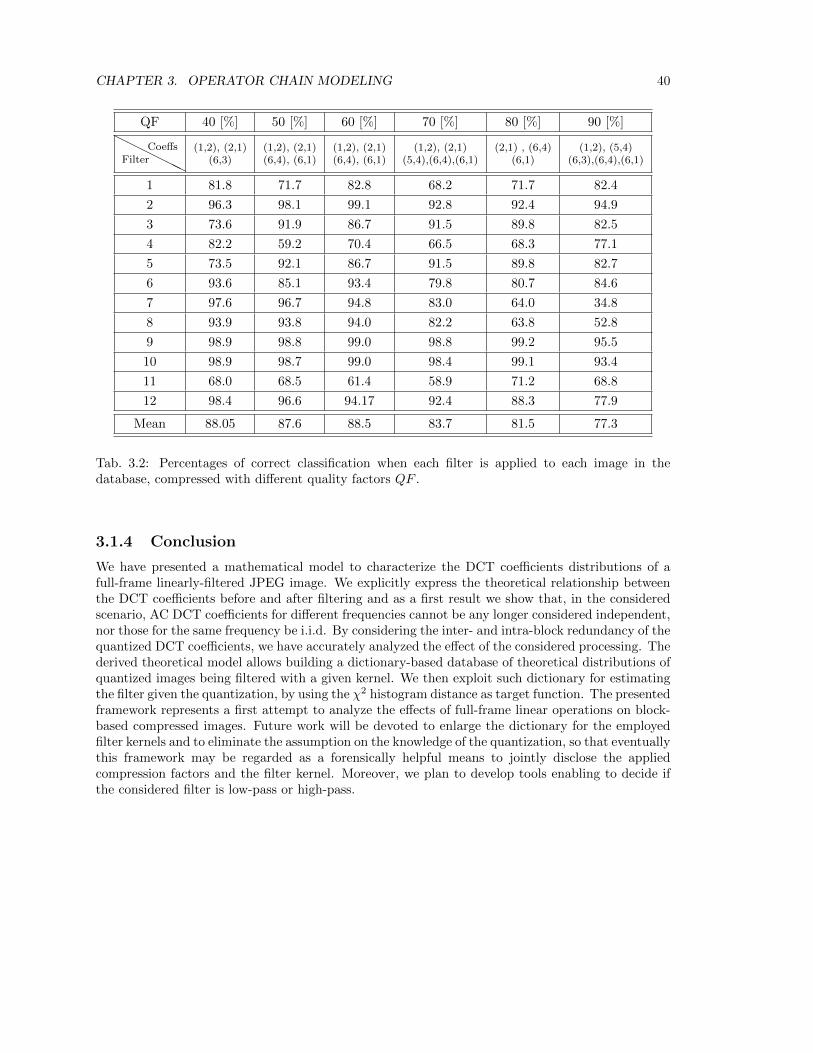
CHAPTER 3. OPERATOR CHAIN MODELING 40
QF 40 [%] 50 [%] 60 [%] 70 [%] 80 [%] 90 [%]HHHH
HHFilter
Coeffs (1,2), (2,1)(6,3)
(1,2), (2,1)(6,4), (6,1)
(1,2), (2,1)(6,4), (6,1)
(1,2), (2,1)(5,4),(6,4),(6,1)
(2,1) , (6,4)(6,1)
(1,2), (5,4)(6,3),(6,4),(6,1)
1 81.8 71.7 82.8 68.2 71.7 82.4
2 96.3 98.1 99.1 92.8 92.4 94.9
3 73.6 91.9 86.7 91.5 89.8 82.5
4 82.2 59.2 70.4 66.5 68.3 77.1
5 73.5 92.1 86.7 91.5 89.8 82.7
6 93.6 85.1 93.4 79.8 80.7 84.6
7 97.6 96.7 94.8 83.0 64.0 34.8
8 93.9 93.8 94.0 82.2 63.8 52.8
9 98.9 98.8 99.0 98.8 99.2 95.5
10 98.9 98.7 99.0 98.4 99.1 93.4
11 68.0 68.5 61.4 58.9 71.2 68.8
12 98.4 96.6 94.17 92.4 88.3 77.9
Mean 88.05 87.6 88.5 83.7 81.5 77.3
Tab. 3.2: Percentages of correct classification when each filter is applied to each image in thedatabase, compressed with different quality factors QF .
3.1.4 Conclusion
We have presented a mathematical model to characterize the DCT coefficients distributions of afull-frame linearly-filtered JPEG image. We explicitly express the theoretical relationship betweenthe DCT coefficients before and after filtering and as a first result we show that, in the consideredscenario, AC DCT coefficients for different frequencies cannot be any longer considered independent,nor those for the same frequency be i.i.d. By considering the inter- and intra-block redundancy of thequantized DCT coefficients, we have accurately analyzed the effect of the considered processing. Thederived theoretical model allows building a dictionary-based database of theoretical distributions ofquantized images being filtered with a given kernel. We then exploit such dictionary for estimatingthe filter given the quantization, by using the χ2 histogram distance as target function. The presentedframework represents a first attempt to analyze the effects of full-frame linear operations on block-based compressed images. Future work will be devoted to enlarge the dictionary for the employedfilter kernels and to eliminate the assumption on the knowledge of the quantization, so that eventuallythis framework may be regarded as a forensically helpful means to jointly disclose the appliedcompression factors and the filter kernel. Moreover, we plan to develop tools enabling to decide ifthe considered filter is low-pass or high-pass.

CHAPTER 3. OPERATOR CHAIN MODELING 41
QF 40 [%] 50 [%] 60 [%] 70 [%] 80 [%] 90 [%]
HHHH
HHFilter
Coeffs (1,2), (2,1)(2,2) (3,7)
(1,2),(2,2),(5,4)(6,4), (6,1)
(1,2), (2,2)(2,8)
(1,2) , (5,4)(6,4),(6,1)
(2,1) , (5,4)(6,4) , (6,1)
(6,3) , (6,4)(6,1)
1 90.3 82.9 91.8 78.8 80.0 93.4
2 98.8 98.6 98.95 99.1 98.2 86.1
3 95.2 88.9 94.8 94.9 90.1 91.0
4 80.4 69.5 85.8 73.8 77.6 87.0
5 65.2 88.9 94.8 95.1 90.3 91.0
6 95.4 90.6 96.4 84.75 85.8 91.9
9 99.6 98.9 99.9 97.9 99.1 92.4
10 99.4 98.5 99.7 96.6 97.9 88.5
Mean 94.3 89.7 95.3 90.1 89.8 90.2
Tab. 3.3: Percentages of correct classification when only low pass filters are considered.
QF 40 [%] 50 [%] 60 [%] 70 [%] 80 [%] 90 [%]
HHHHHH
FilterCoeffs (8,1),(6,1)
(1,8)(8,1),(6,1)
(2,8)(8,1), (6,2)
(2,8)(2,1) , (8,2), (7,1)(6,1),(6,2) , (2,8)
(8,1) , (7,2)(3,8)
(1,2),(8,1),(8,2)(7,2),(6,1),(3,8)
7 97.6 97.3 98.1 99.3 97.6 98.4
8 96.4 96.3 96.9 98.8 96.7 97.5
11 99.7 98.9 99.3 98.6 99.9 98.5
12 100 99.9 100 99.8 98.7 96.9
Mean 98.4 98.1 98.5 99.2 98.2 97.8
Tab. 3.4: Percentages of correct classification when only high pass filters are considered.
3.2 Interpolation estimation
The problem of resampling factor estimation for tampering detection is addressed following themaximum likelihood criterion in this section. By relying on the rounding operation applied af-ter resampling, an approximation of the likelihood function of the quantized resampled signal isobtained. From the underlying statistical model, the maximum likelihood estimate is derived forone-dimensional signals and a piecewise linear interpolation. The performance of the obtained esti-mator is evaluated, showing that it outperforms state-of-the-art methods.
3.2.1 Introduction
A well-known problem in this research area is the detection of resampling traces as a means tounveil the application of a geometric transformation and the estimation of the resampling factor forspecifying the parameters of the applied transformation.Seminal works addressing this topic [41, 42, 43], were focused on the detection of the particularcorrelation introduced between neighboring pixels by the resampling operation inherently presentwhen a spatial transformation (e.g., scaling or rotation) has been performed.Since the resampling operation can be modeled as a time-varying filtering that induces periodiccorrelations, links between this problem and the cyclostationarity theory have been established

CHAPTER 3. OPERATOR CHAIN MODELING 42
in [44] and [45], providing a theoretical framework for the estimation of the parameters of thetransformation. Within this framework, two different approaches have been proposed for finding theoptimum prefilter that might be applied to a resampled image for achieving the best performancein the estimation of the resampling factor [46, 47].At some point, all the mentioned approaches perform an analysis in the frequency domain for thedetection or estimation of this periodic behavior, by looking at spectral peaks corresponding tounderlying periodicities. Nevertheless, the frequency analysis presents some drawbacks: 1) a con-siderably large number of samples is needed to obtain reliable results; 2) the presence of periodicpatterns in the content of the image usually misleads the detector and the estimator; and 3) the win-dowing effect impairs the performance of the mentioned methods when slight spatial transformationsare employed (i.e., with a resampling factor near 1).With these shortcomings in mind, in this section we will address the estimation of the resamplingfactor following the Maximum Likelihood (ML) criterion. The approximation of the likelihoodfunction of the resampled signal will rely on the rounding operation applied after the resampling.Therefore, by correctly modeling the relationship between the distribution of the quantization noiseand the quantized resampled signal, an optimum estimator of the resampling factor will be provided.The proposed approach will only consider one-dimensional (1-D) signals, but the idea can easily beextended to the two-dimensional case, to be applied to images. The three discussed drawbacks ofthe previous methods will be sorted out with the proposed estimator.
3.2.2 Preliminaries and problem formulation
A digital image forgery can be done in many different ways, but it usually involves cropping someregion from a particular image and pasting it into a different one. The adjustment of this new contentto a specific scene is commonly carried out by applying geometrical transformations (e.g., rotationor scaling) that inherently need to perform a resampling operation. Since the tampering shouldnot introduce visible distortions, only slight transformations will be applied, thus requiring that theresampling estimator should achieve good performance for resampling factors near 1. This workjust studies the case where the resampling factor is larger than 1. Of course, the use of resamplingfactors smaller than 1 are commonly used; however, the analysis is formally quite different, so weleave the study of such case for a future work.The problem of resampling estimation is addressed for 1-D signals because the derivation of theMaximum Likelihood Estimate (MLE) of the resampling factor is more tractable and affordablethan considering directly the two-dimensional (2-D) case. However, we will see in Section 3.2.3that the obtained method following the ML criterion can be easily extended to the 2-D case. Thesame holds for the considered interpolation filter. The use of a piecewise linear interpolation schemeis a clear limitation of our work, which should be considered in this regard as a first attempt tointroduce MLE principles in the resampling estimation problem. We notice that the methodologyhere introduced can be extended to include more general filters.
3.2.2.1 Notation
A time-dependent 1-D signal will be represented as x(n). Random variables will be denoted bycapital letters (e.g., X) and their realizations by lowercase letters (e.g., x). Random vectors will berepresented with bold capital letters (e.g., X), their outcomes with lowercase letters (e.g., x) andeach ith component will be denoted as xi. The length of a vector x will be expressed as Lx ∈ N+ and,for convenience, the index i to identify each component of the vector will satisfy i ∈ {0, . . . , Lx− 1}.A vector of length N starting from the nth component, will be denoted by xn = (xn, . . . , xn+N−1)T .

CHAPTER 3. OPERATOR CHAIN MODELING 43
Floor and ceiling functions will be represented by b·c and d·e, respectively. To denote the set of allinteger numbers multiple of a given integer value n, we will use the notation nZ. For a compactnotation, we will use mod(a, b) to denote the modulo operation: a mod b.
3.2.2.2 Problem formulation
In the following, we will mathematically describe all the steps involved in the change of the samplingrate of a 1-D signal x(n), by a resampling factor denoted by ξ. This description will allow us toset out an approach based on the ML criterion in Section 3.2.3, for the estimation of the appliedresampling factor.Let us start by defining the resampling factor ξ as the ratio between the applied upsampling factorL and downsampling factor M , i.e., ξ , L
M with L ∈ N+ and M ∈ N+. To ensure a uniquerepresentation of ξ, we will consider that L and M are coprime, but note that this is not a limitation.As it was stated above, the possible range of values for the resampling factor will be ξ > 1. Forthis range of resampling factors, the general expression for a resampled signal y(n) is given by thefollowing relation with the original signal x(n):
y(n) =∑k
x(k)h
(nM
L− k),
where h(t) with t ∈ R represents the interpolation filter. As it was previously indicated, the inter-polation filter used during the resampling process will be assumed linear, with the following impulseresponse
h(t) =
{1− |t|, if |t| ≤ 1
0, otherwise.
Therefore, considering this interpolation filter, each component of the resampled vector can becomputed as the linear combination of at most two samples from the original signal,
y(n) =
x(⌊nML
⌋) (1−mod
(nML , 1
))+ x
(⌊nML
⌋+ 1)
mod(nML , 1
), if n /∈ LZ
x(nML
), if n ∈ LZ
.
Regarding the set of values that the original signal can take, we will consider that all the samplesx(n) have already been quantized by a uniform scalar quantizer with step size ∆, in order to fitinto a finite precision representation. Even though the interpolated values y(n) will be generallyrepresented with more bits, a requantization to the original precision is often done prior to saving theresulting signal. This quantized version of the resampled signal, denoted by z(n), will be expressedas
z(n) =
Q∆
(x(⌊nML
⌋) (1−mod
(nML , 1
))+ x
(⌊nML
⌋+ 1)
mod(nML , 1
)), if n /∈ LZ
x(nML
), if n ∈ LZ
, (3.10)
where Q∆(·) represents a uniform scalar quantization with step size ∆ (i.e., the same one used forthe original signal).From the second condition in (3.10), it is evident that some of the original samples are “visible” inthe quantized resampled version. On the other hand, the remaining values of the resampled signalare the combination of “visible” and “non-visible” samples from the original signal that are laterquantized. This fact will help to define the likelihood function of the quantized resampled signal.

CHAPTER 3. OPERATOR CHAIN MODELING 44
3.2.3 ML approach to resampling estimation
For the definition of the MLE of ξ, the original signal will be represented by the vector x with Lxsamples and the corresponding quantized resampled signal by the vector z with Lz samples. Forconvenience, we will assume that the length of the original signal is Lx = N + 1 with N a multipleof M , and so, the corresponding length of the resampled signal will be Lz = ξN + 1. We will findit convenient to model vectors x and z as outcomes of random vectors X and Z, respectively.Based on the above analysis, the estimation of the resampling factor ξ following the ML criterionrelies on finding the value of ξ that makes the observed values of the quantized resampled vector zmost likely. Nevertheless, given a vector of observations, their components zi could be misalignedwith the periodic structure of the resampled signal in (3.10). Hence, a parameter φ must be consid-ered to shift the components of the vector, in order to align the periodic structure of zi with z(n).The possible values of φ lie in the range 0 ≤ φ ≤ L− 1. Therefore, the MLE of ξ becomes
ξ = arg maxξ>1
max0≤φ≤L−1
fZ|Ξ,Φ(z|ξ, φ).
Note that we are not considering a set of possible parameters for the interpolation filter becausein the case of a piecewise linear interpolation, once we fix the resampling factor, then the filteris automatically determined (cf. Eq. (3.10)). On the other hand, given that the shift φ is not adetermining factor for the derivation of the target function, for the sake of simplicity, we will assumethat the vector of observations is correctly aligned and, thus, the MLE can be written as
ξ = arg maxξ>1
fZ|Ξ(z|ξ).
For the calculation of that joint probability density function (pdf) we will exploit the fact that somesamples of the interpolated signal exactly match the original (cf. Eq. (3.10)), and also the linearrelation established between the remaining samples.
3.2.3.1 Derivation of fZ|Ξ(z|ξ)Along the derivation of the joint pdf fZ|Ξ(z|ξ), for the sake of notational simplicity, we will referto this one as fZ(z), considering implicitly that we are assuming a particular resampling factor ξ.From the dependence between the quantized resampled signal and the original one, the joint pdfcan be written in a general way as
fZ(z) =
∫RN+1
fZ|X(z|x)fX(x)dx.
We assume that no a priori knowledge on the distribution of the input signal is available. This isequivalent to considering that fX(x) is uniform and, consequently, the joint pdf can be approximatedby the following relation
fZ(z) ≈∫RN+1
fZ|X(z|x)dx.
Equation (3.10), indicates that every L samples of the observed vector z, we have a visible samplefrom the original signal. This implies that the random variable Zi, given Xk, is deterministicwhenever i ∈ LZ and k ∈MZ. For this reason, the previous joint pdf can be obtained by processing(Lz − 1)/L = N/M distinct and disjoint blocks, i.e.,
fZ(z) ≈N/M−1∏j=0
∫RM
fZLj |XMj(zLj |xMj)dxMj , (3.11)

CHAPTER 3. OPERATOR CHAIN MODELING 45
−0.2 0 0.2 0.4 0.6 0.8 1 1.20
0.5
1
1.5
2
2.5
3
3.5
4
4.5
5
xk
zi
xk+1
(a) zi between xk and xk+1
0 2 4 6 8−1
0
1
2
3
4
5
6
7
xk+1
zi
(b) Feasible interval and pdf
−0.2 0 0.2 0.4 0.6 0.8 1 1.20
1
2
3
4
5
6
7
zi+1
xk+1
xk
zi
(c) zi, zi+1 between xk and xk+1
0 2 4 6 8−1
0
1
2
3
4
5
6
7
Δ
Δ
xk+1
zi
zi+1
(d) Feasible interval and pdf
Figure 3.5: Illustrative example, showing the last two possible cases for zi. Pdfs obtained are showngraphically. Note that ∆ = 1.
where ZLj and XMj (and also their corresponding outcomes) are vectors of size L and M , respec-tively.The calculation of the contribution of each block of L samples from the vector of observations zLjin (3.11), will depend on its relation with the corresponding M samples of the vector of the originalsignal, i.e., xMj . This relation is determined by the assumed resampling factor ξ.Therefore, considering an arbitrary sample zi that will be linearly related with at most two originalsamples xk and xk+1, with k ,
⌊iML⌋
(cf. Eq. (3.10)), three cases are possible:
• zi is a visible sample, thus deterministic. Consequently
fZi|Xk(zi|xk) = δ(zi − xk),
where δ(·) represents the Dirac delta.
• zi is the only sample between two original ones as it is shown in Fig. 3.5(a). In this case, if thevariance of the original signal is large enough with respect to the variance of the quantizationnoise, then the quantization error can be considered uniform (we will call this the “fine-quantization assumption”), and the obtained pdf is
fZi|Xk,Xk+1(zi|xk, xk+1) = Π
(aixk + bixk+1 − zi
∆
),
where Π(t) denotes a rectangular pulse that is 1 if t ∈[− 1
2 ,12
]and 0 otherwise. In this case,
for the sake of clarity, we have used ai , (1 − mod(iML , 1)) and bi , mod(iML , 1), obtainedfrom (3.10). A graphical representation, depicted in Fig. 3.5(b), shows how the rectangularpdf is derived from zi.

CHAPTER 3. OPERATOR CHAIN MODELING 46
• zi is one of several resampled values between two original samples, as it is shown in Fig. 3.5(c).As before, the following pdf is valid if the fine-quantization assumption holds, hence
fZi|Xk,Xk+1(zi|xk, xk+1)
=∏m
Π
(amxk + bmxk+1 − zm
∆
),
where m will increase from i to the number of resampled values located between the twooriginal samples. Fig. 3.5(d) shows the resulting pdf for the considered example.
Each time we obtain the pdf for a particular zi (or a group of them), the corresponding integral in(3.11) must be evaluated with respect to the corresponding original sample xk. Intuitively, we canobserve that the calculation of (3.11) will finally be the convolution of several rectangular functions,leading to a feasible and easy implementation. Note that those uniform distributions are obtainedonly if the fine-quantization assumption holds. Given the importance of this assumption, its effecton the performance of the MLE will be analyzed in Section 3.2.4.
3.2.3.2 Method description
For a better understanding on how the obtained MLE can be easily implemented, we will exemplifythe calculation of the target function fZ|Ξ(z|ξ) when a particular resampling factor ξt is tested. Inthis illustrative example we will consider a vector of observations z (already aligned), correspondingto a signal that has been resampled by a factor ξ = 5
3 . In Fig. 3.6(a), an example of this vector ofobservations is shown, along with the corresponding vector of original samples x. In the mentionedfigure, solid lines are used for representing the resampled values (consequently, also the originalsamples that are visible), while dashed lines are used for representing the non-visible samples of theoriginal signal.Since the calculation of the target function fZ|Ξ(z|ξ) can be split by processing blocks of L samples ofthe observed vector, in this example, we will show how to process a single block. For the calculationof the remaining blocks, the same process should be repeated. Assuming that the resampling factorunder test is ξt = 5
3 , these are the followed steps:
1. The first sample z0 is a visible one, then we know that z0 = x0 and, thus, fZ0|X0,Ξ(z0|x0, ξt) =δ(z0 − x0).
2. The second sample z1 is located between two original samples, i.e., the visible x0 and thenon-visible x1. Hence, we have fZ1|X0,X1,Ξ(z0|x0, x1, ξt) = Π
(a1x0+b1x1−z1
∆
).
Fig. 3.6(b) shows with a red line the linear relation between the interpolated value and theoriginal ones y1 = a1x0 + b1x1, with the value of x0 fixed, i.e., from the previous step x0 = z0.From the value of z1 we obtain the feasible interval of x1 (represented with dashed blacklines). Finally, the resulting pdf after the convolution of the rectangular function with thedelta obtained in Step 1 is plotted in green.
3. The third and fourth samples, z2 and z3, are located between the two original samples x1 andx2. In this case, we have seen that fZ2|X1,X2,Ξ(z2|x1, x2, ξt) = Π
(a2x1+b2x2−z2
∆
)Π(a2x1+b2x2−z3
∆
).
Fig. 3.6(c) shows in this case the corresponding two linear relations for y2 = a2x1 + b2x2 andy3 = a3x1 + b3x2. Be aware that in this case x1 can take any value in the range obtained inStep 2, and that is the reason why the dashed red lines are plotted. From the product of thetwo rectangular pdfs, we obtain the feasible interval for x2 (whose pdf is represented in cyan).

CHAPTER 3. OPERATOR CHAIN MODELING 47
0 0.5 1 1.5 2 2.5 30
1
2
3
4
5
6
7
Original signalResampled signal
x0
z0
z1
x1
z2
z3
x2
z4
z5
x3
(a) Original and resampled signals
0 1 2 3 4 5 6
0
1
2
3
4
5
6
7
Δ
z1
x1
(b) Resulting pdf in Step 2
0 2 4 6 8 10 12
0
1
2
3
4
5
6
7
Δ
Δ
x2
z2 z
3
(c) Feasible interval for x2
0 1 2 3 4 5 6 7
0
0.5
1
1.5
2
2.5
3
x2
(d) Resulting pdf in Step 3
−2 0 2 4 6
0
0.5
1
1.5
2
2.5
3
x3
(e) Resulting pdf in Step 4
Figure 3.6: Graphical representation of the method description. Note that ∆ = 1.
At this point, it is important to note that when the resampling factor under test does notmatch the true one, the previous product of rectangular pdfs could lead to an empty feasibleset for x2. If this happened, then we would automatically infer the infeasibility of the testedresampling factor, so the estimation algorithm would move to the next resampling factor inthe candidate set.
If the factor cannot be discarded, then we must compute the convolution of the uniform pdfhere obtained with the one resulting from Step 2. The result is plotted in green in Fig. 3.6(d).
4. The fifth sample z4 is processed in the same way as in Step 2, but considering that nowthe linear relation y4 = a4x2 + b4x3 must be evaluated with the set of possible values of x2.Proceeding this way, we obtain the feasible interval for x3 and the corresponding pdf. Bothare shown in Fig. 3.6(e).
5. At this point, we have finished processing the L samples in the block and we have the resultingpdf as a function of x3. Since the next sample is visible, i.e., z5 = x3, to determine thecontribution of these L samples to the target function fZ|Ξ(z|ξt), we evaluate the resultingpdf taking into account the actual value of z5.

CHAPTER 3. OPERATOR CHAIN MODELING 48
As before, if the value of z5 falls outside the possible range of x3, then the resampling factorunder test is discarded.
Following this procedure, the maximization of the target function fZ|Ξ(z|ξ) is performed over the
set of candidate resampling factors ξ > 1 that have not been discarded, achieving the MLE ξ. Afterthis qualitative explanation, it is clear that the 2-D extension of this method is straightforward.
3.2.4 Experimental results
The experimental validation of the obtained MLE is divided in two parts. In the first one, theperformance of the estimator is evaluated by using synthetic signals and its behavior in terms of thefine-quantization assumption is analyzed. In the second part, natural 1-D signals from the audiodatabase in [48] (which contains different music styles) are used to test the estimator in a morerealistic scenario. To confirm that the described method is able to sort out the drawbacks pointedout in the Introduction, comparative results with a 1-D version of the resampling detector proposedby Popescu and Farid in [41] are also provided.
3.2.4.1 Performance analysis with synthetic signals
In this case, we consider as synthetic signal a first-order autoregressive (AR) process, parameterizedby a single correlation coefficient ρ. The AR(1) model is commonly used for characterizing thecorrelation between samples of natural signals, where the value of ρ adjusts the model. Typically,close to 1 values are considered for modeling natural signals, as it is done with images [49]; hence,ρ = 0.95 will be used in the following simulations. The AR(1) process has the following form
u(n) = w(n) + ρu(n− 1),
where w(n) is a Gaussian process with zero mean and variance σ2W . Note that in this case, the
process w(n) is actually the innovation from one sample to another of the AR(1) process, so resultswill be drawn as a function of σ2
W to evaluate the validity of the fine-quantization assumption.To reproduce the conditions of the considered model, the original signal x(n) is obtained by quantiz-ing the generated AR(1) process, i.e., x(n) = Q∆ (u(n)) with ∆ = 1. Regarding the set of consideredresampling factors, for the sake of simplicity, we use a finite discrete set, obtained by sampling theinterval (1, 5] with step size 0.05 (from 1.05 to 2) and 0.5 (from 2 to 5). Be aware that we use thesame set for the true resampling factor ξ and the values tested by the ML estimator, ξt. We considerthat the estimation of the resampling factor is correct if ξ = ξ, i.e., if the estimated value is indeedthe one used for resampling the original signal, up to the precision used when griding ξ and ξt. Forall the experiments, the length of the vector of observations is Lz = 400.Fig. 3.7 shows the percentage of correct estimation for some of the resampling factors in the set asa function of σ2
W . From this plot, we can observe that the performance of the estimator stronglydepends on the mentioned variance of innovation, as well as on the true resampling factor used.For instance, by resampling the AR process with ξ = 5, a very small value for the variance ofinnovation (σ2
W = 0.5), is required to correctly estimate the resampling factor for all the experiments;nevertheless, for ξ = 2, almost a value of σ2
W = 50 will be necessary for getting the same estimationperformance. In general, and in accordance with the assumptions backing the analysis introducedin the previous section, the higher σ2
W , the better the estimation will be.Although ML-based estimators are frequently thought to be computationally demanding, if the fine-quantization assumption holds, then the estimation proposed in the previous section is very cheapand only a few samples are required for correctly estimating the actual resampling factor. Remember

CHAPTER 3. OPERATOR CHAIN MODELING 49
100
101
102
0
10
20
30
40
50
60
70
80
90
100
σW2
Cor
rect
res
ampl
ing
fact
or e
stim
atio
n [%
]
ξ = 1.05ξ = 1.10ξ = 1.20ξ = 1.30ξ = 1.40ξ = 1.50ξ = 1.60ξ = 1.70ξ = 1.80ξ = 1.90ξ = 2.00ξ = 2.50ξ = 3.50ξ = 5.00
Figure 3.7: Correct resampling factor estimation percentage for different resampling factors as afunction of σ2
W . ρ = 0.95, and 500 Monte Carlo realizations are considered.
1 1.1 1.2 1.3 1.4 1.5 1.6 1.7 1.8 1.9 20
50
100
150
200
250
300
350
400
450
Num
ber
of p
roce
ssed
sam
ples
(ov
er 4
00)
ξt (tested resampling factors)
σ
W2 = 0.5
σW2 = 10
σW2 = 40
σW2 = 80
Figure 3.8: Number of discarded samples for different values of σ2W , as a function of ξt. The true
resampling factor is ξ = 32 . 500 Monte Carlo realizations were performed.
that when a resampling factor under test does not match the true one, then it can be discardedwhen an empty set is obtained for a non-visible sample or when a visible sample falls outside theobtained interval (cf. Steps 3 and 5 in Section 3.2.3.2).This is illustrated at Fig. 3.8, where the number of samples required for discarding the candidateresampling factor is shown for different values of σ2
W , when ξ = 32 . As it can be checked in that
figure, whenever the ξt = ξ, the tested resampling factor will not be discarded, even when the fullvector of observations is considered, as it should be expected. It is also important to point out thatthe larger the value of σ2
W , i.e., the more accurate the fine-quantization assumption is, the smallernumber of samples is required for discarding a wrong ξt.
3.2.4.2 Performance analysis with real audio signals
For the evaluation of the estimator in a real scenario, we consider the “Music Genres” audio database[48], composed of 1000 uncompressed audio files with 10 different music styles (for instance some

CHAPTER 3. OPERATOR CHAIN MODELING 50
1.05 1.1 1.2 1.3 1.4 1.5 1.6 1.7 1.8 1.9 20
10
20
30
40
50
60
70
80
90
100
ξ (true resampling factor)
Cor
rect
res
ampl
ing
fact
or e
stim
atio
n [%
]
Lz=64
Lz=128
Lz=256
Lz=512
Figure 3.9: Comparison of the correct estimation percentage of the proposed MLE versus the methodproposed in [41]. Solid lines represent the obtained results with the MLE, while dashed lines areused for the method [41].
of them are blues, country, jazz, pop or rock). The performance of the proposed estimator will bechecked by fixing the number of available samples, and looking for inconsistencies in the resampledsignal with respect to the tested resampling factor. For comparison, the same tests will be performedwith a state-of-the-art resampling detector, i.e., the one proposed by Popescu and Farid in [41].1
The set of resampling factors that we will consider in this case will be in the interval (1, 2] (sampledwith a step size of 0.05). Since we are interested in comparing the performance with differentsizes for the vector of observations, we perform the experiments with the following set of valuesLz ∈ {64, 128, 256, 512}.The results obtained with both methods are shown in Fig. 3.9. As we can observe, the methodproposed by Popescu and Farid is highly dependent on the number of available samples, whereasour proposed MLE is essentially independent of this parameter. In the same way, the performanceachieved by their method is poor when the applied resampling factor is close to 1, which is neitheran issue for our estimator. These two limitations of Popescu and Farid’s method come from thefrequency analysis performed (once the pmap has been computed) for the detection of the resamplingfactor, as we pointed out in the Introduction. From these results, it is clear that the MLE methodbecomes very useful for estimating the resampling factor when a small number of samples areavailable, thus leading to a very practical forensic tool.Although the performance of the MLE is very good, if we consider a noisy vector of observationsthen the method of Popescu and Farid is expected to be more robust than the proposed MLE. Thereason is that in their model for the EM algorithm, they assume Gaussian noise, and in our case,we are only assuming the presence of uniformly distributed noise, due to the quantization. We note,however, that it is possible to extend our model to the case of Gaussian noise. Such extension is leftfor future research.
1The neighborhood of the predictor is set to N = 3, yielding a window of length 7.

CHAPTER 3. OPERATOR CHAIN MODELING 51
3.2.5 Conclusions
The problem of resampling factor estimation following the ML criterion has been investigated in thissection for the 1-D case. The derived MLE from this analysis has been tested with audio signalsshowing very good performance. The most distinctive characteristic of the proposed approach isthat only a few number of samples of the resampled signal is needed to correctly estimate the usedresampling factor.Since the scenario where the proposed resampling factor estimator can be employed is quite limited,future work will focus on improving this aspect. As a first step, the 2-D extension of the obtainedmethod will be explicitly derived. Introduction of new parameters in the model such as general inter-polation filters, noisy observations or resampling factors smaller than one will be studied. Possiblelinks between this work and set membership algorithms will also be considered.
3.3 Transform coder identification based on quantization foot-prints and lattice theory
Transform coding is routinely used for lossy compression of discrete sources with memory. Theinput signal is divided into N -dimensional vectors, which are transformed by means of a linearmapping. Then, transform coefficients are quantized and entropy coded. In this section we considerthe problem of identifying the transform matrix as well as the quantization step sizes. We study thechallenging case in which the only available information is a set of P transform decoded vectors. Weformulate the problem in terms of finding the lattice with the largest determinant that contains allobserved vectors. We propose an algorithm that is able to find the optimal solution and we formallystudy its convergence properties. Our analysis shows that it is possible to identify successfully boththe transform and the quantization step sizes when P ≥ N + δ where δ is a small integer, and theprobability of failure decreases exponentially to zero as P −N increases.
3.3.1 Introduction
Due to its centrality to any type of multimedia data, transform coding theory is now extensivelyused in a new range of applications that rely on the possibility of reverse-engineering complex chainsof operators starting from the available output signals. Indeed, the lifespan of a multimedia signal isvirtually unbounded. This is due to the ability of creating copies and the availability of inexpensivestorage options. However, signals seldom remain identical to their original version. As they passthrough processing chains, some operators, including transform coding, are bound to leave subtlecharacteristic footprints on the signals, which can be identified in order to uncover their processinghistory. This insight might be extremely useful in a wide range of scenarios in the field of multimediasignal processing at large including, e.g.,: i) forensics, in order to address tasks such as source deviceidentification [50] or tampering detection [51][35]; ii) quality assessment, to enable no-referencemethods that rely solely on the received signals [52][53]; iii) digital restoration, which requires priorknowledge about the operations that affected a digital signal [54].In this context, several works have exploited the footprints left by transform coding. In [55], a methodwas proposed to infer the implementation-dependent quantization matrix template used in a JPEG-compressed image. Double JPEG compression introduces characteristic peaks in the histogram ofDCT coefficients, which can be detected and used, e.g, for tampering localization [56][35]. Morerecently, similar techniques were applied to video signals for the cases of MPEG-2 [57][58], MPEG-4 [59][60] and H.264/AVC [61].

CHAPTER 3. OPERATOR CHAIN MODELING 52
All the aforementioned works require prior knowledge of the type of standard being considered. Thisimplies that the specific transform in use is assumed to be known, whereas the quantization stepsizes need to be estimated. In practice, it might be useful to be able to infer which transform wasused in order to understand, for example, whether an image was compressed using the DCT-basedJPEG or the wavelet-based JPEG 2000 and, in the latter case, which wavelet transform was used.Similarly, it would be good to be able to infer if a video sequence was compressed using MPEG-2,MPEG-4 or H.264/AVC. Some efforts in this direction can be found in [62].Most of the above methods focus only on a specific type of multimedia signal (e.g., only images oronly videos) and are to some extent heuristic. It is therefore natural to try and develop a universaltheory of transform coder identification that is independent of the specific application at hand. Tothis end, here we consider a general model of transform coding that can be tailored to describe alarge variety of practical implementations that are found in lossy coding systems, including thoseadopted in multimedia communication. Specifically, a 1-dimensional input signal is encoded bypartitioning it into non-overlapping N -dimensional vectors, which are then transformed by meansof a linear mapping. Then, transform coefficients are quantized and entropy coded. At the decoder,quantization symbols are entropy decoded and mapped to reconstruction levels. Then, the inversetransform is applied to obtain an approximation of the signal in its original domain.Given the output produced by a specific transform coding chain, we investigate the problem of iden-tifying its parameters. To this end, we assume both the size and the alignment of the transform tobe known, as they can be estimated with methods available in the literature [58][55]. We propose analgorithm that receives as input a set of P transform decoded vectors embedded in a N -dimensionalvector space and produces as output an estimation of the transform adopted, as well as the quan-tization step sizes, whenever these can be unambiguously determined. We leverage the intrinsicdiscrete nature of the problem, by observing the fact that these vectors are bound to belong to aN -dimensional lattice. Hence, the problem is formulated in terms of finding a lattice that containsall observed vectors. We propose an algorithm that is able to solve the problem and we formallystudy its convergence properties. Our analysis shows that it is possible to successfully identify boththe transform and the quantization step sizes with high probability when P > N . In the experimentswe found that an excess of approximately 6-7 observed vectors beyond the dimension N of the spaceis generally sufficient to ensure successful convergence. In addition, the complexity of the algorithmis shown to grow linearly with N .It is important to mention that the method used to solve the problem addressed in this workis related to Euclid’s algorithm, which is used to find the greatest common divisor (GCD) in aset of integers. Indeed, when N = 1 and P = 2, the proposed method coincides with Euclid’salgorithm. However, in this case the problem reduces to estimating the quantization step size, asthe transform is trivially defined. Note that, lattice theory has been widely used for source andchannel coding (e.g., [63, 64, 65]). However, to the best of the authors’ knowledge, this theory hasnot been employed to address the problem of identifying a linear mapping using the footprint left byquantization. Only [25] uses similar principles but their goal is to investigate the color compressionhistory, i.e., the colorspace used in JPEG compression. Therefore, the solution proposed is tailoredto work in a 3-dimensional vector space, thus avoiding the challenges that arise in higher dimensionalspaces.Also, it is important not to confuse the problem addressed here with the classical problem of latticereduction [65]. In the latter case, given a basis for a lattice, one seeks an equivalent basis matrixwith favorable properties. Usually, such a basis consists of vectors that are short and with improvedorthogonality. There are several definitions of lattice reduction with corresponding reduction criteria,each meeting a different tradeoff between quality of the reduced basis and the computational effortrequired for finding it. The most popular one is the Lenstra-Lenstra-Lovasz (LLL) reduction [66],

CHAPTER 3. OPERATOR CHAIN MODELING 53
which can be interpreted as an extension of the Gauss reduction to lattices of rank greater than 2.The rest of this section is organized as follows. Section 3.3.2 introduces the necessary notationand formulates the transform identification problem and Section 3.3.3 provides the background onlattice theory. The proposed method is described in Section 3.3.4. Then, a theoretical analysis of theconvergence properties is presented in Section 3.3.5. The performance of the transform identificationalgorithm is evaluated empirically in Section 3.3.6. Finally, Section 3.3.7 indicates the open issuesand stimulating further investigations.
3.3.2 Problem statement
The symbols x, x and X denote, respectively, a scalar, a column vector and a matrix. A M × Nmatrix X can be written either in terms of its columns or rows. Specifically,
X =[
x1 x2 . . . xN]
=
xT1xT2· · ·xTM
. (3.12)
Let x denote a N -dimensional vector and W a transform matrix, whose rows represent the transformbasis functions.Transform coding is performed by applying scalar quantization to the transform coefficients y = Wx.Let Qi(·) denote the quantizer associated to the i-th transform coefficient. We assume that Qi(·) isa scalar uniform quantizer with step size ∆i, i = 1, . . . , N . Therefore, the reconstructed quantizedcoefficients can be written as y = [y1, y2, . . . , yN ]T , with
yi = Qi(yi) = ∆i · round
[yi∆i
], i = 1, . . . , N. (3.13)
The reconstructed block in the original domain is given by x = W−1y.Let {x1, . . . , xP } denote a set of P observed N -dimensional vectors, which are the output of atransform coder. Due to quantization, the unobserved vectors representing quantized transformcoefficients {y1, . . . , yP } are constrained to belong to a lattice Ly described by the following basis:
By =
∆1 0 . . . 00 ∆2 . . . 0...
.... . .
...0 0 . . . ∆N
(3.14)
Therefore, the observed vectors {x1, . . . , xP } belong to a lattice Lx described by the basis:
Bx = [bx,1, . . . ,bx,N ] = W−1By, (3.15)
with bx,i = ∆iwi, i = 1, . . . , N , W−1 = [w1, . . . , wN ].In this work we study the problem of determining Bx from a finite set of P ≥ N distinct vectors{x1, . . . , xP }. That is, we seek to determine the parameters of a transform coder based on thefootprints left on its output. We propose an algorithm to solve this problem and we study itsconvergence properties. In addition, we show that the probability of correctly determining Bx
(or, equivalently, another basis for the lattice Lx) is monotonically increasing in the number ofobservations P , and rapidly approaching one when P > N .

CHAPTER 3. OPERATOR CHAIN MODELING 54
b1
b2
P(B)
(a)
b1
z
← B · �B−1z�
Pz(B)b1
b2
(b)
b1
b2P(B)
(c)
P(B) →
P(B)
b1
b2
b2
b1
(d)
Figure 3.10: Examples of lattices. (a) The fundamental parallelotope of a lattice defined by a basisB. (b) Parallelotope enclosing an arbitrary vector z. (c) Another (equivalent) basis for the latticein (a). (d) An example of a sub-lattice of the lattice L(B).
Note that when determining Bx, the proposed method does not make any assumption on the struc-ture of the transform matrix W. In the general case, given Bx, it is not possible to uniquelydetermine W and the quantization step sizes ∆i, i = 1, . . . , N . Indeed, the length of each basisvector bx,i can be factored out as ‖bx,i‖2 = ∆i‖wi‖2. However, in the important case in which Wrepresents an orthonormal transform, the quantization step sizes ∆i, i = 1, . . . , N , and the transformmatrix W can be immediately obtained from Bx. Indeed, W−1 = WT , wi = wi, i = 1, . . . , N ,with ‖wi‖2 = 1. Therefore:
∆i = ‖bx,i‖2, i = 1, . . . , N, (3.16)
wi = bx,i/‖bx,i‖2 i = 1, . . . , N. (3.17)
3.3.3 Background on lattice theory
In this section we provide the necessary background on lattice theory. Further details can be found,e.g., in [67][68][65]. Let L denote a lattice of rank K embedded in RN . Let B = [b1,b2, . . . ,bK ]denote a basis for the lattice L. That is,
L = {x|a1b1 + a2b2 + . . .+ aKbK , ai ∈ Z}. (3.18)

CHAPTER 3. OPERATOR CHAIN MODELING 55
In order to make the mapping between a basis and the corresponding lattice explicit, the latter canbe expressed as L(B).Any lattice basis also describes a fundamental parallelotope according to
P(B) =
{x|x =
K∑i=1
θibi, 0 ≤ θi < 1
}. (3.19)
When K = 2, 3, P(B) is, respectively, a parallelogram or a parallelepiped. As an example, Fig-ure 3.10(a) shows the fundamental parallelotope corresponding to a lattice basis B when K = 2.Given a point z ∈ RK , let Pz(B) denote the parallelotope enclosing z. Pz(B) is obtained bytranslating P(B) so that its origin coincides with one of the lattice points. More specifically,
Pz(B) =
{x|x = B ·
⌊B−1z
⌋+
K∑i=1
θibi, 0 ≤ θi < 1
}. (3.20)
Figure 3.10(b) illustrates Pz(B) for an arbitrary vector z.Different bases for the same lattice lead to different fundamental parallelotopes. For example,Figure 3.10(a) and Figure 3.10(c) depict two different bases for the same lattice, together with thecorresponding fundamental parallelotopes. However, the volume of P(B) is the same for all basesof a given lattice. This volume equals the so-called lattice determinant, which is a lattice invariantdefined as
|L| =√
det(BTB). (3.21)
If the lattice is full rank, i.e., K = N , the lattice determinant equals the determinant of the matrixB, |L| = |det(B)|.Let L denote a sub-lattice of L. That is, for any vector x ∈ L, then x ∈ L. A basis B for L can beexpressed in terms of B as
B = BU, (3.22)
where U is such that uij ∈ Z. Moreover, let det(U) = ±m, then
|L||L| = |det(U)| = m (3.23)
and we say that L is a sub-lattice of L of index m. For example, Figure 3.10(d) shows two latticesL and L, such that L ⊂ L. In this case, the matrix U is equal to
U =
[−4 −53 −1
], (3.24)
and L is a sub-lattice of index m = 19.
3.3.4 An algorithm for transform identification
In this section we propose an algorithm that is able to determine the parameters of a transformcoder from its output, i.e., a set of observed vectors {x1, . . . , xP }. This is accomplished by findinga suitable lattice L∗ such that {x1, . . . , xP } ⊂ L∗. In Section 3.3.5.3 we will show that, withprobability approaching one, L∗ ≡ Lx, provided that P −N > 0.The problem of determining a basis for the lattice Lx is complicated by the fact that we typicallyobserve a finite (and possibly small) number of vectors P embedded in a possibly large dimensional

CHAPTER 3. OPERATOR CHAIN MODELING 56
space. More precisely, {x1, . . . , xP } belong to a bounded lattice, in virtue of the fact that eachtransform coefficient yi is quantized with a finite number of bits Ri, to one of 2Ri reconstructionlevels. Let R denote the average number of bits allocated to transform coefficients. The number ofpotential lattice points is equal to
N∏i=1
2Ri = 2∑Ni=1 Ri = 2NR, (3.25)
and only P of them are covered by observed vectors. Thus, we note that, given R, the numberof lattice points increases exponentially with the dimension N and that in most cases of practicalrelevance P � 2NR.Another issue arises from the fact that, for a set of vectors {x1, . . . , xP }, there are infinitely manylattices that include all of them. Indeed, any lattice L such that Lx ⊂ L is compatible with theobserved set of vectors. Note that any basis of the form B = BxU
−1, with det(U) = ±m, with man integer greater than one defines a compatible lattice L. A simple example is obtained settingU = aI, a ∈ N, a > 1.In order to resolve this ambiguity, we seek the lattice L∗ that maximizes the lattice determinant |L|,within this infinite set of compatible lattices. That is,
maximizeL(B)
|L(B)|subject to {x1, . . . , xP } ⊂ L(B).
(3.26)
For example, for the set of observed points {x1, x2, x3} depicted in Figure 3.11(a), Figure 3.11(g)illustrates a basis for the lattice that is the optimal solution of (3.26). In contrast, the lattice inFigure 3.11(h) is a feasible solution of (3.26), but it is not optimal, since it is characterized by alower value of the lattice determinant.The proposed method used to solve the problem above is detailed in Algorithm 1. The methodconstructs an initial basis for an N -dimensional lattice (line 1). This is accomplished by consideringthe vectors in O until N linearly independent vectors are found. These vectors are used as columnsof the starting estimate B(0) and to populate the initial set of visited vectors S. We denote with Uthe set of vectors in O that have not been visited yet. Then, the solution of (3.26) is constructediteratively, by considering the remaining vectors in U one by one. At each iteration, the functionrecurseTI returns a basis for a lattice that solves (3.26), in which the constraint is imposed only onthe subset of visited vectors S, that is, S ⊂ L(B). As such, the algorithm starts finding the solutionof an under-constrained problem and additional constraints are added as more vectors are visited.Figure 3.11 shows an illustrative example when N = 2 and three vectors {x1, x2, x3} are observed(Figure 3.11(b)). The initial basis (line 1) is constructed using x1 and x2, since they are linearly inde-pendent (Figure 3.11(b)). Then, the point x3 is selected (line 6 and Figure 3.11(c)) and the functionrecurseTI (line 9) returns a basis that solves (3.26), i.e., a basis with the largest lattice determinantthat includes all observed vectors. Figure 3.11(f) illustrates such a basis, and Figure 3.11(g) showsan equivalent basis obtained after lattice reduction.The core of the method is the recursive function recurseTI. When describing this function, wekeep a clear distinction between algorithm template and algorithm instance, as it is customaryin computer science. We start describing the template in Algorithm 2, which does not specifythe function entirely. Then, a concrete instance of the template is detailed in Algorithm 3. Therationale of maintaining this distinction is motivated by the fact that the correctness of the method isa property that descends from the template alone, as further discussed in Section 3.3.5.1. Conversely,the rate of convergence depends on the specific algorithm instance, as explained in Section 3.3.5.2.

CHAPTER 3. OPERATOR CHAIN MODELING 57
x3
x1
x2
(a)
x1
x2
(b)
x3
x1
x2
(c)
x3
x1
x2
(d)
x3
x1
x2
(e)
x3
x1
x2
(f)
x3
x1
x2
(g)
x3
x1
x2
(h)
Figure 3.11: An example of transform identification. A set of three observed vectors is given in (a).Then, (b)-(h) show, step-by-step, how the solution to problem (3.26) is sought by Algorithm 1.
3.3.4.1 An algorithm template for recurseTI
The function recurseTI receives as input a set of visited vectors S and the current estimate of abasis B for the lattice L(B). If S ⊂ L, i.e., all the vectors in S belong to the lattice defined by B,the recursion is terminated (line 1 in Algorithm 2). Otherwise, one of the vectors x that does notbelong to L is selected (line 4) and the parallelotope which encloses it is identified (line 5). Then, avector d is computed as the difference between x and one of the vertices of the parallelotope (line 6).The intuition here is to capture a short vector that cannot be represented by the current lattice, andto modify the current basis in such a way that (upon convergence) it can be represented. Hence,the updated basis is constructed by replacing one of the columns of B with d (line 8). Among theN possible cases, any choice such that Bi is non-singular represents a valid selection (line 10).In the example in Figure 3.11, two recursive steps are performed before terminating recurseTI.In the first call, it is verified that x3 does not belong to the lattice defined by the current basis

CHAPTER 3. OPERATOR CHAIN MODELING 58
ALGORITHM 1: TI algorithm
Input: Set of observed vectors O = {x1, . . . , xP }Output: A basis B of the lattice solution of (3.26)
1. B(0) = initBasis(O);2. S = {b1, . . . ,bN};3. U = O \ S;4. r = 05. while card{U} > 0;6. Pick x in U ;7. U = U \ {x};8. S = S ∪ x;9. B(r+1) = recurseTI(B(r),S);
10. r = r + 111. end
ALGORITHM 2: recurseTI(B,S)
Input: Set of vectors S = {x1, . . . , xS}, a basis B of a lattice.Output: A basis of a lattice L with maximum determinant |L|, such that S ⊂ L
1. if S ⊂ L(B)2. return B3. else4. Pick z ∈ S \ L(B).5. Determine Pz(B).6. Pick a vertex v of Pz(B).7. Compute d = z− v.8. Compute Bi, replacing the i-th column of B with d.9. Pick an index l, such that det(Bl) 6= 0.
10. recurseTI(Bl,S);11. end
(Figure 3.11(c)), and the updated basis is constructed (Figure 3.11(d)) by replacing one of the twobasis vectors with the difference vector between x3 and one of the vertices of Px3
(B). In the secondcall it is verified that neither x3 nor x2 belong to the updated lattice. Therefore, one of the twodifference vectors (e.g., the one representing the difference between x2 and one of the vertices ofPx2(B)) is used to replace one of the two basis vectors. In the third call the recursion is terminated,because all points in S belong to the lattice.In Section 3.3.5.1, it is shown that the recursion always terminates in a finite number of steps andleads to the optimal solution of (3.26). The solution the algorithm converges to, though, might bea sub-lattice of the underlying lattice Lx, i.e., L∗ ⊂ Lx. Fortunately, this is a very unlikely event,even when the number of observed points P is only slightly larger than N , as further discussed inSection 3.3.5.3.
3.3.4.2 An algorithm instance for recurseTI
A practical instantiation of the template presented in Algorithm 2 requires to specify how to performthe choices at line 4, 6 and 9, which were left undefined. Note that these choices are arbitrary andhave no effect on the correctness of the method, although they might affect the number of recursivesteps needed to achieve convergence.

CHAPTER 3. OPERATOR CHAIN MODELING 59
ALGORITHM 3: recurseTI(B,S)
Input: Set of vectors S = {x1, . . . , xS}, a basis B of a lattice.Output: A basis of a lattice L with maximum determinant |L|, such that S ⊂ L
1. if condnum(B) > T2. B = LLL(B)3. end4. xi = B · round(B−1xi), i = 1, . . . , S;5. if (maxj=1,...,S ‖xj − xj‖2) = 06. return B7. else8. f = arg minj∈{l|‖xl−xl‖2>0} ‖xj − xj‖2;9. d = xf − xf ;
10. θ = B−1d;11. l = arg minj∈{p|θp 6=0} |θj |;12. recurseTI(Bl,S);13. end
In our specific implementation, the selection of the vector x ∈ S \ L(B) (line 4 in Algorithm 2), thevertex of the parallelotope (line 6) and the column to be replaced (line 9) are carried out as detailedin Algorithm 3. The rationale is to construct a new basis related to a lattice with the smallestlattice determinant |L(B)|, so as to tighten the upper bound on the value of the optimal solution,i.e., |L∗| ≤ |L(B)|.Specifically, given a basis B as input, we compute the vector x = B · round(B−1x), which representsone of the vertices of the parallelotope enclosing x (line 4 in Algorithm 3). In order to preventnumerical instability induced by the inversion of the matrix B, we perform basis reduction accordingto the LLL algorithm (line 2) and we find a nearly orthogonal basis which is equivalent to B, buthas a smaller orthogonality defect. In our implementation, we perform basis reduction only whenthe condition number is greater than a threshold T , which was set equal to 104 (line 1).Then, the selected point z = xf is the one that minimizes the distance from the correspondingvertex (line 8). That is,
f = arg minj∈{l|‖xl−xl‖2>0}
‖xj − xj‖2, (3.27)
so as to minimize the length of the new basis vector d. Similarly, the choice of the new basis amongthe set of (up to) N candidate bases Bi (line 11) is to select the one that leads to the smallest latticedeterminant, after excluding those that do not have rank N . From Cramer’s rule, it follows thatdet(Bi) = θidet(B), where θ = B−1d is the expansion of d in the basis B. Hence, we replace thel-th column of B, which is the one corresponding to the entry of θ with the least strictly positiveabsolute value. That is,
l = arg minj∈{p|θp 6=0}
|θj |. (3.28)
3.3.5 Analysis
3.3.5.1 Convergence
In this section, we prove that the proposed algorithm converges in a finite number of recursive stepsto the solution L∗ of (3.26). To this end, we rely on the specifications of the algorithm template inAlgorithm 2.

CHAPTER 3. OPERATOR CHAIN MODELING 60
Let B(0) denote the initial estimate of a basis of the lattice, which is constructed, for example, byselecting as its columns a subset of N linearly independent vectors in O (Algorithm 1, line 1). Hence,each vector of the initial basis B(0) can be expressed as a linear combination with integer coefficientsof the columns of Bx. Thus, we can write B(0) = BxA, with det(A) = m and m ∈ Z \ {0}. Fromthis, it follows that |L(B(0))| = m · |Lx| and |Lx| ≤ |L(B(0))|Let B(r) denote the estimate obtained after the r-th call of the recursive function recurseTI. It ispossible to prove the following lemma:
Lemma 3. |L(B(r+1))| ≤ |L(B(r))|, with equality if and only if S ⊂ L(B(r)) = L(B(r+1))
Proof. If S ⊂ L(B(r)), then B(r+1) = B(r) and the recursion terminates. Otherwise, let z ∈S \ L(B(r)) be any of the points which does not belong to the lattice defined by B(r), v any of thevertices of Pz(B(r)) and d = z− v. The vector d can be expressed in terms of the basis B(r) as
d = B(r)θ. (3.29)
By definition, the vector z belongs to Pz(B(r)), hence −1 ≤ θi ≤ 1. Since z /∈ L(B(r)), z does notbelong to the vertices of Pz(B(r)). It follows that there is at least one coefficient θl in the basisexpansion of d, such that 0 < |θl| < 1.
The vector d replaces the i-th column of B(r) to obtain B(r)i . From Cramer’s rule,
det(B(r)i ) = θidet(B(r)) (3.30)
Therefore, if we select l, such that 0 < |θl| < 1,
|L(B(r+1))| = |det(B(r+1))| = |det(B(r)l )| = |θl||det(B(r))| < |det(B(r))| = |L(B(r))| (3.31)
Note that there must be at least one such an index l, as indicated above.
We construct the sequence of integer numbers
sr = |L(B(r))|, r = 0, 1, . . . , R. (3.32)
Let R denote the smallest integer such that |L(B(R))| = |L(B(R+1))|. That is, R is the number ofsteps needed to achieve convergence. It is possible to prove the following theorem:
Theorem 2. Algorithm 1 converges to the solution of (3.26).
Proof. Let L∗ denote the solution of (3.26), i.e., the lattice with maximum volume that includes allobserved vectors S. We need to prove that L(B(R)) = L∗.First, we prove that |L(B(R))| cannot decrease beyond |L∗|, i.e., |L∗| ≤ |L(B(R))|. To this end, letL(B(R−1)) denote the lattice obtained at the iteration just before convergence. Hence, there is atleast one observed vector x ∈ L∗ such that x /∈ L(B(R−1)). Lemma 3 establishes that |L(B(R))| <|L(B(R−1))|.Let d denote the difference vector as in line 7 of Algorithm 2. By construction, d ∈ L∗. Let B∗
denote a basis for L∗. Then, it is possible to write d = B∗θ∗, θ∗i ∈ Z. L(B(R−1)) is a sublattice ofL∗. Hence, B(R−1) = B∗A, where A is a matrix of integer elements such that det(A) = m, withm ∈ Z \ {0}, and |L(B(R−1))|/|L∗| = m.It is possible to express d in the basis expansion of B(R−1). That is,
θ = (B(R−1))−1d = (B∗A)−1B∗θ∗ = A−1θ∗ =1
det(A)cofactor(A)θ∗. (3.33)

CHAPTER 3. OPERATOR CHAIN MODELING 61
Note that both the cofactor matrix cofactor(A) and θ∗ have integer elements. Hence, the vectorcofactor(A)θ∗ has integer elements. Any nonzero element of θ is an integer multiple of 1/det(A) =1/m. Therefore, if θi 6= 0, |θi| ≥ 1/m.From the proof of Lemma 3, we know that
|L(B(R))| = |θl||L(B(R−1))| ≥ 1
m|L(B(R−1))| = |L∗|, (3.34)
where θl is one of the nonzero elements of θ.To prove that |L(B(R))| = |L∗|, it remains to be shown that cannot be |L(B(R))| > |L∗|. Indeed, ifthis were the case, L(B(R)) would be the optimal solution of (3.26), since it includes all observedpoints S and has volume larger than |L∗|.
Note that R <∞, i.e., convergence is achieved in a finite number of steps. Indeed, {sr} is a sequenceof integer values. The sequence is monotonically decreasing due to Lemma 3, until convergence isachieved and S ⊂ L(B(R)). In addition, it is bounded from below by |Lx|. Therefore, convergenceis achieved in up to |L(B(0))|/|Lx| number of steps. In the following section we show that witha specific instantiation of Algorithm 2 given in Algorithm 3 it is possible to ensure a significantlyfaster convergence rate.
3.3.5.2 Rate of convergence
It is possible to prove that the proposed method implemented according to the instance presentedin Algorithm 3 converges in a number of steps that is upper bounded by dlog2(|L(B(0))|/|Lx|)e. Toshow this, it suffices to demonstrate that the value of the lattice determinant is (at least) halvedbetween two consecutive calls of recurseTI, as stated by the following theorem.
Theorem 3. If S 6⊂ L(B(r)), then |L(B(r+1))||L(B(r))| ≤
12
Proof. Since S 6⊂ L(B(r)), then maxj=1,...,S ‖xj − xj‖2 > 0, and the recursion is not terminated.Consider the vector d = xf − xf , which can be expressed in the basis B(r) as d = B(r)θ. Droppingthe superscript (r), it is possible to write
θ = B−1d = B−1(xf − xf ) (3.35)
= B−1xf −B−1(B · round(B−1xf )) (3.36)
= B−1xf − round(B−1xf ) = a− round(a), (3.37)
where we set a = B−1xf . Due to the properties of rounding, −1/2 ≤ θi < 1/2. Thus, replacing anyof the columns of B(r) such that θl 6= 0, we obtain, using Cramer’s rule,
|L(B(r+1))||L(B(r))| = |θl| <
1
2(3.38)
Based on Theorem 3,
|L(B(r))| ≤(
1
2
)r|L(B(0))|, ∀r > 0,S 6⊂ L(B(r)) (3.39)

CHAPTER 3. OPERATOR CHAIN MODELING 62
Hence, convergence is achieved in up to ⌈log2
|L(B(0))||Lx|
⌉(3.40)
number of steps.Note that this upper bound on the convergence rate is guaranteed solely on the basis of the way thevertex of the parallelotope is selected, whereas it does not depend neither on which point is selected,nor on which column is replaced. However, the heuristics applied in Algorithm 3 are based on the
rationale of reducing the ratio |L(B(r+1))||L(B(r))| as much as possible.
3.3.5.3 Probability of success
In Section 3.3.5.1, we showed that the proposed method converges to the optimal solution L∗of (3.26). In this section, we show that it converges to the correct (and unique) lattice Lx (i.e.,L∗ ≡ Lx) with high probability, provided that the number of observed vectors P is greater than N .Given a lattice Lx of rank N embedded in RN , there is more than one sub-lattice L of L of indexm. It can be shown that the number of sub-lattices is equal to [69]
fN (m) =
q∏i=1
N−1∏j=1
pti+ji − 1
pji − 1=
q∏i=1
ti∏j=1
pN+j−1i − 1
pji − 1, (3.41)
where m = pt11 · · · ptqq is the prime factorization of m. That is, p1, . . . , pq are the prime factors of m,
and ts is the multiplicity of the factor ps.For example, when N = 2 and m = 2, f2(2) = 3. Given the basis B = I, the correspondingsub-lattices of L(B) are generated by, e.g, the following bases
B1 =
[1 −1−1 1
], B2 =
[2 00 1
], B3 =
[0 21 0
]. (3.42)
In order to determine analytically a lower bound on the probability of converging to the correctsolution, we need to prove the following lemma, which provides bounds on the number of sub-lattices.
Lemma 4. Given a lattice Lx of rank N embedded in RN , the number fN (m) of sub-lattices ofindex m is bounded by
mN−1 < fN (m) < mN . (3.43)
Proof. It is possible to derive both an upper and a lower bound on the number of sub-lattices thatare independent from the prime factorisation of m starting from (3.41). Since for all cases of interestN > 1, we have:
pN+j−1i − 1
pji − 1>pN+j−1i
pji. (3.44)
Substituting in (3.41), we have a function fN (m) that is guaranteed to yield values below fN (m):
fN (m) =
q∏i=1
ti∏j=1
pN+j−1i
pji. (3.45)

CHAPTER 3. OPERATOR CHAIN MODELING 63
This can be simplified to:
fN (m) =
q∏i=1
pti(N−1)i . (3.46)
This is equivalent to the (N − 1)th power of the product of the prime factors of m. That is, thelower bound of fN (m) can be expressed as:
fN (m) = mN−1. (3.47)
In terms of the upper bound of fN (m), we proceed similarly by starting with the observation that:
pN+j−1i − 1
pji − 1<pN+ji
pji. (3.48)
By substituting back into (3.41), we can observe that:
q∏i=1
ti∏j=1
pN+ji
pji= mfN (m). (3.49)
Hence, it is easy to see that the upper bound on fN (m) can be expressed as:
fN (m) = mN . (3.50)
Therefore, since fN (m) < fN (m) < fN (m), we have:
mN−1 < fN (m) < mN . (3.51)
Now, consider a specific sub-lattice L ⊂ Lx of index m and a set of P vectors from the originallattice Lx. In the case of uniformly distributed vectors, the probability that one vector belong tothe sub-lattice L is equal to (1/m). Thus, the probability that all P vectors belong to the samesub-lattice L is equal to (1/m)P , assuming statistical independence among the set of vectors.Let pfail(N,P ) denote the probability of failing to detect the underlying lattice Lx of rank N , whenP points are observed. Then, psucc(N,P ) = 1− pfail(N,P ). A failure occurs whenever all P vectorsfall in any of the sub-lattices of index m. Hence, we can write
pfail(N,P ) <
∞∑m=2
fN (m)
(1
m
)P<
∞∑m=2
mN
(1
m
)P=
∞∑m=2
1
mP−N = ζ(P −N)− 1 (3.52)
The first inequality is a union bound, i.e., the probability of failure is upper bounded by the sumof the probabilities of observing all P vectors in a given sub-lattice. The second inequality followsfrom the upper bound given by Lemma 4. The last expression contains ζ(·), which is the Riemann’szeta function. That is,
ζ(s) =
∞∑m=1
1
ms. (3.53)
Note that the infinite series converges when the real part of the argument s is greater than 1. In ourcase, this requires P −N > 1 or P > N + 1. Then, the probability of success is lower bounded by
psucc(N,P ) > 2− ζ(P −N). (3.54)

CHAPTER 3. OPERATOR CHAIN MODELING 64
0 5 10 15 2010
−8
10−6
10−4
10−2
100
P − N
pfail
Figure 3.12: Upper bound on the probability of failure pfail(P,N).
It is interesting to observe that the probability of failure/success depend solely on the differenceP −N . Hence, the number P of observed vectors needed to correctly identify the underlying latticegrows linearly with the dimensionality N of the embedding vector space, despite the number ofpotential lattice points grows exponentially with N , as indicated in Section 3.3.4.Figure 3.12 shows that the upper bound on the probability of failure rapidly decreases to zero evenfor modest values of P −N .
3.3.6 Experiments
Section 3.3.5 provided a lower bound on the probability of successfully identifying the transformand the quantization step sizes. In this section, this aspect is evaluated experimentally. In addition,we provide further insight on the complexity of the algorithm, expressed in terms of the number ofrecursive steps needed to compute the sought solution.To this end, we generated data sets of N -dimensional vectors, whose elements are sampled froma Gaussian random variable N (0, σ2). We considered the adverse case in which the elements areindependent and identically distributed. Therefore, the distribution of the vectors is isotropic andno clue could be obtained from a statistical analysis of the distribution. Without loss of generality,we set σ = 2, W = I and ∆i = 1, i = 1, . . . , N . The same results were obtained using differenttransform matrices and quantization step sizes.Figure 3.13(a) shows the empirical probability of success when N = 2, 4, 8, 16, 32, 64, and the numberof observed vectors P is varied, averaged over 100 realizations. As expected psucc(N,P ) = 0 whenthe number of vectors P does not exceed the dimensionality of the embedding vector space, i.e.,P ≤ N . Then, as soon as P > N , psucc(N,P ) grows rapidly to one, when just a few additionalvectors are visited. More specifically, Figure 3.13(b) illustrates the number of observed vectors Pneeded to achieve psucc(N,P ) > 1 − ε, where ε was set equal to 10−15. It is possible to observethat, when N > 2, the number of observed vectors needs to exceed by 6-7 units the dimensionality,and such a difference is independent from N , as expected based on the analysis in Section 3.3.5.Note that the results shown in Figure 3.13 are completely oblivious of the specific implementationof Algorithm 2.

CHAPTER 3. OPERATOR CHAIN MODELING 65
0 20 40 60 800
0.2
0.4
0.6
0.8
1
1.2
1.4
1.6
# of observed vectors - P
psu
cc(N
,P)
N = 2N = 4N = 8N = 16N = 32N = 64
(a)
20 40 60
10
20
30
40
50
60
70
Dimensionality - N
#ofobservedvectors
-P
(b)
Figure 3.13: (a) Empirical probability of success of Algorithm 1 in identifying the transform and thequantization step sizes as a function of the number of observed vectors P and the dimensionality ofthe embedding vector space N . (b) Number of observed vectors P needed to achieve psucc(N,P ) >1− ε, with ε = 10−15.
At the same time, it is interesting to evaluate the complexity when the specific instance of Algo-rithm 2, namely Algorithm 3, is adopted. Figure 3.14 shows the total number of recursive callsneeded to converge to the solution of (3.26). Note that when a large enough number P of vectors isobserved, the algorithm converges to the correct lattice Lx. Thus, visiting additional vectors doesnot increase the number of recursive calls, since the base step of the recursion is always met. Fig-ure 3.14 shows two cases, that differ in the way the set of observed vectors is visited, i.e., randomly,or sorted in ascending order of distance from the origin of the vector space. In both cases, thenumber of recursive calls grows linearly with N . This is aligned with the analysis in Section 3.3.5.2,which shows that convergence proceeds at a rate such that the number of recursive steps is upperbounded by dlog2 |L(B(0))|/|Lx|e. A (loose) bound on the lattice determinant is given by
|L(B(0))| = |det(B(0))| ≤ ‖b(0)1 ‖2‖b
(0)2 ‖2 · ‖b
(0)N ‖2 ≤ ‖b(0)
max‖N2 , (3.55)
where the first inequality stems from Hadamard inequality and b(0)max is the column of B(0) with the
largest norm. Therefore,
dlog2 |L(B(0))|/|Lx|e ≤ dN log2(‖b(0)max‖2)/|Lx|e (3.56)
This explain the dependency on N , as well as the fact that sorting the vectors so as to initialize B(0)
with shorter vectors reduces the number of recursive calls.
3.3.7 Conclusions
In this section we proposed a method which is able to identify the parameters of a transform coderfrom a set of P transform decoded vectors embedded in a N -dimensional space. We proved that it ispossible to successfully identify the transform and the quantization step sizes when P > N and this

CHAPTER 3. OPERATOR CHAIN MODELING 66
0 20 40 60 800
5
10
15
20
25
30
Dimensionality - N
Totalnumberofrecursivecalls
sortedrandom
Figure 3.14: Total number of recursive calls to recurseTI as a function of the dimensionality of thespace N and the strategy adopted to visit the observed vectors.
despite of the huge number of potential quantization bins, which grows exponentially with N for atarget bitrate. In addition, we proved that the probability of failure decreases exponentially to zerowhen P −N increases. In our experiments we found that an excess of approximately 6-7 observedvectors beyond the dimension N of the space is generally sufficient to ensure successful convergence.In this work, we focused on a noiseless scenario, in which we observe directly the output of thedecoder. In some cases, though, signals are processed in complex chains, in which multiple transformcoders are cascaded, thus introducing noise in the observed vectors. Consequently, the observedvectors do not lie exactly on lattice points. Extending the proposed method to this new scenariorepresents an interesting research avenue to be investigated.

CHAPTER 3. OPERATOR CHAIN MODELING 67
3.4 Modeling reacquisition
In this section, we focus on modelling chains of multiple A/D and D/A conversion. Specifically, wefocus on the case of single recapture, according to the pipeline shown in Fig. 3.15. Throughoutthe study, the input signal considered is modeled as a step function since in 2-D this feature wouldcorrespond to a straight edge - a feature abundant in natural images - and study under whichconditions we can detect recapture and identify parameters of the original A/D and D/A operators.Ultimately, we aim to provide a complete end-to-end analytical method for reverse engineering ofacquisition chains.
Unit Step Input
Discrete Samples
Polynomial Interpolation
1
Sampling Kernel 1
λ(n)
1
First Acquisition
Sampling Kernel 2
Reacquisition
Figure 3.15: Problem statement diagram for signals with FRI in the chain of signal acquisition.
3.4.1 Preliminaries and Problem Setup
The process of sampling and acquisition of a signal is depicted in Figure 3.16, where the signal x(t)is filtered before being uniformly sampled. This leads to the measurements y[n] = 〈x(t), ϕ(t/T −n)〉,where the sampling kernel is the time reversed and scaled version of the filter′s impulse response h(t).Reconstruction is achieved using the linear filter λ(t) which yields x(t) =
∑n∈Z y[n]λ(t/T −n). We
assume λ(t) is a polynomial spline or a MOMS function [70] of order R, therefore x(t) is a piecewisepolynomial function of maximum order R. We also assume x(t) 6= x(t).
Signal with FRI
Sampling Theory of Signals with FRI
λ
Continuous Continuous Discrete
Figure 3.16: Classical signal acquisition and reconstruction model.
The sampling and reconstruction operations are then put in series as shown in Fig. 3.15. Theparameters ϕ1(t), T1, ϕ2(t), and T2, are the sampling kernels and sampling periods of the first andthe second acquisition devices respectively. With this chain structure, the problem conditions areset as follows:
1. The input signal is fixed as a box function f(t) = u(t− t1)− u(t− t2), where t1 and t2 are theunknown locations of the unit step functions and t1 < t2. First we consider t2 →∞, thus theinput f(t) can be approximated by a step u(t− ts). The role of t2 will be discussed in Section3.4.3.
2. The type of interpolation is polynomial interpolation with maximum degree R.

CHAPTER 3. OPERATOR CHAIN MODELING 68
3. The second sampling kernel ϕ2(t) is one of those introduced in [71] and has the special prop-erties that it can reproduce polynomials or exponentials.
Given access to only a query digital signal with an edge q[n], the key questions for the problem ofreverse engineering the acquisition chain are:
• What stages in the chain are the samples q[n] from? That is, was q[n] obtained by acquiringf(t) directly with ϕ2(t) or was q[n] the reacquired signal g[n] in Figure 3.15.
• In the case of reacquisition, how can we retrieve the following important parameters: i) maxi-mum order of polynomial used for interpolation (R) ii) sampling period T1, and iii) samplingkernel ϕ1(t) ?
• Under which condition on ϕ2, T2 can we solve (b)?
3.4.2 Sampling Theory for Signals with Finite Rate of Innovation
In this section we provide the preliminary mathematical background in FRI theory for our analysisin the next section. A signal with Finite Rate of Innovation (FRI) is defined as a signal whichhas a finite number of degrees of freedom per unit of time. Given a finite number of shifts tk andamplitudes αk,r, a signal with FRI x(t) can be described by known functions {fr(t)}R−1
r=0 as follows:
x(t) =∑k∈Z
R−1∑r=0
αk,rfr(t− tk). (3.57)
Examples of signals with FRI include a stream of Diracs, a stream of differentiated Diracs, andpiecewise polynomial functions. Calling the classical sampling diagram in Figure 3.16, now let usconsider a sampling scheme for signals with FRI. Let the input signal x(t) be a train of K Diracswhich is described by K pairs of free parameters: the locations tk and the amplitudes ak as follows:
x(t) =
K−1∑k=0
akδ(t− tk). (3.58)
The input is then sampled with sampling kernel ϕ(t) with period T before discrete samples y[n] areobtained. In this work, we assume that the sampling kernel used is a function that can reproducepolynomials as described in [71]. For polynomial reproducing kernels there exists a set of coefficientscn,p such that: ∑
n∈Zcn,pϕ(
t
T− n) = tp ; p = 0, 1, 2, ..., P. (3.59)
Next, the moments τp of order p of the signal can be computed as follows:
τp =∑n
cn,py[n](a)= 〈x(t),
∑n
cn,pϕ(t/T − n)〉
(b)= 〈
K−1∑k=0
akδ(t− tk),∑n
cn,pϕ(t/T − n)〉
(c)=
K−1∑k=0
aktpk ; p = 0, 1, 2, ..., P, (3.60)

CHAPTER 3. OPERATOR CHAIN MODELING 69
where (a) follows from the linearity of inner product while (b) and (c) are from equations (3.58)and (3.59) respectively. Once the moments τp; p = 0, 1, ..., P and P ≥ 2K have been computed, thefollowing Toeplitz matrix is constructed:
S =
τK τK−1 · · · τ0τK+1 τK · · · τ1
......
. . ....
τP τP−1 · · · τP−K
. (3.61)
Note that, one can show [71] that S has always rank K (number of Diracs in x(t)) and that x(t) isdetermined from the knowledge of the null space of S. Next let us consider an input signal which isa piecewise polynomial signal with K pieces of maximum degree R > 0, that is
x(t) =
K∑k=1
R∑r=0
ak,r(t− tk)r. (3.62)
Clearly the (R + 1) order derivative x(R+1)(t) = d(R+1)x(t)dt(R+1) is given by a train of differentiated Diracs
at the locations tk as follows:
x(R+1)(t) =
K−1∑k=0
R∑r=0
r!ak,rδ(R−r)(t− tk). (3.63)
We observe that x(R+1)(t) is a FRI signal with non-zero values ak,r at the locations tk of disconti-nuities of the input x(t). We note that the finite difference z(1)[n] satisfies [71]:
z(1)[n] = y[n+ 1]− y[n]
= 〈x(t), ϕ(t/T − n− 1)− ϕ(t/T − n)〉
= 〈dx(t)
dt, ϕ(t/T − n) ∗ β0(t/T − n)〉. (3.64)
Therefore, the moments of the derivative of x(t) are given by τp =∑n c
(1)n,pz(1)[n], where c
(1)n,p are
the polynomial reproduction coefficients of (3.59) for the new kernel ϕ(t) ∗ β0(t). The moments ofthe R + 1 derivative of x(t) can be obtained similarly. Finally, it is again possible to show that theToeplitz matrix S of the moments of x(R+1)(t) has rank proportional to the degrees of freedom ofx(R+1)(t) .
3.4.3 Reacquisition Detection and the Retrieval of Chain Parameters
We are given a query digital signal q[n] representing a 2D edge, and we would like to understandwhether this is the result of a single capture of a unit step function f(t) = u(t − ts) with ϕ2(t)or whether this is the result of reacquisition. An illustrative example of the two possible shapesof q[n] is shown in Figure 3.17. In Figure 3.17 (c) we show the case of a single acquisition of f(t)shown in Figure 3.17 (a), whereas Figure 3.17 (d) shows a reacquired signal obtained after linearinterpolation of (c) to yield 3(b) and sampling of 3(b) with ϕ2(t). We note that g[n] and g[n] arehardly distinguishable yet they still contain all the information necessary to reverse engineering theacquisition chain as shown next.

CHAPTER 3. OPERATOR CHAIN MODELING 70
0
0.5
1Input Signal f (t)
t0
0.5
1Reproduced Signal f(t)
t
0
0.5
1Single Acquired Signal g[n]
Sample Index (n)0
0.5
1Reacquired Signal g[n]
Sample Index (n)
−0.50
0.51
f (1)(t)t
−5
0
5x 10⁻³
f (2)(t)t
(c) (d)
(e) (f)
(b)(a)
Figure 3.17: Comparative plots of continuous input signals (a) step input f(t) (b) reconstructed
signal f(t) with corresponding discrete samples (c) g[n] and (d) g[n] and reconstructed locationsusing FRI sampling theory (e) and (f) respectively.
The input signal f(t) is a unit step function which is described by only one free parameter - the loca-tion of step ts. When the input signal f(t) is acquired, the observed samples g[n] are distorted by thesampling kernel. All possible g[n], however, are still determined by one free parameter. In contrast,
f(t) is obtained from polynomial interpolation and is a polynomial function with discontinuities atlocations multiple of period T1. The signal is a special case of FRI signals in (3.62).We thereby use this principle to create an algorithm for reacquisition detection. We first aim todetect whether the query q[n] was the result of single or double acquisition. Since a step functionis a piecewise polynomial of maximum degree R = 0, the moments are computed using a first orderfinite difference of the query as τp =
∑n cn,pq
(1)[n]. The moments are then used to construct theToeplitz matrix S. The matrix S of size 2x2 is sufficient for reacquisition detection. Essentially thematrix is always rank-deficient with rank = 1 if q[n] is acquired from a step input. On the otherhand, if S is full rank, it means q[n] stems from a recapture.If the query signal is determined to be recaptured, the interesting question is how we can retrievesome important parameters of the chain including the sampling period T1, interpolation functionλ(t), and the first sampling kernel ϕ1.Firstly, the maximum order R of polynomial interpolation function λ(t) can be retrieved from theproperties of FRI reconstructed signals. According to Section 3.4.2, piecewise polynomial functionsof maximum order R are fully suppressed by differentiation of order R + 1. If we measure thenumber of degrees of freedom using Toeplitz matrix S, the matrix will be full rank until the finitedifference of order r ≥ R + 1 is applied to a query samples q[n]. When r = R + 1, the matrix willbe rank deficient with rank K, equal to the number of K pieces of piecewise polynomial function.Figure 3.18 summarizes the retrieval algorithm for the order R using iterative finite difference andrank measurement until S is rank deficient.Next, all the locations of discontinuities tk and the continuous function f(t) can be retrieved using theannihilating filter method as discussed in [71]. Each tk represents the location of samples g[n] used
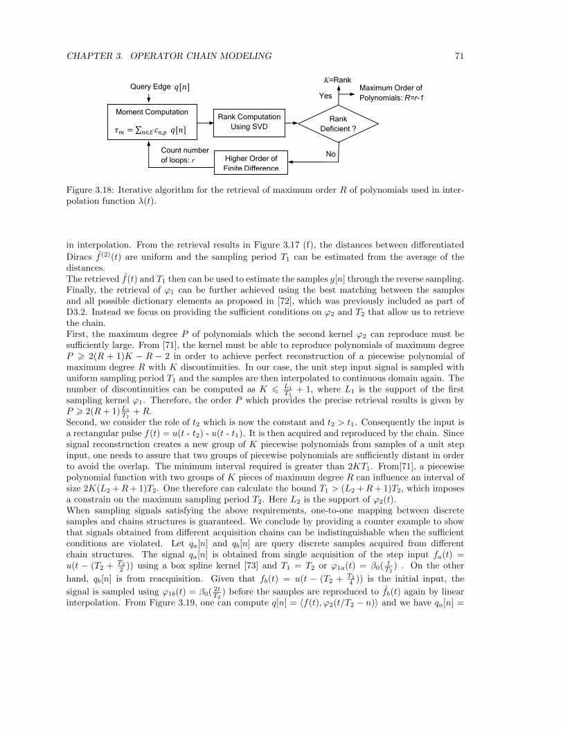
CHAPTER 3. OPERATOR CHAIN MODELING 71
,
Moment Computation
Rank Computation or SVD
Rank Deficient ?
K = 1?
Yes
No
Single Capture
Multiple Capture
Higher Order of Finite Difference
Count number of loops: r
Yes
No
Maximum Order of Polynomials: R
Query Edge
Rank Computation Using SVD
Rank Deficient ?
Higher Order of Finite Difference
Count number of loops: r
Yes
No
Maximum Order of Polynomials: R=r-1
Query Edge
Moment Computation
∑ ,
K=Rank
Figure 3.18: Iterative algorithm for the retrieval of maximum order R of polynomials used in inter-polation function λ(t).
in interpolation. From the retrieval results in Figure 3.17 (f), the distances between differentiated
Diracs f (2)(t) are uniform and the sampling period T1 can be estimated from the average of thedistances.The retrieved f(t) and T1 then can be used to estimate the samples g[n] through the reverse sampling.Finally, the retrieval of ϕ1 can be further achieved using the best matching between the samplesand all possible dictionary elements as proposed in [72], which was previously included as part ofD3.2. Instead we focus on providing the sufficient conditions on ϕ2 and T2 that allow us to retrievethe chain.First, the maximum degree P of polynomials which the second kernel ϕ2 can reproduce must besufficiently large. From [71], the kernel must be able to reproduce polynomials of maximum degreeP > 2(R + 1)K − R − 2 in order to achieve perfect reconstruction of a piecewise polynomial ofmaximum degree R with K discontinuities. In our case, the unit step input signal is sampled withuniform sampling period T1 and the samples are then interpolated to continuous domain again. Thenumber of discontinuities can be computed as K 6 L1
T1+ 1, where L1 is the support of the first
sampling kernel ϕ1. Therefore, the order P which provides the precise retrieval results is given byP > 2(R+ 1)L1
T1+R.
Second, we consider the role of t2 which is now the constant and t2 > t1. Consequently the input isa rectangular pulse f(t) = u(t - t2) - u(t - t1). It is then acquired and reproduced by the chain. Sincesignal reconstruction creates a new group of K piecewise polynomials from samples of a unit stepinput, one needs to assure that two groups of piecewise polynomials are sufficiently distant in orderto avoid the overlap. The minimum interval required is greater than 2KT1. From[71], a piecewisepolynomial function with two groups of K pieces of maximum degree R can influence an interval ofsize 2K(L2 +R+ 1)T2. One therefore can calculate the bound T1 > (L2 +R+ 1)T2, which imposesa constrain on the maximum sampling period T2. Here L2 is the support of ϕ2(t).When sampling signals satisfying the above requirements, one-to-one mapping between discretesamples and chains structures is guaranteed. We conclude by providing a counter example to showthat signals obtained from different acquisition chains can be indistinguishable when the sufficientconditions are violated. Let qa[n] and qb[n] are query discrete samples acquired from differentchain structures. The signal qa[n] is obtained from single acquisition of the step input fa(t) =u(t − (T2 + T2
2 )) using a box spline kernel [73] and T1 = T2 or ϕ1a(t) = β0( tT2
) . On the other
hand, qb[n] is from reacquisition. Given that fb(t) = u(t − (T2 + T2
4 )) is the initial input, the
signal is sampled using ϕ1b(t) = β0( 2tT2
) before the samples are reproduced to fb(t) again by linearinterpolation. From Figure 3.19, one can compute q[n] = 〈f(t), ϕ2(t/T2 − n)〉 and we have qa[n] =

CHAPTER 3. OPERATOR CHAIN MODELING 72
Additional Examples
/
012 1
12 0
0
1
3 /2 0 2 3 4 6
Figure 3.19: Counter examples when sampling fa(t) and fb(t) with a sampling kernel ϕ(t) = β0( tT2
)
qb[n] = [0 12 1 1
2 0]. The signals from different chains become indistinguishable because the kernelsused can reproduce polynomials up to degree P=0 which violates the condition. Thus one-to-onemapping is not guaranteed and the proposed algorithm cannot retrieve unique chain solution.
3.4.4 Conclusions
We have presented a theoretical scheme for the retrieval of a signal acquisition chain. With thetheory of sampling signals with FRI, we are able to classify discrete samples from different stages inthe chain model and create reacquisition detection algorithm. In addition, the method allows us todevelop a retrieval algorithm for important parameters in the reacquisition chain. We finally havediscussed the sufficient conditions to the retrieval of the parameters of the acquisition chain.
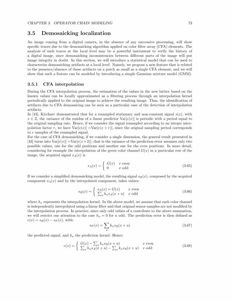
CHAPTER 3. OPERATOR CHAIN MODELING 73
3.5 Demosaicking localization
An image coming from a digital camera, in the absence of any successive processing, will showspecific traces due to the demosaicking algorithm applied on color filter array (CFA) elements. Theanalysis of such traces at the local level may be a powerful instrument to verify the history ofa digital image, since demosaicking inconsistencies between different parts of the image will putimage integrity in doubt. In this section, we will introduce a statistical model that can be used tocharacterize demosaicking artifacts at a local level. Namely, we propose a new feature that is relatedto the presence/absence of these artifacts on a patch as small as a single CFA element, and we willshow that such a feature can be modeled by introducing a simple Gaussian mixture model (GMM).
3.5.1 CFA interpolation
During the CFA interpolation process, the estimation of the values in the new lattice based on theknown values can be locally approximated as a filtering process through an interpolation kernelperiodically applied to the original image to achieve the resulting image. Thus, the identification ofartifacts due to CFA demosaicing can be seen as a particular case of the detection of interpolationartifacts.In [43], Kirchner demonstrated that for a resampled stationary and non-constant signal s(x), withx ∈ Z, the variance of the residue of a linear predictor Var[e(x)] is periodic with a period equal tothe original sampling rate. Hence, if we consider the signal resampled according to an integer inter-polation factor r, we have Var[e(x)] =Var[e(x+ r)], since the original sampling period correspondsto r samples of the resampled signal.For the case of CFA demosaicking, if we consider a single dimension, the general result presented in[43] turns into Var[e(x)] =Var[e(x+2)], that is the variance of the prediction error assumes only twopossible values, one for the odd positions and another one for the even positions. In more detail,considering for example the interpolation of the green color channel G(x) in a particular row of theimage, the acquired signal sA(x) is
sA(x) =
{G(x) x even0 x odd
(3.65)
If we consider a simplified demosaicking model, the resulting signal sR(x), composed by the acquiredcomponent sA(x) and by the interpolated component, takes values:
sR(x) =
{sA(x) = G(x) x even∑u husA(x+ u) x odd
(3.66)
where hu represents the interpolation kernel. In the above model, we assume that each color channelis independently interpolated using a linear filter and that original sensor samples are not modified bythe interpolation process. In practice, since only odd values of u contribute to the above summation,we will restrict our attention to the case hu = 0 for u odd. The prediction error is then defined ase(x) = sR(x)− sP (x), with:
sP (x) =∑u
kusR(x+ u) (3.67)
the predicted signal, and ku the prediction kernel. Hence:
e(x) =
{G(x)−∑u kusR(x+ u) x even∑u husA(x+ u)−∑u kusR(x+ u) x odd
(3.68)

CHAPTER 3. OPERATOR CHAIN MODELING 74
By assuming to use the same kernel for the interpolation and the prediction (i.e. hu = ku), theprediction error in odd positions is identically zero, while in the even positions takes values differentfrom zero. Hence, in such an ideal case, var[e(x)] is expected to be zero in the positions correspondingto the demosaicked signal, and different from zero in the positions corresponding to the acquiredsignal.In general, the exact interpolation coefficients may not be known, however we can assume thatku = 0 for u odd. Moreover, we can also assume
∑u ku =
∑u hu = 1, which usually holds for
common interpolation kernels. In this case, equation (3.68) above can be rewritten as
e(x) =
{G(x)−∑u ku
∑v hvG(x+ u+ v) x even∑
u(hu − ku)G(x+ u) x odd(3.69)
By assuming the acquired signal samples to be independent and identically distributed (i.i.d.) withmean µG and variance σ2
G, the mean of the prediction error can be evaluated as
E[e(x)] =
{µG − µG
∑u ku
∑v hv = 0 x even
µG (∑u hu −
∑u ku) = 0 x odd
(3.70)
whereas the variance of the prediction error is
Var[e(x)] =Var[(1−
∑u
kuh−u)G(x)
+∑t6=0
(∑u
kuht−u)G(x+ t)
]=σ2
G
[(1−
∑u
kuh−u)2 +∑t6=0
(∑u
kuht−u)2] (3.71)
for x even andVar[e(x)] = Var
[∑u
(hu − ku)G(x+ u)]
= σ2G
∑u
(hu − ku)2 (3.72)
for x odd. According to the above model, the prediction error has zero mean and variance pro-portional to the variance of the acquired signal. However, when the prediction kernel is close tothe interpolation kernel, the variance of prediction error will be much higher at the positions of theacquired pixels than at the positions of interpolated pixels.In order to extend the previous analysis to the bidimensional case, without loss of generality we willconsider as specific CFA the most frequently used Bayer’s filter mosaic, a 2×2 array having red andgreen filters for one row and green and blue filters for the other (see Fig. 3.20(a)). Furthermore,we will consider only the green channel; since the green channel is upsampled by a factor 2, for ageneric square block we have the same number of samples (and the same estimation reliability) forboth classes of pixels (either acquired or interpolated).By focusing on the green channel, the even/odd positions (i.e. acquired/interpolated samples) ofthe one-dimensional case turn into the quincunx lattice A for the acquired green values and thecomplementary quincunx lattice I for the interpolated green values (see Fig. 3.20(b)). Similar tothe one-dimensional case, we assume that in the presence of CFA interpolation the variance of theprediction error on lattice A is higher than the variance of the prediction error on lattice I, and inboth cases it is content dependent. On the contrary, when no demosaicking has been applied, thevariance of the prediction error assumes similar values on the two lattices.

CHAPTER 3. OPERATOR CHAIN MODELING 75
(a) (b)
Figure 3.20: (a) the Bayer’s filter mosaic; (b) the quincunx lattice A for the acquired green channelsand the complementary quincunx lattice I for the interpolated green channels.
3.5.2 Proposed model
The exact modeling of the prediction error would be in general tricky, since it depends on manyparameters like the content of the image and the actual demosaicking filter. However, it is possibleto consider a local function of the prediction error that can be modeled in a very simple and effectiveway. Let us suppose that s(x, y), with (x, y) ∈ Z2, is an observed image. The prediction error canbe obtained as:
e(x, y) = s(x, y)−∑u,v 6=0
ku,vs(x+ u, y + v) (3.73)
where ku,v is a bidimensional prediction filter. In the ideal case, ku,v = hu,v ∀(u, v) where hu,v isthe interpolation kernel of the demosaicking algorithm. In general, we can assume that ku,v 6= hu,v,since the in-camera demosaicking algorithm is usually unknown.Because of the local stationarity of the residue, we consider a local estimation of the variance of theprediction error from a neighborhood of either interpolated (I) or acquired (A) pixels, accordingto the pixel location. By assuming that the local stationarity of prediction error is valid in a(2K + 1) × (2K + 1) window, it is possible to define the local weighted variance of the predictionerror as:
σ2e(x, y) =
1
c
[( K∑i,j=−K
αij e2(x+ i, y + j)
)− (µe)
2]
(3.74)
where αij are suitable weights, µe =∑Ki,j=−K αij e(x + i, y + j) is a local weighted mean of the
prediction error and c = 1 −∑Ki,j=−K α
2ij is a scale factor that makes the estimator unbiased, i.e.,
E[σ2e(x, y)] =var[e(x, y)], for each pixel class. The weights αij are obtained as αij = α
′
ij/∑i,j α
′
ij
where
α′
ij =
{ W (i, j) if e(x+ i, x+ j) belongs tothe same class of e(x, y)
0 otherwise
and W (i, j) is a (2K + 1)× (2K + 1) Gaussian window with standard deviation K/2.Given a N × N image, we analyze it by considering B × B non-overlapping blocks, where B isrelated to the period of Bayer’s filter mosaic: the smallest period (and block dimension) is (2, 2),but also multiples can be adopted. The generic block in position (k, l) is denoted as Bk,l withk, l = 0, . . . , NB − 1. Each block is composed by disjoint sets of acquired and interpolated pixels,indicated as BAk,l and BIk,l , respectively. We then define the feature L:
L(k, l) = log
[GMA(k, l)
GMI(k, l)
](3.75)

CHAPTER 3. OPERATOR CHAIN MODELING 76
whereGMA(k, l) is the geometric mean of the variance of prediction errors at acquired pixel positions,defined as:
GMA(k, l) =
[ ∏i,j∈BAk,l
σ2e(i, j)
] 1|BAk,l
|
(3.76)
whereas GMI(k, l) is similarly defined for the interpolated pixels.The proposed feature L allows us to evaluate the imbalance between the local variance of predictionerrors when an image is demosaicked: indeed, in this case the local variance of the prediction errorof acquired pixels is higher than that of interpolated pixels and thus the expected value of L(k, l)is a nonzero positive amount. On the other hand, if an image is not demosaicked, this differencebetween the variance of prediction errors of acquired an interpolated pixels disappears, since thecontent can be assumed to present locally the same statistical properties, and the expected value ofL(k, l) is zero.Let M1 and M2 be the hypotheses of presence and absence of CFA artifacts, respectively. In orderto have a simple and tractable model, we assume that L(k, l) is Gaussian distributed under bothhypotheses and for any possible size B of the blocks Bk,l. For a fixed B, we can characterize ourfeature using the following conditional probability density functions:
Pr{L(k, l)|M1} = N (µ1, σ21) (3.77)
with µ1 > 0, andPr{L(k, l)|M2} = N (0, σ2
2). (3.78)
The above densities hold ∀k, l = 0, . . . , NB − 1, i.e., we assume that the parameters of the twoconditional pdfs do not change over the considered image, such that they can be globally estimated.If a demosaicked image contains some tampered regions in which CFA artifacts have been destroyed(as it may occur in a common splicing operation), both hypotheses M1 and M2 are present, thereforeL(k, l) can be modeled as a mixture of Gaussian distributions. The first component, with µ1 > 0,is due to regions in which CFA artifacts are present, whereas the second component, with µ2 =0, is due to tampered regions in which CFA artifacts have been removed. In order to estimatesimultaneously the parameters of the proposed GMM, we employ the Expectation-Maximization(EM) algorithm [74]. This is a standard iterative algorithm that estimates the mean and the varianceof the component distributions by maximizing the expected value of a complete log-likelihood functionwith respect to the distribution parameters. In our case, the EM algorithm is used to estimate onlyµ1, σ1, and σ2, since we assume µ2 = 0.
3.5.3 Validation
The results presented in this section have been obtained on a dataset consisting of 400 originalcolor images, in TIFF uncompressed format, coming from 4 different cameras (100 images for eachcamera): Canon EOS 450D, Nikon D50, Nikon D90, Nikon D7000. All cameras are equipped witha Bayer CFA, thus respecting our requirement that authentic images come from a camera leavingdemosaicking traces, but the in-camera demosaicking algorithms of such devices are unknown. Eachimage was cropped to 512 × 512 pixels, maintaining the original Bayer pattern, which has beenverified by inspecting the technical specifications of the raw image format. We will refer to such adataset as the original dataset.The first step was to verify the assumption of Gaussian distribution on L(k, l), both in the presenceand in the absence of CFA artifacts. To this end, starting from 100 images selected from the originaldataset, we have created two datasets satisfying the M1 (presence of CFA) and M2 (absence of CFA)
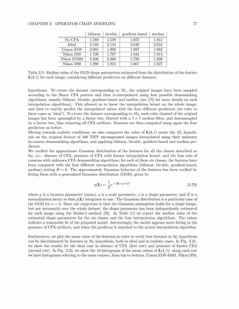
CHAPTER 3. OPERATOR CHAIN MODELING 77
bilinear bicubic gradient-based median
No CFA 1.589 1.558 1.672 1.812Ideal 2.168 2.134 2.049 2.016
Canon EOS 2.001 1.908 1.897 1.962Nikon D50 1.736 1.797 1.834 1.814
Nikon D7000 2.206 2.066 1.729 1.899Nikon D90 1.998 1.924 1.667 1.927
Table 3.5: Median value of the GGD shape parameters estimated from the distribution of the featureL(k, l) for each image, considering different predictors on different datasets.
hypotheses. To create the dataset corresponding to M1, the original images have been sampledaccording to the Bayer CFA pattern and then re-interpolated using four possible demosaickingalgorithms, namely bilinear, bicubic, gradient-based and median (see [75] for more details on suchinterpolation algorithms). This allowed us to know the interpolation kernel on the whole image,and then to exactly predict the interpolated values with the four different predictors (we refer tothese cases as ’ideal’). To create the dataset corresponding to M2, each color channel of the originalimages has been upsampled by a factor two, blurred with a 7 × 7 median filter, and downsampledby a factor two, thus removing all CFA artifacts. Features are then computed using again the fourpredictors as before.Moving towards realistic conditions, we also computed the value of L(k, l) under the M1 hypoth-esis on the original dataset of 400 TIFF uncompressed images interpolated using their unknownin-camera demosaicking algorithms, and applying bilinear, bicubic, gradient-based and median pre-dictors.We verified the approximate Gaussian distribution of the features for all the classes described sofar, i.e.: absence of CFA, presence of CFA with known interpolation kernel, and the four sets ofcameras with unknown CFA demosaicking algorithms; for each of these six classes, the features havebeen computed with the four different interpolation algorithms (bilinear, bicubic, gradient-based,median) setting B = 8. The approximately Gaussian behavior of the features has been verified byfitting them with a generalized Gaussian distribution (GGD), given by
p(L) =1
Ze−(|L−µ|/η)ν (3.79)
where µ is a location parameter (mean), η is a scale parameter, ν is a shape parameter, and Z is anormalization factor so that p(L) integrates to one. The Gaussian distribution is a particular case ofthe GGD for ν = 2. Since our conjecture is that the Gaussian assumption holds for a single image,but not necessarily over the whole dataset, the shape parameter has been independently estimatedfor each image using the Mallat’s method [76]. In Table 3.5 we report the median value of theestimated shape parameters for the six classes and the four interpolation algorithms. The valuesindicate a reasonable fit of the proposed model. Interestingly, the model appears more fitting in thepresence of CFA artifacts, and when the predictor is matched to the actual interpolation algorithm.
Furthermore, we plot the mean value of the features in order to verify how features in M1 hypothesiscan be discriminated by features in M2 hypothesis, both in ideal and in realistic cases. In Fig. 3.21,we show the results for the ideal case in absence of CFA (first row) and presence of known CFA(second row). In Fig. 3.22, we show the 16 histograms of the mean values of L(k, l): along each rowwe have histograms referring to the same camera, from top to bottom, Canon EOS 450D, Nikon D50,

CHAPTER 3. OPERATOR CHAIN MODELING 78
−30 −20 −10 0 10 20 300
0.2
0.4
0.6
0.8
1
−30 −20 −10 0 10 20 300
0.2
0.4
0.6
0.8
1
−30 −20 −10 0 10 20 300
0.2
0.4
0.6
0.8
1
−30 −20 −10 0 10 20 300
0.2
0.4
0.6
0.8
1
0 100 200 3000
0.05
0.1
0.15
0.2
0 100 200 3000
0.05
0.1
0.15
0.2
0 100 200 3000
0.05
0.1
0.15
0.2
0 100 200 3000
0.05
0.1
0.15
0.2
Figure 3.21: Distribution of the average value of L(k, l) on an image, feature evaluated on 8×8 blocks,in the absence of CFA artifacts (top row) and when the predictor is the same as the demosaickingalgorithm (bottom row), using different predictors: from left to right, bilinear (red), bicubic (blue),gradient-based (green), median (violet).
Nikon D90, Nikon D7000. For both the Figures along each column we have histograms referring tothe same predictor, from left to right, bilinear (red), bicubic (blue), gradient-based (green), median(violet).Globally, the above results confirm that the proposed features has zero mean under theM2 hypothesisand mean greater than zero under the M1 hypothesis. The histograms also highlight that the fourpredictors have different behaviors. The median predictor does not seem well suited to detect CFAartifacts, since it produces values of L(k, l) closer to zero than the other predictors, irrespective ofthe camera.

CHAPTER 3. OPERATOR CHAIN MODELING 79
−20 0 20 40 60 80 1000
0.05
0.1
0.15
0.2
−20 0 20 40 60 80 1000
0.05
0.1
0.15
0.2
−20 0 20 40 60 80 1000
0.05
0.1
0.15
0.2
−20 0 20 40 60 80 1000
0.05
0.1
0.15
0.2
−20 0 20 40 60 80 1000
0.05
0.1
0.15
0.2
−20 0 20 40 60 80 1000
0.05
0.1
0.15
0.2
−20 0 20 40 60 80 1000
0.05
0.1
0.15
0.2
−20 0 20 40 60 80 1000
0.05
0.1
0.15
0.2
−20 0 20 40 60 80 1000
0.05
0.1
0.15
0.2
−20 0 20 40 60 80 1000
0.05
0.1
0.15
0.2
−20 0 20 40 60 80 1000
0.05
0.1
0.15
0.2
−20 0 20 40 60 80 1000
0.05
0.1
0.15
0.2
−20 0 20 40 60 80 1000
0.05
0.1
0.15
0.2
−20 0 20 40 60 80 1000
0.05
0.1
0.15
0.2
−20 0 20 40 60 80 1000
0.05
0.1
0.15
0.2
−20 0 20 40 60 80 1000
0.05
0.1
0.15
0.2
Figure 3.22: Distribution of the average value of L(k, l) on an image, feature evaluated on 8 × 8blocks, with unknown in-camera demosaicking algorithms and using different predictors: along eachrow we have histograms referring to the same camera, from top to bottom, Canon EOS 450D,Nikon D50, Nikon D7000, Nikon D90; along each column we have histograms referring to the samepredictor, from left to right, bilinear (red), bicubic (blue), gradient-based (green), median (violet).

Chapter 4
Synergies with WP3 and WP4
4.1 JPEG Quantization and full-frame filtering
As introduced in Sec.3.1, we studied the DCT coefficients of a full-frame linearly filtered JPEG imageand derived an accurate mathematical analysis establishing the theoretical relationship between theDCT coefficients before and after filtering. Such theoretical framework allows to fully characterizethe probabilistic distributions of the DCT coefficients of the quantized and filtered image, givendifferent kernels. When testing the mathematical model we faced an inconsistency between thetheoretically derived models and the actual distributions of DCT coefficients of compressed filteredimages, affecting the goodness of the fit. By further investigating this incongruence, we showed thatthe DCT coefficients corresponding to different frequencies cannot be considered independent, andthose of the same frequency cannot be assumed to be i.i.d. distributed. Although in the literaturethis is a typical assumption (e.g., in [36][37][40], where it appears to be convenient and reasonable),such approximation would compromise here the conducted analysis. By considering those inter- andintra-block redundancies of the DCT coefficients in the provided analysis, we were able to redefinethe proposed theoretical model and provide an accurate mathematical framework of the consideredprocessing chain.Following we briefly recall the derived mathematical model, as described in Section 3.1 and describein details the steps taken to redefine the theoretical models taking into account the inter- andintra-block redundancy.
4.1.1 Theoretical model for the DCT coefficients of a JPEG filtered im-age.
We derive a theoretical model to describe the statistical properties of an image that has been firstJPEG compressed and then linearly filtered. In order to do that, we mathematically express thedeterministic relation between the quantized DCT coefficient dq(x, y) and those of the JPEG andfiltered image df (x, y). Recalling Sec. 3.1.2, we can express such relationship as follows:
df (x, y) = γ · dq(x, y) +N, (4.1)
where γ,N ∈ R are a scaling factor and a noise term, respectively. These two terms can be calculated,through some math, according to (4.2), where α = xmod8, β = ymod8, α′ = k1mod8, β′ = k2mod8,DCTx,y is the (x, y)-th DCT coefficient obtained from an 8×8 pixel block, IDCTx,y is the 8×8 pixel
80
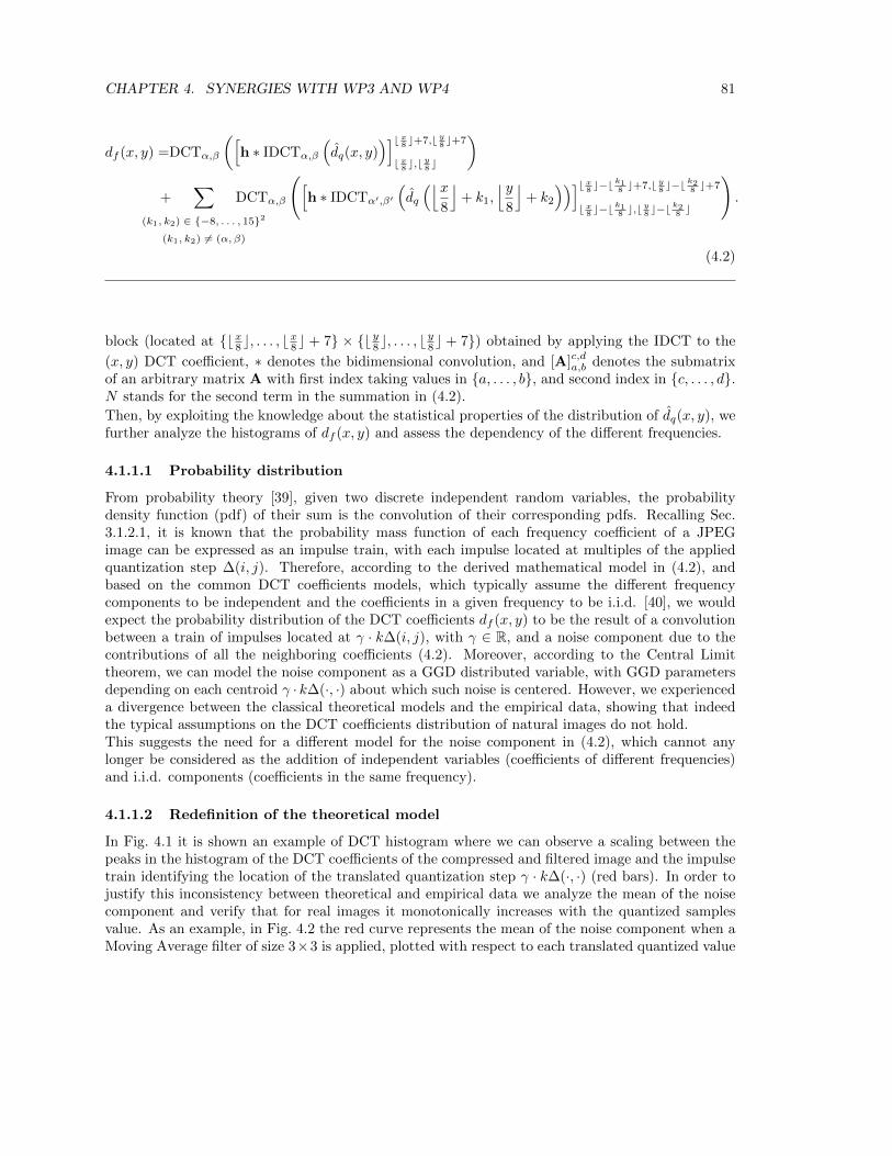
CHAPTER 4. SYNERGIES WITH WP3 AND WP4 81
df (x, y) =DCTα,β
([h ∗ IDCTα,β
(dq(x, y)
)]b x8 c+7,b y8 c+7
b x8 c,by8 c
)+
∑(k1, k2) ∈ {−8, . . . , 15}2
(k1, k2) 6= (α, β)
DCTα,β
([h ∗ IDCTα′,β′
(dq
(⌊x8
⌋+ k1,
⌊y8
⌋+ k2
))]b x8 c−b k18 c+7,b y8 c−b
k28 c+7
b x8 c−bk18 c,b
y8 c−b
k28 c
).
(4.2)
block (located at {bx8 c, . . . , bx8 c + 7} × {by8 c, . . . , by8 c + 7}) obtained by applying the IDCT to the
(x, y) DCT coefficient, ∗ denotes the bidimensional convolution, and [A]c,da,b denotes the submatrixof an arbitrary matrix A with first index taking values in {a, . . . , b}, and second index in {c, . . . , d}.N stands for the second term in the summation in (4.2).
Then, by exploiting the knowledge about the statistical properties of the distribution of dq(x, y), wefurther analyze the histograms of df (x, y) and assess the dependency of the different frequencies.
4.1.1.1 Probability distribution
From probability theory [39], given two discrete independent random variables, the probabilitydensity function (pdf) of their sum is the convolution of their corresponding pdfs. Recalling Sec.3.1.2.1, it is known that the probability mass function of each frequency coefficient of a JPEGimage can be expressed as an impulse train, with each impulse located at multiples of the appliedquantization step ∆(i, j). Therefore, according to the derived mathematical model in (4.2), andbased on the common DCT coefficients models, which typically assume the different frequencycomponents to be independent and the coefficients in a given frequency to be i.i.d. [40], we wouldexpect the probability distribution of the DCT coefficients df (x, y) to be the result of a convolutionbetween a train of impulses located at γ · k∆(i, j), with γ ∈ R, and a noise component due to thecontributions of all the neighboring coefficients (4.2). Moreover, according to the Central Limittheorem, we can model the noise component as a GGD distributed variable, with GGD parametersdepending on each centroid γ · k∆(·, ·) about which such noise is centered. However, we experienceda divergence between the classical theoretical models and the empirical data, showing that indeedthe typical assumptions on the DCT coefficients distribution of natural images do not hold.This suggests the need for a different model for the noise component in (4.2), which cannot anylonger be considered as the addition of independent variables (coefficients of different frequencies)and i.i.d. components (coefficients in the same frequency).
4.1.1.2 Redefinition of the theoretical model
In Fig. 4.1 it is shown an example of DCT histogram where we can observe a scaling between thepeaks in the histogram of the DCT coefficients of the compressed and filtered image and the impulsetrain identifying the location of the translated quantization step γ · k∆(·, ·) (red bars). In order tojustify this inconsistency between theoretical and empirical data we analyze the mean of the noisecomponent and verify that for real images it monotonically increases with the quantized samplesvalue. As an example, in Fig. 4.2 the red curve represents the mean of the noise component when aMoving Average filter of size 3×3 is applied, plotted with respect to each translated quantized value

CHAPTER 4. SYNERGIES WITH WP3 AND WP4 82
−40 −30 −20 −10 0 10 20 30 400
0.1
0.2
0.3
0.4
0.5
0.6
0.7
0.8
0.9
1
Filtered dcta kq(1,2)a kq(1,2)+meanNoise� · k�(1, 2)
� · k�(1, 2) + meanNoise
Filtered dct
Figure 4.1: Probability distribution, at frequency (1, 2), quantized with a step q(1, 2) = 10 and filtered witha 3 × 3 averaging filter. The red impulses represent the location of γ · k∆(1, 2) while the yellow ones aretranslated by the mean of the Noise component. The latter perfectly match with location of the peaks inthe histogram, thus allowing an accrue redefinition of the theoretical model fitting perfectly the empiricaldata.
γ · k∆(i, j); similar behaviors have been verified for different filter kernels. Moreover, we investigatethe verified divergence between the behavior in natural images and the theoretically modeled one, bydetermining the main causes of the noise mean component. For each coefficient df (x, y), we isolatethe contribution of each 24× 24 coefficient and analyze their influence. In Fig. 4.2 (a)-(b) we showthe specific pattern of coefficients mainly contributing to the noise, for all the AC coefficients (1, 2)and (2, 1). The red curve represents the mean of the total noise component over γ ·k∆(·, ·), the bluecurve represents the contribution of a specific set of coefficients and the black curve correspondsto the contribution of all the remaining coefficients not specified in the previous set. This set wasdetermined by isolating those coefficients that provided a significant noise contribution, in absolutevalue, over all γ · k∆(·, ·) (i.e., above an empirically determined threshold.) Note that the 24 × 24grid in the upper left part of each plot corresponds to the 9 DCT blocks taken into account in (4.1),when employing a kernel filter of size smaller than or equal to 17. The black dot identifies theconsidered frequency and the blue dots correspond to set of coefficients which mainly influence thetotal noise, as verified by the curve matching. We report only the behavior for the coefficients (1, 2)and (2, 1), but similar results are given for different frequencies.Therefore, an accurate model for the distribution of the DCT coefficients of a filtered JPEG imagecan be redefined, taking into account the scaling inferred by the noise component. In particular, thedistribution of DCT coefficients, quantized and filtered with a given kernel, will be the sum of manyGGDs, each of them centered in γ ·k∆(·, ·) translated by the mean of the noise component and withamplitude depending on the distribution of the quantized and not filtered coefficients.In Fig. 4.1 it is shown how the translated impulses, now centered in γ · k∆(·, ·) plus the mean of thenoise component, match with the peaks of the histogram.

CHAPTER 4. SYNERGIES WITH WP3 AND WP4 83
−40 −30 −20 −10 0 10 20 30 40−20
−15
−10
−5
0
5
10
15
20Coeff: (1,2)
a kq(1,2)
mea
n No
ise
TotalIndexOthers
x
� · k�(1, 2)
−40 −30 −20 −10 0 10 20 30 40−20
−15
−10
−5
0
5
10
15
20Coeff: (2,1)
a kq(2,1)
mea
n No
ise
TotalIndexOthers
x
� · k�(2, 1)
(a) (b)
Figure 4.2: Inter- and intra-block spatial redundancy affecting to df (x, y), over the entire image database.In each panel, corresponding to the frequencies (1, 2) and (2, 1), respectively (black cross in the grid in theupper left of each subplots), the total mean of the noise component (red curve) is plotted with respect tothe values of the quantized filtered coefficients γ · k∆q(i, j). The blue curve represents the contribution ofa set of coefficients (depicted in blue in the grid) and the black curve corresponds to the contribution of allthe remaining coefficients not specified in the previous set.
4.2 Transform coder identification based on quantization foot-prints and lattice theory
Transform coding has emerged over the years as the dominating compression strategy. Transformcoding is adopted in virtually all multimedia compression standards including image compressionstandards such as JPEG [77] and JPEG 2000 [78, 79] and video compression standards such as,for example, H.264/AVC [80] and HEVC [81]. This is due to the fact that transform coders arevery effective and yet computationally inexpensive since the encoding operation is divided into threerelatively simple steps: the computation of a linear transformation of the data, scalar quantizationof each coefficient, and entropy coding.Due to its centrality to any type of multimedia data, transform coding theory is now extensivelyused in a new range of applications that rely on the possibility of reverse-engineering complex chainsof operators starting from the available output signals. This has stimulated a rich set of activities inWP3, which were focused on exploiting the footprints left by single, double and multiple compression,for the case of image, video and audio signals. All these works required prior knowledge of the typeof standard being considered. This implies that the specific transform in use is assumed to be known,whereas the quantization step sizes need to be estimated. Although earlier standards (e.g., JPEG,MPEG-2 and MPEG-4) adopted the Discrete Cosine Transform (DCT) on 8×8 blocks, more recentcoding architectures addressed by the application scenarios identified in WP5 are more diversifiedin terms of both the type of transform being used and the block size. For example, JPEG2000is based on a wavelet transform that can be applied to tiles whose size can extend to the wholeimage [82]. H.264/AVC adopts an approximation of the DCT transform on 4× 4 blocks, which canbe implemented using integer arithmetic [83]. In addition, in the high-profile, H.264/AVC enablesthe adaptive choice between 4×4 and 8×8 transform block sizes. The recent HEVC standard underdevelopment goes even further, supporting four different transform block sizes in the range from4× 4 to 32× 32 [81]. The core transforms used for 4× 4 and 8× 8 are the same as in H.264/AVC,

CHAPTER 4. SYNERGIES WITH WP3 AND WP4 84
while for the two larger block sizes, integer transforms based on Chen’s fast algorithm for the DCTare used [84]. In addition, the adoption of hybrid transforms, which can be obtained by means of aseparable combination of DCT and DST (Discrete Sine Transform) is being investigated in [85]. Allthis indicates that the identification of the actual transform being used might give important cluesabout the processing history of a digital signal.Most of the methods investigated in WP3 focused only on a specific type of multimedia signal(e.g., only images or only videos) and are to some extent ad-hoc. It is therefore natural to tryand develop a universal theory of transform coder identification that is independent of the specificapplication at hand. To this end, in WP2 we considered a general model of transform coding thatcan be tailored to describe a large variety of practical implementations that are found in lossy codingsystems, including those adopted in multimedia communication. This has led to a transform coderidentification algorithm which leverages quantization footprints and lattice theory. The proposedmethod is able to successfully determine the parameters of the transform coder when a very smallnumber of vectors are observed as output of a transform coder.However, a comparison of the model adopted in WP2 with the application scenarios in WP5 (e.g.,UC-04, UC-10, etc.), reveals that, in many circumstances, signals are compressed multiple times.This provided a feedback to WP2, thus suggesting a more general model, which consists of cascadingtwo transform coders, with the goal of identifying the parameters of both of them. With respect tothe scenario addressed in Section 3.3 of this deliverable, this requires to handle noisy observation,where noise might be introduced by the quantizer of the second transform coder. Although notdescribed in this deliverable, we have obtained very promising results also along this direction,which stimulated further investigations to be continued during the third year of the project, despiteof the fact that WP2 will be officially ended.
4.3 Modeling reacquisition chains
As part of the theoretical analysis carried out in WP2 and detailed in Section 3.4 in this deliverable,we constructed a model characterising image reacquisition, as shown in Figure 4.3.Our chain model has been characterised under specific conditions. Given the assumptions of an inputbelonging to the class Finite Rate of Innovation (FRI) signals, and exponential-reproducing samplingkernels, we have shown how to recover several important parameters relative to the first unknownacquisition stage. In particular, we have shown how under these assumptions it is possible torecover the sampling period and order of the interpolator for chain structure identification, recapturedetection and the parameter retrieval, all within a completely deterministic framework.
Unit Step Input
Discrete Samples
Polynomial Interpolation
1
Sampling Kernel 1
λ(n)
1
First Acquisition
Sampling Kernel 2
Reacquisition
Figure 4.3: Image recapture model.

CHAPTER 4. SYNERGIES WITH WP3 AND WP4 85
The model developed was then applied to the practical problem of camera identification and re-capture detection of natural images. The work carried out as part of WP2 created the theoreticalfoundations upon which the practical footprint detector was then developed.However, rather than a direct implementation of the model developed, the footprint detector pre-sented in D3.2 relaxed several of the assumptions made in order to be able to operate with naturalimages. In this case, the input from natural images does not always belong to the class of FRI signalsand the sampling kernels can be of arbitrary shape. We have therefore extended the framework de-scribed in this deliverable by relaxing the assumption on sampling kernels which are now extractedfrom a dictionary of acquisition devices. The method proposed in D3.2 finds the dictionary elementswhich can best represent edge signals in a query image. While the kernel shape assumption wasrelaxed during the transition from theoretical model to practical footprint detector, the FRI signaltheory was still central to the detector developed, and the kernel dictionary was built from edgesobserved in natural images that well approximate the properties of FRI signals.Finally, the information flow is not unidirectional, as the theoretical model was adjusted and ex-panded following implementation of the footprint detector. In Figure 4.4, the connections betweenthe various components of the theoretical framework and footprint detector are highlighted. Thebackconnections from WP3 to WP2 represent the analysis of sufficient conditions for acquisitionchain retrieval whenever the input signal is an image edge, as well as the identification of the firstsampling kernel using the dictionary method outlined in D3.2.
In WP2, we setup a model for signal acquisition and develop the theoretical framework in order to describe a process carried in a chain of signal acquisition and reconstruction as presented in \figref{fig:ProblemStatement}. The chain is built with specific conditions under noise free scenario. We assume the type of input signals is a class of signals with Finite Rate of Innovation (FRI). In addition, sampling kernels used are in a specific group of kernels which can reproduce polynomials and exponentials. This allows us to describe signal using parametric expressions and to solve problems in chain structure identification, recapture detection and the parameter retrieval in deterministic way. \\ In WP3, we applied the theoretical framework to image forensics. We use the model in \figref{fig:ProblemStatement} to describe single capture and double capture of natural images. In this case, the input from natural images are not always in an FRI class and the sampling kernels can be arbitrary. We therefore, extend the framework proposed in WP2 by relaxing the assumption on sampling kernels which are now extracted from empirical acquisition devices. The method proposed in WP3 finds the dictionary elements which can best represent edge signals in a query image. Each dictionary element was built following the chain process we formulated in WP2 based on the kernels obtained from all possible known acquisition devices.
WP2
Theoretical Framework
Acquisition Model
Chain Model
FRI Analysis
Reacquisition Detection
Chain Identification
WP3
Dictionary of Edge Profiles
Edge Matching
Recapture Detection
Image Acquisition
Forensic Applications
Chain Identification
Figure 4.4: Flow of information between WP2 and WP3 contributions.
4.4 Demosaicking localization
The results obtained with the tool for the localization of color filter array (CFA) artifacts based onthe above described mathematical model indicate that the proposed method is less effective in thepresence of either almost flat areas or sharp edges. This suggests some possible directions for theextension of the above mentioned model. In the case of flat areas, we can observe that the predictionerror is almost zero irrespective of the presence of CFA artifacts. This fact appears as an intrinsic

CHAPTER 4. SYNERGIES WITH WP3 AND WP4 86
limitation of the proposed model. A more accurate model could assume that the distribution of theproposed feature is in general a mixture of two (or more) Gaussian components even in the absenceof an explicit manipulation of the CFA structure. Such components should be associated with areasof the image exhibiting similar statistical patterns. For example, different regions of the imagecould be segmented according to the variance of the content and a specific Gaussian componentcould be used to model each class. Since flat areas will be likely associated to components witha mean very close to zero, the localization of forgeries should look for local inconsistencies in themodeling of the proposed features that do not correspond to analogous inconsistencies in the localvariance of the content. In the current implementation of the tool, such an analysis is based onhuman interpretation of the forgery maps: an ambitious goal is that of devising a model permittingan automatic evaluation of such clues. Further research will be devoted to extending the currentmodels according to the above insights.On the other hand, the low performances observed in the presence of sharp edges can be ascribed tothe signal adaptive and possibly non-linear behavior of realistic in-camera demosaicking algorithms.At least in theory, such effects could be eliminated by using some prior knowledge regarding in-camera CFA interpolation, which should yield results very close to the ideal behavior foreseen bythe theoretical model. An alternative approach could be that of reverse engineering the CFA inter-polation algorithm, for example using methods such as those described in [86] to take into accounta signal adaptive behavior. However, in the presence of heavily manipulated images this approachis likely to produce a biased estimate and must be handled with care.A final observation regards the fact that detection performance is strongly affected by JPEG com-pression, limiting the applicability of the present model to scenarios in which the image under testis either uncompressed or compressed with high quality factors. Unfortunately, in this case theresults of WP3 do not offer sufficient clues about possible improvements of the current model. Fur-ther research should be devoted to assessing whether there is a fundamental limit regarding thedetectability of CFA artifacts in the presence of JPEG compression.
4.5 Double JPEG Compression Models
The experimental evaluation of the tools for the localization of image forgeries based on doubleJPEG compression statistics has offered some interesting insights on the accuracy of the relatedmathematical models. Usually, the likelihood maps produced according to the above mentionedmodels show some false alarms in image regions with either low intensity variance, like a veryuniform blue sky, or saturated values, which can occur in the presence of overexposition. As in thecase of CFA artifacts, the above behaviour suggests that the model should also take into accountthe local statistics of the image. However, in this case the extension of the current models does notappear as straightforward as in the CFA case.A very simple observation is that in the presence of flat areas we will have most of the AC DCTcoefficients quantized to zero, irrespective of the occurence of either single or double compression.This suggests to include in the model a reliability factor depending on the number of DCT coefficientshaving value equal to zero. A similar correction has been already applied in the case of the simplifiedmodel described in Section 2.2.3 of the Deliverable 2.1 and the results confirms that this is indeedbeneficial. Nevertheless, further research is needed to devise suitable strategies for incorporatinglocal image statistics in the current models.The results obtained with the developed tools also show that it is usually very difficult to separatethe distributions of singly compressed and doubly compressed DCT coefficients when the quality ofthe second compression is lower than the quality of the first one. A possible solution to overcome

CHAPTER 4. SYNERGIES WITH WP3 AND WP4 87
this problem could be that of jointly modeling the DCT coefficients of several DCT frequencies,however at the cost of a much more complex model. Moreover, as in the case of CFA artifacts, aninteresting question is whether there is some fundamental limit regarding the detectability of doubleJPEG compression. The development of such a theory will be a future research topic.
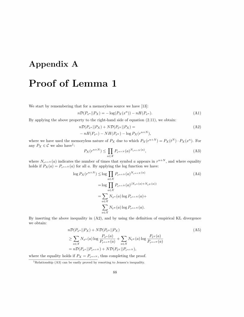
Appendix A
Proof of Lemma 1
We start by remembering that for a memoryless source we have [13]:
nD(Pxn ||PX) = − log(PX(xn))− nH(Pxn). (A1)
By applying the above property to the right-hand side of equation (2.11), we obtain:
nD(Pxn ||PX) +ND(PtN ||PX) = (A2)
− nH(Pxn)−NH(PtN )− logPX(rn+N ),
where we have used the memoryless nature of PX due to which PX(rn+N ) = PX(tN ) · PX(xn). Forany PX ∈ C we also have1:
PX(rn+N ) ≤∏a∈X
Prn+N (a)Nrn+N (a), (A3)
where Nrn+N (a) indicates the number of times that symbol a appears in rn+N , and where equalityholds if PX(a) = Prn+N (a) for all a. By applying the log function we have:
logPX(rn+N ) ≤ log∏a∈X
Prn+N (a)Nrn+N (a) (A4)
= log∏a∈X
Prn+N (a)(Nxn (a)+NtN (a))
=∑a∈X
Nxn(a) logPrn+N (a)+∑a∈X
NtN (a) logPrn+N (a).
By inserting the above inequality in (A2), and by using the definition of empirical KL divergencewe obtain:
nD(Pxn ||PX) +ND(PtN ||PX) (A5)
≥∑a∈X
Nxn(a) logPxn(a)
Prn+N (a)+∑a∈X
NtN (a) logPtN (a)
Prn+N (a)
= nD(Pxn ||Prn+N ) +ND(PtN ||Prn+N ),
where the equality holds if PX = Prn+N , thus completing the proof.
1Relationship (A3) can be easily proved by resorting to Jensen’s inequality.
88

Bibliography
[1] Harry L. van Trees, Detection, Estimation, and Modulation Theory, Wiley-Interscience, 2001.
[2] H. Vincent Poor, An Introduction to Signal Detection and Estimation, Springer, 1994.
[3] Michele A. Saad, Alan C. Bovik, and Christophe Charrier, “Blind image quality assesment: Anatural scene statistics approach in the dct domain,” IEEE Transactions on Image Processing,vol. 21, no. 8, pp. 3339–3352, August 2012.
[4] C. Cachin, “An information-theoretic model for steganography,” Information Hiding Interna-tion Workshop, vol. 1525, pp. 306–318, 1998.
[5] J. O’Brien and H. Farid, “Exposing photo manipulation with inconsistent reflections,” ACMTransactions on Graphics, vol. 1, no. 31, pp. 1–11, 2012.
[6] Rainer Bohme and Matthias Kirchner, Digital Image Forensics, chapter Counter-Forensics:Attacking Image Forensics, Springer, 2012.
[7] Martin J. Osborne and Ariel Rubinstein, A Course in Game Theory, The MIT Press, 1994.
[8] Drew Fudenberg and Jean Tirole, Game Theory, The MIT Press, 1991.
[9] M. C. Stamm, W. S. Lin, and K. J. R. Liu, “Forensics vs. anti-forensics: a decision and gametheoretic framework,” in ICASSP 2012, IEEE International Conference on Acoustics, Speechand Signal Processing, Kyoto, Japan, 25-30 March 2012.
[10] M. Barni, “A game theoretic approach to source identification with known statistics,” inICASSP 2012, IEEE International Conference on Acoustics, Speech and Signal Processing,Kyoto, Japan, 25-30 March 2012.
[11] M. J. Osborne and A. Rubinstein, A Course in Game Theory, MIT Press, 1994.
[12] M. Barni and B. Tondi, “The source identification game: an information-theoretic perspective,”submitted to IEEE Transactions on Information Forensics and Security, 2012.
[13] T. M. Cover and J. A. Thomas, Elements of Information Theory, Wiley Interscience, NewYork, 1991.
[14] I. Csiszar and J. Korner, Information Theory: Coding Theorems for Discrete MemorylessSystems. 2nd edition, Cambridge University Press, 2011.
[15] J. Nash, “Equilibrium points in n-person games,” Proceedings of the National Academy ofSciences, vol. 36, no. 1, pp. 48–49, 1950.
89

BIBLIOGRAPHY 90
[16] M. Goljan, J. Fridrich, and M. Chen, “Sensor noise camera identification: countering counterforensics,” in SPIE Conference on Media Forensics and Security, San Jose, CA, 2010.
[17] M. Gutman, “Asymptotically optimal classification for multiple tests with empirically observedstatistics,” IEEE Transactions on Information Theory, vol. 35, no. 2, pp. 401–408, March 1989.
[18] M. Kendall and S. Stuart, The Advanced Theory of Statistics, vol. 2, 4th edition, MacMillan,New York, 1979.
[19] “Special issue on digital forensics,” IEEE Signal Processing Magazing, vol. 26, no. 2, March2009.
[20] Simone Milani, Pier Francesco Piazza, Marco Tagliasacchi, and Stefano Tubaro, “An audio-video compatibility test for multimedia tampering detection,” Submitted to ACM InformationHiding and Multimedia Security 2013.
[21] Pedro Comesana, “Detection and information theoretic measures for quantifying the distin-guishability between multimedia operator chains,” in Proc. of IEEE WIFS, Tenerife, Spain,December 2012, pp. 211–216.
[22] David Slepian and Jack W. Wolf, “Noiseless coding of correlated information sources,” IEEETransactions on Information Theory, vol. 19, no. 4, pp. 471–480, July 1973.
[23] Aaron D. Wyner and Jacob Ziv, “The rate-distortion function for source coding with sideinformation at the decoder,” IEEE Transactions on Information Theory, vol. 22, no. 1, pp.1–10, January 1976.
[24] Md. Saifur Rahman and Aaron b. Wagner, “On the optimality of binning for distributedhypothesis testing,” IEEE Transactions on Information Theory, vol. 58, no. 10, pp. 6282–6303,October 2012.
[25] R. Neelamani, R. de Queiroz, Z. Fan, S. Dash, and R.G. Baraniuk, “JPEG compression historyestimation for color images,” IEEE Transactions on Image Processing, vol. 15, no. 6, pp.1365–1378, June 2006.
[26] J. Rhedi, W. Taktak, and J-L. Dugelay, “Digital image forensics: a booklet for beginners.,”Multimedia Application Tools, vol. 51, pp. 133–162, 2011.
[27] W. Luo, J. Huang, and G. Qiu;, “JPEG error analysis and its application to digital imageforensics,” IEEE Transactions on Information Forensics and Security, vol. 5, no. 3, pp. 480–491, 2010.
[28] K. Pearson, “On the criterion that a given system of deviations from the probable in the caseof correlated system of variables is such that it can be reasonably supposed to have arisen fromrandom sampling.,” Philosophical Magazine, vol. 50, pp. 157–175, 1900.
[29] D. Xu, T. Cham, S. Yan, L. Duan, and S. Chang, “Near duplicate identification with spatiallyaligned pyramid matching.,” IEEE Trans. Circuits Syst. Video Techn., vol. 20, pp. 1068–1079,2010.
[30] J. Zhang, M. Marsza lek, S. Lazebnik, and C. Schmid, “Local features and kernels for classi-fication of texture and object categories: A comprehensive study.,” International Journal ofComputer Vision, vol. 73, pp. 213–238, 2007.

BIBLIOGRAPHY 91
[31] A. Westfeld and A. Pfitzmann, “Attacks on steganographic systems - breaking the stegano-graphic utilities ezstego, jsteg, steganos, and s-toolsand some lessons learned.,” Lectures Noteson Computer Science, Springer-Verlag, vol. 1768, pp. 61–75, 2000.
[32] J. Puzicha, T. Hofmann, and J. Buhmann, “Non- parametric similarity measures for unsu-pervised texture segmen- tation and image retrieval.,” IEEE Computer Society Conference onComputer Vision and Patter Recognition (CVPR), pp. 267–272, 1997.
[33] G. Schaefer and M. Stich, “UCID - an uncompressed colour image database,” Proc. SPIE,Storage and Retrieval Methods and Applications for Multimedia, pp. 472–480, 2004.
[34] T. Bianchi, A. De Rosa, and A. Piva, “Improved dct coefficient analysis for forgery localizationin jpeg images,” in ICASSP, 2011, pp. 2444–2447.
[35] T. Bianchi and A. Piva, “Image forgery localization via block-grained analysis of JPEG arti-facts,” IEEE Transactions on Information Forensics and Security, vol. 7, no. 3, pp. 1003–1017,June 2012.
[36] Ingemar J. Cox, Digital Watermarking and Steganography, Morgan Kaufmann Publishers,2008.
[37] M. Barni and F. Bartolini, Watermarking systems engineering - Enabling digital assets securityand other applications, CRC Press, 2004.
[38] G.W. Corder and D.I. Foreman, Nonparametric Statistics for Non-Statisticians: A Step-by-Step Approach, Wiley, 2009.
[39] A. Papoulis, Probability, Random Variables and Stochastic Processes, McGraw-Hill Interna-tional Edition, 1991.
[40] Pierre Moulin and M. Kvanc Mihcak, “A framework for evaluating the data-hiding capacity ofimage sources,” IEEE Transactions on Image Processing, vol. 11, no. 9, pp. 1029–1042, 2002.
[41] A.C. Popescu and H. Farid, “Exposing digital forgeries by detecting traces of resampling,”IEEE Transactions on Signal Processing, vol. 53, no. 2, pp. 758–767, feb. 2005.
[42] B. Mahdian and S. Saic, “Blind authentication using periodic properties of interpolation,”IEEE Transactions on Information Forensics and Security, vol. 3, no. 3, pp. 529–538, sept.2008.
[43] M. Kirchner, “Fast and reliable resampling detection by spectral analysis of fixed linear pre-diction residue,” in 10th ACM Multimedia and Security Workshop (MM&Sec ’08), 2008, pp.11–20.
[44] B. Mahdian and S. Saic, “A cyclostationarity analysis applied to image forensics,” in 2009Workshop on Applications of Computer Vision (WACV), dec. 2009, pp. 1–6.
[45] D. Vazquez-Padın, C. Mosquera, and F. Perez-Gonzalez, “Two-dimensional statistical test forthe presence of almost cyclostationarity on images,” in 2010 17th IEEE Int. Conference onImage Processing (ICIP), sept. 2010, pp. 1745–1748.
[46] N. Dalgaard, C. Mosquera, and F. Perez-Gonzalez, “On the role of differentiation for resamplingdetection,” in 2010 17th IEEE Int. Conference on Image Processing (ICIP), sept. 2010, pp.1753–1756.

BIBLIOGRAPHY 92
[47] D. Vazquez-Padın and F. Perez-Gonzalez, “Prefilter design for forensic resampling estimation,”in 2011 IEEE Int. Workshop on Information Forensics and Security (WIFS), dec. 2011, pp.1–6.
[48] “Audio database,” http://opihi.cs.uvic.ca/sound/genres.tar.gz.
[49] Anil K. Jain, Fundamentals of digital image processing, Prentice-Hall, Inc., Upper Saddle River,NJ, USA, 1989.
[50] J. Lukas, J. Fridrich, and M. Goljan, “Digital camera identification from sensor pattern noise,”IEEE Transactions on Information Forensics and Security, vol. 1, no. 2, pp. 205–214, June2006.
[51] M. Chen, J. J. Fridrich, M. Goljan, and J. Lukas, “Determining image origin and integrityusing sensor noise,” IEEE Transactions on Information Forensics and Security, vol. 3, no. 1,pp. 74–90, 2008.
[52] G. Valenzise, S. Magni, M. Tagliasacchi, and S. Tubaro, “No-reference pixel video qualitymonitoring of channel-induced distortion,” IEEE Transactions on Circuits and Systems forVideo Technology, vol. 22, no. 4, pp. 605–618, 2012.
[53] M. Naccari, M. Tagliasacchi, and S. Tubaro, “No-reference video quality monitoring forH.264/AVC coded video,” IEEE Transactions on Multimedia, vol. 11, no. 5, pp. 932–946,2009.
[54] M.R. Banham and A.K. Katsaggelos, “Digital image restoration,” IEEE Signal ProcessingMagazine, vol. 14, no. 2, pp. 24–41, 1997.
[55] Z. Fan and R. L. de Queiroz, “Identification of bitmap compression history: JPEG detectionand quantizer estimation,” IEEE Transactions on Image Processing, vol. 12, no. 2, pp. 230–235,2003.
[56] J. Lukas and J. Fridrich, “Estimation of primary quantization matrix in double compressedJPEG images,” in Proc. of DFRWS, 2003.
[57] Y. Chen, K. S. Challapali, and M. Balakrishnan, “Extracting coding parameters from pre-coded MPEG-2 video,” in IEEE International Conference on Image Processing (ICIP), 1998,pp. 360–364.
[58] H. Li and S. Forchhammer, “MPEG2 video parameter and no reference PSNR estimation,” inPicture Coding Symposium (PCS), 2009, pp. 1–4.
[59] W. Luo, M. Wu, and J. Huang, “MPEG recompression detection based on block artifacts,” inSociety of Photo-Optical Instrumentation Engineers (SPIE) Conference Series, 2008, vol. 6819.
[60] W. Wang and H. Farid, “Exposing digital forgeries in video by detecting double quantization,”in Proceedings of the 11th ACM workshop on Multimedia and security, New York, NY, USA,2009, MM&Sec, pp. 39–48, ACM.
[61] M. Tagliasacchi and S. Tubaro, “Blind estimation of the QP parameter in H.264/AVC de-coded video,” in International Workshop on Image Analysis for Multimedia Interactive Services(WIAMIS), 2010, 2010, pp. 1–4.

BIBLIOGRAPHY 93
[62] P. Bestagini, A. Allam, S. Milani, M. Tagliasacchi, and S. Tubaro, “Video codec identification,”in IEEE International Conference on Acoustics, Speech, and Signal Processing (ICASSP), 2012,pp. 2257–2260.
[63] R. M. Gray and D.L. Neuhoff, “Quantization,” IEEE Transactions on Information Theory,vol. 44, no. 6, pp. 2325–2383, oct 1998.
[64] R. Zamir, S. Shamai, and U. Erez, “Nested linear/lattice coes for structured multiterminalbinning,” IEEE Transactions on Information Theory, vol. 48, no. 6, pp. 1250–1276, june 2002.
[65] D. Wubben, D. Seethaler, J. Jaldn, and G. Matz, “Lattice reduction: A survey with applicationsin wireless communications,” IEEE Signal Processing Magazine, vol. 28, no. 3, pp. 70–91, May2011.
[66] A. K. Lenstra, H. W. Lenstra, and L. Lovsz, “Factoring polynomials with rational coefficients,”Mathematische Annalen, vol. 261, pp. 515–534, 1982, 10.1007/BF01457454.
[67] J. H. Conway, N. J. A. Sloane, and E. Bannai, Sphere-packings, lattices, and groups, Springer-Verlag New York, Inc., New York, NY, USA, 1987.
[68] H. Cohen, A Course in Computational Algebraic Number Theory, vol. 138 of Graduate Textsin Mathematics, Springer, 1993.
[69] B. Gruber, “Alternative formulae for the number of sublattices,” Acta Crystallographica SectionA, vol. 53, pp. 807–808, 1997.
[70] T. Blu, P. Thevenaz, and M. Unser, “MOMS: Maximal-order interpolation of minimal support,”IEEE Transactions on Image Processing, vol. 10, no. 7, pp. 1069–1080, July 2001.
[71] P.L. Dragotti, M. Vetterli, and T. Blu, “Sampling moments and reconstructing signals of finiterate of innovation: Shannon meets Strang-Fix,” vol. 55, no. 5, pp. 1741–1757, May 2007.
[72] T. Thongkamwitoon, H. Muammar, and P.L. Dragotti, “Identification of image acquisitionchains using a dictionary of edge profiles,” pp. 1757–1761, 2012.
[73] M. Unser, A. Aldroubi, and M. Eden, “B-Spline signal processing: Part I—Theory,” IEEETransactions on Signal Processing, vol. 41, no. 2, pp. 821–833, February 1993.
[74] A. P. Dempster, N. M. Laird, and D. B. Rubin, “Maximum likelihood from incomplete datavia the EM algorithm,” Journal of the Royal Statistical Society: Series B 39, pp. 1–38, 1977.
[75] Alin C. Popescu and Hany Farid, “Exposing digital forgeries in color filter array interpolatedimage,” IEEE Transactions on Signal Processing, vol. 53, no. 10, pp. 3948–1959, 2005.
[76] S.G. Mallat, “A theory for multiresolution signal decomposition: the wavelet representation,”IEEE Transactions on Pattern Analysis and Machine Intelligence, vol. 11, no. 7, pp. 674 –693,July 1989.
[77] G.K. Wallace, “The JPEG still picture compression standard,” IEEE Transactions on Con-sumer Electronics, vol. 38, no. 1, pp. xviii–xxxiv, feb 1992.
[78] D.S. Taubman and M. W. Marcellin, JPEG 2000: Image Compression Fundamentals, Stan-dards, and Practice, Springer-Verlag, 2002.

BIBLIOGRAPHY 94
[79] D.T. Lee, “JPEG 2000: Retrospective and new developments,” Proceedings of the IEEE, vol.93, no. 1, pp. 32–41, jan 2005.
[80] G.J. Sullivan and T. Wiegand, “Video compression - from concepts to the H.264/AVC stan-dard,” Proceedings of the IEEE, vol. 93, no. 1, pp. 18–31, jan 2005.
[81] M. Winken, P. Helle, D. Marpe, H. Schwarz, and T. Wiegand, “Transform coding in theHEVC test model,” in IEEE International Conference on Image Processing (ICIP), 2011, pp.3693–3696.
[82] C. Christopoulos, A. Skodras, and T. Ebrahimi, “The JPEG2000 still image coding system: anoverview,” IEEE Transactions on Consumer Electronics, vol. 46, no. 4, pp. 1103–1127, Nov.2000.
[83] H.S. Malvar, A. Hallapuro, M. Karczewicz, and L. Kerofsky, “Low-complexity transform andquantization in H.264/AVC,” IEEE Transactions on Circuits and Systems for Video Technology,vol. 13, no. 7, pp. 598–603, July 2003.
[84] W. Chen, C. Smith, and S. Fralick, “A fast computational algorithm for the discrete cosinetransform,” IEEE Transactions on Communications, vol. 25, no. 9, pp. 1004–1009, Sept. 1977.
[85] C. Yeo, Y. H. Tan, Z. Li, and S. Rahardja, “Mode-dependent transforms for coding directionalintra prediction residuals,” IEEE Transactions on Circuits and Systems for Video Technology,vol. 22, no. 4, pp. 545–554, Apr. 2012.
[86] Ashwin Swaminathan, Min Wu, and K. J. Ray Liu, “Nonintrusive component forensics of visualsensors using output images,” IEEE Transactions on Information Forensics and Security, vol.2, no. 1, March 2007.