Deliverable 6-E: Adaptation of AURA Remote Sensing ... · Adaptation of AURA Remote Sensing...

“Focusing on education, research, and development of technology to sense and understand natural and manmade environments." Prepared By:

Michigan Tech Research Institute

of

Michigan Technological University

Deliverable 6-E: Adaptation of

AURA Remote Sensing Processing System Software to Include Additional Features and

for Commercial Readiness

Michigan Technological University

Characterization of Unpaved Road Condition Through the Use of

Remote Sensing Project Submitted version of:

June 22. 2015

Authors: Chris Roussi, [email protected] Brian White, [email protected] Joe Garbarino, [email protected]

Colin Brooks, [email protected]

Adaptation of AURA Remote Sensing Processing System Software to Include Additional Features and for Commercial Readiness ii

Table of Contents

Section I: Introduction .................................................................................................................................. 3

Section II: Image focus issues in 3D reconstructions of unpaved roads ....................................................... 3

Background ............................................................................................................................................... 3

Image Focus Metrics ................................................................................................................................. 3

Image Test ................................................................................................................................................. 4

Example Data Collection .......................................................................................................................... 6

Section III: Processing Results ................................................................................................................... 11

Section IV: Discussion ................................................................................................................................ 16

Section V: Further Potential Improvement ................................................................................................. 16

Section VI: Appendix A .............................................................................................................................. 18

Section VII: References .............................................................................................................................. 25

List of Figures and Tables

Figure 1: Test images. Unblurred (left), 2x2 Gaussian filter (center), 10x10 Gaussian filter (right) ........... 4

Table 1: Tests of several image focus metrics, with computational speeds (F-fast, M-medium, S-slow) .... 5

Figure 2: Sample images from Petersburg Rd collect, showing varying amounts of motion blur. .............. 6

Figure 3: Metrics computed on 200 images taken in sequence during the flight .......................................... 6

Figure 4: Histograms of three candidate metrics, and the closest standard distribution types...................... 7

Figure 5: Histogram showing distribution of Vollath Correlation metric on Petersburg Rd data ................ 8

Figure 6: Example of Vollath Correlation. Original image is shown on upper left and VC image (lower left). Blurred image (10x10 LPF) is shown on upper right with corresponding VC image (lower right). ............................................................................................................................... 9

Figure 7: Dense point clouds reconstructed from 16 sequential images (left) and the 12 images with VC>20 (right). .......................................................................................................................... 10

Figure 8: Image Entropy values for VC>0 (top) VC>10 (middile), and VC>20. ....................................... 11

Figure 9: Reconstructed height map using all images covering this road segment .................................... 12

Figure 10: Road cross-section through pothole, which is measured as 3cm deep (actual depth 15-20cm) 12

Figure 11: Height map of segmented road surface using focused images for reconstruction. .................... 13

Figure 12: Road cross-section using focused images. ................................................................................ 14

Figure 13: Height-map for a section of Walsh-Macon Rd. The gap in reconstruction is due to lack of images for that area. .................................................................................................................. 14

Figure 14: Comparison of using all images vs. only unblurred images in corrugation measurements. Shown are areas of true distress (left), results from using all images (center) and results using only focused images (right). ..................................................................................................... 15

Figure 15: Example of deblurring using blind deconvolution (result on right). ......................................... 16

Adaptation of AURA Remote Sensing Processing System Software to Include Additional Features and for Commercial Readiness 3

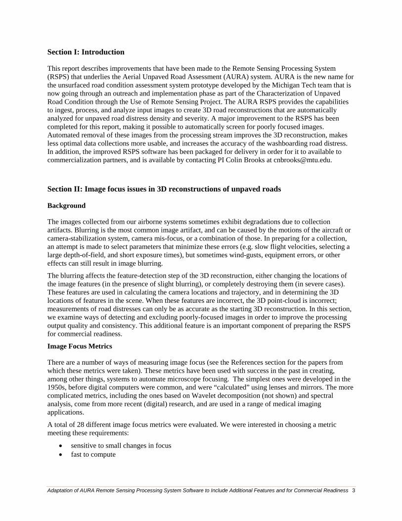
Section I: Introduction

This report describes improvements that have been made to the Remote Sensing Processing System (RSPS) that underlies the Aerial Unpaved Road Assessment (AURA) system. AURA is the new name for the unsurfaced road condition assessment system prototype developed by the Michigan Tech team that is now going through an outreach and implementation phase as part of the Characterization of Unpaved Road Condition through the Use of Remote Sensing Project. The AURA RSPS provides the capabilities to ingest, process, and analyze input images to create 3D road reconstructions that are automatically analyzed for unpaved road distress density and severity. A major improvement to the RSPS has been completed for this report, making it possible to automatically screen for poorly focused images. Automated removal of these images from the processing stream improves the 3D reconstruction, makes less optimal data collections more usable, and increases the accuracy of the washboarding road distress. In addition, the improved RSPS software has been packaged for delivery in order for it to available to commercialization partners, and is available by contacting PI Colin Brooks at [email protected].

Section II: Image focus issues in 3D reconstructions of unpaved roads

Background

The images collected from our airborne systems sometimes exhibit degradations due to collection artifacts. Blurring is the most common image artifact, and can be caused by the motions of the aircraft or camera-stabilization system, camera mis-focus, or a combination of those. In preparing for a collection, an attempt is made to select parameters that minimize these errors (e.g. slow flight velocities, selecting a large depth-of-field, and short exposure times), but sometimes wind-gusts, equipment errors, or other effects can still result in image blurring.

The blurring affects the feature-detection step of the 3D reconstruction, either changing the locations of the image features (in the presence of slight blurring), or completely destroying them (in severe cases). These features are used in calculating the camera locations and trajectory, and in determining the 3D locations of features in the scene. When these features are incorrect, the 3D point-cloud is incorrect; measurements of road distresses can only be as accurate as the starting 3D reconstruction. In this section, we examine ways of detecting and excluding poorly-focused images in order to improve the processing output quality and consistency. This additional feature is an important component of preparing the RSPS for commercial readiness.

Image Focus Metrics

There are a number of ways of measuring image focus (see the References section for the papers from which these metrics were taken). These metrics have been used with success in the past in creating, among other things, systems to automate microscope focusing. The simplest ones were developed in the 1950s, before digital computers were common, and were “calculated” using lenses and mirrors. The more complicated metrics, including the ones based on Wavelet decomposition (not shown) and spectral analysis, come from more recent (digital) research, and are used in a range of medical imaging applications.

A total of 28 different image focus metrics were evaluated. We were interested in choosing a metric meeting these requirements:

• sensitive to small changes in focus • fast to compute


• simple to code (we did not want to have to include large processing packages in the distribution, if possible)

Of the 28 metrics tested, 17 of those fit most of these requirements, and were included in our tests.

Image Test

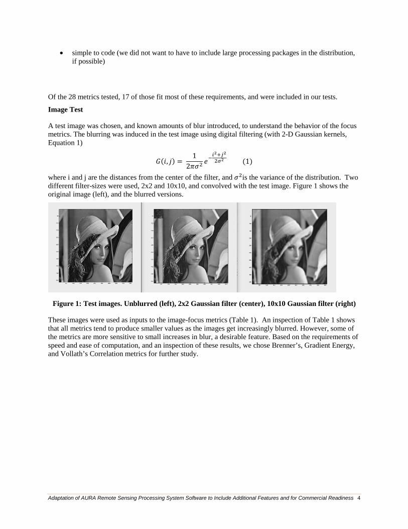
A test image was chosen, and known amounts of blur introduced, to understand the behavior of the focus metrics. The blurring was induced in the test image using digital filtering (with 2-D Gaussian kernels, Equation 1)

𝐺𝐺(𝑖𝑖, 𝑗𝑗) = 1

2𝜋𝜋𝜎𝜎2𝑒𝑒−

𝑖𝑖2+𝑗𝑗22𝜎𝜎2 (1)

where i and j are the distances from the center of the filter, and 𝜎𝜎2is the variance of the distribution. Two different filter-sizes were used, 2x2 and 10x10, and convolved with the test image. Figure 1 shows the original image (left), and the blurred versions.

Figure 1: Test images. Unblurred (left), 2x2 Gaussian filter (center), 10x10 Gaussian filter (right)

These images were used as inputs to the image-focus metrics (Table 1). An inspection of Table 1 shows that all metrics tend to produce smaller values as the images get increasingly blurred. However, some of the metrics are more sensitive to small increases in blur, a desirable feature. Based on the requirements of speed and ease of computation, and an inspection of these results, we chose Brenner’s, Gradient Energy, and Vollath’s Correlation metrics for further study.


Table 1: Tests of several image focus metrics, with computational speeds (F-fast, M-medium, S-slow)

Metric Lena Lena (2x2) Lena (10x10) Speed

Brenner’s 264 126 43 F

Contrast 54 41 21 S

Curvature 26 26 26 F

DCT energy ratio 0.043 0.039 0.022 M

DCT reduced energy ratio

0.032 0.033 0.021 M

Gaussian derivative

2.5e36 2.7e36 1.9e36 F

Graylevel variance

47.9 47.5 44.4 F

Gradient energy 267 151 41 F

Threshold gradient

8.6 6.2 3.1 F

Helmli’s mean 1.12 1.11 1.05 F

Histogram entropy

0 0 0 F

Histogram range 220 224 210 F

Laplacian energy 309.6 138.3 4.2 F

Modified Laplacian

14.2 7.3 1.1 F

Spatial Frequency

9.4 6.7 3.4 F

Tenegrad 6.9e3 6.0e3 1.5e3 F

Vollath’s correlation

62.0 48.6 14.4 F

The code that computes each of the metrics is included in Appendix A.


Example Data Collection

Some data from the Petersburg Rd campaign (collected using the Tazer single-rotor aircraft early in the first project testing year, without a camera stabilization system) were used in further testing. This dataset was chosen because of the poor results obtained both in 3D reconstruction, and in extracted results. Many of the images in this dataset were blurred, due to improper camera settings, and the hypothesis is that the poor results were due, at least in part, to the image mis-focus.

Several image fragments with a range of blurring, and a few associated metrics (Brenner’s, Gradient Energy, and Vollath’s correlation), are shown in Figure 2.

BREN = 15.3, GRAE = 39.8 , VOLA = 95.8 BREN = 8.2, GRAE = 27.5, VOLA = 53.8 BREN = 4.5, GRAE = 13.6, VOLA = 8.4

Figure 2: Sample images from Petersburg Rd collect, showing varying amounts of motion blur.

The values of these three metrics were computed on 200 images from the Petersburg Rd collect (Figure 3). The blue curve shows Brenner’s metric, the red is the Gradient Energy metric, and the yellow curve is Vollath’s Correlation.

Figure 3: Metrics computed on 200 images taken in sequence during the flight


The aircraft was in full forward flight (south-bound at 4.5mph or 2m/s) at the beginning of this collect, then slowed, hovered (around image 100), and returned. The return path shows less blurring (i.e. larger metric values), on average, than the outbound flight; this may have been due to the difference in wind buffeting (the winds were from the South at 4-12mph (1.8-5.4m/s) during that collection, and the aircraft had a head-wind on the return leg).

All metrics show similar behaviors in response to mis-focus (in that the metrics are small when mis-focus is large), but the Vollath correlation (yellow curve) shows the “best” response to well-focused images (e.g. near the middle of the collect, while hovering). It is well-known that, in an image having motion-blur, the correlation between neighboring pixels becomes higher. This motivated the development of the Vollath metric, which is a measure of local pixel correlation.

The metrics have different distributions of their values (Figure 4), when processing the same set of images. The Brenner metric (left) most closely fits a t location-scale distribution (which is characterized by having more outliers than a normal distribution); the Gradient Energy (center) is nearly Gaussian; the Vollath Correlation is very nearly log-normal.

Figure 4: Histograms of three candidate metrics, and the closest standard distribution types.

Knowing this distribution is important when choosing a threshold; the threshold on the distribution of the image metrics influences how many images get used in the reconstruction.

Consider, for example, the Vollath Correlation (VC) distribution in Figure 5. One must pick a threshold value large enough that the image has adequate focus (and, thus, does not introduce too many downstream errors in processing) while not excluding too many images (which will result in poor coverage, and gaps in the reconstruction). There is no clear threshold, and the choice depends on algorithm performance.


Figure 5: Histogram showing distribution of Vollath Correlation metric on Petersburg Rd data

This metric was applied to all 200 images in the Petersburg Rd collection, and the images examined. Qualitatively, images with a VC >20 appear to have small enough motion effects that they can be used in the reconstruction. This value also happens to be near the peak in the distribution. If VC>20 is chosen as the threshold, 28 images are excluded from the 200 available.

An in-focus example image (Figure 6, top image) was blurred with a 10x10 Gaussian low-pass filter (LPF), and the Vollath metric computed over a region of interest denoted by the yellow circle. The in-focus images are in the left column; the blurred images are in the right-hand column. It can be seen that the VC value is generally much larger, over a wider area, in the original image (lower left) versus the values in the blurred image (lower right). When the mean value over the entire image is taken, this results in a larger VC value for the in-focus image.


Figure 6: Example of Vollath Correlation. Original image is shown on upper left and VC image (lower left). Blurred image (10x10 LPF) is shown on upper right with corresponding VC image

(lower right).

Example 3D reconstructions using this metric and various threshold values are shown in Figure 7. In this case, 16 images (without regard to their focus) were used to reconstruct a small section of road (left). Then, a reconstruction spanning the same section of road was formed in which images with VC<20 were excluded (4 images excluded, right).


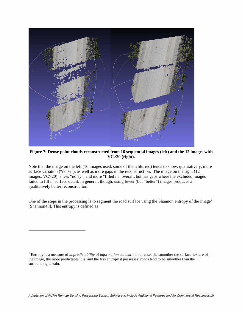
Figure 7: Dense point clouds reconstructed from 16 sequential images (left) and the 12 images with

VC>20 (right).

Note that the image on the left (16 images used, some of them blurred) tends to show, qualitatively, more surface variation (“noise”), as well as more gaps in the reconstruction. The image on the right (12 images, VC>20) is less “noisy”, and more “filled in” overall, but has gaps where the excluded images failed to fill in surface detail. In general, though, using fewer (but “better”) images produces a qualitatively better reconstruction.

One of the steps in the processing is to segment the road surface using the Shannon entropy of the image1 [Shannon48]. This entropy is defined as

1 Entropy is a measure of unpredictability of information content. In our case, the smoother the surface-texture of the image, the more predictable it is, and the less entropy it possesses; roads tend to be smoother than the surrounding terrain.


𝐸𝐸𝑖𝑖 = −�𝑝𝑝𝑖𝑖 log2 𝑝𝑝𝑖𝑖 (2)𝑘𝑘

𝑖𝑖=1

where 𝑝𝑝𝑖𝑖 contains the probability of the values in each of k = m x n regions of the image, and is given by

𝑝𝑝𝑖𝑖 = 𝐶𝐶𝐶𝐶𝐶𝐶𝐶𝐶𝐶𝐶 𝑖𝑖𝐶𝐶 𝑖𝑖𝐶𝐶ℎ ℎ𝑖𝑖𝑖𝑖𝐶𝐶𝐶𝐶𝑖𝑖𝑖𝑖𝑖𝑖𝑖𝑖 𝑏𝑏𝑖𝑖𝐶𝐶

𝑘𝑘 (3)

The relative entropy images for three cases (all images, VC>10, and VC>20) are shown in Figure 8.

Figure 8: Image Entropy values for VC>0 (top) VC>10 (middile), and VC>20.

It can be seen that the road is more “filled in” for VC>20 (which indicates more valid features were found), and the entropy values on the road surface are slightly less (about a 5% reduction in variance).

Section III: Processing Results

The standard unpaved roads processing algorithms were applied to these data. Using all the images, the results were of sufficiently poor quality that no automated results could be obtained. Examining some of the intermediate products (which are not usually used in analysis), it was clear that the road was


segmented poorly, and the height map (from which all distresses are extracted) was corrupted. The section of road that was reconstructed is shown in Figure 9.

Figure 9: Reconstructed height map using all images covering this road segment

Note that there is substantial (and unrealistic) height variation, as well as no detected potholes (even though there was a 15cm-deep pothole in the scene). An example of the road cross-section, including the pothole, is presented in Figure 10.

Figure 10: Road cross-section through pothole, which is measured as 3cm deep (actual depth 15-

20cm)


The cross-section is both “noisy”, and unrealistic. The large spike to the right of the pothole “dip” caused the automated detection algorithm to reject this as a pothole, since it did not fit the expected detection characteristics. The height map only measured the 15cm-deep pothole as 3cm.

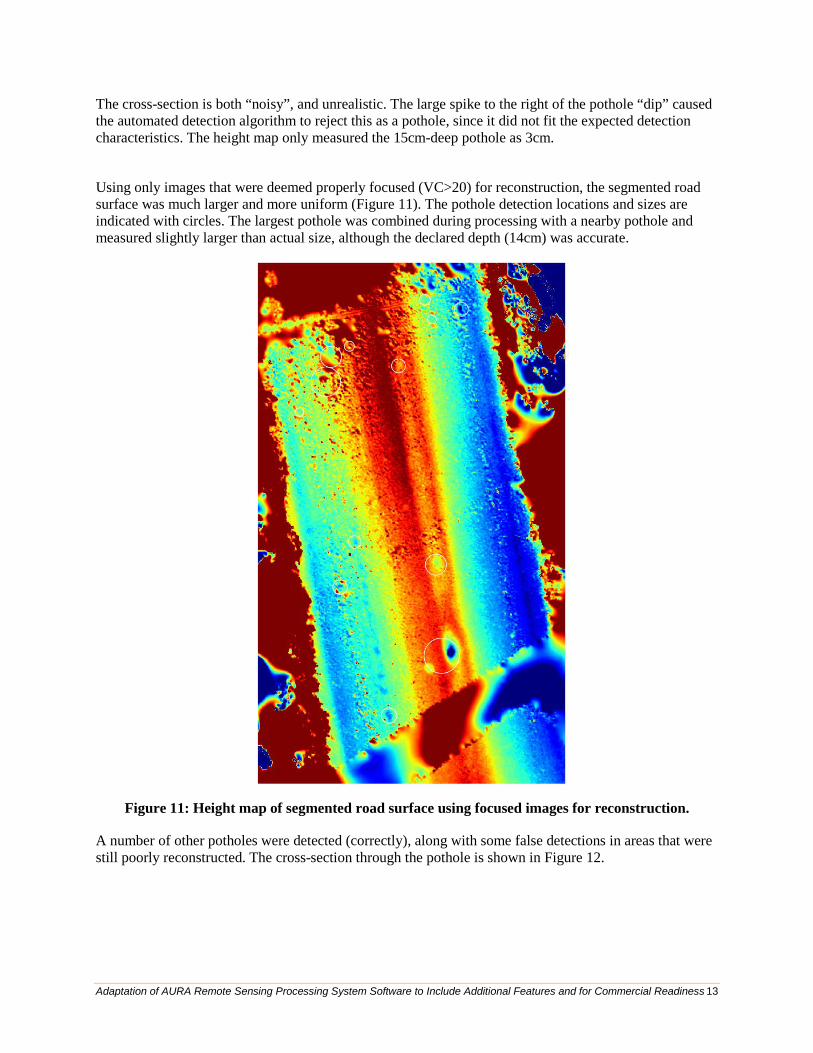
Using only images that were deemed properly focused (VC>20) for reconstruction, the segmented road surface was much larger and more uniform (Figure 11). The pothole detection locations and sizes are indicated with circles. The largest pothole was combined during processing with a nearby pothole and measured slightly larger than actual size, although the declared depth (14cm) was accurate.

Figure 11: Height map of segmented road surface using focused images for reconstruction.

A number of other potholes were detected (correctly), along with some false detections in areas that were still poorly reconstructed. The cross-section through the pothole is shown in Figure 12.


Figure 12: Road cross-section using focused images.

The height map shows much less variation on the surface, and shows clearly the road crown, and the pothole depth (14cm at this point, versus 3cm in the original measurement), which is much closer to the true value (15-20cm, depending on where it was measured).

Similar improvements have been seen with detection and classification of corrugations. The height map for a section of Walsh-Macon Road is shown in Figure 13.

Figure 13: Height-map for a section of Walsh-Macon Rd. The gap in reconstruction is due to lack

of images for that area.

Road

Edges


This section of road has a range of distresses; in some areas, the corrugations have progressed into a series of potholes, and in other areas, the corrugations have just started to form (not readily apparent in the image itself, but measurable). Ground-truth for this section of road was obtained by manual inspection. The area of the road affected by corrugations is shown on the left in Figure 14.

Figure 14: Comparison of using all images vs. only unblurred images in corrugation measurements. Shown are areas of true distress (left), results from using all images (center) and results using only

focused images (right).

The area of the road affected is 56.3 m2 of the 117.3 m2 total. When using all 18 images from this collection are used, the software classifies 75.7 m2 as corrugation (center image), a correct classification of 71%. Other areas are misclassified with a probability of 0.58. When slightly blurred images are not used in the reconstruction of the height-map (3 images were rejected), the classification is shown on the right. It is correctly classifying 94% of the corrugations, while still misclassifying about the same amount as before. This improvement in correct classification is due entirely to the use of only high-quality images in the reconstruction of the height-map; all other processing was held the same in this example. This significant improvement in corrugation classification is an important component of improving commercial readiness of the Remote Sensing Processing System.

It is worth noting that some of the poor performance in classifying corrugations that was reported earlier was due to improper ground-truth classification; the people scoring the road surface were untrained, and not following the proper procedures. With correct ground-truth, the performance is better, but improves even more with just the simple change of accepting only highly-focused images into the processing chain.


Section IV: Discussion

Tests on two datasets (Petersburg Rd and Piotr Rd) that had performed poorly show that this was due to the inclusion of poorly-focused images in the reconstruction step. The presence of blurred images degraded the 3D reconstruction, resulting in downstream algorithm failure. A method of measuring mis-focus (the Vollath Correlation metric) was implemented.

Using the Vollath Correlation image metric to find blurred images, and excluding them, results in a significantly better 3D reconstruction, and correspondingly better algorithm performance. Results were examined from an earlier dataset (Petersburg Road, collected in October 2012), which had been completely unusable before excluding blurred images. The improvement in the quality of the reconstruction was visually apparent, and easily measured using the entropy metric used for road-surface segmentation. Potholes were detected and accurately characterized, as was the crown cross-section and road width. Reprocessing a section of Walsh-Macon Road resulted in an improvement of correct corrugation classification from 71% to 94%, excluding only 3 images from the set of 18 originally used. False classifications remained about the same after reprocessing.

Although performance can be much better when blurred images are rejected, excluding too many images is undesirable. In those datasets in which there are large numbers of blurred images, the coverage of the each point on the road can drop below the minimum required (>4 images containing the same feature), and the reconstruction will fail. The application of this pre-processing stage is best suited for those datasets in which there are fewer than 25% rejected images, and those are not clustered together.

Section V: Further Potential Improvement

An alternative to detecting and excluding poorly focused images is to correct the image mis-focus. The blur can be considered to have been caused by convolving the focused image with an unknown blurring kernel, often called a “Point Spread Function” (PSF). The process of recovering and removing this unknown PSF is called “blind deconvolution”. [Katsaggelos91, Ayers88]. This problem is very ill-posed, and singular (there are an infinite number of possible solutions). A process called “regularization” is required to find a solution.

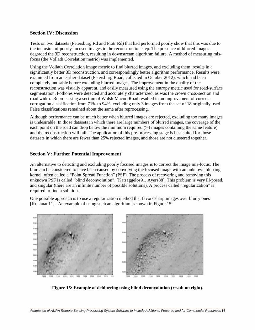
One possible approach is to use a regularization method that favors sharp images over blurry ones [Krishnan11]. An example of using such an algorithm is shown in Figure 15.

Figure 15: Example of deblurring using blind deconvolution (result on right).


The original motion-blurred image (of a pothole) is seen on the left. It would be rejected for use in 3D reconstruction, based on the degree of mis-focus. The de-blurred image is shown on the right. The Vollath Correlation for the corrected image is a factor of 10 better, resulting in an image that can be used in 3D reconstruction.

An approach such as this could be used to allow the inclusion of images that would otherwise not be useable. The drawback is that this method is computationally intensive, and would increase the overall processing time for a collection. The inclusion of this algorithm, or one like it, would be a valuable addition to the process.


Section VI: Appendix A

MATLAB code for computing candidate image focus metrics.

function FM = fmeasure(Image, Measure, ROI)

%This function measures the relative degree of focus of

%an image. It may be invoked as:

%

% FM = fmeasure(Image, Method, ROI)

%

%Where

% Image is a grayscale image and FM is the computed

% focus value.

% Method is the focus measure algorithm as a string.

%

% ROI Image ROI is a rectangle [xo yo width heigth].

% If an empty argument is passed, the whole

% image is processed.

%

% Derived from code provided by Said Pertuz

% (Intelligent Robotics and Computer Vision Group)

% (Department of Computer Science and Mathematics.)

% (Universitat Rovira i Virgili.)

%

% http://www.mathworks.com/matlabcentral/fileexchange/27314-focus- % measure/content/fmeasure/fmeasure.m

if ~isempty(ROI)

Image = imcrop(Image, ROI);

end

WSize = 15; % Size of local window (only some operators)

switch upper(Measure)

case 'ACMO' % Absolute Central Moment (Shirvaikar2004)

if ~isinteger(Image), Image = im2uint8(Image);

end

FM = AcMomentum(Image);

case 'BREN' % Brenner's (Santos97)


[M N] = size(Image);

DH = Image;

DV = Image;

DH(1:M-2,:) = diff(Image,2,1);

DV(:,1:N-2) = diff(Image,2,2);

FM = max(DH, DV);

FM = FM.^2;

FM = mean2(FM);

case 'CONT' % Image contrast (Nanda2001)

ImContrast = inline('sum(abs(x(:)-x(5)))');

FM = nlfilter(Image, [3 3], ImContrast);

FM = mean2(FM);

case 'CURV' % Image Curvature (Helmli2001)

if ~isinteger(Image), Image = im2uint8(Image);

end

M1 = [-1 0 1;-1 0 1;-1 0 1];

M2 = [1 0 1;1 0 1;1 0 1];

P0 = imfilter(Image, M1, 'replicate', 'conv')/6;

P1 = imfilter(Image, M1', 'replicate', 'conv')/6;

P2 = 3*imfilter(Image, M2, 'replicate', 'conv')/10 ...

-imfilter(Image, M2', 'replicate', 'conv')/5;

P3 = -imfilter(Image, M2, 'replicate', 'conv')/5 ...

+3*imfilter(Image, M2, 'replicate', 'conv')/10;

FM = abs(P0) + abs(P1) + abs(P2) + abs(P3);

FM = mean2(FM);

case 'DCTE' % DCT energy ratio (Shen2006)

FM = nlfilter(Image, [8 8], @DctRatio);

FM = mean2(FM);

case 'DCTR' % DCT reduced energy ratio (Lee2009)

FM = nlfilter(Image, [8 8], @ReRatio);

FM = mean2(FM);

case 'GDER' % Gaussian derivative (Geusebroek2000)

N = floor(WSize/2);

sig = N/2.5;

[x,y] = meshgrid(-N:N, -N:N);


G = exp(-(x.^2+y.^2)/(2*sig^2))/(2*pi*sig);

Gx = -x.*G/(sig^2);Gx = Gx/sum(Gx(:));

Gy = -y.*G/(sig^2);Gy = Gy/sum(Gy(:));

Rx = imfilter(double(Image), Gx, 'conv', 'replicate');

Ry = imfilter(double(Image), Gy, 'conv', 'replicate');

FM = Rx.^2+Ry.^2;

FM = mean2(FM);

case 'GLVA' % Graylevel variance (Krotkov86)

FM = std2(Image);

case 'GLLV' %Graylevel local variance (Pech2000)

LVar = stdfilt(Image, ones(WSize,WSize)).^2;

FM = std2(LVar)^2;

case 'GLVN' % Normalized GLV (Santos97)

FM = std2(Image)^2/mean2(Image);

case 'GRAE' % Energy of gradient (Subbarao93)

Ix = Image;

Iy = Image;

Iy(1:end-1,:) = diff(Image, 1, 1);

Ix(:,1:end-1) = diff(Image, 1, 2);

FM = Ix.^2 + Iy.^2;

FM = mean2(FM);

case 'GRAT' % Thresholded gradient (Snatos97)

Th = 0; %Threshold

Ix = Image;

Iy = Image;



FM = max(abs(Ix), abs(Iy));

FM(FM<Th)=0;

FM = sum(FM(:))/sum(sum(FM~=0));

case 'GRAS' % Squared gradient (Eskicioglu95)

Ix = diff(Image, 1, 2);

FM = Ix.^2;

FM = mean2(FM);


case 'HELM' %Helmli's mean method (Helmli2001)

MEANF = fspecial('average',[WSize WSize]);

U = imfilter(Image, MEANF, 'replicate');

R1 = U./Image;

R1(Image==0)=1;

index = (U>Image);

FM = 1./R1;

FM(index) = R1(index);

FM = mean2(FM);

case 'HISE' % Histogram entropy (Krotkov86)

FM = entropy(Image);

case 'HISR' % Histogram range (Firestone91)

FM = max(Image(:))-min(Image(:));

case 'LAPE' % Energy of laplacian (Subbarao93)

LAP = fspecial('laplacian');

FM = imfilter(Image, LAP, 'replicate', 'conv');

FM = mean2(FM.^2);

case 'LAPM' % Modified Laplacian (Nayar89)

M = [-1 2 -1];

Lx = imfilter(Image, M, 'replicate', 'conv');

Ly = imfilter(Image, M', 'replicate', 'conv');

FM = abs(Lx) + abs(Ly);

FM = mean2(FM);

case 'LAPV' % Variance of laplacian (Pech2000)

LAP = fspecial('laplacian');

ILAP = imfilter(Image, LAP, 'replicate', 'conv');

FM = std2(ILAP)^2;

case 'LAPD' % Diagonal laplacian (Thelen2009)

M1 = [-1 2 -1];

M2 = [0 0 -1;0 2 0;-1 0 0]/sqrt(2);

M3 = [-1 0 0;0 2 0;0 0 -1]/sqrt(2);

F1 = imfilter(Image, M1, 'replicate', 'conv');




F4 = imfilter(Image, M1', 'replicate', 'conv');

FM = abs(F1) + abs(F2) + abs(F3) + abs(F4);

FM = mean2(FM);

case 'SFIL' %Steerable filters (Minhas2009)

% Angles = [0 45 90 135 180 225 270 315];

N = floor(WSize/2);

sig = N/2.5;

[x,y] = meshgrid(-N:N, -N:N);

G = exp(-(x.^2+y.^2)/(2*sig^2))/(2*pi*sig);

Gx = -x.*G/(sig^2);Gx = Gx/sum(Gx(:));

Gy = -y.*G/(sig^2);Gy = Gy/sum(Gy(:));

R(:,:,1) = imfilter(double(Image), Gx, 'conv', 'replicate');

R(:,:,2) = imfilter(double(Image), Gy, 'conv', 'replicate');

R(:,:,3) = cosd(45)*R(:,:,1)+sind(45)*R(:,:,2);

R(:,:,4) = cosd(135)*R(:,:,1)+sind(135)*R(:,:,2);

R(:,:,5) = cosd(180)*R(:,:,1)+sind(180)*R(:,:,2);

R(:,:,6) = cosd(225)*R(:,:,1)+sind(225)*R(:,:,2);

R(:,:,7) = cosd(270)*R(:,:,1)+sind(270)*R(:,:,2);

R(:,:,7) = cosd(315)*R(:,:,1)+sind(315)*R(:,:,2);

FM = max(R,[],3);

FM = mean2(FM);

case 'SFRQ' % Spatial frequency (Eskicioglu95)

Ix = Image;

Iy = Image;



FM = mean2(sqrt(double(Iy.^2+Ix.^2)));

case 'TENG'% Tenengrad (Krotkov86)

Sx = fspecial('sobel');

Gx = imfilter(double(Image), Sx, 'replicate', 'conv');

Gy = imfilter(double(Image), Sx', 'replicate', 'conv');

FM = Gx.^2 + Gy.^2;

FM = mean2(FM);

case 'TENV' % Tenengrad variance (Pech2000)


Sx = fspecial('sobel');

Gx = imfilter(double(Image), Sx, 'replicate', 'conv');

Gy = imfilter(double(Image), Sx', 'replicate', 'conv');

G = Gx.^2 + Gy.^

FM = std2(G)^2;

case 'VOLA' % Vollath's correlation (Santos97)

Image = double(Image);

I1 = Image; I1(1:end-1,:) = Image(2:end,:);

I2 = Image; I2(1:end-2,:) = Image(3:end,:);

Image = Image.*(I1-I2);

FM = mean2(Image);

case 'WAVS' %Sum of Wavelet coeffs (Yang2003)

[C,S] = wavedec2(Image, 1, 'db6');

H = wrcoef2('h', C, S, 'db6', 1);

V = wrcoef2('v', C, S, 'db6', 1);

D = wrcoef2('d', C, S, 'db6', 1);

FM = abs(H) + abs(V) + abs(D);

FM = mean2(FM);

case 'WAVV' %Variance of Wav...(Yang2003)


H = abs(wrcoef2('h', C, S, 'db6', 1));

V = abs(wrcoef2('v', C, S, 'db6', 1));

D = abs(wrcoef2('d', C, S, 'db6', 1));

FM = std2(H)^2+std2(V)+std2(D);

case 'WAVR'


H = abs(wrcoef2('h', C, S, 'db6', 1));

V = abs(wrcoef2('v', C, S, 'db6', 1));

D = abs(wrcoef2('d', C, S, 'db6', 1));

A1 = abs(wrcoef2('a', C, S, 'db6', 1))

A2 = abs(wrcoef2('a', C, S, 'db6', 2));

A3 = abs(wrcoef2('a', C, S, 'db6', 3));

A = A1 + A2 + A3;

WH = H.^2 + V.^2 + D.^2;

WH = mean2(WH);

WL = mean2(A);


FM = WH/WL;

otherwise

error('Unknown measure %s',upper(Measure))

end

end %**********************************************************************

function fm = AcMomentum(Image)

[M N] = size(Image);

Hist = imhist(Image)/(M*N);

Hist = abs((0:255)-255*mean2(Image))'.*Hist;

fm = sum(Hist);

end

%******************************************************************

function fm = DctRatio(M)

MT = dct2(M).^2;

fm = (sum(MT(:))-MT(1,1))/MT(1,1);

end

%**********************************************************************

function fm = ReRatio(M)

M = dct2(M);

fm = (M(1,2)^2+M(1,3)^2+M(2,1)^2+M(2,2)^2+M(3,1)^2)/(M(1,1)^2);

end

%******************************************************************


Section VII: References

[Ayers88] G. R. Ayers and J. C. Dainty. Interative blind deconvolution method and its applications. Opt. Lett., 1988.

[Eskicioglu95] A.M. Eskicioglu and P.S. Fisher, “ Image quality measures and their performance”, IEEE Trans. Commun., vol.43, pp. 2959-2965, Dec. 1995.

[Katsaggelos91] A. K. Katsaggelos and K. T. Lay. Maximum likelihood blur identification and image restoration using the em algorithm. IEEE Trans. Signal Processing, 1991.

[Krishnan11] D. Krishnan, T. Tay, R. Fergus, "Blind deconvolution using a normalized sparsity measure", CVPR, 2011, 2013 IEEE Conference on Computer Vision and Pattern Recognition, 2013 IEEE Conference on Computer Vision and Pattern Recognition 2011, pp. 233-240, doi:10.1109/CVPR.2011.5995521

[Krotkov87] Krotkov, E. (1987) Focusing. Int. J. Computer Vision, 1, 223–237. Mendelsohn, M.L. & Mayall, B.H. (1972) Computer-oriented analysis of human chromosomes – III focus. Comput. Biol. Med. 2, 137.

[Nanda2001] H. Nanda, R. Cutler, Practical calibrations for a real-time digital omnidirectional camera, Technical Report, Technical Sketches, Computer Vision and Pattern Recognition, 2001.

[Nayar94] S. Nayar, Y. Nakagawa, Shape from focus, IEEE Trans. Pattern Analysis and Machine Intelligence 16 (1994) 824–831.

[Santos97] A. Santos, C. O. de Solorzano, J. J. Vaquero, J. M. Pena, N. Mapica, F. D. Pozo, Evaluation of autofocus functions in moleclar cytogenetic analysis, Journal of Microscopy 188 (1997) 264–272.

[Shannon48] Shannon, Claude E. (July–October 1948). "A Mathematical Theory of Communication". Bell System Technical Journal 27 (3): 379–423. doi:10.1002/j.1538-7305.1948.tb01338.x.

[Subbarao93] M. Subbarao, T. Choi, and A. Nikzad, “Focusing Techniques,” J. Optical Eng., vol. 32, no. 11, pp. 2,824-2,836, Nov. 1993.

[Subbarao95] M. Subbarao, T. Choi, Accurate recovery of three-dimensional shape from image focus, IEEE Trans. Pattern Analysis and Machine Intelligence 17 (1995) 266–274.

[Subbarao98] M. Subbarao, J. K. Tian, Selecting the optimal focus measure for autofocusing and depth-from-focus, IEEE Trans. Pattern Analysis and Machine Intelligence 20 (1998) 864–870.

[Thiebaut95] E. Thiebaut and J.-M. Conan. Strict a priori constraints for maximum-likelihood blind deconvolution. J. Opt. Soc. Am. A, 12(3):485–492, 1995.

[Vollath88] Vollath, D. (1988) The influence of the scene parameters and of noise on the behaviour of automatic focusing algorithms. J. Microsc. 151, 133–146.

https://en.wikipedia.org/wiki/A_Mathematical_Theory_of_Communication

https://en.wikipedia.org/wiki/Digital_object_identifier

https://dx.doi.org/10.1002%2Fj.1538-7305.1948.tb01338.x

Deliverable 6-E: Adaptation of AURA Remote Sensing ... · Adaptation of AURA Remote Sensing...

Documents

Transcript of Deliverable 6-E: Adaptation of AURA Remote Sensing ... · Adaptation of AURA Remote Sensing...