Delft University of Technology Non-Intrusive ...

Delft University of Technology

Non-Intrusive Characterization and Monitoring of Fluid MudLaboratory Experiments with Seismic Techniques, Distributed Acoustic Sensing (DAS),and Distributed Temperature Sensing (DTS)Draganov, D.S.; Ma, X.; Buisman, M.; Kiers, Tjeerd ; Heller, H.K.J.; Kirichek, Alex

DOI10.5772/intechopen.98420Publication date2021Document VersionFinal published versionPublished inSediment Transport - Recent Advances

Citation (APA)Draganov, D. S., Ma, X., Buisman, M., Kiers, T., Heller, H. K. J., & Kirichek, A. (2021). Non-IntrusiveCharacterization and Monitoring of Fluid Mud: Laboratory Experiments with Seismic Techniques, DistributedAcoustic Sensing (DAS), and Distributed Temperature Sensing (DTS). In A. J. Manning (Ed.), SedimentTransport - Recent Advances IntechOpen. https://doi.org/10.5772/intechopen.98420Important noteTo cite this publication, please use the final published version (if applicable).Please check the document version above.

CopyrightOther than for strictly personal use, it is not permitted to download, forward or distribute the text or part of it, without the consentof the author(s) and/or copyright holder(s), unless the work is under an open content license such as Creative Commons.

Takedown policyPlease contact us and provide details if you believe this document breaches copyrights.We will remove access to the work immediately and investigate your claim.

This work is downloaded from Delft University of Technology.For technical reasons the number of authors shown on this cover page is limited to a maximum of 10.

https://doi.org/10.5772/intechopen.98420

https://doi.org/10.5772/intechopen.98420

Chapter

Non-Intrusive Characterizationand Monitoring of Fluid Mud:Laboratory Experiments withSeismic Techniques, DistributedAcoustic Sensing (DAS), andDistributed Temperature Sensing(DTS)Deyan Draganov, Xu Ma, Menno Buisman,Tjeerd Kiers,

Karel Heller and Alex Kirichek

Abstract

In ports and waterways, the bathymetry is regularly surveyed for updatingnavigation charts ensuring safe transport. In port areas with fluid-mud layers, mosttraditional surveying techniques are accurate but are intrusive and provide one-dimensional measurements limiting their application. Current non-intrusive sur-veying techniques are less accurate in detecting and monitoring muddy consoli-dated or sandy bed below fluid-mud layers. Furthermore, their application isrestricted by surveying-vessels availability limiting temporary storm- or dredging-related bathymetrical changes capture. In this chapter, we first review existing non-intrusive techniques, with emphasis on sound techniques. Then, we give a shortreview of several seismic-exploration techniques applicable to non-intrusive fluid-mud characterization and monitoring with high spatial and temporal resolution.Based on the latter, we present recent advances in non-intrusive fluid-mud moni-toring using ultrasonic transmission and reflection measurements. We show labo-ratory results for monitoring velocity changes of longitudinal and transverse wavespropagating through fluid mud while it is consolidating. We correlate the velocitychanges with shear-strength changes while the fluid mud is consolidating and showa positive correlation with the yield stress. We show ultrasonic laboratory resultsusing reflection and transmission techniques for estimating the fluid-mud longitu-dinal- and transverse-wave velocities. For water/mud interface detection, we alsouse distributed acoustic sensing (DAS) and distributed temperature sensing (DTS).

Keywords: Safe navigation, non-intrusive monitoring of fluid mud, transmissionseismic measurements, reflection seismic measurements, yield stress, distributedacoustic sensing (DAS), distributed temperature sensing (DTS)

1

1. Introduction

Safe navigation through fluid mud is increasingly important because enhancingthe navigability with less dredging can help lower transportation costs and benefitbiodiversity. The areas with fluid-mud layers need to be routinely surveyed toprovide navigation charts used by the vessels. Fluid mud is described as a highlyconcentrated non-Newtonian suspension of sediment consisting mainly of water,organic matter, silt and clay minerals [1]. Fluid mud is a crucial factor whendetermining the nautical depth (nautical bottom). It is typically defined by a den-sity value [2]. For example, the Port of Rotterdam uses the density of 1.2 kg/L as anautical-depth criterium. Other parameters are though also used – for example, thePort of Emden adopts the yield stress of 100 Pa to define the nautical depth [2, 3].Thus, it is important to have an accurate parameter that description of the fluidmud and could be used in the same way in different ports.

Full-scale and scaled experiments for safe ship navigation in the ports andwaterways have been performed already for several decades [3–5]. Traditional waysof characterizing fluid mud involve its sampling, which inevitably disturbs the mud.Other methods, for instance radioactive probes, such as X- and γ-ray tube, can beused to measure the density of the fluid mud, where the density calculation is basedon the Lambert–Beer Law [6]. The density profiler based on X-rays – DensX, andthe Graviprobe, which measures the cone-penetration resistance and pressureswhen sinking freely in the water-mud column, can be used to estimate the densityand undrained shear strength, respectively [7, 8]. Although these tools can providea quantitative information about the densities and strength of mud, non-intrusivecharacterization and monitoring of fluid mud in ports and waterways is preferable.Currently, echo-sounding measurements are used as non-intrusive techniques forassessment of the nautical depth, for which the relationship between the acousticimpedance and densities of the fluid mud are investigated [9]. Multi-beam echo-sounders are deployed to detect fluid-mud layers. Utilization of signals at a higherfrequency (200–215 kHz) and at a lower frequency (15–40 kHz) provides an esti-mate of the approximate thickness of the fluid-mud layer [7]. The higher-frequencymeasurements are used to map the lutocline, while the lower-frequency measure-ments provide an estimate of the sea-floor depth. Schrottke and Becker deployed ahigh-resolution side-scan sonar with a frequency of 330 kHz and a parametric sub-bottom profiler with frequencies of about 100 kHz for detecting the fluid mud withhigh vertical resolution [10]. The velocimeter, especially the acoustic Doppler velo-cimeter, was developed on the basis of ultrasonic waves to measure turbulencyvelocities in the fluid-mud sediments [11]. The mentioned techniques, though, relyon longitudinal (P-) waves, which are related to the bulk properties of the materials.

The propagation velocity and amplitude of transverse (S-) waves stronglydepend on the geotechnical properties of the sediment, such as fluid mud [12].Thus, S-waves could be used to characterize the fluid mud more precisely thanwhen using P-waves and thus bulk properties. However, in seismic exploration inmarine environments, the sources and receivers are usually deployed in the watercolumn, more often relatively close to the water surface. Thus, the sources, such asairgun arrays, give rise to P-waves, and the receivers, usually towed by a vessel asstreamers, record P-waves as well. This limits the utilization of S-waves becauseextracting the S-wave information is rather more involving and time-consuming[12]. Still, strong P-to-S-converted waves could be generated at the water bottom,and their utilization for characterization of the fluid mud is possible. A techniquethat could allow direct extraction of the S-wave velocities is seismic interferometry(SI) for retrieval of non-physical reflections. SI is a method that retrieves newrecordings from existing recordings most often by cross-correlation [13–15] of the

2

Sediment Transport - Recent Advances

existing recordings. When the required assumptions for the practical application ofSI are not met, non-physical arrivals are also retrieved. Some of the non-physicalarrivals arise from internal reflections between layer boundaries [16–18]. SI canthus be applied for targeted retrieval specifically of non-physical (ghost) reflectionsto estimate the layer-specific velocities for layers in the subsurface [17, 18].

Ultrasonic transmission measurements of marine sediments have beenperformed, and it was reported that the P-wave attenuation coefficients indicatechanges in the sediment composition more distinctly than the velocity of the P-waves [19]. Additionally, relationships between the porosity and P- and S-wavesvelocities were examined [19]. [20] carried out pulse-transmission measurementswith a center frequency of 50 kHz and reported that in a foraminiferal mud the P-wave velocities range between 1840 m/s and 2462 m/s. Using a center frequency of100 kHz under different effective pressures, it was also found that the S-wavevelocities range between 450 m/s and 975 m/s [20]. Other studies showed that theS-wave velocity in mud samples can be as low as 7 m/s when using signals with acenter frequency of 200 Hz [21, 22]. These different values for the P- and S-wavevelocities show that it is necessary to perform seismic (ultrasonic) measurementsfor characterization of the fluid mud for each specific location, i.e., for each port orwaterway. This would favor utilization of reflection measurements like in seismicexploration as they can be performed more easily. Additionally, seismic reflectionexperiments can be conducted with the aid of synthetic seismogram analysis toinvestigate the shear-wave velocity structure of the shallow-water sediments [23].

Seismic measurements for characterization and monitoring of the subsurfacetargets are also performed by means of distributed acoustic sensing (DAS) and withdistributed temperature sensing (DTS). DAS has already been successfully used inthe field of earthquake seismology [24–28], vertical seismic profiling [29, 30], andambient noise velocity inversions [31]. DTS measurements have been used for mon-itoring of subsea structures [32] and of carbon capture, utilization and storage [33].Thus, DAS and DTS could also be very useful in for characterization of fluid mud.

Utilization of DAS and DTS to measure seismic waves in the water and fluidmud offers advantages over the conventional electrical sensors such as electricisolation, immunity to electromagnetic interference, but also that they are non-conductive and non-corrosive, making them well-suited with regard to safety anddurability for utilization in liquid-level sensing [34–37]. Such practical advantagesare complemented by economical ones. There has been a rapid development in theoptical fibers due to their wide usage by the communication industry. This has ledto a substantial decrease in price, as well as an increase in performance. Forinstance, a single-mode optical fiber that used to cost $ 20$/m in 1979 costed just 0.1$/m in 2008 [38]. Given that the optical fibers are relatively cheap and require littleto no maintenance, they could be very useful, from an economical point of view, asreceivers for monitoring the nautical depth in ports and waterways. With theexperiments we describe below, we investigate the utilization of optical fibers asreceivers for fluid-mud level detection and characterization.

In the following, we use laboratory ultrasonic experiments to investigate how P-and S-wave measurements can be used for fluid-mud characterization. We discussthe latest results of seismic (ultrasonic) measurements of P- and S-waves propagationthrough fluid mud. In Section 2, we first describe the materials, sample preparation,and the rheological experiments for measuring the yield stress. We then introduce theultrasonic measurements systems we use for transmission and reflection measure-ments. Subsequently, we describe the DAS and DTS measurement setups.

In Section 3, we present the results from the transmission measurements formonitoring possible changes of the P- and S-wave velocities when the ultrasonicsignals propagate through fluid mud at different stages of consolidation. We link

3

Non-Intrusive Characterization and Monitoring of Fluid Mud: Laboratory Experiments with…DOI: http://dx.doi.org/10.5772/intechopen.98420

the observed transmission velocity changes to the measured yield stress during thesame consolidation stages of the fluid mud. Further, we describe results from thereflection setup for estimating the layer-specific P- and S-wave velocities of thefluid mud. Finally, we validate the utilization of DAS and DTS as seismic andtemperature receivers in laboratory experiments for detecting the fluid-mud/waterinterface.

In Section 4, we discuss the accuracy of our results and their applicability toother ports, while in Section 5 we draw conclusions.

2. Characterization and monitoring of fluid mud in a laboratory

We develop laboratory ultrasonic measurement systems for transmission andreflection seismic measurements for characterization and monitoring of fluid mudwhile it is consolidating. The transmission seismic-measurements systems aredesigned for direct, fast, point-to-point measurements in the fluid mud using ultra-sonic transducers or DAS as receivers. The reflection seismic-measurements systemuses ultrasonic transducers to record waves that have reflected or refracted atdifferent layer boundaries including the bottom of the water layer and the bottomof the fluid-mud layer. The reflection measurements can be used to recordcommon-source gathers, which can subsequently be utilized to characterize veloc-ity changes in the fluid mud during the consolidation using seismic-explorationtechniques. We also describe the laboratory setup for rheological measurements ofthe fluid mud and the setup for DTS measurements.

2.1 Fluid-mud sample preparation and handling

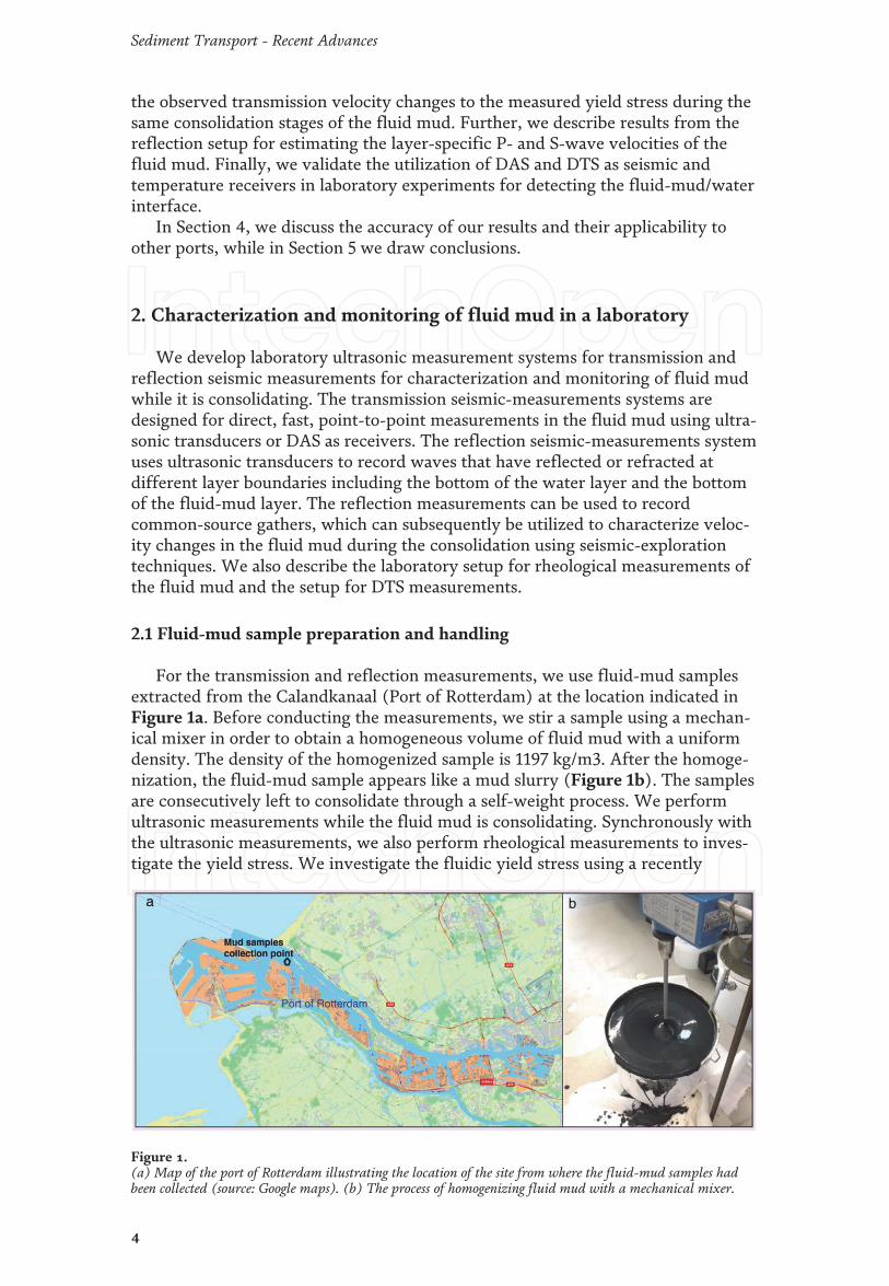
For the transmission and reflection measurements, we use fluid-mud samplesextracted from the Calandkanaal (Port of Rotterdam) at the location indicated inFigure 1a. Before conducting the measurements, we stir a sample using a mechan-ical mixer in order to obtain a homogeneous volume of fluid mud with a uniformdensity. The density of the homogenized sample is 1197 kg/m3. After the homoge-nization, the fluid-mud sample appears like a mud slurry (Figure 1b). The samplesare consecutively left to consolidate through a self-weight process. We performultrasonic measurements while the fluid mud is consolidating. Synchronously withthe ultrasonic measurements, we also perform rheological measurements to inves-tigate the yield stress. We investigate the fluidic yield stress using a recently

Figure 1.(a) Map of the port of Rotterdam illustrating the location of the site from where the fluid-mud samples hadbeen collected (source: Google maps). (b) The process of homogenizing fluid mud with a mechanical mixer.

4


developed protocol for the fluid mud [39, 40]. We use a HAAKE MARS I rheometer(Thermo Scientific) with two measuring geometries (Couette and vane) and applystress ramp-up tests to measure the yield stress. The stress ramp-up tests areperformed using a stress increase from 0 to 500 Pa at a rate of 1 Pa/s, until the shearrate reaches 300 s�1, under a stress-control mode.

2.2 Transmission seismic measurements with transducer receivers

The transmission seismic laboratory setup is equipped with two pairs of piezo-electric ultrasonic transducers (Figure 2b and c). Each pair consists of a source andreceiver transducer, with one of the pairs using P-wave transducers and the otherpair – S-wave transducers. The direct transmission measurement represents a point-to-point measurement with both transducer pairs placed along the horizontaldirection. Because of this source-receiver geometry, the estimated velocities of theP- and S- waves correspond to transmissions along horizontal layers inside the fluidmud, if such layers are developed.

As shown in Figure 2a, the laboratory setup includes a fluid-mud tank, a signal-control part, and the two pairs of ultrasound transducers. The signal-control part inturn consists of a source-control part and a receiver-control part. In the source-control part, a function generator produces a desired signal, which signal is subse-quently passed to a power amplifier to be finally passed to the source transducer,which sends it through the fluid mud. The fluid-mud tank is a plastic box that has

Figure 2.(a) Sketch of the transmission seismic laboratory setup with the fluid-mud box viewed from above andshowing the horizontal arrangement of the two transducer pairs. (b) Side view of the fluid-mud box showingthe vertical alignment of the ultrasonic transducers. (c) Photo of the fluid-mud box showing also the two sourcetransducers.

5


opening for the installation of the transducer end-caps. The receiver-control part ofthe setup consists of the receiver transducers, attached to the fluid-mud tank usingend-caps, an oscilloscope for digitalization and displaying, and a computer,connected to the oscilloscope, to record the sensed signals. The generated sourcesignal is also visualized on the oscilloscope for quality control.

For the transmission measurements, we use as a source signal a gated sine-wavepulse with a center frequency of 1 MHz. A measurement is performed using a pulse-time delay. To increase the signal-to-noise ratio, especially needed for the S-wavevelocity estimations, a measurement at each stage of consolidation consists of 1024repeated recordings summed together to obtain a final transmission recording. Thisis done for both the P- and S-wave pair.

For each stage of the measurements, the first step in estimating the propagationvelocities is to pick the first arrivals of the P- and S-waves. The second step is tocalculate the P- and S-wave velocities by dividing the travel distance of waves,which is the distance from the source to the receiver transducer within each pair(equal for both pairs), by the travel times estimated from the picked first arrivals.

2.3 Reflection seismic measurements with transducer receivers

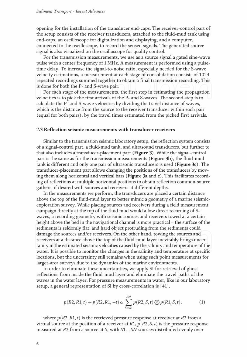
Similar to the transmission seismic laboratory setup, the reflection system consistsof a signal-control part, a fluid-mud tank, and ultrasound transducers, but further tothat also includes a transducer-placement part (Figure 3). While the signal-controlpart is the same as for the transmission measurements (Figure 3b), the fluid-mudtank is different and only one pair of ultrasonic transducers is used (Figure 3c). Thetransducer-placement part allows changing the positions of the transducers by mov-ing them along horizontal and vertical bars (Figure 3a and c). This facilitates record-ing of reflections at multiple horizontal positions to obtain reflection common-sourcegathers, if desired with sources and receivers at different depths.

In the measurements we perform, the transducers are placed a certain distanceabove the top of the fluid-mud layer to better mimic a geometry of a marine seismic-exploration survey. While placing sources and receivers during a field measurementcampaign directly at the top of the fluid mud would allow direct recording of S-waves, a recording geometry with seismic sources and receivers towed at a certainheight above the bed in the navigational channel is more practical – the surface of thesediments is seldomly flat, and hard object protruding from the sediments coulddamage the sources and/or receivers. On the other hand, towing the sources andreceivers at a distance above the top of the fluid-mud layer inevitably brings uncer-tainty in the estimated seismic velocities caused by the salinity and temperature of thewater. It is possible to monitor the changes in the salinity and temperature at specificlocations, but the uncertainty still remains when using such point measurements forlarger-area surveys due to the dynamics of the marine environments.

In order to eliminate these uncertainties, we apply SI for retrieval of ghostreflections from inside the fluid-mud layer and eliminate the travel-paths of thewaves in the water layer. For pressure measurements in water, like in our laboratorysetup, a general representation of SI by cross-correlation is [41].

p R2,R1, tð Þ þ p R2,R1,�tð Þ∝XSN

S¼S1

p R2, S, tð Þ⨂ p R1, S, tð Þ, (1)

where p R2,R1, tð Þ is the retrieved pressure response at receiver at R2 from avirtual source at the position of a receiver at R1, p R2, S, tð Þ is the pressure responsemeasured at R2 from a source at S, with S1… SN sources distributed evenly over

6


surface that effectively surrounds the two receivers, �t indicates time reversal(acausal time), and ⨂ indicates correlation. As mentioned above, when theassumptions for this simplified representation are not met [14], e.g. as in a seismicreflection survey when the sources are only at the surface and thus do not surroundthe receivers, ghost reflections are retrieved [17, 18], and we can write

p R2,R1, tð Þ þ p R2,R1,�tð Þ þ ghosts∝XSK2

S¼SK1

p R2, S, tð Þ⨂ p R1, S, tð Þ, (2)

Figure 3.Reflection seismic-measurements system. (a) Cartoon of the fluid-mud tank with the transducer-placement partand the signal-control part (identical to the one in the transmission measurements). Red star indicates the sourceand black probe indicates the receiver. The transducer-placement part allows vertical (blue arrows) andhorizontal (white arrows) displacement of the source and receiver. (b) Photo of the signal-control part. (c) Photoof the fluid-mud tank and the transducer-placement part with a source and receiver ultrasonic transducers.

7


where ghosts represents retrieved non-physical arrivals, including ghost reflec-tions, and SK1 and SK2 now indicate that the summation is only over sources on alimited surface. For practical purposes, in our laboratory setup we choose to haveonly two source positions and multiple receiver positions. Using source-receiverreciprocity, we can thus rewrite relation (2) as

p S2, S1, tð Þ þ p S2, S1,�tð Þ þ ghosts∝XRK2

R¼RK1

p S2,R, tð Þ⨂ p S1,R, tð Þ, (3)

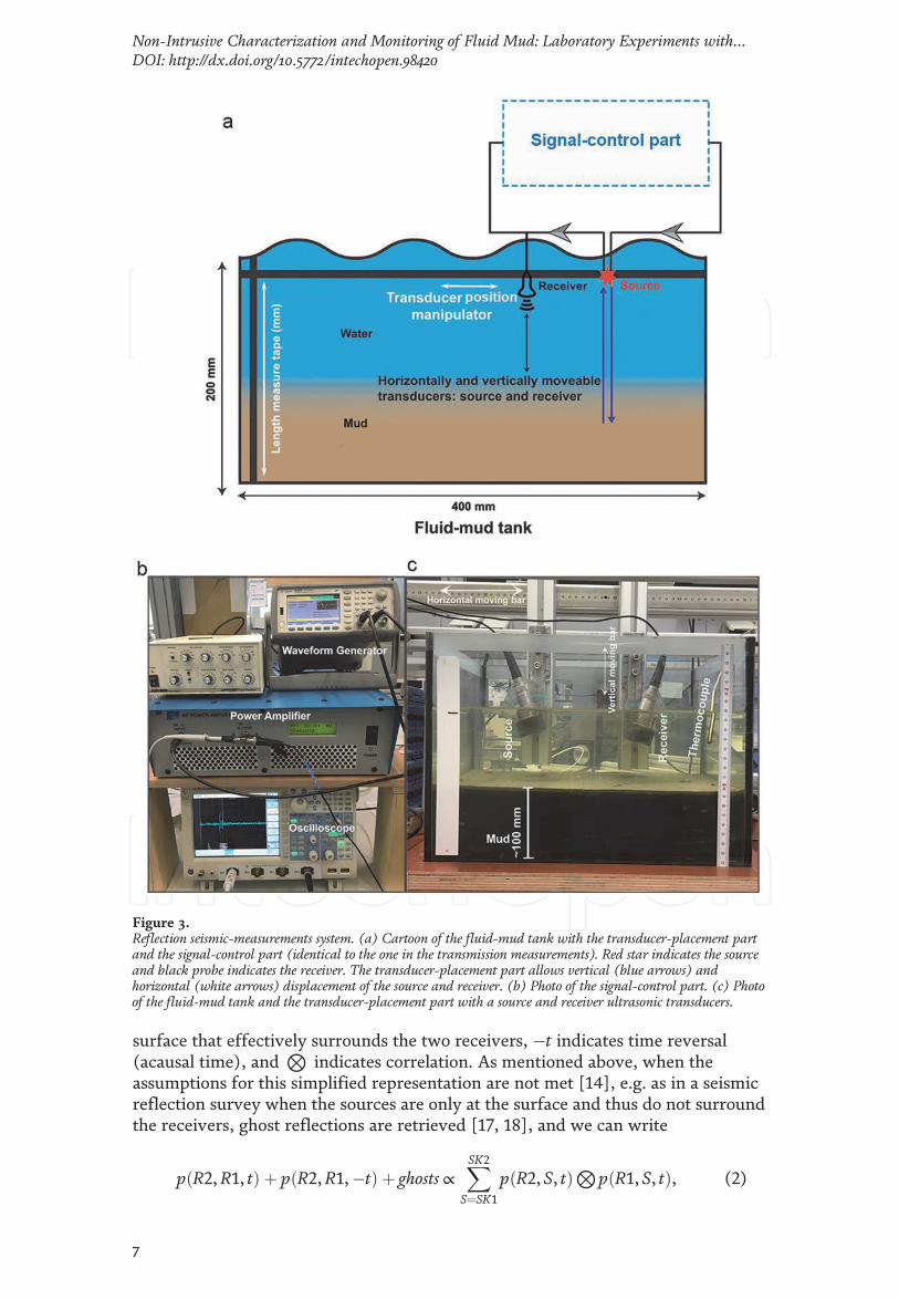
where the summation is now over receiver positions and we retrieve a pressurerecording at a virtual receiver at the position of source S2 from a sourse at S1. Thus,to apply SI, we use two common-source gathers (CSGs). The two source positions(labeled Source 1 or S1 and Source 2 or S2 in Figures 4 and 5, respectively) at thesame height and distanced in the horizontal direction 50 mm from each other. Werecord the reflected signal at a receiver, labeled Receiver 1 (R1) in Figure 4, alignedwith the two source positions and distanced 100 mm from S1 (and thus 50 mmfrom S2). Following the nomenclature in [17], the source and virtual receiverredatumed by SI to the top of the fluid-mud layer during the ghost-reflectionretrieval are referred to as ghost source and ghost receiver, respectively. Assuming afavorable geometry, to explain the retrieval of a ghost reflection inside the fluid-mud layer, the travel-path of the reflection from the fluid-mud bottom, i.e., thetravel-path starting from S1, transmitted at the water/mud interface, reflected bythe fluid-mud bottom, transmitted at the mud/water interface, and then arriving atR1 is labeled 1–2–3-4 in Figure 4. The travel-path of the reflection from the water/mud interface, starting from S2 and arriving at R1, is labeled 10-40. Cross-correlationof the recorded reflections at R1 from S1 and S2 will effectively result in removal ofthe common travel-paths in 1–2–3-4 and 10-40. Thus, the parallel travel-paths 1 and10 and the coinciding travel-paths 4 and 40 are eliminated, and only the travel-path2–3 is left over representing a ghost reflection only inside the fluid-mud layer from aghost source and ghost receiver placed directly at its top (Figure 4). In reality, theexact receiver position ensuring that travel-paths 1 = 10 and 4 = 40 is unknown.Because of that, recordings at multiple receiver positions from both sources arerequired, i.e., two CSGs. To obtain such gathers, we displace the receiver fromposition R1 to the right along the horizontal bar by 5 mm multiple times and record

Figure 4.Illustration of the geometry needed for retrieval of ghost reflections from inside the fluid-mud layer. See text forexplanation of the symbols.

8


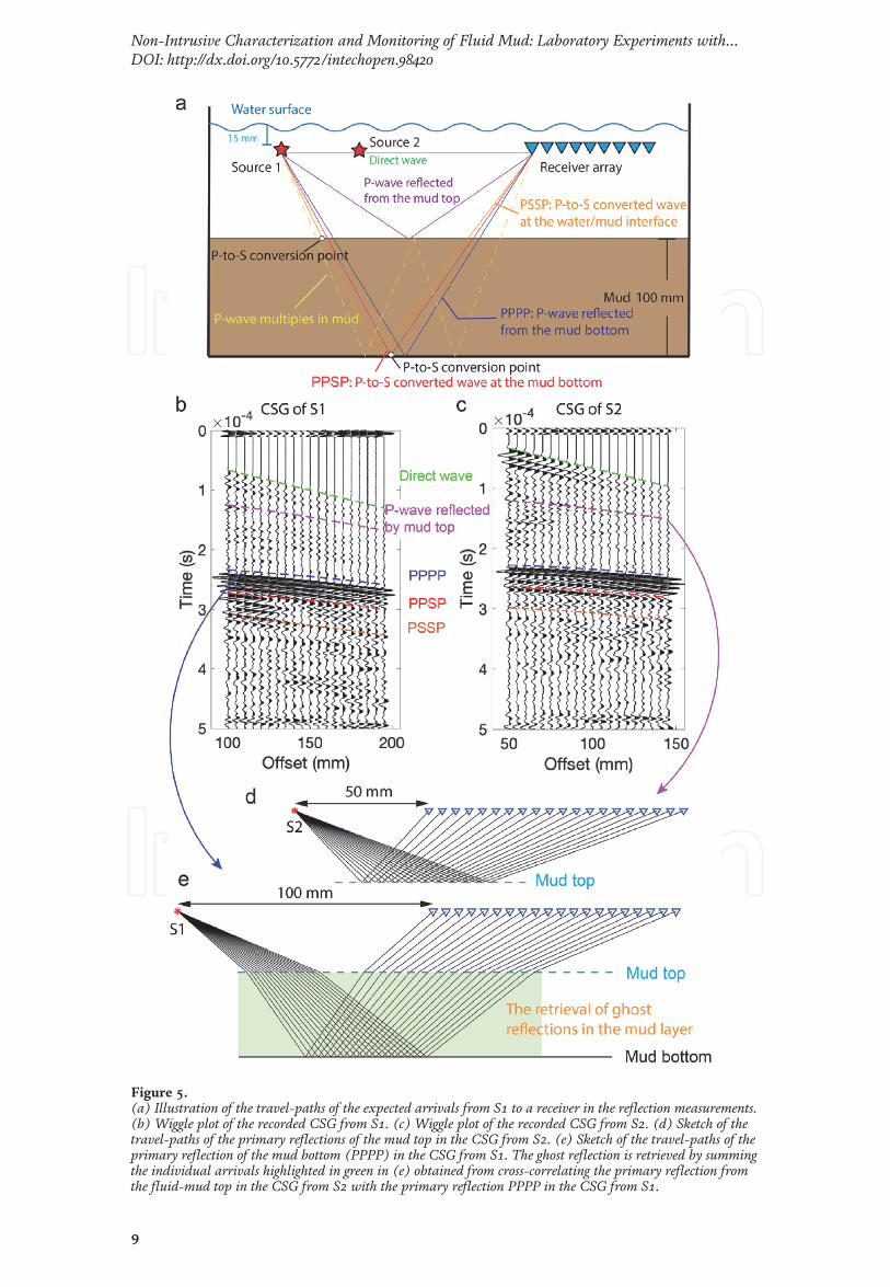
Figure 5.(a) Illustration of the travel-paths of the expected arrivals from S1 to a receiver in the reflection measurements.(b) Wiggle plot of the recorded CSG from S1. (c) Wiggle plot of the recorded CSG from S2. (d) Sketch of thetravel-paths of the primary reflections of the mud top in the CSG from S2. (e) Sketch of the travel-paths of theprimary reflection of the mud bottom (PPPP) in the CSG from S1. The ghost reflection is retrieved by summingthe individual arrivals highlighted in green in (e) obtained from cross-correlating the primary reflection fromthe fluid-mud top in the CSG from S2 with the primary reflection PPPP in the CSG from S1.

9


for the same source at each receiver position. In this case, we record at 20 positions.That is, the CSGs for S1 and S2 consist of 20 traces each.

The source signal we use is similar to the one for the transmission measurementsbut with a center frequency of 100 kHz.

Also with these measurements, to increase the signal-to-noise ratio of therecorded signals, a measurement at each receiver position from each source isrepeated 1024 times and the 1024 measurements are summed together to obtain afinal trace for that source and receiver positions.

Using the travel-path sketches in Figure 5a, we explain several arrivals of inter-est in the CSGs. Figure 5b and c present wiggle plots of the recorded CSGs from S1and S2, respectively. We calculate expected arrival times based on the source/receiver offsets and the thicknesses of the water and fluid-mud layers, each ofwhich we can directly measure. For propagation through the water layer, we useP-wave velocity of 1500 m/s. For the waves propagating through the fluid mud, weuse values estimated from the transmission measurements – 1570 m/s for theP-wave velocity and 958 m/s for the S-wave velocity. The calculated reference timesare illustrated by dashed lines superimposed on the CSGs to assist in interpretationof the arrivals. In Figure 5b and c, the reflection arrivals of interest in this study arethe primary reflection from the fluid-mud top (magenta) and the three primaryreflections from the fluid-mud bottom that are labeled as PPPP (blue), PPSP (red),and PSSP (orange). The S-waves in the experiment appear as waves converted fromP to S at the top or the bottom of the fluid-mud layer. For example, the P-to-Sconverted wave in PPSP is generated when the P-wave impinging on the fluid-mudbottom is reflected as an S-wave; the P-to-S converted wave in PSSP is generatedwhen the P-wave impinging on the fluid-mud top in transmitted to the fluid mud asan S-wave (Figure 5a) and continues to propagate as an S-wave until reaching thefluid-mud top again.

To retrieve ghost reflections, one can use relation (3) and correlate the CSGs.Such an approach could result in other retrieved arrivals interfering with thedesired ghost reflections. To avoid that, we follow [17] and correlate only specificarrivals. To retrieve a P-wave ghost reflection from inside the fluid mud, we cross-correlate the primary reflection from the fluid-mud top in the CSG from S2(Figure 5d) with the primary reflection PPPP in the CSG from S1 (Figure 5e). In asimilar way, the P-to-S converted ghost reflection and S-wave ghost reflection areretrieved using the reflections PPSP and PSSP in the CSG from S1, respectively.

2.4 Transmission seismic measurements using DAS and measurementswith DTS

We use a standard single-mode communication fiber for both the DAS and DTSmeasurements. This means that we can combine the two methods and compare thedifference in their performance With DAS, such fibers can act as seismic receiversthat measure the dynamics of a strain field acting on a fiber [42]. With DTS, suchfibers can act as strain and temperature sensors (and thus also labeled DT(S)S),which measure the static strain and temperature along the fiber [43].

To verify that these fibers can serve as receivers for fluid-mud level detectionand characterization, we conduct seismic and temperature laboratory experimentsusing commercially available interrogators. These interrogators are the iDAS fromSilixa and DITEST STA-R from Omnisens for measuring the acoustic impedanceand temperature, respectively. For a more detailed explanation of the iDAS system,the reader is referred to [42].

Our fiber is coiled around a PVC pipe with a diameter of 0.125 m, which allowsus to use more fiber and, hence, have more measuring points than when using a

10


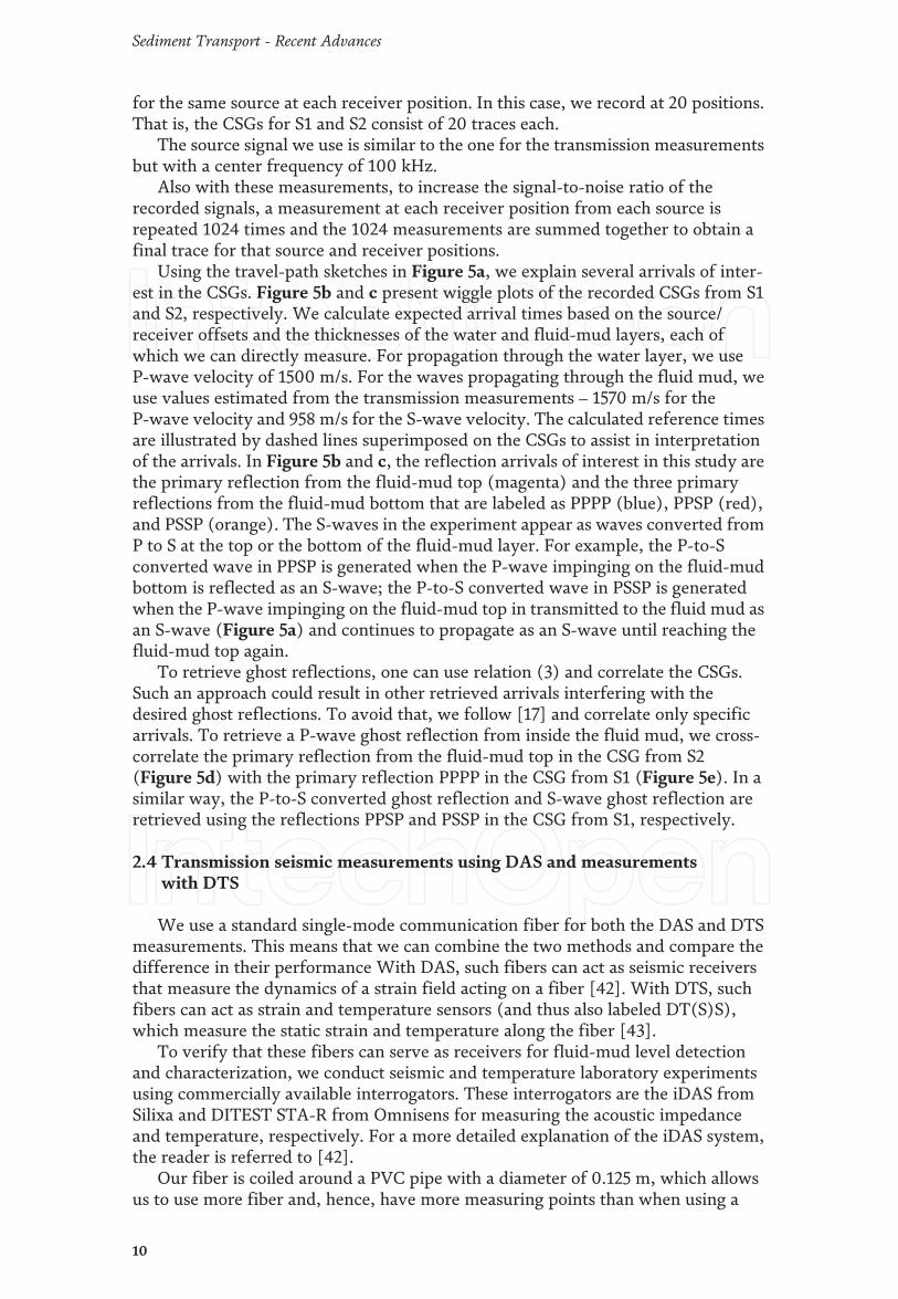
straight fiber. In addition, the coining increases the vertical resolution bycompressing the gauge length of 10 m of the cable (the length over which the back-scattered signal is averaged to increase the signal-to-noise ratio of the detecteddynamic deformation) only over a few vertical centimeters. Due to the coiling, wealso change the directional sensitivity [44], making the cable more sensitive tohorizontal waves, with respect to the column. The PVC pipe with the fiber coiled onit is placed inside a transparent column. We first perform experiments with twotypes of synthetic clay, namely kaolinite and bentonite, and subsequently with twotypes of fluid mud – one from the Port of Rotterdam, which is the same sample mudas described above, and the other from the Port of Hamburg. For the experimentswith the synthetic clays, we fill the lowest part of the column, without coiled opticalfiber, with sand. Above the sand, we put one of the clays, and then we fill theremainder with water. For the fluid-mud experiments, we instrument also thelowest part of the column with fiber and start filling the column with one of thefluid muds starting already at the bottom, while we again fill the remainder of thecolumn with water. A schematic overview and pictures of the setup are shown inFigure 6. Note that for the measurements with kaolinite and bentonite, we have0.5 m in depth, which is 123 m in fiber length, acting as sensors. For the measure-ments in the muds, we added 0.2 m in depth, giving us a total of 171 m of fiberlength, acting as sensors. For both setups, we have 10 m of fiber outside of ourcolumn to use as a reference.

With DAS, we try to capture the water/mud interface and measure the shearstrength build-up. We test various sources for these purposes. Our sources include asmall transducer with a center frequency of 500 kHz, a larger transducer with acenter frequency of 200 kHz (Figure 6b and c) and a common duo echo-sounderwith a center frequency of 38 kHz and 200 kHz, which is also used by marinevessels to measure depth. We connect these sources to the same source-side signal-control part as described above. We use a frequency range from 25 kHz to 45 kHz,since preliminary results indicated that this range should give the best results. Thesampling frequency of the DAS system is set at the maximum of the system, whichis 100 kHz.

For the DTS measurements, we use two standard heating rods, which we place5 cm away from the fiber, to heat the column and measure the difference withrespect to time along the column. This we only do for the kaolinite sample, since avery similar result is expected for the other clay and two mud samples.

Figure 6.(a) Schematic overview of the setup for DAS and DTS measurements. A photo of the column with the opticalfiber wound around the PVC pipe when using mud from the (b) port of Rotterdam and (c) port of Hamburg.

11


3. Results

We describe the results of the ultrasonic transmission measurements with ultra-sonic transducers and correlate them to the results from the rheological measure-ments. We further report the results from the reflection measurements and howthey were used to retrieve ghost reflections. We then show the results from the DASand DTS measurements.

3.1 P- and S-waves velocities in the fluid mud from transmission measurementswith ultrasonic transducers

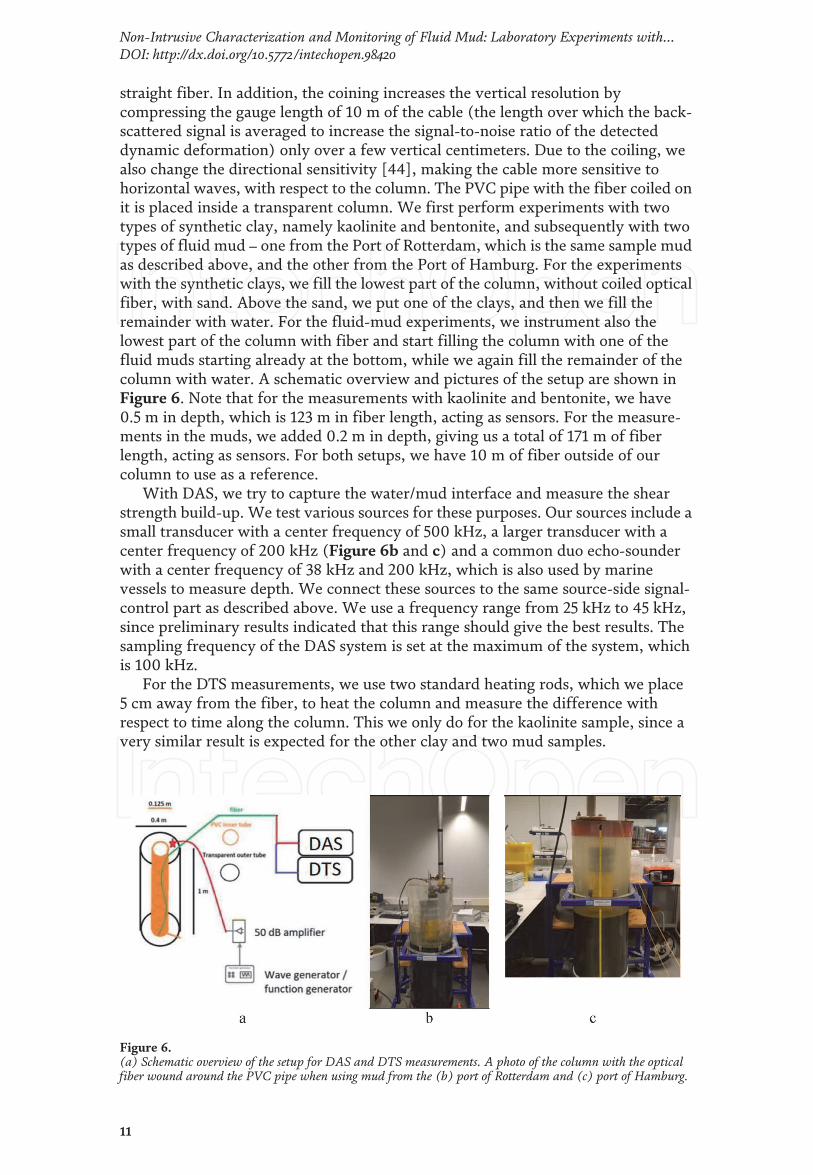
We examine the first arrivals of transmitted P- and S-waves and estimate theirvelocity variations during the consolidation of the fluid mud. We do not observe adetectable change in the P-wave velocity – the P-wave first arrivals appear to beconstant throughout the consolidation process (Figure 7a). This finding agrees withprevious results reporting that the S-wave velocity is more sensitive to changes inlithology and mechanical properties than the P-wave velocity [45]. The traveltimeof the direct arrivals of the P-wave is 0.074 ms (Figure 7a), and thus thecorresponding velocity is 1570 m/s. By examining the change in arrival time of the

Figure 7.(a) Transmission recordings of the direct P- and S-wave arrivals as a function of consolidation time. (b)Estimated S-wave velocity as a function of the consolidation time.

12


first S-wave arrival (Figure 7a), we find that the S-wave traveltime decreases withconsolidation time, indicating that the S-wave velocity increases with the consoli-dation progress (Figure 7b).

We can see from Figure 7, that during the first three days the S-wave velocity isnearly stable exhibiting very little fluctuations. Starting from Day 3, the S-wavevelocity shows a strong increase from 959 to 995 m/s during the next two days. Inthe second week, the S-wave velocity only experiences a small increase and even-tually reaches 998 m/s. By comparing the velocity variations of the P-wave and S-waves, we can summarize that the relative increase in the S-wave velocity is muchstronger than in P-wave velocities, validating the statement that the S-waves aremuch more sensitive to the consolidation of the fluid mud than the P-waves. Thisfinding agrees with a previous in-situ seismic exploration results using pulse-transmission techniques [45].

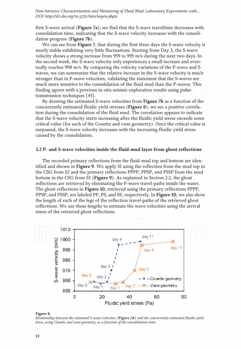
By drawing the estimated S-wave velocities from Figure 7b as a function of theconcurrently estimated fluidic yield stresses (Figure 8), we see a positive correla-tion during the consolidation of the fluid mud. The correlation appears to indicatethat the S-wave velocity starts increasing after the fluidic yield stress exceeds somecritical value (for each of the Couette and vane geometry). Once the critical value issurpassed, the S-wave velocity increases with the increasing fluidic yield stresscaused by the consolidation.

3.2 P- and S-wave velocities inside the fluid-mud layer from ghost reflections

The recorded primary reflections from the fluid-mud top and bottom are iden-tified and shown in Figure 9. We apply SI using the reflection from the mud top inthe CSG from S2 and the primary reflections PPPP, PPSP, and PSSP from the mudbottom in the CSG from S1 (Figure 9). As explained in Section 2.2, the ghostreflections are retrieved by eliminating the P-wave travel-paths inside the water.The ghost reflections in Figure 10, retrieved using the primary reflections PPPP,PPSP, and PSSP, are labeled PP, PS, and SS, respectively. In Figure 10, we also showthe length of each of the legs of the reflection travel-paths of the retrieved ghostreflections. We use these lengths to estimate the wave velocities using the arrivaltimes of the retrieved ghost reflections.

Figure 8.Relationship between the estimated S-wave velocities (Figure 7b) and the concurrently estimated fluidic yieldstress, using Couette and vane geometry, as a function of the consolidation time.

13


As explained, the retrieved result is obtained by stacking the correlated traces.When the receiver array is sufficiently long, the stacking would have resulted in theretrieved ghost reflections only, with the contribution to the retrieved signalcoming from summation inside the so-called stationary-phase region [46], i.e., theregion where a curve appears nearly horizontal. In Figures 11a–13a, we indicate thestationary-phase regions with green dashed rectangles. Because our receiver array isof a limited length and is further only on one side of the sources, summation of alltraces produces more or less erroneous results (Figures 11b–13b). Because of this,to retrieve the ghost reflections we use for the summation only traces in thestationary-phase region (Figures 11c–13c). We then pick from those results thetwo-way traveltimes to estimate the velocities inside the fluid-mud layer.

Figure 9.Identified primary reflections in the common-source gather from (a) source 1 and (b) source 2. We applyseismic interferometry (SI) by correlating (the ⊗ symbol) the reflection from the mud top with each of the threeidentified reflections from the mud bottom followed by summation over the receivers (Eq. 3).

Figure 10.The travel distances of the travel-paths of the ghost reflections PP, SS, and PS when the fluid-mud thickness is86 mm, which is the thickness on day 11 of the consolidation.

14


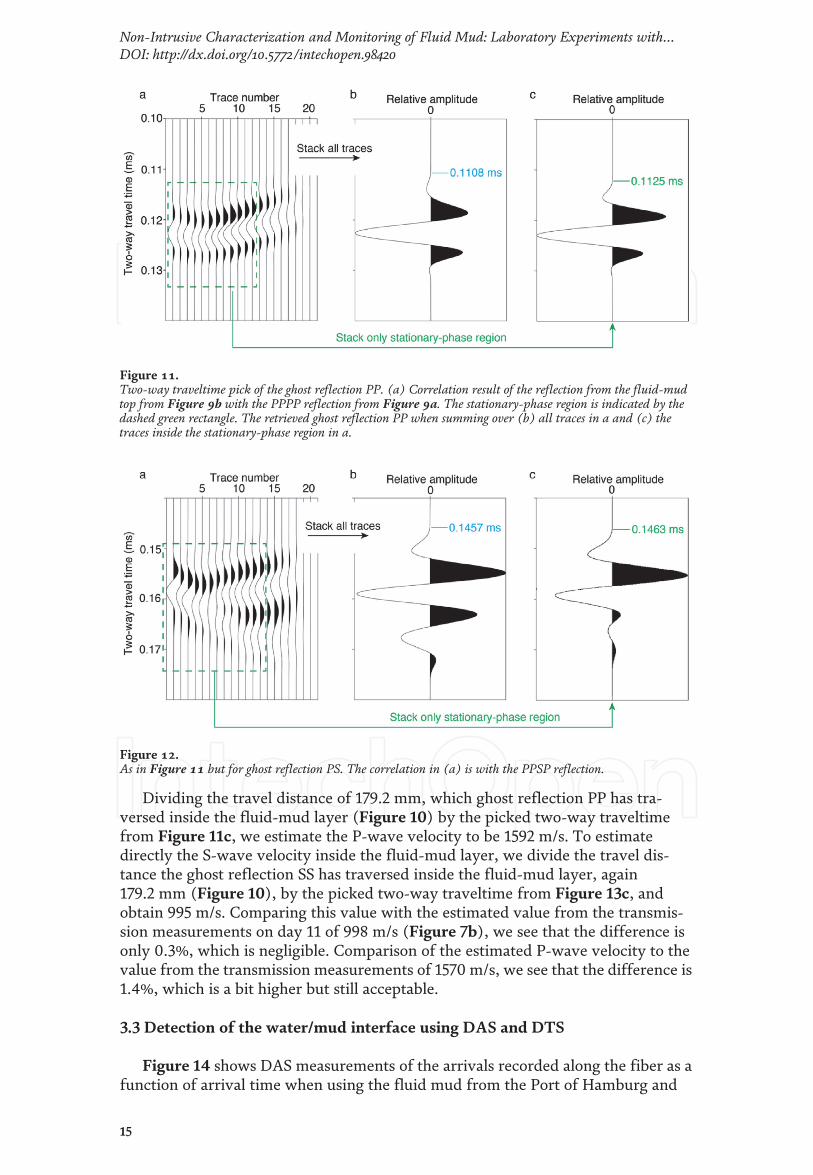
Dividing the travel distance of 179.2 mm, which ghost reflection PP has tra-versed inside the fluid-mud layer (Figure 10) by the picked two-way traveltimefrom Figure 11c, we estimate the P-wave velocity to be 1592 m/s. To estimatedirectly the S-wave velocity inside the fluid-mud layer, we divide the travel dis-tance the ghost reflection SS has traversed inside the fluid-mud layer, again179.2 mm (Figure 10), by the picked two-way traveltime from Figure 13c, andobtain 995 m/s. Comparing this value with the estimated value from the transmis-sion measurements on day 11 of 998 m/s (Figure 7b), we see that the difference isonly 0.3%, which is negligible. Comparison of the estimated P-wave velocity to thevalue from the transmission measurements of 1570 m/s, we see that the difference is1.4%, which is a bit higher but still acceptable.

3.3 Detection of the water/mud interface using DAS and DTS

Figure 14 shows DAS measurements of the arrivals recorded along the fiber as afunction of arrival time when using the fluid mud from the Port of Hamburg and

Figure 11.Two-way traveltime pick of the ghost reflection PP. (a) Correlation result of the reflection from the fluid-mudtop from Figure 9b with the PPPP reflection from Figure 9a. The stationary-phase region is indicated by thedashed green rectangle. The retrieved ghost reflection PP when summing over (b) all traces in a and (c) thetraces inside the stationary-phase region in a.

Figure 12.As in Figure 11 but for ghost reflection PS. The correlation in (a) is with the PPSP reflection.

15


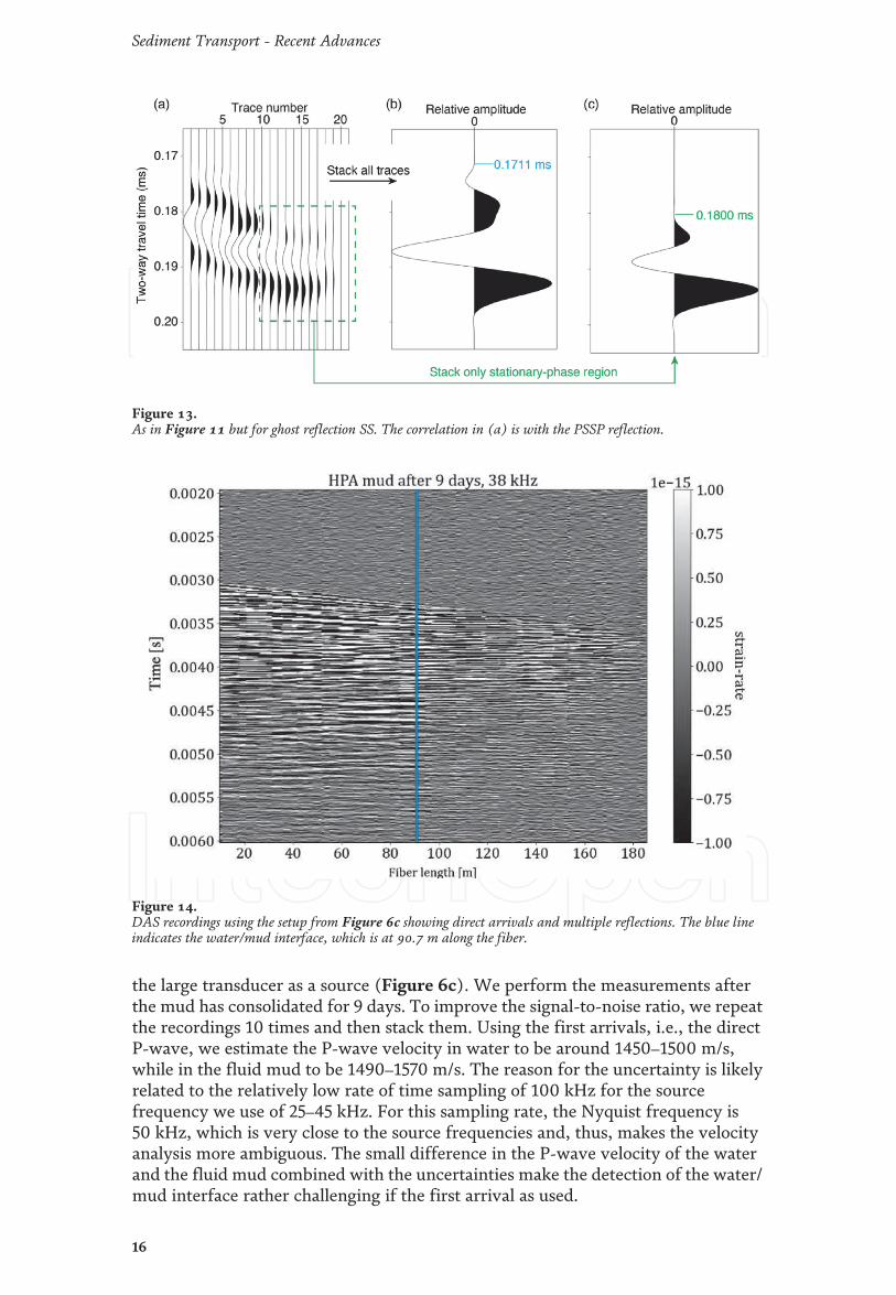
the large transducer as a source (Figure 6c). We perform the measurements afterthe mud has consolidated for 9 days. To improve the signal-to-noise ratio, we repeatthe recordings 10 times and then stack them. Using the first arrivals, i.e., the directP-wave, we estimate the P-wave velocity in water to be around 1450–1500 m/s,while in the fluid mud to be 1490–1570 m/s. The reason for the uncertainty is likelyrelated to the relatively low rate of time sampling of 100 kHz for the sourcefrequency we use of 25–45 kHz. For this sampling rate, the Nyquist frequency is50 kHz, which is very close to the source frequencies and, thus, makes the velocityanalysis more ambiguous. The small difference in the P-wave velocity of the waterand the fluid mud combined with the uncertainties make the detection of the water/mud interface rather challenging if the first arrival as used.

Figure 13.As in Figure 11 but for ghost reflection SS. The correlation in (a) is with the PSSP reflection.

Figure 14.DAS recordings using the setup from Figure 6c showing direct arrivals and multiple reflections. The blue lineindicates the water/mud interface, which is at 90.7 m along the fiber.

16


The recordings in Figure 14 show that a more accurate and robust criterion todetect the water/mud interface is to look at the multiple reflections and theiramplitude attenuation. Looking at the figure, we can see that later arrivals appear tofaint, i.e., are more attenuated after the water/mud interface, with the latter indi-cated by the blue line. Taking a closer look at the multiple reflections, we see thatthese later arrivals have completely fainted after 93.7 m fiber length, with thewater/mud interface at 90.7 m fiber length. This difference of 3 m of fiber might berelated to the gauge length of the fiber, i.e., the length over which the DAS systemaverages the observations, which in our case is 10 m. Another reason could be theuncertainty in the exact position of the fiber.

The measurements with the fluid mud from the Port of Rotterdam and the twoclays show similar results.

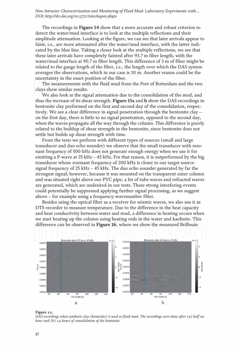
We also look at the signal attenuation due to the consolidation of the mud, andthus the increase of its shear strength. Figure 15a and b show the DAS recordings inbentonite clay performed on the first and second day of the consolidation, respec-tively. We see a clear difference in signal penetration through the bentonite clay –

on the first day, there is little to no signal penetration, opposed to the second day,when the waves propagate all the way through the column. This difference is purelyrelated to the buildup of shear strength in the bentonite, since bentonite does notsettle but builds up shear strength with time.

From the tests we perform with different types of sources (small and largetransducer and duo echo sounder) we observe that the small transducer with reso-nant frequency of 500 kHz does not generate enough energy when we use it foremitting a P-wave at 25 kHz – 45 kHz. For that reason, it is outperformed by the bigtransducer whose resonant frequency of 200 kHz is closer to our target source-signal frequency of 25 kHz – 45 kHz. The duo echo sounder generated by far thestrongest signal; however, because it was mounted on the transparent outer columnand was situated right above our PVC pipe, a lot of tube waves and refracted wavesare generated, which are undesired in our tests. These strong interfering eventscould potentially be suppressed applying further signal processing, as we suggestabove – for example using a frequency-wavenumber filter.

Besides using the optical fiber as a receiver for seismic waves, we also use it asDTS recorder to measure temperature. Due to the difference in the heat capacityand heat conductivity between water and mud, a difference in heating occurs whenwe start heating up the column using heating rods in the water and kaolinite. Thisdifference can be observed in Figure 16, where we show the measured Brillouin

Figure 15.DAS recordings when synthetic clay (bentonite) is used as fluid mud. The recordings were done after (a) half anhour and (b) 24 hours of consolidation of the bentonite.

17


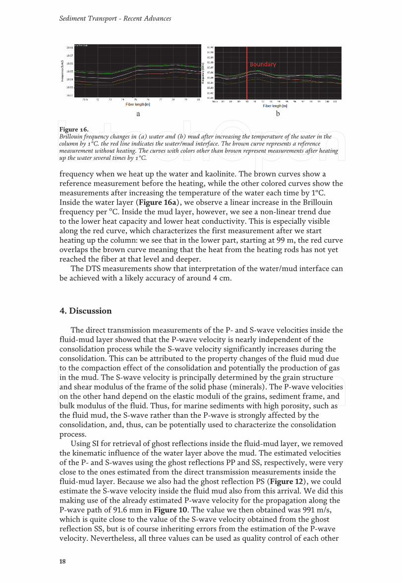
frequency when we heat up the water and kaolinite. The brown curves show areference measurement before the heating, while the other colored curves show themeasurements after increasing the temperature of the water each time by 1°C.Inside the water layer (Figure 16a), we observe a linear increase in the Brillouinfrequency per oC. Inside the mud layer, however, we see a non-linear trend dueto the lower heat capacity and lower heat conductivity. This is especially visiblealong the red curve, which characterizes the first measurement after we startheating up the column: we see that in the lower part, starting at 99 m, the red curveoverlaps the brown curve meaning that the heat from the heating rods has not yetreached the fiber at that level and deeper.

The DTS measurements show that interpretation of the water/mud interface canbe achieved with a likely accuracy of around 4 cm.

4. Discussion

The direct transmission measurements of the P- and S-wave velocities inside thefluid-mud layer showed that the P-wave velocity is nearly independent of theconsolidation process while the S-wave velocity significantly increases during theconsolidation. This can be attributed to the property changes of the fluid mud dueto the compaction effect of the consolidation and potentially the production of gasin the mud. The S-wave velocity is principally determined by the grain structureand shear modulus of the frame of the solid phase (minerals). The P-wave velocitieson the other hand depend on the elastic moduli of the grains, sediment frame, andbulk modulus of the fluid. Thus, for marine sediments with high porosity, such asthe fluid mud, the S-wave rather than the P-wave is strongly affected by theconsolidation, and, thus, can be potentially used to characterize the consolidationprocess.

Using SI for retrieval of ghost reflections inside the fluid-mud layer, we removedthe kinematic influence of the water layer above the mud. The estimated velocitiesof the P- and S-waves using the ghost reflections PP and SS, respectively, were veryclose to the ones estimated from the direct transmission measurements inside thefluid-mud layer. Because we also had the ghost reflection PS (Figure 12), we couldestimate the S-wave velocity inside the fluid mud also from this arrival. We did thismaking use of the already estimated P-wave velocity for the propagation along theP-wave path of 91.6 mm in Figure 10. The value we then obtained was 991 m/s,which is quite close to the value of the S-wave velocity obtained from the ghostreflection SS, but is of course inheriting errors from the estimation of the P-wavevelocity. Nevertheless, all three values can be used as quality control of each other

Figure 16.Brillouin frequency changes in (a) water and (b) mud after increasing the temperature of the water in thecolumn by 1°C. the red line indicates the water/mud interface. The brown curve represents a referencemeasurement without heating. The curves with colors other than brown represent measurements after heatingup the water several times by 1°C.

18


or as substitutes when one of the three ghost reflections cannot be reliably retrieveddue to, for example, interference from other arrivals.

Observing the multiple reflections in the DAS recordings, we estimated an errorof 3 m along the coiled fiber in detecting the depth of the water/mud interface.Since we coiled the fiber around a PVC pipe with a diameter of 0.125 m and becausethe fiber’s thickness is 1.6 mm, the 3-meter error of fiber length translates to 1.2 cmof vertical error in the depth of the water/mud interface. With such an error, to thebest of our knowledge, our approach is the most accurate non-intrusive method fordetermining the depth of the water/mud interface. Note that to achieve this accu-rate result, the only processing we applied was to increase the signal-to-noise ratioby the summation of the 10 separate recordings. More signal processing couldfurther improve the determination of the water/mud interface. We expect that asimilar high accuracy is achievable in the field as well since the upper end of theoptical fiber is placed at the very bottom of the water layer, which limits errorscaused by differences in, for instance, the water temperature.

The direct transmission measurements with DAS, on the other hand, allowedestimation of the P-wave velocity in the fluid mud in the range 1490–1570 m/s.Comparing these values to the value of 1570 m/s from the direct transmissionmeasurements horizontally inside the fluid mud means an uncertainty of about5.1%, which is not negligible. This confirms the difficulty when using a source in thewater and receivers in the fluid mud, and clearly underlines the advantage of usingSI with ghost reflections from reflection measurements. Thus, we argue thatanother very useful application of DAS could be with direct transmission measure-ments inside the fluid-mud layer, and thus also for transmission tomographybetween a vertical array of sources inside the mud and a vertical DAS pole withcoiled fiber.

For our laboratory measurements, we used fluid-mud samples from the Port ofRotterdam and the Port of Hamburg. Nevertheless, our results and conclusions canbe generalized to fluid-mud samples from other ports. Because the estimated P- andS-wave velocities using the ghost reflections do not depend kinematically on thewater layer, this technique could easily be applied to any port or waterway. Ofcourse, the P- and S-wave velocities of the fluid mud will differ from place to place,so those will need to be estimated for each place, for example for correlation withthe yield stress. The DAS and DTS techniques for estimating the water/mudboundary can likewise be used at any other port or waterway, as they depend onlyon the strong contrast in the observed parameters between the layer and fluid-mudlayer.

5. Conclusions

We presented recent results for non-intrusive characterization and monitoringof fluid mud in ports and waterways using ultrasonic measurements in transmissionand reflection geometry, including measurements with Distributed Acoustic Sens-ing (DAS), and using temperature measurements with Distributed TemperatureSensing (DTS). We performed the measurements in a laboratory on samples fromthe Port of Rotterdam, Port of Hamburg, and two synthetic clays.

Using ultrasonic transmission measurements with transducers directly insidefluid mud, we investigated the changes in the velocities of longitudinal (P-) andtransverse (S-) waves and their possible relation to the yield stress during theconsolidation. We observed no detectable change of the P-wave velocities duringthe consolidation of the fluid mud. We observed that the S-wave velocitiesexhibited a relatively strong increase after the fluid mud settles for a certain amount

19


of time, in our study after 3 days. Comparing the estimated S-wave velocities to theconcurrently estimated fluidic yield stress, we showed a positive correlationbetween the two. Our findings verify that the S-wave velocities increase withincreasing yield stress caused by the fluid-mud consolidation and can thus bepotentially used for indirect in-situ assessment of the yield stress.

Using ultrasonic reflection measurements with transducers, we investigated thedirect estimation of the P- and S-wave velocities inside the fluid-mud layer. Thesource and receiver transducers were placed inside the water layer, but we showedthat the kinematic influence of the water layer can be completely eliminated byretrieval of non-physical (ghost) reflections inside the fluid mud by application ofseismic interferometry. Using the retrieved ghost reflections to estimate the layer-specific P- and S-waves velocities of the mud, we eliminated possible uncertaintydue to salinity and temperature gradients of the water, which affect the velocityestimates using the usual seismic-reflection processing techniques. We show thatthe reflection-estimated velocities differ from the transmission-calculated valuesonly by 1.4% and 0.3% for the P- and S-waves, respectively.

We also showed that DAS and DTS can be very effective in estimating the depthof the water/mud interface. We showed that a standard communication fiber issufficient to achieve an accuracy in the estimated depth of the water/mud interfaceof 1.2 cm. This accuracy, to the best of our knowledge, is higher than what isachievable with any the currently used non-intrusive methods. Furthermore, weshowed that the strength of the signal recorded with DAS is linked to changes in theshear strength of clays.

Acknowledgements

The research of X.M. is supported by the Division for Earth and Life Sciences(ALW) with financial aid from the Netherlands Organization for ScientificResearch (NWO) with grant no. ALWTW.2016.029. The research of M.B. issupported by the Port of Rotterdam, Hamburg Port Authority, Rijkswaterstaat andSmartPort. The project is carried out also within the framework of the MUDNETacademic network https://www.tudelft.nl/mudnet/.

Conflict of interest

The authors declare no conflict of interest.

20


Author details

Deyan Draganov1*, Xu Ma1, Menno Buisman1,2, Tjeerd Kiers1, Karel Heller1 andAlex Kirichek1,3

1 Faculty of Civil Engineering and Geosciences, Delft University of Technology,Delft, The Netherlands

2 Port of Rotterdam, Rotterdam, The Netherlands

3 Deltares, Delft, The Netherlands

*Address all correspondence to: [email protected]

© 2021 TheAuthor(s). Licensee IntechOpen. This chapter is distributed under the termsof theCreativeCommonsAttribution License (http://creativecommons.org/licenses/by/3.0),which permits unrestricted use, distribution, and reproduction in anymedium,provided the original work is properly cited.

21


References

[1]McAnally WH, Friedrichs C,Hamilton D, Hayter E, Shrestha P,Rodriguez H, Sheremet A, Teeter A,ASCE task committee on Managementof Fluid mud. Management of fluid mudin estuaries, bays, and lakes. I: Presentstate of understanding on character andbehavior. Journal of HydraulicEngineering. 2007 Jan;133(1):9-22.

[2]Harbour Approach Channels DesignGuidelines. In: Report of MarcomWorking Group. 2014. p. 49.

[3] Kirichek A, Chassagne C,Winterwerp H, Vellinga T. Hownavigable are fluid mud layers. Terra etAqua: International Journal on PublicWorks, Ports and WaterwaysDevelopments. 2018;151.

[4]Delefortrie G, Vantorre M, Eloot K.Modelling navigation in muddy areasthrough captive model tests. Journal ofmarine science and technology. 2005Dec 1;10(4):188-202.

[5] Vantorre M. Ship behaviour andcontrol in muddy areas: state of the art.InProceedings of the 3rd InternationalConference on Manoeuvring andControl of Marine Craft (MCMC'94),edited by GN Roberts and MMAPourzanjani, Southampton 1994 Sep(pp. 7-9).

[6] Claeys S, De Schutter J, Vantorre M,Van Hoestberghe T. Rheology as asurvey tool: We are not there yet. HydroInternational. 2011;15(3):14-19.

[7] Kirichek A, Rutgers R. Monitoring ofsettling and consolidation of mud afterwater injection dredging in theCalandkanaal. Terra et Aqua. 2020; 160:16-26

[8] Kirichek A, Shakeel A, Chassagne C.Using in situ density and strengthmeasurements for sedimentmaintenance in ports and waterways.

Journal of Soils and Sediments. 2020 Feb19:1-7.

[9]Hamilton EL, Bachman RT. Soundvelocity and related properties ofmarine sediments. The Journal of theAcoustical Society of America. 1982Dec;72(6):1891-1904.

[10] Schrottke K, Becker M,Bartholomä A, Flemming BW,Hebbeln D. Fluid mud dynamics in theWeser estuary turbidity zone tracked byhigh-resolution side-scan sonar andparametric sub-bottom profiler. Geo-Marine Letters. 2006 Sep 1;26(3):185-198.

[11]Gratiot N, Mory M, Auchere D. Anacoustic Doppler velocimeter (ADV) forthe characterisation of turbulence inconcentrated fluid mud. ContinentalShelf Research. 2000 Sep 10;20(12–13):1551-1567.

[12]Meissner R, Rabbel W, Theilen F.The relevance of shear waves forstructural subsurface investigations.InShear waves in marine sediments 1991(pp. 41-49). Springer, Dordrecht.

[13] Shapiro NM, Campillo M.Emergence of broadband Rayleighwaves from correlations of the ambientseismic noise. Geophysical ResearchLetters. 2004 Apr 16;31(7).

[14]Wapenaar K, Fokkema J. Green’sfunction representations for seismicinterferometry. Geophysics. 2006 Jul;71(4):SI33-SI46.

[15]Draganov D, Campman X,Thorbecke J, Verdel A, Wapenaar K.Reflection images from ambient seismicnoise. Geophysics. 2009 Sep;74(5):A63-A67.

[16]Draganov D, Ghose R, Ruigrok E,Thorbecke J, Wapenaar K. Seismic

22


interferometry, intrinsic losses and Q-estimation. Geophysical Prospecting.2010 Mar 26;58(3):361-373.

[17]Draganov D, Heller K, Ghose R.Monitoring CO2 storage using ghostreflections retrieved from seismicinterferometry. International Journal ofGreenhouse Gas Control. 2012 Nov 1;11:S35-S46.

[18] King S, Curtis A. Suppressingnonphysical reflections in Green’sfunction estimates using source-receiverinterferometrySuppressing nonphysicalreflections. Geophysics. 2012 Jan 1;77(1):Q15-Q25.

[19] Breitzke M. Acoustic and elasticcharacterization of marine sediments byanalysis, modeling, and inversion ofultrasonic P wave transmissionseismograms. Journal of GeophysicalResearch: Solid Earth. 2000 Sep 10;105(B9):21411-21430.

[20] Leurer KC. Compressional-andshear-wave velocities and attenuation indeep-sea sediment during laboratorycompaction. The Journal of theAcoustical Society of America. 2004Oct;116(4):2023-2030.

[21] Ballard MS, Lee KM, Muir TG.Laboratory P-and S-wavemeasurements of a reconstituted muddysediment with comparison to card-house theory. The Journal of theAcoustical Society of America. 2014Dec;136(6):2941-2946.

[22] Ballard MS, Lee KM. Examining theeffects of microstructure on geoacousticparameters in fine-grained sediments.The Journal of the Acoustical Society ofAmerica. 2016 Sep 8;140(3):1548-1557.

[23] Collins JA, Sutton GH, Ewing JI.Shear-wave velocity structure ofshallow-water sediments in the EastChina Sea. The Journal of the AcousticalSociety of America. 1996 Dec;100(6):3646-3654.

[24] Ajo-Franklin JB, Dou S, Lindsey NJ,Monga I, Tracy C, Robertson M,Rodriguez Tribaldos V, Ulrich C,Freifeld B, Daley T, Li X. Distributedacoustic sensing using dark fiber fornear-surface characterization andbroadband seismic event detection.Sientific Reports. 2019; 9:1328.

[25] Jousset P, Reinsch T, Ryberg T,Blanck H, Clarke A, Aghayev R,Hersir GP, Henninges J, Weber M,Krawczyk CM. Dynamic straindetermination using fibre-optic cablesallows imaging of seismological andstructural features. NatureCommunications. 2018; 9: 2509.

[26] Lindsey NJ, Martin ER, Dreger DS,Freifeld B, Cole S, James RS, Biondi BL,Ajo-Franklin JB. Fiber-optic networkobservations of earthquake Wavefields.Geophysical Research Letters. 2017 Dec16; 44(23):11792-11799.

[27]Wang HF, Zeng X, Miller DE,Fratta D, Feigl KL, Thurber CH,Mellors RJ. Ground motion response toan ML 4.3 earthquake using co-locateddistributed acoustic sensing andseismometer arrays. Geophysical JournalInternational. 2018 Jun;213(3):220-236.

[28] Yu C, Zhan Z, Lindsey NJ, Ajo-Franklin JB, Robertson M. The potentialof DAS in Teleseismic studies: Insightsfrom the goldstone experiment.Geophysical Research Letters. 2019 Feb16; 46(3):1320-1328.

[29]Daley TM, Miller DE, Dodds K,Cook P, Freifeld BM. Field testing ofmodular borehole monitoring withsimultaneous distributed acousticsensing and geophone vertical seismicprofiles at Citronelle, Alabama.Geophysical Prospecting. 2016; 64(5):1318-1334.

[30]Mateeva A, Lopez J, Potters H,Mestayer J, Cox B, Kiyashchenko D,Wills P, Grandi S, Hornman K,Kuvshinov B, Berlang W, Yang Z,

23


Detomo R. Distributed acoustic sensingfor reservoir monitoring with verticalseismic profiling. GeophysicalProspecting. 2014; 62(4):679–692.

[31] Zeng X, Lancelle C, Thurber C,Fratta D, Wang H, Lord N, Chalari A,Clarke A. Properties of noise cross-correlation functions obtained from adistributed acoustic sensing Array atGarner Valley, California. Bulletin of theSeismological Society of America. 2017Jan 31; 107(2):603-610.

[32] Ravet F, Rochat E, Niklès M.BOTDA-based DTS robustnessdemonstration for subsea structuremonitoring applications. Proc. SPIE9634, 24th International Conference onOptical Fibre Sensors. 2015 Sep 28;96345Z.

[33] Stork AL, Chalari A, Durucan S,Korre A, Nikolov S. Fibre-opticmonitoring for high-temperature carboncapture, utilization and storage (CCUS)projects at geothermal energy sites. FirstBreak. 2020 Oct; 38(10):61-67.

[34] Shao M, Qiao X, Zhao X, Zhang Y,Fu H. Liquid level sensor using fiberBragg grating assisted by multimodefiber core. IEEE Sensors Journal. 2016Jan 7;16(8):2374-2379.

[35] Xu W, Wang J, Zhao J, Zhang C,Shi J, Yang X, Yao J. Reflective liquidlevel sensor based on parallel connectionof cascaded FBG and SNCS structure.IEEE Sensors Journal. 2016 Nov 16;17(5):1347-1352.

[36] Yang C, Chen S, Yang G. Fiberoptical liquid level sensor undercryogenic environment. Sensors andActuators A: Physical. 2001 Oct 31;94(1–2):69-75.

[37]Wei M, McGuire JJ, Richardson E. Aslow slip event in the south CentralAlaska subduction zone and relatedseismicity anomaly. GeophysicalResearch Letters. 2012 Aug 16;39(15).

[38] Shizhuo Y, Ruffin PB, Francis TS.Fiber optic sensors. Talor & FrancisGroup. 2008;479.

[39] Shakeel A, Kirichek A, Chassagne C.Rheological analysis of mud from portof Hamburg, Germany. Journal of Soilsand Sediments. 2020; 1-10.

[40] Shakeel A, Kirichek A, Chassagne C.Yield stress measurements of mudsediments using different rheologicalmethods and geometries: An evidence oftwo-step yielding. Marine Geology.2020; 106247.

[41]Draganov D, Hunziker J, Heller K,Gutkowski K, Marte F, high-resolutionultrasonic imaging of artworks withseismic interferometry for theirconservation and restoration. Studies inConservation. 2018; 63(5):277-291.

[42] Lindsey NJ, Rademacher H,Ajo-Franklin JB. On the broadbandinstrument response of fiber-optic DASarrays. Journal of Geophysical Research:Solid Earth. 2020 Feb;125(2):e2019JB018145.

[43] LiW, Bao X, Li Y, Chen L.Differential pulse-width pair BOTDA forhigh spatial resolution sensing. Opticsexpress. 2008 Dec 22;16(26):21616-21625.

[44] Kuvshinov B. Interaction ofhelically wound fibre-optic cables withplane seismic waves. GeophysicalProspecting. 2016; 64(3): 671–688.

[45] Ayres A, Theilen F. Relationshipbetween P- and S-wave velocities andgeological properties of near-surfacesediments of the continental slope of theBarents Sea. Geophysical prospecting.2001 Dec 24;47(4):431-441.

[46] Snieder R. Extracting the Green’sfunction from the correlation of codawaves: A derivation based on stationaryphase. Physical review E. 2004; 69(4):046610.

24


View publication statsView publication stats

https://www.researchgate.net/publication/352366731

Delft University of Technology Non-Intrusive ...

Documents

Transcript of Delft University of Technology Non-Intrusive ...