Delegated Portfolio Management and Asset Pricing in

the Era of Big Data∗

Ye Li† Chen Wang‡

June 30, 2018

Abstract

Big data creates a division of knowledge – asset managers use big data and pro-

fessional techniques to estimate the probability distribution of asset returns, while

investors face model uncertainty. Model uncertainty offers a new perspective to un-

derstand delegation, which, for example, reconciles the growth of asset management

industry and its lack of convincing performance. Delegation fundamentally transforms

the role of model uncertainty in asset pricing by inducing a hedging motive of investors

that increases with the level of delegation. It explains patterns (“anomalies”) in the

cross-section of asset returns and offers practical guidance to identify alpha that is ro-

bust to the rise of arbitrage capital. We provide evidence that supports the assumptions

and predictions of our theory.

∗We would like to thank Andrew Ang, Patrick Bolton, Stefano Giglio, Lars Peter Hansen, Gur Huberman,Michael Johannes, Tano Santos, Thomas Sargent, Jose Scheinkman, Andrei Shleifer, and Zhenyu Wang forhelpful comments. All errors are ours. This paper was previously circulated under the title “Ambiguity andDelegated Portfolio Management”, Columbia Business School Research Paper No. 15-54.†The Ohio State University. E-mail: li.8935@osu.edu‡Yale School of Management. E-mail: ch.wang@yale.edu

1 Introduction

The era of big data is defined by exploding data sources and increasingly sophisticated

techniques for data processing. The asset management industry has been revolutionized by

such developments. For example, nonlinear models, such as machine learning, have gained

tremendous popularity. Equipped with these new toolkits, asset managers no longer operate

upon a simple return signal as traditionally modeled in the literature, but rather possess

superior knowledge of the full probability distribution of asset returns. This paper provides

a new analytical framework that accommodates this most general form of skill, and explores

its unique implications on delegation and the cross section of asset returns.

The model structure is simple. There are two types of agents: homogeneous managers

and homogeneous investors. The former observe the true probability distribution of asset

returns, but the latter do not, and they make decisions under model uncertainty (or “am-

biguity”) given by a set of possible probability distributions (“models”). Investors may pay

a fee and delegate part of their wealth to be allocated by managers, while manage the re-

tained wealth on their own under ambiguity.1 The equilibrium asset prices are determined by

equating the exogenous supply of assets to the aggregate demand of managers and investors.

We highlight that the difference between professional asset managers and ordinary

investors is on the knowledge of return distribution. Traditional models are nested as special

cases because they assume that managers observe a signal on realized returns, which is

essentially better knowledge of the first moment (i.e., expected asset returns). Our setup is

motivated by the fact that gathering and processing big data is increasingly a specialized

task. Accordingly, we assume that managers cannot directly inform investors their knowledge

of return distribution, as in reality, it is often difficult for managers to explain to investors

the economic rationale and statistical techniques behind investment strategies.2

We provide closed-form results on delegation and cross-section of asset returns by

solving a quadratic approximation of investors’ preference under model uncertainty.3 Our

approximation extends that of Maccheroni, Marinacci, and Ruffino (2013) into functional

1The fee may represent a concrete management fee, agency cost, screening cost, or the relative bargainingpower of investors over managers.

2Our setup is a special case of model uncertainty in a multi-agent environment studied by Hansen andSargent (2012) – one type of agents, managers, do not face model uncertainty, while the other type do andthey know that managers know the true return distribution.

3We assume smooth ambiguity aversion utility function proposed by Klibanoff, Marinacci, and Mukerji(2005) and examined by Epstein (2010) and Klibanoff, Marinacci, and Mukerji (2012).

1

spaces, and nests theirs as a special case. We also show that our solution of investors’

optimal portfolio nests current asset pricing models with ambiguity aversion as special cases,

and when delegation is unavailable and investors are ambiguity-neutral, our solution of

investors’ portfolio collapses to the mean-variance portfolio of Markowitz (1959).

In out setup, a key feature of delegated allocation is that whichever probability model

is true, the manager knows it and dutifully allocates the delegated wealth according using

the corresponding efficient portfolio. Therefore, in investors’ mind, the return on the dele-

gated part of wealth is model-contingent.4 Mathematically, the delegated portfolio chosen

by managers is a mapping from the space of possible probability distributions to the space

of portfolio-weight vectors. Put in even simpler terms, investors view managers as portfolio

formation machines, with the knowledge of true return distribution as inputs and a vector of

portfolio weights as outputs.5 In contrast, investors’ retained wealth is only state-contingent

– its return is determined when a state of the world is realized, but the probability distribu-

tion is unknown. Investors’ own portfolio weights are recorded in a constant vector, chosen

to be robust to the whole set of possible distributions (“models”).

The model-contingent nature of delegation has two consequences. First, it improves

investors’ welfare. Investors’ optimal level of delegation depends on the model uncertainty

they face, the cross-model variation of efficient frontier, management fee, and preference

parameters, such as risk aversion and ambiguity aversion. We measure investors’ model un-

certainty by the Bayesian posterior from a latent factor model of stock returns that captures

key features of returns uncovered in the literature. Given the measured uncertainty, the

model-implied delegation has 19% correlation with its empirical counterpart.

This view on delegated asset management can easily explain several puzzles in the em-

pirical literature, such as delegation in spite of underperformance relative to indices. First,

asset managers can be skilled in knowing higher moments instead of the expected return.

Therefore, it is not necessary that ex post, we observe outperformance. Second, investors

cannot evaluate fund performances ex ante under rational expectation, so econometricians’

ex post performance measurements are based upon an information set different from in-

4In effect, we can treat ambiguity as an imaginary first stage where the probability distribution of assetreturns is randomly decided according to the investors’ prior over alternative probability models. Assetreturns are realized in the second stage. When making decisions, the investors cannot observe the first-stageoutcome (which probability model is true), but the fund managers can. In this way, delegated portfoliomanagement makes the market more complete by allowing investors to take model-contingent claims.

5We do not introduce frictions such as moral hazard, asymmetric information on managers’ type etc.

2

vestors’. The extent to which delegation improves welfare depends on the subjective set

of candidate probability models that investors entertain. We characterize conditions un-

der which delegation arises even though managers may underperform the market, deliver

negative alpha, or simply hold a portfolio proportional to the market portfolio.

The second consequence of model-contingent allocation through delegation is the in-

duced model-hedging motive of investors. Across candidate probability models, asset returns

vary with the delegation (i.e., frontier) return. Investors are averse to such cross-model co-

movement, and in their own allocation of retained wealth, they hedge such comovement by

overweighting assets that tend to move against the delegation return, and underweighting

assets that tend to move with the delegation return across candidate models.

Such a hedging motive has critical asset pricing implications. The equilibrium expected

returns of assets have a two-factor structure: a typical CAPM risk premium, and an model-

uncertainty premium (“alpha”). Alpha arises because asset returns’ cross-model comovement

with the frontier is priced in the cross section, and intuitively, the price of model uncertainty

depends on delegation. We would expected the alpha to disappear if the economy approaches

full delegation (e.g., driven by declining asset management fees), that is when rational-

expectation managers almost dominate the asset market, and investors’ participation is

almost zero. However, the alpha of certain assets never shrinks to zero. The more investors

delegate (and less wealth they manage on their own), the stronger model-hedging motive

they have. The increasing hedging motive counter-balances the decreasing fraction of wealth

managed by investors under model uncertainty, which sustains the alpha. Therefore, our

model offers an explanation on why certain investment strategies (e.g., “factors” in the stock

markets) still deliver alpha in spite of the growth of professional asset management.

We test the asset pricing implications of our model in the space of U.S. stock market

factors. We focus on factors rather than individual stocks because diversifiable (idiosyncratic)

risks should not matter for investors’ decisions under any probability distribution. First, we

test whether managers have better knowledge of return distribution. If they do, we should

observe their portfolio tilt towards factors with superior expected return. Every quarter,

we sort factors by the fund ownership (adjusted to match its theoretical counterpart in our

model). Factors with high fund ownership consistently outperform those with low fund

ownership. Parametric tests based on factor return prediction support this finding of factor

timing. A one standard deviation increase of fund ownership adds 1.76% (annualized) to a

3

factor’s future return, which translates to a 53% increase over the average factor return in

our sample. Next, we find that in spite of the strong growth of delegation in the past few

decades, the portfolio of factors with high fund ownership exhibits robust alpha, which is

consistent with our prediction that investors’ model-hedging motive sustains the alpha for

certain assets even though wealth managed under ambiguity declines and delegation rises.

Literature. Our paper fits into a broader literature of ambiguity and ambiguity aversion

(or “robustness” in Hansen and Sargent (2016)).6 Ambiguity (also called “Knightian uncer-

tainty”) is the lack of knowledge of probability distribution and can interpreted as model

uncertainty or uncertainty over specific parameters.7 Ellsberg paradox is one of the most

salient examples that demonstrate ambiguity-averse behavior. A version of it was noted con-

siderably earlier by John Maynard Keynes in his book ”A Treatise on Probability” (1921).

Widely cited as a fundamental challenge to the expected utility theory, ambiguity aversion

has been applied in various fields in economics and finance, especially asset pricing (See Gar-

lappi, Uppal, and Wang (2007), Kogan and Wang (2003), Maenhout (2004), Ju and Miao

(2012) among others). Epstein (2010) and Guidolin and Rinaldi (2010) review the literature.

This paper contributes to the literature of asset pricing theories by offering an al-

ternative decomposition of equilibrium expected return, and show that the price of model

uncertainty depends on the endogenous level of delegation. Moreover, we identify a set of

assets (or factors) whose CAPM alpha is robust to the growth of professional asset man-

agement industry. The empirical study in our paper show strong results of factor timing by

institutional investors, which contributes to the empirical asset pricing literature.

There are many ways to formalize ambiguity and ambiguity aversion.8 We adopt the

smooth ambiguity averse utility function proposed by Klibanoff, Marinacci, and Mukerji

(2005) because it separates ambiguity from ambiguity aversion (the attitude towards ambi-

guity). We show that our results hold even when investors are not ambiguity-averse but face

ambiguity. In contrast to existing literature on asset pricing under ambiguity, in our setup,

6Another related literature studies the “uncertainty shock” and its implications on macroeconomics, forexample Bloom (2009) among others.

7See Knight (1921) for Knight’s well-known distinction between risk (situations in which all relevant eventsare associated with a unique probability assignment) and uncertainty (situations in which some events donot have an obvious probability assignment).

8Camerer and Weber (1992), and Wakker (2008) have an explicit focus on defining ambiguity, ambiguityaversion, and how to best model such preferences, with a special focus issues of axiomatization of the resultingcriteria and preferences.

4

ambiguity-neutral investors cannot simply perform Bayesian model-averaging (i.e., operate

upon a probability distribution that averages over candidate probabilities for each state of the

world). This is precisely because delegation makes return on wealth both state-contingent

and model-contingent. Therefore, we are the first to show that delegation arises endoge-

nously due to agents’ model uncertainty, and at the same time, delegation fundamentally

changes how model uncertainty enters into agents’ decision.

Since Jensen (1968), a large literature has documented that active portfolio managers

fail to outperform passive benchmarks or to deliver “alpha” to investors.9 Fama and French

(2010) find that the aggregate portfolio of actively managed U.S. equity mutual funds is

close to the market portfolio, and very few funds produce sufficient benchmark-adjusted

returns to cover their costs. Nevertheless, the asset management sector has been growing

dramatically in the past few decades. This paper proposes an alternative perspective to

understand these puzzling findings by highlight investors’ model uncertainty in decision

making. We characterize explicitly the conditions under which fund managers underperform,

deliver negative alpha after fess, and hold portfolio proportional to the market portfolio.

2 Model

2.1 Model setup

Consider a two-period economy where agents make decisions in the first period, and asset

returns are realized in the second and final period. There are N risky assets, whose returns

are stacked in a vector r = riNi=1, and one risk-free asset that delivers a risk-free return rf .

Define Ω as the set of states of the world in the final period, so the vector of asset returns

is a mapping from the state space to real numbers, r : Ω 7→ RN .

There are a unit mass of homogeneous investors, and a unit mass of homogeneous fund

managers. For simplicity, we assume that each investor is matched with one fund manager.

Later, we discuss how our results can be extended to more general settings.

Model uncertainty and preference. A representative investor is endowed with one unit

of wealth. She chooses δ, which is the fraction of wealth invested in the fund. We specify

9See Barras, Scaillet, and Wermers (2010), Carhart (1997), Del Guercio and Reuter (2014), Fama andFrench (2010), Gruber (1996), Malkiel (1995), Wermers (2000), among others.

5

the delegation return later after laying out the investor’s information set and preference.

The investor also chooses the allocation of retained wealth, wo (superscript “o” for “own”

allocation), which is a column vector of portfolio weights on the N risky assets. The investor

does not know the return distribution, so she has to form her own portfolio under model

uncertainty (or ambiguity). Here ambiguity and model uncertainty are used interchangeably.

Model uncertainty is given by ∆, a non-singleton set of candidate probability distribu-

tions of r (“models”). For a probability measure Q ∈ ∆, the investor assigns a prior π (Q),

which is the subjective probability that Q is the true return distribution.

The investor’s preference is represented by the smooth ambiguity-averse utility function

in Klibanoff, Marinacci, and Mukerji (2005) (“KMM”). The purpose of using this specifica-

tion is to obtain a clean separation between ambiguity itself and the aversion to ambiguity.10

Utility is defined over the terminal wealth, rδ,wo,wd , whose subscripts show the dependence

on the delegation level δ, the investor’s own portfolio wo, and the delegated portfolio chosen

by the manager wd (superscript “d” for “delegation”) that we introduce shortly:

V(rδ,wo,wd

)=

∫∆

φ

(∫Ω

u(rδ,wo,wd

)dQ (ω)

)dπ (Q) (1)

φ (·) and u (·) are strictly increasing functions and twice continuously differentiable. Con-

cavity of u (·) and φ (·) represent risk and ambiguity aversion respectively.

Delegation as model-contingent allocation. Fund managers’ preference is not modeled.

A representative manager does not make any decision other than constructing an efficient

portfolio under his knowledge of P , the true probability distribution of r. We may think of a

fund manager as a portfolio formation machine that creates a vector of portfolio weights wd

that achieves the efficient frontier (more details later on the definition of efficient portfolio).

To access this “machine”, the investor pays an exogenous proportional fee ψ. In a

richer setting, ψ can be determined by the competition between fund managers, a manager’s

effort cost (and asset management technology), agency cost, and bargaining power.

What can a fund manager offer? From the investor’s perspective, for any candidate

model Q ∈ ∆, if it is the true model, the manager knows it and constructs the corresponding

10Epstein (2010) has drawn the attention to the fact that KMM framework may imply counterintuitivebehaviors, but Klibanoff, Marinacci, and Mukerji (2012) have replied that those Ellsberg-style thoughtexperiments do not pose difficulty for the smooth ambiguity model.

6

efficient portfolio wd (Q). Therefore, delegation makes investors’ wealth model-contingent.

This is shown clearly once we write out the total return on the investor’s wealth,

rδ,wo,wd = (1− δ)[rf + (r− rf1)T wo

]+ δ

[rf + (r− rf1)T wd (Q)

]= rf + (r− rf1)T

[(1− δ) wo + δwd (Q)

], Q ∈ ∆. (2)

The investor’s own portfolio is a N -dimensional vector, wo ∈ RN . In contrast, the delegated

portfolio, wd, is a mapping from the model space to real numbers, r : ∆ 7→ RN , because if

any Q is the true model, the manager constructs the corresponding efficient portfolio wd (Q).

Through delegation, the total return is a mapping from the state space and the model space

to real numbers, rδ,wo,wd : Ω×∆ 7→ R. If δ = 0, the portfolio return is rf + (r− rf1)T wo,

which just a mapping from the state space Ω to R.

Delegation improves welfare through model-contingent allocation. As in Segal (1990),

let us consider an imaginary economy with two stages: (1) investors choose wo and δ but

cannot bet on which probability model is true (the first-stage “state”); (2) the model is

drawn and known by managers who allocate the delegated wealth. Here, model uncertainty

translates into a form of market incompleteness that can be reduced by delegation.11 Later

we show that this welfare benefit is key to reconcile the sizable delegation and mediocre fund

performances in data.

Delegation fundamentally changes the nature of ambiguity and how it enters into in-

vestors’ portfolio choice. The delegated portfolio, wd (Q), varies across probability models.

This “delegation uncertainty” gives rise to a hedging motive – the cross-model comovement

between wd (Q) and an asset’s return distribution becomes a key consideration in investors’

portfolio decision. Without delegation, the return on investors’ wealth does not vary with

the probability model and this hedging motive disappears. In Section 2.4, we show that

investors’ cross-model hedging motive in wo, induced by delegation, generates a two-factor

structure of asset returns in equilibrium. This motive becomes stronger when the delegation

level is higher, so the equilibrium never converges to CAPM (a single-factor structure) even

if δ approaches 100% and only managers trade assets.

We also show that this hedging motive even appears in the portfolio choice of ambiguity-

neutral investors (with linear φ (·)), so the two-factor structure of asset market equilibrium

11This discussion is in line with Maenhout (2004) and Strzalecki (2013) who show an intrinsic link betweenambiguity aversion and the preference for early resolution of risk (e.g., Epstein and Zin (1989)).

7

does not require ambiguity aversion, which stands in contrast with existing asset pricing

models with ambiguity (e.g., Kogan and Wang (2003), Garlappi, Uppal, and Wang (2007)).

In other words, once model uncertainty manifests into delegation uncertainty, it matters

for asset pricing even without ambiguity aversion. Note that without delegation, ambiguity-

neutral investors simply perform model-averaging because the return on wealth is only state-

dependent, instead of state- and model-dependent. They calculate π-weighted average of

probabilities of any event,

Q (A) =

∫Q∈∆

Q (A) dπ (Q) , for any A ⊂ Ω, (3)

and under this “average model”, ambiguity-neutral investors form a portfolio, behaving as

typical expected-utility agents, and do not hedge model uncertainty without delegation.

Before model analysis, several observations are in order. First, very importantly in

our setting, managers do not directly inform their investors which model is true. Otherwise,

the delegation uncertainty disappears. This reflects the realistic difficulty of communica-

tion between professional managers and investors. Particularly, big data and sophisticated

techniques equip fund managers with increasingly advanced tools to understand return dis-

tribution, but at the same time, create a division of knowledge. It is increasingly difficult for

investors to understand the information set and techniques of professional asset managers.

Our setup nests typical models in the literature of delegated portfolio management as

special cases, where managers obtain predictive signals, i.e., better knowledge of the first

moment of return distribution. Here we study the most general form of skills – distribution

knowledge. Busse (1999) finds volatility-timing ability of mutual fund managers (Chen and

Liang (2007) for hedge funds).12 Jondeau and Rockinger (2012) study the economic value

added by forecasting up to the fourth moments of returns ( “distribution timing”). As the

asset management industry increasingly leverages on big data and nonlinear data processing

techniques, such as machine learning, it is important to model asset management under this

generic specification of skills. As will be shown later, the model sheds light on many issues

on delegated portfolio management and asset pricing.

12In line with the evidence, Ferson and Mo (2016) provide a framework to evaluate portfolio performancein both market timing and volatility timing.

8

2.2 A quadratic approximation

To solve the investor’s delegation and portfolio allocation in closed forms, we approximate

the utility function in a quadratic fashion by extending the results of Maccheroni, Marinacci,

and Ruffino (2013) (“MMR”) into functional spaces. MMR does not allow agents’ wealth

to be model-contingent. Model-contingent allocation through delegation is the key in our

model. In this paper, we adopt their technical regularity conditions and the approximation

conditions. We will show that our approximation nests MMR’s as a special case.

First, we define the certainty equivalent.

Definition 1 A representative investor’s certainty equivalent is defined by

C(rδ,wo,wd

)= υ−1

(∫∆

φ

(∫Ω

u(rδ,wo,wd

)dQ (ω)

)dπ (Q)

), (4)

where υ is a composite function υ = φ u.

Accordingly, we write the investor’s delegation and portfolio problem as follows:

maxwo,δ

C(rδ,wo,wd

)− ψδ

(5)

where the return on wealth, rδ,wo,wd , is both state- and model-contingent (Equation (2)),

and investors pay a proportional asset management fee ψ.

The quadratic form is similar to the mean-variance preference but incorporates both

risk and ambiguity. We define two parameters of risk aversion and ambiguity aversion

respectively in a small neighborhood of the return on wealth around risk-free rate rf .

Definition 2 At risk free return rf , the local absolute risk aversion γ is defined as

γ = −u′′ (rf )

u′ (rf )(6)

and marginal-utility-adjusted local ambiguity aversion θ is defined as

θ = −u′ (rf )φ′′ (u (rf ))

φ′ (u (rf ))(7)

Before the quadratic representation of investors’ preference, we introduce notations:

9

• Define q as the Radon-Nikodym derivative of Q w.r.t. Q, i.e., q (ω) = dQ(ω)

dQ(ω)for ω ∈ Ω.

q and Q are used interchangeably to represent a candidate probability model in ∆.

• Let Rw = (r− rf1)T w denote the excess return of any portfolio w.

• Let RwQ = EQ

[(r− rf1)T w

]denote the expectation of excess return of w under Q.

• Given Q ∈ ∆, let EQ (X) and σ2Q (X) denote the expectation and variance of any

random variable X respectively, and µXQ and ΣXQ denote the vector of expectation and

the matrix of covariance of any random vector respectively.

• GivenQ ∈ ∆, the covariance of two random variablesX and Y is denoted by covQ (X, Y ).

Quadratic Preference. Using the Taylor expansion in the functional space, we approxi-

mate the certainty equivalent as in Proposition 1. The proof uses the generalized Frechet

derivatives in the Banach spaces. Details are provided in the Appendix.

Proposition 1 (Quadratic preference) The smooth ambiguity-averse preference over the

state- and model-contingent return, rδ,wo,wd, i.e. mappings from Ω×∆ to R, can be repre-

sented by the certainty equivalent, which has the following expansion:

C(rδ,wo,wd

)=rf + (1− δ)2Rwo

Q− (1− δ)2

2

(γσ2

Q

(Rwo)

+ θσ2π

(Rwo

Q

))+

δEπ

(R

wd(Q)Q

)− δ2

2

[γEπ

(σ2Q

(Rwd(Q)

))+ θσ2

π

(R

wd(Q)Q

)]− (θ + γ) (1− δ) δcovπ

(Rwo

Q , Rwd(Q)Q

)+R

(wo,wd

),

(8)

where R(wo,wd

)is a high-order term that satisfies lim(wo,wd)→0

R(wo,wd)‖(wo,wd)‖2 = 0.

Following MMR, we use the same approximation condition – if portfolio is sufficiently

diversified such that its matrix norm is close to zero, the residual term can be ignored. In

the following, we use this second-order approximation in investors’ objective function. The

local quadratic approximation allows us to intuitively understand the investor’s preference.

As previously defined, Rwo

Qis the expected excess return to her own portfolio wo under the

average model Q. An increases in Rwo

Qleads to higher utility, but the sensitivity, (1− δ)2,

decreases in the level of delegation δ. σ2Q

(Rwo)

is the variance of excess return to the

10

own portfolio under the average model Q. As a measure of risk, it decreases utility. The

sensitivity to risk increases in γ, the parameter of risk aversion. σ2π

(Rwo

Q

)measures model

uncertainty. It is the cross-model variation of the expected excess return, as Rwo

Q denotes

the expected return on the investor’s retained wealth under a particular model Q. The

sensitivity to ambiguity increases in θ, the parameter of ambiguity aversion. As δ increases,

and thus, the retained wealth decreases, both sensitivities to risk and ambiguity decline.

The delegation return enters into the utility in an intuitive manner. Eπ

(R

wd(Q)Q

)is

the expected excess return of the delegated portfolio, averaged over models under prior π,

Eπ

(R

wd(Q)Q

)=

∫Q∈∆

EQ

[(r− rf1)T wd (Q)

]dπ (Q) ,

where Rwd(Q)Q is the expected excess return of delegated portfolio if Q is the true model.

Utility increases in the cross-model average of expected return to delegation. σ2π

(R

wd(Q)Q

)measures the ambiguity in delegation return. It is a cross-model variance of expected excess

return from delegation, so it reduces utility, and its sensitivity increases in the level of

delegation δ and ambiguity aversion θ. Eπ

(σ2Q

(Rwd(Q)

))measures the risk in delegation

return averaged over models, as σ2Q

(Rwd(Q)

)is the variance of delegation return under a

particular Q. Intuitively, the sensitivity to delegation risk increases in risk aversion γ.

The terms discussed so far can be summarized into two categories. First, averaging

over models, what are the expected returns and return variances (“risk”). Second, the

cross-model mean and variance of the expected returns under prior π over the model space

∆ (“ambiguity”). The quadratic approximation shows how the these statistics enter into

utility, and how the utility sensitivities to these statistics depend on risk aversion, ambiguity

aversion, and the level of delegation.

The last term in the quadratic form deserves more attention. It is the cross-model

covariance between the expected delegation return and the expected return on retained

wealth. Investors do not treat the delegation return and their own investment opportunity

set separately, but instead, they want to hedge the cross-model uncertainty. Specifically, if an

asset tends to deliver a higher expected return under models where the expected delegation

return is low, then investors would like to invest more in this assets. As long as δ < 100%,

the investor has to deal with the cross-model uncertainty from delegation when allocating

retained wealth. covπ

(Rwo

Q , Rwd(Q)Q

)precisely captures such cross-model hedging motive.

11

This hedging term has a utility sensitivity that increases in both risk aversion γ and

ambiguity aversion θ. Given γ and θ, the sensitivity is maximized at δ = 12. Intuitively, the

investor cares the most about the comovement between the delegation performance and the

return on her retained wealth, when she divides wealth 50/50. As will be shown later, this

hedging motive has critical implications on the equilibrium expected returns of risky assets.

Our quadratic approximation nests MMR’s solution (when δ = 0, i.e., no delegation)

and the standard mean-variance preference (when δ = 0 and θ = 0, i.e., no delegation and

no ambiguity aversion) as special cases.

Corollary 1 Without delegation, i.e., δ = 0, the approximation degenerates to the quadratic

approximation of smooth ambiguity utility by Maccheroni, Marinacci, and Ruffino (2013):

C(rf + (r− rf1)T

[(1− δ) wo + δwd (Q)

])≈ rf +Rwo

Q− γ

2σ2Q

(Rwo)− θ

2σ2π

(Rwo

Q

). (9)

If δ = 0 and θ = 0, the quadratic form degenerates to the standard mean-variance utility

under the average model Q:

rf +Rwo

Q− γ

2σ2Q

(Rwo)

. (10)

Later, we show that the investor’s optimal portfolio choice wo nests MMR’s solution

of optimal portfolio and the mean-variance portfolio of Markowitz (1959) as special cases.

Delegation portfolio. To derive the solution to the investor’s problem and equilibrium

asset pricing implications, we need to specify the delegation portfolio. In line with Corollary

1, the investor informs her risk aversion to the fund manager, and the manager forms the

mean-variance efficient portfolio given his knowledge of the true distribution of r. Therefore,

in the investor’s mind, for any Q ∈ ∆, the managers solves

maxwd

(µrQ − rf1

)Twd − γ

2

(wd)T

ΣrQ

(wd)

where, as previously defined, µrQ and Σr

Q are the mean vector and covariance matrix of r

under probability measure Q. The delegated portfolio is model-contingent, wd : ∆ 7→ RN :

wd (Q) =(γΣr

Q

)−1 (µrQ − rf1

). (11)

12

Under Gaussian asset returns and CARA u (·) with absolute risk aversion γ, wd (Q) is

the exact maximizer of u (·) for any given Q. Even without ambiguity aversion (i.e., under

linear φ (·)), as long as φ′ (·) > 0, the investor always achieves higher utility by delegating

asset allocation to a fund manager who efficiently allocates wealth for each candidate model.

2.3 Investor optimization

Investor portfolio choice. We solve the optimal level of delegation δ and portfolio wo

by maximizing the quadratic approximation given by Equation (8). Proposition 2 gives the

investor’s choice of own portfolio of risky assets, wo. Details are provided in the Appendix.

Proposition 2 (Investor portfolio under ambiguity & delegation) Given the optimal

level of delegation δ, the investor’s own portfolio of risky assets is given by

woδ =

(γΣr

Q+ θΣ

µrQπ

)−1

(µrQ− rf1

)− (θ + γ)

(δ

1− δ

)covπ

(µrQ, R

wd(Q)Q

)︸ ︷︷ ︸

ambiguity hedging demand

. (12)

If the investor could not delegate (δ = 0), her portfolio would be

wo0 =

(γΣr

Q+ θΣ

µrQπ

)−1 (µrQ− rf1

),

where the subscript “0” represent “zero” delegation. This is also MMR’s solution of ambi-

guity investor’s portfolio problem. ΣrQ

measures risk, the covariance matrix of asset returns

under the average model Q. It enters into the optimal portfolio scaled by γ, the parameter of

risk aversion. In contrast, ΣµrQπ is the cross-model covariance matrix of expected asset return

vector µrQ. It measures ambiguity. The optimal portfolio’s sensitivity to Σ

µrQπ depends on θ,

the parameter of ambiguity aversion. If θ = 0, the optimal portfolio becomes the standard

formula by Markowitz (1959) under the average model, i.e.(γΣr

Q

)−1 (µrQ− rf1

). Without

delegation, ambiguity-neutral investors use Bayesian model averaging.

Given δ > 0, the portfolio exhibits a hedging demand from covπ

(µrQ, R

wd(Q)Q

), the

cross-model comovement between the expected excess returns of assets, µrQ, and the expected

excess return from delegation, Rwd(Q)Q . The investor knows that whichever model is true, the

fund manager must know it and construct the efficient portfolio accordingly, but the true

13

model is still unknown. Therefore, the investor must design her own portfolio in a way that

is ”robust” to such ambiguity. The higher the ambiguity aversion is, the more sensitive the

investor’s portfolio choice to this covariance term.

Even if we shut down ambiguity aversion (θ = 0), we still have the hedging demand,

which is −γ(

δ1−δ

)covπ

(µrQ, R

wd(Q)Q

), depending on the risk aversion parameter. Fund man-

agers select the mean-variance efficient portfolio for investors for each model, but the in-

vestors still have allocate the retained wealth. To do that, they must consider all the proba-

bility models and make their own portfolio robust to the cross-model variation in investment

opportunity set and delegated return. This cross-model hedging motive moves the investor’s

total portfolio away from the efficient frontier within each particular model, so higher risk

aversion makes investors more cautious to the cross-model covariance between asset returns

and delegation return.

Let covπ

(µriQ , R

wd(Q)Q

)denote the i-th element of covπ

(µrQ, R

wd(Q)Q

). It represents the

covariance between asset i’s expected return and the delegation return. When the expected

delegation return comoves with asset i’s expected return, i.e. covπ

(µriQ , R

wd(Q)Q

)> 0, the

investor reduces investment in asset i. When asset i’s expected return moves against the

expected delegation return, i.e. covπ

(µriQ , R

wd(Q)Q

)< 0, the investor demands more of asset

i as if buying an insurance against delegation uncertainty. This hedging motive will have

critical implications on the equilibrium cross-section of expected asset returns.

Optimal delegation. The optimal fraction of wealth delegated to fund managers depends

on structure of investors’ ambiguity and delegation fee ψ.

Proposition 3 (Optimal delegation given wo) Given the optimal portfolio wo, the in-

vestor’s optimal delegation level δ is given by the first order condition:

δ =Eπ

(R

wd(Q)Q

)−Rwo

Q− (θ + γ) covπ

(Rwo

Q , Rwd(Q)Q

)− ψ

Eπ

(R

wd(Q)Q

)−Rwo

Q− (θ + γ) covπ

(Rwo

Q , Rwd(Q)Q

)+ θσ2

π

(R

wd(Q)Q

) . (13)

The solution is very intuitive. If the investor can achieve a high return on her own,

(i.e. high Rwo

Q), delegation decreases. If the expected return on retained wealth Rwo

Q co-

moves closely with the expected return on delegated wealth Rwd(Q)Q across models (i.e. high

covπ

(Rwo

Q , Rwd(Q)Q

)), delegation also decreases. The investor are averse to the cross-model

14

comovement, as reflected in the choice of wo. Delegation will increase if the delegation return

is expected to be high across models (i.e. high Eπ

(R

wd(Q)Q

)), and if it does not fluctuate

much across probability models (i.e. low σ2π

(R

wd(Q)Q

)). Note that the investor’s own port-

folio wo depends on δ, so Equation (13) only implicitly defines δ. The next corollary solves

δ explicitly as a function of the investor’s ambiguity structure and management fee.

Corollary 2 (Optimal delegation) The investor’s optimal delegation level δ is given by

δ =Eπ

(R

wd(q)Q

)− (θ + γ)B − C − ψ

Eπ

(R

wd(q)Q

)+ θσ2

π

(R

wd(q)Q

)− (θ + γ)2A− 2 (θ + γ)B − C

, (14)

where

A =covπ

(µrQ, R

wd(q)Q

)T (γΣr

Q+ θΣ

µrQπ

)−1

covπ

(µrQ, R

wd(q)Q

), (15)

B =covπ

(µrQ, R

wd(q)Q

)T (γΣr

Q+ θΣ

µrQπ

)−1 (µrQ− rf1

), (16)

C =(µrQ− rf1

)T (γΣr

Q+ θΣ

µrQπ

)−1 (µrQ− rf1

). (17)

The solution in Equation (14) depends on complicated structure of the investor’s model

uncertainty that involves the cross-model mean and variance of expected delegation return

(i.e., the expected returns on the mean-variance frontiers) and the cross-model comovement of

delegation return and asset returns.13 In Section 3.3, we estimate a representative investor’s

model uncertainty and calculate the model-implied delegation using this solution. We show

that the model-implied δ has a 19% correlation with the data counterpart.

Comparative statics under simplified ambiguity. Next, we derive comparative statics

and explore more economic intuitions under a particular structure of ambiguity. We make

the following assumptions to simplify investors’ ambiguity.

13To solve δ, we substitute the investor’s optimal portfolio into Equation (13), so the formula is solvedunder the assumption of an interior solution, i.e., δ < 1. When δ = 1 and the investor does not retain anywealth to manage on her own, the investor’s optimal portfolio given by Equation (12) is not well defined.This explains why even if delegation is free (i.e., ψ = 0), Equation (14) does not give 100% delegation.Intuitively, since the manager forms the efficient portfolio under each probaility model, the investor withquadratic utility should fully delegate when ψ = 0. Therefore, the complete solution of delegation should be100% if ψ = 0, and the interior value given by Equation (14) if ψ > 0.

15

Assumption 1 The investor knows the true covariance matrix: for any Q ∈ ∆, ΣrQ = Σr

P .

Under this assumption and the quadratic approximation of investor preference, the

model uncertainty is only about the expected returns, which is captured by the subjective

covariance matrix of expected returns, ΣµrQπ , given prior π over candidate models. If the in-

vestor’s model uncertainty is from estimation errors, the diagonal of ΣµrQπ records the squared

standard errors of the expected return estimator, which naturally depends on the volatility

(and covariance) of returns under the true model (i.e., data generating process). Therefore,

we add the following assumption on π that links model uncertainty to volatility.

Assumption 2 The investor’s subjective belief of expected return is given by a normal dis-

tribution, whose covariance is proportional to the true return variance:

µrQ ∼ N

(µrQ, υΣr

P

). (18)

Since µrQ ∼ N

(µrQ, υΣr

P

), υ that parameterizes the level of model uncertainty, which

can be easily understood as “parameter uncertainty” or “estimation error” when the investor

tries to estimate the expected excess returns. The normality assumption of the prior over

µrQ also brings technical convenience. As shown in Appendix C, we can apply the Isserlis’

theorem to dramatically simplify investors’ optimal delegation and portfolio choice.

N(µrQ, υΣr

P

)is the popular conjugate prior. υ can be understood as the inverse of

the size of estimation sample. If the investor has T observations of r and she assumes the

independence across observations, the method-of-moment estimator of the expected return

is 1T

ΣTt=1r and its covariance is 1

TΣrP . This case directly applies to Σ

µrQπ = υΣr

P with υ = 1T

.

Larger υ means smaller sample and larger estimation error (or ambiguity). It is natural to

assume that υ < 1 under this interpretation, because 1T< 1 for non-singleton sample.

Assumption 3 υ < 1.

These assumptions highlight the link between volatility and ambiguity. When assuming

the covariance of asset returns are known to investors, larger volatility means the expected

returns are harder to estimate (higher parameter uncertainty). This model suggests that

delegation should also relate to the potentially time-varying uncertainty induced by the

evolution of asset return volatility. The case of known covariance and unknown expected

16

returns echoes the observation by Merton (1980). Kogan and Wang (2003) also consider this

case in their discussion of portfolio selection under ambiguity.

Using these assumptions, we solve explicitly the optimal delegation as a function of the

exogenous parameters, and simplifies the formula of optimal portfolio choice (details in the

Appendix). The solution is summarized in the following proposition for comparative statics.

Proposition 4 (Comparative Statics) Under the three assumptions, the investor’s port-

folio is given by

wo = (ΣrP )−1

(µrQ− rf1

)[ 1

γ + υθ− υ

(γ + θ

γ + υθ

)(δ

1− δ

)2

γ

]. (19)

The optimal delegation decision is

δ =

υγN − ψ +

[1− γ

γ+υθ

(2υ(θ+γ)

γ+ 1)]Rwd

Q(1 + 2 θυ

γ

)υγN +

[1 + 4 θυ

γ− γ

γ+υθ

(2υ(θ+γ)

γ+ 1)2]Rwd

Q

, (20)

where the expected return to the delegated portfolio under the average model Q is

Rwd

Q=(µrQ− rf1

)T(γΣr

P )−1(µrQ− rf1

).14 (21)

We have the following results of comparative statics:

1 The optimal level of delegation δ increases in N , the number of risky asset, and γ, the

risk aversion: ∂δ∂N

> 0, ∂δ∂γ> 0.

2 The optimal level of delegation δ decreases in θ, the ambiguity aversion, υ, the level of

ambiguity, and ψ, the management free: ∂δ∂υ< 0, ∂δ

∂θ< 0, ∂δ

∂ψ< 0.

3 Given the delegation level δ, wo decreases in θ, the ambiguity aversion, υ, the level of

ambiguity, and γ, the risk aversion: ∂wo

∂υ< 0, ∂wo

∂θ< 0, ∂wo

∂γ< 0, given δ.

4 When, N < 1υ

[(γ + θ + γ

2υ

)ψ + (θ − γ)Rwd

Q

], wo ≥ 0 if and only if µr

Q≥ rf1.

14A simple calculation shows that the formula produces reasonable level of delegation. δ equals 49% under

the following calibration: N = 10, γ = 5, θ = 1, Rwd

Q= 0.04, ψ = 0.01 and υ = 0.01. δ increases to 99%,

when N increases to 1000.

17

After applying the Isserlis’ theorem to simplify δ and wo (details in the Appendix), a

new summary statistic N , the number of assets, shows up. Intuitively, as the number of risky

assets increases, the fund manager’s ability to construct efficient portfolios of a large set of

assets is more valuable, so the delegation level increases. Higher risk aversion increases the

wealth delegated to managers who construct efficient portfolios, because when risk aversion

is high, being away from the frontiers significantly decreases the investor’ utility.

Note that we can interpret N as the number of risk factors instead of primitive risky

assets. Suppose there are infinite number of assets, whose returns are spanned by N risk

factors and their own idiosyncratic shocks. By law of large numbers, the investor can always

diversify away idiosyncratic shocks at zero cost no matter which probability model is true,

as long as candidate probability measures are not point-mass. Effectively, the investor deals

with N risk factors. More sources of risk motivates the investor to delegate more.

Holding constant N , delegation decreases in ambiguity aversion (θ) and the level of

ambiguity (υ), because the need to hedge against delegation uncertainty is stronger. The

benefit of delegation is that the δ fraction of wealth is allocated efficiently, but the more

the investor delegates, the stronger the cross-model hedging motive, which which reduces

benefits of delegation. A more uncertain environment tends to reduce delegation.

The comparative statics on investor’s portfolio choice are derived given the optimal

delegation. The investor becomes more conservative in holding risky assets, when facing

more ambiguity, or under higher ambiguity aversion or risk aversion.

In reality, most investors hold long positions. In the model, investors takes all long

positions, if under their average model, the expected excess returns are non-negative (µrQ≥

rf1). This result requires N to be lower than an upper bound. As historic data accumulates,

υ, the estimation error, raising the upper bound of N . The upper bound of N is equal to

272 under the following calibration: γ = 5, θ = 1, Rwd

Q= 0.04, ψ = 0.01 and υ = 0.01. This

number is likely to be larger than the number of systematic risk factors.

2.4 Cross-section asset pricing

We characterize the cross section of expected asset returns and their CAPM alpha. First,

we show that when delegation is unavailable, our model produces results that nest key

theoretical findings in the literature of asset pricing with ambiguity. Next, we show that

adding delegation significantly changes the results. In contrast to the existing literature,

18

the CAPM alpha (the “ambiguity premium”), does not disappear even when investors are

not ambiguity-averse. Also, if we consider a sequence of economies with increasing levels of

delegation all the way to 100%, the asset market equilibrium does not converge to CAPM.

The key to these results is investors’ hedging against delegation uncertainty.

To characterize the equilibrium expected return, we define the market portfolio m,

which is the exogenous supply of risky assets. The market clearing condition equates the

supply with the demand, which is the sum of investors’ and managers’ portfolios,

m = δwd (P ) + (1− δ) wo. (22)

Equilibrium without delegation. We first study the case without delegation. Recall that

wo0, the “zero-delegation portfolio”, is investor’s portfolio when delegation is unavailable,

wo0 =

(γΣr

Q+ θΣ

µrQπ

)−1 (µrQ− rf1

)(23)

When δ = 0, using the market clearing condition, m = wo0, we solve the following results

under the general form of ambiguity without imposing the simplification assumptions.

Proposition 5 (Ambiguity premium without delegation) When delegation is unavail-

able (δ = 0), the equilibrium expected excess returns of risky assets are

µrP − rf1 =λmβ

Pr,m + λwo

0βπµrQ,m, (24)

if investors’ average model is the true model, i.e., Q = P , where we define

• market price of risk, λm = γσ2P (Rm), the risk beta, βPr,m = covP (r,Rm)

σ2P (Rm)

,

• market price of ambiguity, λwo0

= θσ2π

(RmQ

), the ambiguity beta, βπµrQ,m =

covπ(µrQ,RmQ )

σ2π(Rm

Q ).

Equation (24) decompose the expected excess return into two components. When

investors are the only market participants, the expected excess returns compensate them for

both their risk exposure and ambiguity exposure. The first component λmβPr,m is exactly

the standard CAPM beta multiplied by the market price of risk. The second term λwo0βπµrQ,m

is the product of the ambiguity beta and price of ambiguity.

19

The ambiguity beta measures the cross-model comovement between the expected asset

returns and the expected market return (i.e. the return of zero-delegation portfolio). If asset

i’s expected return comoves with the expected market return across models (i.e. βπµriQ ,m

> 0),

the asset must deliver a higher average return through λwo0βπµriQ ,m

> 0 in equilibrium. If asset

i’s expected return moves against the expected market return (i.e. βπµriQ ,m

< 0), then it

serves as hedge against model uncertainty from investor’s perspective, and thus, it affords a

discount in the average return via λwo0βπµriQ ,m

< 0.

The assumption of Q = P is important. Investors face model uncertainty, so they

cannot evaluate the expected returns of risky assets under the true model P . Instead, they

examine the expected returns by averaging over candidates models, i.e., µrQ

, and accordingly,

expected returns under Q reflect investors’ demand for risk and ambiguity compensation.

Only under the assumption that Q = P , does investors’ expected returns µrQ

coincide with

the expected returns under the true model µrP , which are observed by econometricians, and

thus, can we solve µrP using the portfolio optimality condition (substituting out wo with m).

Ambiguity generates CAPM alpha as in Maccheroni, Marinacci, and Ruffino (2013).

They analyze a special case of two assets where one asset is pure risk (whose distribution is

known) while the other asset’s return is ambiguous. Using the constrained-robust approach,

Kogan and Wang (2003) derive the similar two-factor structure of equilibrium expected

returns. Garlappi, Uppal, and Wang (2007) extend their findings using the multiple-prior-

preference approach. In those models and here, if we shut down ambiguity aversion (θ = 0),

the price of ambiguity, λwo0

= θσ2π

(R

wo0

Q

), is zero, and the model degenerates to CAPM.

Corollary 3 (CAPM without delegation) When delegation is unavailable (δ = 0), if

investors are ambiguity-neutral (θ = 0), the equilibrium excess returns of risky assets are

µrP − rf1 = λmβ

Pr,m, (25)

if investors’ average model is the true model, i.e., Q = P .

If the investor is ambiguity-neutral, the investor’s utility function can be written as

V (r) =

∫∆

∫ω∈Ω

u (r) dQ (ω) dπ (Q) =

∫ω∈Ω

u (r)

[∫∆

dQ (ω) dπ (Q)

]=

∫ω∈Ω

u (r) dQ (ω)

which is simply the expected utility given the average probability model Q. Our quadratic

20

approximation becomes the standard mean-variance utility as shown in Corollary 1, so if

Q = P , we rediscover CAPM. It is critical that u (r) can be taken out of the integral

operator∫

∆, because u (r), or equivalently r, only depends on the state ω, but not on the

model Q. This is in turn because delegation is unavailable, so investors’ wealth is not model-

contingent. Next, we show that when delegation is available, the equilibrium deviates from

CAPM even when investors are ambiguity-neutral.

Equilibrium with delegation. With delegation, the market portfolio is a mixture of

managers’ portfolio and investors’ portfolio, i.e., m = δwd (P ) + (1− δ) wo. We adopt the

three assumptions to simplify the ambiguity structure. In the Appendix, we show that all

results hold under the general form of ambiguity. Note that because µrP already shows up

in managers’ portfolio, we do not need to assume Q = P to solve the equilibrium expected

returns (details in the Appendix). Substituting investors’ portfolio in (Equation (19)) and

managers’ portfolio (Equation (11)) into the market clearing condition, we have the results.

Proposition 6 (Ambiguity premium with delegation) Under the simplified ambigu-

ity, the equilibrium expected excess returns of risky assets are

µrP − rf1 =

(λm

1

δ

)βPr,m +α, (26)

where λm and βPr,m are defined in Proposition 5. The CAPM alpha is

α =

(1

1 + υθ/γ

)[2υ

(1 +

θ

γ

)−(

1− δδ

)](µrQ− rf1

). (27)

Moreover, even when investors are not ambiguity-averse (θ = 0), the CAPM alpha still exists

and is equal to

α =

[2υ −

(1− δδ

)](µrQ− rf1

). (28)

α can be interpreted as compensation for ambiguity, which increases υ, the level of

ambiguity, and θ, investors’ ambiguity aversion, given that under the average model, risky

assets’ expected returns are higher than the risk-free rate (i.e., µrQ≥ rf1). Importantly, the

ratio of retained-to-delegated wealth, 1−δδ

, enters into α through investors’ hedge against

delegation uncertainty (Equation (12)). The hedging is stronger when investors delegate

more, making their return more model-contingent. Therefore, α is larger when δ is larger.

21

Even when investors are ambiguity-neutral, the equilibrium still deviates from CAPM.

This is in contrast with Corollary 3 that without delegation, alpha disappears if θ = 0. As

shown in Equation (12), even ambiguity-neutral investors hedge against the delegation un-

certainty, and this hedging motive becomes stronger when the delegation level is higher. As

previously discussed, delegation fundamentally changes the nature of ambiguity. It trans-

forms investors’ model uncertainty into the model-dependency of wealth, and induces the

cross-model hedging motive no matter whether investors are ambiguity-averse or not. Our

results on CAPM alpha are distinct from those of existing models with ambiguity that require

ambiguity aversion (e.g., Kogan and Wang (2003), Garlappi, Uppal, and Wang (2007))

Alpha and the growth of professional asset management. In the past few decades,

asset management industry has grown dramatically, especially in the area of quantitative

investment that often targets alpha already identified in the academic literature. Many have

argued that investment strategies’ alpha shrinks as arbitrage capital increases. Yet many

strategies survive, and together, they constitute a rich set of “anomalies” in asset pricing.

In our model, as shown in Proposition 4, the asset management industry grows (i.e, δ

increases) for several reasons. The number of systematic risk factors, N , may have increased

due to technological changes or globalization. The management fee, ψ, may have decreased

thanks to increasing competition and more efficient data processing. As δ becomes higher,

an increasing share of the asset market is taken by managers who hold the mean-variance

portfolio. Will the equilibrium converge to CAPM? The answer is no.

Corollary 4 (Equilibrium discontinuity with delegation) As δ approaches 100%, driven

by increasing N or decreasing ψ, the equilibrium does not converge to the CAPM equilibrium:

limδ→1

α = 2υ

(1 + θ/γ

1 + υθ/γ

)(µrQ− rf1

). (29)

Even when investors are not ambiguity averse (θ = 0), we have

limδ→1

α (δ) =2υ(µrQ− rf1

). (30)

The ambiguity alpha is equal to zero only if ambiguity disappears, i.e., υ = 0. There exists

an equilibrium discontinuity in the limit, because when δ = 100%, we have exactly CAPM.

22

When δ is precisely equal to 100%, we have m = wd (P ), and obtain exactly CAPM,

µrP − rf1 = βPr,mλm, (31)

where λm = Rwd

P = RmP . However, as long as δ < 100%, investors need to allocate their

retained wealth under ambiguity. The more they delegate, the stronger they hedge against

delegation uncertainty in their portfolio choice (Equation (12)). As shown in Proposition 6,

what generates alpha is this hedging demand. Therefore, even if the total amount of retained

wealth declines as δ increases, the hedging demand increases per dollar of retained wealth,

and thus, sustains the alpha. Empirically, we can observe the growth of professional asset

management, but CAPM alpha never disappears for certain assets or investment strategies.

It is difficult for asset pricing models to rationalize such “anomalies”. It is even more difficult

to reconcile the robust alpha of several anomalies in a period of increasing arbitrage capital.

Our model offers a new perspective to understand such phenomena.

Another interesting prediction of our model is the decline of market risk premium when

δ increases. The price of market risk is λm1δ, which decreases in δ. This is in line with the

evidence on a declining equity premium in the U.S. market (Jagannathan, McGrattan, and

Scherbina (2001); Lettau, Ludvigson, and Wachter (2008)).

2.5 Delegation and fund performance

Evidence on the mediocre fund performance suggests that investors are better off not dele-

gating and holding indices instead (reviewed by French (2008)). This poses a challenge to

understand the growth of professional asset management. This paper shifts the focus from

ex post performance to ex ante welfare. Performance measurement assumes “large sample”

and investors have rational expectation (i.e., econometricians’ belief). In reality, investors

face model uncertainty. In our model, managers allocate the delegated wealth efficiently

for each model, but through delegation, investors’ wealth becomes model-contingent. When

choosing the optimal level of delegation, the trade-off is now between within-model allo-

cation efficiency and cross-model delegation uncertainty. Next, we characterize conditions

under which delegation arises in spite of underperformance relative to the market index or

the negative CAPM alpha delivered by fund managers.

23

Fund underperforming the market. Let us consider investing in the market index, and

compare the expected delegation return and the market return under the simplified structure

of ambiguity. Substituting the investor’s portfolio (equation (19)) into the expected market

excess return, we solve the expected market return under the true probability distribution:

RmP = δR

wd(P )P + (1− δ)Rwo

P

= (µrP − rf1)T (γΣr

P )−1

[(µr

P − rf1) δ +(µrQ− rf1

)((1− δ) γ − δ2υ (θ + γ)

γ + υθ

)].

The expected excess return of the fund manager’s portfolio is

Rwd(P )P = (µr

P − rf1)T (γΣrP )−1 (µr

P − rf1)

The difference, Rwd(P )P −Rm

P , is equal to

(1− δ) (µrP − rf1)T (γΣr

P )−1

[(µr

P − rf1)−(µrQ− rf1

)(γ − ( δ1−δ

)2υ (θ + γ)

γ + υθ

)]. (32)

Proposition 7 (Delegation and underperformance) Under the three simplification as-

sumptions, fund managers underperform the market if

N∑i=1

wdi (P ) (µri

P − rf ) < κN∑i=1

wdi (P )

(µriQ− rf1

),

where wdi (P ) is the fund managers’ portfolio weight on asset i, and

κ =γ −

(δ

1−δ

)2υ (θ + γ)

γ + υθ, (33)

increasing in θ and υ, and decreasing in γ.

Whether the fund managers underperform or outperform the market depends on the

comparison between the weighted-average of assets’ expected returns under true model and

the weighted average of assets’ expected returns under the investors’ average model (scaled

by κ). Because investors also participate in the market, fund managers’ performance depends

on their relative aggression in risk- and ambiguity-taking. If investors have in mind a high-

return market (i.e. high µrQ

), then they can be more aggressive and earn a higher expected

24

return than fund managers by taking on more exposure to risk and ambiguity.

Therefore, in our model, delegation can arise in spite of managers’ underperformance

relative to the market. Investors do not know the true probability distribution, so they

cannot evaluate fund performance under rational expectation and choose between funds or

the market index. Note that we do not impose any restriction on investors’ portfolio choice,

so holding the market portfolio is certainly within investors’ opportunity set.

Delegation without alpha. Another commonly used performance metric is “alpha”

(Jensen (1968)). It is defined as the residual average from regressing fund return on the

market return. Let us assume that µrQ

= µrP . In this case, investors’ portfolio is proportional

to fund managers’ portfolio (and the market portfolio) under the simplified ambiguity:

wo = (ΣrP )−1 (µr

P − rf1)

[1

γ + υθ− υ

(γ + θ

γ + υθ

)(δ

1− δ

)2

γ

]. (34)

Therefore, CAPM holds. A regression of managers’ return on the market return shows

exactly zero alpha, so after fees, investors receive negative alpha from delegation. Moreover,

fund managers hold the market portfolio up to a scaling factor, as some have documented

in the empirical literature (Lewellen (2010)).

Proposition 8 (Delegation and negative alpha) Under the simplified ambiguity and given

µrQ

= µrP , the delegated portfolio delivers zero gross alpha and negative alpha after fees, and

it is proportional to the market portfolio.

Why investors invest a significant share of wealth in actively managed funds, in spite

of their underperformance and negative alpha after fees. This paper argues that under

ambiguity, they choose to delegate in order to improve ex ante welfare. When choosing the

optimal level of delegation, the trade-off is between within-model allocation efficiency and

cross-model delegation uncertainty.

Another interesting implication is that even if fund manager knows the true model,

this may not help them to generate “market risk-adjusted return”. This result challenges the

traditional approach of fund performance measurement: an asset management firm could be

“active” in acquiring the knowledge of true probability model, but this effort is not likely to

be compensated if we only look at alpha, the market-adjusted performance.

25

3 Evidence

In this section, we provide supporting evidence for our modeling assumptions and theoretical

results. We use data from the U.S. stock market, and consider investors’ asset set spanned

by well-studied factors. As discussed previously, idiosyncratic risks can be diversified away,

so they should not matter for investors’ evaluation of risk and ambiguity, and thus, we choose

factors instead of individual stocks as the basis for investment opportunity set.

First, we show that active fund managers exhibit knowledge of factor return distri-

bution. Specifically, we show that the current ownership by active fund managers predicts

future factor returns. In other words, fund managers show superior knowledge of the ex-

pected factor returns, and they perform factor timing.

Second, we examine the model prediction that as the delegation level grows, CAPM

alpha does not disappear for a set of factors. We plot the faction of wealth in the U.S.

stock market managed in delegated portfolios, and the rolling-window CAPM alpha of a set

factors with high fund ownership. The former exhibits a strong upward trend, but in spite

of this, the latter fluctuates and stays above zero consistently.

Finally, we simulate investors’ ambiguity by fitting a latent factor model to the returns

of commonly used size and book-to-market sorted portfolios. Specifically, the model features

time-varying covariance matrix to be consistent with the literature on volatility persistence

(reviewd by Andersen, Bollerslev, Christoffersen, and Diebold (2006)). Ambiguity, measured

by the Bayesian posterior uncertainty, is directly plugged into the optimal delegation level

in the model. The model-implied delegation has a 19% correlation with the detrended data.

3.1 Data sources and variable construction

Asset space: factors. We consider the most well-studied stock-market factors in the empir-

ical asset pricing literature. The factors can be divided into two categories: accounting-based

and return-based. Accounting-based factors include value (“HML”), accruals (“ACR”), in-

vestment (“CMA”), profitability (“RMW”), and net issuance (“NI”). Return-based factors

include momentum (“MOM”), short-term reversal (“STR”), long-term reversal (“LTR”),

betting-against-beta (“BAB”), idiosyncratic volatility (“IVOL”), and total volatility (“TVOL”).

To construct each factor, we use monthly and daily returns data of stocks listed on

NYSE, AMEX, and Nasdaq from the Center for Research in Securities Prices (CRSP). We

26

include ordinary common shares (share codes 10 and 11) and adjust delisting by using CRSP

delisting returns. We obtain accounting data from annual COMPUSTAT files to compute

firm characteristics. We follow the standard convention and lag accounting information by

six months (Fama and French (1993)). If a firm’s fiscal year ends in December in year t, we

assume that this information is available to investors at the end of June in year t+ 1.

We construct each factor in the typical HML-like fashion by independently sorting

stocks into six portfolios by size (“ME”) and the factor characteristic. We use standard NYSE

breakpoints – median for size, and 30th and 70th percentiles for the factor characteristic. We

compute value-weighted returns and other statistics of the six portfolios. A factor’s return

is the value-weighted average return of the two high-characteristic portfolios minus that of

the two low-characteristic portfolios. We rebalance accounting-based factors annually at the

end of each June, and rebalance the return-based factors monthly.

Fund ownership: δ in data. We use quarterly institutional ownership data from Thomp-

son Financial CDA/Spectrum database from 1980Q1 to 2017Q4. Mutual fund characteristics

(e.g., investment objectives) are obtained from the CRSP survivorship-bias-free mutual fund

database. We apply standard filters to holdings data following the literature: (1) we pick the

first vintage date (“FDATE”) for each fund-report date (FUNDNO-RDATE) pair to avoid

stale information; (2) we adjust shares held by a fund for stock splits to account for corporate

events that happen between report date (“RDATE”) and vintage date (“FDATE”).

We select funds focusing on the U.S. stock market by excluding those with investment

objective codes (“IOC”) of International, Municipal Bonds, Bond & Preferred, and Bal-

anced. For the main results, we map institutional investors to managers in our model. As a

robustness check, we further narrow down the definition of institutional investors to active

domestic equity funds by utilizing investment objective codes from CRSP, Lipper, Strategic

Insight, and Wiesenberger. The results using this narrower definition of managers are very

similar to our main results (available upon request).

We calculate managers’ ownership by summing up the stock holdings of institutional

investors for each stock in each quarter. Stocks that are on listed in CRSP, but without any

reported institutional holdings, are assumed to have zero fund ownership. Table 1 reports

summary statistics of monthly returns and quarterly fund ownership for all factors.

Fund ownership at factor level. Our model is built upon the assumption that asset

27

managers have superior knowledge of factor return distribution. A particular implication

is that the variation of wd, i.e., the portfolio rebalancing across factors by fund managers,

should predict future factor returns – asset managers have superior information on the first

moment of factor returns. Ideally, we would like to treat each factor as an asset and compute

the weight for each factor as the fraction of total dollar amount invested by funds. However,

factors are comprised of numerous stocks and different factors have overlapping stock com-

positions. For example, stock A could be in the long leg of value and short leg of momentum.

The exact dollar amount of stock A attributed to each factor cannot be exactly identified,

which complicates our portfolio weight calculation.

Instead of calculating the exact weights of factors in fund portfolio, we calculate the

relative over/underweight of each factor. Specifically, we measure the professional asset man-

agers’ allocation to each factor by the spread of institutional ownership (“INST”) between

the long leg and short leg:

INSTi,t = INST longi,t − INST shorti,t (35)

where INST ji,t, j = long, short is the value-weighted average of the institutional ownership

of all constituent stocks in long/short leg of factor i. The intuition is simple. If managers

have superior knowledge of the true return distribution, when they overweight certain factors,

the subsequent performance of these factors shall be stronger on average. Therefore, in the

following, we will use INSTi,t to forecast factor i’s future return.

3.2 Asset pricing implications

Factor timing: a parametric test. Using asset managers’ allocation to factors (INST ),

we test whether they have superior knowledge of return distributions. Specifically, we esti-

mate the following predictive regression: for factor i,

Ri,t,t+3 = α + β · INSTi,t + γ ·Xi,t + εi,t,t+3 (36)

where i = HML,ACR,CMA,RMW,NI,MOM,STR,LTR,BAB, IV OL, TV OL, Ri,t,t+3

is the return next quarter (i.e., month t to t+ 3), and Xi,t includes control variables such as

factor volatility that may also predict factor returns (Moreira and Muir (2017)). We use the

28

next-quarter return because institutional ownership data is available quarterly for individual

stocks. Note that INST at factor level varies every month due to the monthly rebalancing

of value-weighted factor portfolios. Therefore, our estimation is at monthly level but with

overlapping left-hand side variables. Our hypothesis is that a factor will deliver higher return

in the future if its manager ownership INST is higher now.

To increase statistical power, we pool all factors together to estimate a panel predictive

regression. In Table 2 Panel A, we report the regression results using pooled OLS and various

fixed effect models. RVi,t is the realized volatility of factor i estimated using previous 36

months of factor returns. Standard errors are double-clustered by factor and quarter.

As typical in the literature of return predictability, we address the concern over biased

standard errors due to overlapping observations. Specifically, we follow the suggestion of Ho-

drick (1992) and run the following “reverse” regression to test the factor return predictability

of INST at three-month horizon.

3×Ri,t+1m = α + β

(1

3

2∑j=0

INSTi,t−j

)+ γ ·Xi,t + εi,t+1 (37)

On the left-hand side is Ri,t+1m, the future one-month return multiplied by 3 so that it is

comparable in magnitude with quarterly returns. Results are reported in Table 2 Panel B.

Our key prediction is confirmed in all specifications. In the both panels, the predic-

tive coefficient of INST is positive and significant, robust to alternative standard errors

and various fixed effects. The coefficients estimated using panel regressions and Hodrick

reverse regressions are very close. Moreover, the predictability we document is economically

meaningful. For example, the coefficient 0.31 in the first column of Panel B implies that,

when the institutional ownership of one factor rises by one standard deviation, future factor

return increase by 44 bps in the following quarter (1.76% annualized). Given the average

annual factor return of 3.31% in our sample, an one standard-deviation change in INST is

associated with 53% increase of expected factor return. The evidence of factor timing by

fund managers lends substantial support to our model setup, the key assumption that asset

managers possess superior knowledge of return distribution.

Our findings are interesting even independent from the theoretical setup, and add to

the empirical literature on institutional ownership and asset return predictability. As docu-

mented by Nagel (2005), at stock level, returns are more predictable (by firm characteristics

29

the cross section) when institutional ownership is low. Here, we find that at factor level,

institutional ownership forecasts future factor returns.

Factor timing: nonparametric test. We also implement a trading strategy that exploits

the information advantage of asset managers, which is a nonparametric test of our model

setup. The strategy are formed as follows. At the end of each quarter, we rank all factors

based on their INST . We long the top 4 factors and short the bottom 4 factors for the next

quarter, weighing each factor equally. For comparison, we also form an “M” portfolio by

equally weighing the factors with medium INST . The portfolio is rebalanced quarterly.

The performances of high INST factors, low INST factors, and that of long-short

factor portfolio are plotted in Figure 1 (cumulative returns) and Figure 2 (rolling average

returns). Factors with high fund ownership consistently outperform factors with low fund

ownership since 1991. The fact that this pattern only started to appear in the 1990s suggests

that asset management industry may benefit from the exploding research efforts devoted

to stock-market factors in the academia, more data sources (the big data era), and the

developments of data processing techniques, including financial econometrics in the 1990s.

So far, we have only focused on the first moment of factor returns. In Table 3, we

report various moments and statistics of returns of factor portfolios sorted by fund ownership.

Factors with high fund ownership exhibit higher mean return, lower volatility, and smaller

skewness. These statistics all vary monotonically in fund ownership, suggesting that asset

managers tend to invest in a set of factors with a desirable statistical profile (e.g., higher

Sharpe ratio). Managers also tend to hold stocks with higher kurtosis relative to the rest of

the market, which seems to imply that ambiguity investors refrain from factors with more

extreme returns while asset managers are more willing to take on such exposure likely due

to their confidence in gauging return distribution.

Alpha and the growth of professional asset management. In Corollary 4, we show

that even if the level of delegation approaches 100%, the equilibrium does not converge to

CAPM. There exists a set of assets (factors in our empirical context) whose CAPM alpha is

always non-zero. In Figure 3, we plot the aggregate fund ownership (right Y-axis) and the

60-month rolling-window estimate of CAPM alpha of the portfolio of high INST factors.

Given our previous results on factor timing, high INST factors are more likely to exhibit

higher future returns and CAPM alpha given that they are selected by asset managers.

30

Fund ownership exhibits a steady linear trend upward, rising from less than 5% in

the 1980s to more than 20% recently. During this period, the alpha also trended up, from

negative 40bps (monthly) to positive 60 bps (monthly) with occasional decline. But overall,

there is no evidence that a growing asset management sector is associated with declining

alpha or convergence to a CAPM economy. We also plot the 60-month rolling CAPM alpha

of the long-short factor portfolio in Figure 4, and find similar patterns, which shows that

results in Figure 3 is not restricted to a particular combination of factors

Corollary 4 also offers a decomposition of CAPM alpha into υ, the level of model

uncertainty, and the expected asset returns under investors’ average model (“optimism”).

Alpha is higher when investors face more ambiguity or are more optimistic. In both Figure 3

and 4, we see that during an economic cycle (from boom to recession), alpha rises and then

declines, suggesting these two forces dominate alternatively. In the early stage, optimism

increases alpha, and as a boom prolongs, the declining ambiguity decreases alpha.

3.3 Model-implied fund ownership

The model has direct implication the optimal delegation level δ. To compare the dynamics

of model-implied δ to data, we plot optimal delegation δ under the simulated ambiguity

against the detrended empirical counterpart in Figure 5. We detrend because the rise of fund

ownership may be due to technological progress, the evolution of stock market composition,

and increasing specialization of labor that are outside of our model. Though the scales are

different, the dynamics of model-implied and empirical δ are reasonably correlated. The

correlations are 0.19 and 0.14 respectively with linearly detrended and HP-filtered empirical

series. Below, we lay out the details on how to calculate model-implied δ.

Parameters and assets. The risk aversion γ is set to 2, and ambiguity aversion θ is set

to 8.864. Both are chosen by Ju and Miao (2012) to match the risk-free rate and the equity

premium under smooth ambiguity averse preference. The management fee ψ is 1%, in line

with the asset management cost in the U.S. equity market (French (2008)). The risk-free

rate is the one-month Treasury-bill rate. Returns of risky assets are monthly returns of the

six size and book-to-market sorted portfolios from Kenneth French’s website.

Ambiguity Structure. The investor holds the belief that asset returns are drawn from

31

a normal distribution N (θ,Σrt ) with constant mean θ and time-varing covariance matrix

Σrt .15 The covariance matrix is decomposed into a time-invariant idiosyncratic part Ω, and

a time-varing part BHtBT , where B is a constant matrix and Ht is a K-dimension diagonal

matrix diag(hk,tKk=1

)whose elements follow log-AR(1) process with i.i.d. normal shocks:

log (hk,t) = αk + δk log (hk,t−1) + συkυk,t, υk,t ∼ i.i.d.N (0, 1) (38)

This is the dynamic factor model of multivariate stochastic volatility studied by Jacquier,

Polson, and Rossi (1999) and Aguilar and West (2000).

Therefore, each return model, N (θ,Σrt) ∈ ∆, is indexed by the values of parameters

(αk, δk, συk) and latent states (hk,t). The uncertainty in these quantities spans the represen-

tative investor’s model space ∆. There are two sources of ambiguity in return distribution:

(1) parameter uncertainty; (2) latent state uncertainty. The first source declines over time

as data accumulate, while the second does not. The investor learns the parameters and

updates her belief over values of state variables over time, having in mind this structure of

ambiguity. We calculate the posterior probability distribution of N (θ,Σrt), and input the

posterior statistics in the closed-form solution of optimal delegation given by Equation (14).

In the implementation, we assume K = 1. Investors’ belief πt is updated from August

1983 to September 2012 (350 months). The previous 685 months (July 1926 to July 1983)

is used as training set to form the initial prior π1 based on the smoothing algorithm (Gibbs

sampler). The learning problem is solved by “particle filter”, a recursive algorithm commonly

used to estimate non-linear latent factor models. Due to its complexity, we provide the details

on the estimation and calculation in a separate technical report that is available upon request.

Discussion: managers’ knowledge. In the theoretical model, the fund managers know

the probability distribution of returns. So, in the current setting, investors believe that

the fund managers know exactly the true N (θ,Σrt). In other words, at time t the fund

manager’s knowledge includes not only the time-invariant parameter values (θ, B, Ω and

(αk, δk, συk)Kk=1) but also the true value of the state variable Ht.16 The predictability of

15Among many studies, Bossaerts and Hillion (1999) compare a variety of stock return predictors andconclude that even the best prediction models have no out-of-sample forecasting power. Pesaran and Tim-mermann (1995) argue that predictability of stock returns is very low. Henriksson (1984) and Ferson andSchadt (1996) among others show that most mutual funds are not successful return timers. Following thesestudies, we assume constant expected return θ.

16These are two extreme cases of knowledge. In the middle of the spectrum, for example, we may assume

32

stock volatility has been shown by Andersen, Bollerslev, Christoffersen, and Diebold (2006)

among others. Studies, such as Johannes, Korteweg, and Polson (2014) and Marquering and

Verbeek (2004), demonstrate that volatility timing can add value to investors’ portfolios.

Busse (1999) shows that mutual fund managers time conditional market return volatility,

and Chen and Liang (2007) show the same for hedge funds. Fund managers’ ability to know

the true parameter values and observe the volatilities is the extreme version of volatility

timing. Investors’ learning of Ht already exhibits a certain level of volatility timing, but

investors assume that fund managers can do even better thanks to their better econometric

models and access to broader sources of data.

4 Conclusion

Big data allows professional asset managers to better estimate the probability distribution

of asset returns, but at the same time, demands specialization. It requires professionals to

devote tremendous efforts to data collection and analysis. Therefore, big data also creates

a division of knowledge – it has become increasingly difficult for investors to access data

sources as rich as professionals’ or to understand their sophisticated analytical techniques.

The starting point of our theoretical analysis is such informational difference between asset

managers and investors. Specifically, managers know the true probability distribution of asset

returns, while investors face model uncertainty, entertaining a set of candidate probability

distributions.

Our framework does not feature frictions such as moral hazard. Managers dutifully

allocate the delegated wealth on the efficient frontier. However, since investors do not know

the true model, they have in mind that whichever model is true, managers form portfolio

according to that model. As a result, the return on investors’ delegated wealth becomes

model-contingent. When allocating their retained wealth, investors hedge delegation un-

certainty – they prefer (avoid) assets whose return distribution moves against (with) the

efficient frontier across candidate models.

We solve the optimal delegation level and investors’ portfolio choice by extending the

quadratic representation of ambiguity preference by Maccheroni, Marinacci, and Ruffino

that investors understand the model structure but do not know the parameter values and state values, whilefund managers know the model structure and parameter values but do not observe directly the state variable.The key is that the fund managers face less model uncertainty than the investors do.

33

(2013) into functional spaces. Fitting the estimated model uncertainty of investors into

our solution, we find the model-implied delegation is reasonably correlated with its data

counterpart, i.e., the fraction of wealth professionally managed in the U.S. stock market.

We provide comparative statics, showing how the optimal level of delegation, which is also

the size of asset management industry, varies with the number of risk factors, costs of asset

management, investors’ model uncertainty, and their preference parameters.

Investors’ hedging against delegation uncertainty generates asset pricing implications

that are distinct from the existing literature. The equilibrium average returns of assets

deviate from CAPM by an ambiguity premium (“alpha”). Delegation fundamentally changes

the nature of ambiguity. The hedging motive arises whether investors are ambiguity-averse

or not, so alpha does not disappear even when investors are ambiguity-neutral. Moreover, we

show that as the number of risk factors increases and the costs of asset management decline,

the optimal level of delegation can approach 100%, but the equilibrium does not converge to

CAPM. The more investors delegate, the stronger they hedge against delegation uncertainty.

We provide supporting evidence. When delegation is unavailable, our model generates results

that nest key findings in the literature of asset pricing models with ambiguity.

Our model reconciles the growth of asset management sector and the survival of

anomaly strategies’ alpha. It also provides practical guidance on finding investment strate-

gies that deliver alpha in spite of increasing arbitrage capital. Moreover, we characterize

the conditions under which our model generates delegation even if managers underperform

the market index or deliver negative alpha to investors. This helps reconcile the mediocre

performances of funds (at least on average) and the growth of asset management industry.

34

Table 1: Summary Statistics of Factor Returns and Institutional OwnershipThis table shows the mean, median, standard deviation, count, quintile values and autocorrleation coefficient

(ρ) of monthly returns and quarterly (relative) institutional ownership for each factor. The construction of

the longshort factors returns and institutional ownership follows the Fama and French (1993) procedure for

constructing HML and is described in detail in the text. Panel A summarizes monthly annualized factor

returns. Panel B summarizes quarterly factor institutional ownership (INST ) in percentage. The returns

data is avaiable for 198001:201703 and the owernship data is available for 1980Q1:2016Q4.

ACR HML BAB CMA IVOL LTR MOM NI RMW STR TVOL

Panel A: monthly return (annualized)

count 447 447 447 447 447 447 447 447 447 447 447mean 0.01 0.03 0.01 0.03 0.04 0.03 0.07 0.04 0.03 0.05 0.04std 0.18 0.36 0.59 0.24 0.53 0.30 0.54 0.31 0.32 0.40 0.5925% -0.10 -0.19 -0.29 -0.12 -0.23 -0.16 -0.13 -0.11 -0.09 -0.14 -0.2750% 0.01 0.01 0.01 0.02 0.02 0.01 0.07 0.02 0.03 0.02 0.0375% 0.11 0.22 0.37 0.17 0.30 0.19 0.34 0.17 0.17 0.23 0.33ρ 0.21 0.15 0.04 0.13 0.12 0.18 0.07 0.14 0.10 -0.03 0.08

Panel B: quarterly institutional ownership INST (%)

count 149 149 149 149 149 149 149 149 149 149 149mean -0.31 -0.76 -2.63 -1.02 -1.42 -1.03 0.51 -0.79 -0.92 -0.44 -1.70std 0.71 1.00 1.49 0.89 1.50 1.69 1.43 1.31 0.87 1.39 1.2925% -0.74 -1.29 -3.29 -1.52 -2.29 -2.18 -0.28 -1.69 -1.49 -1.33 -2.5450% -0.36 -0.70 -2.28 -0.85 -1.47 -0.57 0.51 -0.71 -0.83 -0.46 -1.6875% -0.07 0.05 -1.57 -0.40 -0.76 0.10 1.41 -0.13 -0.42 0.52 -0.90ρ 0.56 0.59 0.82 0.59 0.70 0.84 0.65 0.71 0.72 -0.04 0.55

35

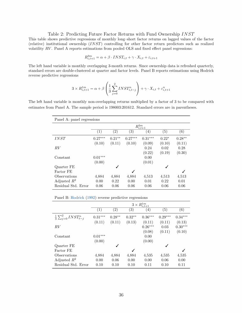
Table 2: Predicting Future Factor Returns with Fund Ownership INSTThis table shows predictive regressions of monthly long–short factor returns on lagged values of the factor(relative) institutional ownership (INST ) controlling for other factor return predictors such as realizedvolatility RV . Panel A reports estimations from pooled OLS and fixed effect panel regressions:

R3mi,t+1 = α+ β · INSTi,t + γ ·Xi,t + εi,t+1

The left hand variable is monthly overlapping 3-month returns. Since ownership data is refreshed quarterly,standard errors are double-clustered at quarter and factor levels. Panel B reports estimations using Hodrickreverse predictive regressions

3×R1mi,t+1 = α+ β

1

3

2∑j=0

INSTni,t−j

+ γ ·Xi,t + εni,t+1

The left hand variable is monthly non-overlapping returns multiplied by a factor of 3 to be compared with

estimates from Panel A. The sample period is 198003:201612. Standard errors are in parentheses.

Panel A: panel regressions

R3mi,t+1

(1) (2) (3) (4) (5) (6)

INST 0.27∗∗∗ 0.21∗∗ 0.27∗∗∗ 0.31∗∗∗ 0.22∗ 0.28∗∗

(0.10) (0.11) (0.10) (0.09) (0.10) (0.11)RV 0.24 0.02 0.28

(0.22) (0.19) (0.30)Constant 0.01∗∗∗ 0.00

(0.00) (0.01)Quarter FE 3 3Factor FE 3 3Observations 4,884 4,884 4,884 4,513 4,513 4,513Adjusted R2 0.00 0.22 0.00 0.01 0.22 0.01Residual Std. Error 0.06 0.06 0.06 0.06 0.06 0.06

Panel B: Hodrick (1992) reverse predictive regressions

3×R1mi,t+1

(1) (2) (3) (4) (5) (6)

13

∑2j=0 INST

nt−j 0.31∗∗∗ 0.28∗∗ 0.32∗∗ 0.36∗∗∗ 0.29∗∗∗ 0.34∗∗∗

(0.11) (0.11) (0.13) (0.11) (0.11) (0.13)RV 0.26∗∗∗ 0.03 0.30∗∗∗

(0.08) (0.11) (0.10)Constant 0.01∗∗∗ 0.00

(0.00) (0.00)Quarter FE 3 3Factor FE 3 3Observations 4,884 4,884 4,884 4,535 4,535 4,535Adjusted R2 0.00 0.06 0.00 0.00 0.06 0.00Residual Std. Error 0.10 0.10 0.10 0.11 0.10 0.11

36

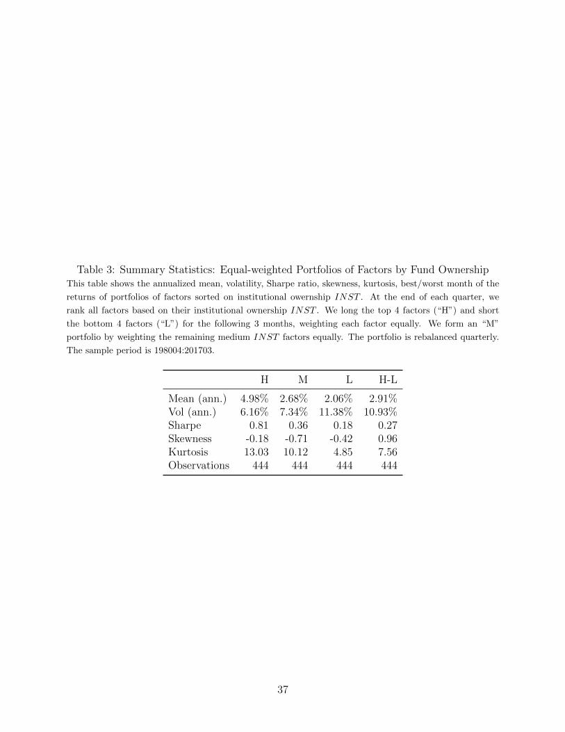
Table 3: Summary Statistics: Equal-weighted Portfolios of Factors by Fund OwnershipThis table shows the annualized mean, volatility, Sharpe ratio, skewness, kurtosis, best/worst month of the

returns of portfolios of factors sorted on institutional owernship INST . At the end of each quarter, we

rank all factors based on their institutional ownership INST . We long the top 4 factors (“H”) and short

the bottom 4 factors (“L”) for the following 3 months, weighting each factor equally. We form an “M”

portfolio by weighting the remaining medium INST factors equally. The portfolio is rebalanced quarterly.

The sample period is 198004:201703.

H M L H-L

Mean (ann.) 4.98% 2.68% 2.06% 2.91%Vol (ann.) 6.16% 7.34% 11.38% 10.93%Sharpe 0.81 0.36 0.18 0.27Skewness -0.18 -0.71 -0.42 0.96Kurtosis 13.03 10.12 4.85 7.56Observations 444 444 444 444

37

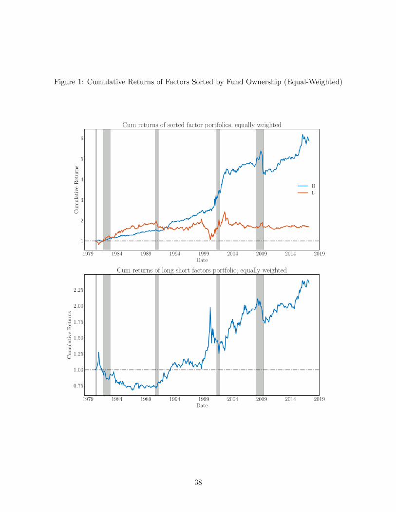
Figure 1: Cumulative Returns of Factors Sorted by Fund Ownership (Equal-Weighted)

1979 1984 1989 1994 1999 2004 2009 2014 2019Date

1

2

3

4

5

6

Cu

mu

lati

veR

etu

rns

Cum returns of sorted factor portfolios, equally weighted

H

L

1979 1984 1989 1994 1999 2004 2009 2014 2019Date

0.75

1.00

1.25

1.50

1.75

2.00

2.25

Cu

mu

lati

veR

etu

rns

Cum returns of long-short factors portfolio, equally weighted

38

Figure 2: 60-month Rolling Average of Factor Returns Sorted by Fund Ownership, (Equal-Weighted)

1984 1989 1994 1999 2004 2009 2014Date

−0.0075

−0.0050

−0.0025

0.0000

0.0025

0.0050

0.0075

0.0100

0.0125

Rol

lin

gR

etu

rns

60-month rolling returns of sorted factor portfolios, equally weighted

H

L

1984 1989 1994 1999 2004 2009 2014Date

−0.0075

−0.0050

−0.0025

0.0000

0.0025

0.0050

0.0075

0.0100

Rol

lin

gR

etu

rns

60-month rolling returns of long-short factors portfolio, equally weighted

39

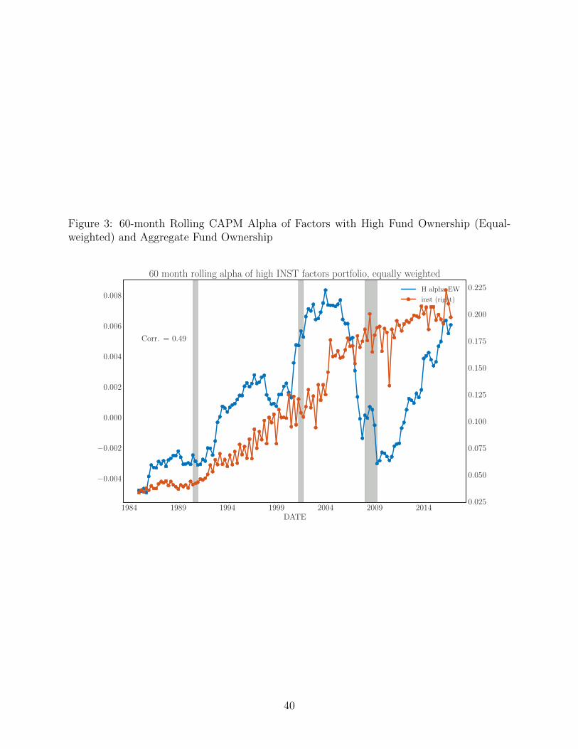
Figure 3: 60-month Rolling CAPM Alpha of Factors with High Fund Ownership (Equal-weighted) and Aggregate Fund Ownership

1984 1989 1994 1999 2004 2009 2014DATE

−0.004

−0.002

0.000

0.002

0.004

0.006

0.008

Corr. = 0.49

60 month rolling alpha of high INST factors portfolio, equally weighted

H alpha EW

inst (right)

0.025

0.050

0.075

0.100

0.125

0.150

0.175

0.200

0.225

40

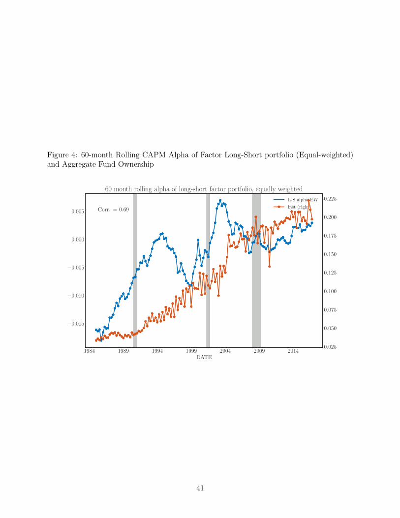
Figure 4: 60-month Rolling CAPM Alpha of Factor Long-Short portfolio (Equal-weighted)and Aggregate Fund Ownership

1984 1989 1994 1999 2004 2009 2014DATE

−0.015

−0.010

−0.005

0.000

0.005 Corr. = 0.69

60 month rolling alpha of long-short factor portfolio, equally weighted

L-S alpha EW

inst (right)

0.025

0.050

0.075

0.100

0.125

0.150

0.175

0.200

0.225

41

Figure 5: Model-implied and Detrended Empirical Fund Ownership δ

1982 1986 1990 1994 1998 2002 2006 2010 2014

−0.04

−0.02

0.00

0.02

0.04

Det

ren

ded

emp

iric

alδ

Corr. = 0.19

1982 1986 1990 1994 1998 2002 2006 2010 2014

−0.04

−0.02

0.00

0.02

HP

filt

ered

emp

iric

alδ

Corr. = 0.14

0.25

0.50

0.75

1.00

1.25

1.50

Bay

esia

nim

plied

δ

0.25

0.50

0.75

1.00

1.25

1.50

Bay

esia

nim

plied

δ

42

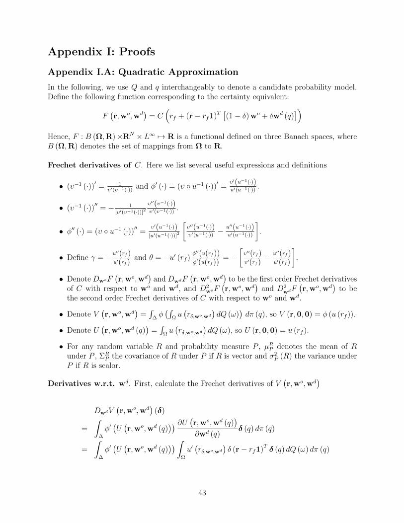
Appendix I: Proofs

Appendix I.A: Quadratic Approximation

In the following, we use Q and q interchangeably to denote a candidate probability model.Define the following function corresponding to the certainty equivalent:

F(r,wo,wd

)= C

(rf + (r− rf1)T

[(1− δ) wo + δwd (q)

])Hence, F : B (Ω,R)×RN ×L∞ 7→ R is a functional defined on three Banach spaces, whereB (Ω,R) denotes the set of mappings from Ω to R.

Frechet derivatives of C. Here we list several useful expressions and definitions

• (υ−1 (·))′ = 1υ′(υ−1(·)) and φ′ (·) = (υ u−1 (·))′ = υ′(u−1(·))

u′(u−1(·)) .

• (υ−1 (·))′′ = − 1[υ′(υ−1(·))]2

υ′′(υ−1(·))υ′(υ−1(·)) .

• φ′′ (·) = (υ u−1 (·))′′ = υ′(u−1(·))[u′(u−1(·))]2

[υ′′(u−1(·))υ′(u−1(·)) −

u′′(u−1(·))u′(u−1(·))

].

• Define γ = −u′′(rf)u′(rf)

and θ = −u′ (rf )φ′′(u(rf))φ′(u(rf))

= −[υ′′(rf)υ′(rf)

− u′′(rf)u′(rf)

].

• Denote DwoF(r,wo,wd

)and DwdF

(r,wo,wd

)to be the first order Frechet derivatives

of C with respect to wo and wd, and D2woF

(r,wo,wd

)and D2

wdF(r,wo,wd

)to be

the second order Frechet derivatives of C with respect to wo and wd.

• Denote V(r,wo,wd

)=∫

∆φ(∫

Ωu(rδ,wo,wd

)dQ (ω)

)dπ (q), so V (r,0,0) = φ (u (rf )).

• Denote U(r,wo,wd (q)

)=∫

Ωu(rδ,wo,wd

)dQ (ω), so U (r,0,0) = u (rf ).

• For any random variable R and probability measure P , µRP denotes the mean of Runder P , ΣR

P the covariance of R under P if R is vector and σ2P (R) the variance under

P if R is scalor.

Derivatives w.r.t. wd. First, calculate the Frechet derivatives of V(r,wo,wd

)DwdV

(r,wo,wd

)(δ)

=

∫∆

φ′(U(r,wo,wd (q)

)) ∂U (r,wo,wd (q))

∂wd (q)δ (q) dπ (q)

=

∫∆

φ′(U(r,wo,wd (q)

)) ∫Ω

u′(rδ,wo,wd

)δ (r− rf1)T δ (q) dQ (ω) dπ (q)

43

which is a row vector, and

D2wdV

(r,wo,wd

)(δ1, δ2)

=

∫∆

φ′′(U(r,wo,wd (q)

))(∫Ω

u′(rδ,wo,wd

)δ (r− rf1)T δ2 (q) dQ (ω)

)(∫

Ω

u′(rδ,wo,wd

)δ (r− rf1)T δ1 (q) dQ (ω)

)dπ (q) +

∫∆

φ′(U(r,wo,wd (q)

))∫

Ω

u′′(rδ,wo,wd

)δ2δ1 (q)T (r− rf1) (r− rf1)T δ2 (q) dQ (ω) dπ (q)

which is a N -by-N matrix. Evaluate at(wo,wd

)= 0 and δ = δ1 = δ1 = wd:

DwdV (r,0,0)(wd)

= υ′ (rf ) δEπ

(EQ

((r− rf1)T wd (q)

))D2

wdV (r,0,0) = φ′′ (u (rf )) [u′ (rf )]2δ2Eπ

([EQ

((r− rf1)T wd (q)

)]2)

+

φ′ (u (rf ))u′′ (rf )

(δ2)Eπ

(EQ

([(r− rf1)T wd (q)

]2))

By chain rule,

DwdF(r,wo,wd

)(δ) =

DwdV(r,wo,wd

)(δ)

υ′ (υ−1 (V (r,wo,wd)))

=

∫∆

φ′(U(r,wo,wd (q)

))υ′ (υ−1 (V (r,wo,wd)))

∫Ω

u′(rδ,wo,wd

)δ (r− rf1)T δ (q) dQ (ω) dπ (q)

D2wdF

(r,wo,wd

)(δ1, δ2) = − υ

′′ (υ−1(V(r,wo,wd

)))[υ′ (υ−1 (V (r,wo,wd)))]3

[DwdV

(r,wo,wd

)(δ1)

][DwdV

(r,wo,wd

)(δ2)

]+D2

wdV(r,wo,wd

)(δ1, δ2)

υ′ (υ−1 (V (r,wo,wd)))

Evaluate at(wo,wd

)= 0 and δ = δ1 = δ1 = wd:

DwdF (r,0,0)(wd)

= δEπ

(EQ

((r− rf1)T wd (q)

))D2

wdF (r,0,0)(wd,wd

)= −θδ2V arπ

(EQ

((r− rf1)T wd (q)

))−

γδ2Eπ

(σ2Q

((r− rf1)T wd (q)

))

44

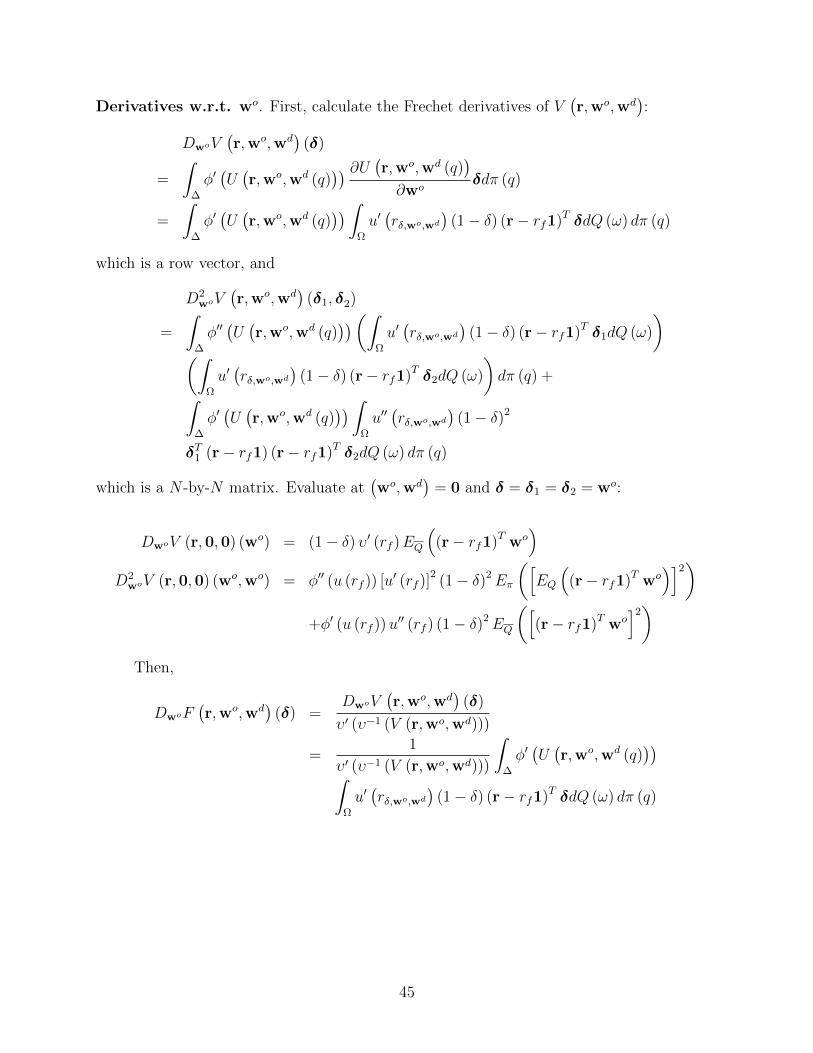
Derivatives w.r.t. wo. First, calculate the Frechet derivatives of V(r,wo,wd

):

DwoV(r,wo,wd

)(δ)

=

∫∆

φ′(U(r,wo,wd (q)

)) ∂U (r,wo,wd (q))

∂woδdπ (q)

=

∫∆

φ′(U(r,wo,wd (q)

)) ∫Ω

u′(rδ,wo,wd

)(1− δ) (r− rf1)T δdQ (ω) dπ (q)

which is a row vector, and

D2woV

(r,wo,wd

)(δ1, δ2)

=

∫∆

φ′′(U(r,wo,wd (q)

))(∫Ω

u′(rδ,wo,wd

)(1− δ) (r− rf1)T δ1dQ (ω)

)(∫

Ω

u′(rδ,wo,wd

)(1− δ) (r− rf1)T δ2dQ (ω)

)dπ (q) +∫

∆

φ′(U(r,wo,wd (q)

)) ∫Ω

u′′(rδ,wo,wd

)(1− δ)2

δT1 (r− rf1) (r− rf1)T δ2dQ (ω) dπ (q)

which is a N -by-N matrix. Evaluate at(wo,wd

)= 0 and δ = δ1 = δ2 = wo:

DwoV (r,0,0) (wo) = (1− δ) υ′ (rf )EQ(

(r− rf1)T wo)

D2woV (r,0,0) (wo,wo) = φ′′ (u (rf )) [u′ (rf )]

2(1− δ)2Eπ

([EQ

((r− rf1)T wo

)]2)

+φ′ (u (rf ))u′′ (rf ) (1− δ)2EQ

([(r− rf1)T wo

]2)

Then,

DwoF(r,wo,wd

)(δ) =

DwoV(r,wo,wd

)(δ)

υ′ (υ−1 (V (r,wo,wd)))

=1

υ′ (υ−1 (V (r,wo,wd)))

∫∆

φ′(U(r,wo,wd (q)

))∫

Ω

u′(rδ,wo,wd

)(1− δ) (r− rf1)T δdQ (ω) dπ (q)

45

and

D2woF

(r,wo,wd

)(δ1, δ2)

= − υ′′ (υ−1

(V(r,wo,wd

)))[υ′ (υ−1 (V (r,wo,wd)))]3

[DwoV

(r,wo,wd

)(δ1)

] [DwoV

(r,wo,wd

)(δ2)

]+D2

woV(r,wo,wd

)(wo,wo)

υ′ (υ−1 (V (r,wo,wd)))

Evaluate at(wo,wd

)= 0 and δ = δ1 = δ2 = wo:

DwoF (r,0,0) (wo) = (1− δ)(µrQ− rf1

)Two

D2woF (r,0,0) (wo,wo) = −θ (1− δ)2 V arπ

(EQ

((r− rf1)T wo

))−

γ (1− δ)2 V arQ

((r− rf1)T wo

)Second Derivatives w.r.t. wd and wo. Finally,

D2wowdF

(r,wo,wd

)(δ1, δ2)

=DwowdV

(r,wo,wd

)(δ1, δ2)

υ′ (υ−1 (V (r,wo,wd)))−[υ′′(υ−1

(V(r,wo,wd

)))/υ′(υ−1

(V(r,wo,wd

)))][υ′ (υ−1 (V (r,wo,wd)))]2[

DwoV(r,wo,wd

)(δ1)

] [DwdV

(r,wo,wd

)(δ2)

]Evaluate at

(wo,wd

)= 0 and δ1 = wo, δ2 = wd:

D2wowdF (r,0,0)

(wo,wd

)=

DwowdV (r,0,0)(wo,wd

)υ′ (rf )

− υ′′ (rf )

[υ′ (rf )]3 [DwoV (r,0,0) (wo)]

[DwdV (r,0,0)

(wd)]

where

DwowdV (r,0,0)(wo,wd

)= −υ′ (rf ) θ (1− δ) δ

∫∆

wd (q)T EQ (r− rf1)EQ

((r− rf1)T

)wodπ (q)

−υ′ (rf ) γ (1− δ) δ∫

∆

woTEQ

((r− rf1) (r− rf1)T

)wd (q) dπ (q)

46

Simplify the expression:

D2wowdF (r,0,0)

(wo,wd

)=

DwowdV (r,0,0)(wo,wd

)υ′ (rf )

− υ′′ (rf )

[υ′ (rf )]3 [DwoV (r,0,0) (wo)]

[DwdV (r,0,0)

(wd)]

= − (θ + γ) (1− δ) δcovπ(EQ

((r− rf1)T wo

), EQ

((r− rf1)T wd (q)

))−γ (1− δ) δEπ

(covQ

((r− rf1)T wo, (r− rf1)T wd (q)

))Taylor expansion of C. By Theorem 8.16 of Jost (2005),

C(rf + (r− rf1)T

[(1− δ) wo + δwd (q)

])= F

(r,wo,wd

)= rf +DwoF (r,0,0) (wo) +DwdF (r,0,0)

(wd)

+1

2D2

woF (r,0,0) (wo,wo) +1

2D2

wdF (r,0,0)(wd,wd

)+D2

wowdF (r,0,0)(wo,wd

)+R

(wo,wd

)where lim(wo,wd)→0

R(wo,wd)‖(wo,wd)‖2 = 0. We have calculatedDwdF (r,0,0), D2

wdF (r,0,0), DwoF (r,0,0),

D2woF (r,0,0), and D2

wowdF (r,0,0).To simplify the notations, let Rw denote the excess return generated by any portfolio w

and let RwP denotes the expected excess return of any portfolio w under probability measure

P . Also notice that wd (q) =(γΣr

Q

)−1 (µrQ − rf1

). We have:

Eπ

(covQ

(Rwo

, Rwd(q)))

= Eπ(woTΣr

Qwd (q))

=1

γ

(µrQ− rf1

)Two =

1

γRwo

Q

Taylor expansion can be simplified as

C(rf + (r− rf1)T

[(1− δ) wo + δwd (q)

])≈ rf + (1− δ)2Rwo

Q+ δEπ

(R

wd(q)Q

)− (θ + γ) (1− δ) δcovπ

(Rwo

Q , Rwd(q)Q

)−(1− δ)2

2

(γσ2

Q

(Rwo)

+ θσ2π

(Rwo

Q

))− δ2

2

(γEπ

(σ2Q

(Rwd(q)

))+ θσ2

π

(R

wd(q)Q

))Appendix I.B: Optimal Portfolio and Delegation

The investor’s problem ismaxwo,δ

C(rδ,wo,wd

)− δψ

given that

wd (q) =(γΣr

Q

)−1 (µrQ − rf1

)

47

Approximate C(rδ,wo,wd

):

C(rf + (r− rf1)T

[(1− δ) wo + δwd (q)

])≈ rf + (1− δ)2

(µrQ− rf1

)Two − (θ + γ) (1− δ) δcovπ

(µrQ − rf1, Rwd(q)

Q

)Two

−(1− δ)2

2

(γwoTΣr

Qwo + θwoTΣ

µrQπ wo

)+δEπ

(R

wd(q)Q

)− δ2

2

(γEπ

(σ2Q

(Rwd(q)

))+ θσ2

π

(R

wd(q)Q

))The first order condition of wo:

wo =(γΣr

Q+ θΣ

µrQπ

)−1[(µrQ− rf1

)− (θ + γ)

δ

1− δ covπ(µrQ, R

wd(q)Q

)]The first order condition of δ: δ equal to

γσ2Q

(Rwo)

+ θσ2π

(Rwo

Q

)+ Eπ

(R

wd(q)Q

)− 2Rwo

Q− (θ + γ) covπ

(Rwo

Q , Rwd(q)Q

)− ψ

γσ2Q

(Rwo) + θσ2π

(Rwo

Q

)+ Eπ

(R

wd(q)Q

)+ θσ2

π

(R

wd(q)Q

)− 2Rwo

Q− 2 (θ + γ) covπ

(Rwo

Q , Rwd(q)Q

)γσ2

Q

(Rwo)

+ θσ2π

(Rwo

Q

)can be simplified as

woT

[(µrQ− rf1

)− (θ + γ)

δ

1− δ covπ(µrQ, R

wd(q)Q

)]= Rwo

Q− (θ + γ)

δ

1− δ covπ(Rwo

Q , Rwd(q)Q

)So,

1− δ =θσ2

π

(R

wd(q)Q

)− (θ + γ) covπ

(Rwo

Q , Rwd(q)Q

)+ ψ

Eπ

(R

wd(q)Q

)+ θσ2

π

(R

wd(q)Q

)−Rwo

Q−(

2−δ1−δ

)(θ + γ) covπ

(Rwo

Q , Rwd(q)Q

)Divide both sides by 1− δ and rearrange: δ is equal to

Eπ

(R

wd(q)Q

)−Rwo

Q− (θ + γ) covπ

(Rwo

Q , Rwd(q)Q

)− ψ

Eπ

(R

wd(q)Q

)+ θσ2

π

(R

wd(q)Q

)−Rwo

Q− (θ + γ) covπ

(Rwo

Q , Rwd(q)Q

)

48

Appendix I.C: Analysis under the Simplified Ambiguity

Optimal delegation and portfolio. Under the assumption that π is Gaussian and ΣrP is

known, we have

covπ

(µrQ, R

wd(q)Q

)=

1

γcovπ

(µrQ − µr

Q,(µrQ − µr

Q

)T(Σr

P )−1(µrQ − µr

Q

))+

1

γcovπ

(µrQ − µr

Q,(µrQ − µr

Q

)T(Σr

P )−1(µrQ− rf1

))+

1

γcovπ

(µrQ − µr

Q,(µrQ− rf1

)T(Σr

P )−1 (µrQ − rf1

))Isserlis’ theorem implies

covπ

(µrkQ − µrk

Q,(µrQ − µr

Q

)T(Σr

P )−1(µrQ − µr

Q

))=∑i,j

(ΣrP )−1

(i,j)

(Eπ

[(µrkQ − µrk

Q

)(µriQ − µri

Q

)(µrjQ − µ

rj

Q

)]−Eπ

(µrkQ − µrk

Q

)E[(µriQ − µri

Q

)(µrjQ − µ

rj

Q

)])= 0

So,

covπ

(µrQ, R

wd(q)Q

)=

1

γcovπ

(µrQ − µr

Q,(µrQ − µr

Q

)T(Σr

P )−1(µrQ− rf1

))+

1

γcovπ

(µrQ − µr

Q,(µrQ − rf1

)T(Σr

P )−1(µrQ− rf1

))=

2

γ

(ΣµrQπ

)(Σr

P )−1(µrQ− rf1

)Under the assumption that Σ

µrQπ = υΣr

P , the investor’s portfolio is

wo

=(γΣr

Q+ θΣ

µrQπ

)−1[(µrQ− rf1

)− (θ + γ)

δ

1− δ covπ(µrQ, R

wd(q)Q

)]= (Σr

P )−1(µrQ− rf1

)[ 1

γ + υθ− υγ + υθ

γ + υθ

δ

1− δ2

γ

]with covπ

(µrQ, R

wd(q)Q

)= 2υ

γ

(µrQ− rf1

).

49

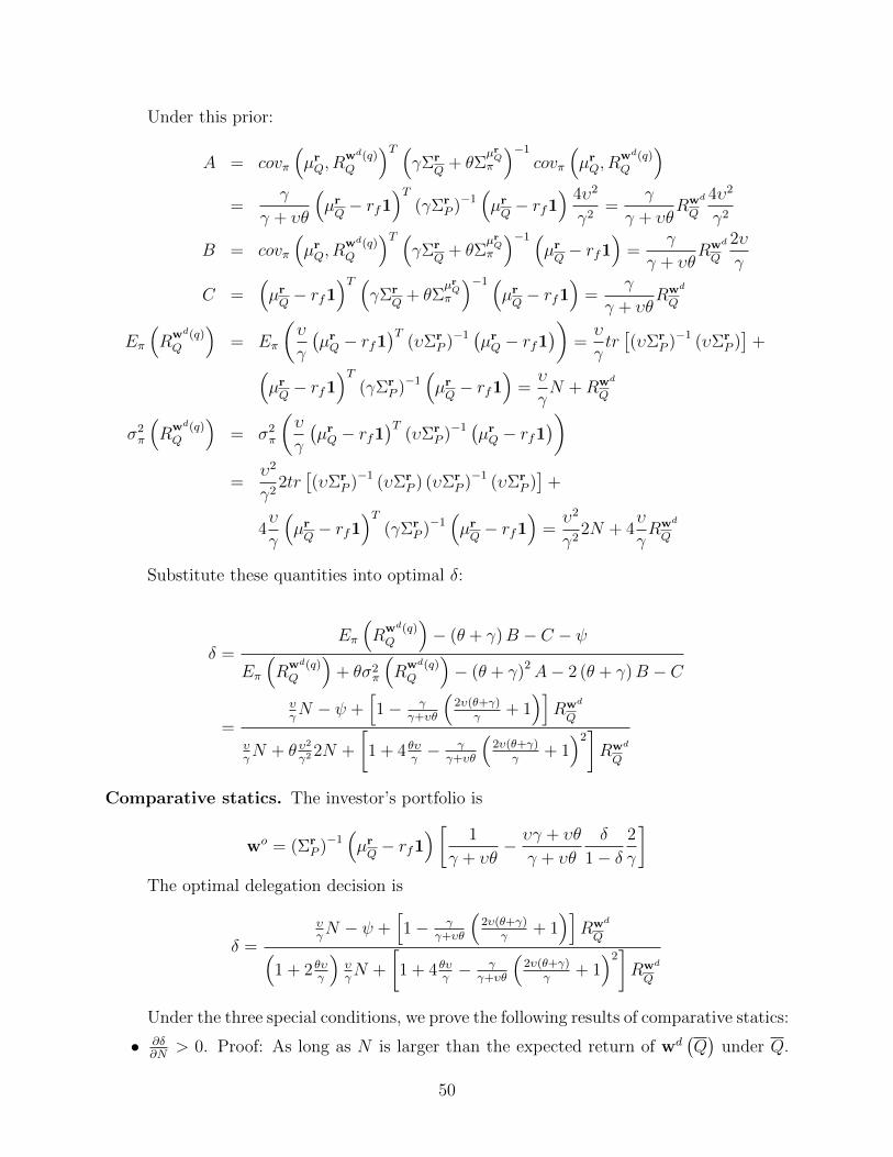
Under this prior:

A = covπ

(µrQ, R

wd(q)Q

)T (γΣr

Q+ θΣ

µrQπ

)−1

covπ

(µrQ, R

wd(q)Q

)=

γ

γ + υθ

(µrQ− rf1

)T(γΣr

P )−1(µrQ− rf1

) 4υ2

γ2=

γ

γ + υθRwd

Q

4υ2

γ2

B = covπ

(µrQ, R

wd(q)Q

)T (γΣr

Q+ θΣ

µrQπ

)−1 (µrQ− rf1

)=

γ

γ + υθRwd

Q

2υ

γ

C =(µrQ− rf1

)T (γΣr

Q+ θΣ

µrQπ

)−1 (µrQ− rf1

)=

γ

γ + υθRwd

Q

Eπ

(R

wd(q)Q

)= Eπ

(υ

γ

(µrQ − rf1

)T(υΣr

P )−1 (µrQ − rf1

))=υ

γtr[(υΣr

P )−1 (υΣrP )]

+(µrQ− rf1

)T(γΣr

P )−1(µrQ− rf1

)=υ

γN +Rwd

Q

σ2π

(R

wd(q)Q

)= σ2

π

(υ

γ

(µrQ − rf1

)T(υΣr

P )−1 (µrQ − rf1

))=

υ2

γ22tr[(υΣr

P )−1 (υΣrP ) (υΣr

P )−1 (υΣrP )]

+

4υ

γ

(µrQ− rf1

)T(γΣr

P )−1(µrQ− rf1

)=υ2

γ22N + 4

υ

γRwd

Q

Substitute these quantities into optimal δ:

δ =Eπ

(R

wd(q)Q

)− (θ + γ)B − C − ψ

Eπ

(R

wd(q)Q

)+ θσ2

π

(R

wd(q)Q

)− (θ + γ)2A− 2 (θ + γ)B − C

=

υγN − ψ +

[1− γ

γ+υθ

(2υ(θ+γ)

γ+ 1)]Rwd

Q

υγN + θ υ

2

γ22N +

[1 + 4 θυ

γ− γ

γ+υθ

(2υ(θ+γ)

γ+ 1)2]Rwd

Q

Comparative statics. The investor’s portfolio is

wo = (ΣrP )−1

(µrQ− rf1

)[ 1

γ + υθ− υγ + υθ

γ + υθ

δ

1− δ2

γ

]The optimal delegation decision is

δ =

υγN − ψ +

[1− γ

γ+υθ

(2υ(θ+γ)

γ+ 1)]Rwd

Q(1 + 2 θυ

γ

)υγN +

[1 + 4 θυ

γ− γ

γ+υθ

(2υ(θ+γ)

γ+ 1)2]Rwd

Q

Under the three special conditions, we prove the following results of comparative statics:

• ∂δ∂N

> 0. Proof: As long as N is larger than the expected return of wd(Q)

under Q.

50

Since δ ∈ (0, 1), δ increases in N :

2 θυγυγN + ψ +

[4 θυγ− 2υ(θ+γ)

γ+υθ

(2υ(θ+γ)

γ+ 1)]Rwd

Q(1 + 2 θυ

γ

)υγN +

[1 + 4 θυ

γ− γ

γ+υθ

(2υ(θ+γ)

γ+ 1)2]Rwd

Q

> 0

• ∂δ∂υ< 0, ∂δ

∂θ< 0 and ∂δ

∂γ> 0. As long as N is large enough, δ decreases in υ and θ, and

increases in γ:

δ =1 + γ

υN

(Rwd

Q− γ

γ+υθ

(2υ(θ+γ)

γ+ 1)Rwd

Q− ψ

)(

1 + 2 θυγ

)+

γRwd

Q

υN

(1 + 4 θυ

γ− γ

γ+υθ

(2υ(θ+γ)

γ+ 1)2)

• ∂wo

∂υ< 0, ∂wo

∂θ< 0 and ∂wo

∂γ< 0, conditional on δ. Proof: Note that υγ+υθ

γ+υθ= υγ+υθ

γ+υθ< 1

as long as υ < 1. Hence given δ, 1γ+υθ

− υγ+υθγ+υθ

δ1−δ

2γ

decreases in υ and θ.

∂ γ+θγ+υθ

1γ

∂γ=− (1− υ) θ

(γ + υθ)2

1

γ− 1

γ2

(γ + θ

γ + υθ

)< 0

as long as υ < 1.

• ∂wo

∂υ> 0, ∂wo

∂θ> 0, ∂wo

∂γ< 0 and

∂[ 1γ+υθ

−υγ+υθγ+υθ

δ1−δ

2γ ]γ

γ< 0. Proof: For large N ,

υθ+υγγ+υθ

(δ

1−δ

)≈ 1+γ/θ

1+υθ/γ12, so,

∂[

1γ+υθ

− υγ+υθγ+υθ

δ1−δ

2γ

]∂θ

≈2γ

2

θ2+ 22υγ

θ+ υ

(γ + υθ)2 > 0

∂[

1γ+υθ

− υγ+υθγ+υθ

δ1−δ

2γ

]∂υ

≈ θ + 2γ

(γ + υθ)2 > 0

∂[

1γ+υθ

− υγ+υθγ+υθ

δ1−δ

2γ

]∂γ

≈ −υ(γ + υθ)2 < 0

∂[

1γ+υθ

− υγ+υθγ+υθ

δ1−δ

2γ

]γ

∂γ≈ −

γ2

θ− 2γυ

(γ + υθ)2 < 0

51

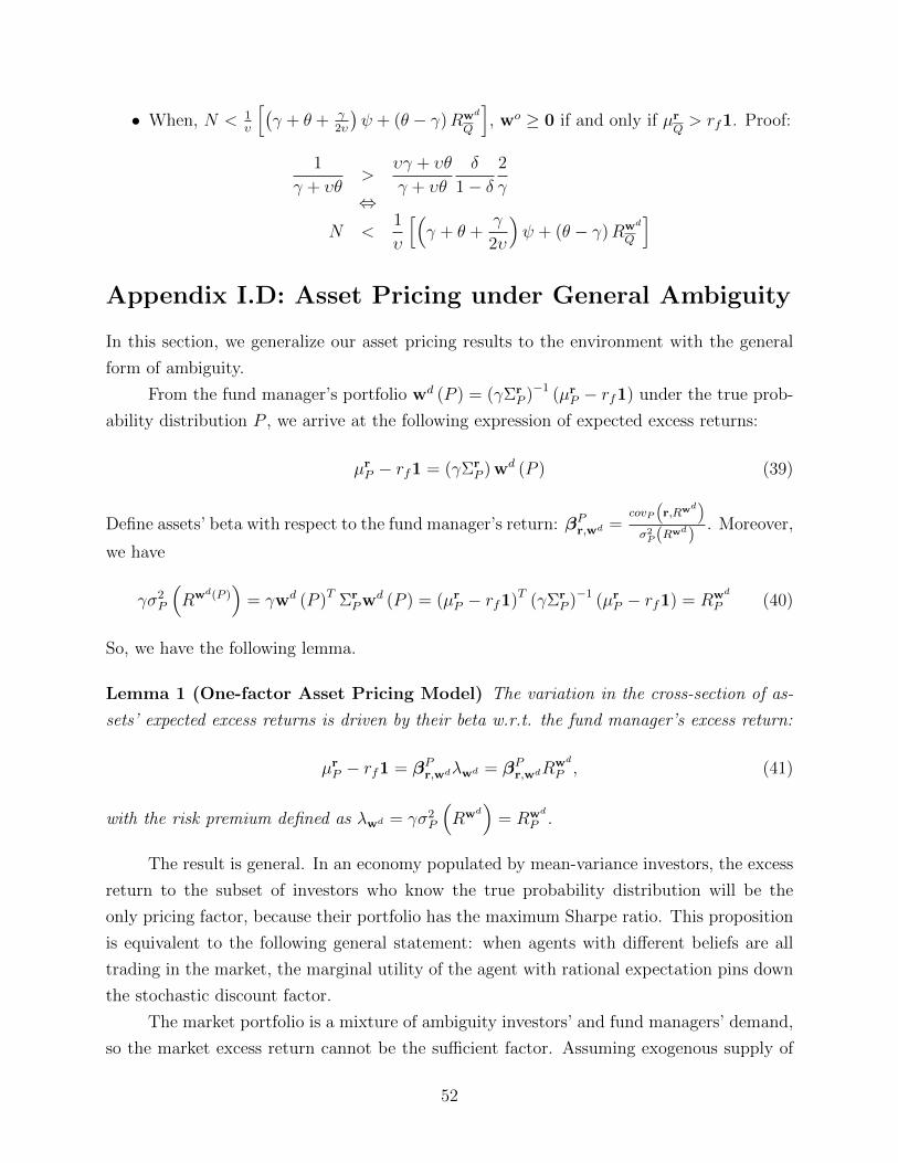
• When, N < 1υ

[(γ + θ + γ

2υ

)ψ + (θ − γ)Rwd

Q

], wo ≥ 0 if and only if µr

Q> rf1. Proof:

1

γ + υθ>

υγ + υθ

γ + υθ

δ

1− δ2

γ⇔

N <1

υ

[(γ + θ +

γ

2υ

)ψ + (θ − γ)Rwd

Q

]

Appendix I.D: Asset Pricing under General Ambiguity

In this section, we generalize our asset pricing results to the environment with the general

form of ambiguity.

From the fund manager’s portfolio wd (P ) = (γΣrP )−1 (µr

P − rf1) under the true prob-

ability distribution P , we arrive at the following expression of expected excess returns:

µrP − rf1 = (γΣr

P ) wd (P ) (39)

Define assets’ beta with respect to the fund manager’s return: βPr,wd =covP

(r,Rwd

)σ2P (Rwd)

. Moreover,

we have

γσ2P

(Rwd(P )

)= γwd (P )T Σr

Pwd (P ) = (µrP − rf1)T (γΣr

P )−1 (µrP − rf1) = Rwd

P (40)

So, we have the following lemma.

Lemma 1 (One-factor Asset Pricing Model) The variation in the cross-section of as-

sets’ expected excess returns is driven by their beta w.r.t. the fund manager’s excess return:

µrP − rf1 = βPr,wdλwd = βPr,wdRwd

P , (41)

with the risk premium defined as λwd = γσ2P

(Rwd

)= Rwd

P .

The result is general. In an economy populated by mean-variance investors, the excess

return to the subset of investors who know the true probability distribution will be the

only pricing factor, because their portfolio has the maximum Sharpe ratio. This proposition

is equivalent to the following general statement: when agents with different beliefs are all

trading in the market, the marginal utility of the agent with rational expectation pins down

the stochastic discount factor.

The market portfolio is a mixture of ambiguity investors’ and fund managers’ demand,

so the market excess return cannot be the sufficient factor. Assuming exogenous supply of

52

risky assets m (the market portfolio):

m = δwd (P ) + (1− δ) wo (42)

Substituting the market clearing condition into the equation of expected returns, we obtain:

µrP − rf1 = (γΣr

P )

[1

δm−

(1− δδ

)wo

]=(γδσ2P (Rm)

)βPr,m −

[(1− δ) γ

δσ2P

(Rwo)]

βPr,wo

where the market beta is βPr,m = covP (r, Rm) /σ2P (Rm), and the investor beta is βPr,wo =

covP(r, Rwo)

/σ2P

(Rwo)

. We have the following proposition.

Proposition 9 (CAPM Alpha with Delegation – General Ambiguity) Given the op-

timal delegation level δ, the equilibrium expected excess returns of risky assets are given by

µrP − rf1 = βPr,mλm + βPr,woλwo , (43)

where the premium on the market beta is λm = γδσ2P (Rm), and the premium on the investor

beta is λwo = −(

1−δδ

)γσ2

P

(Rwo)

.

The proposition links the CAPM alpha (α = βPr,woλwo) to the beta with respect to

the ambiguity investor’s portfolio return and the premium λwo . Since λwo < 0, an asset

whose return comoves with the return to the investor’s portfolio (βPr,wo > 0) lies below the

security market line, while an asset that moves against ambiguity investor’s portfolio delivers

positive alpha. This result looks a bit counter-intuitive. It seems that the ambiguity investors

should demand compensation for assets’ investor beta βPr,wo (i.e. λwo > 0) on top of the

standard market risk. However, the investors do not know the true probability distribution

P . Therefore, they cannot assess assets’ risk based on their betas.

The above analysis is general. It only requires a subset of market participants with

beliefs different from the true return distribution, who are the ambiguity investors in this

paper, and therefore, the analysis does not depend on the structure of investors’ ambiguity.

Next, we will relate the equilibrium asset returns to ambiguity more closely.

From Proposition 1 and market clearing condition m = δwd + (1− δ) wo, we have

µrP − rf1 = λmβ

Pr,m −

(1− δδ

)γΣr

Pwo (44)

where the market premium is defined in Proposition 9 λm = γδσ2P (Rm). We can link the

CAPM alpha −(

1−δδ

)γΣr

Pwo to ambiguity by substituting investors’ optimal portfolio choice

53

(Equation (??)) into the expected returns:

µrP − rf1 = λmβ

Pr,m +α (45)

where

α = ΣrP

(γΣr

Q+ θΣ

µrQπ

)−1

(θ + γ) γcovπ

(µrQ, R

wd(q)Q

)−

ΣrP

(γΣr

Q+ θΣ

µrQπ

)−1

γ(µrQ− rf1

)(1− δδ

)(46)

The next proposition decomposes the CAPM alpha into two components. More interest-

ingly, when the market is increasingly dominated by fund managers with the knowledge of

return distribution (rational expectation), the CAPM alpha does not disappear (even under

ambiguity neutrality θ = 1).

Proposition 10 (Alpha Decomposition – General Ambiguity) The CAPM alpha, α,

can be decomposed into the “ambiguity hedging” component

ΣrP

(γΣr

Q+ θΣ

µrQπ

)−1

(θ + γ) γcovπ

(µrQ, R

wd(q)Q

)(47)

and the “ambiguity participation” component,

− ΣrP

(γΣr

Q+ θΣ

µrQπ

)−1

γ(µrQ− rf1

)(1− δδ

)(48)

This proposition is the generalized version of Proposition 6. First, notice that under

ambiguity neutrality (θ = 0), the economy still deviates from CAPM (α 6= 0). This is be-

cause of the hedging demand induced by the cross-model covariation between the investment

opportunity set and the delegation return. Second, the ambiguity participation component

converges to zero, as the level of delegation δ approaches 1. Third, the ambiguity hedging

component is driven by investors’ hedge against the cross-model covariation between the

investment opportunity set (µrQ) and the delegation return (R

wd(q)Q ). This contrasts with the

CAPM alpha (λwo0βπµrQ,m) in Proposition 8. When delegation is unavailable, what matters

is the cross-model covariation between the investment opportunity set and investors’ own

portfolio return (which is also the market return). The following corollary is the generalized

version of Corollary 4.

Corollary 5 (Equilibrium Discontinuity with Delegation – General Ambiguity) As

δ approaches 100%, the equilibrium does not converge to the CAPM equilibrium, even under

54

ambiguity neutrality (θ = 0):

limδ→1

α = ΣrP

(γΣr

Q+ θΣ

µrQπ

)−1

(θ + γ) γcovπ

(µrQ, R

wd(q)Q

), (49)

and when θ = 0,

limδ→1

α = ΣrP

(ΣrQ

)−1

γcovπ

(µrQ, R

wd(q)Q

). (50)

55

References

Aguilar, Omar, and Mike West, 2000, Bayesian Dynamic Factor Models and Portfolio Allo-cation, Journal of Business and Economic Statistics 18, 338–357.

Andersen, Torben G., Tim Bollerslev, Peter F. Christoffersen, and Francis X. Diebold, 2006,Volatility and Correlation Forecasting , volume 1 of Handbook of Economic Forecasting ,chapter 15, 777–878.

Barras, Laurent, Olivier Scaillet, and Russ Wermers, 2010, False Discoveries in Mutual FundPerformance: Measuring Luck in Estimated Alphas, Journal of Finance 65, 179–216.

Bloom, Nicholas, 2009, The Impact of Uncertainty Shocks, Econometrica 77, 623–685.

Bossaerts, Peter, and Pierre Hillion, 1999, Implementing Statistical Criteria to Select ReturnForecasting Models: What Do We Learn? , Review of Financial Studies 12, 405–428.

Busse, Jeffrey A., 1999, Volatility Timing in Mutual Funds: Evidence from Daily Returns,Review of Financial Studies 12, 1009–1041.

Camerer, Colin, and Martin Weber, 1992, Recent Developments in Modeling Preferences:Uncertainty and Ambiguity, Journal of Risk & Uncertainty 5, 325–370.

Carhart, Mark M., 1997, On Persistence in Mutual Fund Performance, Journal of Finance52, 57–82.

Chen, Yong, and Bing Liang, 2007, Do Market Timing Hedge Funds Time the Market?,Journal of Financial and Quantitative Analysis 42, 827–856.

Del Guercio, Diane, and Jonathan Reuter, 2014, Mutual fund performance and the incentiveto generate alpha, Journal of Finance 69, 1673–1704.

Epstein, Larry G., 2010, Three Paradoxes for the “Smooth Ambiguity” Model of Preference,Econometrica 78, 20852099.

Epstein, Larry G., and Stanley E. Zin, 1989, Substitution, Risk Aversion, and the TemporalBehavior of Consumption and Asset Returns: A Theoretical Framework, Econometrica57, 937–969.

Fama, Eugene F., and Kenneth R. French, 1993, Common risk factors in the returns onstocks and bonds, Journal of Financial Economics 33, 3–56.

Fama, Eugene F., and Kenneth R. French, 2010, Luck Versus Skill in the Cross-Section ofMutual Fund Alpha Estimates, Journal of Finance 65, 1915–1947.

Ferson, Wayne, and Haitao Mo, 2016, Performance measurement with selectivity, marketand volatility timing, Journal of Financial Economics 121, 93 – 110.

Ferson, Wayne E., and Rudi W. Schadt, 1996, Measuring Fund Strategy and Performancein Changing Economic Conditions, Journal of Finance 51, 425–462.

56

French, Kenneth R., 2008, Presidential Address: The Cost of Active Investing, Journal ofFinance LXIII.

Garlappi, Lorenzo, Raman Uppal, and Tan Wang, 2007, Portfolio Selection with Parameterand Model Uncertainty: A Multi-Prior Approach, Review of Financial Studies 20, 41–81.

Gruber, Martin J., 1996, Another Puzzle: The Growth in Actively Managed Mutual Funds,Journal of Finance 51, 783–810.

Guidolin, Massimo, and Francesca Rinaldi, 2010, Ambiguity in Asset Pricing and PortfolioChoice: A Review of the Literature, Working paper, Federal Reserve Bank of St. Louis.

Hansen, Lars Peter, and Thomas J. Sargent, 2012, Three types of ambiguity, Journal ofMonetary Economics 59, 422 – 445, Carnegie-NYU-Rochester Conference Series on PublicPolicy - Robust Macroeconomic Policy at Carnegie Mellon University on November 11-12,2011.

Hansen, Lars Peter, and Thomas J. Sargent, 2016, Robustness , reprint edition (PrincetonUniversity Press, Princeton, N.J.).

Henriksson, Roy D., 1984, Market Timing and Mutual Fund Performance: An EmpiricalInvestigation, Journal of Business 57, 73–96.

Hodrick, Robert J., 1992, Dividend Yields and Expected Stock Returns: Alternative Proce-dures for Inference and Measurement, Review of Economic Dynamics 5, 357–386.

Jacquier, Eric, Nicholas G. Polson, and Peter Rossi, 1999, Stochastic Volatility: Univariateand Multivariate Extensions, in Christopher F. Baum, ed., Computing in Economics andFinance, volume 112.

Jagannathan, Ravi, Ellen R. McGrattan, and Anna Scherbina, 2001, The declining u.s.equity premium, Working Paper 8172, National Bureau of Economic Research.

Jensen, Michael C., 1968, The Performance of Mutual Funds in the Period 1945-1964, Journalof Finance 23, 389–416.

Johannes, Michael, Arthur Korteweg, and Nicholas Polson, 2014, Sequential learning, pre-dictability, and optimal portfolio returns, Journal of Finance 69, 611–644.

Jondeau, Eric, and Michael Rockinger, 2012, On the Importance of Time-Variability inHigher Moments for Asset Allocation, Journal of Financial Econometrics 10, 84–123.

Jost, Jurgen, 2005, Postmodern Analysis (Springer, Germany).

Ju, Nengjiu, and Jianjun Miao, 2012, Ambiguity, Learning, and Asset Returns, Econometrica80, 559–591.

Klibanoff, Peter, Massimo Marinacci, and Sujoy Mukerji, 2005, A smooth model of decisionmaking under ambiguity, Econometrica 73, 1849–1892.

57

Klibanoff, Peter, Massimo Marinacci, and Sujoy Mukerji, 2012, On the Smooth AmbiguityModel: A Reply, Econometrica 80, 1303–1321.

Knight, Frank H., 1921, Risk, Uncertainty, and Profit (Houghton Mifflin Co., Boston, MA).

Kogan, Leonid, and Tan Wang, 2003, Simple Theory of Asset Pricing under Model Uncer-tainty, Working paper, MIT.

Lettau, Martin, Sydney C. Ludvigson, and Jessica A. Wachter, 2008, The declining equitypremium: What role does macroeconomic risk play?, The Review of Financial Studies 21,1653–1687.

Lewellen, Jonathan, 2010, Institutional Investors and the Limits of Arbitrage, Journal ofFinancial Economics 102, 62–80.

Maccheroni, Fabio, Massimo Marinacci, and Doriana Ruffino, 2013, Alpha as Ambiguity:Robust Mean-Variance Portfolio Analysis, Econometrica 81, 1075–1113.

Maenhout, Pascal J., 2004, Robust Portfolio Rules and Asset Pricing, Review of FinancialStudies 17, 951–983.

Malkiel, Burton, 1995, Returns from Investing in Equity Mutual Funds 1971 to 1991, Journalof Finance 50, 549–572.

Markowitz, Harry M., 1959, Portfolio Selection: Efficient Diversification of Investments(Wiley, New York, NY).

Marquering, Wessel, and Marno Verbeek, 2004, The Economic Value of Predicting StockIndex Returns and Volatility, Journal of Financial and Quantitative Analysis 39, 407–429.

Merton, Robert C., 1980, On Estimating the Expected Return on the Market: An Explana-tory Investigation, Journal of Financial Economics 8, 323–361.

Moreira, Alan, and Tyler Muir, 2017, Volatility-managed portfolios, The Journal of Finance72, 1611–1644.

Nagel, Stefan, 2005, Short sales, institutional investors and the cross-section of stock returns,Journal of Financial Economics 78, 277 – 309.

Pesaran, M. Hashem, and Allan Timmermann, 1995, Predictability of Stock Returns: Ro-bustness and Economic Significance, Journal of Finance 50, 1201–1228.

Segal, Uzi, 1990, Two-Stage Lotteries without the Reduction Axiom, Econometrica 58, 349–377.

Strzalecki, Tomasz, 2013, Temporal resolution of uncertainty and recursive models of ambi-guity aversion, Econometrica 81, 1039–1074.

58

Wakker, Peter P., 2008, Uncertainty, in Steven N. Durlauf, and Lawrence E. Blume, eds.,The New Palgrave Dictionary of Economics (Palgrave Macmillan).

Wermers, Russ, 2000, Mutual Fund Performance: An Empirical Decomposition into Stock-Picking Talent, Style, Transactions Costs, and Expenses, Journal of Finance 55, 1655–1703.

59