Delay in Strategic Information Aggregation

Ettore Damiano

University of Toronto

Li, Hao

University of Toronto

Wing Suen

The University of Hong Kong

October 24, 2007

Abstract. We study a model of collective decision making in which divergent preferences

of the agents make information aggregation impossible in a single round of voting. With

costly delay, we show that repeated voting can help the agents reach a mutually preferred

decision, even though there is no new direct information about the decision between two

rounds of voting. An increase in the cost of delay can improve the efficiency of information

aggregation, and hence the ex ante welfare of the agents involved, by encouraging the

agents to be more forthcoming with their private information in the initial rounds of

voting. Allowing an additional round of voting in case of disagreements can similarly

improve the ex ante welfare when there is an intermediate degree of conflict, but reduces

the welfare otherwise. With sufficiently many rounds of voting allowed, the equilibrium

play of the repeated voting game involves gradually increasing concessions.

Notes. This is a preliminary draft. Please do not circulate without permission. Suen

and Li thank Guanghua School of Management of Beijing University, and especially the

Department of Applied Economics and its chair Hongbin Cai, for their hospitality and

research support during their visit. Li wishes to thank the Marshall School of Business of

the University of Southern California for hosting his sabbatical when part of the research

for this paper is done.

– i –

presented by Li, HaoFRIDAY, Oct. 26, 20071:30 pm – 3:00 pm, Room: HOH-706

USC FBE APPLIED ECONOMICS WORKSHOP

1. Introduction

Individuals may disagree with one another when they have different preferences or when

they have different private information. Often, it is difficult to distinguish between these

two types of disagreement because divergent preferences provide incentives for individuals

to distort their information. Even though they may share a common interest in some

states had the individuals known each other’s private information, the strategic distortion

of information can still cause disagreement in these states. If disagreements lead to delay

in making decisions, then it often seems that any decision is better than no decision and

costly delay. For example, people complain about legislative deadlock and the delay costs

it entails. We argue in this paper, however, that institutionalized delay in the decision

making process can serve a useful purpose. In the context of a stylized model of repeated

voting, the prospect of costly delay induces the parties to be more accommodating in the

initial rounds of voting and enhances information aggregation. As a result, a greater delay

cost between two rounds of voting can lead to an improvement in the ex ante welfare of

the decision makers.

The problem of disagreement that we study resembles but is not identical to a pure

bargaining problem. The two decision makers in our model have private information about

which is the appropriate alternative to adopt. If they could perfectly aggregate their

private information, there are some states of the world in which they still would disagree

because of divergent preferences but there are also some states of the world in which they

would agree. Therefore the role of delay described in this paper is different from that in a

pure bargaining model (Stahl 1972; Rubinstein 1982). In the Stahl-Rubinstein bargaining

model, the trade off between getting a bigger share of the pie but at a later date helps pin

down a unique solution to the bargaining problem which is plagued by multiple equilibria

in a one-shot model. One feature of the Stahl-Rubinstein model is that delay does not

occur in equilibrium: the mere possibility of incurring delay cost helps prompt the two

bargaining parties to reach an agreement in the first round. In our setting, the one-round

voting game has a generically unique equilibrium, and the repeated voting game entails a

different outcome with delay occurring in equilibrium.

– 1 –

There are numerous extensions to the Stahl-Rubinstein model that can generate delay

as part of the equilibrium outcome. One strand of this literature relies on asymmetric

information about the size of the pie that is being divided.1 In a model of strikes, for

example, a firm knows its own profitability but the firm’s unionized workforce does not.

Strike or delay is a signaling device in the sense that the willingness to endure a longer

work stoppage can credibly signal the firm’s low profitability and help it to arrive at a more

favorable wage bargain. In this type of signaling models, each agent’s gains from trade at a

given price depend only on his own private information. In our model, disagreement over

the alternatives is not a pure bargaining issue, because individuals in our model would

sometimes agree on which is the best alternative had they known the true state. Put

differently, voting outcomes in our setup determine the size as well as the division of the

pie. We show that delay can play a constructive role in overcoming disagreement improving

the ex ante welfare of all individuals.

Our paper is also related to the literature on debates (Austen-Smith 1990; Austen-

Smith and Feddersen 2006; Ottaviani and Sorensen 2001) and voting (Li, Rosen and Suen

2001) in committees.2 Models of debate typically analyze repeated information transmis-

sion as cheap talk, while we emphasize the role of delay cost in multiple rounds of voting.

Our setup is the closest to the Li, Rosen and Suen paper. The focus there is on the im-

possibility of efficient information aggregation. Here, we have intentionally skirted issues

such as quality of private signals and the trade-off between making the two different types

of errors. We focus instead on how delay and multiple voting rounds can help improve

information aggregation in a simple environment.

Section 2 introduces the information structure and the preferences of two individuals in

a symmetric strategic information aggregation problem with two alternatives. There is one

disagreement state in which each of the two individuals prefers his own favorite alternative

1 See, for example, Chatterjee and Samuelson (1987), Cho (1990), Cramton (1992), and Kennan andWilson (1993). There are also bargaining models that generate equilibrium delay under complete informa-tion, through commitment to not accepting offers poorer than past rejected ones (Freshtman and Seidmann1993), simultaneous offers (Sakovic 1993), and multi-lateral negotiations (Cai 2000).

2 Coughlan (2000) investigates conditions under which jurors vote their signals and their informationis efficiently aggregated in a model where a mistrial leads to a retrial by a new independent jury. He doesnot consider the issues of delay that are the focus of the present paper.

– 2 –

if they knew this was the true state, and one agreement state for each alternative, with

the degree of conflict between the two individuals captured by the prior probability of

disagreement state. Each individual is either a “extremist,” whose private signal is that

the state is the agreement state corresponding to his favorite alternative, or a “moderate,”

who knows only that the the state is either the other agreement state or the disagreement

state. As a benchmark for models with delay, we first consider a game with a single

round of voting between the two alternatives, in which two agreeing votes lead to the

agreed alternative being chosen and disagreeing votes result in a coin flip between the

two alternatives. The equilibrium outcome is generically either an efficient aggregation of

the private information through informative voting when the degree of conflict is low, or

otherwise a coin flip due to uninformative voting. In the latter case, we show that without

the possibility of delay, there is no incentive compatible outcome that Pareto dominates

the coin flip.

Section 3 allows the two individuals to vote for a second time after paying a delay

cost, if they disagree in the first round of voting. There is a unique equilibrium outcome, in

which the option of voting again in case of disagreement makes the voting by the moderate

types less informative in the first round when the degree of conflict is low, but has the

opposite effect when the degree of conflict is high. In the latter case, the softening of the

positions taken by the moderate types improves information aggregation in the first round

voting. It turns out that the effect of delay cost on the ex ante welfare of the decision

makers is non-monotone. Small delay cost does not help resolve disagreement while large

delay cost facilitates good decisions at too high a price. There is an intermediate range

of delay cost that improves the ex ante welfare of decision makers over a single round of

voting.

In section 4 we extend the analysis to games with a finite deadline that may involve

more than two rounds of voting, and a game without a deadline so that a disagreement

always leads to another round of voting. We show that a longer deadline can increase the

ex ante welfare when the degree of conflict is at intermediate levels but otherwise decreases

the welfare. An implication is that the “optimal deadline” from the ex ante point of view

is positive for intermediate degrees of conflict but zero when the degree of conflict is either

– 3 –

too low or too high. In the game without a deadline, as in the game with possibly two

rounds of voting, an increase in the delay cost leads to a softening of the positions taken

by the moderate types for all levels of conflict. However, unlike the game with possibly

two rounds of voting, when the deadline is sufficiently long, his willingness to compromise

depends negatively on the degree of conflict. As a result, the equilibrium play has the

intuitive feature of gradually increasing concessions: the moderate types start out with

a tough position, and each disagreement resulting from both individuals voting for their

favorite alternatives leads to a less pessimistic belief that the state is the disagreement

state, and hence to a softening of his position. Section 5 concludes the paper with some

discussion of interesting issues that remain to be investigated.

2. The Model

2.1. Information and preferences

Two players have to make a public choice between two alternatives, c and p. For conve-

nience, we call one player a conservative (player C) and the other a progressive (player

P ). There are three possible states of the world: R, M , and L. The corresponding prior

probabilities are denoted πR, πM , and πL. Our mode is intentionally symmetric; we there-

fore assume that πR = πL = π and πM = 1− 2π. The information structure is as follows:

the conservative is able to distinguish whether the state is R or not, while the progres-

sive is able to distinguish whether the state is L or not. Such information is private and

unverifiable.

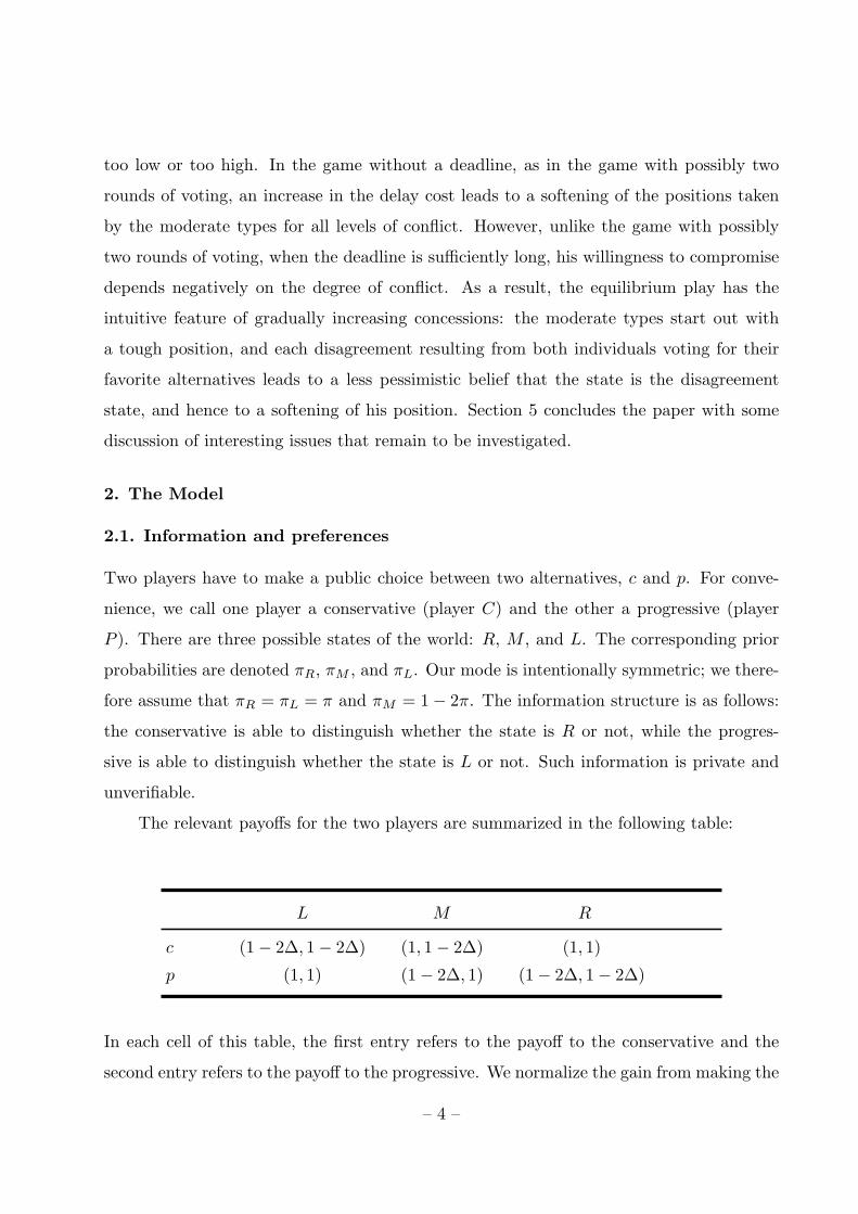
The relevant payoffs for the two players are summarized in the following table:

L M R

c (1− 2∆, 1− 2∆) (1, 1− 2∆) (1, 1)

p (1, 1) (1− 2∆, 1) (1− 2∆, 1− 2∆)

In each cell of this table, the first entry refers to the payoff to the conservative and the

second entry refers to the payoff to the progressive. We normalize the gain from making the

– 4 –

preferred decision to 1 and let the payoff from making the less preferred decision be 1−2∆.

The parameter ∆ > 0 is the error cost, or the cost of making the wrong decision. In state

R both players prefer c to p, and in state L both prefer p to c. The two players’ preferences

are different when the state is M : the conservative prefers c while the progressive prefers

p. Thus in our model there are elements of both common interest and conflict between

these two players.

A conservative who knows that the state is R prefers c to p, and is referred to as an

“extreme conservative.” A progressive who knows that the state is L prefers p to c, and is

called an “extreme progressive.”3 The preference between c and p of a conservative who

knows that the state is either L or M depends on the relative likelihood of these states.

Let γ denote his belief that the state is M . We have

γ =πM

πL + πM=

1− 2π

2π.

If the conservative could dictate the outcome, he strictly prefers c to p if and only if

γ + (1− γ)(1− 2∆) > γ(1− 2∆) + (1− γ),

which is equivalent to γ > 12 . We designate him as a “moderate conservative.” Similarly,

because of the assumption that πR = πL, a progressive with the signal that the state is not

L also has belief γ that the state is M . He strictly prefers p to c if and only if γ > 12 . We

designate him as a “moderate progressive.” In our later analysis of games with repeated

voting, given that there is no exogenous new information, the designations of extremists

and moderates do not change.

We note that γ can be interpreted as the ex ante degree of conflict. When γ is high, a

moderate player perceives that his opponent is likely to have different preferences regarding

the correct decision to be chosen. In the following analysis of games with repeated voting,

the belief of the moderate types, and hence the degree of conflict, changes endogenously

as voting progresses.

3 In our model an extremist is informed of the Pareto optimal decision, rather than someone with alarge bias for his favorite choice that may not be overcome with contrary evidence as in many models ofstrategic communication or voting.

– 5 –

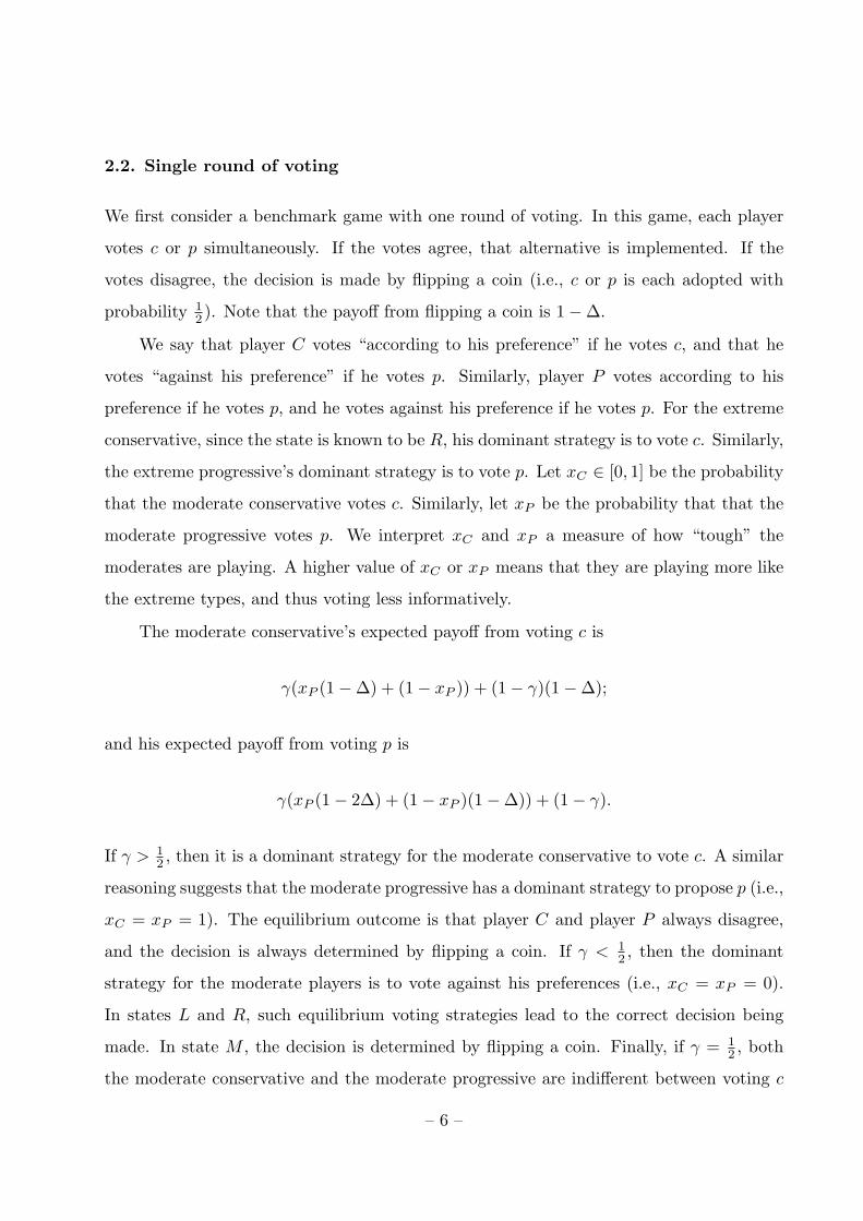
2.2. Single round of voting

We first consider a benchmark game with one round of voting. In this game, each player

votes c or p simultaneously. If the votes agree, that alternative is implemented. If the

votes disagree, the decision is made by flipping a coin (i.e., c or p is each adopted with

probability 12 ). Note that the payoff from flipping a coin is 1−∆.

We say that player C votes “according to his preference” if he votes c, and that he

votes “against his preference” if he votes p. Similarly, player P votes according to his

preference if he votes p, and he votes against his preference if he votes p. For the extreme

conservative, since the state is known to be R, his dominant strategy is to vote c. Similarly,

the extreme progressive’s dominant strategy is to vote p. Let xC ∈ [0, 1] be the probability

that the moderate conservative votes c. Similarly, let xP be the probability that that the

moderate progressive votes p. We interpret xC and xP a measure of how “tough” the

moderates are playing. A higher value of xC or xP means that they are playing more like

the extreme types, and thus voting less informatively.

The moderate conservative’s expected payoff from voting c is

γ(xP (1−∆) + (1− xP )) + (1− γ)(1−∆);

and his expected payoff from voting p is

γ(xP (1− 2∆) + (1− xP )(1−∆)) + (1− γ).

If γ > 12 , then it is a dominant strategy for the moderate conservative to vote c. A similar

reasoning suggests that the moderate progressive has a dominant strategy to propose p (i.e.,

xC = xP = 1). The equilibrium outcome is that player C and player P always disagree,

and the decision is always determined by flipping a coin. If γ < 12 , then the dominant

strategy for the moderate players is to vote against his preferences (i.e., xC = xP = 0).

In states L and R, such equilibrium voting strategies lead to the correct decision being

made. In state M , the decision is determined by flipping a coin. Finally, if γ = 12 , both

the moderate conservative and the moderate progressive are indifferent between voting c

– 6 –

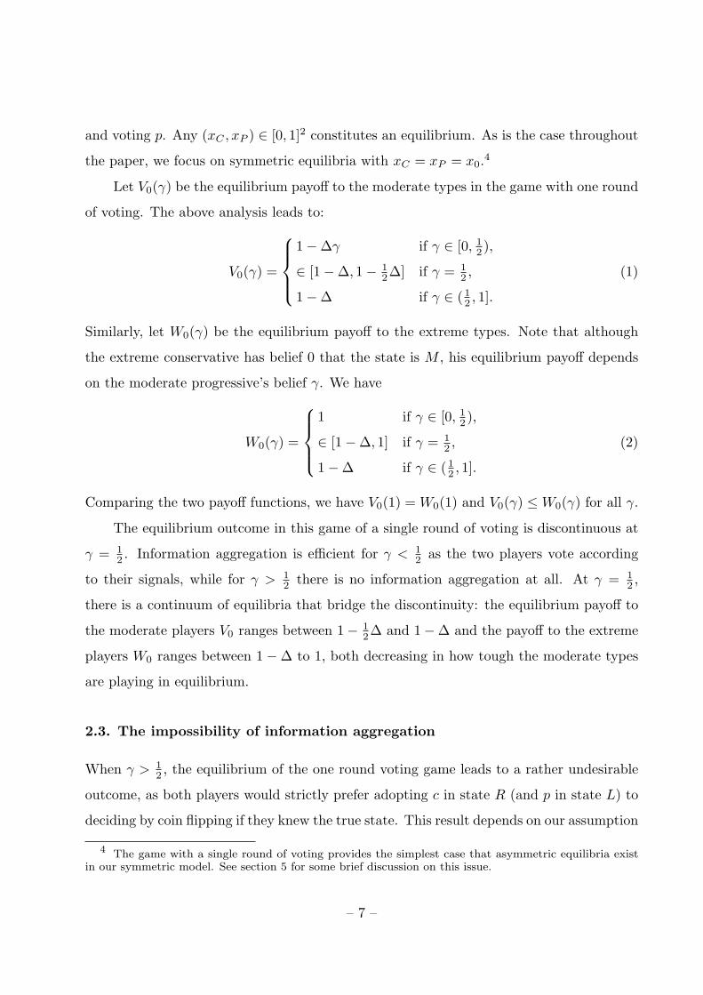
and voting p. Any (xC , xP ) ∈ [0, 1]2 constitutes an equilibrium. As is the case throughout

the paper, we focus on symmetric equilibria with xC = xP = x0.4

Let V0(γ) be the equilibrium payoff to the moderate types in the game with one round

of voting. The above analysis leads to:

V0(γ) =

1−∆γ if γ ∈ [0, 12 ),

∈ [1−∆, 1− 12∆] if γ = 1

2 ,

1−∆ if γ ∈ ( 12 , 1].

(1)

Similarly, let W0(γ) be the equilibrium payoff to the extreme types. Note that although

the extreme conservative has belief 0 that the state is M , his equilibrium payoff depends

on the moderate progressive’s belief γ. We have

W0(γ) =

1 if γ ∈ [0, 12 ),

∈ [1−∆, 1] if γ = 12 ,

1−∆ if γ ∈ ( 12 , 1].

(2)

Comparing the two payoff functions, we have V0(1) = W0(1) and V0(γ) ≤ W0(γ) for all γ.

The equilibrium outcome in this game of a single round of voting is discontinuous at

γ = 12 . Information aggregation is efficient for γ < 1

2 as the two players vote according

to their signals, while for γ > 12 there is no information aggregation at all. At γ = 1

2 ,

there is a continuum of equilibria that bridge the discontinuity: the equilibrium payoff to

the moderate players V0 ranges between 1− 12∆ and 1−∆ and the payoff to the extreme

players W0 ranges between 1−∆ to 1, both decreasing in how tough the moderate types

are playing in equilibrium.

2.3. The impossibility of information aggregation

When γ > 12 , the equilibrium of the one round voting game leads to a rather undesirable

outcome, as both players would strictly prefer adopting c in state R (and p in state L) to

deciding by coin flipping if they knew the true state. This result depends on our assumption

4 The game with a single round of voting provides the simplest case that asymmetric equilibria existin our symmetric model. See section 5 for some brief discussion on this issue.

– 7 –

about the structure of the voting game. We can obtain different outcomes by changing the

rules of the voting game. For example, suppose the rule is that player C is the decisive

voter. Then it is still a Nash equilibrium for player C to vote c and for player P to vote p

regardless of their private information. The ex ante equilibrium payoff of the conservative

(before observing his private information) is 1 − 2πL∆ while the ex ante payoff of the

progressive is 1−2(πR +πM )∆. In this case, changing the rule of the voting game benefits

the conservative player but hurts the progressive player compared to our benchmark game

in the previous subsection. However the unweighted sum of equilibrium payoffs for these

two players remains the same as in the benchmark case.

More generally, we can ask if it is possible to improve on the benchmark outcome

using some other mechanism without side transfers. By the revelation principle, it suffices

to consider any direct mechanism which satisfies the incentive compatibility constraints

for truthful reporting of private signals. In a truth-telling equilibrium, the true state can

be recovered from the reports submitted by the conservative and progressive players. For

example, if both player C and player P report that they are moderate types, then the true

state must be M . Let qR, qM , and qL be the probabilities of implementing alternative c

when the true state is R, M , and L, respectively. Let q be the probability of implementing

c when the reports are inconsistent, that is, when both C and P report that they are

extreme types. The incentive constraints can be written as:

qR + (1− qR)(1− 2∆) ≥ qM + (1− qM )(1− 2∆),

qL(1− 2∆) + (1− qL) ≥ qM (1− 2∆) + (1− qM ),

γ(qM + (1− qM )(1− 2∆)) + (1− γ)(qL(1− 2∆) + (1− qL))

≥ γ(qR + (1− qR)(1− 2∆)) + (1− γ)(q(1− 2∆) + (1− q)),

γ(qM (1− 2∆) + (1− qM )) + (1− γ)(qR + (1− qR)(1− 2∆))

≥ γ(qL(1− 2∆) + (1− qL)) + (1− γ)(q + (1− q)(1− 2∆)).

(3)

The first inequality is the incentive constraint for the extreme conservative. The left

side of this inequality is his expected payoff if he reports the truth. If he lies and reports

that he is a moderate instead, since the moderate progressive truthfully reports his type,

the state is taken to be M and the extreme conservative’s payoff is given by the right

– 8 –

side of the inequality. The other three inequalities are the truth-telling conditions for the

extreme progressive, the moderate conservative and the moderate progressive respectively,

and can be understood in an similar manner.

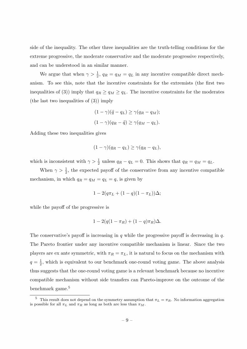
We argue that when γ > 12 , qR = qM = qL in any incentive compatible direct mech-

anism. To see this, note that the incentive constraints for the extremists (the first two

inequalities of (3)) imply that qR ≥ qM ≥ qL. The incentive constraints for the moderates

(the last two inequalities of (3)) imply

(1− γ)(q − qL) ≥ γ(qR − qM );

(1− γ)(qR − q) ≥ γ(qM − qL).

Adding these two inequalities gives

(1− γ)(qR − qL) ≥ γ(qR − qL),

which is inconsistent with γ > 12 unless qR − qL = 0. This shows that qR = qM = qL.

When γ > 12 , the expected payoff of the conservative from any incentive compatible

mechanism, in which qR = qM = qL = q, is given by

1− 2(qπL + (1− q)(1− πL))∆;

while the payoff of the progressive is

1− 2(q(1− πR) + (1− q)πR)∆.

The conservative’s payoff is increasing in q while the progressive payoff is decreasing in q.

The Pareto frontier under any incentive compatible mechanism is linear. Since the two

players are ex ante symmetric, with πR = πL, it is natural to focus on the mechanism with

q = 12 , which is equivalent to our benchmark one-round voting game. The above analysis

thus suggests that the one-round voting game is a relevant benchmark because no incentive

compatible mechanism without side transfers can Pareto-improve on the outcome of the

benchmark game.5

5 This result does not depend on the symmetry assumption that πL = πR. No information aggregationis possible for all πL and πR as long as both are less than πM .

– 9 –

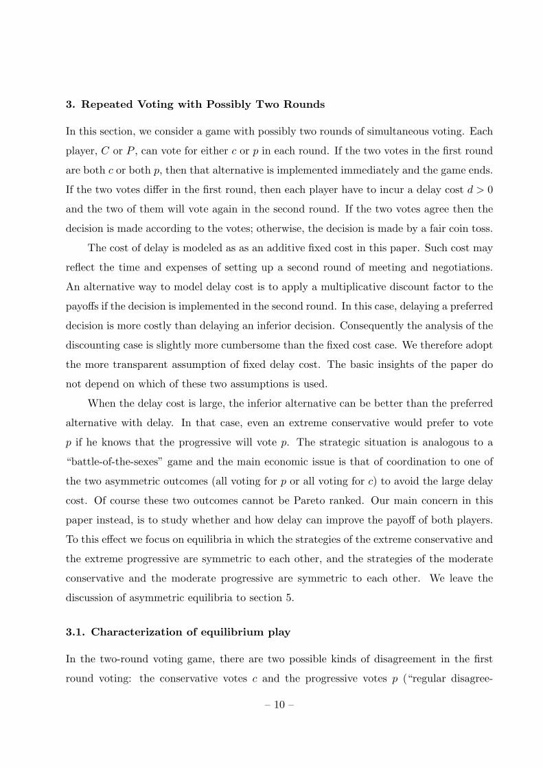
3. Repeated Voting with Possibly Two Rounds

In this section, we consider a game with possibly two rounds of simultaneous voting. Each

player, C or P , can vote for either c or p in each round. If the two votes in the first round

are both c or both p, then that alternative is implemented immediately and the game ends.

If the two votes differ in the first round, then each player have to incur a delay cost d > 0

and the two of them will vote again in the second round. If the two votes agree then the

decision is made according to the votes; otherwise, the decision is made by a fair coin toss.

The cost of delay is modeled as as an additive fixed cost in this paper. Such cost may

reflect the time and expenses of setting up a second round of meeting and negotiations.

An alternative way to model delay cost is to apply a multiplicative discount factor to the

payoffs if the decision is implemented in the second round. In this case, delaying a preferred

decision is more costly than delaying an inferior decision. Consequently the analysis of the

discounting case is slightly more cumbersome than the fixed cost case. We therefore adopt

the more transparent assumption of fixed delay cost. The basic insights of the paper do

not depend on which of these two assumptions is used.

When the delay cost is large, the inferior alternative can be better than the preferred

alternative with delay. In that case, even an extreme conservative would prefer to vote

p if he knows that the progressive will vote p. The strategic situation is analogous to a

“battle-of-the-sexes” game and the main economic issue is that of coordination to one of

the two asymmetric outcomes (all voting for p or all voting for c) to avoid the large delay

cost. Of course these two outcomes cannot be Pareto ranked. Our main concern in this

paper instead, is to study whether and how delay can improve the payoff of both players.

To this effect we focus on equilibria in which the strategies of the extreme conservative and

the extreme progressive are symmetric to each other, and the strategies of the moderate

conservative and the moderate progressive are symmetric to each other. We leave the

discussion of asymmetric equilibria to section 5.

3.1. Characterization of equilibrium play

In the two-round voting game, there are two possible kinds of disagreement in the first

round voting: the conservative votes c and the progressive votes p (“regular disagree-

– 10 –

ment”); and the conservative votes p and the progressive votes c (“reverse disagreement”).

The updating of beliefs of the moderate types upon these two types of disagreement de-

pends on the equilibrium strategies adopted by the players. Suppose in equilibrium the

extreme progressive votes p with probability 1, while the moderate progressive votes p

with probability x1. Then, upon a regular disagreement, the moderate conservative would

revise his belief that the state is M downward to

γ′ =γx1

γx1 + 1− γ≤ γ,

unless γ = 1 and x1 = 0, in which case the Bayes’ formula does not apply. From the

discussion of the previous section, in the final round the extreme types vote according to

their preferences while the equilibrium strategies of the moderate players are given by:

x0(γ′) =

0 if γ′ ∈ [0, 12 ),

∈ [0, 1] if γ′ = 12 ,

1 if γ′ ∈ ( 12 , 1].

Note that γ′ = 12 for any γ ≥ 1

2 if x1 = (1 − γ)/γ, in which case the continuation play is

not unique. Upon a reverse disagreement, the moderate conservative updates his belief to

1, except when x1 = 1, because he can exclude the possibility that the state is L. In the

final round, the moderate players choose x0(1) = 1, and the game ends with the decision

made by a coin flip.

Given this assumed strategy profile, the payoff of the moderate conservative from

voting c is

V c1 (γ, x1) = γ(x1(−d + V0(γ′)) + (1− x1)) + (1− γ)(−d + V0(γ′)), (4)

for all γ and x1 such that γ′ is defined and is not equal to 12 . Let V c

1 (1, 0) = 1,6 and for any

γ ≥ 12 and x1 = (1− γ)/γ, let V c

1 (γ, (1− γ)/γ) represent a continuum of the continuation

payoffs, each of which corresponds to a value of V0( 12 ) ∈ [1−∆, 1− 1

2∆]. The payoff of the

moderate conservative from voting p is

V p1 (γ, x1) = γ[x1(1− 2∆) + (1− x1)(−d + V0(1))] + (1− γ) (5)

6 When the Bayes’ rule does not apply, by construction the choices of the out-of-equilibrium beliefs donot affect the values of V c

1 (1, 0) and V p1 (γ, 1), which are determined by continuity.

– 11 –

for all x1 < 1 with V p1 (γ, 1) = γ(1 − 2∆) + 1 − γ. Let x1(γ) be the x1 that solves

V c1 (γ, x1) = V p

1 (γ, x1), if it exists. We have the following result.7

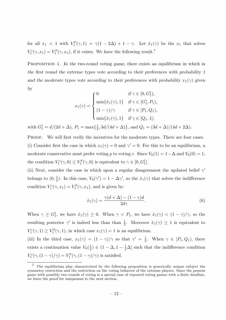
Proposition 1. In the two-round voting game, there exists an equilibrium in which in

the first round the extreme types vote according to their preferences with probability 1

and the moderate types vote according to their preferences with probability x1(γ) given

by

x1(γ) =

0 if γ ∈ [0, G11),

min{x1(γ), 1} if γ ∈ [G11, P1),

(1− γ)/γ if γ ∈ [P1, Q1),

min{x1(γ), 1} if γ ∈ [Q1, 1];

with G11 = d/(2d + ∆), P1 = max{1

2 , 3d/(4d + ∆)}, and Q1 = (3d + ∆)/(4d + 2∆).

Proof. We will first verify the incentives for the moderate types. There are four cases.

(i) Consider first the case in which x1(γ) = 0 and γ′ = 0. For this to be an equilibrium, a

moderate conservative must prefer voting p to voting c. Since V0(1) = 1−∆ and V0(0) = 1,

the condition V c1 (γ, 0) ≤ V p

1 (γ, 0) is equivalent to γ ∈ [0, G11].

(ii) Next, consider the case in which upon a regular disagreement the updated belief γ′

belongs to (0, 12 ). In this case, V0(γ′) = 1−∆γ′, so the x1(γ) that solves the indifference

condition V c1 (γ, x1) = V p

1 (γ, x1), and is given by:

x1(γ) =γ(d + ∆)− (1− γ)d

2dγ. (6)

When γ ≥ G11, we have x1(γ) ≥ 0. When γ < P1, we have x1(γ) < (1 − γ)/γ, so the

resulting posterior γ′ is indeed less than than 12 . Moreover x1(γ) ≥ 1 is equivalent to

V c1 (γ, 1) ≥ V p

1 (γ, 1), in which case x1(γ) = 1 is an equilibrium.

(iii) In the third case, x1(γ) = (1 − γ)/γ so that γ′ = 12 . When γ ∈ [P1, Q1), there

exists a continuation value V0(12 ) ∈ (1 − ∆, 1 − 1

2∆] such that the indifference condition

V c1 (γ, (1− γ)/γ) = V p

1 (γ, (1− γ)/γ) is satisfied.

7 The equilibrium play characterized by the following proposition is generically unique subject thesymmetry restriction and the restriction on the voting behavior of the extreme players. Since the presentgame with possibly two rounds of voting is a special case of repeated voting games with a finite deadline,we leave the proof for uniqueness to the next section.

– 12 –

(iv) When the updated belief γ′ upon a regular disagreement is in ( 12 , 1], we have V0(γ′) =

1−∆. In this case, the solultion x1(γ) to the indifference condition V c1 (γ, x1) = V p

1 (γ, x1)

for the moderate conservative is given by:

x1(γ) =γ(d + ∆)− (1− γ)(d + ∆)

2dγ. (7)

For γ > Q1, we have x1(γ) ≥ (1− γ)/γ, so that γ′ indeed exceeds 12 . Moreover x1(γ) ≥ 1

is equivalent to V c1 (γ, 1) ≥ V p

1 (γ, 1), in which case x1(γ) = 1 is an equilibrium.

To complete the proof, we need to verify that the extreme conservative has no incentive

to deviate to voting p. When the moderate progressive votes p with probability x1, the

extreme conservative’s payoff from voting c is:

W c1 (γ, x1) = x1(−d + W0(γ′)) + (1− x1),

and his payoff from voting p is:

W p1 (γ, x1) = x1(1− 2∆) + (1− x1)(−d + W0(1)).

If x1 = 0, the extreme conservative clearly prefers voting c (with an immediate payoff of

1) to voting p (with a payoff of −d + W0(γ)). If x1 > 0, we have V c1 (γ, x1) ≥ V p

1 (γ, x1), or

γ[x1(−d + V0(γ′)− 1 + 2∆) + (1− x1)(1 + d− V0(1))] + (1− γ)(−d + V0(γ′)− 1) ≥ 0.

The second term of the above expression is strictly negative. Since V0(γ′) ≤ W0(γ′) for all

γ′ and V0(1) = W0(1), the above inequality implies that

x1(−d + W0(γ′)− 1 + 2∆) + (1− x1)(1 + d−W0(1)) > 0,

which is equivalent to W c1 (γ, x1) > W p

1 (γ, x1). Q.E.D.

We say that the moderate conservative “compromises” if he votes c with probability

0. Similarly, the moderate progressive compromises if he votes p with probability 0. In

the one-round voting game, the moderate players compromise if and only if γ < 12 . In the

equilibrium of the two-round voting game, the moderate players compromise in the first

– 13 –

round of voting if and only if γ < G11. Since G1

1 is strictly lower than 12 , the moderate

players are initially less likely to compromise than they are in the benchmark one-round

voting game. More generally, Proposition 1 shows that x1(γ) ≥ x0(γ) for any fixed γ < 12 ,

and the opposite is true for γ > 12 . In other words, introducing the possibility of one more

round of voting tends the make the moderate players tougher in equilibrium if the degree

of conflict is low (γ < 12 ), but it will make the moderate players less tough if the degree of

conflict is high (γ > 12 ). The reason for the different implications to the equilibrium voting

behavior depending on γ, is that delay is unlikely when the degree of conflict is low so the

possibility of re-voting makes the moderate types want to get their own way, while delay

is likely with a high degree of conflict so re-voting makes the moderates more willing to

comprise.

The opportunity of voting again for a second time in case of disagreement also means

that the moderate types can learn from the voting outcome in the first round, even though

no exogenous new information arrives between the two rounds. We may think of learning

in our model as represented by the moderate types’ vote switching between the two rounds.

To this end, it is helpful to classify the different types of equilibrium behavior described

in Proposition 1 according to the first round voting strategy of the moderate players and

how they vote in the second round upon a regular disagreement. When γ ∈ [0, G11), the

moderate players compromise in both rounds.8 We call this a “compromise equilibrium.”

When γ ∈ [G11, P1), the moderate conservative randomizes in the first round but switches

to a compromise vote (i.e., voting p for sure) upon a regular disagreement.9 We call this a

“switching equilibrium.” When γ ∈ [P1, Q1), the moderate conservative randomizes in the

first round. Upon a regular disagreement, his updated belief is γ′ = 12 , so he continues to

randomize in the second round. We call this a “random switching equilibrium.” When γ ∈[Q1, 1], the moderate conservative randomizes in the first round, but never compromises in

8 More precisely, the moderate type is ready to comprise again upon a regular disagreement, whichcan happen only off the equilibrium path.

9 If P1 = 12, or equivalently, if ∆ > 2d, the moderate conservative actually votes c with probability 1

for γ ∈ [d/∆, 12). Upon a regular disagreement, the updated belief stays at γ < 1

2and the moderate types

switch to a comprise in the final round.

– 14 –

0 0.2 0.4 0.6 0.8 10

0.5

1

1.5

2

2.5

3

3.5

4

4.5

5

gamma

Del

ta/d

CompromiseEquilibrium

SwitchingEquilibrium

NoSwitchingEquilibrium

x1=1

x1=1

RandomSwitching

Equilibrium

Figure 1

the next round upon a regular disagreement.10 We call this a “no switching equilibrium.”

Which type of equilibria obtains depends only on γ and ∆/d. Figure 1 summarizes

these results by partitioning the parameter space into four regions with the different types

of equilibria. Note that x1(γ) is not monotone in γ due to the discontinuity in the equi-

librium play x0(γ) in the second round voting at 12 . In a switching equilibrium or a no

switching equilibrium, x1(γ) is increasing in γ, but in a random switching equilibrium, the

value of x1(γ) must be such that the updated belief γ′ is fixed at 12 . In the latter case, the

10 When (d + ∆)/(2∆) < 1, or equivalently, when ∆ > d, the moderate conservative actually votesc with probability 1 for γ ∈ [(d + ∆)/(2∆), 1]. The updated belief upon a regular disagreement stays at

γ > 12

and there is no comprise in the final round. In this case, there is a persistent disagreement betweenthe two players.

– 15 –

higher the γ, the lower must be x1(γ). In this case, the moderate players are less tough

as the degree of conflict increases. However, in spite of the non-monotonicity of x1(γ), the

equilibrium updated belief γ′ is increasing in the prior belief γ, with γ′ being a constant in

[P1, Q1), so that a higher degree of conflict in the first round voting in equilibrium results

a higher degree of conflict in the second round.

The equilibrium value of x1(γ) is weakly increasing in the error cost ∆ and weakly

decreasing in the delay cost d (both within each type of equilibrium and across different

types). In other words, when the delay cost d is low, or when the cost of implementing the

inferior decision ∆ is high, the moderate players will behave in a tougher way by voting

more like extreme players. In the limit, when delay cost d is very small, the equilibrium

outcome in the two-round voting game is a persistent disagreement in both rounds of

voting.

3.2. Welfare analysis

Let V1(γ) denote the expected payoff of the moderate conservative in the two-round voting

game when his belief at the beginning of the first round is given by γ = πM/(πL + πM ).

Similarly, let W1(γ) be the expected payoff of the extreme conservative. The ex ante

welfare of player C is

U1(γ) = (πL + πM )V1(γ) + πRW1(γ) =1

2− γV1(γ) +

1− γ

2− γW1(γ). (8)

We first compare U1 with the equilibrium expected payoff U0 of the one-round voting game

of section 2.

When the degree of conflict between the conservative and the progressive is low, more

specifically, when γ < 12 , a moderate player always yields to his opponent in the one-round

voting game, and the resulting equilibrium is Pareto efficient. Adding the possibility of

another round of voting cannot improve the ex ante welfare of the players. Indeed, it is

easy to show that neither a moderate type nor an extreme type can benefit from having an

additional round of voting. Consider the moderate player first. Suppose x1(γ) < 1. Then

V1(γ) = γ[x1(γ)(1− 2∆) + (1− x1(γ))(−d + V0(1))] + (1− γ)

≤ γ(1−∆) + (1− γ) = V0(γ).

– 16 –

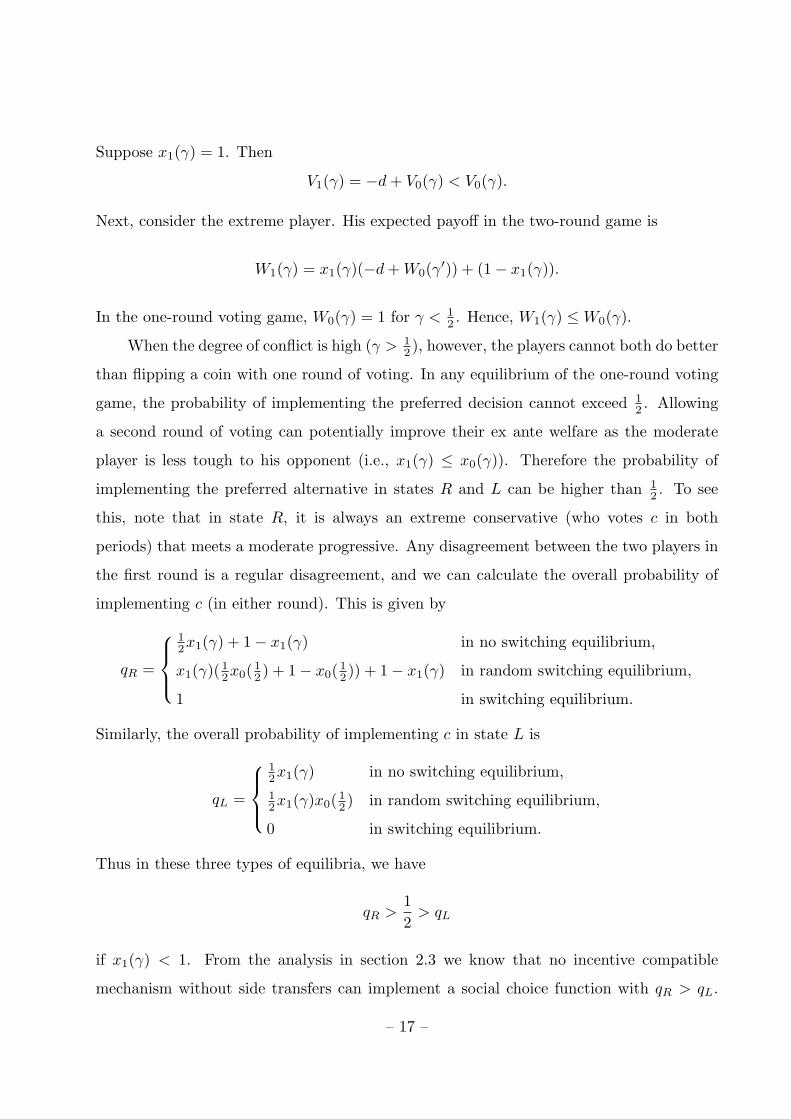
Suppose x1(γ) = 1. Then

V1(γ) = −d + V0(γ) < V0(γ).

Next, consider the extreme player. His expected payoff in the two-round game is

W1(γ) = x1(γ)(−d + W0(γ′)) + (1− x1(γ)).

In the one-round voting game, W0(γ) = 1 for γ < 12 . Hence, W1(γ) ≤ W0(γ).

When the degree of conflict is high (γ > 12 ), however, the players cannot both do better

than flipping a coin with one round of voting. In any equilibrium of the one-round voting

game, the probability of implementing the preferred decision cannot exceed 12 . Allowing

a second round of voting can potentially improve their ex ante welfare as the moderate

player is less tough to his opponent (i.e., x1(γ) ≤ x0(γ)). Therefore the probability of

implementing the preferred alternative in states R and L can be higher than 12 . To see

this, note that in state R, it is always an extreme conservative (who votes c in both

periods) that meets a moderate progressive. Any disagreement between the two players in

the first round is a regular disagreement, and we can calculate the overall probability of

implementing c (in either round). This is given by

qR =

12x1(γ) + 1− x1(γ) in no switching equilibrium,

x1(γ)( 12x0( 1

2 ) + 1− x0( 12 )) + 1− x1(γ) in random switching equilibrium,

1 in switching equilibrium.

Similarly, the overall probability of implementing c in state L is

qL =

12x1(γ) in no switching equilibrium,12x1(γ)x0( 1

2 ) in random switching equilibrium,

0 in switching equilibrium.

Thus in these three types of equilibria, we have

qR >12

> qL

if x1(γ) < 1. From the analysis in section 2.3 we know that no incentive compatible

mechanism without side transfers can implement a social choice function with qR > qL.

– 17 –

This result does not apply to our two-round voting game, because we allow the possibility

that players may have to pay an additional cost d, which is dissipated as delay rather

than transferred to the other player. Thus, it is the possibility of budget breaking that

is responsible for potentially improving the equilibrium outcome.11 Formally, we have the

following proposition.

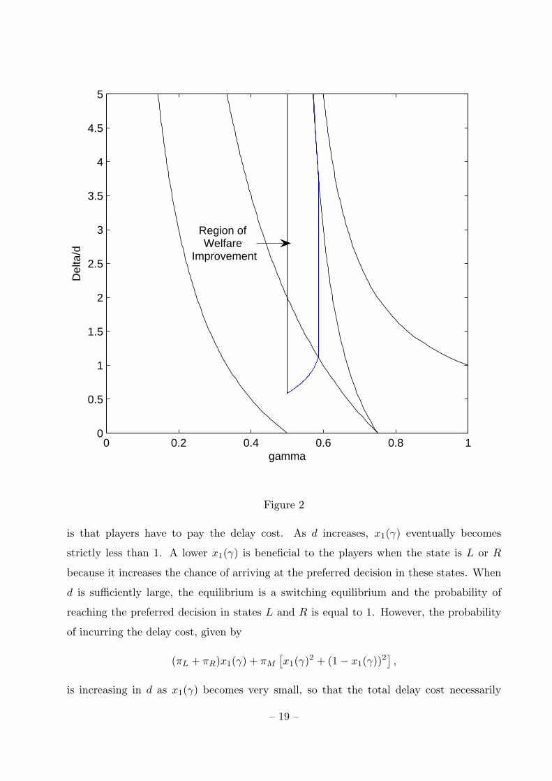
Proposition 2. For each γ ∈ (12 , 2−√2), and only for these values of γ, there exists an

interval of values for ∆/d such that U1(γ) > U0(γ).

The proof of Proposition 2 is in the Appendix, where we give the exact lower bound

and upper on ∆/d as functions of γ such that the ex ante payoff of each player is strictly

higher in an equilibrium of the two-round voting game than in the equilibrium of the

single-round game. Intuitively, welfare gains from introducing the second round of voting

exist only when the degree of conflict is not too high. In particular, when γ is close to 1

so that there is little room for a first-round comprise or subsequent voting switching, the

impact of adding the second round is that the players incur the cost of delay the eventual

disagreement. More generally, Proposition 2 shows that when the degree of conflict is

sufficiently high (γ > 2 − √2), the improvement in the quality of the decision is out-

weighed by the direct cost of delay. Figure 2 provides a graphical depiction of the region

of parameter space for which welfare is higher under the two-round game than under the

benchmark one-round game. Note that this region of welfare improvement contains a

subset of each region in the parameter space corresponding to a no switching equilibrium,

a random switching equilibrium, and a switching equilibrium. In other words, for each of

these three types of equilibria, there are values of γ, ∆, and d such that delay increases

the welfare of each player.

It is clear from Figure 2 that the cost of delay has a non-monotone effect on players’

welfare. Fix γ at some value between 12 and 2−√2. When d is very low, the equilibrium is

a no switching equilibrium with x1(γ) = 1. Since there is complete disagreement between

the players in both rounds, the only effect of introducing an additional round of voting

11 Our idea of using delay as a mechanism to improve collective decision making shares the same logic asin Holmstrom’s (1982) model of moral hazard in teams and Myerson and Satterthwaite model of bilateraltrading with asymmetric information.

– 18 –

0 0.2 0.4 0.6 0.8 10

0.5

1

1.5

2

2.5

3

3.5

4

4.5

5

gamma

Del

ta/d

Region of Welfare

Improvement

Figure 2

is that players have to pay the delay cost. As d increases, x1(γ) eventually becomes

strictly less than 1. A lower x1(γ) is beneficial to the players when the state is L or R

because it increases the chance of arriving at the preferred decision in these states. When

d is sufficiently large, the equilibrium is a switching equilibrium and the probability of

reaching the preferred decision in states L and R is equal to 1. However, the probability

of incurring the delay cost, given by

(πL + πR)x1(γ) + πM

[x1(γ)2 + (1− x1(γ))2

],

is increasing in d as x1(γ) becomes very small, so that the total delay cost necessarily

– 19 –

increases. Beyond a certain point, the direct cost of delay outweighs the benefits from

improving the quality of decisions, and the two-round voting game yields lower ex ante

welfare than the benchmark one round voting game. Nevertheless, Proposition 2 shows

that there is an intermediate range of d such that introducing the possibility of delay will

strictly improve the welfare of the players.

4. Repeated Voting with More than Two Rounds

Consider a repeated voting game with a deadline T ; we allow T to be infinity. By “deadline”

we mean the maximum number of rounds in which the two players can vote again in case

of disagreement. If in any round of voting, the votes of the two players agree, then that

decision is implemented and the payoffs are realized. Each additional round of voting is

associated with an additional delay cost of d to each player. We index the voting rounds

in the reverse order, with the first round being round T , and the final round being round

0. The game considered in section 3 is a special case, with T = 1.

A non-terminal history in this game at some round of voting consists of the first

moves by nature, which determine the permanent type of each player, and subsequent

disagreeing votes cast by the two players. An information set for a player of a given type

is a collection of all histories that begin with the same nature’s move determining the

player’s type and share the same sequence of disagreeing votes. A strategy of a player is

a sequence of randomizations over the two votes for each of his information sets, and a

belief system is a sequence of probability measures over histories for each information set.

A sequential equilibrium is a profile of strategies and a belief system that are sequentially

rational and consistent (Kreps and Wilson, 1982). This seems very complicated, but note

that the only unobserved component of a terminal history that affects the payoff to each

player is the permanent type of his opponent, or equivalently, whether the state is M or

not. We therefore restrict equilibrium strategies of each player such that the vote cast at

all information sets in a given round of voting depends only on his belief that the state is

M , and simultaneously restrict the belief system to the collection of beliefs of each player

at each information set that the state is M . The notions of sequential rationality and

consistency can be applied in a straightforward fashion to the restricted strategy profiles

– 20 –

and belief systems. We refer to the resulting solution concept as “equilibrium.” We look for

equilibria such that in each round of voting on and off the equilibrium path: (i) the extreme

types always vote according to their preferences; and (ii) for each pair of information sets

of the moderate types that share the same sequence of disagreeing votes, the two types

have identical beliefs about the state being M and vote according to their preferences with

the same probability. Note that on the equilibrium path, the notion of consistency in the

definition of sequential equilibrium implies that, if the moderate types vote according to

their preference with the same probability then they have the same belief about the state

being M after any observed sequence of disagreeing votes.

4.1. Repeated voting with a finite deadline

We will establish existence and uniqueness of equilibrium for the game with a finite deadline

T by backward induction. Backward induction is equivalent to mathematical induction on

the deadline T , as a repeated voting game with a finite deadline T and initial belief of the

moderate types that the state is M with probability γ can be alternatively viewed as the

equilibrium continuation game with T + 1 rounds of voting remaining and belief γ for a

game with a longer deadline.

Let t be the number of rounds of voting remaining before the final round, including

the current round; we refer to the current round as round-t voting. Denote as xt(γ) the

common equilibrium probability of the moderate types voting according to their preferences

in a round-t voting when the common belief of the moderate types is that the state is M

with probability γ. Let Vt(γ) and Wt(γ) be the corresponding equilibrium payoffs for

the moderate types and the extreme types. The induction hypothesis is that for any

t = T − 1, . . . , 0 and for any prior belief γ of the moderate types that the state is M ,

in the repeated voting game with a deadline t: (i) there is a unique equilibrium, except

when t < ∆/(2d) and γ = 12 , in which case there is a continuum of equilibria satisfying

xτ ( 12 ) = 1 for all τ = t, . . . , 1; (ii) Vt(γ) is a continuous and piecewise linear function

of γ, except when t < ∆/(2d) and γ = 12 , in which case Vt( 1

2 ) takes any value on the

interval[limγ↓ 1

2Vt(γ), limγ↑ 1

2Vt(γ)

]; and (iii) Vt(1) = Wt(1), and Vt(γ) ≤ Wt(γ) for all γ,

– 21 –

except when t < ∆/(2d) and γ = 12 , in which case Vt( 1

2 ) ≤ Wt( 12 ) for any selection of the

equilibria. Note from equations (1) and (2) the above properties are satisfied for T = 0.

Given the induction hypothesis, we write V ct (γ, xt) as the expected payoff to the

moderate conservative from voting c in round t, when the belief that the state is M is γ

and when the moderate progressive votes p with probability xt. We have:

V ct (γ, xt) = γ(x(−d + Vt−1(γ′)) + (1− xt)) + (1− γ)(−d + Vt−1(γ′)) (9)

for all γ and xt such that γ′ = γxt/(γxt +1−γ) is defined and is not equal to 12 . Next, let

V pt (γ, xt) be the corresponding expected payoff to the moderate conservative from voting

p, given by

V pt (γ, xt) = γ[(xt(1− 2∆) + (1− xt)(−d + Vt−1(1))] + (1− γt) (10)

for any xt < 1. Since Vt−1(γ′) is piecewise linear, we can write it as

Vt−1(γ′) = at−1 − bt−1γ′.

Applying the Bayes’ formula, we have V ct (γ, xt)− V p

t (γ, xt) is given by

γ[xt(−d + at−1 − bt−1 − 1 + 2∆) + (1− xt)(1 + d− Vt−1(1))] + (1− γ)(−d + at−1 − 1).

Note that V ct (γ, xt)− V p

t (γ, xt) is decreasing in xt if

ut−1 ≡ (1 + d− Vt−1(1)) + (1 + d− at−1) + (bt−1 − 2∆) > 0.

Also, if in equilibrium xt ∈ (0, 1) round-t voting, we must have V ct (γ, xt) = V p

t (γ, xt),

which implies

xt =γ(1 + d− Vt−1(1))− (1− γ)(1 + d− at−1)

γut−1.

Substituting this value of xt into V ct (γ, xt) and setting Vt(γ) = at − btγ, we obtain a pair

of difference equations:

at = 1− (1 + d− Vt−1(1)− 2∆)(1 + d− at−1)ut−1

,

bt = 2∆ +(1 + d− Vt−1(1)− 2∆)(bt−1 − 2∆)

ut−1.

(11)

– 22 –

To complete the induction proof for the existence and uniqueness of equilibrium, we

need two preliminary results that can be established by separate induction arguments. For

the first result, let s be the smallest integer that is strictly greater than ∆/d; note that

s ≥ 1. We have:

Lemma 1. (i) For any t ≤ s− 1, in any equilibrium xt(1) = 1 and Vt(1) = 1−∆− td; (ii)

for any t ≥ s, in any equilibrium xt(1) ∈ (0, 1) and Vt(1) satisfies

1− Vt(1) =(1 + d− Vt−1(1))2

2(1 + d− Vt−1(1)−∆);

(iii) Vt(1) > 1− 2∆ for all t ≤ s− 2 and Vt(1) < 1− 2∆ for all t ≥ s− 1; (iv) {Vt(1)} is a

monotonically decreasing sequence, with the limit V∞(1) = 1−∆−√d2 + ∆2.

The proof of Lemma 1 is in the appendix. A key to the proof is that once the

moderates’ belief that the state is M becomes 1, it will remain 1 for the remainder of

the game. This allows to use an induction argument independent of the establishment of

equilibrium existence and uniqueness for the whole game. From the proof we immediately

obtain that xt(1) is strictly decreasing in t for t ≥ s− 1. Thus, in the unique equilibrium

continuation play after a reverse disagreement in the previous round, the moderate types

randomize between the two votes if sufficiently many rounds of voting remain (t ≥ s),

but become tougher as the deadline approaches and eventually revert to voting according

to their preferences.12 Finally, note that since W0(1) = V0(1) and xt(1) > 0 for all t, a

straightforward induction argument establishes that Wt(1) = Vt(1) for all t.

For Lemma 2 below, we study the difference equations (11), using the sequence {Vt(1)}characterized by Lemma 1. From equation (1), there are two sets of initial conditions:

a0 = 1 and b0 = ∆, corresponding to γ < 12 in the final round; and a0 = 1−∆ and b0 = 0,

corresponding to γ > 12 . The proof is in the appendix.

Lemma 2. (i) ut > 0 for all t; (ii) bt ≥ 0 for all t; (iii) at − 12bt < 1−∆ for all t ≥ s; and

(iv) 1 + d− at ≥ 0 for all t ≥ s.

12 Thus, when the deadline is long enough, the equilibrium behavior of the moderate types when γ = 1is different from that of the extreme types, who have the same belief.

– 23 –

Now we are ready to complete the induction argument. Proposition 3 below is the

main characterization result in repeated games with a finite deadline.

Proposition 3. For any finite deadline T , there is a unique equilibrium, except when

T < ∆/(2d) and γ = 12 , in which case there is a continuum of equilibria with xt(1

2 ) = 1

for all t = T, T − 1, . . . , 1.

Proof. First we extend the payoff functions V cT (γ, xT ) and V p

T (γ, xT ), given by equations

(9) and (10) respectively with t = T . Let V cT (1, 0) = 1, and V p

T (γ, 1) = γ(1−2∆)+(1−γ).

For each γ ∈ [ 12 , 1], we let V cT (γ, (1 − γ)/γ) be multi-valued and recursively given by

2(1− γ)(VT−1( 12 )− d) + (2γ − 1).

Next, we claim that the necessary and sufficient conditions for equilibrium in the

repeated game with deadline T are: there is an equilibrium with xT = 0 if and only if

V cT (γ, 0) ≤ V p

T (γ, 0); there is an equilibrium with xT ∈ (0, 1) if and only if V cT (γ, xT ) =

V pT (γ, xT ), or, there exists a value of V c

T (γ, (1 − γ)/γ) equal to V pT (γ, (1 − γ)/γ) in the

case of T < ∆/(2d), γ ∈ [ 12 , 1) and xT = (1 − γ)/γ; and there is an equilibrium with

xT = 1 if and only if V cT (γ, 1) ≥ V p

T (γ, 1). The necessity of the condition for each of the

three cases above is a straightforward application of the one-deviation principle, if the

Bayes’ rule applies. Further, when the Bayes’ rule does not apply, by construction the

choices of the out-of-equilibrium beliefs do not affect the values of V cT (1, 0) and V p

T (γ, 1).

To establish the sufficiency of the conditions, we only need to show that in each case the

extreme conservative does not want to deviate from voting c in round-T voting. This

follows from part (iii) of the induction hypothesis and an identical argument as in the

proof of Proposition 1.

Define DT (γ, xT ) = V cT (γ, xT ) − V p

T (γ, xT ). Then, for any γ, DT is a function of

xT , with the proviso that DT is multi-valued at xT = (1 − γ)/γ for any γ ≥ 12 , as

V cT (γ, (1 − γ)/γ) is multi-valued. We claim that for any fixed γ ∈ [0, 1], DT is a piece-

wise linear, continuous and strictly decreasing function of xT , except at xT = (1 −γ)/γ for T < ∆/(2d) and γ ∈ [ 12 , 1) when DT is multi-valued; DT (γ, (1 − γ)/γ) =[limxT ↓(1−γ)/γ DT (γ, xT ), limxT ↑(1−γ)/γ DT (γ, xT )

]for any γ ∈ ( 1

2 , 1); and DT ( 12 , 1) =[

−d, limxT ↑1 DT ( 12 , xT )

]. Given the definitions of V c

T and V pT , and part (i) and part (ii) of

– 24 –

the induction hypothesis, we only need to show that DT is strictly decreasing in xT except

at xT = (1− γ)/γ for T < ∆/(2d) and γ ∈ [ 12 , 1), which follows from part (i) of Lemma 2.

It follows from the above properties of DT and the equilibrium conditions that: if

DT (γ, 0) ≤ 0, then there is a unique equilibrium with xT = 0; if DT (γ, 0) > 0, and either

DT (γ, 1) < 0 when γ 6= 12 or max DT ( 1

2 , 1) < 0, then there is a unique equilibrium with

xT ∈ (0, 1); if DT (γ, 1) ≥ 0 when γ 6= 12 then there is a unique equilibrium with xT = 1;

and if max DT (12 , 1) > 0, or equivalently if γ = 1

2 and ∆ > 2Td, then there is a continuum

of equilibria with xT = 1, each associated with a value of V0( 12 ) or equivalently a value of

x0( 12 ) satisfying that DT ( 1

2 , 1) ≥ 0. Q.E.D.

The model of repeated voting games with finite deadlines and the above characteri-

zation result allow us to analyze the “deadline effect”: does extending the deadline by one

more round of voting in case of disagreement improve or reduce the ex ante payoff of the

two players? To answer this question, we first note that the deadline effect is negative for

if the degree of conflict as measured by γ is extreme, in the sense that for all finite deadline

T any possibility of re-voting is worse than flipping a coin. At one extreme, for γ = 1,

from Lemma 1 we have WT (1) = VT (1) < V0(1) = W0(1) = 1 −∆ for all finite deadline

T .13 At the other extreme, since the equilibrium outcome in the one-round voting game

(with T = 0) is efficient for γ < 12 , we have VT (γ) < 1 − ∆γ = V0(γ) for the moderate

types while WT (γ) ≤ 1 = W0(γ). Given that the deadline effects are negative for extreme

values of γ , it is natural to consider γ just above 12 . As suggested by Proposition 2, if the

deadline effect is positive, then it is likely to be the most pronounced for γ just above 12 .

For the following proposition, let UT (γ) be the ex ante equilibrium payoff for each player

in the repeated game with deadline T and prior belief of the moderate types that the state

is M with probability γ. Define

QT =(T + 2)d + ∆

2(T + 1)d + 2∆;

13 This is perhaps not surprising, but note that VT (1) and WT (1) decrease with T in spite of the factthat xT (1) weakly decreases with T . That is, despite of softening positions by the moderate types, a longerdeadline only worsens the situation for the two players when the prior level of conflict is sufficiently high.

– 25 –

note that it is strictly greater than 12 and coincides with the value given in Proposition 1

when T = 1.14

Proposition 4. If γ ∈ ( 12 , QT ] and 2 ≤ T < ∆/(2d), then UT (γ) > UT−1(γ).

Proof. Since T − 1 < T < ∆/(2d), by Proposition 3 there is a continuum of equilibria

at γ = 12 in the repeated voting game with deadline T − 1, each of which is associated

with a probability x0( 12 ) of the moderate types voting according to preferences in the final

round. We argue that in the repeated voting game with deadline T , there is an interval

of values of γ, which is given by ( 12 , QT ], such that xT (γ) = (1− γ)/γ, the updated belief

for the moderate types upon a regular disagreement is 12 , and each γ on this interval is

associated with a value of x0(12 ). Given this equilibrium, the expected payoff from voting

c in round T for a moderate conservative with belief γ is:

V cT (γ, (1− γ)/γ) = 2(1− γ)

(− d + VT−1

(12

))+ (2γ − 1)

= 2(1− γ)(− Td + 1− 1

2∆− 1

2x0

(12

)∆

)+ (2γ − 1),

where the second equality follows from induction. The expected payoff from voting p in

round T is

V pT (γ, (1− γ)/γ) = 2(1− γ)(1−∆) + (2γ − 1)(−d + VT−1(1))

= 2(1− γ)(1−∆) + (2γ − 1)(−Td + 1−∆),

where the second equality follows Lemma 1 because T < ∆/(2d) ≤ s − 1. Note that

V pT (γ, (1−γ)/γ) is decreasing in γ, which implies that a greater γ in the interval ( 1

2 , QT ] is

associated with a greater x0( 12 ) and hence a lower value of V0(1

2 ). Solving for x0( 12 ) from

V c(γ, (1− γ)/γ) = V p(γ, (1− γ)/γ) gives

x0

(12

)=

γ

1− γ

Td + ∆∆

− 3Td

∆. (12)

14 For T = 1, we already know from Proposition 2 the necessary and sufficient conditions for U1(γ) >U0(γ). The argument below for Proposition 4 applies intact for the case of T = 1, but when T = 1 and

∆/(2d) arbitrarily close to 1, Q1 is greater than 2 − √2. This is consistent with Figure 2 which showsthat when ∆/(2d) is approaching 1 from above, the region of γ such that U1(γ) > U0(γ) is a sub-interval

of ( 12, Q1].

– 26 –

For γ greater than but arbitrarily close to 12 , we have that x0( 1

2 ) = 1 − 2Td/∆. At

the other end, the upper bound QT of the interval is determined by the largest value of

x0( 12 ), which from the proof of Proposition 3 satisfies V c

T−1(12 , 1) = V p

T−1(12 , 1). This yields

x0( 12 ) = 1 − 2(T − 1)d/∆. Substituting this value of x0( 1

2 ) into equation (12) gives the

largest value of γ for which xT (γ) = (1−γ)/γ. Straightforward calculations show that the

value is QT as defined above.

For any γ ∈ (12 , QT ], the equilibrium payoff to the moderate types in the repeated

voting game with deadline T is given by VT (γ) = V pT (γ, (1−γ)/γ). The equilibrium payoff

to the extreme types is given by

WT (γ) = xT (γ)(− d + WT−1

(12

))+ (1− xT (γ))

=1− γ

γ

(− Td + W0

(12

))+

2γ − 1γ

=1− γ

γ

(− Td + 1− x0

(12

)∆

)+

2γ − 1γ

,

where we have used the fact that xT (γ) = (1− γ)/γ, and that xT−1( 12 ) = . . . = x1( 1

2 ) = 1.

After substituting the expression for x0( 12 ) given in equation (12) into WT (γ) and applying

a version of equation (8) for T , we have for any γ ∈ (12 , QT ],

UT (γ) =1

2− γ(2(1− γ)(1−∆) + (2γ − 1)(−Td + 1−∆))

+1− γ

2− γ

(1− γ

γ(2Td + 1)− (Td + ∆) +

2γ − 1γ

).

(13)

It is straightforward to see that UT (γ) is increasing T if and only if γ < 2−√2. Finally,

given the definition of QT , we can verify that if T ≥ 2 and hence ∆/(2d) > 2, then

QT < 2−√2. Q.E.D.

If we define the “optimal deadline” as the number of re-voting rounds that maximizes

the ex ante welfare of the players, then the above proposition implies that the optimal

deadline is not only positive for intermediate values of γ, as shown in Proposition 2, but

also no smaller than ∆/(2d).15 Thus, if the delay cost d is small, or if the error cost ∆ is

15 For T > ∆/(2d), we can show that for γ just above 12, VT (γ) > V0(γ) if T < ∆/d, but the opposite

is true if T > ∆/d. This follows from the observation that in equilibrium the moderate types randomize

between c and p in round T voting, implying VT (γ) = V pT (γ, xT ) with xT arbitrarily close to xT ( 1

2), and the

characterization of VT−1(1) from part (iii) of Lemma 1. Since WT (γ) ≥ VT (γ) and since W0(γ) = V0(γ),we have UT (γ) > U0(γ). However, we do not know if how UT (γ) compares with UT+1(γ) for T > ∆/(2d).

– 27 –

large, it is likely that extending the deadline by one more round in case of disagreement

is beneficial. Note that from equation (13) in the proof, the ex ante payoff VT (γ) of

the moderate types is decreasing in T , while the payoff WT (γ) to the extreme types is

increasing in T , with the latter dominating in the average payoff UT (γ).

As in the repeated game with possibly two rounds analyzed in section 3, when the

deadline T is relatively short, the discontinuity in the equilibrium play in the final round

generates an interval values of γ on which xT (γ) is decreasing. However, when the deadline

is sufficiently long, we expect the impact of the discontinuity in the final round play

to dissipate, as suggested by Proposition 3 because the equilibrium is unique when the

deadline T exceeds ∆/(2d). In fact, part (iv) of Lemma 2 implies that xT (γ) is increasing

in γ when T ≥ s.16 Since the updated belief γ′ after a regular disagreement satisfies

γ′

1− γ′=

γ

1− γxT (γ) =

γ(1 + d− VT−1(1))− (1− γ)(1 + d− aT−1)(1− γ)uT−1

,

which is increasing in γ, we expect the equilibrium play in repeated voting games with

sufficiently long deadlines to have the feature that in the initial rounds of voting the

moderate types are increasingly more willing to comprise. However, such a conclusion

would require us to argue that xt(γ) changes little if t is sufficiently large. In fact, once

the deadline is near, xt(γ) is no longer monotone even though the updated belief continues

to decrease. Further, Lemma 1 shows that xt(1) is weakly decreasing in t. Since the

updated belief always stays at 1, it is not true that the players are increasingly more

willing to comprise in the initial rounds when they are almost certain that the state is the

disagreement state. In the next subsection we analyze a repeated voting game without

a deadline T in which these reasons for the non-monotonicity of the equilibrium play

disappear.

4.2. Repeated voting without deadline

Consider a game in which players can vote repeatedly for an indefinite number of rounds as

long as they do not agree. We will first construct a stationary equilibrium and then argue

16 Moreover, part (iii) of Lemma 2 states that at − 12bt < 1 − ∆ for all t ≥ s, which implies that

Vt(γ) = at − btγ < 1 − ∆ = V0(γ) for γ > 12, and therefore the moderate types are worse off with any

deadline longer than s compared to a single round of voting.

– 28 –

that it is unique. For each belief γ ∈ [0, 1] that the moderate types hold regarding the

disagreement state M , we denote as x(γ) the equilibrium probability that the moderate

types vote according to their preferences.17 Upon a regular disagreement, the moderate

players’ belief that the state is M is revised downward to

γ′ =γx(γ)

γx(γ) + 1− γ,

if it is not the case that γ = 1 and x(1) = 0. Upon a reverse disagreement, on the other

hand, the moderates are sure that his opponent is a moderate and therefore his belief that

the state is M jumps to 1, unless x(γ) = 1.

As in the case of finite deadlines, we construct an equilibrium by first considering the

equilibrium play when the moderate players believe that the state is M with probability

1. It is straightforward to see that in any equilibrium x(1) ∈ (0, 1). If the moderate

progressive votes p with probability 1, then for the moderate conservative the outcome

from voting c would be delay forever, which is strictly worse than conceding by voting p;

and if the moderate progressive votes c with probability 1, then voting c would bring an

immediate agreement and strictly dominate voting p. Neither case can be an equilibrium.

It then follows from the indifference condition that

V (1) = x(1)(−d + V (1)) + (1− x(1)) = x(1)(1− 2∆) + (1− x(1))(−d + V (1)).

Solving these two equations gives a unique pair of equilibrium values

V (1) = 1−∆−√

d2 + ∆2,

x(1) =−d + ∆ +

√d2 + ∆2

2∆.

(14)

We note that V (1) < 1− 2∆, and it is the same value identified in part (iv) of Lemma 1,

where we have used the different notation of V∞(1).

Next, consider the equilibrium play when γ = 0. Since the moderate conservative

believes that the state is L and his opponent (who is an extreme progressive) votes p,

voting p to obtain the preferred decision is strictly better than voting c. Thus, we have

17 For notational brevity, we will drop the subscripts ∞ from all variables.

– 29 –

x(0) = 0 and V (0) = 1. Given this, when γ is positive but sufficiently small the moderate

players vote against their preferences with probability 1. To see this, note that x(γ) = 0

implies that the updated belief upon a regular disagreement is γ′ = 0. Therefore, the

payoff to a moderate conservative from voting c is

V c(γ, 0) = γ + (1− γ)(−d + V (0)),

and his payoff from voting p is

V p(γ, 0) = γ(−d + V (1)) + (1− γ).

Voting p is strictly preferred to voting c if and only if

γ <d

(1 + d− V (1)) + d≡ G1.

Therefore, when γ < G1, in equilibrium the moderate conservative votes p and his corre-

sponding equilibrium payoff takes the linear form of

V (γ) = 1− (1 + d− V (1))γ. (15)

Conversely, when γ > G1, in any equilibrium we have x(γ) > 0.

We refer to the interval [0, G1] as the “compromise region.” For γ just above G1, it

is natural to conjecture that the equilibrium x(γ) is such that the one-step updated belief

γ′ falls into the compromise region. We may then try to identify some one-step interval

[G1, G2], and so on. This conjecture turns out to be correct. That is, there exists an

infinite sequence, G0 < G1 < G2 < . . ., with G0 = 0 and limk→1 Gk = 1, such that if

γ ∈ (Gk, Gk+1] for k = 1, 2, . . ., then x(γ) is such that γ′ = γx(γ)/(γx(γ) + 1 − γ) ∈(Gk−1, Gk]. Furthermore, we conjecture that the value function is piecewise linear of the

form V (γ) = ak− bkγ for γ ∈ (Gk, Gk+1], with a0 = 1 and b0 = 1+d−V (1) from equation

(15). Let γ ∈ (Gk, Gk+1] for k ≥ 1. Given the conjecture, the expected payoff to the

moderate conservative from voting c is

V c(γ, x) = (γx + 1− γ)(−d + ak−1 − bk−1γ′) + γ(1− x)

= (γx + 1− γ)(−d + ak−1)− γxbk−1 + γ(1− x).

– 30 –

The payoff from voting p is

V p(γ, x) = γ[x(1− 2∆) + (1− x)(−d + V (1))] + (1− γ).

The moderate conservative is indifferent between voting c and voting p when x is given by

x(γ) =γ(1 + d− V (1))− (1− γ)(1 + d− ak−1)

γ((1 + d− V (1)) + (1 + d− ak−1) + (bk−1 − 2∆)). (16)

Substituting the above into the expression for V c, we obtain V (γ) = ak − bkγ, where

ak = 1− (1 + d− ak−1)(b0 − 2∆)b0 + (1 + d− ak−1) + (bk−1 − 2∆)

,

bk = 2∆ +(b0 − 2∆)(bk−1 − 2∆)

b0 + (1 + d− ak−1) + (bk−1 − 2∆).

(17)

Equation (17) is a pair of difference equations for the sequence {(ak, bk)}. We have the

following preliminary result regarding (17).

Lemma 3. (i) ak ≤ 1 and bk > 2∆ for all k; (ii) both ak and bk are decreasing in k; and

(iii) limk→∞ ak = 1 + ∆−√d2 + ∆2 and limk→∞ bk = 2∆.

The proof of the lemma is in the appendix. Note that by part (ii) of the lemma, the

implied value function V (γ) for the moderate types is convex. We are now ready to state

our main result.

Proposition 5. There exists an infinite sequence, G0 < G1 < G2 < . . ., with G0 = 0 and

limk→1 Gk = 1, such that if γ ∈ [G0, G1], then x(γ) = 0; if γ ∈ (Gk, Gk+1] for k = 1, 2, . . .,

then x(γ) satisfies γx(γ)/(γx(γ) + 1− γ) ∈ (Gk−1, Gk].

Proof. Starting with G1 = d/(b0 + d), we define G2, G3, . . ., recursively using the

relation:Gk+1x(Gk+1)

Gk+1x(Gk+1) + 1−Gk+1= Gk.

Using the equilibrium x(·) function given by equation (16), the above can be rewritten as:

Gk+1 =(1 + d− ak−1) + Gk(b0 + bk−1 − 2∆)b0 + (1 + d− ak−1) + Gk(bk−1 − 2∆)

. (18)

– 31 –

We note that G1 is strictly between 0 and 1. Since ak−1 ≤ 1 and bk−1 > 2∆, an induction

argument establishes that Gk ∈ (0, 1) for all k ≥ 1. Furthermore, subtracting Gk from

both sides of (18), we obtain

Gk+1 −Gk =(1 + d− ak−1)(1−Gk) + (bk−1 − 2∆)Gk

(1 + d− ak−1) + b0 + (bk−1 − 2∆)Gk> 0.

Since Gk is an increasing and bounded sequence, it has a limit value, which is found to be

equal to 1.

Fix any γ ∈ (Gk, Gk+1]. By the Bayes’ rule, we have

γ′

1− γ′=

γ

1− γx(γ),

where x(γ) is given by (16). It follows that that γ′ is increasing in γ. Since the sequence

{Gk} is defined in such a way that γ′ = Gk if γ = Gk+1 and γ′ = Gk−1 if γ = Gk, for any

γ ∈ (Gk, Gk+1] we must have γ′ ∈ (Gk−1, Gk].

Lastly, we verify that the extreme types have no incentive to deviate by voting against

his preferences. To this end, let W (γ) be the value function of the extreme conservative

when the moderate type is having belief γ that the state is M . For γ ∈ [G0, G1], since

his opponent is choosing x(γ) = 0, the extreme conservative’s payoff from voting c is 1,

while his payoff from voting p is −d + W (1) < 1. Therefore, the extreme conservative

indeed votes c, implying that W (γ) = 1 > V (γ). For γ = 1, since his opponent is

choosing p with probability x(1), the extreme conservative is indifferent between voting

c and voting p, and his payoff is W (1) = V (1). Finally, for γ ∈ (Gk, Gk+1], k = 1, . . .,

since the moderate conservative is randomizing between voting c and voting p, we have

V c(γ, x(γ)) = V p(γ, x(γ)). This indifference condition can be written as

γ [x(γ)(−d + V (γ′)− 1 + 2∆) + (1− x(γ))(1 + d− V (1))] + (1− γ)(−d + V (γ′)− 1) = 0,

where γ′ = γx(γ)/(γx(γ) + 1 − γ) ∈ (Gk−1, Gk]. Since the last term is strictly negative,

this above inequality implies that the expression in the square bracket is strictly positive.

Note that we have already shown W (1) = V (1). Thus, if W (γ′) > V (γ′), then

x(γ)(−d + W (γ′)− 1 + 2∆) + (1− x(γ))(1 + d−W (1)) > 0,

– 32 –

which is equivalent to the condition that the extreme conservative strictly prefers voting

c to voting p. That W (γ) > V (γ) for all γ < 1 can be established by induction, as

follows. We already know W (γ) = 1 > V (γ) for γ ∈ [G0, G1]. For any γ ∈ [Gk, Gk+1] and

k = 1, . . ., with γ′ = γx(γ)/(γx(γ) + 1− γ) ∈ (Gk−1, Gk], we have

W (γ) > (γx(γ) + 1− γ)(−d + W (γ′)) + γ(1− x(γ))

> (γx(γ) + 1− γ)(−d + V (γ′)) + γ(1− x(γ))

= V (γ),

where the first inequality follows from the fact that x(γ) < γx(γ) + 1− γ and the second

inequality follows from the induction hypothesis. Q.E.D.

The equilibrium stated in Proposition 5 can be described easily. In each round of

voting, there are four possible outcomes: immediate agreement on c, immediate agreement

on p, a regular disagreement, or a reverse disagreement. We interpret a reverse disagree-

ment as a breakdown of the negotiation process. Once a reverse disagreement occurs, it

is revealed that what is a good decision for one player is necessarily an inferior decision

for another player. The voting game then evolves just like an battle-of-the-sexes game

with attrition, in which each moderate player chooses the stationary strategy represented

by x(1) until they reach a decision. Upon a regular disagreement, on the other hand, the

moderate player is more convinced that he is playing against an extreme type. The ex-

treme type will continue to vote according to his preference, but the moderate player will

soften his position as x(γ′) < x(γ). In a sense, the negotiation between the two players is

making progress, because the probability of choosing the mutually preferred decision rises

if the state is L or R. Moreover, for any γ bounded away from 1, it only takes a finite

number of rounds of regular disagreement before the moderate player yields to his oppo-

nent completely by switching to vote against his his preference (i.e., x(γ) = 0), provided

there is no breakdown of negotiation before that. Once the game reaches this stage, there

is either agreement on the mutually preferred decision, or the negotiation breaks down and

the two moderate players engage in a war of attrition by adopting the strategy of voting

according to his preference with probability x(1).

– 33 –

The equilibrium constructed in Proposition 5 is unique subject to a weak continuity

restriction. More specifically, the function x(γ) given in the proposition is the unique

continuous function that gives the equilibrium probability of voting according their pref-

erences by the moderate types for each γ ∈ [0, 1]. To see this, first we argue that in any

equilibrium the moderate types must vote against their preferences with probability 1 if

their belief γ is in [0, G1]. To see this, note that regardless of the continuation plays,

V c(γ, x) < V p(γ, x) for all x if γ is sufficiently small, implying that in any equilibrium

x(γ) = 0 for γ sufficiently small, while V c(γ, 1) < V p(γ, 1) for γ < G1, implying that

in any equilibrium x(γ) is bounded away from 1. Then, if it is not true that x(γ) = 0

for all γ ∈ [0, G1], there would be some γ ∈ (0, G1] such that the equilibrium play of the

moderate types is given by x ∈ (0, 1) followed by the moderate types voting against their

preferences with probability 1 upon a regular disagreement, which makes it impossible to

satisfy the indifference condition V c(γ, x) = V p(γ, x). Next, fix any k ≥ 1 and consider

the interval (Gk, Gk+1]. For any γ on this interval such that the equilibrium probability x

of voting according to their preferences satisfies that the updated belief γ′ upon a regular

disagreement γx/(γx+1−γ) is smaller than or equal to Gk, by induction there is a unique

continuation value V (γ′) as given by the proposition. Thus, we must have x = x(γ), be-

cause for each γ′ ≤ Gk and the corresponding k′ ≤ k−1, only x(γ) simultaneously satisfies

the equilibrium condition of V c(γ, x) = V p(γ, x) and the Bayes’ rule γ′ = x/(γx + 1− γ).

Finally, we can rule out by contradiction the possibility that there is a subset of (Gk, Gk+1]

of a positive measure such that for each γ on this subset the equilibrium x is such that the

updated belief γ′ is greater than Gk. By the restriction of continuity of x as a function of

γ, the infimum of this subset γ also has the property that the corresponding equilibrium x

is such that the updated belief γ′ is greater than or equal to Gk. Clearly, x < 1; otherwise,

we would have V (γ) = V (γ) − d, which is impossible. It then follows that Gk ≤ γ′ < γ,

which contradicts the continuity restriction at γ since we have already shown that for any

γ ∈ [Gk, γ) the equilibrium play is given by x(γ) defined in Proposition 5.

We can also show that the equilibrium constructed in Proposition 5 is the limit of

the equilibria established in Proposition 3 as the deadline T becomes arbitrarily large. To

see this, first note that by Proposition 3, when T is sufficiently large, there is a unique

– 34 –

equilibrium. Next, from Lemma 1 we have that xT (1) < 1, and since {VT (1)} converges to

V (1), the sequence {xT (1)} converges to x(1) given in (14). At the other end, the comprise

region for a finite deadline T is determined by

V cT (γ, 0)− V p

T (γ, 0) = γ + (1− γ)(VT−1(0)− d)− (γ(VT−1(1)− d) + (1− γ)),

where VT−1(0) = 1 following from a straightforward induction argument that xt(0) = 0

for all t. We have xT (γ) = 0 for all γ such that V cT (γ, 0) ≤ V p

T (γ, 0), or

γ ≤ d

1 + 2d− VT−1(1)≡ G1

T .

Since VT−1(1) is arbitrarily close to V (1), we have G1T converging to G1 as T converges to

infinity. A straightforward induction argument then shows that for each k = 1, . . ., when

T is sufficiently large, we can define Gk+1T and xT (γ) for any γ ∈ (Gk

T , Gk+1T ], such that

limT→∞Gk+1T = Gk+1 and xT (γ) = x(γ), establishing convergence.

Due to the stationarity of the equilibrium strategy, comparative statics analysis is

cleaner and more intuitive when there is no deadline. The following proposition establishes

as the delay cost increases, or equivalently, as the error cost ∆ decreases, equilibrium voting

by the moderate types becomes less tough for any degree of conflict except for when they are

certain what the state is. In spite of the softening of positions, however, the moderate types

are unambiguously worse off because the direct impact of a greater delay cost dominates.

Proposition 6. As d increases, Gk strictly increases for each k ≥ 1, and V (γ) and x(γ)

strictly decrease for all γ ∈ (0, 1).

The proof the above result is in the appendix. As in the game with T = 1 in section

3, the overall impact of an increase in the delay cost d turns out to be non-monotone.

The reason is that the effect on the payoffs of the extremes is non-monotone. For any

γ ∈ [Gk, Gk+1], k = 0, 1, . . ., the equilibrium payoff W (γ) to the extreme types can be

written as

1− (x(γk) + x(γk)x(γk−1) + . . .)d,

where γk = γ, and for each l = k − 1, . . . , 1,

γl =γl+1x(γl+1)

γl+1x(γl+1) + 1− γl+1

– 35 –

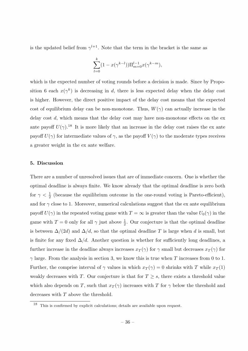
is the updated belief from γl+1. Note that the term in the bracket is the same as

k∑

l=0

(1− x(γk−l))Πl−1m=0x(γk−m),

which is the expected number of voting rounds before a decision is made. Since by Propo-

sition 6 each x(γk) is decreasing in d, there is less expected delay when the delay cost

is higher. However, the direct positive impact of the delay cost means that the expected

cost of equilibrium delay can be non-monotone. Thus, W (γ) can actually increase in the

delay cost d, which means that the delay cost may have non-monotone effects on the ex

ante payoff U(γ).18 It is more likely that an increase in the delay cost raises the ex ante

payoff U(γ) for intermediate values of γ, as the payoff V (γ) to the moderate types receives

a greater weight in the ex ante welfare.

5. Discussion

There are a number of unresolved issues that are of immediate concern. One is whether the

optimal deadline is always finite. We know already that the optimal deadline is zero both

for γ < 12 (because the equilibrium outcome in the one-round voting is Pareto-efficient),

and for γ close to 1. Moreover, numerical calculations suggest that the ex ante equilibrium

payoff U(γ) in the repeated voting game with T = ∞ is greater than the value U0(γ) in the

game with T = 0 only for all γ just above 12 . Our conjecture is that the optimal deadline

is between ∆/(2d) and ∆/d, so that the optimal deadline T is large when d is small, but

is finite for any fixed ∆/d. Another question is whether for sufficiently long deadlines, a

further increase in the deadline always increases xT (γ) for γ small but decreases xT (γ) for

γ large. From the analysis in section 3, we know this is true when T increases from 0 to 1.

Further, the comprise interval of γ values in which xT (γ) = 0 shrinks with T while xT (1)

weakly decreases with T . Our conjecture is that for T ≥ s, there exists a threshold value

which also depends on T , such that xT (γ) increases with T for γ below the threshold and

decreases with T above the threshold.

18 This is confirmed by explicit calculations; details are available upon request.

– 36 –

Below we briefly discuss two perhaps less immediate, but not less interesting, issues

that arise in the two-round voting model of section 3. We have done some work on the

issues but plan to investigate them further.

5.1. Asymmetric equilibria

The four types of equilibria describe in section 3 do not exhaust all possible equilibria

of the two-round voting game. Unlike the single-round voting game analyzed in section

2.2, which generically has no asymmetric equilibria because each type has a dominant

strategy, the possibility of re-voting allows the two players to coordinate by having one

of them play tougher than the other in the first round and then switch the roles in the

second round. As a result, asymmetric equilibria generally exist alongside the symmetric

equilibria identified in Proposition 1. Here, we give a catalog and a brief discussion of all the

possible asymmetric equilibria that can exist. Throughout the discussion, we assume that

player P plays tougher than C in the first round; for each type of asymmetric equilibrium

constructed below, there is another one in which the roles of the two players are switched.

The first type of asymmetric equilibrium can be called a “yielding equilibrium.” Sup-

pose both the moderate and extreme progressive vote p in round one. Then, when the

delay cost is sufficiently large, it can be a best response for the moderate conservative to

yield by voting p as a pure strategy. In terms of our notation in section 2.2, xP = 1 and

xC = 0 in a yielding equilibrium. To have this as an equilibrium, first we need d > 2∆;

otherwise, the extreme conservative would prefer to vote p as well in the first round, as

the payoff from voting p is 1− 2∆ and the payoff from c is −d + 1. (The incentive for the

extreme progressive is satisfied as he gets the maximum payoff of 1 by voting p.) Second,

we need γ > d/(2d + ∆) (which is equal to G11), in order for the moderate progressive to

prefer p to c, or

γ + (1− γ)(−d + 1) > γ(1− d−∆) + (1− γ).

Third, to figure out the incentive of the moderate conservative, we need to consider two

cases of what happens when he deviates and votes c in the first round: if γ > 12 , the

optimal continuation play is vote c, because the moderate progressive will switch to c in

– 37 –

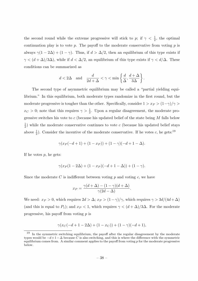
the second round while the extreme progressive will stick to p; if γ < 12 , the optimal

continuation play is to vote p. The payoff to the moderate conservative from voting p is

always γ(1 − 2∆) + (1 − γ). Thus, if d > ∆/2, then an equilibrium of this type exists if

γ < (d + ∆)/3∆), while if d < ∆/2, an equilibrium of this type exists if γ < d/∆. These

conditions can be summarized as

d < 2∆ andd

2d + ∆< γ < min

{d

∆,d + ∆3∆

}.

The second type of asymmetric equilibrium may be called a “partial yielding equi-

librium.” In this equilibrium, both moderate types randomize in the first round, but the

moderate progressive is tougher than the other. Specifically, consider 1 > xP > (1−γ)/γ >

xC > 0; note that this requires γ > 12 . Upon a regular disagreement, the moderate pro-

gressive switches his vote to c (because his updated belief of the state being M falls below12 ) while the moderate conservative continues to vote c (because his updated belief stays

above 12 ). Consider the incentive of the moderate conservative. If he votes c, he gets:19

γ(xP (−d + 1) + (1− xP )) + (1− γ)(−d + 1−∆).

If he votes p, he gets:

γ(xP (1− 2∆) + (1− xP )(−d + 1−∆)) + (1− γ).

Since the moderate C is indifferent between voting p and voting c, we have

xP =γ(d + ∆)− (1− γ)(d + ∆)

γ(2d−∆).

We need: xP > 0, which requires 2d > ∆; xP > (1−γ)/γ, which requires γ > 3d/(4d+∆)

(and this is equal to P1); and xP < 1, which requires γ < (d + ∆)/3∆. For the moderate

progressive, his payoff from voting p is

γ(xC(−d + 1− 2∆) + (1− xC)) + (1− γ)(−d + 1),

19 In the symmetric switching equilibrium, the payoff after the regular disagreement by the moderatetypes would be −d+1−∆ because C is also switching, and this is where the difference with the symmetricequilibrium comes from. A similar comment applies to the payoff from voting p for the moderate progressivebelow.

– 38 –

while his payoff from voting c is

γ(xC(1− 2∆) + (1− xC)(−d + 1−∆)) + (1− γ).

Indifference requires

xC =γ(d + ∆)− (1− γ)d

γ(2d + ∆).

We want to make sure: xC > 0, which requires γ > d/(2d + ∆) and is satisfied because

γ > 12 ; and xC < (1− γ)/γ, which requires γ < (3d + ∆)/(4d + 2∆) (and this is equal to

Q1). These conditions can be summarized as

2d > ∆ and3d

4d + ∆< γ < min

{d + ∆3∆

,3d + ∆4d + 2∆

}.

The third possible type of asymmetric equilibrium is a “random yielding equilibrium.”

In this type of equilibrium, xP = 1 and xC = (1 − γ)/γ (which again requires γ > 12 ).

Upon a regular disagreement, the moderate progressive randomizes in the second round,

voting p with probability x0 ∈ [0, 1], while the moderate conservative continues to vote c

because his belief is unchanged. The payoff to the moderate conservative from voting c in

the first round is

γ(−d + x0(1−∆) + (1− x0)) + (1− γ)(−d + 1−∆),

and his payoff from voting p is γ(1− 2∆) + (1− γ). For the moderate conservative to be

indifferent between the two votes, with x0 varying from 0 to 1, we need

γ(∆− d) < (1− γ)(d + ∆) < γ(2∆− d),

which is satisfied if and only if d < 2∆, γ > (d + ∆)/∆ and γ < min{(d + ∆)/(2∆), 1}.For the moderate progressive, the payoff from voting c in the first round is

γ(xC(1− 2∆) + (1− xC)(−d + 1−∆)) + (1− γ),

while the payoff from voting p is

γ(xC(−d+x0(1−∆)+(1−x0)(1− 2∆))+ (1−xC))+ (1− γ)(−d+x0(1−∆)+(1−x0)).

– 39 –

Substituting xC = (1 − γ)/γ into the above two expressions and comparing them, we

have that the moderate progressive prefers p to c if and only if γ > (3d + ∆)/(4d + ∆).

Summarizing, the necessary and sufficient conditions for this type of equilibria are

d < 2∆ and max{

d + ∆3∆

,3d + ∆4d + 2∆

}< γ < min

{d + ∆2∆

, 1}

.

Since our game in section 3 is symmetric, an asymmetric equilibrium exists only with

one-sided vote-switching in the second round after a regular disagreement by the two

moderate types in the first round. It follows that the above are the only three types of

asymmetric equilibria that exist generically.20 We have yet to investigate whether a simple

average of asymmetric equilibrium plays always improves on the symmetric equilibrium

outcome we have constructed. Our conjecture is that any welfare improvement arises

because asymmetric plays avoid the costly simultaneous vote-switching after a regular dis-

agreement that occurs in a symmetric switching equilibrium. Another way to understand

any potential welfare improvement is that asymmetric plays allow players to trade votes

inter-temporally, and thus circumvent the constraint of no side transfers in our model.

This then appears to be another mechanism for delay to improve strategic information ag-

gregation, different from the one identified in symmetric equilibrium plays in which delay

improves welfare by breaking the “incentive budget.” Finally, any asymmetric play still

requires at least some coordination such as pre-play public randomizations. Whether such

coordination is realistic in applications is an issue that needs to be addressed.

5.2. Optimal delay mechanism

We have presented the idea that delay can be used as a mechanism to improve collective

decision making. As shown in section 2.3, without delay there is no incentive compatible

outcome that beats flipping a coin when γ is greater than 12 , while Proposition 2 shows

that with delay there can be Pareto improving equilibrium outcome for γ just above 12 . A

20 The fourth candidate for asymmetric equilibria, which is given by xP = (1− γ)/γ and xC = 0 withrandom one-sided switching, does not exist generically. This is because only off the equilibrium path canthe moderate conservative randomize in the second round after a regular disagreement in the first round.The indifference condition for the moderate progressive cannot be satisfied generically.

– 40 –

natural question is whether there are other mechanisms using delay that are even better

for the players. This question bears resemblance to the problem of “dynamic mechanism

design” in the existing literature (Dewatripont 1988; Laffont and Tirole 1988). Although

unlike the existing models in the present setup we do not allow side transfers, it is still

useful to relate to the literature in the three different commitment environments that have

been used. Note that in discussing the different commitment environments, we implicitly

assume that the two players have full commitment power regarding the implementation

the pre-specified decision before delay and the imposition of delay; it is only whether or

not they have any commitment power regarding how the decision is made after delay that

differentiates the three commitment environments.21 For the discussion in this subsection,

we assume that γ > 12 .

Under full commitment, the two players can adopt any direct mechanism that maps

two reports of the signals to a probability of choosing c without delay, a probability of

choosing p without delay, and the remaining probability of imposing the delay cost on

each player and getting a continuation outcome. Under full commitment, the continuation

outcome associated with any pair of reports can be an arbitrary mixture between c and p.

Since each player only cares about the total probability that each alternative is chosen and

the probability of paying the delay cost, the revelation principle allows us to represent any

delay mechanism by pairs of the total probability that a particular alternative is chosen

and the probability of delay. As in section 2.3, we denote as qR, qM , and qL the total

probabilities of implementing alternative c when the inferred true state is R, M , and L,

respectively, and denote as q the total probability of implementing c when the reports

are inconsistent. Let the corresponding probabilities of delay be ηR, ηM , ηL and η. For

simplicity, we restrict our attention to symmetric mechanisms, with qR = 1 − qL = q,

qM = q = 12 , and ηR = ηL = η. The incentive constraint for truthful reporting is

q + (1− q)(1− 2∆)− ηd ≥ 1−∆− ηMd

21 There is also a literature on renegotiation in “static” mechanism design problems, where the issueis whether or not there is any commitment regarding implementation of the specified outcome after themechanism is played (i.e., at the ex post stage), or regarding the play of the mechanism itself before themechanism is played (i.e., at the interim stage). See Maskin and Moore (1999), and Segal and Whinston(2002) for renegotiation under complete information, and Holmstrom and Myerson (1983) under incompleteinformation.

– 41 –

for the extremists, and

γ(1−∆− ηMd) + (1− γ)(q + (1− q)(1− 2∆)− ηd)

≥ γ(q + (1− q)(1− 2∆)− ηd) + (1− γ)(1−∆− ηd)

for the moderate types. The objective for this design problem is to maximize U(γ), where

V (γ) and W (γ) are given by the left-hand-side of the above incentive constraint for the

moderates and for the extremists, respectively. It is straightforward to see that the first

best is achieved with q = 1, η = ηM = 0 and η = 1, if and only if γ ≤ (d + ∆)/(d +2∆). If

γ > (d+∆)/(d+2∆), in any optimal mechanism, the incentive constraint for the moderates

binds, with ηM = 0 and η = 1, and q and η satisfying

q + (1− q)(1− 2∆)− ηd = 1−∆ +1− γ

2γ − 1d. (19)

Thus, the same optimal value for U(γ) can be achieved by delay mechanisms that involve

either delay when the state inferred from the reports is an agreement state R or L, or a

probability of implementing the agreement that is strictly less than 1, or both. Moreover,

this value is strictly increasing in the delay cost d until the first best is achieved. Finally,

there is always an optimal delay mechanism with η = 0: since the right-hand-side of (19)

reaches the minimum of 1−∆ when γ = 1, in which case (19) is satisfied with q = 12 and

η = 0, if for some γ < 1 there exist q and η > 0 such that (19) holds, then there exists

q ∈ (12 , q) such that (19) holds with q and η = 0. Thus, an optimal delay mechanism may

not involve delay on the equilibrium path at all.

A commitment environment that is less stringent, and perhaps more realistic, referred

to as “commitment through renegotiation” in the literature (Dewatripont 1988), leads to

the following mechanism design problem in our setup. As in the case of full commitment,

each mechanism under consideration consists of a message space for each player, corre-

sponding to the two possible private signals they can have, and an outcome function that

maps each pair of reports to a probability of choosing c without delay, a probability of

choosing p without delay, and the remaining probability of imposing the delay cost on each

player and getting a continuation outcome. Unlike in the case of full commitment, where

each continuation outcome can be an arbitrary randomization between the two alterna-

tives, here on the truth-telling equilibrium path it has to be renegotiation-proof, which

– 42 –

translates into a requirement that the two players choose the mutually preferred alterna-

tive if it exists. Using the same notation as in the full commitment environment analyzed

above, and again restricting to symmetric mechanisms, we can write one implication of

the renegotiation-proof constraint as q ≥ η. For example, when the state is R, following

any delay the continuation probability choosing c will be renegotiated to 1, and therefore

the total probability of choosing c is greater than or equal to the probability that delay

occurs. Another implication of renegotiation-proofness is more subtle: players must not

benefit by deviating and anticipating the renegotiation after inconsistent reports.22 For

example, the two reports are inconsistent when the moderate conservative misreports his

type and when the other player is an extreme progressive reporting truthfully. In this case,

the continuation outcome after delay will be renegotiated to choosing p with probability 1,

as the progressive knows the state is L. Thus, the truth-telling condition for the moderates

becomes:

γ(1−∆− ηMd) + (1− γ)(q + (1− q)(1− 2∆)− ηd)

≥ γ(q + (1− q)(1− 2∆)− ηd) + (1− γ)((1− η)(1−∆) + η(1− d)).

The strongest incentive for truthful reporting is therefore provided by either η = 0 if

∆ ≥ d, or η = 1 if ∆ < d. In the former case, it follows from the two incentive constraints

for truth-telling that any optimal renegotiation-proof mechanism must have ηM = 0 and

η = 12 , implying that the optimal mechanism is equivalent to flipping a coin. In the

latter case, it is straightforward to show that the first best can be achieved if and only if

γ ≤ d/(d+∆), which is smaller than the threshold (d+∆)/(d+2∆) under full commitment.

If γ > d/(d + ∆), in any optimal mechanism ηM = 0, and q and η satisfy

q + (1− q)(1− 2∆)− ηd = 1−∆ +1− γ

2γ − 1(d−∆).

As in the case of full commitment, if the above is satisfied by some q and η > 0, there is

always q ∈ ( 12 , q) that satisfies the above with η = 0, and thus the constraint q ≥ η imposed

by renegotiation-proofness following two consistent reports does not bind. Comparing

22 The continuation outcome specified in the mechanism after inconsistent reports and delay is notrelevant, as it will not occur in any truth-telling equilibrium of a renegotiation-proof mechanism.

– 43 –

the above to (19) we see that reducing the commitment power of the players by allowing

renegotiation mitigates but does not destroy the effectiveness of delay as a device to improve

strategic information aggregation, so long as the delay cost is large relative to the error

cost.

Finally, the no-commitment environment is in fact the one we have implicitly assumed

in the two-period repeated voting game in section 3. As in the dynamic mechanism design

literature, a particular voting game is considered, in which two agreeing votes lead to the

agreement being implemented immediately while disagreeing votes lead to a costly delay

and re-voting. This game does not achieve either the optimality under full-commitment or

the optimality under commitment through renegotiation, because the equilibrium proba-

bility of delay is strictly positive in state M . However, this is not the only game possible

under no commitment. An alternative game is where each player can vote c or p, with an

agreement leading to the immediate implementation of the agreed decision and a disagree-

ment leading to the imposition of the delay cost and a coin toss (as opposed to re-voting

in our game). Our preliminary calculations show that the equilibrium outcome of this this

alternative game can ex ante dominate the equilibrium of the two-round repeated voting

game considered in section 3. We could also consider other games, compare them in terms

of equilibrium ex ante payoffs to the players, and perhaps identify the “optimal delay

game.”23 However, since the revelation principle does not apply in this environment, we

have yet to find a systematic way of going forward.

23 In another repeated voting game, following a reverse disagreement a coin flip decides the outcomewithout delay. This variation may lead to both a greater willingness to comprise and a higher disagreementpayoff, and thus a greater ex ante equilibrium payoff for the two players.

– 44 –

Appendix

A. Proof of Proposition 2

We consider each type of equilibrium separately.

(i) Consider first a no switching equilibrium. Since x1(γ) > 0, the moderate conservative’s

equilibrium payoff is given by V c1 (γ, x1(γ)), or

V1(γ) = γ[x1(γ)(−d + 1−∆) + (1− x1(γ))] + (1− γ)(−d + 1−∆).

An extreme conservative always votes c and receives a payoff of

W1(γ) = x1(γ)(−d + 1−∆) + (1− x1(γ)).

Using equation (8), we can write the payoff difference between U1(γ) and the benchmark

payoff of U0(γ) = 1−∆ for γ > 12 as:

U1(γ)− U0(γ) =1− γ

2− γ(−d) +

12− γ

(x1(γ)(−d) + (1− x1(γ))∆).

After substituting the equilibrium value of x1(γ) given by (7) into this expression, we

obtain:

U1(γ)− U0(γ) =d

2γ(2− γ)(−(2γ − 1)δ + 2(1− γ)δ + 1− 4γ + 2γ2

),

where δ ≡ ∆/d. This is a quadratic expression in δ, and it is non-negative if:

δ ∈[

1− γ −√

γ(4γ2 − 9γ + 4)2γ − 1

,1− γ +

√γ(4γ2 − 9γ + 4)2γ − 1

].

The intersection between this region and the region γ ∈ [Q1, 1] that supports a no switching

equilibrium is

δ ∈(

3− 2γ

2γ − 1,1− γ +

√γ(4γ2 − 9γ + 4)2γ − 1

]; γ ≤ 2−

√2.

– 45 –

(ii) Next, consider a random switching equilibrium. Again, using V c1 (γ, x1), we get

U1(γ) =γ

2− γ

[x1(γ)

(− d + V0

(12

))+ (1− x1(γ))

]+

1− γ

2− γ

(− d + V0

(12

))

+1− γ

2− γ

[x1(γ)

(− d + W0

(12

))+ (1− x1(γ))

].

Since x1(γ) = (1−γ)/γ, substituting in the above expression the equilibrium value of V0( 12 )

that solves the indifference condition V c1 (γ, (1 − γ)/γ) = V p

1 (γ, (1 − γ)/γ) for a random

switching equilibrium (with the corresponding value of W0(12 )), we obtain:

U1(γ)− U0(γ) =d

γ(2− γ)(γ2 − 4γ + 2

).

So, U1(γ) ≥ U0(γ) if and only if γ ≤ 2 − √2. The region of welfare improvement that

satisfies the condition γ ∈ [P1, Q1) for a random switching equilibrium is therefore

δ ∈[3− 2γ

γ,3− 2γ

2γ − 1

]; γ ≤ 2−

√2.

(iii) In a switching equilibrium, we use V c1 (γ, x1(γ)) for the moderate type and W c

1 (γ, x1(γ))

for the extreme type. After subtracting the benchmark payoff 1−∆, we get

U1(γ)− U0(γ) =γ

2− γ(x1(γ)(−d) + (1− x1(γ))∆) +

1− γ

2− γ(−d + ∆)

+1− γ

2− γ(x1(γ)(−d + ∆) + (1− x1(γ))∆).

Use the equilibrium value of x1(γ) given by (6), we obtain:

U1(γ)− U0(γ) =d

2γ(2− γ)(−γ2δ2 + 4γ(1− γ)δ + 1− 4γ + 2γ2

).

This is a quadratic expression in δ, and is non-negative when

δ ∈[

2(1− γ)−√

6γ2 − 12γ + 5γ

,2(1− γ) +

√6γ2 − 12γ + 5γ

].

The intersection between this region and the region that is consistent with the condition

γ ∈ ( 12 , P1) for a switching equilibrium is:

δ ∈[

2(1− γ)−√

6γ2 − 12γ + 5γ

,3− 2γ

γ

); γ ≤ 2−

√2.

– 46 –

The union of these three regions of strict welfare improvement identified for the three

types of equilibria is

∆d∈

(2(1− γ)−

√6γ2 − 12γ + 5γ

,1− γ +

√γ(4γ2 − 9γ + 4)2γ − 1

); γ ∈

(12, 2−

√2)

.

B. Proof of Lemma 1

Observe that starting from γ = 1, it is sufficient to check the incentives of the moderate

types for equilibrium play.

(i) If s = 1, then we are already done; suppose that s ≥ 2. Suppose further that xτ (1) = 1

for all τ = t−1, . . . , 0; consider τ = t. By induction we have Vt−1(1) = 1−∆−(t−1)d. This

implies that V ct (1, xt)−V p

t (1, xt) is strictly decreasing in xt, and that V ct (1, 1)−V p

t (1, 1) =

∆ − td, which is nonnegative because t ≤ s − 1. Thus, there is a unique equilibrium for

τ = t with xt(1) = 1. It follows that Vt(1) = Vt−1(1) − d = 1 − ∆ − td, completing the

proof of (i). Note that Vt(1) > 1− 2∆ for all t ≤ s− 2 and Vs−1(1) < 1− 2∆.

(ii), (iii) The same argument as in (i) establishes that V cs (1, xt) − V p

s (1, xs) is strictly

decreasing in xs, and that V cs (1, 1) − V p

s (1, 1) = ∆ − sd < 0. Note that V cs (1, 0) −

V ps (1, 0) > 0. Thus, there is a unique equilibrium with xs(1) ∈ (0, 1) that satisfies that

V cs (1, xs(1)) = V p

s (1, xs(1)), implying that

xs(1) =1 + d− Vs−1(1)

2(1 + d− Vs−1(1)−∆),

where Vs−1(1) = 1−∆− (s− 1)d by (i). Direct substitution completes the argument for

(ii) when t = s. Note that

Vs(1) = V ps (1, xs(1)) = xs(1)(1− 2∆) + (1− xs(1))(Vs−1(1)− d) < 1− 2∆

because Vs−1(1) = 1 − ∆ − (s − 1)d and xs(1) < 1. Now, suppose that (ii) holds for all

τ = t− 1, . . . , s and Vτ (1) < 1− 2∆; consider τ = t. Since Vt−1(1) < 1− 2∆, we can verify

that V ct (1, xt)− V p

t (1, xt) is strictly decreasing in xt, and that V ct (1, 1)− V p

t (1, 1) < 0. It

then follows that there is a unique equilibrium for τ = t with xt(1) ∈ (0, 1) satisfying that

– 47 –

V ct (1, xt(1))− V p

t (1, xt(1)) = 0. The induction argument is completed by solving for xt(1)

and substituting into Vt(1), and by noting that

Vt(1) = V pt (1, xt(1)) = xt(1)(1− 2∆) + (1− xt(1))(Vt−1(1)− d) < 1− 2∆

because Vt−1(1) < 1− 2∆ by the induction hypothesis and xt(1) < 1.

(iv) For t ≤ s− 1, since Vt(1) = 1−∆− td we have Vt(1) < Vt−1(1). For t ≥ s, since

1− Vt(1) =(1 + d− Vt−1(1))2

2(1 + d− Vt−1(1)−∆).

we have that Vt(1) < Vt−1(1) is equivalent to

1− Vt−1(1) < ∆ +√

d2 + ∆2.

We want to show by induction that the above is true for all t ≥ s. First, note that since

Vs−1 = 1−∆− (s− 1)d and since (s− 1)d ≤ ∆, the claim is true for t = s. Next, suppose

that the claim is true for t− 1; we want to show that it holds for t. This is equivalent to

(1 + d− Vt−1(1))2

2(1 + d− Vt−1(1)−∆)< ∆ +

√d2 + ∆2.

By taking derivatives, we can show that the left-hand-side of the above inequality is strictly

increasing in 1−Vt−1(1) because Vt−1(1) < 1−2∆ for all t ≥ s+1. Since by the induction

hypothesis 1− Vt−1(1) < ∆ +√

d2 + ∆2, the maximum of the left-hand-side of the above

inequality can be shown to be strictly less than ∆ +√

d2 + ∆2, completing the induction.

Direct calculation yields the limit V (1) = 1−∆ +√

d2 + ∆2.

C. Proof of Lemma 2

(i) First note that u0 = 2d > 0: for γ < 12 we have a0 = 1 and b0 = ∆, and for γ > 1

2 we

have a0 = 1−∆ and b0 = 0.

Next, consider the case t ≤ s−1. We can combine the two equations of (11) to obtain:

1 + d− at + bt = d +(1 + d− at−1 + bt−1)(1 + d− Vt−1(1))

ut−1. (A.1)

– 48 –

For t ≤ s− 1, from Lemma 1 we have Vt(1) = 1− td−∆. Adding (1 + d− Vt(1))− 2∆ to

the left side and adding (t + 1)d−∆ to the right side of (A.1), we get

ut = 2(t + 1)d +(td + ∆)(−td + ∆)

ut−1.

Since ∆ − td > 0 for t ≤ s − 1, if ut−1 > 0, then ut > 0. This induction argument

establishes that ut > 0 for all t ≤ s− 1.

Let wt = 1 + d− at + bt. Since ut < wt for t ≤ s− 1, the fact that ut > 0 for t ≤ s− 1

implies wt > 0 for t ≤ s− 1. We now rewrite equation (A.1) as

wt = d +wt−1(1 + d− Vt−1(1))

wt−1 + (1 + d− Vt−1 − 2∆). (A.2)

Since Vs−1(1) < 1− 2∆ and Vt(1) decreases with t by Lemma 1, we have 1+ d−Vt−1(1)−2∆ > 0 for all t ≥ s. An induction argument on equation (A.2) then establishes that

wt > 0 for all t ≥ s, and thus ut = wt + (1 + d− Vt(1)− 2∆) > 0.

(ii) We claim that 12bt ≥ 0 and 1+d−at + 1

2bt > 0 for all t. This is true for t = 0 as either

a0 = 1 and b0 = ∆, or a0 = 1−∆ and b0 = 0.

Next, consider the case t ≤ s. In this case, Vt−1(1) = 1− (t−1)d−∆. We can rewrite

(11) as

1 + d− at +12bt = d +

12bt−1∆ +

(1 + d− at−1 + 1

2bt−1

)td

ut−1,

12bt =

(1 + d− at−1 + 1

2bt−1

)∆ + 1

2bt−1td

ut−1.

(A.3)

An induction argument establishes the claim for all t ≤ s.

For t ≥ s + 1, rewrite (11) as

1 + d− at +12bt = d +

wt−1∆ +(1 + d− at−1 + 1

2bt−1

)(1 + d− Vt−1(1)− 2∆)

ut−1,

12bt =

wt−1∆ + 12bt−1(1 + d− Vt−1(1)− 2∆)

ut−1.

From part (i) we have that wt−1 ≥ 0 and 1+ d−Vt−1(1)− 2∆ ≥ 0 for t ≥ s. An induction

argument on the above difference equations then establishes the claim for all t ≥ s + 1.

– 49 –

(iii) For t ≤ s− 1, since td−∆ ≤ 0, the first equation of (A.2) implies that

1 + d− at +12bt ≥ d +

12bt−1∆ +

(1 + d− at−1 + 1

2bt−1

)td

1 + d− at−1 + bt−1≥ (t + 1)d.

For t = s− 1, this inequality implies 1 + d− as−1 + 12bs−1 ≥ sd ≥ ∆.

Now, for t = s, we can use the first equation of (A.3) to get

1 + d− as +12bs ≥ d +

ws−1∆ + (1 + d− Vs−1(1)− 2∆)∆us−1

= d + ∆.

An induction argument on the first equation of (A.3) then establishes that 1+d−at+ 12bt ≥

d + ∆ for all t ≥ s.

(iv) First, using the second equation of (A.2), we have

12bs ≤

(1 + d− as−1 + 1

2bs−1

)∆ + 1

2bs−1sd

1 + d− as−1 + bs−1≤ sd.

Recall that from (iii) we have 1+d−as + 12bs ≥ d+∆. Adding these two inequalities gives

1 + d− as ≥ ∆− (s− 1)d > 0.

Now, subtract the second equation of (A.3) from the first to get

1 + d− at = d +(1 + d− at−1)(1 + d− Vt−1(1)− 2∆)

ut−1.

Since 1+d−Vt−1(1)−2∆ ≥ 0 for t ≥ s, an induction argument establishes that 1+d−at ≥ 0

for all t ≥ s.

D. Proof of Lemma 3

(i) For k = 0, we have a0 = 1 and b0 = d + ∆ +√

d2 + ∆2 > 2∆. Next, if ak−1 ≤ 1 and

bk−1 > 2∆, the two fractions that appear in the difference equation (17) are both positive.

Hence ak ≤ 1 and bk > 2∆ by induction.

(ii) For the monotonicity of bk, we can subtract bk−1 from both sides of the second equation

in (17) to get:

bk − bk−1 = − 1 + d− ak−1 + bk−1

b0 + 1 + d− ak + bk − 2∆(bk−1 − 2∆) < 0.

– 50 –

To establish the monotonicity of ak, we use induction. First, it is easy to see that

a1 < a0 = 1. Next, assume that ak−1 < ak−2. We can write:

ak − ak−1 =(1 + d− ak−2)(b0 − 2∆)

b0 + 1 + d− ak−2 + bk−2 − 2∆− (1 + d− ak−1)(b0 − 2∆)

b0 + 1 + d− ak−1 + bk−1 − 2∆

<(1 + d− ak−2)(b0 − 2∆)

b0 + 1 + d− ak−2 + bk−2 − 2∆− (1 + d− ak−1)(b0 − 2∆)

b0 + 1 + d− ak−1 + bk−2 − 2∆

<(1 + d− ak−2)(b0 − 2∆)

b0 + 1 + d− ak−2 + bk−1 − 2∆− (1 + d− ak−2)(b0 − 2∆)

b0 + 1 + d− ak−2 + bk−2 − 2∆= 0,

where the first inequality follows from bk−1 < bk−2 and the second inequality follows from

the induction hypothesis and the fact that the second term is decreasing in ak−1.

(iii) Solving for the steady state version of the difference equation (17), we obtain the

steady state values a∞ = 1+∆−√d2 + ∆2 and b∞ = 2∆. By the monotonicity of ak and

bk, these steady state values are also the limit values of the sequence {(ak, bk)}.

E. Proof of Proposition 6

Let sk = 1+d−ak; wk = 1+d−ak+bk−2∆; and uk = b0+wk. Note that b0 = 1+d−V (1),

and therefore ∂b0/∂d = 1 + d/√

d2 + ∆2. We first establish a series of claims.

Claim 1: wk is decreasing in k. To prove it, combine equations (11) to obtain

wk = d +(b0 − 2∆)wk−1

b0 + wk−1. (A.4)

The derivative of the right-hand-side with respect to wk−1 is positive. So wk−1 < wk−2

implies wk < wk−1. Now,

w1 − w0 = d− (1 + d− a0 + b0)w0

b0 + w0=−b0(b0 − 2∆)2b0 + d− 2∆

< 0.

So an induction argument establishes the claim.

Claim 2: wk is increasing in d for each k. Take derivative of equation (A.4) to get

∂wk

∂d= 1 +

wk−1(wk−1 + 2∆)(b0 + wk−1)2

∂b0

∂d> 0,

and∂wk

∂wk−1=

b0(b0 − 2∆)(b0 + wk−1)2

> 0.

– 51 –

Now,dwk

d(d)=

∂wk

∂d+

∂wk

∂wk−1

dwk−1

d(d).

An induction argument establishes that dwk/d(d) > 0 if we can show that dw0/d(d) > 0,

which is true because w0 = d + b0 − 2∆ is increasing in d.

Claim 3: b0/uk is decreasing in d for each k. Write ωk = wk/(b0 + wk). Use equation

(A.4) for wk to write:

ωk =d + ωk−1(b0 − 2∆)

b0 + d + ωk−1(b0 − 2∆).

The partial derivative ∂ωk/∂d has the same sign as b0 +(2ωk−1∆− d)(∂b0/∂d). By Claim

1, ωk is decreasing in k. Therefore, this expression is greater than b0+(2ω∞∆−d)(∂b0/∂d),

which is positive, where ω∞ = 12 − 1

2∆/(1+d−V (1)−∆) is the limit value of ωk as k goes

to infinity. It is also easy to see that ωk is increasing in ωk−1. So the proof is complete

when we show dω0/d(d) > 0. Since

ω0 =b0 + d− 2∆2b0 + d− 2∆

=2d−∆ +

√d2 + ∆2

3d + 2√

d2 + ∆2,

we havedω0

d(d)=

2d + ∆ + 3√

d2 + ∆2

(3d + 2√

d2 + ∆2)2∆√

d2 + ∆2> 0.

Claim 4: (b0 − 2∆)/uk is increasing in d for each k. To prove it, let yk = wk + 2∆. Write

the difference equation for wk in the form:

yk

b0 − 2∆ + yk=

(d + 2∆)uk−1 + (b0 − 2∆)(yk−1 − 2∆)(b0 + d)uk−1 + (b0 − 2∆)(yk−1 − 2∆)

.

Let θk = (b0 − 2∆)/uk = 1− yk/uk. Then the above equation can be transformed into:

θk =b0 − 2∆

d + 2b0 − 2∆− b0θk−1.

It is clear that ∂θk/∂θk−1 > 0. Moreover, ∂θk/∂d has the same sign as:

−(b0 − 2∆) + (d + 2∆− 2∆θk−1)∂b0

∂d.

By Claim 1, θk is increasing in k, so the above expression is greater than

−(b0 − 2∆) + (d + 2∆− 2∆θ∞)∂b0

∂d> 0,

– 52 –

where θ∞ = 12 − 1

2∆/(1+ d−V (1)−∆) is the limit value of θk as k goes to infinity. So an

induction argument will establish the monotonicity of θk with respect to d if we can show

dθ0/d(d) > 0. Now, θ0 = (b0 − 2∆)/(2b0 + d − 2∆). Taking derivative with respect to d

givesdθ0

d(d)=

2d−∆ + 3√

d2 + ∆2

(3d + 2√

d2 + ∆2)2∆√

d2 + ∆2> 0.

Claim 5: bk is increasing in d for each k. We can write the difference equation for bk as:

bk = 2∆ + θk−1(bk−1 − 2∆),

implying thatdbk

d(d)= (bk−1 − 2∆)

dθk−1

d(d)+ θk−1 dbk−1

d(d).

From Claim 4 we already have that dθk−1/d(d) > 0. Moreover, db0/d(d) > 0. So an

induction argument shows that dbk/d(d) > 0 for each k.

Claim 6: ak is decreasing in d for each k. To prove it, write the difference equation for ak

as:

ak = 1− θk−1(1 + d− ak−1).

Thus,dak

d(d)= −θk−1 − (1 + d− ak−1)

dθk−1

d(d)+ θk−1 dak−1

d(d).

Since da0/d(d) = 0, an induction argument establishes that dak/d(d) ≤ 0 for each k.

Claim 7: sk is increasing in d for each k. Since sk = 1 + d − ak, this claim follows

immediately from Claim 6.

Claim 8: sk/b0 is increasing in d for each k. To prove it, write the difference equation for

ak as: sk/b0 = (d/b0) + θk−1(sk−1/b0). Note that s0/b0 = d/b0 is increasing in d. Also,

θk−1 is increasing in d. So an induction argument establishes the claim.

Claim 9: sk/(b0−∆) is increasing in d for each k. To prove it, write the difference equation

for ak as:sk

b0 −∆=

d

b0 −∆+ θk−1 sk−1

b0 −∆.

Note that s0/(b0−∆) = d/(b0−∆) is increasing in d. So an induction argument establishes

the claim.

– 53 –

Claim 10: (bk −∆)/(b0 −∆) is decreasing in d for each k. Write the difference equation

for bk as:bk −∆b0 −∆

=∆

b0 −∆+

(b0 − 2∆)((bk−1 −∆)−∆)(b0 −∆) + (1 + d− ak−1) + (bk−1 −∆)

.

Define ρk = (bk −∆)/(b0 −∆) and σk = (1 + d− ak)/(b0 −∆). Then we can write

ρk = (1− θk−1) +b0 − 2∆b0 −∆

ρk−1

1 + σk−1 + ρk−1.

Note that∂ρk

∂ρk−1=

b0 − 2∆b0 −∆

1 + σk−1

(1 + σk−1 + ρk−1)2> 0,

∂ρk

∂σk−1= −b0 − 2∆

b0 −∆ρk−1

(1 + σk−1 + ρk−1)2< 0,

∂ρk

∂θk−1= − ∆

b0 −∆< 0,

∂ρk

∂b0= − ∆

(b0 −∆)21 + d− ak−1 + ∆

uk−1< 0.

Now,dρk

d(d)=

∂ρk

∂b0

∂b0

∂d+

∂ρk

∂θk−1

dθk−1

d(d)+

∂ρk

∂σk−1

dσk−1

d(d)+

∂ρk

∂ρk−1

dρk−1

d(d).

Since ∂b0/∂d > 0, dθk−1/d(d) > 0 (by Claim 4), dσk−1/d(d) > 0 (by Claim 9), and

dρ0/d(d) = 0. An induction argument establishes that dρk/d(d) < 0 for each k.

Claim 11: sk/uk is increasing in d for each k. To show it, divide both the denominator

and numerator or sk/uk by b0 −∆ to get:

sk

uk=

σk

1 + σk + ρk.

Since Claim 9 shows that σk is increasing in d and Claim 10 shows that ρk is decreasing

in d, we have that sk/uk is increasing in d.

Now we are ready to show Gk is increasing in d for each k. Rewrite the difference

equation for Gk as:Gk+1

1−Gk+1=

sk−1

b0+

uk−1

b0

Gk

1−Gk.

From Claim 3 and Claim 8 we have that both sk/b0 and uk/b0 are increasing in d. It is

also clear that Gk+1 is increasing in Gk. Finally, G1 = d/(b0 + d) is increasing in d. So an

induction argument establishes the first part of the proposition.

– 54 –

To establish the second part of the proposition, let d > d. Denote the sequence of

threshold values of γ corresponding to d as {Gk}, and denote the corresponding sequence

of coefficients of the payoff function V as {(ak, bk)}. Suppose that γ ∈ [Gk, Gk+1) while

γ ∈ [Gk, Gk+1). Then

ak − bkγ < ak − bkγ ≤ ak − bkγ,

where the first inequality follows from Claims 5 and 6 and the second inequality follows

from the convexity of V (γ). Thus, V (γ) is decreasing in d.

Finally, for any γ, let

xk(γ) =b0

uk−1− 1− γ

γ

sk−1

uk−1.

Since xk(Gk+1) = xk+1(Gk+1), and since

∂xk(γ)∂γ

=1γ2

sk−1

uk−1<

1γ2

sk

uk=

∂xk+1(γ)∂γ

by Claim 11, we have xk(γ) ≥ xk+1(γ) for all γ ≤ Gk+1. Iterating the argument establishes

that xk(γ) ≥ xk(γ) for all γ ≤ Gk+1 and all k ≥ k. The same argument to prove that

xk(γ) ≥ xk(γ) for all γ ≥ Gk and all k ≤ k. Combining these two results, we have

xk(γ) ≥ xk(γ) for all k if γ ∈ [Gk, Gk+1). Now, for any d′ > d, denote the corresponding

equilibrium strategy as x(γ), and define xk(γ) analogously. Then, for any γ ∈ [Gk, Gk+1),

x(γ) = xk(γ) ≥ xk(γ) > xk(γ) = x(γ),

where the first inequality follows because γ ∈ [Gk, Gk+1), and the second inequality comes

from Claims 3 and 11. Thus, x(γ) is decreasing in d for all γ.

– 55 –

References

Austen-Smith, David, “Information Transmission in Debate,” American Journal of Politi-cal Science 34(1), 1990, pp. 124–152.

Austen-Smith, David and Timothy J. Feddersen, “Deliberation, Preference Uncertainty,and Voting Rules,” American Political Science Review 100(2), May 2006, pp. 209–217.

Cai, Hong-bin, “Delay in Multilateral Bargaining under Complete Information,” Journalof Economic Theory 93, pp. 260-276.

Chatterjee, Kalyan and Larry Samuelson, “Bargaining with Two-sided Incomplete Infor-mation: An Infinite Horizon Model with Alternating Offers,” Review of Economic Studies54(2), April 1987, pp. 175–192.

Cho, In-Koo, “Uncertainty and Delay in Bargaining,” Review of Economic Studies 57(4),October 1990, pp. 575–595.

Cho, In-Koo and David Kreps, “Signalling Games and Stable Equilibria,” Quarterly Jour-nal of Economics 102, pp. 179–221.

Coughlan, Peter J., “In Defense of Unanimous Jury Verdicts: Mistrials, Communication,and Strategic Voting,” American Political Science Review 94(2), June 2000, pp. 375–393.

Cramton, Peter C., “Strategic Delay in Bargaining with Two-Sided Uncertainty,” Reviewof Economic Studies 59(1), January 1992, pp. 205–225.

Dewatripont, Mathias, “Commitment Through Renegotiation-Proof Contracts with ThirdParties,” Review of Economic Studies 55(3), July 1988, pp. 377–389.

Fershtman, Chaim and Daniel Seidmann, “Deadline Effects and Inefficient Delay in Bar-gaining with Endogenous Commitment,” Journal of Economic Theory 60, 1993, pp. 306–321.

Kennan, John and Robert Wilson, “Bargaining with Private Information,” Journal ofEconomic Literature 31(1), March 1993, pp. 45–104.

Holmstrom, Bengt, “Moral Hazard in Teams,” Bell Journal of Economics 13(2), Autumn1982, pp. 324–340.

Holmstrom, Bengt and Roger Myerson, “Efficient and Durable Decision Rules with Incom-plete Information,” Econometrica 51, pp. 1799–1819.

Kreps, David and Robert Wilson, “Sequential Equilibrium,” Econometrica, 54, 1982, pp.863–894.

– 56 –

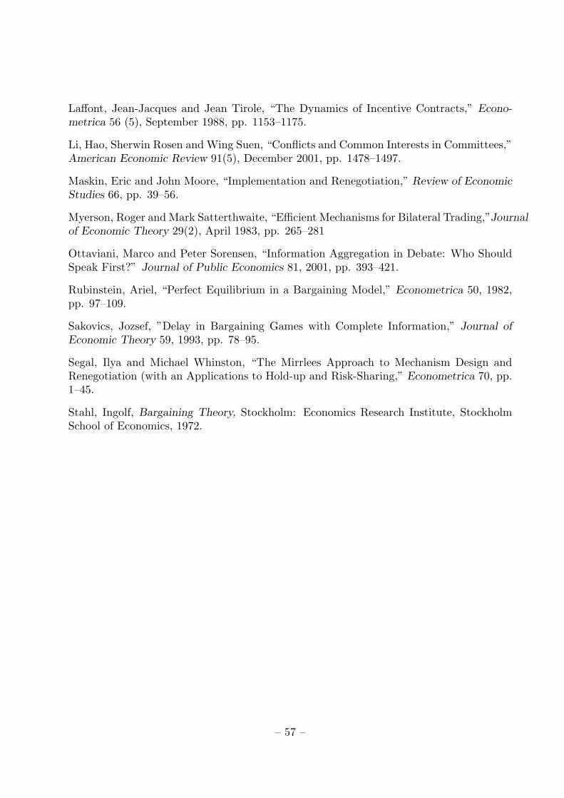
Laffont, Jean-Jacques and Jean Tirole, “The Dynamics of Incentive Contracts,” Econo-metrica 56 (5), September 1988, pp. 1153–1175.

Li, Hao, Sherwin Rosen and Wing Suen, “Conflicts and Common Interests in Committees,”American Economic Review 91(5), December 2001, pp. 1478–1497.

Maskin, Eric and John Moore, “Implementation and Renegotiation,” Review of EconomicStudies 66, pp. 39–56.

Myerson, Roger and Mark Satterthwaite, “Efficient Mechanisms for Bilateral Trading,”Journalof Economic Theory 29(2), April 1983, pp. 265–281

Ottaviani, Marco and Peter Sorensen, “Information Aggregation in Debate: Who ShouldSpeak First?” Journal of Public Economics 81, 2001, pp. 393–421.

Rubinstein, Ariel, “Perfect Equilibrium in a Bargaining Model,” Econometrica 50, 1982,pp. 97–109.

Sakovics, Jozsef, ”Delay in Bargaining Games with Complete Information,” Journal ofEconomic Theory 59, 1993, pp. 78–95.

Segal, Ilya and Michael Whinston, “The Mirrlees Approach to Mechanism Design andRenegotiation (with an Applications to Hold-up and Risk-Sharing,” Econometrica 70, pp.1–45.

Stahl, Ingolf, Bargaining Theory, Stockholm: Economics Research Institute, StockholmSchool of Economics, 1972.

– 57 –