Dehn Twist (UROP Research)

Department of Mathematics

Dehn Twist on an Annulus

Author:

Nur Nordin

Supervisor:

Prof. Sebastian van Strien

Dr. Ivan Ovsyannikov

September 25, 2014

Abstract

A Dehn twist is an example of a self-homeomorphism of a two-dimensional manifold such as an

annulus in R2. Given an annulus A and a Dehn twist f : A → A, certain algebraic properties can

be studied. In this case, the main focus will be on the quantity ‖f‖C3 ·meas(A). It is proven that

this quantity is invariant under a rigid motion and rescaling on A and also has a non-zero lower

bound for any annulus A and its Dehn twist f . The next task is to generalise these properties for

a composition of several functions that forms a Dehn twist on an annulus. In fact, the problem will

be approached by first defining a suitable value called the maximal boundary twist using the theory

of conformal maps.

1 Preliminaries

We begin by defining an annulus.

Definition 1.1 (Annulus). Let ∂iA and ∂oA be simple, closed, analytic curves in R2 such that ∂iA is

interior to ∂oA.

The region bounded by and including ∂iA and ∂oA is called annulus A.

The curves ∂iA and ∂oA are called inner and outer boundaries of A respectively.

The annulus with origin O interior to ∂iA is called centred annulus.

The annulus A ={x ∈ R2 : r ≤ |x| ≤ R

}for some r,R ∈ R, 0 < r < R is called circular annulus.

Remark 1.2. ∂iA and ∂oA are not required to be analytic. However, to avoid unnecessary complication

later, we will assume this condition for simplicity.

We define a suitable measure on an annulus A, which is simply the area of A.

Definition 1.3 (Measure). Let A be an annulus.

Then, the measure of A is defined as

meas(A) =

∫ ∫A

dx dy (1.1)

We will focus mainly on a self-homeomorphism on an annulus called a Dehn twist.

Definition 1.4 (Dehn Twist). Let A be an annulus.

f : A→ A is a Dehn twist if and only if

1. f is homeomorphism;

2. f |∂iA ≡ id∂iA and f |∂oA ≡ id∂oA;

3. for any curve L ⊂ A with endpoints on ∂iA and ∂oA, f(L) is non-homotopic to L.

The notion of a winding of a curve will be widely used in relation to a Dehn twist. For simplicity, we

will only consider the winding around origin O.

Definition 1.5 (Winding Number). Let L ⊂ R2 be a curve not passing through the origin O and

parametrised by γ : [a, b]→ R2.

Let θ : [a, b]→ R be the continuous angular coordinate of points on L.

The winding number of L about O is defined as

W (L) =θ(b)− θ(a)

2π(1.2)

L has a winding about O if and only if |W (L)| ≥ 1.

1

The following example demonstrates a Dehn twist on a circular annulus.

Example 1.6. Let A ={x ∈ R2 : 1 ≤ |x| ≤ 2

}.

Define f : A→ A in polar coordinate as

f(r, θ) = (r, θ + 2π(r − 1)) for (r, θ) ∈ [1, 2]× [0, 2π)

It is easy to check that f is a homeomorphism.

Also, note that f(1, θ) = (1, θ) and f(2, θ) = (2, θ + 2π) ≡ (2, θ) for any θ ∈ [0, 2π), so both boundaries

of A are fixed under f .

Intuitively, for any circle Cr ={x ∈ R2 : |x| = r

}in A for some r ∈ [1, 2], f rotates Cr through 2π(2−r)

anticlockwise about the origin O. Thus, for any curve L ⊂ A connecting a point on ∂iA to a point on

∂oA, f(L) takes another winding around O, so L is not homotopic to f(L).

Figure 1.1: Several curves L ⊂ A mapped under f

Remark 1.7. The fact that f(L) is not homotopic to L if and only if W (f(L)) = W (L) is geometrically

obvious. However, it will be proven later in Proposition 2.1.

We introduce a norm of a function as the following:

Definition 1.8 (C3 Norm). Let K ⊂ R2 be compact, and f : K → R2 be a C3 function.

The C3 norm of f is defined as

‖f‖C3 = supx∈K, u∈S1

∣∣∣∣ d3

dt3f(x+ tu)

∣∣∣t=0

∣∣∣∣ (1.3)

or equivalently,

‖f‖C3 = supx∈K, (u1,u2)∈S1

∣∣∣∣∣3∑i=0

(3

i

)ui1u

3−i2

∂3

∂xi∂y3−i f(x)

∣∣∣∣∣ (1.4)

Remark 1.9. Since K × S1 is compact and f is a C3 function, the supremum exists. So, ‖f‖C3 is well-

defined.

One can prove easily that it is a seminorm, but not a norm. However, it will be called norm for

convenience.

We will investigate the norm on a Dehn twist f on an annulus A. From now, we will consider f to be a

C3 function.

2 Algebraic and Geometric Properties of a Dehn Twist

We will analyse the properties of a Dehn twist on an annulus, together with its norm.

2

Proposition 2.1. Let A be a centred annulus.

Let L0, L1 ⊂ A be curves parametrized by γ0, γ1 : [a, b] → A respectively such that γ0(a) = γ1(a) ∈ ∂iAand γ0(b) = γ1(b) ∈ ∂oA.

Then, L0 is homotopic to L1 if and only if W (L0) = W (L1).

Proof. Suppose that L0 is homotopic to L1. Let θ0(s) and θ1(s) be the corresponding continuous angular

coordinate of L0 and L1 respectively. Since L0 and L1 have the same endpoints, we have θ1(a) = θ0(a)

and θ1(b) = θ0(b) + 2k1π for some k1 ∈ Z. Thus, W (L1) = W (L0) + k1. Let F : [0, 1] × [a, b] → A

be the homotopy between L0 and L1. Let Lt ⊂ A be the curve parametrized by γt : [a, b] → A

such that γt(s) = F (t, s). Let θt(s) be the corresponding continuous angular coordinate of Lt. The

continuity of θt(s) is certain since F is continuous. Consider W (Lt). Note that for all t ∈ [0, 1], we

have W (Lt) = W (L0) + kt for some kt ∈ Z by using similar argument for L1 as previous. Also, W (Lt)

is continuous for all t ∈ [0, 1], and so W (Lt) −W (L0). Since Z is discrete, W (Lt) −W (L0) must be a

constant function on [0, 1]; otherwise W (Lt) will be discontinuous. Since W (Lt)−W (L0) = 0 at t = 0,

we have W (Lt) = W (L0) for all t ∈ [0, 1], thus W (L1) = 0.

Conversely, suppose that W (L0) = W (L1). Consider a conformal homeomorphism φ : A→ A∗ where A∗

is a circular annulus {x ∈ R2 : 1 ≤ |x| ≤ R} for some R > 1. Let r0(s) and r1(s) be the radial coordinate

and Θ0(s) and Θ1(s) be the continuous angular coordinate of φ(L0) and φ(L1) respectively. It is easy

to deduce that W (φ(L0)) = W (φ(L1)). Thus, we have that Θ0(a) = Θ1(a) and Θ0(b) = Θ1(b). Define

F ∗ : [0, 1]× [x0, x1]→ A∗ as

F ∗(t, s) = ((1− t)r0(s) + tr1(s), (1− t)Θ0(s) + tΘ1(s))

in polar coordinate. Note that F ∗ is continuous since r0, r1,Θ0 and Θ1 are continuous, F ∗(0, s) = γ0(s)

and F ∗(1, s) = γ1(s), and the curves defined by F ∗(t, s) has the same endpoints for all t ∈ [0, 1]. Thus,

F ∗ is a homotopy between φ(L0) and φ(L1). Hence, F ≡ φ−1 ◦ F ∗ is a homotopy between L0 and L1.

So, L0 is homotopic to L1.

Remark 2.2. The definition of conformal map will be given formally in Definition 5.1 later.

Such conformal map φ : A→ A∗ exists based on Theorem 5.9 that will be formally stated later.

In fact, given that Lθ is the radial line of polar angle θ ∈ [0, 2π) in A∗, the set of curves φ−1(Lθ)

in A forms a set of non-intersecting curves connecting the boundaries of A with each labelled with

parameter θ ∈ [0, 2π). Thus, it is not possible for W (φ(L1)) = W (φ(L0)) + k for some non-zero integer

k, because otherwise, one of the curves L0 and L1 will have additional winding around O, contradicting

W (L0) = W (L1).

Proposition 2.3. Let A be an annulus.

Then, there exists a point p ∈ ∂iA such that the outward normal of ∂iA at x first intersects ∂oA.

Proof. Let γ : [0, 1]→ ∂iA be a parametrization of ∂iA. Consider X(t) = πx◦γ(t) which is the projection

of ∂iA onto the x-axis. Let x0 = sup[0,1]

{X(t)}. Note that because γ is continuous by definition of ∂iA,

such value is attained on ∂iA. Let p = (x0, y0) be the corresponding point on ∂iA. Note that since x0

is the maximum point, we have X ′ = 0 at p. Thus, the line x = x0 is tangential to ∂iA at p, and so

the normal line at p is parallel to x-axis. Since p corresponds to point with maximum x-coordinate, its

outward normal will never intersect ∂iA again. Because ∂iA is interior to ∂oA, the normal eventually

intersects ∂oA.

Remark 2.4. The normal line in an annulus A as in Proposition 2.3 is often considered under a Dehn

twist f because it is easy to study its image under f . For simplicity, the annulus A is transformed into

3

another annulus A∗ under rigid motion (translation and rotation) and rescaling, so that A∗ has desiring

properties such that A∗ is a centred annulus and the said normal line is mapped onto the positive x-axis.

It is worth to define such line at this point.

Definition 2.5 (Standard Spoke). Let A be a centred annulus.

Let L0 = {(x, 0) ∈ R2 : x ∈ [x0, x1]} be a line such that

1. (x0, 0) ∈ ∂iA and (x1, 0) ∈ ∂oA;

2. L0 ⊂ A;

3. L0 is normal to ∂iA at (x0, 0);

for some x0, x1 ∈ R, 0 < x0 < x1.

Then, L0 is called a standard spoke of A.

Remark 2.6. From Proposition 2.3, any annulus A can be transformed to a new annulus A∗ under a rigid

motion so that A∗ has a standard spoke L0. The choice of the standard spoke L0 is arbitrary depending

on the rigid motion. In fact, the shortest line segment in A which connects the boundaries can be made

into a standard spoke as well.

Proposition 2.7. Let A be an annulus.

Then, the shortest line segment connecting ∂iA and ∂0A lies in A and is normal to both boundaries at

the endpoints.

Proof. First, we will justify that in any annulus A, the shortest line segment connecting the boundaries

exists and lies inside A. Note that the boundaries ∂iA and ∂oA are compact sets in R2, and the Euclidean

distance d2 : ∂iA × ∂oA → R is continuous. Hence, by continuity of a function on a compact set, d2

attains its infimum on the set ∂iA × ∂oA. Let xi ∈ ∂iA and xo ∈ ∂oA be the points in which d2 is

the minimum, and let L be the line segment connecting them. Note that since ∂iA is interior to ∂oA,

we have that xi 6= xo, so L is a proper line segment. By definition of L as the shortest line segment

connecting the boundaries, L does not intersect both boundaries except at the endpoints; otherwise, the

line segment connecting the point of intersection and one of the endpoints will be shorter than L. Since

∂iA is interior to ∂oA, it is easy to see that L lies in A.

Note that since we can apply rigid motion to A without changing the distance between any two points,

without loss of generality, we can assume that L lies on the positive x-axis for simplicity. So, xi = (xi, 0)

xo = (xo, 0) for some xi, x0 ∈ R and xo > xi > 0. Let γ : [0, 1] → ∂iA the parametrization of ∂iA, and

define (x(t), y(t)) = γ(t) as the projection of ∂iA onto the corresponding axes. The tangent vector of ∂iA

is given by (x′(t), y′(t)). Suppose that at xi, L is not normal to ∂iA, and thus x′ 6= 0 at xi. By continuity

of γ(t), in a small neighbourhood of xi, there exists a point x = (x, y) ∈ ∂iA such that x > xi. By using

triangle inequality, it is clear that the distance between xo and x is less than the distance between xo

and xi. This is a contradiction on L being the shortest. Similarly, we can show that L is normal to ∂oA

at xo using the same argument.

The image of a standard spoke L0 under a Dehn twist f has useful properties.

Proposition 2.8. Let A be a centred annulus, L0 = {(x, 0) ∈ R2 : x ∈ [x0, x1]} be a standard spoke of

A and f : A→ A be a Dehn twist.

Then, f(L0) has a winding around the origin O.

Proof. By definition of a Dehn twist, f(L0) is not homotopic to L0. From Proposition 2.1, we have

W (f(L0)) 6= W (L0) = 0, and thus W (f(L0)) = k for some k ∈ Z \ {0}. By definition, f(L0) has a

winding around the origin O.

4


A and f : A→ A be a Dehn twist which is C1 diffeomorphism.

Then, the tangent vector of f(L0) at (x0, 0) is not tangential to ∂iA at (x0, 0).

Proof. Since f is a C1 diffeomorphism, the Jacobian matrix Dfx is non-singular for any x ∈ A. Let

γ : [0, 1]→ A be a parametrization of a curve L in A and f ◦ γ(t) be the parametrization of f(L). It is

easy to check that the tangent vector of f(L) is

(f ◦ γ)′(t) = Dfγ(t) · γ′(t)

So, the tangent vector of any curve L is mapped by Dfx to the tangent vector of its image f(L).

Consider point (x0, 0). Then, Df(x0,0) : R2 → R2 is a bijection since the matrix Df(x0,0) is invertible.

Thus, Df(x0,0) maps two linearly independent vectors in R2 to two linearly independent vectors in R2.

Consider ∂iA. Note that by definition of L0, the tangent vector of ∂iA at (x0, 0) is perpendicular to the

x-axis. Since f |∂iA ≡ id∂iA, we have that the tangent vector of ∂iA at (x0, 0) is mapped by Df(x0,0) onto

another vector perpendicular to x-axis as well.

Now, let (X(x), Y (x)) = f(x, 0) for x ∈ [x0, x1] which parametrizes f(L0). Note that the tangent vector

of f(L0) is (X ′, Y ′) = Df(x,0) · e1. Consider again (x0, 0). Suppose that the tangent vector of f(L0)

at (x0, 0) is tangential to ∂iA, or equivalently, perpendicular to the x-axis. So, Df(x0,0) maps e1 to a

vector perpendicular to the x-axis. Thus, Df(x0,0) maps two linearly independent vectors to two linearly

dependent vectors. This contradicts Df(x0,0) being bijective.

Hence, the tangent vector of f(L0) at (x0, 0) is not tangential to ∂iA at (x0, 0).

Proposition 2.9 requires f to be C1 diffeomorphism. Starting now, we will assume a Dehn twist f to be

a C1 diffeomorphism for simplicity.



Define X(x) = πx ◦ f(x, 0) and Y (x) = πy ◦ f(x, 0) for x ∈ [x0, x1] as the projection of f(L0) onto x-axis

and y-axis respectively.

Then, X and Y each has two turning points of positive and negative values on (x0, x1).

Proof. By definition of a Dehn twist, L0 is not homotopic to f(L0). Thus, f(L0) must have a winding

around the origin O from Proposition 2.8. It is clear that f(L0) must intersect the negative x-axis,

positive y-axis and negative y-axis each at least once to complete the winding.

Figure 2.1: Standard spoke L0 and its image f(L0) on centred annulus A

5

Consider X(x). Since f is a Dehn twist, X(x0) = x0 and X(x1) = x1. Note that by Proposition 2.9, the

tangent vector of f(L0) at (x0, 0) is not tangential to ∂iA, thus X ′(x0) 6= 0. Also, note that X ′(x0) > 0;

otherwise, in a small neigbourhood of x0, (X,Y ) will be interior to ∂iA which is not possible since

f(L0) ⊂ A. Thus, for sufficiently small ε > 0, we have X(x0 + ε) > x0. Let p ∈ (x0, x1) be the point

such that f(L0) intersects the negative x-axis, so we have X(p) < 0. By Intermediate Value Theorem,

since X is continuous on [x0 + ε, p], there exists a point k ∈ (x0 + ε, p) such that X(k) = x0. Without

loss of generality, we can choose k to be point that X > x0 on (x0, k). By Rolle’s Theorem, there exists

a point a ∈ (x0, k) such that X ′(a) = 0. Since a ∈ (x0, k), by construction, we have X(a) > 0.

Let q, r ∈ (x0, x1) be the points such that f(L0) intersects the positive and negative y-axis respectively.

Without loss of generality, again, we can choose points q and r such that X < 0 on (q, r). So, we have

X(q) = X(r) = 0. By Rolle’s Theorem, there exists b ∈ (q, r) such that X ′(b) = 0. Since b ∈ (q, r), by

construction, we have X(b) < 0.

We can use similar argument on Y (x) by using Rolle’s Theorem on the part of the curve f(L0) where

s, t ∈ [x0, x1] are the points such that f(L0) intersects the positive and negative x-axis respectively and

Y > 0 on (s, t), and also on another part where u, v ∈ [x0, x1] are the points such that f(L0) intersects

the negative and positive x-axis respectively and Y < 0 on (u, v).



Define X(x) = πx ◦ f(x, 0) and Y (x) = πy ◦ f(x, 0) for x ∈ [x0, x1] as the projection of f(L0) onto x-axis

and y-axis respectively.

Then,

‖f‖C3 ≥ sup[x0,x1]

|X ′′′|

‖f‖C3 ≥ sup[x0,x1]

|Y ′′′|

Proof. Recall the definition of C3 norm as

‖f‖C3 = supx∈K, (u1,u2)∈S1

∣∣∣∣∣3∑i=0

(3

i

)ui1u

3−i2

∂3

∂xi∂y3−i f(x)

∣∣∣∣∣Choosing u = e1 leads to

‖f‖C3 ≥ supx∈[x0,x1]

∣∣∣∣ ∂3

∂x3f(x, 0)

∣∣∣∣Note that

(X ′′′(x), Y ′′′(x)) =∂3

∂x3f(x, 0)

=⇒ |(X ′′′, Y ′′′)| =∣∣∣∣ ∂3

∂x3f(x, 0)

∣∣∣∣=⇒ |X ′′′| ≤

∣∣∣∣ ∂3

∂x3f(x, 0)

∣∣∣∣ and |Y ′′′| ≤∣∣∣∣ ∂3

∂x3f(x, 0)

∣∣∣∣for all x ∈ [x0, x1].

Taking the supremum over [x0, x1] and by previous inequality, we obtain the result.

As stated previously, for a given annulus A, it is possible to apply rigid motion and rescaling on A to

obtain a new annulus A∗. The next propositions relate the Dehn twists on A and A∗, and also their

norm.

6

Proposition 2.12. Let A be an annulus and f : A→ A be a Dehn twist.

Let T : A→ A∗ be a homeomorphism where A∗ is an annulus such that T (∂iA) = ∂iA∗ and

T (∂oA) = ∂oA∗.

Define f∗ : A∗ → A∗ as f∗ ≡ T ◦ f ◦ T−1.

Then, f∗ is a Dehn twist on A∗ such that

Proof. It is easy to check that f∗ is a homeomorphism and f∗ fixes all points on the boundaries of A∗

by definition of a Dehn twist f and the properties of T .

Suppose that there exists a curve L∗ ∈ A∗ with endpoints x∗0 ∈ ∂iA∗ and x∗1 ∈ ∂oA∗ such that f∗(L∗) is

homotopic to L∗. Let γ∗ : [0, 1] → A∗ be the parametrization of L∗. Let F : [0, 1] × [0, 1] → A∗ be the

homotopy, so F (s, 0) = γ∗(s), F (s, 1) = f∗ ◦γ∗(s), F (0, t) = x∗0 and F (1, t) = x∗1. Consider L = T−1(L∗)

parametrized by γ ≡ T−1 ◦ γ∗ and so its image f(L) is parametrised by f ◦ γ ≡ T−1 ◦ f∗ ◦ γ. Also, L has

each endpoint at each boundary since ∂iA = T−1(∂iA∗) and ∂oA = T−1(∂oA

∗). It is easy to check that

T−1 ◦ F is a homotopy between γ and f ◦ γ. However, this contradicts the definition of a Dehn twist f

that L is not homotopic to f(L).

Hence, f∗ is a Dehn twist.


Let T : A→ A∗ be a homeomorphism where A∗ is an annulus such that T (∂iA) = ∂iA∗ and

T (∂oA) = ∂oA∗.

Let f∗ : A∗ → A∗ be the corresponding Dehn twist on A∗ where f∗ ≡ T ◦ f ◦ T−1.

(a) If T (x) = x+ τ for some τ ∈ R2, then

‖f∗‖C3 = ‖f‖C3

(b) If T (x) = Rx for some rotation matrix R, then

‖f∗‖C3 = ‖f‖C3

(c) If T (x) = λx for some λ ∈ R+, then

‖f∗‖C3 =1

λ2‖f‖C3

Proof. (a) Consider x∗ ∈ A∗ and u ∈ S1. Note that

f∗(x∗ + tu) = a+ f(x∗ − a+ tu)

=⇒ d3

dt3f∗(x∗ + tu) =

d3

dt3f(x∗ − a+ tu)

Since A∗ = T (A) and T is bijective, we have

‖f∗‖C3 = supx∗∈A∗, u∈S1

∣∣∣∣ d3

dt3f∗(x∗ + tu)

∣∣∣t=0

∣∣∣∣= supx∗∈A∗, u∈S1

∣∣∣∣ d3

dt3f(x∗ − a+ tu)

∣∣∣t=0

∣∣∣∣= supx∈A, u∈S1

∣∣∣∣ d3

dt3f(x+ tu)

∣∣∣t=0

∣∣∣∣= ‖f‖C3

7

(b) Consider x∗ ∈ A∗ and u ∈ S1. Note that

f∗(x∗ + tu) = Rf(R−1x∗ + tR−1u)

=⇒ d3

dt3f∗(x∗ + tu) = R

d3

dt3f(R−1x∗ + tR−1u)

=⇒∣∣∣∣ d3

dt3f∗(x∗ + tu)

∣∣∣∣ =

∣∣∣∣ d3


∣∣∣∣since R preserves the length. Note that R−1u ∈ S1. Since A∗ = T (A) and T is bijective, we have

‖f∗‖C3 = supx∗∈A∗, u∈S1

∣∣∣∣ d3

dt3f∗(x∗ + tu)

∣∣∣t=0

∣∣∣∣= supx∗∈A∗, u∈S1

∣∣∣∣ d3


∣∣∣∣= supx∈A, v∈S1

∣∣∣∣ d3

dt3f(x+ tv)

∣∣∣t=0

∣∣∣∣= ‖f‖C3

(c) Consider x∗ ∈ A∗ and u ∈ S1. Note that

f∗(x∗ + tu) = λf

(1

λx∗ +

t

λu

)Thus, we have

d3

dt3f∗(x∗ + tu)

∣∣∣t=0

= λd3

dt3f

(1

λx∗ +

t

λu

) ∣∣∣∣t=0

= λ

3∑i=0

(3

i

)(u1

λ

)i (u2

λ

)3−i ∂3

∂xi∂y3−i f

(1

λx∗)

=1

λ2

3∑i=0

(3

i

)ui1u

3−i2

∂3

∂xi∂y3−i f

(1

λx∗)

=1

λ2

d3

dt3f

(1

λx∗ + tu

) ∣∣∣∣t=0

Since A∗ = T (A) and T is bijective, we have

‖f∗‖C3 = supx∗∈A∗, u∈S1

∣∣∣∣ d3

dt3f∗(x∗ + tu)

∣∣∣t=0

∣∣∣∣= supx∗∈A∗, u∈S1

∣∣∣∣ 1

λ2

d3

dt3f

(1

λx∗ + tu

) ∣∣∣∣t=0

∣∣∣∣=

1

λ2sup

x∈A, u∈S1

∣∣∣∣ d3

dt3f(x+ tu)

∣∣∣t=0

∣∣∣∣=

1

λ2‖f‖C3

Remark 2.14. Propositions 2.3 and 2.13 show that we can always transform any annulus A under a rigid

motion into a new annulus A∗, so that A∗ is a centred annulus and has a standard spoke L0, without

changing the value of the norm. Hence, it is sufficient to consider annulus A which is centred and has a

standard spoke L0 when working with the norm of any Dehn twist f on A.

8

Corollary 2.15. Let A be an annulus and f : A→ A be a Dehn twist.

Let A∗ be the image of A under a sequence of rigid motions (translation and rotation) and rescalings,

and f∗ : A∗ → A∗ be the corresponding Dehn twist.

Then,

‖f‖C3 ·meas(A) = ‖f∗‖C3 ·meas(A∗)

Proof. From Proposition 2.13, any rigid motion on any annulus A does not change the value of the norm

of the Dehn twist f . Thus, the value of the norm changes due to the overall rescaling of A. Let λ be the

resulting scale factor of all rescalings of A. So,

‖f∗‖C3 =1

λ2‖f‖C3

Similarly, meas(A), which is the area of A is not affected by any rigid motion, but it does change due

to the overall rescaling of A. It is easy to check that

meas(A∗) = λ2 meas(A)

Multiplying them together and we obtain the result.

3 Quantity ‖f‖C3 ·meas(A)

Corollary 2.15 states that for any annulus A and a Dehn twist f , the value of ‖f‖C3 ·meas(A) remains

constant regardless of rigid motions and rescalings on A. In fact, we are interested in the value of

‖f‖C3 ·meas(A) for any annulus A and its Dehn twist f .

First, given an annulus A, we need to consider the suitable lower bound for ‖f‖C3 for any Dehn twist f

on A.



Then,

‖f‖C3 6= 0

Proof. Suppose the contrary that ‖f‖C3 = 0. Thus, for all x ∈ A and u = (u1, u2) ∈ S1, we have

3∑i=0

(3

i

)ui1u

3−i2

∂3

∂xi∂y3−i f(x) = 0

In fact, for any v = (v1, v2) ∈ R2, by considering its unit vector, we deduce that

3∑i=0

(3

i

)vi1v

3−i2

∂3

∂xi∂y3−i f(x) = 0

Consider any point x0 = (x0, y0) ∈ A. By using Taylor’s Theorem on f about x0, we have

f(x) =

3∑k=0

k∑i=0

(k

i

)(x− x0)i(y − y0)k−i

∂k

∂xi∂yk−if(x0) +R3

where

R3 =1

2

∫ 1

0

(1− t)23∑i=0

(3

i

)(x− x0)i(y − y0)3−i ∂3

∂xi∂y3−i f (x0 + t(x− x0)) dt

9

From previous, the integrand is 0, so we have that R3 = 0 for all x ∈ A. Thus, we have that f is a

polynomial of degree at most 2 in R2.

Let X(x) = πx ◦ f(x, 0) for x ∈ [x0, x1] which is the projection of f(L0) onto the x-axis. Since f has

degree at most 2, X is a polynomial of x of degree at most 2. By Proposition 2.10, X has at least two

turning points on [x0, x1]. This contradicts X having degree at most 2 which has at most one turning

point.

Proposition 3.1 only tells that for any Dehn twist f on an annulus A, it holds that ‖f‖C3 > 0. However,

we need a non-trivial lower bound for f in this case.



Then,

‖f‖C3 >1

(x1 − x0)2

Proof. Consider X(x) = πx ◦ f(x, 0) for x ∈ [x0, x1] which is the projection of f(L0) onto the x-axis.

Note that by definition of a Dehn twist, f fixes all points on both boundaries, so X(x0) = x0 and

X(x1) = x1. By Proposition 2.10, X has two turning points of positive and negative values on (x0, x1).

Let p, q ∈ (x0, x1) be the turning points of positive and negative values respectively. Without loss of

generality, let p < q.

By Rolle’s Theorem, since X ′(p) = X ′(q) = 0, there exists a ∈ (p, q) such that X ′′(a) = 0.

Now, we claim that there exists b ∈ (q, x1) such that |X ′(b)| ≥ 1. Otherwise, suppose the contrary that

on (q, x1), we have |X ′(x)| < 1. Then

X(x1)−X(q) =

∫ x1

q

X ′(x) dx

=⇒ |x1 −X(q)| ≤∫ x1

q

|X ′(x)| dx <∫ x1

q

dx = x1 − q < x1

But, since X(q) < 0, we have |x1 −X(q)| > x1, which is a contradiction.

Now, by using Mean Value Theorem, there exists c ∈ (q, b) such that

X ′′(c) =X ′(b)−X ′(q)

b− q

=X ′(b)

b− q

Again, by using Mean Value Theorem, there exists d between a and c such that

X ′′′(d) =X ′′(c)−X ′′(a)

c− a

=X ′′(c)

c− a

=X ′(b)

(b− q)(c− a)

Thus, since |b− q| < |x1 − x0| and |c− a| < |x1 − x0|, and previously |X ′(b)| ≥ 1, we have

|X ′′′(d)| > 1

(x1 − x0)2

10

By Proposition 2.11, we have

‖f‖C3 ≥ sup[x0,x1]

|X ′′′|

≥ |X ′′′(d)|

>1

(x1 − x0)2

Note that from Proposition 3.2, if ∂oA tends to be further away from ∂iA, then the lower bound for ‖f‖C3

tends to 0, which is not useful. However, meas(A) may become sufficiently big in this case. Similarly,

if ∂oA tends to be closer to ∂iA, then ‖f‖C3 tends to infinity, which is desirable. However, in this case,

meas(A) tends to 0 instead. Both cases shows that in some way, meas(A) plays the important role on

maintaining the lower bound for ‖f‖C3 ·meas(A) to remain at certain value.

Theorem 3.3. For any circular annulus A and its Dehn twist f : A→ A,

‖f‖C3 ·meas(A) > π

Proof. Let A ={x ∈ R2 : r ≤ |x| ≤ R

}for some r,R ∈ R, 0 < r < R and f : A → A be a Dehn twist.

Note that A has a standard spoke L0 ={

(x, 0) ∈ R2 : x ∈ [r,R]}

.

By Proposition 3.2, we have

‖f‖C3 >1

(R− r)2

Thus, using meas(A) = π(R2 − r2) and R+ r > R− r, we have

‖f‖C3 ·meas(A) >π(R2 − r2)

(R− r)2

= π

(R+ r

R− r

)> π

This holds for any circular annulus A and any Dehn twist f . Hence, we are done.

Theorem 3.3 can be generalised to any annulus A, but the proof is more involved, since the calculation

for meas(A) is more complicated.

Theorem 3.4. For any annulus A and its Dehn twist f : A→ A,

‖f‖C3 ·meas(A) > π

Proof. By Propositions 2.7 and 2.13, we can apply rigid motion on A so that A is a centred annulus and

the shortest line segment connecting both boundaries is a standard spoke L0 without changing the value

of ‖f‖C3 . Without loss of generality, let L0 ={

(x, 0) ∈ R2 : x ∈ [x0, x1]}

be the standard spoke of A

such that it is the shortest line segment connecting ∂iA and ∂oA. By Proposition 3.2, we have

‖f‖C3 >1

(x1 − x0)2

Now, we have to find a suitable lower bound for meas(A). Consider constructing all radial lines tangential

to ∂iA and ∂oA. The set of such radial lines will be countable. Thus, the radial lines partition A into a

countable set P of smaller regions. Now, we will choose S ⊆ P such that

11

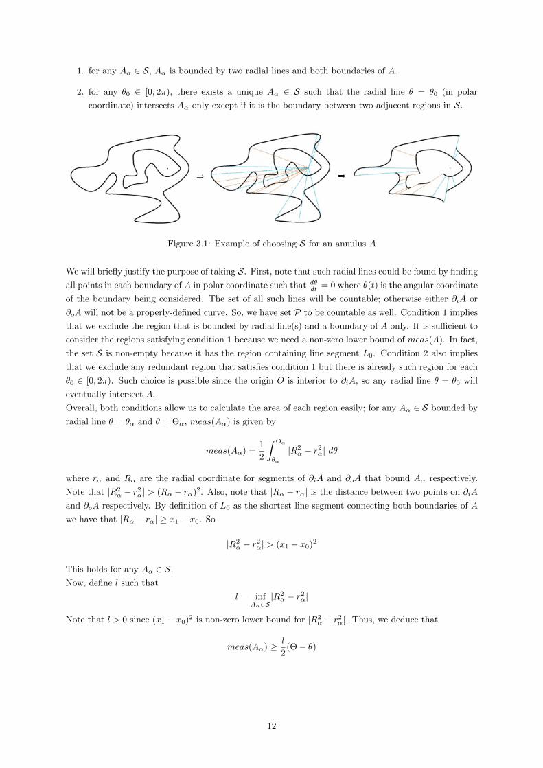
1. for any Aα ∈ S, Aα is bounded by two radial lines and both boundaries of A.

2. for any θ0 ∈ [0, 2π), there exists a unique Aα ∈ S such that the radial line θ = θ0 (in polar

coordinate) intersects Aα only except if it is the boundary between two adjacent regions in S.

Figure 3.1: Example of choosing S for an annulus A

We will briefly justify the purpose of taking S. First, note that such radial lines could be found by finding

all points in each boundary of A in polar coordinate such that dθdt = 0 where θ(t) is the angular coordinate

of the boundary being considered. The set of all such lines will be countable; otherwise either ∂iA or

∂oA will not be a properly-defined curve. So, we have set P to be countable as well. Condition 1 implies

that we exclude the region that is bounded by radial line(s) and a boundary of A only. It is sufficient to

consider the regions satisfying condition 1 because we need a non-zero lower bound of meas(A). In fact,

the set S is non-empty because it has the region containing line segment L0. Condition 2 also implies

that we exclude any redundant region that satisfies condition 1 but there is already such region for each

θ0 ∈ [0, 2π). Such choice is possible since the origin O is interior to ∂iA, so any radial line θ = θ0 will

eventually intersect A.

Overall, both conditions allow us to calculate the area of each region easily; for any Aα ∈ S bounded by

radial line θ = θα and θ = Θα, meas(Aα) is given by

meas(Aα) =1

2

∫ Θα

θα

|R2α − r2

α| dθ

where rα and Rα are the radial coordinate for segments of ∂iA and ∂oA that bound Aα respectively.

Note that |R2α − r2

α| > (Rα − rα)2. Also, note that |Rα − rα| is the distance between two points on ∂iA

and ∂oA respectively. By definition of L0 as the shortest line segment connecting both boundaries of A

we have that |Rα − rα| ≥ x1 − x0. So

|R2α − r2

α| > (x1 − x0)2

This holds for any Aα ∈ S.

Now, define l such that

l = infAα∈S

|R2α − r2

α|

Note that l > 0 since (x1 − x0)2 is non-zero lower bound for |R2α − r2

α|. Thus, we deduce that

meas(Aα) ≥ l

2(Θ− θ)

12

Now, we have that

meas(A) ≥∑Aα∈S

meas(Aα)

≥ l

2

∑Aα∈S

(Θ− θ)

= πl

since condition 2 previously implies∑Aα∈S(Θ− θ) = 2π.

Thus, we deduce that

meas(A) ≥ πl

Using the fact that l ≥ (x1 − x0)2 by definition of l as infimum, we obtain

‖f‖C3 ·meas(A) >1

(x1 − x0)2· πl

≥ π

as desired.

As a conclusion, we obtain:

Theorem 3.5. Let

C0 = inf(A,f)

(‖f‖C3 ·meas(A))

where A is an annulus and f : A→ A is its Dehn twist.

Then,

C0 > 0

Proof. This follows immediately from Theorem 3.4 which shows that C0 ≥ π.

We can possibly find the generalisation of Theorem 3.5 as following:

Conjecture 3.6. Let {Ai}ni=1 be the set of annuli and fi : Ai → Ai+1 is a C3 homeomorphism for

i = 1, 2, ..., n and An+1 = A1.

Suppose that f : A1 → A1 where f = fn ◦ fn−1 ◦ ... ◦ f1 is a Dehn twist.

Define

C0 = inf({Ai}ni=1,{fi}ni=1)

(max

i=1,2,...,n‖fi‖C3 ·

n∑i=1

meas(Ai)

)

for all such pairs of sets {Ai}ni=1 and {fi}ni=1.

Then,

C0 > 0

We will now try to prove Conjecture 3.6 if possible.

4 Form of a Dehn Twist

First of all, for Conjecture 3.6 to hold true, note that for all such pairs {Ai}ni=1 and {fi}ni=1, we have

‖fi‖C3 6= 0 for all i = 1, 2, ..., n. In other words, based on proof for Proposition 3.1, fi cannot be a linear

or quadratic polynomial in R2 for all i = 1, 2, ..., n. So, we need to prove that any composition of linear

13

and/or quadratic polynomials in R2 cannot be a Dehn twist on any annulus.

Example 1.6 shows a Dehn twist f on a circular annulus A, in which in Cartesian coordinate, f will be a

complicated function involving trigonometric functions. This shows that a Dehn twist on an annulus may

be difficult to be expressed algebraically, even by common functions, especially if the annulus is more

deviated from the circular one. Now, we may try to investigate a Dehn twist on some annulus which is

expressible by a polynomial in R2. We can prove that it is not possible for lower-degree polynomials.

For example, Proposition 3.1 shows that any Dehn twist cannot be a linear or quadratic polynomial in R2.

The following theorem is useful to prove the assertion later:

Theorem 4.1 (Bezout). Let C1 and C2 be plane algebraic curves defined by f1(x, y) = 0 and f2(x, y) = 0

respectively, where f1 and f2 are polynomials of degreee d1 and d2 respectively.

If f1 and f2 are coprime, then the number of intersections between C1 and C2 is less than or equal to

d1d2.

Theorem 4.1 is well-known in the study of plane algebraic curves and the proof can be found in pages

59-63, Robert J. Walker: Plane Algebraic Curves.

Theorem 4.2. Let A be an annulus and f : A→ A be a Dehn twist.

Then, f cannot be a polynomial of degree less than or equal to 4.

Proof. Suppose the contrary, that f is a polynomial of degree d, where d ≤ 4.

Note that we can apply rigid motion on A and the corresponding function will be a polynomial of degree

d. Without loss of generality, let A be a centred annulus and L0 = {(x, 0) ∈ R2 : x ∈ [x0, x1]} be a

standard spoke.

Consider extending f on R2. This is possible since f is a polynomial. Let f(x, y) = (f1(x, y), f2(x, y)),

where f1 or f2 are polynomials of degree d1 and d2 respectively, and d1, d2 ≤ d ≤ 4.

Consider the boundaries of A. Note that for any (x, y) ∈ ∂iA∪∂oA, we have f(x, y) = (x, y) by definition

of a Dehn twist. Let V1 = {(x, y) ∈ R2 : f1(x, y) = x} and V2 = {(x, y) ∈ R2 : f2(x, y) = y}. Thus,

∂iA ∪ ∂oA ⊆ V1 ∩ V2

or to put it simply, ∂iA and ∂oA are some parts of the intersection between algebraic curves defined by

f1(x, y) − x = 0 and f2(x, y) − y = 0. Note that ∂iA and ∂oA are infinite sets, hence by contrapositive

part of Theorem 4.1, polynomials f1(x, y)−x and f1(x, y)−y have a non-constant common factor Q(x, y)

of degree at most 4. Thus,

f1(x, y)− x ≡ Q(x, y) · h1(x, y) f2(x, y)− y ≡ Q(x, y) · h2(x, y)

for some coprime polynomials h1 and h2. Since h1 and h2 are coprime, then again by Theorem 4.1, the

set of intersection between algebraic curves defined by h1(x, y) = 0 and h2(x, y) = 0 is finite. Let C be

the algebraic curve defined by Q(x, y) = 0. Therefore, we deduce that

V1 ∩ V2 = C ∪ {(x, y) ∈ R2 : h1(x, y) = h2(x, y) = 0}

Since each ∂iA and ∂oA is connected and infinite set, then

∂iA ∪ ∂oA ⊆ C

14

or in other words, the boundaries are a part of the curve C. Note that we can find a line passing through

the origin O which is not a part of C and intersects each boundary of A at two distinct points; otherwise,

the degree of Q will be infinite. Hence, since ∂iA ∪ ∂oA ⊆ C, the line intersects C at least at 4 points.

By Theorem 4.1, Q cannot have degree less than 4; otherwise, there cannot be more than 3 points of

intersection. Hence, Q must have degree 4. Consequently, h1 and h2 must be a non-zero constant. So,

we have that

f(x, y) = (h1Q(x, y) + x, h2Q(x, y) + y)

for some h1, h2 ∈ R \ {0}.Consider f(L0). Define X(x) = f1(x, 0) and Y (x) = f2(x, 0) for x ∈ [x0, x1] as the projection of f(L0)

onto x-axis and y-axis respectively. We have

X(x) = h1Q(x, 0) + x Y (x) = h2Q(x, 0)

=⇒ X =h1

h2Y + x

=⇒ X > kY

where k = h1

h2and since x > 0. This means that for all points on f(L0) where X = 0, the corresponding

Y will have the same sign. But, since f(L0) must have a winding around the origin O, f(L0) must

intersect the positive and negative y-axis each at least once. This is a contradiction.

Hence, f cannot be a polynomial of degree less than or equal to 4.

Remark 4.3. Theorem 4.2 proves that a composition of two linear and/or quadratic functions in R2

cannot be a Dehn twist on any annulus. However, it is not possible to prove the same assertion for

a composition of more than two such functions in similar way. One reason, for example, the coprime

polynomials h1 and h2 as defined in the proof above may not be constant, and so we cannot determine

the sign of k to use the argument for contradiction.

It is worth to mention that it is still a question whether there exists a polynomial in R2 which is a Dehn

twist on some annulus. For now, we will leave it and try to look for a suitable tool to prove Conjecture

3.6.

5 Twist of a Function on Annulus

In this section, we will investigate the definition of a twist of a function on an annulus. Before that,

we have to be familiar with conformal maps and extremal length of a set of curves in R2. Now, we will

interchange between R2 and C for convenience.

Definition 5.1 (Conformal Map). Let D ⊆ C and φ : D → C be a C1 function.

φ is conformal at z0 ∈ D if and only if there exist r ∈ R+ and θ ∈ [0, 2π) such that for all C1 curves

γ : I → D for some open interval I ⊂ R and γ(t0) = z0 for some t0 ∈ I,

|(φ ◦ γ)′(t0)| = r · |γ′(t0)| (5.1)

arg ((φ ◦ γ)′(t0)) = θ + arg(γ′(t0)) (5.2)

φ is conformal on D if and only if φ is conformal at any point z ∈ D.

The following proposition about conformal maps is well-known:

Proposition 5.2. Let D ⊆ C and φ : D → C be a C1 function.

φ is conformal at z0 ∈ D if and only if φ is holomorphic and has non-zero derivative at z0 ∈ D.

15

Proof. As usual notation, let z = x+ iy and φ(z) = u(x, y) + iv(x, y) where x, y ∈ R.

Suppose that φ is conformal at z0 ∈ D as in Definition 5.1. Consider γ1 : (−δ1, δ1) → D defined by

γ1(t) = z0 + t for some δ1 > 0. It is easy to check that that γ1(0) = z0 and (φ ◦ γ1)′(0) = φx(z0). Also,

consider γ2 : (−δ2, δ2) → D defined by γ2(t) = z0 + it for some δ2 > 0. We have that γ2(0) = z0 and

(φ◦γ2)′(0) = φy(z0). Note that |γ′1(0)| = |γ′2(0)| = 1 and arg(γ′1(0)) = π2 + arg(γ′1(0)), so we deduce that

γ′1(0) = −iγ′2(0)

By conformality of φ, using equation (5.1), we have

arg(γ′1(0)) =π

2+ arg(γ′1(0))

=⇒ arg((φ ◦ γ1)′(0))− θ =π

2+ arg((φ ◦ γ2)′(0))− θ

=⇒ arg(φx(z0)) =π

2+ arg(φy(z0))

and thus, φx(z0) = −kiφy(z0) for some k > 0. By conformality of φ, using equation (5.2), we have

φx(z0) = −kiφy(z0)

=⇒ |(φ ◦ γ1)′(0)| = k|(φ ◦ γ2)′(0)|

=⇒ r · |γ′1(0)| = kr · |γ′2(0)|

=⇒ k = 1

since |γ′1(0)| = |γ′2(0)| = 1 and r > 0. So, we have

φx(z0) = −iφy(z0)

=⇒ φz = 0

Hence, φ satisfies Cauchy-Riemann conditions at z0. Since u(x, y) and v(x, y) are continuously differen-

tiable on D, we deduce that φ is holomorphic at z0.

By chain rule and equation (5.2),

(φ ◦ γ1)′(0) = φ′(γ1(0)) · γ′1(0)

=⇒ |(φ ◦ γ1)′(0)| = |φz(z0)| · |γ′1(0)|

=⇒ r · |γ′1(0)| = |φz(z0)| · |γ′1(0)|

=⇒ |φz(z0)| = r > 0

Hence, φz(z0) 6= 0.

Conversely, suppose that φ is holomorphic at z0 and φz(z0) 6= 0. Consider γ : I → D passing through z0

at t0 ∈ I for some open interval I ⊂ R. By chain rule,

(φ ◦ γ)′(t0) = φz(z0) · γ′(t0)

Set r = |φz(z0)| > 0 and θ = arg(φz(z0)) ∈ [0, 2π). Using the chain rule, it is easy to see that

|(φ ◦ γ)′(t0)| = r · |γ′(t0)| arg((φ ◦ γ)′(t0)) = θ + arg(γ′(t0))

Hence, φ is conformal at z0.

16

Definition 5.3 (Extremal Length). Let D ⊆ C and Γ is a set of curves in D.

Consider ρ : D → R such that

1. ρ is Borel-measurable;

2. ρ(z) ≥ 0 for any z ∈ D;

3.∫Dρ2 dx dy is finite and non-zero.

Such ρ is said to be allowable.

Define Lγ(ρ) =∫γρ |dz| for any γ ∈ Γ.

Define

L(ρ) = infγ∈Γ

Lγ(ρ) (5.3)

A(p) =

∫D

ρ2 dx dy (5.4)

Then, the extremal length, λ(Γ) is defined as

λ(Γ) = supρ

(L(ρ))2

A(ρ)(5.5)

Example 5.4. Let A = {z ∈ C : R1 ≤ |z| ≤ R2}, where R2 > R1 > 0.

Let Γ be the set of curves in A whose the endpoints are on the inner and outer boundaries respectively.

Consider any allowable ρ as defined in Definition 5.3 and let γ0 = {z ∈ C : z = x, x ∈ [R1, R2]} ∈ Γ.

Then, using polar coordinates,

Lγ0(ρ) =

∫ R2

R1

ρ dr

=⇒ L(ρ) ≤∫ R2

R1

ρ dr

=⇒ 2πL(ρ) ≤∫ 2π

0

∫ R2

R1

ρ dr dθ

=⇒ 4π2(L(ρ))2 ≤

(∫ 2π

0

∫ R2

R1

ρ dr dθ

)2

By using Cauchy-Schwarz inequality,(∫ 2π

0

∫ R2

R1

ρ dr dθ

)2

≤

(∫ 2π

0

∫ R2

R1

ρ2 r dr dθ

)·

(∫ 2π

0

∫ R2

R1

1

rdr dθ

)

= A(ρ) · 2π log

(R2

R1

)with equality if and only if ρ = k

r for any k ∈ R+.

Hence, using the inequalities and taking the supremum over all ρ, we have

(L(ρ))2

A(ρ)≤ 1

2πlog

(R2

R1

)=⇒ λ(Γ) ≤ 1

2πlog

(R2

R1

)Now, take ρ0 = 1

r in polar coordinate and consider any γ ∈ Γ. Using |dz|2 = dr2 + r2dθ2 =⇒ |dz| ≥ dr,

17

we have

Lγ(ρ0) =

∫γ

ρ0 |dz|

≥∫ R2

R1

ρ0 dr

= log

(R2

R1

)Thus, taking the infimum over all γ ∈ Γ, we have

L(ρ0) ≥ log

(R2

R1

)Also, it is easy to check that

A(ρ0) = 2π log

(R2

R1

)Hence, by definition of supremum, we have

λ(Γ) ≥ (L(ρ0))2

A(ρ0)

≥ 1

2πlog

(R2

R1

)By both, we conclude that

λ(Γ) =1

2πlog

(R2

R1

)Also, note that using the same ρ0 and γ0, it is easy to calculate that

(Lγ0(ρ0))2

A(ρ0)=

1

2πlog

(R2

R1

)Hence, λ(Γ) attains its value by those ρ0 and γ0.

In Example 5.4, the extremal length is attained by some function and curve. In fact, there are other

pairs of function and curve such that this is true, such that ρ = kr for any k ∈ R+ and γ as any radial

line segment connecting both boundaries in A. These pairs of function and curve are worth to be defined

properly.

Definition 5.5 (Extremal Pair). Let D ⊆ C, Γ be a set of curves in D, and λ(Γ) be its extremal length.

Suppose that there exist a function ρ0 and curve γ0 ∈ Γ such that

λ(Γ) =((Lγ0(ρ0))

2

A(ρ0)

Then, (ρ0, γ0) is called an extremal pair.

ρ0 is an extremal function with corresponding extremal curve γ0.

Extremal length is invariant under conformal maps based on following:

Theorem 5.6. Let D,D∗ ⊆ C and φ : D → D∗ be a bijective conformal map.

Let Γ be a set of curves in D and φ(Γ) be the set of images of the curves in D∗.

Then,

λ(φ(Γ)) = λ(Γ)

18

Proof. For convenience, we denote z = x+ yi ∈ D and w = u+ vi ∈ D∗.Consider any allowable function ρ : D → R. Define the corresponding function ρ∗ : D∗ → R by

ρ∗ ≡ ρ|φ′| ◦ φ

−1. Note that by Proposition 5.2, φ has non-zero derivative on D, so ρ∗ is well-defined. It

is easy to check that ρ∗ is allowable on D∗. Now, consider any γ∗ ∈ φ(Γ), and so there exists a unique

γ ∈ Γ such that γ∗ = φ(γ). Using |dw| = |φ′||dz|, we have

Lγ∗(ρ∗) =

∫γ∗

ρ∗ |dw|

=

∫γ

ρ

|φ′|· |φ′||dz|

=

∫γ

ρ |dz|

= Lγ(ρ)

Since φ is bijective, by taking the infimum, we have

L(ρ∗) = L(ρ)

Also, note that the Jacobian of φ in Cartesian coordinate is J(φ) = |φ′|2. Using du dv = |φ′|2 dx dy, we

have

A(ρ∗) =

∫D∗

ρ∗2 du dv

=

∫D

ρ2

|φ′|2· |φ′|2 dx dy

=

∫D

ρ2 dx dy

= A(ρ)

By both,(L(ρ∗))2

A(ρ∗)=

(L(ρ))2

A(ρ)

Using the fact that ρ is allowable on D if and only if ρ∗ is allowable on D∗, and taking the supremum,

we have the result.

In fact, we can even show that an extremal pair is also invariant under conformal maps.

Proposition 5.7. Let D,D∗ ⊆ C and φ : D → D∗ be a bijective conformal map.

Let Γ be a set of curves in D and φ(Γ) be the set of images of the curves in D∗.

Suppose (ρ0, γ0) is an extremal pair of D.

Define ρ∗0 ≡ρ0|φ′| ◦ φ

−1 and γ∗0 = φ(γ0).

Then, (ρ∗0, γ∗0 ) is an extremal pair of D∗.

Proof. Based on proof in Theorem 5.6, we have that

Lγ∗0 (ρ∗0) = Lγ0(ρ0) A(ρ∗0) = A(ρ0)

19

Using the assumption that(Lγ0 (ρ0))2

A(ρ0) = λ(Γ) and λ(φ(Γ)) = λ(Γ) from Theorem 5.6, we have

(Lγ∗0 (ρ∗0))2

A(ρ∗0)=

(Lγ0(ρ0))2

A(ρ0)

= λ(Γ)

= λ(φ(Γ))

Hence, by definition, this implies that (ρ∗0, γ∗0 ) is an extremal pair of D∗.

From now on, we will concentrate on defining the twist of a function on an annulus.

Let A1 = {x ∈ R2 : 1 ≤ |x| ≤ R1} and A2 = {x ∈ R2 : 1 ≤ |x| ≤ R2} be circular annuli for some

R1, R2 ∈ R, R1, R2 > 1. Suppose that f : A1 → A2 is a homeomorphism that such that f(∂iA1) = ∂iA2

and f(∂oA1) = ∂oA2. Let Lθ be a radial line segment of polar angle θ ∈ [0, 2π) connecting both

boundaries of A1 parametrized by γθ : [1, R1]→ A1. Consider f(Lθ) in A2 which is indeed parametrized

by f ◦ γθ. Let Θθ(t) be the continuous angular coordinate of f(Lθ) at point of parameter t.

Figure 5.1: Radial line segment Lθ in A1 and its image f(Lθ) in A2

Define the maximal boundary twist on A1 under f as

τf (A1) = supθ∈[0,2π)

|Θθ(R1)−Θθ(1)| (5.6)

Remark 5.8. Intuitively, τf (A1) is the maximal angular displacement travelled by f(Lθ) for all radial

line segments Lθ. It is better to note that Θθ(t) is continuous and may be outside of the range [0, 2π)

when f(Lθ) has a winding around the origin O.

Note that τf (A1) only consider the effect of f on the boundaries of A1 onto the boundaries of A2, without

considering its effect on the interior of A1 onto the interior of A2.

For example, let A = {x ∈ R2 : 1 ≤ |x| ≤ 2} and f : A→ A be a homeomorphism defined by

f(r, θ) = (r, θ + 8π(r − 1)(r − 2))

in polar coordinates. Intuitively, all points on the boundaries of A are fixed but the circles defined by

polar equation r = R for R ∈ (1, 2) are rotated at different angular speed under f . Thus, τf (A) = 0

although there is some form of twist on the interior of A.

20

Figure 5.2: f fixes the points on boundaries but rotates the interior of A at different angular speed.

We will now generalise the definition τf (A1) on any function f : A1 → A2 where A1 and A2 are annuli,

not necessarily circular. We have to consider the following theorem:

Theorem 5.9. Let A be an annulus such that ∂iA and ∂oA are analytic.

Then, there exist a circular annulus A∗ = {x ∈ R2 : 1 ≤ |x| ≤ R} for some R > 1 and an analytic bijective

conformal map φ : A→ A∗, unique up to a rotation such that φ(∂iA) = ∂iA∗ and φ(∂oA) = ∂oA

∗.

The proof for Theorem 5.9 can be found in pages 205-209, G. M. Goluzin: Geometric Theory of Functions

of a Complex Variable.

Remark 5.10. The condition of analyticity of both boundaries are A is required for φ to be extended

analytically on A, including the boundaries. In fact, the theorem can be relaxed by allowing the bound-

aries of A to be Jordan curves, but we can only deduce that such conformal map exists and continuous

on the interior of A onto the interior of A∗.

Hence, for simplicity, we consider both boundaries of A to be analytic at the moment.

Definition 5.11 (Standard Conformally Equivalent Circular Annulus). Let A be an annulus.

Let A∗ = {x ∈ R2 : 1 ≤ |x| ≤ R} for some R > 1 be a circular annulus such that there exists an analytic

bijective conformal map φ : A→ A∗ where φ(∂iA) = ∂iA∗ and φ(∂oA) = ∂oA

∗.

Then, A∗ is called the standard conformally equivalent circular annulus to A.

Figure 5.3: An annulus A and its standard conformally equivalent circular annulus A∗

Remark 5.12. Let Γ be the set of radial line segments Lθ of polar angle θ ∈ [0, 2π) in A∗. Note that for

any θ ∈ [0, 2π), the pair (Lθ, ρ) where ρ = 1r in polar coordinate is an extremal pair of A∗ as shown in

Example 5.4. By Proposition 5.7, the pair(φ−1(Lθ),

ρ|φ−1| ◦ φ

)is an extremal pair of A.

The radial line segments Lθ in A∗ for all θ ∈ [0, 2π) connect a point on ∂iA∗ to a unique point on ∂oA

∗.

Thus, θ works as a parameter for the points on ∂iA∗ and the corresponding points on ∂oA

∗. Similarly,

21

φ−1(Lθ) in A connects a point on ∂iA to a unique point on ∂oA as well. Again, θ can be a parameter

for the points on ∂iA and the corresponding points on ∂oA.

Hence, we have found a simultaneous parametrization of ∂iA and ∂oA based on the extremal curves

φ−1(Lθ) in A. Note that θ is not necessarily the angular coordinate of the boundaries of A.

We will now define properly the quantity τf (A1) for a bijective function f : A1 → A2 where A1 and A2

are annuli.

Definition 5.13 (Maximal Boundary Twist). Let A1 and A2 be annuli and f : A1 → A2 be a bijective

function.

Let A∗1 and A∗2 be the standard conformally equivalent circular annuli for A1 and A2 under conformal

maps φ1 : A1 → A∗1 and φ2 : A2 → A∗2 respectively.

Define F ≡ φ2 ◦ f ◦ φ−11 .

Let Lθ be a radial line segment of polar angle θ ∈ [0, 2π) connecting both boundaries of A∗1 parametrized

by γθ : [1, R1]→ A1 where R1 is the outer radius of A∗1.

Let Θθ(t) be the continuous angular coordinate of F (Lθ) at point of parameter t.

Then, the maximal boundary twist on A1 under f is

τf (A1) = supθ∈[0,2π)

|Θθ(R1)−Θθ(1)| (5.7)

Figure 5.4: Commutative diagram showing the definition of τf (A1)

Remark 5.14. τf (A1) is the maximal ’angular displacement’ travelled by the images of the extremal

curves φ−11 (Lθ) of A1 under f with respect to the extremal curves in A2. The term ’angular displacement’

refers to the angular displacement in A∗2, not A2. In other words, τf (A1) = τF (A∗1). This is the suitable

definition of τf (A1) analogous to the case where A1 and A2 are circular annuli.

τf (A) is not affected by the choice of φ1 and φ2. This is because by Theorem 5.9, those conformal maps

are unique up to a rotation. It is easy to see that rotation will not change the angular displacement, and

thus τf (A) itself.

The following proposition demonstrates the quantity τf (A) for a Dehn twist f : A→ A.

22


Then,

τf (A) = 2nπ

for some n ∈ N∗.

Proof. Let A∗ be the standard conformally equivalent circular annulus of outer radius R > 1 for A

under conformal map φ : A → A∗. Define F : A∗ → A∗ by F ≡ φ ◦ f ◦ φ−1. Since φ : A → A∗ is a

homeomorphism, by Proposition 2.12, we deduce that F is a Dehn twist on A∗. Since τf (A) = τF (A∗)

by definition, it is sufficient to show the assertion for τF (A∗).

Let Lθ be a radial line segment of polar angle θ ∈ [0, 2π) connecting both boundaries of A∗ parametrized

by γθ : [1, R] → A∗. By definition of F as a Dehn twist, F (Lθ) is not homotopic to Lθ, so F (Lθ) must

have a winding around the origin O based on Proposition 2.8. Let Θθ(t) be angular coordinate of F (Lθ)

at point of parameter t. Since F fixes the points on both boundaries and F (Lθ) has a winding around

O, it is clear that Θθ(R) = Θθ(1) + 2kθπ for some kθ ∈ Z \ {0}. This is true for all θ ∈ [0, 2π).

Taking n = maxθ∈[0,2π)

|kθ|, we have

τF (A∗) = 2nπ

We now propose the following conjecture:

Conjecture 5.16. There exists K > 0 such that for any pair of annuli A1 and A2, and a

C3 homeomorphism f : A1 → A2,

‖f‖C3 ·meas(A1) ≥ K · τf (A1)

6 Further Work

We will briefly discuss the possible idea to prove Conjecture 3.6.

Consider the same settings in Conjecture 3.6.

We know that if f : A1 → A1 is a Dehn twist, then τf (A1) ≥ 2π from Proposition 5.15. The next step

is to prove the following conjecture that

n∑i=1

τfi(Ai) ≥ τf (A1)

if possible. Given that Conjecture 5.16 holds true, we have that

n∑i=1

(‖fi‖C3 ·meas(Ai)) ≥ Kn∑i=1

τfi(Ai)

≥ Kτf (A1)

≥ 2Kπ

Thus, it is then clearly that

maxi=1,2,...,n

‖fi‖C3 ·n∑i=1

meas(Ai) ≥ 2Kπ

which is true for any pair of sets {Ai}ni=1 and {fi}ni=1.

So, we have C0 > 0.

23

Acknowledgements

I would like to express my special gratitude to Prof. Sebastian van Strien, the supervisor, for his

best guidance and encouragement during the progress of this work. Also, another special gratitude

should be given to Dr. Ivan Ovsyannikov who gives extra helps and critiques to me alongside my

supervisor in completing this project. Last but not least, to my helpful research partner, Rafael

Sanchez Bailo , I would like to give him my thank for supporting me in terms of sharing ideas and

comments on this project.

References

[1] Ahlfors, L. V. (1966) Lectures on Quasiconformal Mappings. New Jersey, D. Van Nostrand Company,

Inc.

[2] Carmo, M. P. (1976) Differential Geometry of Curves and Surfaces. New Jersey, Prentice-Hall, Inc.

[3] Goluzin, G. M. (1969) Geometric Theory of Functions of a Complex Variable. Trans. Scripta Technica.

Rhode Island, American Mathematical Society.

[4] Walker, R. J.(1978) Algebraic Curves. USA, Princeton University Press

[5] Wen, G.-C. (1992) Conformal Mappings and Boundary Value Problems. Trans. Weltin, K. Rhode

Island, American Mathematical Society.

24

Dehn Twist (UROP Research)

Documents

Transcript of Dehn Twist (UROP Research)