Degradation-Conscious Control for EnhancedLifetime of Automotive Polymer Electrolyte

Membrane Fuel Cells

Alireza Goshtasbi ∗1 and Tulga Ersal †1

1Department of Mechanical Engineering, University of Michigan, AnnArbor, MI 48109

Abstract

A linear time varying model predictive control (LTV-MPC) framework isdeveloped for degradation-conscious control of automotive polymer electrolytemembrane (PEM) fuel cell systems. A reduced-order nonlinear model of theentire system is derived first, including the reactant and coolant supply sub-systems and the fuel cell stack. This nonlinear model is then successively lin-earized about the current operating point to obtain a linear model. The linearmodel is utilized to formulate the control problem using a rate-based MPCformulation. The controller objective is to ensure offset-free tracking of thepower demand, while maximizing the overall system efficiency and enhancingits durability. To this end, the fuel consumption and the power loss due toauxiliary equipment are minimized. Moreover, the internal states of the fuelcell stack are constrained to avoid harmful conditions that are known stressorsof the fuel cell components. Membrane dry-out, rapid changes in the membranehydration, and reactant starvation are among the stressors considered in thiswork. However, the framework can accommodate further lifetime indicators asneeded. Simulation-based studies showcase the utility of the proposed controlframework in meeting the outlined objectives.

Keywords: fuel cell; degradation-conscious control; model predictive control; wa-ter and heat management; fuel cell durability; fuel cell control system

∗goshtasb@umich.edu†tersal@umich.edu (Corresponding author)

1

This is the Authors' Accepted Manuscript version of the paper:A. Goshtasbi and T. Ersal, "Degradation-Conscious Control for Enhanced Lifetime of Automotive Polymer Electrolyte Membrane Fuel

Cells," Journal of Power Sources, vol. 457, 2020.https://doi.org/10.1016/j.jpowsour.2020.227996

1 Introduction

Cost reduction and durability enhancement have been at the forefront of fuel cellresearch and development efforts to allow widespread adoption of the technology inthe automotive industry. Durability challenges have prompted researchers to seekmaterial solutions to ensure robust operation of the fuel cell stacks under a varietyof dynamic operating conditions [1, 2]. Reversal tolerant anode catalysts [3, 4] andvarious membrane additives and reinforcements [5–9] are examples of such develop-ments. Despite these efforts, the cost and durability targets have proven too difficultto meet with material solutions alone [10]; material-based solutions for durability en-hancement, such as membrane additives, typically result in a higher fuel cell stackcost, while some material-based cost saving measures, such as reducing Pt loading,have been found to lead to diminished durability [11, 12]. The shortcomings of thematerial-based approaches thus suggest that these efforts should be complementedwith active control strategies to ensure that the full potential of the materials are uti-lized. However, such control strategies are not commonly pursued in the literature,leaving an important gap that this work aims to address.

To date, the fuel cell control literature has focused mostly on enabling powertracking capability [13,14]. This has often been accompanied with efforts to regulateoxygen flow rate in the cathode to protect against reactant starvation [15–17], whichis a major contributor to catalyst degradation [1,18]. Reactant starvation protectionhas been implemented in a variety of forms, including multivariate linear feedback [15,16,19], reference governors [20–22], and MPC [23–25]. The common theme among allthese works is their treatment of the problem at a system level without much attentionto the fuel cell stack itself, often disregarding the intricate physical phenomena inan operating fuel cell. However, the fuel cell degradation literature has establishedthe critical importance of local environmental conditions on component degradation[1,18]. Given the system-level view adopted in the control literature, it is natural thatthe current control strategies do not take advantage of the detailed understanding ofdegradation phenomena, which leaves considerable room for improvement.

To develop a control strategy that can successfully address durability concerns, thestack materials have to be thoroughly characterized [26]. This characterization shoulddetermine safe bounds for the local environmental conditions for each component thatlead to prolonged lifetime. For instance, the membrane can be tested to determinethe ranges of hydration and temperature that ensure its longevity [27, 28]. Whensuch information is available, one can develop effective control strategies that ensureoperation within the safe bounds, thereby extending the stack’s useful lifetime. Inthis work we assume that quantitative bounds for safe operation of each componentare available and develop a control strategy that ensures these bounds are respectedduring operation. We also note that determining the safety bounds is an active areaof research, and that the vast body of literature on accelerated stress tests can beutilized to infer such bounds [29].

Given the constrained nature of the degradation-conscious control problem con-

1

sidered here, MPC is especially suitable due to its flexibility and rigor for handlingseveral types of constraints. Indeed, many have used it to prevent reactant starva-tion [23–25, 30, 31], protect against compressor surge and choke [23, 24], and controlthe cross-pressure difference between the anode and cathode sides of the cell [32].MPC has also been implemented in an experimental setup to simultaneously mini-mize fuel consumption, protect against reactant starvation, and track a demandedload [17, 33]. While these works lay a good foundation for application of MPC tomeet different control objectives for fuel cell systems, they have a system-level view-point and use over-simplified models of the fuel cell stack. Consequently, they do notdirectly address various forms of degradation. In this context, recent works of Lunaet al. [25,34] stand out, as they account for membrane hydration state in their MPCformulation. Nonetheless, their fuel cell model is still over-simplified and their use ofnonlinear MPC leads to significant computational cost that evades real-time imple-mentation. Moreover, their formulation does not consider tracking a power demand,which is generally required for fuel cell control systems.

Following the above discussion and to address the existing gaps in the fuel cellcontrol literature, here we propose a degradation-conscious control framework thatcan be used to improve the durability of the fuel cell stack. Specifically, we derivea reduced-order model of a PEM fuel cell for control design purposes. This reducedmodel is then linearized online about the current operating point and utilized in anLTV-MPC framework [35–37] that attempts to meet the requested power demand,while maximizing the overall system efficiency, to the extent that these objectivesdo not compromise the system’s safety or durability. While the particular controlformulation is a novel addition to the fuel cell control literature, the most notablecontribution of our work is the use of a high-fidelity physics-based model in our controldesign process, which allows us to directly account for local degradation-inducingphenomena. Importantly, the LTV-MPC formulation enables such a high-fidelitymodel to be used without an excessive computational cost. Moreover, the frameworkis flexible and readily allows for additional degradation pathways to be included.

The rest of the paper is organized as follows. First, the mathematical modelsused in this study are described in Section 2. The control problem formulation isthen presented in Section 3. Next, the results from a number of simulation studiesare presented in Section 4 before closing with concluding remarks.

2 Mathematical Models

To formulate the control problem, we consider the fuel cell system shown in Fig.1(a). We use a physics-based model of the PEM fuel cell to represent the actualfuel cell stack. The reactant and coolant supply subsystems are represented with asimplified model. Together, these models represent the entire fuel cell system andtheir combination is called the plant model. The plant model is then reduced for thepurpose of control design. The reduced model is linearized online about the currentoperating point. This linearized reduced model is called the controller model and

2

used in an LTV-MPC framework to generate the control commands. In this section,we describe both the plant and controller models. The nomenclature along with theparameter values used in this work are provided in Appendix Table A1.

2.1 Plant Model

2.1.1 Fuel Cell Model

A physics-based model is used for the PEM fuel cell stack, which is two-phase andnon-isothermal and accounts for the complex reaction kinetics and transport phenom-ena inside an operating cell. The model is 1-dimensional (1D) and resolves transportin the through-plane direction. The model is derived from our earlier efforts in mod-eling automotive PEM fuel cells [38–40] and is only summarized here for brevity.Particularly, the state and output equations are shown and the reader is referredto earlier publications [38–40] for the underlying assumptions, further modeling de-tails, the functional form of material and transport properties, closure equations, andvalidation.

The fuel cell model has 37 dynamic states. Specifically, the model solves 4 trans-port partial differential equations (PDEs) to obtain the distribution of water vaporconcentration, liquid saturation, temperature, and ionomer water content throughthe thickness of a cell:

εg∂cv

∂t= ∇ · (Deff

H2O∇cv) + Sv, (1)

ρlε∂s

∂t= ∇ · (ρlK

effl

µl

∇pl) + Sl, (2)∑α

εαραcp,α∂T

∂t= ∇ · (kT∇T ) + ST , (3)

εionρion

EW

∂λ

∂t= ∇ · (Nw,mb) + Sλ. (4)

Descriptions of variables and parameters are provided in the Appendix Table A1.Calculation details of various source terms and effective transport properties for eachlayer of the cell can be found in our earlier work [40].

The PDEs are discretized using the control volume approach. The through-the-membrane discretization scheme is shown in Fig. 1(b). This spatial discretizationleads to a total of 34 state variables from the above PDEs: 10 states for water vaporconcentration (cv), 10 states for liquid pressure (pl), 11 states for temperature (T ),and 3 states for ionomer water content (λ). Two additional states are used to modelionomer stress relaxation that affects water uptake [39,41]:

dsrelax

dt=

1

τrelax

(srelax − ϕλeq), (5)

3

Hu

mid

ie

r an

d

Co

ola

nt S

ystem

Hydrogen Tank

Supply Manifold

Compressor

Motor

Air

AirFuel Cell

Stack

Humidied

Air

Hydrogen Pressure

Control Valve

M

vcm

patm

patmW

cp psm

Wca,in W

ca,out

Hydrogen

(a)

Anode Cathode

MP

L

MP

L

CL

CL

MB

GD

L

GD

L

GD

L 3

1D Modeling

Domain

Spa!al

Discre!za!on

GD

L 2

GD

L 1

MP

L

CL

MB CL

MP

L

GD

L 1

GD

L 2

GD

L 3

(b)

Figure 1: System schematics: (a) overall fuel cell system architecture and a single cellassembly, where the modeling domain is highlighted with the red plane and (b) the 1Dmodeling domain and control volumes used to discretize the model’s partial differentialequations (PDEs), where the membrane (MB), catalyst layers (CL), and microporous layers(MPL) are each represented with one control volume, whereas three control volumes areused for each gas diffusion layer (GDL).

where τrelax is the stress relaxation time constant given by:

τrelax = exp(2 + 0.2λ). (6)

Lastly, the oxygen reduction reaction (ORR) kinetics model accounts for coverageof Pt sites with oxide species [42], where the oxide growth dynamics are determinedby [43]:

dθPtO

dt=kPtO

[RH(1− θPtO) exp

(αPtOFηPtO − EPtOθPtO

RT

)−

θPtO exp

(−(1− αPtO)FηPtO

RT

)]. (7)

The description of parameters can be found in the Appendix Table A1 and previouspublications [40]. Equation 7 along with Equations 1-5 describe the dynamic stateequations for the PEM fuel cell model with 37 states.

4

Regarding the output predictions, the cell voltage is calculated as follows:

Ecell = EOCV − ηHOR − ηORR − idens

(Rmb +Rca,eff

CL +Relec

), (8)

where EOCV is the open-circuit voltage, ηHOR/ORR denotes the half reaction activa-

tion overpotential, idens is the current density, and Rmb, Rca,effCL , and Relec denote the

membrane ionic resistance, the effective cathode CL ionic resistance, and the totalelectronic resistance of the cell. Reactant concentrations at the Pt sites are neededto calculate the activation overpotentials. Static relations based on current densityand mass transport resistances are used to estimate these concentrations [40]. Fur-thermore, a homogeneous CL model is used for the cathode catalyst [44], where aneffective utilization factor is introduced to capture the trade-offs between proton andmass transport losses [40]. Further details for calculations of each term can be foundin previous work [40]. Once the cell voltage is calculated for a given current density,the power output of the stack is determined by:

Pfc = idens · Ecell · Afc · ncell, (9)

where Afc is the active area of each cell and ncell denotes the number of cells in thestack.

2.1.2 Reactant and Coolant Supply Subsystems Model

A fuel cell system controller must consider capabilities and limitations of all systemcomponents, including the active cooling and reactant supply subsystems. Account-ing for these subsystems in the control formulation ensures that the safe and optimalconditions required by the fuel cell stack can indeed be provided by other system com-ponents. Therefore, these subsystems are also modeled for control design purposes.

To model the reactant supply subsystem, we note that hydrogen is supplied froma high pressure tank, where the flow rate is controlled with a valve. The high pressurestorage leads to negligible dynamics for the anode volume, where the pressure canbe rapidly adjusted. Therefore, we neglect the fast dynamics for hydrogen supplyand focus exclusively on the air supply dynamics, where the rotational dynamics ofthe compressor and the filling dynamics of the cathode volume need to be capturedby the model. Proper modeling of these dynamics allows control design that ensuressafe (i.e., no compressor surge or choke) and sufficient (i.e., no starvation) delivery ofthe oxygen required for the electrochemical reactions. To this end, we adopt the airsupply subsystem model from the literature [45], where the dynamic states are thecompressor speed (ωcp), the supply manifold pressure (psm), and the cathode pressure

5

(pca). The corresponding dynamics are given by:

dωcp

dt=

1

Jcp

(τcm − τcp), (10)

dpsm

dt=

RTcp

Ma,atmVsm

(Wcp −Wca,in), (11)

dpca

dt=RTCH,avg

Vca

(WO2,in −WO2,out −WO2,GDL

MO2

+

WN2,in −WN2,out

MN2

+Wv,in −Wv,out −Wv,GDL

MH2O

), (12)

where τcm and τcp are the motor and load torque of the compressor, respectively,Jcp is the compressor inertia, R is the universal gas constant, Tcp is the compressorflow temperature, Ma,atm is the molar weight of atmospheric air, Vsm is the supplymanifold volume, TCH,avg is the average temperature in the flow channel, Vca is thecathode volume, Wcp is the mass flow rate of air out of the compressor, Wca,in is theair mass flow rate into the cathode volume, Wi,in and Wi,out denote the mass flow rateof species i into and out of the cathode, respectively, and Wi,GDL is the mass flow rateof species i into the GDL. The static relations for the terms in the above equationsare provided in Table 1. Further details can be found in the works of Pukrushpanet al. [16] and Suh [45]. We also note that the compressor specifications used here,including the compressor efficiency map, are identical to the ones reported by theseearlier works [16,45].

Following the above calculations, the oxygen stoichiometry is given by:

StO2 =WO2,in

WO2,GDL

. (13)

Moreover, the power consumed by the compressor motor is determined as follows:

Pcm =vcm

Rcm

(vcm − kvωcp) , (14)

where vcm is the compressor motor voltage, which is an input to the model, and Rcm

and kv are compressor motor parameters.With regards to the coolant circulation, the relation between the coolant flow rate

and the corresponding change in its temperature is given by:

Qcool = mcoolCp,cool∆Tcool

= hconvAcool [TGDL − TCH,avg]

= hconvAcool

[TGDL −

(Tcool,in +

1

2∆Tcool

)], (15)

where mcool, Cp,cool, Tcool,in, and ∆Tcool denote the coolant flow rate, its specific heatcapacity, its inlet temperature, and its temperature change, respectively, hconv is theconvective heat transfer coefficient, Acool is the area available for cooling, and TGDL

is the temperature in the GDL3 control volume (see Fig. 1(b)). The model inputs

6

Table 1: Static relations for air supply subsystem

Variable Equation

τcm ηcmktRcm

(vcm − kvωcp)

τcpCpTatmηcpωcp

[(psmpatm

) γ−1γ − 1

]Wcp

Tcp Tatm + Tatmηcp

[(psmpatm

) γ−1γ − 1

]Wcp Φρa

π4d2

cUcpcp,in

√288Tcp,in

Wca,in kca,in (psm − pca)

WO2,inxO2

1+ωca,inWca,in

WN2,in1−xO2

1+ωca,inWca,in

Wv,inωca,in

1+ωca,inWca,in

Wca,outCDATpca√RTCH,out

CW

CW =(patmpca

) 1γ

√2γ

1−γ

(1−

(patmpca

) γ−1γ

)for patm

pca>(

2γ+1

) γγ−1

CW =√γ(

2γ+1

) γ+12(γ−1)

for patmpca≤(

2γ+1

) γγ−1

WO2,outMO2

pO2

MO2pO2

+MN2pN2

+MH2OpvWca,out

WN2,outMN2

pN2

MO2pO2

+MN2pN2

+MH2OpvWca,out

Wv,outMH2O

pv

MO2pO2

+MN2pN2

+MH2OpvWca,out

WO2,GDL MO2ncellAfcidens4F

Wv,GDL MH2OncellAfccv,CH−cv,GDL3

Rv

for the coolant circulations subsystem include the coolant inlet temperature (Tcool,in)and its flow rate (mcool). While we do not explicitly model the heater and radiatorfor simplicity, the thermal dynamics of the coolant are accounted for in the controlformulation (see Section 3).

Lastly, in this work we assume that the compressor motor and all auxiliary equip-ment are powered by the fuel cell system. Therefore, the net power output of thesystem is given by:

Pnet = Pfc − Pcm − Paux, (16)

7

where Paux is the total power consumed by all other auxiliary equipment, such as thecooling system, the humidifier, and various valves. Here, we assume that the auxiliarypower consumption scales linearly with the current density and the coolant flow rate:

Paux = 0.5 +idens

idens,max

+mcool

mcool,max

[kW], (17)

where the maximum power consumption by all auxiliary equipment is assumed to be2.5 kW. In our control formulation, we also maximize the overall system efficiency.To this end, we minimize the fraction of net power consumed by the auxiliary com-ponents, which is given by:

Pfrac =Pcm + Paux

Pnet

. (18)

This completes our plant model formulation.

2.1.3 Plant Model Summary

The plant model has a total of 40 dynamic states:

x =[cT

v, pT

l , TT

, λT

, θPtO, ωcp, psm, pca

]T, (19)

where bold symbols denote vector-valued variables. The 6 model inputs are given by:

u = [RHan, RHca, Tcool,in, vcm, idens, mcool]T

, (20)

where RHan and RHca denote the relative humidity in the channels, which provide therequired boundary conditions for Equation 1 and also impact the membrane hydrationstate. Finally, the 2 outputs of the plant model are:

y = [Pnet, Pfrac]T

. (21)

2.2 Controller Model

The large-scale model described in the previous subsection is not amenable to onlinecomputations required for optimization-based control. Therefore, a reduced-ordermodel is developed for control design purposes. The plant model for the reactantand coolant supply subsystems is a lumped-parameter model with 3 dynamic statesand requires no further simplification. Accordingly, our focus for model reduction ison the fuel cell model, where the states critical to both performance and durabilityare those that describe the conditions in the membrane and CLs. For instance, themembrane hydration and its temperature are consequential to its durability [28,46,47]while also affecting the stack performance. Therefore, the reduced-order model mustcapture such critical states. On the other hand, the GDL and MPL conditions lead tointermediate states between the controlled channel environment and the membraneand CL states. Many of these intermediate states may be lumped into effectivetransport properties that do not vary considerably over a short time horizon. For

8

example, GDL liquid accumulation is typically slow and significant variations are notexpected over the span of a few seconds [41]. Therefore, the dynamics of correspondingstates can be safely neglected in the reduced-order model and their effects can insteadbe represented with static transport properties.

Following the above discussion, we develop a reduced-order model for the cellwith only 8 states (reduced from the 37 states of the full-order fuel cell model).Our particular focus is on the membrane hydration and temperature. Since accurateestimation of membrane hydration requires the vapor concentrations in the CLs,these concentrations are modeled with two states. Similarly, the dynamics of liquidaccumulation in the CLs are represented with two additional states. These weredetermined to be critical, since the low porosity and small thickness of the CLscan lead to their rapid flooding in a few seconds [41]. The controller model has tocapture this behavior. Otherwise, the controller may generate inputs that lead tosignificant flooding of the CLs, from which it may not be able to recover the requiredperformance.

With these considerations, the resulting control-oriented model of the cell has 8states that focus on the membrane and CL conditions. Since the GDL and MPLstates have been eliminated, the reduced-order model relies on transport parametersthat are obtained from the full-order model. We present the state equations for thereduced-order model starting with the ionomer hydration dynamics that are similarto those of the full-order model:

εanion

ρion

EW

dλanCL

dt=

1

δanCL

(−Nan

w,mb + 2NO2,mb

)+ San

ad , (22)

εcaion

ρion

EW

dλcaCL

dt=

1

δcaCL

(N ca

w,mb +idens

2F+NH2,mb

)+ Sca

ad, (23)

εmbion

ρion

EW

dλmb

dt= − 1

δmb

(N ca

w,mb −Nanw,mb

), (24)

where Nw,mb denotes the ionomer water flux, NO2,mb and NH2,mb are the oxygen andhydrogen crossover fluxes, respectively, and Sad is the source term due to ionomerwater absorption/desorption. Details are available in [40].

The membrane temperature dynamics are governed by:

dTmb

dt=

1

(ρcp)mb

(Tmb − TCH,avg

δcaRcaT

+Tmb − TCH,avg

δanRanT

)+

ST,mb

(ρcp)mb

+ScaT,CL

(ρcp)CL

+SanT,CL

(ρcp)CL

, (25)

where the membrane temperature is affected by heat transport to the gas and coolantchannels and various heat source/sink terms. Specifically, TCH,avg is the average chan-nel temperature, which is assumed to be equal to the average coolant temperature,i.e., TCH,avg = Tcool,avg = Tcool,in + 1

2∆Tcool. Moreover, ST ’s denote the corresponding

heat source terms [40], δan/ca is the total thickness of the cell layers (CL+MPL+GDL)

on either side, and Ran/caT denotes the total heat transport resistance between the

9

membrane and the channels, which is a summation of conductive and convective heattransport resistances and is determined as follows:

RT =δCL

kT,CL

+δMPL

kT,MPL

+δGDL

kT,GDL

+1

hconv

, (26)

where kT is the effective thermal conductivity of the layer.Lastly, the dynamics of vapor concentration and liquid saturation in the CLs are

given by:

εang,CL

dcanv,CL

dt=

1

δanCL

(−can

v,CL − canv,CH

Ranv

)+ San

pc − Sanad , (27)

εcag,CL

dccav,CL

dt=

1

δcaCL

(−cca

v,CL − ccav,CH

Rcav

)+ Sca

pc − Scaad, (28)

ρlεanCL

dsanCL

dt=ρlK

effl (pan

l,MPL − panl,CL)

0.5µl(δanCL + δan

MPL)δanCL

−MH2OSanpc , (29)

ρlεcaCL

dscaCL

dt=ρlK

effl (pca

l,MPL − pcal,CL)

0.5µl(δcaCL + δca

MPL)δcaCL

−MH2OScapc, (30)

where the CL vapor concentration is determined by the vapor flux into or out of theCL, and the source terms due to ionomer water absorption or desorption (Sad) andthe phase change process (Spc). Similarly, the CL liquid accumulation is affected bythe capillary transport of water and its evaporation or condensation. In the aboveequations, Rv denotes the total diffusive and convective transport resistance for watervapor:

Rv =δCL

DeffH2O,CL

+δMPL

DeffH2O,MPL

+δGDL

DeffH2O,GDL

+Dh

Sh ·DH2O

, (31)

where the first three terms are diffusive resistances to vapor transport across the celllayers and the last term is the convective resistance to vapor transport between thechannel and the GDL. Further calculation details can be found in reference [40].

The above state equations describe the reduced-order model of the fuel cell. Inaddition to these states, the state vector for the control-oriented model of the entiresystem includes the compressor and manifold filling dynamic states and is given by:

x =[λan

CL, λcaCL, λmb, Tmb, c

anv,CL, c

cav,CL, s

anCL, s

caCL, ωcp, psm, pca

]T. (32)

The model inputs and outputs are identical to the full-order plant model shown inEquations 20 and 21, respectively. In addition to the outputs, the following vector ofconstrained variables is predicted by the model:

z = [Ecell, zsurge, zchoke, StO2 , ∆Tcool]T

, (33)

where Ecell and StO2 are given by Equations 8 and 13, respectively, ∆Tcool denotes thechange in the coolant temperature (determined by Equation 15), and zsurge and zchoke

are the linear approximations for compressor surge and choke boundaries, respectively,

10

given by:

zsurge =psm

patm

− 50Wcp, (34)

zchoke =psm

patm

− 15.27Wcp. (35)

The variables contained in z are used to impose safety constraints for the systemoperation (see Section 3).

The reduced-order model is summarized as follows:

x = f(x,u,Λ)y = g(x,u,Λ)z = h(x,u,Λ)

(36)

where x ∈ IR11×1, u ∈ IR6×1, and y ∈ IR2×1 denote the state, input, and output vec-tors, respectively, and z ∈ IR5×1 is the vector of constrained variables. Moreover, Λ isthe vector containing the varying parameters of the reduced model that are obtainedfrom the full-order model. In particular, it contains ionomer relaxation parameters(srelax), PtO coverage (θPtO), diffusion resistances to vapor (Rv) and reactant trans-port (Rrct), thermal resistance on both sides of the cell (RT ), and liquid pressure inthe MPLs (pl,MPL).

3 Control Problem Formulation

Our control objective is to track a power demand while maximizing the overall systemefficiency and satisfying constraints that stem from safety or degradation considera-tions. Moreover, we aim to keep the computational cost low for feasibility of onlineimplementation. Accordingly, we use an LTV-MPC framework [35–37], which allowsfor handling of various constraints on states and inputs with significantly lower com-putational burden compared to nonlinear MPC. The different steps of our formulationare described in detail below.

3.1 Linearized Dynamics and Augmented System Formation

We start our control design by linearizing the reduced-order dynamics about thecurrent operating point to allow for a linear quadratic MPC formulation. To this end,we note that the dynamics are linearized about a non-equilibrium point, (x0,u0,Λ0),which leads to an additional term as follows:

x = f(x,u,Λ)⇒.

ξ = Aξ + Bη + f(x0,u0,Λ0) (37)

y = g(x,u,Λ)⇒ ∆y = Cξ + Dη (38)

z = h(x,u,Λ)⇒ ∆z = Czξ + Dzη (39)

where ξ and η are the state and input deviations from the linearization point, respec-tively. The linearization is done analytically offline and the parameterized matrices

11

are evaluated online to obtain an updated linear model. To time-discretize the con-tinuous linear model, we use zero-order hold, which yields [48]:

ξk+1 =Adξk + Bdηk + A−1(exp(ATs)− I)f(x0,u0,Λ0) (40)

where Ts denotes the sampling time for the system, I is the identity matrix of appro-priate size, and the d subscript is used to represent matrices that are obtained aftertime discretization.

Following the above linearization, we use the rate-based formulation [49, 50] forour MPC design. This approach enables zero-offset tracking, while allowing for con-straints to be imposed on the rates of change of the inputs and states. Constraininginput rate of change allows us to account for actuator dynamics without the need toexplicitly model them, while the constraints on the rate of change of the states canhelp reduce degradation. Accordingly, we form the following augmented system forthe rate-based formulation:

xaug =[∆ξ

T

, e, Pfrac, ξT

, ηT]T, (41)

where ∆ξ is the change in deviation from the linearization state, e = Pcommand−Pnet

is the power tracking error, Pfrac denotes the fraction of generated power consumed byauxiliary components (Equation 18), ξ is the deviation from the linearization state,and η represents the deviation from the inputs about which the system is linearized.Note that ξ and η are only included in the augmented system to allow for constraintsto be imposed on the states and inputs. The discretized state and constrained outputequations of the augmented system are given by:

xaugk+1 = Aaugxaug

k + Baug∆ηk, (42)

∆zk = Caugz xaug

k . (43)

The system matrices are as follows:

Aaug =

Ad 0 0 0Cd I 0 0I 0 I 00 0 0 I

, Baug =

Bd

Dd

0I

,Caugz = [0, 0, Czd , Dzd ] ,

where 0 and I denote zero and identity matrices of appropriate sizes, respectively.

3.1.1 Command Preview

In the above formulation, we assume that the command, i.e., the requested power,remains constant (at its current value) throughout the prediction horizon of MPC.However, this is rarely the case in applications, as the command typically varies withtime even within the prediction horizon. While the above approach can successfullytrack slowly varying commands, it may fail when the command changes rapidly.For improved tracking under such circumstances, a command preview can be used

12

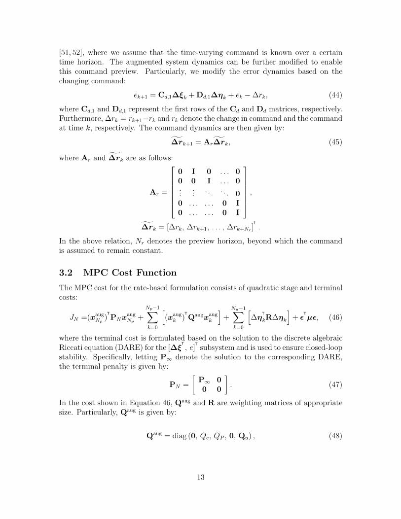
[51, 52], where we assume that the time-varying command is known over a certaintime horizon. The augmented system dynamics can be further modified to enablethis command preview. Particularly, we modify the error dynamics based on thechanging command:

ek+1 = Cd,1∆ξk + Dd,1∆ηk + ek −∆rk, (44)

where Cd,1 and Dd,1 represent the first rows of the Cd and Dd matrices, respectively.Furthermore, ∆rk = rk+1−rk and rk denote the change in command and the commandat time k, respectively. The command dynamics are then given by:

∆rk+1 = Ar∆rk, (45)

where Ar and ∆rk are as follows:

Ar =

0 I 0 . . . 00 0 I . . . 0...

.... . . . . . 0

0 . . . . . . 0 I0 . . . . . . 0 I

,∆rk = [∆rk, ∆rk+1, . . . , ∆rk+Nr ]

T

.

In the above relation, Nr denotes the preview horizon, beyond which the commandis assumed to remain constant.

3.2 MPC Cost Function

The MPC cost for the rate-based formulation consists of quadratic stage and terminalcosts:

JN =(xaugNp

)T

PNxaugNp

+

Np−1∑k=0

[(xaug

k )T

Qaugxaugk

]+

Nu−1∑k=0

[∆η

T

kR∆ηk

]+ ε

T

µε, (46)

where the terminal cost is formulated based on the solution to the discrete algebraicRiccati equation (DARE) for the [∆ξ

T

, e]T

subsystem and is used to ensure closed-loopstability. Specifically, letting P∞ denote the solution to the corresponding DARE,the terminal penalty is given by:

PN =

[P∞ 00 0

]. (47)

In the cost shown in Equation 46, Qaug and R are weighting matrices of appropriatesize. Particularly, Qaug is given by:

Qaug = diag (0, Qe, QP , 0, Qu) , (48)

13

where diag(·, . . . , ·) denotes a block-diagonal matrix structure composed of the argu-ments. Finally, the last term in the cost is used to penalize violation of soft con-straints, where ε is the vector of slack variables (see Section 3.3). Additionally, wenote that the formulation allows for different prediction (Np) and control (Nu) hori-zons to be used. This is done to maintain a low computational cost by using a shortcontrol horizon while ensuring stability with a long prediction horizon. Particularly,when the control horizon is shorter than the prediction horizon, the control inputsremain unchanged beyond the control horizon and the model is simulated with a con-stant control input until the end of the prediction horizon. Therefore, the MPC hasto solve for fewer control actions, which simplifies the optimization.

3.3 MPC Constraints

To ensure the actuator limits are satisfied in operation, we impose the following inputconstraints:

30% ≤ RHan ≤ 100%, 30% ≤ RHca ≤ 100%,

65 C ≤ Tcool,in ≤ 80 C, 60 V ≤ vcm ≤ 240 V,

0.05 A · cm−2 ≤ idens ≤ 1.75 A · cm−2, 0.1 kg · s−1 ≤ mcool ≤ 4 kg · s−1.

The above constraints are motivated by the fuel cell system capabilities. In caseof the current density, we note that the lower bound is used to ensure operationaway from the open-circuit voltage (OCV), which is a known catalyst and membranestressor [18]. The current density upper bound is chosen based on the compressor’scapability to maintain a safe oxygen stoichiometry.

The rates of change of the inputs are also constrained. This is done to accountfor the actuator dynamics that are not explicitly modeled. For instance, the coolanttemperature cannot change instantaneously due to the dynamics associated with theheater and radiator. Therefore, such dynamic limits are taken into account as follows:

|∆RHan| ≤ 10% s−1 × Ts, |∆RHca| ≤ 10% s−1 × Ts,

|∆Tcool,in| ≤ 0.1 C · s−1 × Ts, |∆vcm| ≤ 10 V · s−1 × Ts,

|∆idens| ≤ 0.5 A · cm−2 · s−1 × Ts, |∆mcool| ≤ 0.2 kg · s−2 × Ts.

Note that the above constraints on the actuators are all enforced as hard constraints,i.e., no constraint violation is allowed.

We also consider safety and degradation constraints that are imposed on the dy-namic states or their rates of change, as well as the auxiliary z variables in Equation33. In particular, to ensure membrane durability we enforce:

5 ≤ λCL ≤ 14, 7 ≤ λmb ≤ 14,

|∆λmb| ≤ 1 s−1 × Ts, Tmb ≤ 87 C.

These constraints are imposed to avoid subjecting the membrane to significant hydra-tion and dehydration cycles and inhibit its excessive heating. Furthermore, the rate

14

of change of the membrane hydration is constrained, since it controls the mechanicalstresses in the membrane that can lead to crack initiation or propagation.

The safe operation of the compressor is guaranteed by the following constraints:

40 kRPM ≤ ωcp ≤ 100 kRPM,

zsurge ≤ −0.1, 0.6 ≤ zchoke,

1.5 bar ≤ psm ≤ 3.5 bar.

Moreover, to ensure robust and sufficient supply of reactants to the active sites in theCLs we impose the following limits:

1.5 ≤ StO2 , 1.2 bar ≤ pca ≤ 3.0 bar,

sCL ≤ 0.3, 0.2 V ≤ Ecell ≤ 0.9 V,

where the constraints on StO2 and pca are used to ensure sufficient delivery of oxygento the cathode channels at a high enough pressure and the constraint on sCL and thelower bound for Ecell guarantee sufficient reactant concentration at the Pt surfaces.The upper bound for Ecell is essentially clipping the cell voltage for improved cata-lyst durability [53]. We also note that the hydrogen stoichiometry is assumed to beconstant at 1.5.

Lastly, to avoid excessive heating of the cell, the change in the coolant temperatureis limited:

∆Tcool ≤ 10 C.

The safety and degradation constraints are all imposed as soft constraints with slackvariables (ε) to ensure feasibility of the problem (see Equation 46).

Overall, these constraints ensure safe and reliable operation of the entire fuel cellsystem and are used to extend the useful lifetime of the fuel cell stack. It is thetype of constraints that is of interest in this work rather than the specific numericalbounds used here, as such numerical values can be updated when the fuel cell systemis characterized based on safety and durability considerations.

3.4 MPC Optimization

To formulate the optimization problem we use the batch approach [54], wherein thelinearized dynamics are utilized to describe all future states in terms of the currentstates and future inputs. Following this approach and considering the constraintsdescribed above, we obtain the optimization problem below, which is a quadraticprogram (QP):

minimizeU

JN = UT

HU + 2qTU

subject to GU ≤W + Txaug0

(49)

15

where U is the input vector over the control horizon augmented with the slack vari-ables:

U =[∆η

T

1, . . . ∆ηT

Nu , εT]T. (50)

Derivation of the cost and constraint matrices in the above QP is straightforward andavailable in the literature [54, 55].

3.5 Tuning of MPC Weights and Horizons

The weighting matrices are chosen as follows:

Qe = 50, QP = 10, Qu = diag (0, 2, 0, 0, 5, 0) ,

R = diag (5, 5, 5, 0.05, 1, 2.5) .

These weights are chosen to penalize the tracking error (Qe = 50) and ensure offset-free tracking of the power demand when possible, while minimizing the power con-sumption by auxiliary equipment (QP = 10). Moreover, two of the system inputsare penalized (nonzero elements in Qu). Specifically, since hydrogen consumption isdirectly related to the stack current (assuming constant hydrogen stoichiometry), thecurrent density is penalized with a weight of 5 to minimize the fuel consumption. Inaddition, a small penalty (weight of 2) is imposed on the cathode channel relative hu-midity (RH) to minimize the humidification requirements and explore opportunitiesfor downsizing the humidifier. Only the cathode RH is penalized, since humidifyingthe cathode requires a larger humidifier due to higher air mass flow rates compared tothe hydrogen flow rates in the anode. The rates of change of the inputs are also pe-nalized (R), wherein the weights are chosen based on the scales of the inputs. Lastly,to obtain the terminal penalty, the DARE is solved with R∞ = R and:

Q∞ = diag (0, Qe, QP ) .

Regarding the MPC prediction and control horizons, longer horizons typically im-prove the controller performance while increasing its computational cost [54]. How-ever, the optimal choice of the prediction horizon depends on the particular problem.Here, a relatively long prediction horizon is needed to effectively control the mem-brane hydration state, since it has slow dynamics compared to other system states.However, longer prediction horizons may in fact lead to deteriorated performance withthe current formulation, because the reduced-order model is much simpler than theplant model and requires frequent updates based on the full-state feedback from thefull-order model. Additionally, the MPC uses a linearized version of this simplifiedmodel, whose deviations from the original nonlinear model become more significantover time. The fact that linearization is done about a non-equilibrium point exacer-bates this discrepancy.

To determine a good prediction horizon, a number of numerical experiments wereconducted with the step profile shown in Section 4. Particularly, values of Np = 10to Np = 35 were tested. It was found that a prediction horizon of Np = 20 strikes a

16

good balance between performance and computational cost. The same procedure wasused to determine the control horizon, where horizons between Nu = 4 and Nu = 10were studied and a control horizon of Nu = 5 was found to yield good performancewith minimal computational costs. Therefore, we set Np = 20 and Nu = 5 for thesimulations in Section 4.

3.6 Numerical Implementation

The entire degradation-conscious control framework is implemented in MATLAB.Particularly, the plant model is integrated with the stiff solver ode23t. The reduced-order dynamics are analytically linearized using CasADi [56]. The QP matrices areformulated using in-house MATLAB code and the optimization is solved with theOperator Splitting Quadratic Program (OSQP) solver [57] that uses the alternatingdirection method of multipliers (ADMM) [58]. A tolerance of 10−5 and a maximumnumber of iterations of 1000 are used. When a number of constraints become active,this iteration limit is reached. Nevertheless, our numerical experiments show neg-ligible improvements in performance or constraint satisfaction when the algorithmis allowed to iterate longer to ensure convergence. Therefore, this maximum itera-tion limit was chosen to balance the algorithm convergence with its computationalrequirements. The simulations are run on a computer with a 2.5 GHz processor and16 GB of RAM.

4 Simulation Case Studies

In this section we study the utility of the proposed framework with a variety of powerdemand profiles and discuss the impact of command preview.

4.1 Power Profile with Step Changes in Demand

In the first case study, we consider a power demand profile that consists of severalincreasing and decreasing step changes in the load as shown in Fig. 2. Moreover, theprofile also includes a high power demand that is not feasible for the fuel cell systemconsidered in this work. This infeasible demand is used to illustrate the controller’sability in satisfying the various safety and degradation constraints while pushing thesystem to its limits. As observed in Fig. 2, the controller enables offset-free tracking ofthe power demand, where the net power generated by the system rapidly converges tothe demand level after a step change. However, in some cases the controller responseis slower to ensure the constraints are satisfied.

With regards to the fuel cell conditions, Fig. 2 illustrates that the controller suc-cessfully maintains the membrane hydration within the desired range. Similarly, themembrane temperature is maintained below the critical value, the liquid accumula-tion in the cathode CL is kept below 0.3, and sufficient oxygen delivery is ensured bysustaining the oxygen stoichiometry above 1.5. The figure also shows the compressor

17

Figure 2: Power and system state trajectories for step changes in power demand. Thedashed black lines indicate system constraints. The compressor state trajectories are over-laid on the compressor efficiency map, where the surge and choke constraints are also shown.

efficiency map with the trajectory of compressor model states overlaid. The controllersuccessfully avoids compressor surge and choke and ensures sufficient pressure in thesupply manifold. Moreover, the compressor efficiency is maximized (the efficiency isalways greater than 72%). Lastly, the change in the coolant temperature is controlledto be below 10 C to ensure the system is not overheated. Slight violations of someof the constraints are observed, which are due to the fact that these constraints areimposed as soft constraints to ensure feasibility. In practice, the constraints can bemade tighter, if needed, to ensure safety and longevity are not compromised withsuch slight violations.

The inputs to the fuel cell system generated by the degradation-conscious con-troller are shown in Fig. 3, where the actuation limits are respected. The coolantflow rate and the cathode channel RH are minimized to reduce the auxiliary powerloss and humidification requirements, respectively. Particularly, at higher loads, themembrane is hydrated with ORR product water. It is only at lower current densities

18

Figure 3: System input trajectories and their computation time for arbitrary powerprofile of Fig. 2. The input limits are shown as dashed black lines.

that cathode inlet humidification is deemed necessary to ensure sufficient hydrationof the membrane. Another interesting observation is that after the load is reduced at210 s, the controller builds up pressure in the cathode channel by running the com-pressor faster. This helps to initially compensate for lack of humidification. Once thecathode feed is sufficiently humidified, the compressor speed is reduced to minimizecompressor power consumption.

Fig. 3 also shows the time required to formulate and solve the QP of Equation49, where the computational time is seen to be consistently less than the samplingtime. The computation times shown in the figure also include the time to evaluate theanalytically linearized dynamics and form the QP matrices. Therefore, the problemis efficiently formulated and solved in real time in the hardware used in this study.Nonetheless, since embedded hardware is typically far less powerful than a desktopcomputer, further computational simplifications may be needed in practice.

One approach to reduce the computational burden in practice is to use a longerexecution horizon (Ne), i.e., instead of just using the first move, we can use thefirst few entries in the control sequence generated by the optimizer. The resultsfrom such an approach are shown in Fig 4, where the execution horizon is increasedfrom 1 to 4 steps. We observe a slight deterioration in controller performance withincreasing execution horizon. Particularly, as shown in the insets, the power trackingcapability is slowed down and the ability to recover from constraint violation is slightlyreduced. Nonetheless, such slight deterioration is not expected to have significantimplications in terms of either the system performance or its durability. Therefore,longer execution horizons may be utilized in practice to alleviate the computationalburden further, if needed.

Alternatively, a larger sampling time may be used for time-discretization. How-

19

Figure 4: Effect of increasing execution horizon. The dashed black lines indicatesystem constraints.

ever, we have found that the controller performance is diminished more significantlywith such an approach, because the resulting time-discretized linear dynamics are notable to capture the behavior of the continuous-time system.

4.2 Time-Varying Power Profiles

As a final step in evaluating the capabilities of the proposed degradation-consciouscontrol framework, here we inspect its utility in following time-varying power de-mands, which is a more realistic scenario for automotive applications. In particular,we study several drive cycles in this subsection. To this end, the speed profile ineach cycle is transformed into a power demand profile using a simple vehicle model.The decelerating portions of a speed profile would lead to negative power. However,we limit the minimum power demand to 10 kW here, since we neither consider ahybridization scheme nor a fuel cell start-up shut-down capability in this work.

We start our analysis with the highway section of the US06 drive cycle (US06-HW). The power demand profile is shown in Fig. 5 along with the net power generatedby the fuel cell system. We note that when no load preview is used, the controllerdisplays a lag in following the power demand (Fig. 5(b)). With a preview horizon ofonly 5 steps (equivalent to 0.5 seconds), the power tracking capability is enhanced sig-nificantly at lower loads. Considering recent advances in human driver modeling [59]and the envisioned connected infrastructure of the future [60], it is indeed reasonableto assume a good-quality short command preview is available in real-world scenarios.Nonetheless, the system is not able to follow rapid and significant increases in theload even with the command preview, as seen at around 10 and 165 seconds in Fig.5(a). This is due to the slow response of the fuel cell system and highlights the needfor hybridization in automotive applications.

Fig. 5 also shows two of the most critical conditions, namely, membrane hydra-tion and the oxygen stoichiometry, where it is observed that the respective constraints

20

(a)

(b)

(c)

(d)

Figure 5: Dynamics for power and example constrained variables for US06 highway drivecycle: (a) power dynamics, (b) blown-up version of the power dynamics plot, where theeffectiveness of command preview is observed, (c) membrane hydration, and (d) oxygenstoichiometry. The dashed black lines indicate system constraints.

21

Figure 6: System input trajectories (calculated with a preview of 5 steps) and theircomputation time for US06-HW drive cycle. The input limits are shown as dashedblack lines.

are successfully satisfied both with and without the command preview. However, themembrane hydration state is better maintained above the critical value with the com-mand preview, highlighting the utility of the preview when the load is time-varying.Overall, these results indicate that the proposed framework can successfully followtime-varying power demands, while ensuring safe and enduring system operation, asdetermined by the constraints.

The input profiles for the US06-HW drive cycle calculated by the controller usingthe command preview information are shown in Fig. 6, where the cathode relativehumidity and the coolant flow rate are minimized as before. Additionally, the com-putation times for the control commands are still consistently below the samplingtime.

Finally, the power profiles for four other drive cycles are shown in Fig. 7, illus-trating the controller’s capability in following a variety of power demands. Overall,these results highlight several opportunities in enhancing performance and durabilityof automotive PEM fuel cell systems through model-based control and underline theimportance of complementing material-based solutions with active control strategiesto meet the cost and durability targets for these systems. Successful implementationof this framework in real-world applications requires the knowledge of key fuel cellstressors and proper lifetime indicators. The membrane hydration and its rate ofchange are among the lifetime indicators used in this work. Nonetheless, the frame-work allows for further such indicators to be included as they are discovered throughextensive ongoing degradation studies. Therefore, the proposed framework offers aflexible strategy to meeting the increasing demands for these fuel cell systems andenabling their widespread commercialization.

22

(a)

(b)

(c)

(d)

Figure 7: Power trajectories for different drive cycles: (a) US06, (b) UDDS, (c) FTP75,and (d) HWFET drive cycles.

23

5 Summary and Conclusions

A framework for degradation-conscious control of PEM fuel cell systems is developed.The framework employs LTV-MPC to meet a power demand, while maximizing theoverall system efficiency, ensuring safe operation of the fuel cell system, and extendingits lifetime. The latter two objectives are achieved by enforcing constraints on thecompressor and fuel cell conditions. Particularly, these constraints are based onconsiderations that stem from compressor safety, membrane mechanical durabilityand the durability of the electrocatalyst. Moreover, the system efficiency is maximizedby minimizing the fuel and auxiliary power consumption.

The framework is implemented by first developing a model of the fuel cell systemthat serves as the plant for our simulation-based studies. The plant model is thensimplified to derive a reduced-order controller model for MPC optimization. Thecontroller model is further simplified by linearizing it about the current operatingpoint. This successive linearization enables the use of linear MPC formulations thatlead to significant computational gains. The particular rate-based MPC formulationemployed here allows us to account for actuator dynamics without the need to ex-plicitly model the actuators. Furthermore, it enables constraint enforcement on therate of change of the system states, which can have serious implications for fuel celldurability.

The results indicate that the proposed control framework is able to meet therequested power demand, even for time-varying profiles. Moreover, it ensures satis-faction of durability constraints and is thus expected to contribute to extending thesystem’s lifetime. Lastly, we show that the results are calculated faster than realtime in the computational hardware used in this study and highlight opportunitiesto further reduce computational cost and ensure successful implementation with em-bedded hardware. Therefore, the proposed framework offers a promising approach tocomplement the ongoing research in developing material-based solutions to addressdurability concerns in fuel cell systems.

24

A APPENDIX

A complete list of model variables and parameters is provided in Table A1 belowfor accessibility. The anode and cathode parameters are assumed to be the sameunless noted otherwise. Additional model parameters can be found in earlier work[40]. Similarly, the compressor parameters that are not listed here can be found inreference [16].

Table A1: Nomenclature and parameter list.

Symbol Description [Units] Value/Eq.

State variablescv Water vapor concentration [mol · cm−3] Eq. 1pl Liquid pressure [bar] Eq. 2T Temperature [C] Eq. 3λ Ionomer water content [−] Eq. 4srelax Ionomer relaxation variable [−] Eq. 5θPtO PtO coverage [−] Eq. 7ωcp Compressor speed [RPM] Eq. 10psm Supply manifold pressure [bar] Eq. 11pca Cathode pressure [bar] Eq. 12Outputs and constrained variablesEcell Cell voltage [V] Eq. 8Pnet Net power output [kW] Eq. 16Pfc Power generated by the fuel cell stack [kW] Eq. 9Pcm Power consumed by the compressor [kW] Eq. 14Paux Auxiliary equipment power consumption [kW] Eq. 17Pfrac Fraction of power used for auxiliary equipment [−] Eq. 18zsurge Approximation for compressor surge boundary [−] Eq. 34zchoke Approximation for compressor choke boundary [−] Eq. 35StO2 Oxygen stoichiometry [−] Eq. 13∆Tcool Coolant temperature change [C] Eq. 15Inputs determined by MPCRHan Relative humidity in the anode channel [−] –RHca Relative humidity in the cathode channel [−] –idens Current density [A · cm−2] –Tcool,in Coolant inlet temperature [C] –mcool Coolant flow rate [kg · s−1] –vcm Compressor motor voltage [V] –Constant inputsStH2 Hydrogen stoichiometry [−] 1.5Structural parametersAcool Cooling area [cm2] 280Afc Single cell active area [cm2] 280AT Cathode outlet throttle area [cm2] 17.5

25

dc Compressor blade diameter [cm] 22.86Dh Channel hydraulic diameter [cm] 0.03Jcp Compressor inertia [kg ·m2] 5× 10−5

ncell Number of cells in the stack [−] 380Vsm Supply manifold volume [m3] 0.02Vca Cathode volume [m3] 0.01δ Layer thickness [µm] –δmb Membrane thickness [µm] 20δCL CL thickness [µm] 4.8/5.8 for an/caδMPL MPL thickness [µm] 30δGDL GDL thickness [µm] 160ε Porosity/volume fraction [−] –εCL CL porosity [−] 0.35εMPL MPL porosity [−] 0.45εGDL GDL porosity [−] 0.65Physical constantsF Faraday’s constant [C ·mol−1] 96485Ma,atm Molar mass of atmospheric air [g ·mol−1] 28.9647MH2 Molar mass of hydrogen [g ·mol−1] 2MH2O Molar mass of water [g ·mol−1] 18MN2 Molar mass of nitrogen [g ·mol−1] 28MO2 Molar mass of oxygen [g ·mol−1] 32R Universal gas constant [J ·mol−1 ·K−1] 8.314Physical properties and local variablesCD Cathode outlet discharge coefficient [−] 0.0124Deffi Effective diffusivity of species i [cm2 · s−1] Ref. [40]

EOCV Open-circuit voltage [V] Ref. [40]EPtO Interaction energy for PtO formation [kJ ·mol−1] 10EW Ionomer equivalent weight [g ·mol−1] 1000hconv Heat convection coefficient [W · cm−2 ·K−1] 0.2iref0,an Reference HOR exchange current density [A · cm−2] 0.1

iref0,ca Reference ORR exchange current density [A · cm−2] 1× 10−7

Keffl Liquid effective permeability [cm2] Ref. [40]

kT,CL CL thermal conductivity [W ·m−1 ·K−1] 0.25kT,MPL MPL thermal conductivity [W ·m−1 ·K−1] 0.15kT,GDL GDL thermal conductivity [W ·m−1 ·K−1] 0.4kT,mb Membrane thermal conductivity [W ·m−1 ·K−1] Ref. [40]kPtO Rate constant for PtO formation [s−1] 0.0128kt Motor constant [N ·m ·A−1] 0.0153kv Motor constant [V · rad−1 · s] 0.0153kca,in Cathode orifice constant [kg · s−1 · Pa−1] 3.63× 10−6

Nw,mb Water flux in ionomer phase [mol · cm−2 · s−1] Ref. [40]nv Fitting parameter for diffusivity correction [−] 3ne Fitting parameter for diffusivity correction [−] 2.2Rmb Membrane ionic resistance [Ω · cm2] Ref. [40]

Reff,caCL Cathode CL effective ionic resistance [Ω · cm2] Ref. [40]

26

Relec Total electronic resistance [Ω · cm2] 0.05RT Total heat transport resistance [cm2 ·K ·W−1] Eq. 26Rv Total vapor transport resistance [s · cm−1] Eq. 31Rcm Motor constant [Ω] 0.82Sh Sherwood number [−] 2.693s Liquid saturation [−] Ref. [40]Sv Source term for vapor transport [mol · cm−3 · s−1] Ref. [40]Sl Source term for liquid transport [g · cm−3 · s−1] Ref. [40]ST Source term for heat transport [W · cm−3 ·K−1] Ref. [40]Sλ Source term for ionomer water transport [mol · cm−3 · s−1] Ref. [40]Tcp Compressor outlet temperature [N ·m] Table 1Uc Compressor blade tip speed [m · s−1] Ref. [16]Wi,in Mass flow rate of i into the cathode [kg · s−1] –Wi,out Mass flow rate of i out of the cathode [kg · s−1] –Wi,GDL Mass flow rate of i into the cathode GDL [kg · s−1] –xO2 Oxygen mass fraction in dry air [−] 0.233αan Transfer coefficient for HOR [−] 2αca Transfer coefficient for ORR [−] 0.7αPtO Transfer coefficient for PtO formation [−] 0.5εα Volume fraction of phase α [−] –εg Volume fraction of gas phase [−] (1− s)εεl Volume fraction of liquid phase [−] sεηHOR HOR activation overpotential [V] Ref. [40]ηORR ORR activation overpotential [V] Ref. [40]ηPtO PtO formation overpotential [V] Ref. [40]ηcm Motor mechanical efficiency [−] 98%ηcp Compressor efficiency [V] Ref. [16]γan Reaction order for HOR [−] 0.5γca Reaction order for ORR [−] 0.8γ Ratio of specific heats for air [−] 1.4κres Residual ionomer conductivity [S · cm−1] 0.002 (Ref. [40])κ0 Reference ionomer conductivity [S · cm−1] 0.4 (Ref. [40])λeq Equilibrium ionomer water content [−] Ref. [40]µl Liquid water viscosity [Pa · s] 4.05× 10−4

ϕ Ionomer relaxation parameter [−] 0.35Φ Normalized compressor flow rate, [−] Ref. [16]ρl Liquid phase density [g · cm−3] 0.997ρion Ionomer density [g · cm−3] 1.9(ρcp)g Volumetric heat capacity of gas phase [J · cm−3 ·K−1] 0.00125(ρcp)l Volumetric heat capacity of liquid phase [J · cm−3 ·K−1] 4.2(ρcp)s Volumetric heat capacity of solid phase [J · cm−3 ·K−1] 2σl Liquid water surface tension [N ·m−1] 0.0644τrelax Ionomer relaxation time constant [s] Eq. 6τcm Compressor motor torque [N ·m] Table 1τcp Torque required to drive the compressor [N ·m] Table 1ωca,in Humidity ratio for cathode inlet [−] –

27

Catalyst structural parametersECSA Electrochemically active surface area [(m2 · g−1)Pt] 55/70 for an/caIC Ionomer to carbon ratio [−] 1.1/0.9 for an/caLPt Pt loading [mg · cm−2] 0.15/0.2 for an/cawt% Pt/C weight fraction [−] 0.35Subscripts, superscripts, and abbreviationsad Absorption/desorption –an Anode side –ca Cathode side –cool Coolant –cm Compressor motor –cp Compressor –CH Channel –CL Catalyst layer –g Gas phase –GDL Gas diffusion layer –HOR Hydrogen oxidation reaction –ion Ionomer –l Liquid phase –mb Membrane –MPL Microporous layer –OCV Open-circuit voltage –ORR Oxygen reduction reaction –pc Phase change –sm Supply manifold –v Vapor phase –

References

[1] M. M. Mench, E. C. Kumbur, and T. N. Veziroglu, Polymer electrolyte fuel cell degra-dation. Academic Press, 2011.

[2] C. Gittleman, A. Kongkanand, D. Masten, and W. Gu, “Materials research and devel-opment priorities for low cost automotive PEM fuel cells,” Current Opinion in Elec-trochemistry, 2019.

[3] B. K. Hong, P. Mandal, J.-G. Oh, and S. Litster, “On the impact of water activityon reversal tolerant fuel cell anode performance and durability,” Journal of PowerSources, vol. 328, pp. 280–288, 2016.

[4] P. Mandal, B. K. Hong, J.-G. Oh, and S. Litster, “Understanding the voltage reversalbehavior of automotive fuel cells,” Journal of Power Sources, vol. 397, pp. 397–404,2018.

28

[5] B. Kienitz, J. Kolde, S. Priester, C. Baczkowski, and M. Crum, “Ultra-thin reinforcedionomer membranes to meet next generation fuel cell targets,” ECS Transactions,vol. 41, no. 1, pp. 1521–1530, 2011.

[6] E. Endoh, “Development of highly durable PFSA membrane and MEA for PEMFCunder high temperature and low humidity conditions,” ECS Transactions, vol. 16,no. 2, pp. 1229–1240, 2008.

[7] S. M. Stewart, R. L. Borup, M. S. Wilson, A. Datye, and F. H. Garzon, “Ceria anddoped ceria nanoparticle additives for polymer fuel cell lifetime improvement,” ECSTransactions, vol. 64, no. 3, pp. 403–411, 2014.

[8] A. M. Baker, L. Wang, W. B. Johnson, A. K. Prasad, and S. G. Advani, “Nafionmembranes reinforced with ceria-coated multiwall carbon nanotubes for improved me-chanical and chemical durability in polymer electrolyte membrane fuel cells,” TheJournal of Physical Chemistry C, vol. 118, no. 46, pp. 26796–26802, 2014.

[9] C. Lim, A. S. Alavijeh, M. Lauritzen, J. Kolodziej, S. Knights, and E. Kjeang, “Fuel celldurability enhancement with cerium oxide under combined chemical and mechanicalmembrane degradation,” ECS Electrochemistry Letters, vol. 4, no. 4, pp. F29–F31,2015.

[10] A. Kongkanand and M. F. Mathias, “The priority and challenge of high-power perfor-mance of low-platinum proton-exchange membrane fuel cells,” The journal of physicalchemistry letters, vol. 7, no. 7, pp. 1127–1137, 2016.

[11] G. S. Harzer, J. N. Schwammlein, A. M. Damjanovic, S. Ghosh, and H. A. Gasteiger,“Cathode loading impact on voltage cycling induced PEMFC degradation: A voltageloss analysis,” Journal of The Electrochemical Society, vol. 165, no. 6, pp. F3118–F3131,2018.

[12] R. L. Borup and A. Z. Weber, “FC-PAD: Fuel cell performance and durability consor-tium,” in Annual Merit Review Proceedings, U.S. Department of Energy, 2019.

[13] J. Golbert and D. R. Lewin, “Model-based control of fuel cells::(1) regulatory control,”Journal of power sources, vol. 135, no. 1-2, pp. 135–151, 2004.

[14] J. Golbert and D. R. Lewin, “Model-based control of fuel cells (2): Optimal efficiency,”Journal of power sources, vol. 173, no. 1, pp. 298–309, 2007.

[15] J. T. Pukrushpan, A. G. Stefanopoulou, and H. Peng, “Control of fuel cell breathing,”IEEE Control Systems Magazine, vol. 24, no. 2, pp. 30–46, 2004.

[16] J. T. Pukrushpan, A. G. Stefanopoulou, and H. Peng, Control of fuel cell power sys-tems: principles, modeling, analysis and feedback design. Springer Science & BusinessMedia, 2004.

[17] C. Ziogou, E. N. Pistikopoulos, M. C. Georgiadis, S. Voutetakis, and S. Papadopoulou,“Empowering the performance of advanced NMPC by multiparametric programming– An application to a PEM fuel cell system,” Industrial & Engineering ChemistryResearch, vol. 52, no. 13, pp. 4863–4873, 2013.

29

[18] R. Borup, J. Meyers, B. Pivovar, Y. S. Kim, R. Mukundan, N. Garland, D. Myers,M. Wilson, F. Garzon, D. Wood, et al., “Scientific aspects of polymer electrolyte fuelcell durability and degradation,” Chemical reviews, vol. 107, no. 10, pp. 3904–3951,2007.

[19] F. D. Bianchi, C. Kunusch, C. Ocampo-Martinez, and R. S. Sanchez-Pena, “A gain-scheduled LPV control for oxygen stoichiometry regulation in pem fuel cell systems,”IEEE Transactions on Control Systems Technology, vol. 22, no. 5, pp. 1837–1844, 2013.

[20] J. Sun and I. V. Kolmanovsky, “Load governor for fuel cell oxygen starvation protec-tion: A robust nonlinear reference governor approach,” IEEE Transactions on ControlSystems Technology, vol. 13, no. 6, pp. 911–920, 2005.

[21] A. Vahidi, I. Kolmanovsky, and A. Stefanopoulou, “Constraint management in fuelcells: A fast reference governor approach,” in Proceedings of the 2005, American Con-trol Conference, 2005., pp. 3865–3870, IEEE, 2005.

[22] A. Vahidi, I. Kolmanovsky, and A. Stefanopoulou, “Constraint handling in a fuel cellsystem: A fast reference governor approach,” IEEE Transactions on Control SystemsTechnology, vol. 15, no. 1, pp. 86–98, 2006.

[23] A. Vahidi, A. Stefanopoulou, and H. Peng, “Current management in a hybrid fuel cellpower system: A model-predictive control approach,” IEEE Transactions on ControlSystems Technology, vol. 14, no. 6, pp. 1047–1057, 2006.

[24] A. Vahidi and W. Greenwell, “A decentralized model predictive control approach topower management of a fuel cell-ultracapacitor hybrid,” in 2007 American ControlConference, pp. 5431–5437, IEEE, 2007.

[25] J. Luna, S. Jemei, N. Yousfi-Steiner, A. Husar, M. Serra, and D. Hissel, “Nonlinearpredictive control for durability enhancement and efficiency improvement in a fuel cellpower system,” Journal of Power Sources, vol. 328, pp. 250–261, 2016.

[26] S. Kumaraguru, “Durable high power membrane electrode assembly with low Pt load-ing,” in Annual Merit Review Proceedings, U.S. Department of Energy, 2017.

[27] M. Hasan and M. H. Santare, “Characterizing durability of PFSA membranes of PEMfuel cell based on numerical fatigue crack propagation,” in Meeting Abstracts, no. 34,pp. 1522–1522, The Electrochemical Society, 2019.

[28] M. Hasan, A. Goshtasbi, J. Chen, M. H. Santare, and T. Ersal, “Model-based analysisof PFSA membrane mechanical response to relative humidity and load cycling in PEMfuel cells,” Journal of The Electrochemical Society, vol. 165, no. 6, pp. F3359–F3372,2018.

[29] Y.-H. Lai, K. M. Rahmoeller, J. H. Hurst, R. S. Kukreja, M. Atwan, A. J. Maslyn,and C. S. Gittleman, “Accelerated stress testing of fuel cell membranes subjectedto combined mechanical/chemical stressors and cerium migration,” Journal of TheElectrochemical Society, vol. 165, no. 6, pp. F3217–F3229, 2018.

30

[30] M. A. Danzer, S. J. Wittmann, and E. P. Hofer, “Prevention of fuel cell starvationby model predictive control of pressure, excess ratio, and current,” Journal of PowerSources, vol. 190, no. 1, pp. 86–91, 2009.

[31] C. Hahnel, V. Aul, and J. Horn, “Power control for efficient operation of a PEM fuel cellsystem by nonlinear model predictive control,” IFAC-PapersOnLine, vol. 48, no. 11,pp. 174–179, 2015.

[32] A. Ebadighajari, H. Homayouni, J. DeVaal, and F. Golnaraghi, “Model predictivecontrol of polymer electrolyte membrane fuel cell with dead-end anode and periodicpurging,” in IEEE Conference on Control Applications, pp. 1500–1505, IEEE, 2016.

[33] C. Ziogou, S. Papadopoulou, M. C. Georgiadis, and S. Voutetakis, “On-line nonlinearmodel predictive control of a PEM fuel cell system,” Journal of Process Control, vol. 23,no. 4, pp. 483–492, 2013.

[34] J. Luna, E. Usai, A. Husar, and M. Serra, “Enhancing the efficiency and lifetime ofa proton exchange membrane fuel cell using nonlinear model-predictive control withnonlinear observation,” IEEE transactions on industrial electronics, vol. 64, no. 8,pp. 6649–6659, 2017.

[35] L. Chisci, P. Falugi, and G. Zappa, “Gain-scheduling MPC of nonlinear systems,” In-ternational Journal of Robust and Nonlinear Control: IFAC-Affiliated Journal, vol. 13,no. 3-4, pp. 295–308, 2003.

[36] T. Keviczky and G. J. Balas, “Receding horizon control of an F-16 aircraft: A com-parative study,” Control Engineering Practice, vol. 14, no. 9, pp. 1023–1033, 2006.

[37] P. Falcone, F. Borrelli, H. E. Tseng, J. Asgari, and D. Hrovat, “Linear time-varyingmodel predictive control and its application to active steering systems: Stability analy-sis and experimental validation,” International Journal of Robust and Nonlinear Con-trol: IFAC-Affiliated Journal, vol. 18, no. 8, pp. 862–875, 2008.

[38] A. Goshtasbi, B. L. Pence, and T. Ersal, “Computationally efficient pseudo-2D non-isothermal modeling of polymer electrolyte membrane fuel cells with two-phase phe-nomena,” Journal of The Electrochemical Society, vol. 163, no. 13, pp. F1412–F1432,2016.

[39] A. Goshtasbi, B. L. Pence, and T. Ersal, “A real-time pseudo-2D bi-domain modelof PEM fuel cells for automotive applications,” in ASME 2017 Dynamic Systems andControl Conference, pp. V001T25A001–V001T25A001, American Society of Mechani-cal Engineers, 2017.

[40] A. Goshtasbi, B. L. Pence, J. Chen, M. A. DeBolt, C. Wang, J. R. Waldecker, S. Hirano,and T. Ersal, “A mathematical model toward real-time monitoring of automotive PEMfuel cells,” Journal of The Electrochemical Society, vol. 167, 2020.

[41] A. Goshtasbi, P. Garcıa-Salaberri, J. Chen, K. Talukdar, D. G. Sanchez, and T. Ersal,“Through-the-membrane transient phenomena in PEM fuel cells: A modeling study,”Journal of The Electrochemical Society, vol. 166, no. 7, 2019.

31

[42] N. Subramanian, T. Greszler, J. Zhang, W. Gu, and R. Makharia, “Pt-oxide coverage-dependent oxygen reduction reaction (ORR) kinetics,” Journal of The ElectrochemicalSociety, vol. 159, no. 5, pp. B531–B540, 2012.

[43] G. A. Futter, P. Gazdzicki, K. A. Friedrich, A. Latz, and T. Jahnke, “Physical modelingof polymer-electrolyte membrane fuel cells: Understanding water management andimpedance spectra,” Journal of Power Sources, vol. 391, pp. 148–161, 2018.

[44] L. Hao, K. Moriyama, W. Gu, and C.-Y. Wang, “Modeling and experimental validationof Pt loading and electrode composition effects in PEM fuel cells,” Journal of TheElectrochemical Society, vol. 162, no. 8, pp. F854–F867, 2015.

[45] K. W. Suh, Modeling, analysis and control of fuel cell hybrid power systems. PhDthesis, The University of Michigan, 2006.

[46] N. S. Khattra, Z. Lu, A. M. Karlsson, M. H. Santare, F. C. Busby, and T. Schmiedel,“Time-dependent mechanical response of a composite PFSA membrane,” Journal ofPower Sources, vol. 228, pp. 256–269, 2013.

[47] M. P. Rodgers, L. J. Bonville, H. R. Kunz, D. K. Slattery, and J. M. Fenton, “Fuelcell perfluorinated sulfonic acid membrane degradation correlating accelerated stresstesting and lifetime,” Chemical reviews, vol. 112, no. 11, pp. 6075–6103, 2012.

[48] D. S. Bernstein, Matrix mathematics: theory, facts, and formulas. Princeton UniversityPress, 2009.

[49] G. Pannocchia and J. B. Rawlings, “The velocity algorithm LQR: a survey,” TechnicalReport 2001-01, TWMCC, 2001.

[50] G. Betti, M. Farina, and R. Scattolini, “A robust MPC algorithm for offset-free trackingof constant reference signals,” IEEE Transactions on Automatic Control, vol. 58, no. 9,pp. 2394–2400, 2013.

[51] C. Gohrle, A. Schindler, A. Wagner, and O. Sawodny, “Design and vehicle implementa-tion of preview active suspension controllers,” IEEE Transactions on Control SystemsTechnology, vol. 22, no. 3, pp. 1135–1142, 2013.

[52] S. Di Cairano and I. V. Kolmanovsky, “Automotive applications of model predictivecontrol,” in Handbook of Model Predictive Control, pp. 493–527, Springer, 2019.

[53] J. P. Meyers, “Modeling of catalyst structure degradation in PEM fuel cells,” in Mod-eling and Numerical Simulations, pp. 249–271, Springer, 2008.

[54] F. Borrelli, A. Bemporad, and M. Morari, Predictive control for linear and hybridsystems. Cambridge University Press, 2017.

[55] A. Bemporad, M. Morari, V. Dua, and E. N. Pistikopoulos, “The explicit linearquadratic regulator for constrained systems,” Automatica, vol. 38, no. 1, pp. 3–20,2002.

32

[56] J. A. E. Andersson, J. Gillis, G. Horn, J. B. Rawlings, and M. Diehl, “CasADi –A software framework for nonlinear optimization and optimal control,” MathematicalProgramming Computation, vol. 11, no. 1, pp. 1–36, 2019.

[57] B. Stellato, G. Banjac, P. Goulart, A. Bemporad, and S. Boyd, “OSQP: An operatorsplitting solver for quadratic programs,” ArXiv e-prints, Nov. 2017.

[58] S. Boyd, N. Parikh, E. Chu, B. Peleato, J. Eckstein, et al., “Distributed optimizationand statistical learning via the alternating direction method of multipliers,” Founda-tions and Trends in Machine Learning, vol. 3, no. 1, pp. 1–122, 2011.

[59] M. Albaba, Y. Yildiz, N. Li, I. Kolmanovsky, and A. Girard, “Stochastic driver model-ing and validation with traffic data,” in 2019 American Control Conference, pp. 4198–4203, IEEE, 2019.

[60] A. Sciarretta and A. Vahidi, Energy-Efficient Driving of Road Vehicles: Toward Co-operative, Connected, and Automated Mobility. Springer, 2019.

33