Deformable Model with Adaptive Mesh and Automated Topology Changes

Jacques-Olivier Lachaud Benjamin TatonLaboratoire Bordelais de Recherche en Informatique

351, cours de la Liberation33405 TALENCE CEDEX - FRANCE

Abstract

Due to their general and robust formulation deformablemodels offer a very appealing approach to 3D image seg-mentation. However there is a trade-off between modelgenericity, model accuracy and computational efficiency. Ingeneral, fully generic models require a uniform sampling ofeither the space or their mesh. The segmentation accuracyis thus a global parameter. Recovering small image featuresresults in heavy computational costs whereas generally onlyrestricted parts of images require a high segmentation ac-curacy.This paper presents a highly deformable model that both

handles fully automated topology changes and adapts itsresolution locally according to the geometry of image fea-tures. The main idea is to replace the Euclidean metric witha Riemannian metric that expands interesting parts of theimage. Then, a regular sampling is maintained with thisnew metric. This allows to automatically handle topologychanges while increasing the model resolution locally ac-cording to the geometry of image components. By this wayhigh quality segmentation is achieved with reduced compu-tational costs.

1. Introduction

Deformable models are extensively used in the field ofimage analysis. Their formulation provides a very robustand general framework that remains available in a widerange of applications and many variants have been tailoredto solve efficiently given problems. Since they often use apriori knowledge on the shape and the topology of recov-ered objects these models remain very application specificand are not well suited to general object reconstruction.In contrast, various models achieve extraction of image

components with arbitrary complex topology. That kindof models is of great interest in the field of 3D biomedi-cal image analysis where objects have complex and some-times unexpected shapes, and where accurate initialization

of models is difficult. As a counterpart to their generic-ity these solutions come in general with important increasesof the number of shape parameters and hence of time andspace complexity. Of course segmentation is expected torecover the finest image details. Time and space complexityis thus fully determined by the image resolution and com-putational costs become prohibitive due to the steady im-provements of acquisition devices.

This emphasizes the need for multi-scale approaches.These methods should be able to recover accurately ob-jects with arbitrary topology while keeping a restricted setof shape parameters. The contribution of this paper is topresent an attempt in this direction. The model we proposeis an extension of the model first presented in [7]. It is aclosed oriented triangular mesh designed to reconstruct ob-jects with an arbitrary topology from large 3D images. Ourmodel changes its topology in a fully automated way andhas the ability to adapt its resolution according to the ge-ometry of image features. The computational costs of thesegmentation step and of any subsequent operation are thusreduced, while object shapes remain accurately represented.In addition, our model comes with the usual advantages ofparametric models, namely intuitive user interaction as wellas easy introduction of additional constraints through thedefinition of new forces [3, 15]. Moreover, coarse to fineapproaches remain available.

The first part of the paper recalls significant previousworks that involve topology and resolution adaptation inthe context of 3D image segmentation. The second partdescribes our model and explains how topological changesare detected and handled and how adaptive resolution isachieved by changing metrics. The third part shows howthese metrics are computed directly from images. Experi-mental results are presented and discussed in the last part ofthe paper.

2. Previous works

2.1. Topology adaptation

The various models that achieve adaptive topology areusually classified in two categories.In the parametric approach, objects are represented ex-

plicitly as polygonal meshes. Topological changes are per-formed by applying local reconfigurations to the modelmesh [4, 6, 7] or by computing a new topologically consis-tent parameterization of the model [9]. The main difficultyconsists in detecting self-collisions of the model. McIner-ney and Terzopoulos [9] investigate the intersections of thepolygonal mesh with a simplicial grid that covers the im-age. Then they detect special configurations that character-ize self intersections of the model. Lachaud andMontanvert[7] keep the sampling of their triangulated surface regular.This makes it possible to detect self collisions of the de-formable model by checking distances between non neigh-bor vertices. With an adapted data structure the complexityof this algorithm is where denotes the numberof vertices used to sample the surface.In the level-set approach [2, 8] object boundaries are no

longer described explicitly: they are represented as the zerolevel-set of a mapping defined over the image space. Theboundary evolution is translated into evolution equations in-volving which are solved iteratively to make the modelapproach image contours. With these methods topologi-cal changes do not require additional procedures since theyare embedded in the evolution of . Theoretically has tobe computed on the whole image space, which is compu-tationally expensive. These costs are significantly reducedby updating only in narrow band around the zero level of[1]. This band must however be reset periodically and themethod remains costly.

2.2. Adaptive resolution

This section recalls different extensions to the defor-mable models described in Sect. 2.1 that were proposed toachieve an adaptive resolution.In the framework of level-set the mapping is usually

computed on a regular grid. In the same way, the grid usedby McInerney and Terzopoulos is also regular. To recoverthe finest image features the grid should have the same res-olution as the image. Similarly in [7] automated topologicalchanges are made possible through a uniform sampling ofthe model triangulated surface. The finest image structurescan only be detected if all the mesh triangles have the samedimension as image voxels. All these methods have there-fore heavy computational costs when working with highresolution images.

One way to reduce computation times is to adopt a“coarse to fine” approach. Deformable models are initial-ized with a coarse resolution and then deformed towardtheir energy minimum. Then they are globally refined andtheir energy is minimized again. This process is repeateduntil the expected accuracy is reached. With this methodthe costs of the first deformations are significantly reduced.However algorithms remain expensive when the requestedaccuracy increases. In addition, it is not always possible torecover the image details that are lost or ignored during thefirst steps of the algorithm.In the context of parametric models, an other approach is

to adapt the vertex density on the polygonal mesh depend-ing on the geometric properties of objects. Delingette [5]propose to adapt locally the resolution of simplex meshesaccording to the model curvature. This is achieved in twoways. First, an internal force that attracts vertices towardshighly curved parts of the mesh is introduced. Secondly,faces of the model are checked periodically, and those witha curvature higher than a given threshold are refined. Thevertex number is optimized without spoiling segmentationquality. However, automated topological changes of sim-plex meshes are possible only in the context of -D im-ages [10]: volume image reconstruction requires the helpof a supervisor. In addition, mesh refinement is governedby quantities that are computed from the deformable modelitself and are thus clearly a posteriori information. Asa consequence, vertex number optimization should onlybe performed once an accurate segmentation has been ob-tained. This requires a uniform high resolution of the modelmesh and implies important computational costs. At lastDelingette explains [5] that this method does not performwell on noisy images, since outliers and hence noise tend tobe refined.

3. Model description

3.1. Resolution adaptation

As the model presented in [7], our model keeps a regu-lar sampling. This is achieved by maintaining length con-straints on the deformable surface edges. Namely, for twoneighbor vertices and on the mesh we make sure that

(1)

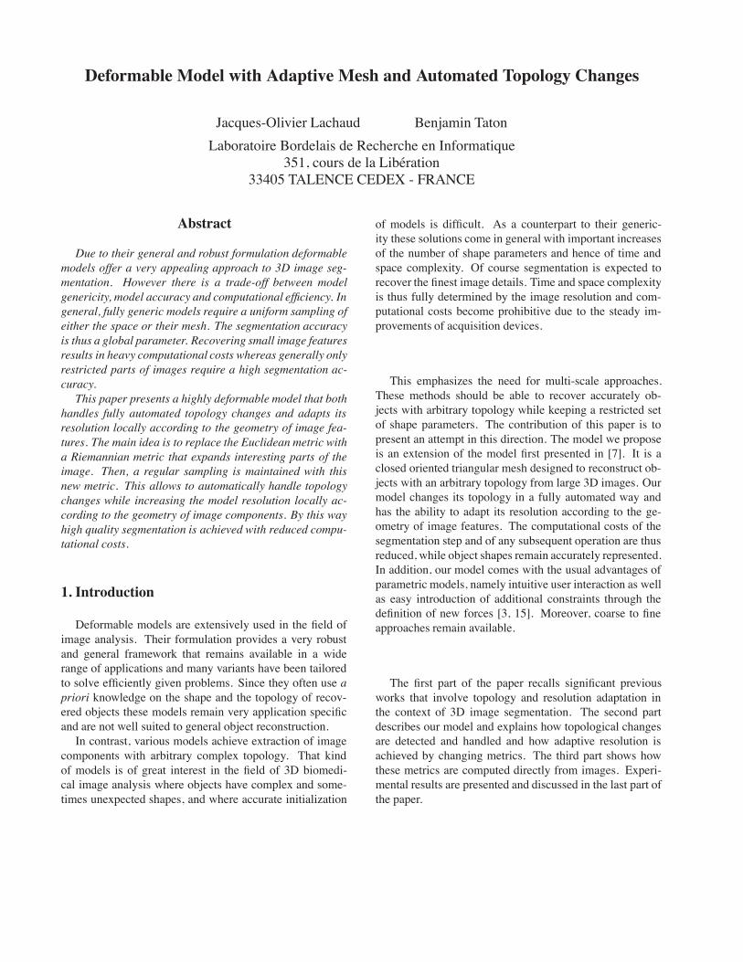
where denotes the Euclidean distance betweenand . The parameter determines the global resolution ofthe model. The parameter determines the ratio betweenthe length of the longest and shortest edges allowed for themodel. After each deformation of the model, each edge ischecked. If one of the constraints no longer holds then theinvestigated edge is either split or contracted as shown onFig 1.

(a) (b) (c)

Figure 1. Operators used to restore the con-straint on edge lengths. ( ) edge inversion,( ) vertex creation, ( ) vertex merge. Trans-formation in ( ) must be handled in a specialway when the two merged vertices share acommon neighbour (see Fig. 3.b).

In [12, 13], the authors consider their mesh as a springmass system. They achieve adaptive resolution by locallychanging the stiffness of the springs according to the fea-tures found in the image. Instead, we propose to leavethe mechanical properties of the system unchanged and tochange the way distances are estimated.Namely, the Euclidean distance is replaced by a Rie-

mannian distance that geometrically expands area of in-terest. Informally speaking, is chosen to overestimatedistances in the vicinity of interesting image features. As aconsequence, the lengths of the model edges tend to over-run the threshold . Therefore edges tend to split (Fig 1.a)and the model mesh gets locally finer. Symmetrically,underestimates distances in areas with no significant imageinformation. Therefore, edge lengths decrease under thethreshold and are contracted (Fig 1.c). This results in alocally coarser resolution.More precisely, a Riemannianmetric is a way to measure

elementary displacements depending on both their originand their orientation. The length of a displacement

starting form is given byin a Euclidean space. In a Riemannian

space, it takes the more general form:

(2)

where denotes a symmetrical positive-definitematrix, namely a dot-product. The mapping should beand is called a Riemannian metric. The geometrical in-

terpretation of metric changes as well as the way metrics arebuilt from images are discussed in detail in Sect. 4.Theoretically, computing exact distances between two

vertices and requires the minimization of the functional

over set of the paths that join and . Namely, it consists infinding and measuring a shortest path (a geodesic) betweenand . However, on the model mesh, neighbor vertices are

close from each other so that may be considered as con-stant along edges. With this assumption the shortest path

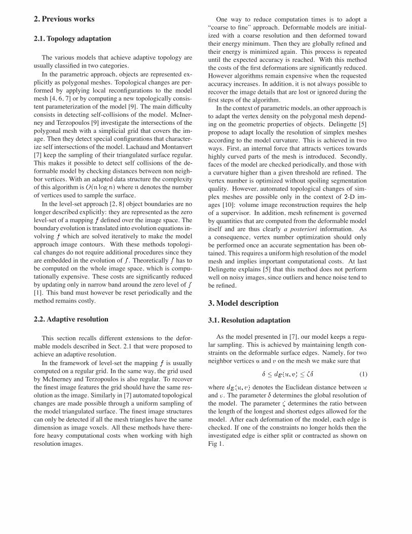
Figure 2. Collision detection method. A ver-tex cannot cross over a face of thedeformable model unless it enters one of thesphere centered in , or with radius .

between and is a straight line the length of which iseasily and efficiently computed.

3.2. Topology adaptation

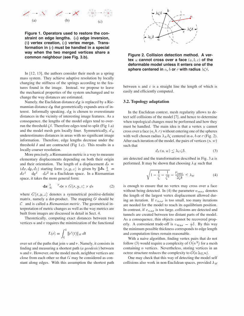
In the Euclidean context, mesh regularity allows to de-tect self collisions of the model [7], and hence to determinewhen topological changes must be performed and how theymust be handled. The main idea is that a vertex cannotcross over a face without entering one of the sphereswith well chosen radius centered in , or (Fig. 2).After each iteration of the model, the pairs of verticessuch that

(3)

are detected and the transformation described in Fig. 3.a isperformed. It may be shown that choosing such that

(4)

is enough to ensure that no vertex may cross over a facewithout being detected. In (4) the parameter denotesthe length of the largest vertex displacement allowed dur-ing an iteration. If is too small, too many iterationsare needed for the model to reach its equilibrium position.In contrast, if is too large, collisions are detected andtunnels are created between too distant parts of the model.As a consequence, thin objects cannot be recovered prop-erly. A convenient trade-off is . By this waythe minimum possible thickness corresponds to edge lengthand computation times remain reasonable.With a naive algorithm, finding vertex pairs that do not

follow (3) would require a complexity of for a meshcontaining vertices. Nevertheless, storing vertices in anoctree structure reduces the complexity to .One may check that this way of detecting the model self

collisions also work in non-Euclidean spaces, provided

( ) ( )

Figure 3. Transforms used to restore the topo-logical consistency of the model. When twoparts of the surface collide the local reconfig-uration of themesh shown in is performed.When a tunnel between two parts of the vol-ume becomes too tight, reconfiguration isperformed.

is replaced with a new constant that takes account of themetric. This results in the following choice

3.3. Dynamics

As most parametric models our deformable surface isviewed as a set of vertices, each of which evolves underthe influence of various forces, namely the usual internalregularizing forces , a damping force, along with anyadditional external force .On a Riemannian manifold, the trajectory of a vertex

submitted to a force is theoretically described by the fol-lowing set of equations:

(5)

where and respectively de-note the vertex mass and position. The coefficients areknown as the Christoffel’s symbols and are given as

where denotes the coefficient at position in thematrix . Compared with the Newton’s laws of motion,equation (5) includes the additional term .Since is and is everywhere positive-definite, the

Christoffels symbols and hence the additional term couldeasily be computed. However this term is second order in. Therefore it has no influence on the deformable modelequilibrium position and is negligible compared to the forcevector which includes the damping force . That is

why this term is not taken into account so that we get backthe usual Newton’s laws

(6)

Experimentally, ignoring the additional term does not in-duce any visible change on the model behavior and signif-icantly reduces computational costs. Equation (6) is classi-cally discretized in time using the finite difference scheme,which allows to iteratively approach the model rest position.

4. Riemannian metrics

This section gives an intuitive geometrical interpretationof metric changes. Then it recalls the definition and proper-ties of structure tensor and explains how this tool is used tobuild metrics from images.

4.1. Geometrical interpretation

This section shows that changing metrics is equivalentto locally expands or contracts the space along directionsand with ratios determined by the local metric eigenstruc-ture. This is seen by oberving that small balls are deformedinto ellipsoids when the Eulidean metric is replaced by aRiemannian metric.Consider the Riemannian ball . For small

enough values of , is contained in a neighbor-hood over which may be considered as constant. Thus thefollowing approximation holds for any point in :

(7)

If denote the coordinates of in an orthonor-mal basis of eigenvectors of , equation (7) isrewritten as

where , and denote the eigenvalues of . This isthe equation of an ellipsoid oriented along , andand with the length of its semi axes given as ,and .As a consequence, changing the Euclidean metric with a

Riemannian metric is equivalent to locally expand or shrinkthe space along the local eigendirections of the new metric.Expansion ratio are given as along , alongand along .

4.2. Metric choice

As explained in Sect 3.1 a regular sampling of the modelmesh is maintained with the deformed metric. In addition,this metric locally expand or contract the space according

to its eigenstructure. As a result resolution is locally multi-plied by , or depending on the relative orien-tation of the mesh and the vectors , and .Classically, deformable models detect high norms of the

image gradient to track object boundaries. In the followingthese places are called contours and are used to determinehow metrics are built.In a place with weak contours, resolution should remain

coarse. This is achieved by choosing

where denotes the minimum allowed metric eigen-value. We choose . By this way the Euclideanlength of the longest edge on the surface is directly given by. The mesh orientation has no importance in this context,the only constraint on , and is thus orthonormality.In contrast, in the vicinity of contours the metric should

reflect their geometrical properties. Let and denotethe contour strength and normal. Let also andand and denote the contour principal directions andcurvatures. With these notations the local metric eigende-composition is chosen as

andandand

where and denote increasing functions of their argu-ments. With these choices, resolution is adapted accordingto the local geometry of object boundaries, the relative posi-tions of the deformable surface and the image contour, andthe confidence we have in this contour (i.e. its strength).When the model crosses over an image contour, the ver-

tex density on its mesh increases. The maximum resolutionis determined by and is reached when the deformablesurface is tangent to (i.e. when it is orthogonal to im-age component boundaries). The model is thus given moredegrees of freedom to adapt its geometry and fit the con-tour. In addition, the thickness of thin flat objects is over-estimated. This prevents collisions from being detected be-tween parts of the model located on both sides of these ob-jects. As a result, thin surfaces are properly recovered whileedges remain significantly longer than the surface thickness.In contrast, on its rest position the model has the same

geometry as the contour so that its principal directionsmatch the metric eigendirections and . As a result, themesh resolution is determined by the curvatures and :resolution remains coarse in both direction along plane con-tours ( ), increases in the direction of onlyalong sharp edges or tubular structures ( ),and increases in both directions in the vicinity of object cor-ners ( ).

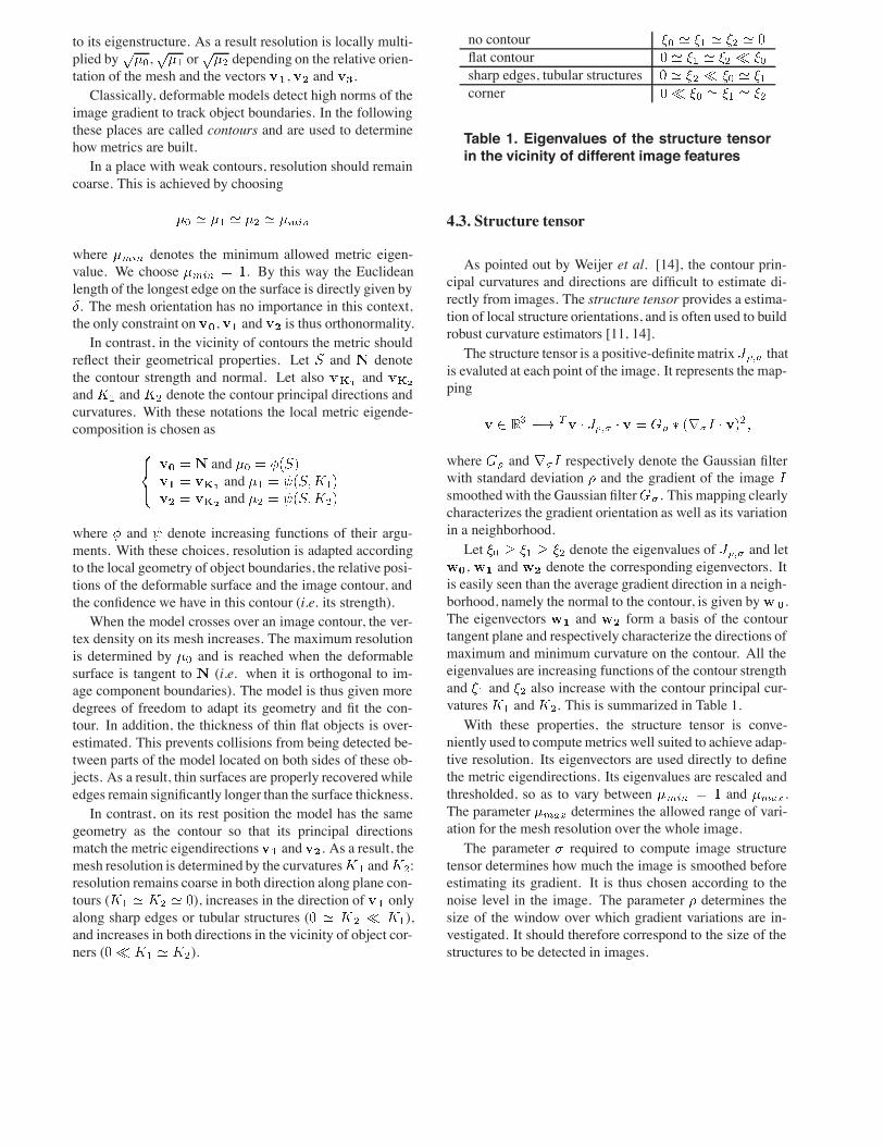
no contourflat contoursharp edges, tubular structurescorner

Table 1. Eigenvalues of the structure tensorin the vicinity of different image features

4.3. Structure tensor

As pointed out by Weijer et al. [14], the contour prin-cipal curvatures and directions are difficult to estimate di-rectly from images. The structure tensor provides a estima-tion of local structure orientations, and is often used to buildrobust curvature estimators [11, 14].The structure tensor is a positive-definitematrix that

is evaluted at each point of the image. It represents the map-ping

where and respectively denote the Gaussian filterwith standard deviation and the gradient of the imagesmoothedwith the Gaussian filter . This mapping clearlycharacterizes the gradient orientation as well as its variationin a neighborhood.Let denote the eigenvalues of and let, and denote the corresponding eigenvectors. It

is easily seen than the average gradient direction in a neigh-borhood, namely the normal to the contour, is given by .The eigenvectors and form a basis of the contourtangent plane and respectively characterize the directions ofmaximum and minimum curvature on the contour. All theeigenvalues are increasing functions of the contour strengthand and also increase with the contour principal cur-vatures and . This is summarized in Table 1.With these properties, the structure tensor is conve-

niently used to compute metrics well suited to achieve adap-tive resolution. Its eigenvectors are used directly to definethe metric eigendirections. Its eigenvalues are rescaled andthresholded, so as to vary between and .The parameter determines the allowed range of vari-ation for the mesh resolution over the whole image.The parameter required to compute image structure

tensor determines how much the image is smoothed beforeestimating its gradient. It is thus chosen according to thenoise level in the image. The parameter determines thesize of the window over which gradient variations are in-vestigated. It should therefore correspond to the size of thestructures to be detected in images.

5. Experimental results

In this section, we investigate and compare segmentationaccuracy and efficiency of (i) our model, (ii) the Euclideanmodel [7] with a fine uniform resolution (iii) the Euclideanmodel with a coarse uniform resolution. From one modelto another only the metric and the edge length (i.e. the pa-rameter in (1)) are changed. The set of forces applied tothe model vertices as well as their balancing are left strictlyidentical for the three models. The mesh resolutions of theEuclideanmodels are chosen so as to correspond to the min-imal andmaximal edge lengths achieved by our Riemannianmodel.For both examples, initialization is performed manualy

outside objects. The model vertices evolve under the actionof the classical regularizing forces, a damping force and ainflation/deflation force that attracts vertices toward a givenimage isosurface. The model is considered to have reachedits rest position when its average kinetic energy stabilizes(see Fig. 5 and Fig. 9).In the first example (Fig. 4-5), the image is composed of

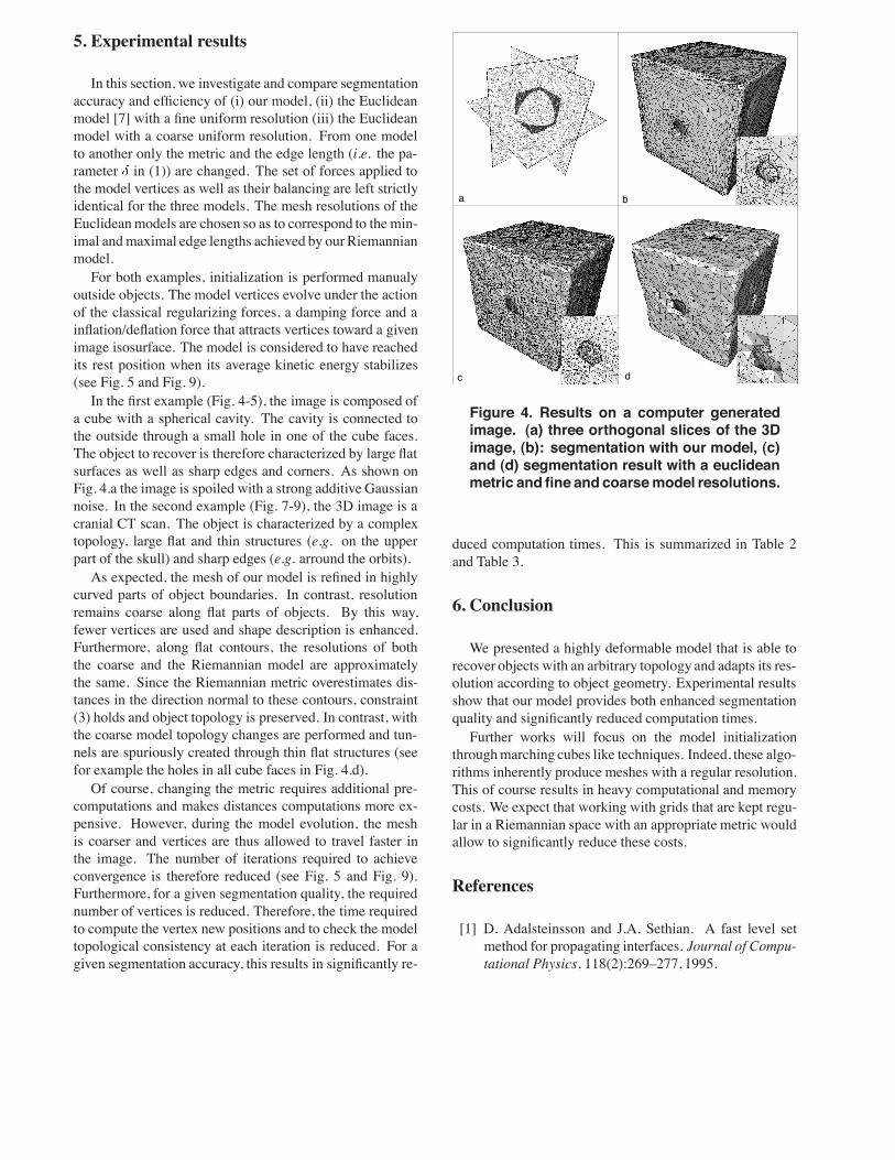
a cube with a spherical cavity. The cavity is connected tothe outside through a small hole in one of the cube faces.The object to recover is therefore characterized by large flatsurfaces as well as sharp edges and corners. As shown onFig. 4.a the image is spoiled with a strong additive Gaussiannoise. In the second example (Fig. 7-9), the 3D image is acranial CT scan. The object is characterized by a complextopology, large flat and thin structures (e.g. on the upperpart of the skull) and sharp edges (e.g. arround the orbits).As expected, the mesh of our model is refined in highly

curved parts of object boundaries. In contrast, resolutionremains coarse along flat parts of objects. By this way,fewer vertices are used and shape description is enhanced.Furthermore, along flat contours, the resolutions of boththe coarse and the Riemannian model are approximatelythe same. Since the Riemannian metric overestimates dis-tances in the direction normal to these contours, constraint(3) holds and object topology is preserved. In contrast, withthe coarse model topology changes are performed and tun-nels are spuriously created through thin flat structures (seefor example the holes in all cube faces in Fig. 4.d).Of course, changing the metric requires additional pre-

computations and makes distances computations more ex-pensive. However, during the model evolution, the meshis coarser and vertices are thus allowed to travel faster inthe image. The number of iterations required to achieveconvergence is therefore reduced (see Fig. 5 and Fig. 9).Furthermore, for a given segmentation quality, the requirednumber of vertices is reduced. Therefore, the time requiredto compute the vertex new positions and to check the modeltopological consistency at each iteration is reduced. For agiven segmentation accuracy, this results in significantly re-

a

d

b

c

Figure 4. Results on a computer generatedimage. (a) three orthogonal slices of the 3Dimage, (b): segmentation with our model, (c)and (d) segmentation result with a euclideanmetric andfine and coarsemodel resolutions.

duced computation times. This is summarized in Table 2and Table 3.

6. Conclusion

We presented a highly deformable model that is able torecover objects with an arbitrary topology and adapts its res-olution according to object geometry. Experimental resultsshow that our model provides both enhanced segmentationquality and significantly reduced computation times.Further works will focus on the model initialization

throughmarching cubes like techniques. Indeed, these algo-rithms inherently produce meshes with a regular resolution.This of course results in heavy computational and memorycosts. We expect that working with grids that are kept regu-lar in a Riemannian space with an appropriate metric wouldallow to significantly reduce these costs.

References

[1] D. Adalsteinsson and J.A. Sethian. A fast level setmethod for propagating interfaces. Journal of Compu-tational Physics, 118(2):269–277, 1995.

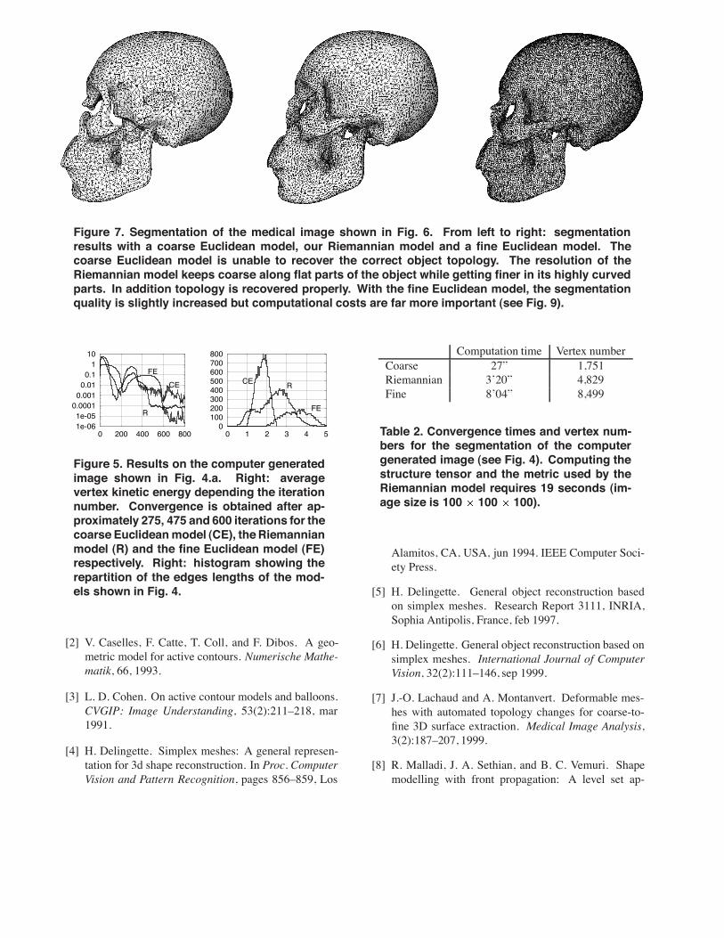
Figure 7. Segmentation of the medical image shown in Fig. 6. From left to right: segmentationresults with a coarse Euclidean model, our Riemannian model and a fine Euclidean model. Thecoarse Euclidean model is unable to recover the correct object topology. The resolution of theRiemannian model keeps coarse along flat parts of the object while getting finer in its highly curvedparts. In addition topology is recovered properly. With the fine Euclidean model, the segmentationquality is slightly increased but computational costs are far more important (see Fig. 9).

1e-061e-050.00010.0010.010.1110

0 200 400 600 800

CE

R

FE

0100200300400500600700800

0 1 2 3 4 5

CE R

FE

Figure 5. Results on the computer generatedimage shown in Fig. 4.a. Right: averagevertex kinetic energy depending the iterationnumber. Convergence is obtained after ap-proximately 275, 475 and 600 iterations for thecoarse Euclideanmodel (CE), theRiemannianmodel (R) and the fine Euclidean model (FE)respectively. Right: histogram showing therepartition of the edges lengths of the mod-els shown in Fig. 4.

[2] V. Caselles, F. Catte, T. Coll, and F. Dibos. A geo-metric model for active contours. Numerische Mathe-matik, 66, 1993.

[3] L. D. Cohen. On active contour models and balloons.CVGIP: Image Understanding, 53(2):211–218, mar1991.

[4] H. Delingette. Simplex meshes: A general represen-tation for 3d shape reconstruction. In Proc. ComputerVision and Pattern Recognition, pages 856–859, Los

Computation time Vertex numberCoarse 27” 1,751Riemannian 3’20” 4,829Fine 8’04” 8,499

Table 2. Convergence times and vertex num-bers for the segmentation of the computergenerated image (see Fig. 4). Computing thestructure tensor and the metric used by theRiemannian model requires 19 seconds (im-age size is 100 100 100).

Alamitos, CA, USA, jun 1994. IEEE Computer Soci-ety Press.

[5] H. Delingette. General object reconstruction basedon simplex meshes. Research Report 3111, INRIA,Sophia Antipolis, France, feb 1997.

[6] H. Delingette. General object reconstruction based onsimplex meshes. International Journal of ComputerVision, 32(2):111–146, sep 1999.

[7] J.-O. Lachaud and A. Montanvert. Deformable mes-hes with automated topology changes for coarse-to-fine 3D surface extraction. Medical Image Analysis,3(2):187–207, 1999.

[8] R. Malladi, J. A. Sethian, and B. C. Vemuri. Shapemodelling with front propagation: A level set ap-

Figure 6. Slices extracted from medical data.Segmentation results are presented in Fig. 7.

Figure 8. Segmentation of the medical imageshown in Fig. 6 with the Riemannian model.Four steps of the model evolution. Themodelget refined only when it approaches interest-ing parts of the image.

proach. IEEE Trans. on Pattern Analysis and MachineIntelligence, 17(2):158–174, feb 1995.

[9] T. McInerney and D. Terzopoulos. Medical image seg-mentation using topologically adaptable surfaces. InJ. Troccaz, E. Grimson, and R. Mosges, editors, Proc.of CVRMed-MRCAS, volume 1205 of LNCS, pages23–32, Grenoble, France, mar 1997. Springer-Verlag.

[10] J. Montagnat, H. Delingette, N. Scapel, and N. Ay-ache. Representation, shape, topology and evolutionof deformable surfaces. application to 3d medical im-age segmentation. Technical Report RR-3954, INRIA,2000.

[11] Bernd Rieger and Lucas J. van Vliet. Curvature of-dimensionnal space curves in gray-value images.

1e-091e-081e-071e-061e-050.00010.001

0 500 1000 1500

CER

FE

010002000300040005000600070008000

0 0.01 0.02 0.03

CER

FE

Figure 9. Results on the biomedical imageshown in Fig. 6. Left: average kinetic en-ergy of the vertices depending on the inter-ation number. Coarse Euclidean model (CE)and Riemannian model (R) require both ap-proximately 750 iterations to converge, whilethe fine Euclidean (FE) model only reaches itsrest position after approximately 1,600 itera-tions. Right: Histogram showing the reparti-tion of the edge lengths of the models shownin Fig. 7.

Computation time Vertex numberCoarse 13’23” 10,876Riemannian 32’38” 19,438Fine 151’26” 68,949

Table 3. Convergence times and vertex num-bers for the segmentation of the head CT(Fig. 7). Structure tensor and metric com-putation over the image requires 59 seconds(image size is 148 148 148).

IEEE Trans. on Image Processing, 11(7):738–745,July 2002.

[12] D. Terzopoulos and M. Vasilescu. Sampling and re-constructionwith adaptivemeshes. InProc. CVPR’91,pages 70–75, Lahaina, jun 1991. IEEE.

[13] M. Vasilescu and D. Terzopoulos. Adaptive meshesand shells. In Proc. CVPR’92, pages 829–832, Cham-pain, jun 1992. IEEE.

[14] Joost von Weijer, Lucas J. van Vliet, and Michaelvan Ginkel. Curvature estimation in oriented patternsusing curvilinear models applied to gradient vectorfields. IEEE Trans. on Pattern Analysis and MachineIntelligence, 23(9):1035–1043, September 2001.

[15] C. Xu and J. L. Prince. Snakes, shapes, and gradi-ent vector flow. IEEE Trans. on Image Processing,7(3):359–369, mar 1998.