Deformable M-Reps for 3D Medical Image...

International Journal of Computer Vision 55(2/3), 85–106, 2003c© 2003 Kluwer Academic Publishers. Manufactured in The Netherlands.

Deformable M-Reps for 3D Medical Image Segmentation

STEPHEN M. PIZER, P. THOMAS FLETCHER, SARANG JOSHI, ANDREW THALL,JAMES Z. CHEN, YONATAN FRIDMAN, DANIEL S. FRITSCH, A. GRAHAM GASH,JOHN M. GLOTZER, MICHAEL R. JIROUTEK, CONGLIN LU, KEITH E. MULLER,

GREGG TRACTON, PAUL YUSHKEVICH AND EDWARD L. CHANEYMedical Image Display & Analysis Group, University of North Carolina, Chapel Hill

Received October 26, 2001; Revised September 13, 2002; Accepted June 27, 2003

Abstract. M-reps (formerly called DSLs) are a multiscale medial means for modeling and rendering 3D solidgeometry. They are particularly well suited to model anatomic objects and in particular to capture prior geometricinformation effectively in deformable models segmentation approaches. The representation is based on figuralmodels, which define objects at coarse scale by a hierarchy of figures—each figure generally a slab representinga solid region and its boundary simultaneously. This paper focuses on the use of single figure models to segmentobjects of relatively simple structure.

A single figure is a sheet of medial atoms, which is interpolated from the model formed by a net, i.e., a mesh orchain, of medial atoms (hence the name m-reps), each atom modeling a solid region via not only a position and awidth but also a local figural frame giving figural directions and an object angle between opposing, correspondingpositions on the boundary implied by the m-rep. The special capability of an m-rep is to provide spatial and orien-tational correspondence between an object in two different states of deformation. This ability is central to effectivemeasurement of both geometric typicality and geometry to image match, the two terms of the objective functionoptimized in segmentation by deformable models. The other ability of m-reps central to effective segmentation istheir ability to support segmentation at multiple levels of scale, with successively finer precision. Objects modeledby single figures are segmented first by a similarity transform augmented by object elongation, then by adjustmentof each medial atom, and finally by displacing a dense sampling of the m-rep implied boundary. While these modelsand approaches also exist in 2D, we focus on 3D objects.

The segmentation of the kidney from CT and the hippocampus from MRI serve as the major examples in thispaper. The accuracy of segmentation as compared to manual, slice-by-slice segmentation is reported.

Keywords: segmentation, medial, deformable model, object, shape, medical image

1. Introduction

Segmentation via deformable models has shown theadvantage of allowing the expected geometric con-formation of objects to be expressed (Cootes, 1993;Staib, 1996; Delingette, 1999; among others, also seeMcInerny, 1996 for a survey of active surfaces meth-ods). The basic formulation is to represent an object bya set of geometric primitives and to deform the objectby changing the values of the primitives to optimize anobjective function including a match of the deformed

object to the image data. Either the objective functionalso includes a term reflecting the geometric typical-ity of the deformed object, or the deformation is con-strained to objects with adequate geometric typicality.In our work the objective function is the sum of a geo-metric typicality term and a geometry to image matchterm.

The most common geometric representation in theliterature of segmentation by deformable models hasbeen a mesh of boundary locations. The hypothesisdescribed and tested in this paper is that improved

86 Pizer et al.

• • •

•

Figure 1. A 2D illustration of (left) the traditional view of the me-dial locus of an object as a sheet of disks (spheres in 3D) bitangentto the object boundary and our equivalent view (right) as an m-rep:a curve (sheet in 3D) of hubs at the sphere center and equal lengthspokes normal to object boundary. The locus of the spoke ends formsthe medially implied boundary.

segmentations will result from using a representationthat is at multiple levels of scale and that at all but thefinest levels of scale is made from meshes of medialatoms. We will show that this geometric representa-tion, which we call m-reps, has advantages in measur-ing both the geometric typicality and the geometry toimage match, in providing the efficiency advantages ofsegmentation at multiple scales, and in characterizingthe object as an easily deformable solid.

Many authors, in image analysis, geometry, humanvision, computer graphics, and mechanical modeling,have come to the understanding, originally promul-gated by Blum (1967), that the medial relationship1

between points on opposite sides of a figure (Fig. 1) isan important factor in the object’s geometric descrip-tion. Biederman (1987), Marr (1978), Burbeck (1996),Leyton (1992), Lee (1995), and others have producedpsychophysical and neurophysiological evidence forthe importance of medial relationships (in 2D projec-tion) in human vision. The relation has also been ex-plored in 3D by Nackman (1985), Vermeer (1994),and Siddiqi (1999), and medial axis modeling tech-niques have been applied by many researchers, includ-ing Bloomenthal (1991), Wyvill (1986), Singh (1998),Amenta (1998), Bittar (1995), Igarashi (1999) andMarkosian (1999). Of these, Bloomenthal and Wyvillprovided skeletal-based soft-objects; Singh providedmedial (wire-based) deformations; Amenta and Bittarworked on medially based reconstruction; Igarashiused a medial spine in 2D to generate 3D surfacesfrom sketched outlines; and Markosian used implicitsurfaces generated by skeletal polyhedra.

One of the advantages of a medial representationis that it allows one to distinguish object deforma-tions into along-object deviations, namely elongationsand bendings, and across-object deviations, namelybulgings and attachment of protrusions or indentations.

An additional advantage is that distances, and thus spa-tial tolerances, can be expressed as a fraction of medialwidth. These properties allow positions and orienta-tions to be followed through deformations of elonga-tion, widening, or bending. Because geometric typi-cality requires comparison of corresponding positionsof an object before and after deformation and becausegeometry to image match requires comparison of inten-sities at corresponding positions, this ability to providewhat we call a figural coordinate system is advanta-geous in segmentation by deformable models.

Medial representations divide a multi-object com-plex into objects and objects into figures, i.e., slabs withan unbranching medial locus (see Fig. 1). In the fol-lowing we also show how they naturally divide figuresinto figural sections, and how by implying a bound-ary they aid in dividing the boundaries of these fig-ural sections into smaller boundary tiles. This natu-ral subdivision into the very units of medical interestprovides the opportunity for segmentation at multiplelevels of scale, from large scale to small, that pro-vides at each scale a segmentation that is of smallertolerance than the previous, just larger scale. Such ahierarchical approach was promulgated by Grenander(1981). Such a multi-scale-level approach is requiredfor a segmentation that operates in time linear in thenumber of the smallest scale geometric elements, herethe boundary tiles. The fact that at each level the unitsare geometrically related to the units of relatively uni-form tissue properties yields effective and efficientsegmentations.

Our m-reps representation described in Pizer (1999)and Joshi (2001) (in the first reference called DSLs)reverses the notion of medial relations descended fromBlum (1967) from a boundary implying a medial de-scription to a mesh of medial atoms implying bound-aries, i.e., from an unstable to a stable relation. Theradius-proportional ruler and the need to have localityat the scale of the figural section require it to use awidth-proportional sampling of the medial surface inplace of a continuous medial sheet.2 These latter prop-erties follow from the desire directly to represent shape,i.e., object geometry of some locality that is similaritytransform invariant. The specifics are given later in thissection.

M-reps also extend the medial description to theinclusion of a width-proportional tolerance, provid-ing opportunities for stages of the representation withsuccessively smaller tolerances. Representations withlarge tolerance can ignore detail and focus on gross

Deformable M-Reps for 3D Medical Image Segmentation 87

Figure 2. M-reps: In the 2D example (left) there are 4 figures: a main figure, a protrusion, an indentation, and a separate object. Each figureis represented by a chain of medial atoms. Certain medial atoms in a subfigure are interfigurally linked (dashed lines on the left) to their parentfigures. In the 3D example of a hippocampus (middle) there is one figure, represented by a mesh of medial atoms. Each hub with two linesegment spokes forms a medial atom (Fig. 3). The mesh is viewed from two directions, and the renderings below show the boundary implied bythe mesh. The example on the right shows a 4-figure m-rep for a cerebral ventricle.

shape, and in these large-tolerance stages discretesamplings can be coarse, resulting in considerable ef-ficiency of manipulation and presentation. Smaller-tolerance stages can focus on refinements of the larger-tolerance stages and thus more local aspects.

As described in Pizer (1999) and Joshi (2001), asa result of the aforementioned requirements an m-repmodel of an object is a representation (data structure)consisting of a hierarchy of linked m-rep models forsingle figures (Fig. 2). A model for a single figure ismade from a net (mesh or chain) of medial atoms (hencethe name m-reps), each atom (Fig. 3) designating notonly a medial position x and width r , but also a lo-cal figural frame F implying figural directions, and theobject’s local narrowing rate, given by an object angleθ between opposing, corresponding positions on theimplied boundary. In addition, width proportionalityconstants indicate net link length, boundary tolerance,boundary curvature limits, and, for measuring the fit ofthe atom to a 3D image, an image interrogation aper-ture. As detailed in later papers, a multifigure modelof an object consists of a directed acyclic graph of fig-ure nets, with interfigural links capturing informationabout subfigural location along the parent figure’s me-dially implied boundary, figural width relative to theparent figure, and subfigural orientation relative to theparent figure. The elements of the figural graph alsocontain boundary displacement maps that can be usedto give fine scale to the model.

Sometimes one wishes to represent and then seg-ment multiple disconnected objects at the same time.An example is the cerebral ventricles, hippocampus,and caudate in which the structures are related but one

Figure 3. Medial atoms, made from a position x and two equallength boundary-pointing arrows �p and �s (for “port” and “star-board”), which we call “spokes”. The atom on the left is for aninternal mesh position, implying two boundary sections. The atomon the right is for a mesh edge position, implying a section of bound-ary crest. The atoms are shown in the “atom-plane” containing x,�p and �s. An atom is represented by the medial hub position x; thelength r of the boundary-pointing arrows; a frame made from theunit-length bisector �b of �p and �s, the �b-orthogonal unit vector �n inthe atom plane, and the complementary unit vector �b⊥; and the “ob-ject angle” θ between �b and each spoke. For a slab-like section offigure, �p and �s provide links between the medial point and the im-plied boundary (shown as a narrow curve), giving approximations,with tolerance, to both its position and its normal. The implied figuresection is slab-like and centered on the head of the atom’s spokes,i.e., it is extended in the �b⊥ direction just as it is illustrated to do inthe atom-plane directions perpendicular to its spoke.

88 Pizer et al.

is not a protrusion or an indentation on another. An-other example are the pair of kidneys and the liver. Inour system these can be connected by one or more con-nections between the representations of the respectiveobjects, allowing the position of one figure to predictboundary positions of the other. This matter is left to apaper covering the segmentation of multi-object com-plexes (Fletcher, 2002).

In the remainder of this paper we first (Section 2.1)detail the m-reps data structure and geometry, then(Section 2.2) describe how a continuous boundaryand medial sheets are interpolated from the sampledsheet directly represented in an m-reps figure, and then(Section 2.3) detail the way in which the m-rep pro-vides positional and orientational correspondences be-tween models and deformed models. After brief discus-sions in Sections 2.4 of model building from segmentedobjects that serve for model training, in Section 3 wediscuss the method of segmentation by deformablem-reps. In Section 4 we give results of segmentation ofkidneys, hippocampi, and a horn of the cerebral ven-tricle by these methods, and in Section 5 we concludewith a comparative discussion of our method and indi-cations of future directions in which our segmentationmethod is being developed.

2. Representation of Objects by M-reps

2.1. M-reps Geometry

Intuitively a figure is a main component of an objector a protrusion, an indentation, a hole, or an associatednearby or internally contained object. In Pizer (1999)we carefully define a figure, making it clear that the no-tion is centered on the association of opposing pointson the figure called by Blum (1967) “medial involutes.”Whereas Blum conceived of starting from a boundaryrepresentation and deriving the medial involutes, ouridea is to start with a representation giving medial in-formation and thus widths, and imply sections of fig-ure bounded by involutional regions. As illustrated inFig. 3, in order for a medial atom m by itself to implytwo opposing sections of boundary, as well as the solidregion between them, we define m = {x, r , F, θ} toconsist of

(1) a position, x, the skeletal, or “hub,” position (thisrequires 3 scalars for a 3D atom). x gives the centrallocation of the solid section of figure that is beingrepresented by the atom.

(2) a width, r , the distance from the skeletal position totwo or more implied boundary positions (1 scalar)and thus the length of both �p and �s. r gives thescale of the solid section of figure that is beingrepresented by the atom. That is, it provides a localruler for the object.

(3) a frame F = (�n, �b, �b⊥), implying the tangent planeto the skeleton, via its normal �n, and �b, the partic-ular unit vector in that tangent plane that is alongthe direction of fastest narrowing between the im-plied boundary sections. The medial position x andthe two boundary-pointing arrows, as illustratedin Fig. 3, are in the (�n, �b) plane. The continuousmedial surface implied by the set of m must passthrough each x and have a normal of �n there. Frequires 3 scalars for a 3D atom. F gives the ori-entation of the solid section of figure that is beingrepresented by the atom. That is, it provides a lo-cal figural compass for the object. The frame isgiven by first derivatives of x and r with respect todistance along the tangent plane to x.

(4) an “object angle” θ that determines the angulationof the implied sections of boundary relative to �b�b is rotated by ±θ towards �n to produce normals�p/r and �s/ to the implied boundary. θ is normallybetween π/3 and π/2, the angle corresponding toparallel implied boundaries.

In 3D, figures are generically slabs, though m-reps canalso represent tubes. A slab figure is a 2-sheet of me-dial atoms satisfying the constraint that the impliedboundary folds nowhere. The constraint expresses therelation that the Jacobian of the mapping between themedial surface and the boundary is everywhere pos-itive. A more complete, mathematical presentation ofthe constraints of representations of which legal m-repsare a subset can be found in Damon (2002).

In our representation a discrete m-rep for a slab isa mesh {mij, 1 ≤ i ≤ m, 1 ≤ j ≤ n} of medialatoms that sample a 2-sheet of medial atoms (Fig. 2).We presently use rectangular meshes of atoms (quad-meshes), even though creating and displaying m-repsbased on meshes of triangles (tri-meshes) have advan-tages because of their relation to simplices. In slab fig-ures the net is a two-dimensional mesh and internalnodes of the mesh have a pair of boundary-pointingvectors pointing from x to x + �p and x + �s.

Implied by the atoms in the mesh are

(1) a tolerance τ = βλr of boundary position normalto the boundary,


(2) the length of links to other primitives, approxi-mately of length γ λr , with γ λ significant fractionof 1.0, and

(3) a constraint δλr on the radius of curvature of theboundary.

(4) a size ιλr of the image region whose intensity val-ues directly affect the atom when measuring thematch of the geometric model to the image.

The constant λ specifies the scale of the figural repre-sentation, which will vary from stage to stage in analgorithm working among coarse and fine levels ofrepresentation. The proportionality constants β, γ , δ,and ι are presently set by experience (Burbeck, 1996;Fritsch, 1997; McAuliffe, 1996), and, to maintain mag-nification invariance, the constants βλ, γ λ, δλ, and ιλ

decrease in proportion as the scale decreases.The successive refinement, coarse-to-fine, of a me-

dial mesh can provide a successive correction to themedially implied object by interpolating atoms at thefiner spacing from those at the coarser spacing andthen optimizing the finer mesh (Yushkevich, 2001), al-though we have not implemented this feature yet in them-rep models used in segmentation. This refinementbrings with it a decrease in tolerance of the impliedboundary and radius of curvature constraint, the ad-dition of patches of medial deformations relative to afigural (u, v) space (see Section 2.2) to handle heavilybent sections of slab, as well as proportionately smallerconstant of radius proportionality, λ.

We call a figure represented via m-reps an m-figure.The net of medial atoms contains internal nodes andend nodes, as well. The end nodes for a slab are linkedtogether to form the boundary of the mesh. For an ob-ject made from a single figure, the end nodes needto capture how the boundary of the slab or tube isclosed by what is called a crest in differential geometry(Koenderink, 1990). For example, a pancake is closedat its sides by such a crest. Whereas the internal nodesfor a slab-like segment have two boundary-pointingvectors, end nodes for slab-like segments have threeboundary-pointing vectors, with the additional vectorpointing from x in the �b direction to the crest. Thus �bmust cycle as one moves around the figural crest. Inter-nal nodes for tubes have a circle of boundary-pointingvectors, obtained by adding to x the full circle of rota-tions in a full circle of �p about �b.

For slabs a sequence of edge atoms forms a curveof a crest or a curve of a corner closing the slab. Asillustrated in Fig. 3, these segment closed ends may be

rounded with any level of elongation η: the vertex istaken at x + ηr �b, and the end section in the principaldirection across the implied crest is described by aninterpolation using the position and tangent there andat the two points x+ �p and x+�s and applying an inter-polating function to produce a boundary crest with thedesired extent, tangency, and curvature properties. Weuse this formulation for ends of end atoms representedas {x, r , F, θ, η}, instead of the Blum formulation, inwhich η = 1, in order to stabilize the image match atends as well as to allow corners, i.e., crests of infinitecurvature, to have a finitely sampled representation. Al-though corners do not normally appear in medical im-ages, they are needed to model manufactured objects.Corner atoms have their vertex at x + r (1/ cos(θ ))�b.

2.2. Interpolated Medial Sheetsand Figural Rendering

As stated above, an m-rep mesh of medial atoms fora single figure should be thought of as a represen-tation for a continuous sheet of atoms and a cor-responding continuous implied boundary. The sheetextends to the space curve of points osculating thecrest of the implied figural boundary. We interpo-late the m-rep mesh into this sheet parameterized by(u, v) ∈ [( j, j + 1) × (k, k + 1)] for the mesh elementwith the jkth atom at its lower left corner. The inter-polation is obtained by a process that has local supporton these mesh elements and on the edge elements thatare bounded by edge atoms only. If the medial atomsare separated by constant r -proportional distances, thisparametrization satisfies the objective of representingshape locally.

The interpolation is achieved by applying a variantof subdivision surface methods (Catmull, 1978) to themesh of implied boundary positions and normals givenat the spoke ends (including the crest spokes). The vari-ant, described in detail in Thall (2003), makes the sub-division surface match the position and the normal ofthe spoke ends to within their tolerance. This bound-ary surface (see Fig. 4) is C2 smooth everywhere butthe isolated points corresponding to the atoms at thecorners of the mesh. From this surface Thall’s methodallows the calculation of interpolated medial atoms.

As it stands, Thall’s method is unlikely to producefolded boundaries but is not guaranteed against folds.In our segmentation we penalize against the high cur-vatures that are precursors to a deformation that yieldsfolds. The full avoidance of medial atoms that imply

90 Pizer et al.

Figure 4. Left: A single-figure m-rep. Left middle: Coarse mesh of atom boundary positions for a figure. Right middle: Atom ends vs.interpolated boundary. Right: interpolated boundary mesh at voxel spacing.

a folded boundary will be achievable using the mathe-matical results found in Damon (2002).

The result of Thall’s interpolation is that with eachboundary position we can associate a boundary figuralcoordinate (Pizer, 2002) (Fig. 2), the figure numbertogether with a side parameter t (= −1 for port, = +1for starboard, with t ∈ (−1, 1) around the crest) and theparameters (u, v), describing which interpolated atom’sspoke touches the boundary there. For each figure weinterpolate the atoms sufficiently finely that a set ofvoxel-size triangular tiles represent the boundary. Themethod computes the boundary position and associatednormal and r value for an arbitrary boundary figuralcoordinate (u, v, t).

Points (x, y, z) in space can also be given a figuralcoordinate by appending an r -proportional distance τ

(Fig. 1) to the figural coordinates of the closest me-dially implied boundary point. To allow the distinc-tion by the sign of the distance of the inside and theoutside of the figure, we take the distance to be rela-tive to the medially implied boundary and to be neg-ative on the interior of the figure. A procedure map-ping arbitrary spatial positions (x, y, z) into figuralcoordinates (u, v, t, τ ) has been written. Also, an ar-bitrary fine triangular tiling of the medially impliedboundary can be computed. Rendering can be basedon these triangular tiles or on implicit rendering using

Figure 5. Correspondence over deformation via figural correspondence.

the τ function. As well, the correspondence under fig-ural deformation given by figural coordinates is criti-cally useful in computing the objective function used insegmentation.

2.3. Correspondence Through Deformation

As previously described, figures are designed to pro-vide a natural coordinate system, giving, first a positionon the medial sheet, second a figural side, and finally afigural distance in figural width relative terms along theappropriate medial spoke from a specified position. Asdetailed in Section 3.3, this figural coordinate systemis used in our segmentation method to follow boundarylocations and other spatial locations through the modeldeformation process.

In particular, as illustrated in Fig. 5, a boundary pointafter deformation, identified by its figural coordinatecan be compared to the corresponding point beforedeformation, and the magnitude of the r -proportionaldistance between these points can be used to measurethe local deformation. Also, the intensity in the tar-get image, at a figural coordinate relative to a puta-tively deformed model can be compared to the intensityin a training image (or training images) at the corre-sponding figural coordinate relative to the undeformedmodel.


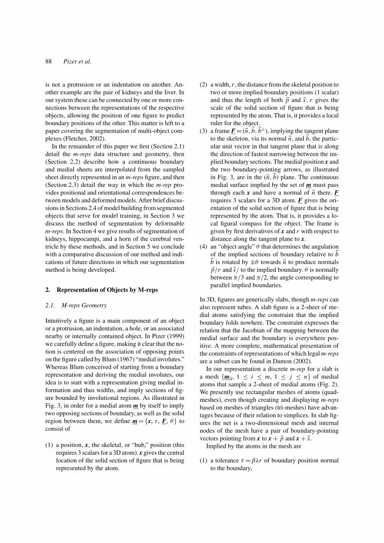
Figure 6. M-reps models. Heavy dots show hubs of medial atoms. Lines are atoms’ spokes. The mesh connecting the medial atoms is shown asdotted curves. Implied boundaries are rendered with shading. Hippocampus: see Fig. 2. Left: kidney parenchyma + renal pelvis. Middle: lateralhorn of cerebral ventricle. Right: multiple single-figure objects in male pelvis: rectum, prostate, bladder, and pubic bones (one bone is occludedin this view).

2.4. M-reps Model Building for Anatomic Objectsfrom Training Images

Model-building must specify of which figures an objector multi-object complex is made up, the size of the meshof each figure, and the way the figures are related, andit must also specify each medial atom. In this paper,focused on single-figure objects, only the mesh sizeand its medial atoms must be specified. Illustrated inthe panels of Fig. 6 are single-figure m-rep models ofa variety of anatomic structures that we have built.

Because an m-rep is intended to allow the repre-sentation of a whole population of an anatomic objectacross patients, it is best to build it based on a significantsample of instances of the segmented object. Styner(2001) describes a tool for stably producing modelsfrom such samples. The hippocampus model shown inFig. 2 was built using this tool. We also have a designtool for building m-rep models from a single training3D-intensity data set and a b-rep from a previous seg-mentation, e.g., a manual segmentation, of the objectin that image. The kidney model shown in Fig. 6 wasbuilt using this tool.

It is obvious that effective segmentation depends onbuilding a model that can easily deform into any in-stance of the object that can appear in a target image.However, the production of models is not the subjectof this paper, so we assume in the following that a sat-isfactory model can be produced and test this fact viathe success of segmentations.

3. Segmentation by Deformable M-reps

3.1. Visualizations

3.1.1. Viewing an M-rep. To allow appreciation ofthe object represented by an m-rep, the m-rep and theimplied boundary must be viewable. To judge if an

m-rep adequately matches the associated image, capa-bilities described in Sections 3.2 and 3.3 are neededto visualize the m-rep in 3D relative to the associatedimage. If the match is not good, the user needs a tool tomodify the m-rep, either as a whole or atom by chosenatom, while in real time seeing the change in the im-plied boundary and the relation of the whole m-rep ormodified atom to the image. After this seldom requiredmanual modification the m-rep or atom may then beattracted by the image data.

As seen in Figs. 2, 4, and 6, we view an m-rep as aconnected mesh of balls, with each ball attached to apair of spokes and, for end atoms, to the crest-pointingηr �b vector. The inter-atom lines, the spokes, and thecrest-pointing vectors can be optionally turned off.In addition, the implied boundary can be viewed as adot cloud, a mesh of choosable density, or a renderedsurface.

3.1.2. Visualization of the M-rep vs. a Target Image.Visualization of greyscale image data must be in 2D;only in 2D image cuts can the human understand the in-teraction of a geometric entity with the image data. Theimplied boundary of an m-rep can be visualized in 3Dversus one or more of the cardinal tri-orthogonal planes(x, y; y, z; or x, z), with the choice of these planes dy-namically changeable (Fig. 11). Other image planes inwhich it is useful to visualize the fit of the m-rep to theimage data are the atom-based planes described in thenext paragraph. Showing the curve of intersection ofthe m-rep implied boundary with any of these imageplanes is useful.

The desired relationship of a single medial atom tothe image data is that at each spoke end there is in theimage a boundary orthogonal to the spoke. This rela-tion is normally not viewable in a cardinal plane. In-stead one needs to visualize and edit the atoms in crosssections of the object that are normal to the boundary.

92 Pizer et al.

Figure 7. The viewing planes of interest for a medial atom: Top: 3D views. Bottom: 2D views.

The spokes of a medial atom, if they have beencorrectly placed relative to the image, are normal tothe perceived boundary, so they should be contained inthe cross section. We conclude that a natural view planeshould contain both of the boundary pointing arrows ofthe medial atom, that is the plane passing through x ofthe atom and spanned by (�n, �b) of the atom (if the objectangle is other than π /2). We call this the atom plane.We can superimpose the medial atom, as well as themedially implied boundary slice on the image in thisplane (Figs. 7(a), (b), and (c)) and visualize in-planechanges in the atom and the boundary there.

On the other hand, the atom may be misplaced or-thogonal to the atom plane or misrotated out of the atomplane, so it needs to be viewed in an image plane or-thogonal to the atom plane. There is no such plane thatcontains both spokes, but if we could live with havingonly one spoke in the atom-orthogonal plane, we couldview across the boundary to which the spoke shouldbe orthogonal. The desired plane is that spanned by theatom’s �b⊥ and the chosen spoke of the atom. But wewould only need the half plane ending at x, the “port” or“starboard half-plane.” Thus, we could draw simulta-neously the two adjoining half planes for the respectivespokes (Fig. 7).

When an atom is selected, it implies visualizationplanes, which can been chosen from among the atomplane, the port spoke half-plane, and the starboard

spoke half-plane. The image data in the chosen plane(s)can be viewed in the 3D viewing window, with the im-age data texture rendered onto these planes (Fig. 7(a)and (b)), and in respective 2D windows for the chosenplane(s) (Figs. 7(c), (d) and (e)).

Manual editing of m-reps, should it be necessary,can be done using these visualizations. The viewer canpoint to positions in the three 2D viewing windowswhere the spoke ends should be moved, and the atomcan be modified to as closely as possible meet theserequirements, based on the object being locally a lin-ear slab. Also, tools for manually rotating, translating,scaling, and changing the object angle and elongation(for end atoms) are easily provided.

3.2. Multi-Scale-Level Model Deformation Strategyfor Segmentation from Target Images

Our method for deforming m-reps into image data al-lows model-directed segmentation of objects in volumedata. The deformation begins with a manually choseninitial similarity transform of the model. To meet theefficiency requirements of accurate segmentation, thesegmentation process then follows a number of stagesof segmentation at successively smaller levels of scale(see Table 1). At each scale level the model is theresult of the next larger scale level and we optimize


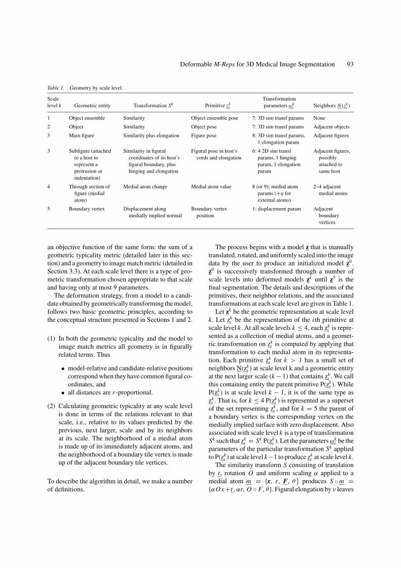
Table 1. Geometry by scale level.

Scale Transformationlevel k Geometric entity Transformation Sk Primitive zk

i parameters ωki Neighbors N (zk

i )

1 Object ensemble Similarity Object ensemble pose 7: 3D sim transf params None

2 Object Similarity Object pose 7: 3D sim transf params Adjacent objects

3 Main figure Similarity plus elongation Figure pose 8: 3D sim transf params,1 elongation param

Adjacent figures

3 Subfigure (attachedto a host torepresent aprotrusion orindentation)

Similarity in figuralcoordinates of its host’sfigural boundary, plushinging and elongation

Figural pose in host’scords and elongation

6: 4 2D sim transfparams, 1 hingingparam, 1 elongationparam

Adjacent figures,possiblyattached tosame host

4 Through section offigure (medialatom)

Medial atom change Medial atom value 8 (or 9): medial atomparams (+η forexternal atoms)

2–4 adjacentmedial atoms

5 Boundary vertex Displacement alongmedially implied normal

Boundary vertexposition

1: displacement param Adjacentboundaryvertices

an objective function of the same form: the sum of ageometric typicality metric (detailed later in this sec-tion) and a geometry to image match metric (detailed inSection 3.3). At each scale level there is a type of geo-metric transformation chosen appropriate to that scaleand having only at most 9 parameters.

The deformation strategy, from a model to a candi-date obtained by geometrically transforming the model,follows two basic geometric principles, according tothe conceptual structure presented in Sections 1 and 2.

(1) In both the geometric typicality and the model toimage match metrics all geometry is in figurallyrelated terms. Thus

• model-relative and candidate-relative positionscorrespond when they have common figural co-ordinates, and

• all distances are r -proportional.

(2) Calculating geometric typicality at any scale levelis done in terms of the relations relevant to thatscale, i.e., relative to its values predicted by theprevious, next larger, scale and by its neighborsat its scale. The neighborhood of a medial atomis made up of its immediately adjacent atoms, andthe neighborhood of a boundary tile vertex is madeup of the adjacent boundary tile vertices.

To describe the algorithm in detail, we make a numberof definitions.

The process begins with a model z that is manuallytranslated, rotated, and uniformly scaled into the imagedata by the user to produce an initialized model z0.z0 is successively transformed through a number ofscale levels into deformed models zk until z5 is thefinal segmentation. The details and descriptions of theprimitives, their neighbor relations, and the associatedtransformations at each scale level are given in Table 1.

Let zk be the geometric representation at scale levelk. Let zk

i be the representation of the i th primitive atscale level k. At all scale levels k ≤ 4, each zk

i is repre-sented as a collection of medial atoms, and a geomet-ric transformation on zk

i is computed by applying thattransformation to each medial atom in its representa-tion. Each primitive zk

i for k > 1 has a small set ofneighbors N(zk

i ) at scale level k and a geometric entityat the next larger scale (k − 1) that contains zk

i . We callthis containing entity the parent primitive P(zk

i ). WhileP(zk

i ) is at scale level k − 1, it is of the same type aszk

i . That is, for k ≤ 4 P(zki ) is represented as a superset

of the set representing zki , and for k = 5 the parent of

a boundary vertex is the corresponding vertex on themedially implied surface with zero displacement. Alsoassociated with scale level k is a type of transformationSk such that zk

i = Sk P(zki ). Let the parameters ωk

i be theparameters of the particular transformation Sk appliedto P(zk

i ) at scale level k−1 to produce zki at scale level k.

The similarity transform S consisting of translationby t , rotation O and uniform scaling α applied to amedial atom m = {x, r , F, θ} produces S ◦ m ={αOx+t, αr, O ◦ F, θ}. Figural elongation by ν leaves

94 Pizer et al.

fixed the medial atoms at a specified atom row i (thehinge end for subfigures) and successively producestranslations and rotations of the remaining atoms interms of the atoms in the previously treated, adjacentrow i−, as follows:

S3(ν) ◦ mi j = {xi− j + ν(xi j − xi− j ), ri j ,

(Fi j F−1

i− j

)ν

◦ Fi− j , θi j}

The subfigure transformation applies a similarity trans-form to each of the atoms in the hinge. This transfor-mation, however, is not in Euclidean coordinates butin the figural coordinates of the boundary of the par-ent. That transformation is not used in this paper, so itsdetails are left to Liu (2002). The medial atom trans-formation S4 translation by t , rotation O , r scaling α,and object angle change �θ applied to a medial atomm = {x, r , F, θ} produces S4(t, O, α, �θ ) ◦ m ={x + t, αr, O ◦ F, θ + �θ}. The boundary displace-ment transformation τ applied to a boundary vertexwith position y, medial radial width r , and mediallyimplied normal �n yields the position y + τr �n.

The algorithm for segmentation successively modi-fies zk−1 to produce zk . In doing so it passes through thevarious primitives zk

i in zk and for each i optimizes anobjective function H(zk , zk−1, I) = wk(-Geomdiff(zk ,zk−1)) + Match(zk , I). Geomdiff(zk , zk−1) measures thegeometric difference between zk and zk−1, and thereby-Geomdiff(zk , zk−1) measures the geometric typicalityof zk at scale level k. Match(zk , I) measures the matchbetween the geometric description zk and the targetimage I. Both Geomdiff(zk , zk−1), and Match(zk , I) aremeasured in reference to the object boundaries Bk andBk−1, respectively implied by zk and zk−1. The weightwk of the geometric typicality is chosen by the user.

For any medial representation z, the boundary B iscomputed as a mesh of quadrilateral tiles as follows,with each boundary tile vertex being known both withregards to its figural coordinates u and its Euclideancoordinates y. For a particular figure, u = (u, v, t),as described in Section 2.2. When one figure is an at-tached subfigure of a host figure, with the attachmentalong the v coordinate of the subfigure, there is a blendregion whose boundary has coordinates u = (u, w, t),where u and t are the figural coordinates of the subfig-ure and w ∈ [−1, 1] moves along the blend from thecurve on the subfigure terminating the blend (w = −1)to the curve on the host figure terminating the blend(w = +1). This blending procedure is detailed in Liu(2002).

As mentioned in Section 2.2, the computation ofB is accomplished by a variation of Catmull-Clarksubdivision (Catmull, 1978) of the mesh of quadrilat-eral tiles (or, in general, tiles formed by any polygon)formed from the two (or three, spoke ends of the medialatoms in z. Thall’s variation (2003) produces a limit sur-face that iteratively approaches a surface interpolatingin position to spoke ends and with a normal interpo-lating the respective spoke vectors. That surface is aB-spline at all but finitely many points on the surface.The program gives control of the number of iterationsand of a tolerance on the normal and thus of the close-ness of the interpolations. A method for extending thisapproach to the blend region between two subfiguresis presently under evaluation.

Geomdiff(zk , zk−1) is computed as the sum of twoterms, one term measuring the difference between theboundary implied by zk and the boundary implied byzk−1, and, in situations when N(zk

i ) is not empty, an-other term measuring the difference between boundaryimplied by zk and that implied by zk with zk

i replacedby its prediction from its neighbors, with the predic-tion based on neighbor relations in P(zk

i ). The secondterm enforces a local shape consistency with the modeland depends on the fact that figural geometry allows ageometric primitive to be known in the coordinate sys-tem of a neighboring primitive. The weight betweenthe neighbor term and the parent term in the geomet-rical typicality measure is set by the user. In the testsdescribed in Section 4, the neighbor term weight was0.0 in the medial atom stage and 1.0 in the boundarydisplacement stage.

The prediction of the value of one geometric prim-itive zk

j in an m-rep from another zki at the same scale

level using the transformation Sk is defined as follows.Choose the parameters of Sk such that Sk applied tothe zk subset of zk−1 is close as possible to zk in thevicinity of zk

j . Apply that Sk to zk to give predictions(Sk zk) j . Those predictions depend on the predictionof one medial atom by another. Medial atom z4

j = {x j ,r j , F j , θ j} predicts medial atom z4

i = {xi , ri , Fi , θi}by recording T = {(x j − xi )/r j , (r j − r j )/r j , F j F

−1i ,

θ j − θi}, where F j F−1i is the rotation that takes frame

Fi into F j . T takes z4i into z4

j and when applied to amodified z4

i produces a predicted z4j .

The boundary difference Bdiff(z1, z2) between twom-reps z1 and z2 is given by the following averager -proportional distance between boundary points thatcorrespond according to their figural coordinates, al-though it could involve points with common figural


coordinates other than at the boundary and it will inthe future involve probabilistic rather than geometricdistance measures.

Bdiff(z1, z2) =[−

∫B2

∥∥y1− y

2

∥∥2

2(σr (y2))2

d y

]/area(B2).

The r -value is that given by the model at the presentscale level, i.e., the parent of the primitive being trans-formed. The normalization of distance by medial radiusr makes the comparison invariant to uniform scaling ofboth the model and the deformed model for the localgeometric component being adjusted at that scale level.

Finally, the geometry to image match measureMatch (zk , I) between the geometric description zk

and the target image I is given by∫ τmax

−τmax

∫Bk G(τ )

Itemplate(y, τ ) I (y′, τ ) d ydτ where y and y′ are bound-ary points in B(zk) and B(zk

template) that agree in figuralcoordinates, G(τ ) is a Gaussian in τ , I is the targetimage I rms-normalized with Gaussian weighting inthe boundary-centered collar τ ∈ [−τmax, τmax] for thedeformed model candidate (see Fig. 8), and the tem-plate image Itemplate and the associated model ztemplate

are discussed in Section 3.3.1.In summary, for a full segmentation of a multi-object

complex, there is first a similarity transformation of thewhole complex, then a similarity transform of each ob-ject, then for each of the figures in turn (with parentfigures optimized before subfigures) first a similarity-like transform that for protrusion and indentationfigures respects their being on the surface of their par-ent, then modification of all parameters of each medialatom. After all of these transformations are complete,there is finally the optimization of the dense boundary

Figure 8. The collar forming the mask for measuring geometry to image match. Left: in 2D, both before and after deformation. Right: in 3D,showing the boundary as a mesh and showing three cross-sections of the collar.

vertices implied by the medial stages. Since in this pa-per we describe only the segmentation of single figureobjects, there are three stages beyond the initialization:the figural stage, the medial atom (figural section)stage, and the boundary displacement stage.

For all of the stages with multiple primitives (in thecase tested in this paper, the medial atom stage andthe boundary stage), we follow the strategy of iterativeconditional modes, so the algorithm cycles among theatoms in the figure or boundary in random order untilthe group converges. The geometric transformation ofa boundary vertex modifies only its position along itsnormal [1 parameter]; the normal direction changes asa result of the shift, thus affecting the next iteration ofthe boundary transformation.

3.3. The Optimization Methodand Objective Function

Multiscale segmentation by deformable models re-quires many applications of optimization of the objec-tive function. The optimization must be done at manyscale levels and for increasingly many geometric prim-itives as the scale becomes smaller. Efficient optimiza-tion is thus necessary. We have tried both evolutionaryapproaches and a conjugate gradient approach to opti-mization. The significant speed advantages of the con-jugate gradient method are utilizable if one can makethe objective function void of nonglobal optima for therange of the parameters being adjusted that is guaran-teed by the previous scale level. We have thus designedour objective functions to have as broad optima as pos-sible and chosen the fineness of our scale levels andintra-level stages to guarantee that each stage or level

96 Pizer et al.

produces a result within the bump-free breadth of themain optimum of the next stage or level.

When the target image is noisy and the object con-trast is low, the interstep fineness requirement justlaid out requires multiple substages of image blurringwithin a scale level. That is, at the first substage thetarget image must be first blurred before being used inthe geometry to image match term. At later substagesthe blurring that is used decreases.

At present the largest scale level involved in a seg-mentation requires a single user-selected weight, be-tween the geometric typicality term and the geometryto image match term. All smaller scale stages requiretwo user-selected weights, the one just mentioned plusa weight between the parent-to-candidate distance andthe neighbor-predictions-to-candidate distance. How-ever, we intend in the future that our objective func-tion be a log posterior probability. When this comesto pass, both terms in the objective function will beprobabilistic, as determined by a set of training im-ages. These terms then would be a log prior for thegeometric typicality term and a log likelihood for thegeometry to image match term. In this situation thereis no issue weighting the geometric typicality and ge-ometry to image match terms. However, at present ourgeometric typicality term is measured in r -proportionalsquared distances from model-predicted positions andthe geometry to image match term is measured in rms-proportional intensity squared units resulting from thecorrelation of a template image and the target image,normalized by local variability in these image intensi-ties. While this strategy allows the objective functionto change little with image intensity scaling or withgeometric scaling, it leaves the necessity of setting therelative weight between the geometric typicality termand the geometry to image match term.

The remainder of this section consists of a subsec-tion detailing the geometry-to-image match term of theobjective function, followed by a section detailing theboundary displacement stage of the optimization.

3.3.1. The Geometry-to-Image Match Measure. It isuseful to compute the match between geometry and theimage based on a model template. Such a match is en-abled by comparing the template image Itemplate and thetarget image data I at corresponding positions in fig-ural coordinates, at figural coordinates determined inthe model. The template is presently determined froma single training image Itemplate, in which the model zhas been deformed to produce ztemplate by applying the

m-reps deformation method through the medial atomscale level (level 4) on the characteristic image corre-sponding to a user-approved segmentation. In our im-plementation the template is defined only in a maskregion defined by a set of figural coordinates, eachwith a weight of a Gaussian in its figural distance-to-boundary, τ , about the model-implied boundary. Thestandard deviation of the Gaussian used for the resultsin this paper is 1/2 of the half-width of the collar. Themask is choosable as a collar symmetrically placedabout the boundary up to a user-chosen multiple of rfrom the boundary (Fig. 8) or as the union of the objectinterior with the collar, a possibility especially easilyallowed by a medial representation. In the results re-ported here we use a boundary collar mask. The mask ischosen by subdividing the boundary positions affectedby the transformation with a fixed mesh of figural co-ordinates (u, v) and then choosing spatial positions tobe spaced along each medial spoke (implied boundarynormal) at that (u, v). These along-spoke positions areequally spaced in the figural distance coordinate τ up toa plus or minus a fixed cutoff value τmax chosen at mod-eling time. For the kidney results reported in Section 4,this cutoff value was 0.3, so the standard deviation ofthe weighting Gaussian in the intensity correlation is0.15.

The template to image match measure is choosablein our tool from among a normalized correlation mea-sure, with weights, and a mutual information measure,with weights, but for all the examples here the cor-relation measure has been used and the weight in allmask voxels is unity. The correlation measure that weuse is an average, over the boundary sample points, ofthe along spoke intensity profile correlations at thesesample points. For the geometry to correspond to thevolume integral of these point-to-corresponding-pointcorrelations, each profile must be weighted by theboundary surface area between it and its neighboringsample points, and the profile must be weighted by itsr -proportional length. In addition, as indicated above,we weight each product in the correlation by a Gaus-sian in τ from the boundary. Also, to make the intensityprofiles insensitive to offsets and linear compression inthe intensity scale, the template is offset to a meanof zero and both the template and the target image arerms-normalized. The template’s rms value is computedwithin the mask in the training image, and the targetimage’s rms value is computed for a region correspond-ing to a blurred version of the mask after the manualplacement of the model.


In our segmentation program the template is choos-able from among a derivative of Gaussian, describedmore precisely below, and the intensity values in thetraining image in the region, described in more detailin Section 4.2. In each case the template is normalizedby being offset by the mean intensity in the mask andnormalized in rms value.

The derivative of Gaussian template for model to im-age match is built in figural coordinates in the space ofthe model, i.e., the space of the training image. Thatis, each along-spoke template profile, after the Gaus-sian mask weighting, is a derivative of a Gaussian witha fixed standard deviation in the figural coordinate τ ,or equivalently an r -proportional standard deviation inEuclidean distance. We choose 0.1 as the value of thestandard deviation in τ . Since this template is associ-ated with the target image via common figural coordi-nates, in effect the template in the target image space isnot a derivative of 3D Gaussian but a warped derivativeof 3D Gaussian, with the template’s standard deviationin spatial terms increases with the figural width.

3.3.2. Boundary Displacement Optimization. Theboundary deformation stage is much like active sur-faces, except that the geometric typicality term consistsnot only of a term measuring the closeness of eachboundary displacement to that at each of the neigh-boring boundary positions but also a term measuringthe log probability of these displacements in the me-dially based prior. Since the tolerance of the mediallyimplied boundary is r -proportional, the log Gaussianmedially based prior, conditional on the medial es-timate, is proportional to the negative square of ther -normalized distance to the medially implied bound-ary (Chen, 1999). The method of Joshi (2001), withwhich we complete the segmentation, uses this com-bined geometric typicality measure, and its boundary toimage match measure is a log probability based on theobject and its background each having normal intensitydistributions.

Figure 9. Segmentation results of the lateral horn of a cerebral ventricle at the m-rep level of scale (i.e., before boundary displacement) fromMRI using a single figure model.

4. Segmentation Results: Deformed Models

4.1. Segmenting the Kidney from CT;Segmentation Accuracy

We have tested this method for the extraction ofthree anatomic objects well modeled by a sin-gle figure: the lateral cerebral ventricle, the kidneyparenchyma + pelvis, and the hippocampus. Extract-ing the lateral ventricle from MR images is not verychallenging because the ventricle appears with highcontrast, but a single result using a Gaussian derivativetemplate is shown in Fig. 9.

Extracting the kidney from CT images is challengingunder the conditions of the work reported here for ra-diation therapy treatment planning (RTP). The kidneysits in a crowded soft tissue environment where partsof its boundary have good contrast resolution againstsurrounding structures but other parts have poor con-trast resolution. Also, not too far away are ribs andvertebrae, appearing very light with very high contrast(Fig. 10). The typical CT protocol for RTP involvesnon-gated slice-based imaging, without breath hold-ing and without injecting the patient with a “dye” toenhance the contrast of the kidney. During the timeinterval between slice acquisition the kidneys are dis-placed by respiratory motion, resulting in significantlyjagged contours in planes tilted relative to the sliceplane (Fig. 10). A combination of partial volume andmotion artifacts causes the poles to be poorly visual-ized or spuriously extended to adjacent slices. Motionand partial volume artifacts degrade the already poorcontrast between the kidney and adrenal gland, whichsits on top of the kidney.

The single figure m-rep used here includes part ofthe pelvis along with the kidney parenchyma, mimick-ing segmentation as performed for RTP. The complexarchitecture of the renal pelvis acts as structure noisefor this m-rep. When using a Gaussian template that isdesigned to give increased response at boundaries next

98 Pizer et al.

Figure 10. Sagittal plane through a CT of the kidney, used in thisstudy, demonstrating significant partial volume and breathing ar-tifacts. A human segmentation is shown as a green tint. Note thescalloped boundary and spurious sections of the kidney, which weresegmented by one of two human raters but excluded by m-rep seg-mentation. Note also the nearby high-contrast rib that can create arepulsive force when a Gaussian derivative template is used.

to which are non-narrow strips of object with intensitylighter than its background, the following behaviors arenoted. (1) If the geometric penalty weight is low, thekidney m-rep can move inside a sequence of vertebralbodies because the high contrast on only a portion ofthe model results in a high model to image match value.

Table 2. Comparison of m-reps segmentation to manual segmentation for six examples selected from 24 kidneys (twelve kidneypairs). Distances are in cm. The examples span the range, from best to worst, of human-m-rep volume overlap.

Kidney code Volumes compared Vol. Overlap 1st-Qtl∗ 2nd-Qtl∗ 3rd-Qtl∗ 〈Dist〉 Haussdorf distance

639 R A–B 0.947 0.000 0.200 0.200 0.117 0.693

A–C 0.940 0.000 0.000 0.200 0.124 1.342

B–C 0.940 0.000 0.200 0.200 0.123 1.183

646 L A–B 0.935 0.000 0.200 0.200 0.133 1.149

A–C 0.939 0.000 0.000 0.200 0.108 0.917

B–C 0.940 0.000 0.000 0.200 0.103 1.077

634 L A–B 0.953 0.000 0.000 0.200 0.103 0.600

A–C 0.903 0.000 0.200 0.200 0.182 0.894

B–C 0.899 0.200 0.200 0.283 0.191 0.849

633 L A–B 0.951 0.000 0.000 0.200 0.106 0.721

A–C 0.909 0.000 0.200 0.200 0.162 1.217

B–C 0.896 0.000 0.200 0.283 0.189 1.131

637 R A–B 0.957 0.000 0.000 0.200 0.079 0.566

A–C 0.843 0.000 0.200 0.400 0.272 1.789

B–C 0.840 0.000 0.200 0.400 0.280 1.897

635 L A–B 0.950 0.000 0.000 0.200 0.097 0.800

A–C 0.807 0.000 0.200 0.400 0.307 2.209

B–C 0.808 0.000 0.200 0.400 0.314 2.272

∗Quartile columns give the surface separation associated with each quartile, e.g., an entry of.200 in the 2nd-Qtl column means that50% of all voxels on the surfaces of the compared segmentations are separated by no more than .200 cm. (.200 cm is the smallestunit of measurement). 〈Dist〉 is the median distance between the surfaces of the compared segmentations.

This is easily prevented by an adequately high weightfor geometric typicality. (2) A portion of the impliedboundary of the kidney m-rep can move to include arib, as a result of the high contrast of the rib. (3) Aportion of the implied boundary of the kidney m-repcan move to include part of the muscle. (4) The bound-ary at the liver, appearing with at most texture contrast,does not attract the implied m-rep boundary, with theresult that the geometric typicality term makes the kid-ney not quite follow the kidney/liver boundary. In otherorgans, parts of the edge with high contrast of oppositepolarity to other parts would repel the m-rep boundary.Avoiding some of these difficulties necessitated replac-ing the first post-initialization similarity transform bya similarity transform augmented by an elongation forthe main figure. Despite these challenges, segmentationusing a Gaussian derivative template, built on a singleright kidney, is successful when compared against hu-man performance.

An example deformation sequence is shown inFig. 11, showing the improved segmentation at eachstage. Results of a typical kidney segmentation arevisualized in Fig. 12. Comparisons between m-repsegmentation (rater C) and human segmentation


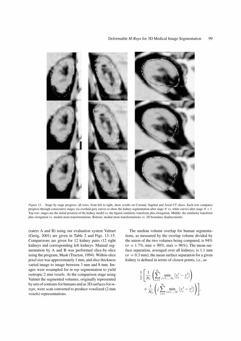
Figure 11. Stage by stage progress: all rows, from left to right, show results on Coronal, Sagittal and Axial CT slices. Each row comparesprogress through consecutive stages via overlaid grey curves to show the kidney segmentation after stage N vs. white curves after stage N + 1.Top row: stages are the initial position of the kidney model vs. the figural similarity transform plus elongation. Middle: the similarity transformplus elongation vs. medial atom transformations. Bottom: medial atom transformations vs. 3D boundary displacements.

(raters A and B) using our evaluation system Valmet(Gerig, 2001) are given in Table 2 and Figs. 13–15.Comparisons are given for 12 kidney pairs (12 rightkidneys and corresponding left kidneys. Manual seg-mentation by A and B was performed slice-by-sliceusing the program, Mask (Tracton, 1994). Within-slicepixel size was approximately 1 mm, and slice thicknessvaried image to image between 3 mm and 8 mm. Im-ages were resampled for m-rep segmentation to yieldisotropic 2 mm voxels. At the comparison stage usingValmet the segmented volumes, originally representedby sets of contours for humans and as 3D surfaces for m-reps, were scan converted to produce voxelized (2 mmvoxels) representations.

The median volume overlap for human segmenta-tions, as measured by the overlap volume divided bythe union of the two volumes being compared, is 94%(σ = 1.7%, min = 90%, max = 96%). The mean sur-face separation, averaged over all kidneys, is 1.1 mm(σ = 0.3 mm); the mean surface separation for a givenkidney is defined in terms of closest points, i.e., as

1

2

[1

N1

(N1∑

i=1

minj=1,...,N2

∣∣y1i− y2

j

∣∣)

+ 1

N2

(j

N2∑i=1

mini=1,...,N1

∣∣y1i− y2

j

∣∣)],

100 Pizer et al.

Figure 12. Kidney model and segmentation results. (Segmentation results at the m-rep level of scale (i.e., before boundary displacement) onkidneys in CT using a single figure model. The three light curves on the rendered m-rep implied boundary in the 3D view above right show thelocation of the slices shown in the center row. On these slices the curve shows the intersection of the m-rep implied boundary with the slices.The slices in the lower row are the sagittal and coronal slices shown in the 3D view).

where N1 and N2 are the respective numbers of bound-ary voxels in the two kidneys being compared andy1

iand y2

jare the coordinates of the boundary voxel

centers of the respective kidneys. The median volume

0

.10

.20

.30

.40

.50

Case Number

Med

ian

su

rfac

e se

par

atio

n (

cm) A-B

A-CB-C

Figure 13. Scattergram of median surface separations for allkidneys.

overlap between human and m-rep segmentations is89% (σ = 3.4%, min = 81%, max = 94%), and themean surface separation, averaged over all kidneys, is1.9 mm (σ = 0.5 mm). The distinction between m-repto human comparison and human to human comparisonis statistically significant for average distance and max-imum distance metrics, though from a clinical point ofview the distance differences are small. The averagesurface separations (over each boundary vertex pointon the reference segmentation and, for each, the closestpoint on the segmentation being evaluated) for human-human and human-m-rep comparisons correlate wellwith the pixel dimensions at segmentation with MASKand m-reps respectively. Because Valmet measures off-sets and overlaps only to the closest voxel (Table 2),the image resampling and scan conversion steps in-troduced a bias against m-reps which is thought to ac-count for most of the difference between human-human


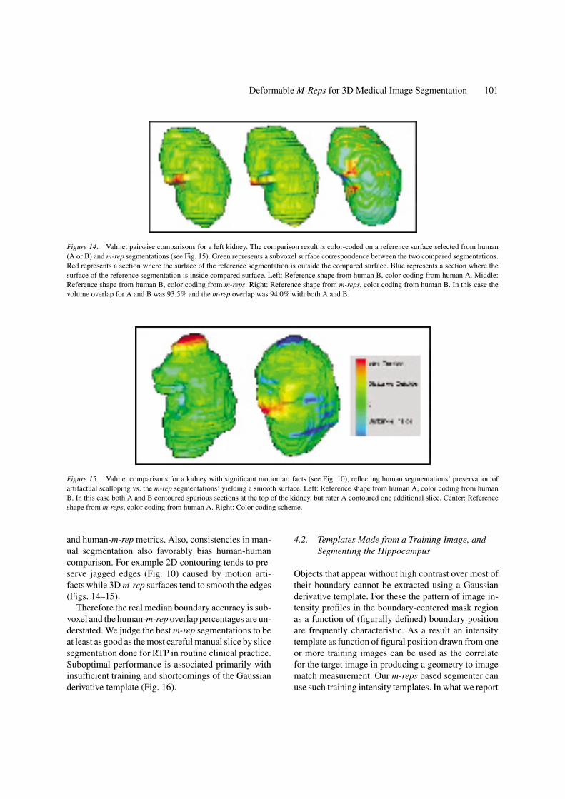
Figure 14. Valmet pairwise comparisons for a left kidney. The comparison result is color-coded on a reference surface selected from human(A or B) and m-rep segmentations (see Fig. 15). Green represents a subvoxel surface correspondence between the two compared segmentations.Red represents a section where the surface of the reference segmentation is outside the compared surface. Blue represents a section where thesurface of the reference segmentation is inside compared surface. Left: Reference shape from human B, color coding from human A. Middle:Reference shape from human B, color coding from m-reps. Right: Reference shape from m-reps, color coding from human B. In this case thevolume overlap for A and B was 93.5% and the m-rep overlap was 94.0% with both A and B.

Figure 15. Valmet comparisons for a kidney with significant motion artifacts (see Fig. 10), reflecting human segmentations’ preservation ofartifactual scalloping vs. the m-rep segmentations’ yielding a smooth surface. Left: Reference shape from human A, color coding from humanB. In this case both A and B contoured spurious sections at the top of the kidney, but rater A contoured one additional slice. Center: Referenceshape from m-reps, color coding from human A. Right: Color coding scheme.

and human-m-rep metrics. Also, consistencies in man-ual segmentation also favorably bias human-humancomparison. For example 2D contouring tends to pre-serve jagged edges (Fig. 10) caused by motion arti-facts while 3D m-rep surfaces tend to smooth the edges(Figs. 14–15).

Therefore the real median boundary accuracy is sub-voxel and the human-m-rep overlap percentages are un-derstated. We judge the best m-rep segmentations to beat least as good as the most careful manual slice by slicesegmentation done for RTP in routine clinical practice.Suboptimal performance is associated primarily withinsufficient training and shortcomings of the Gaussianderivative template (Fig. 16).

4.2. Templates Made from a Training Image, andSegmenting the Hippocampus

Objects that appear without high contrast over most oftheir boundary cannot be extracted using a Gaussianderivative template. For these the pattern of image in-tensity profiles in the boundary-centered mask regionas a function of (figurally defined) boundary positionare frequently characteristic. As a result an intensitytemplate as function of figural position drawn from oneor more training images can be used as the correlatefor the target image in producing a geometry to imagematch measurement. Our m-reps based segmenter canuse such training intensity templates. In what we report

102 Pizer et al.

Figure 16. Correctable m-rep failure mistakenly included in our analysis (worst case in Table 1). Left: Valmet comparison with reference shapefrom human B, color coding from m-reps. Center: Sagittal plane showing m-rep (blue) and human (red) surfaces. Two problems mentionedin the text are illustrated. In the region labeled “A” the m-rep model deformed into structures related to the kidney pelvis that were poorlydifferentiated from the kidney parenchyma. In the region labeled “B” the m-rep model did not elongate fully during the first transformationstage. Right: Transverse plane illustrating the deformation of the m-rep model into peri-pelvic structures in region A. Even in this case there isclose correspondence between human and m-rep contours excluding regions A and B. After more careful user-guided initialization a successfulm-rep segmentation was obtained for this kidney, but those results were omitted in the analysis.

below, we use a template drawn from a single trainingimage with the m-rep fitted by the approach of thispaper into a slightly blurred version of the human’sbinary hand segmentation for that training image.This m-rep fitted into the training segmentation alsoformed the model used in these studies on four othercases.

We first report on using the image intensity profilemethod to fit a hippocampus m-rep from the trainingcase into the slightly blurred versions (Gaussian blur-ring with std. dev. = 1 voxel width) of binary segmen-tations for the four other hippocampi. This processsucceeded in all four cases (Fig. 17), suggesting twoconclusions. First, one can use such fitting of m-repsto already segmented cases to provide statistical de-scription of the geometry via the statistics of the fittedm-reps (Styner, 2002). Second, the method of 3D de-formable m-rep optimization via intensity templates isgeometrically sound.

We move on to the extraction of the left hippocam-pus from MRI, an extraction that is very challengingfor humans and has great variability across human seg-menters. The pattern of intensities across the boundaryof the left hippocampus is characteristic, to the extentthat the structures abutting or near the hippocampusfollow a predictable pattern, with each structure hav-ing its typical intensity in MRI. However, because ofthe variability of this structural pattern and thus thevariability of the intensity pattern, and because of theindistinct contrast at both the tip and the tail of the hip-pocampus, hippocampal segmentation from MRI pro-

vides a major challenge for automatic segmentationof the hippocampus as a single object. The poor con-trast makes it necessary to omit the boundary displace-ment stage from the segmentation and so to stop afterthe medial atom stage. Our method beginning from amanually placed hippocampus model produced a rea-sonable, hippocampus-shaped segmentation overlap-ping with the human segmentation in 3 of the 4 cases(Fig. 17), and in the remaining case, the structural pat-tern around the hippocampus was so different as tomake the method fail. Moreover, in only 1 of the 3semi-successful cases was the segmentation credible toa human rater. However, in each of those 3 cases whenthe same segmentation was begun from the m-rep fit-ted to the human segmentation, it produced a successfulsegmentation with a geometry to image match measurehigher than that achieved when starting from the man-ually placed model. This result suggests that when thecontrast in the images is weak the optimization tech-nique needs to be changed to avoid local optima or thata better measure for geometry-to-image match must befound or that multiple object geometry must be usedin the process. We are investigating all three of thesepaths. In regard to geometry-to-image match, we judgethat the intensity template must really be statistical, re-flecting the range of patterns in a family of trainingimages, and that is indeed a direction that, long since,we have intended our method development to go. Ourfigural coordinate system and correlation method is ex-actly what is needed for such segmentation to be basedon principal components analysis, in a way analagous


Figure 17. Hippocampus results using training intensity matches, for one of the three target images with typical results. The top image showsthe m-rep-segmented hippocampus from the blurred binary segmentation image. Each row in the table shows in three intersecting triorthogonalplanes the target image overlaid with the implied boundary of the m-rep hippocampus segmentation using the image template match. The toprow shows the segmentation from the blurred binary image produced from a human segmentation. The middle row shows the correspondingsegmentation using the mri image as the target and an intialization from a manual placement of the model determined from training image. Thebottom row shows the segmentation of the same target mri with both the initialization and the model being the segmentation result on the blurredbinary image for that case.

to the boundary point based segmentation methods ofCootes and Taylor (1993).

We have found that the figural stage of segmentationusing a training image template is better when the train-ing image intensity template as well as the target imageis rather blurred with a standard deviation of a signifi-cant fraction of the average r of the object. This causessmall differences between the template image and thetarget image in the relative positioning of the objectsought to surrounding structures to have only a smalleffect. Thus when we apply the technique to kidneysegmentation, the fact that, for example, in the trainingimage the kidney nearly abuts the spinal column but is

somewhat separated from it in the target image causesthat portion of the kidney segmented from the targetimage to move toward spine, but only to a small degreeif blurred images are used. With the hippocampus, thissame blurring approach was used, but since the hip-pocampus is much narrower than the kidney, the levelof blurring used was correspondingly smaller.

4.3. Speed of Computation

The speed of a 3D segmentation is 2–4 minutes for a15-atom kidney model on a Pentium 4, 1.8 GHz Dell

104 Pizer et al.

Inspiron 8200 laptop computer, with

• preprocessing computations taking less than1 second,

• the object similarity transform plus elongation stagetaking under 1 second per iteration and on theaverage requiring 8 iterations for a total timeof 2 seconds to determine the object similaritytransform,

• the atom transformations taking on the average ap-proximately 45 seconds per iteration through all ofthe atoms for the kidney, with the time per iterationroughly proportional to the surface area of the object,and the number of iterations required for the kidneybeing 2 to 3, and

• the boundary deformation stage taking approxi-mately 3 seconds.

While the method’s speed has already benefitedstrongly from moving much of the computation fromthe deformation stage to the model building stage, thereis still much room for speedup by more medial levelsof coarse to fine and just by more careful coding.

5. Discussion and Conclusions

The main contribution of this paper is the detailing ofa method for 3D image segmentation that uses the me-dial model representation called m-reps both to captureprior knowledge of object geometry and as the basisof measurement of model to image match. There arenumber of other contributions. We have laid out howto base the geometry in 3D of a figure on a new formof medial atom that allows a spatially sampled rep-resentation while carrying a local ruler and compass.We have described a way of deriving the continuousimplied boundary of a single-figure object from thatrepresentation. We have described a means of calcu-lating a parametrization of space in terms of mediallyrelative positions and signed r -proportional distancefrom this implied boundary and the usefulness of thisparameterization in computing geometric typicality viacorrespondence at the object boundary and computinggeometry to image match via this correspondence andthe correspondence of distances from the boundary inr -proportional terms. This space parametrization alsoallows the interior of the object to be distinguishedas associated with a particular region or in the blendregion. An additional contribution is having a set ofobject and figure based scale levels and the means of

optimal deformation at multiple scale levels by con-sidering the model information at each relevant scale.The initial successes of the segmentation method pro-vide evidence of the usefulness of these ideas. M-repbased visualizations of an object in both 3D and ver-sus the 3D image relative to a medial atom were alsodescribed.

Our quantitative validation on kidney segmentationis encouraging: robust and accurate enough for clini-cal use. A recent study on segmenting the kidney fromCT suggests that the result is very stable to variationsin the manual initialization. However, achieving fullhuman accuracy remains a goal. Controlled, quanti-tated validations on other objects are needed. The re-sults of such a study will be reported in a future paper.We find the results so far, together with the theoret-ical strengths of the deformable m-reps method, en-couraging evidence that this approach will increase themaximum robustness achievable in 3D segmentationof anatomic objects or that it can do such segmentationat a given level of robustness faster than alternativemethods.

At the same time, the method sometimes fails tosegment variants of an object that has significant vari-ability in shape over the population. An example, is theprostate, which varies across individuals in the degreeto which it bends to “saddlebag” around the rectum.In situations of large saddlebagging, the ends of theprostate are so distant from the model that the distance-based geometric penalty prevents convergence to thefully bent prostate at its ends. The solution, we guess,lies in extending the transformation at each scale levelto include not only the transformation listed in Table 1but also a first principal component transformation ofthe collection of medial atoms associated with thatscale level, with the first principal component eigen-mode being computed from a training set.

We have completed the programming for an earlyversion of computing optimal subfigural geometrictransformations, but have not put the program in theform we are ready to test. Each subfigural transforma-tion iteration will require roughly the fraction of thetime for the whole object iteration that the subfigure’sboundary is of the whole object’s boundary. Moreover,the number of iterations can be expected to be distinctlylower than for the whole object, since the intialization,based on the object’s transformation, will typically bebetter than that for the object as a whole. Thus, eachsubfigure transformation will typically take a few tensof seconds.


We have also implemented a means of deformingmultiple objects in a way that the position of oneobject’s implied boundary in another object’s figu-ral coordinates allows rewarding its relationship (e.g.,abutment) to that controlling object (Fletcher, 2002).We need to continue to test this method for the segmen-tation of multiple abutting objects and thus to make thesegmentation method applicable to whole sections ofthe body. With that development our segmentations willform a means of elastic registration between an atlasand a patient’s target image for the whole imaged bodysection. Both the multifigure object segmentation andmultiobject segmentation methods and their validationwill be reported in later papers.

A very pervasive improvement will lie in replacingboth the geometric typicality measures and the geom-etry to image match measures by statistical (log prob-ability) objective functions based on multiple trainingimages. We expect improved performance by the useof a geometric typicality term that is based not sim-ply on distances from a model but instead reflectingnormal variability in a training set, and a geometry toimage match term reflecting image intensity variationsrelative to the geometric model; moreover, that wouldmake it unnecessary to interactively choose a weightfor the geometric typicality term relative to the modelto image match term. The fact that the geometry toimage match module already computes the templatecorrelations that are used in computing the dot prod-uct between an eigenmode and the target image withinthe masked region will make this step straightforward,once the training process is developed. Another direc-tion for future development is the use of mechanical ge-ometric typicality measures in place of statistical oneswhen the transformation is intrapatient rather than be-tween an atlas model and a patient. Here the medialsampling provides promise for strides in efficiency ofmechanical modeling.

Another matter for the future is the evaluation ofthe usefulness of multiple levels of sampling at themedial stages (3 and 4) of the segmentation. Coarsespacing will produce efficient operation but will notaccommodate small radii of curvature relative to theobject width. The accommodation of patches requir-ing these larger curvatures can be done efficiently atthe finer scale medial substages, once the larger scaleoptimization has been accomplished. We will need tostudy when smaller scale wrinkles should be accom-modated at a medial substage and when they can bebetter represented by boundary displacements.

Acknowledgments

We appreciate advice from Valen Johnson and StephenMarron on statistical matters and help from GuidoGerig, Joshua Stough, Martin Styner, and DelphineBull. This work was done under the partial support ofNIH grants P01 CA47982 and EB02779, NSF SGERGrant CCR-9910419, and a fellowship from the LinkFoundation. A gift from Intel Corp. provided comput-ers on which some of this research was carried out.

Notes

1. The reader unfamiliar with the literature on the mathematics ofmedial loci can find the relevant definitions, overview, and refer-ences in Pizer (2003) in this issue.

2. This sheet has both a boundary and singular points in its interior,so in mathematical terminology it is a “stratified set”. We will usethe phrase “medial sheet” to refer to this stratified set.

References

Amenta, N., Bern, M., and Kamvysselis, M. 1998. A new Voronoi-based surface reconstruction algorithm. Computer Graphics Pro-ceedings, Annual Conference Series, 1998, ACM SIGGRAPH:415–422.

Attali, D., Sanniti di Baja, G., and Thiel, E. 1997. Skeleton simplifi-cation through non significant branch removal. Image Processingand Communications, 3(3/4):63–72.

Bittar, E., Tsingos, N., and Gascuel, M. 1995. Automatic recon-struction of unstructured 3D Data: Combining a medial axis andimplicit surfaces. Computer Graphics Forum (Eurographics ’95),14(3):457–468.

Blum, H. 1967. A transformation for extracting new descriptors ofshape. In Models for the Perception of Speech and Visual Form. W.Wathen-Dunn, (Ed.). MIT Press: Cambridge MA, pp. 363–380.

Burbeck, C.A., Pizer, S.M., Morse, B.S., Ariely, D., Zauberman,G., and Rolland, J. 1996. Linking object boundaries at scale: Acommon mechanism for size and shape judgments. University ofNorth Carolina, Computer Science Department, Technical ReportTR94–041. Vision Research., 36(3):361–372.

Catmull, E. and Clark, J. 1978. Recursively generated B-spline sur-faces on arbitrary topological meshes. Computer Aided Design,10:183–188.

Chen, D.T., Pizer, S.M., and Whitted, J.T. 1999. Using multiscalemedial models to guide volume visualization. Tech Report TR99–014, Dept. of Comp. Sci., Univ. of NC at Chapel Hill.

Cootes, T.F., Hill, A., Taylor, C.J., and Haslam, J. 1993. The useof active shape models for locating structures in medical im-ages. In Information Processing in Medical Imaging, H.H. Barrettand A.F. Gmitro (Eds.). Lecture Notes in Computer Science,vol. 687.Springer-Verlag, Heidelberg, pp. 33–47.

Damon, J. 2002. Determining the geometry of boundaries of ob-jects from medial data. Internal report, Dept. of Mathematics,Univ. of NC. Available at webpage http://midag.cs.unc.edu/pubs/papers/Damon SkelStr III.pdf.

106 Pizer et al.

Delingette, H. 1999. General object reconstruction based on sim-plex meshes. International Journal of Computer Vision, 32:111–146.

Fletcher, P.T., Pizer, S.M., Gash, A.G., and Joshi, S. 2002. De-formable m-rep segmentation of object complexes. Proc. Int.Symp. Biomed. Imaging 2002, a compact disc, IEEE. Also avail-able at webpage http://midag.cs.unc.edu.

Fritsch, D.S., Pizer, S.M., Yu, L., Johnson, V., and Chaney, E.L.1997. Localization and Segmentation of Medical Image Objectsusing Deformable Shape Loci. In Information Processing in Med-ical Imaging (IPMI), J. Duncan and G. Gindi (Eds.), LectureNotes in Computer Science, vol. 1230. Springer-Verlag, Heidel-berg, pp. 127–140,

Furst, J.D. 1999. Height Ridges of Oriented Medialness. Ph.D.Thesis, Univ. of NC at Chapel Hill, 1999.

Gerig, G., Jomier, M., and Chakos, M. 2001. Valmet: A new val-idation tool for assessing and improving 3D object segmenta-tion. In Proc. MICCAI 2001, LNCS 2208, Springer, pp. 516–523.

Grenander, U. 1981. Regular Structures: Lectures in Pattern Theory,vol. III, Springer-Verlag, 1981.

Igarashi, T., Matsuoka, S., and Tanaka, H. 1999. Teddy: A sketch-ing interface for 3D freeform design. Computer Graphics Pro-ceedings, Annual Conference Series, 1999, ACM SIGGRAPH,pp. 409–416.

Joshi, S., Pizer, S., Fletcher, P.T., Thall, A., and Tracton, G. 2001.Multi-scale 3-D deformable model segmentation based on me-dial description. Information Processing in Medical Imaging2001 (IPMI ’01). Lecture Notes in Computer Science, vol. 2082,Springer, pp. 64–77.

Kelemen, A., Szekely, G., and Gerig, G. 1999. Three-dimensionalmodel-based segmentation. IEEE-TMI, 18(10):828–839.

Koenderink, J.J. 1990. Solid Shape. MIT Press: Cambridge, MA.Lee, T.S., Mumford, D., and Schiller, P.H. 1995. Neuronal correlates

of boundary and medial axis representations in primate striatecortex. Investigative Ophthalmology and Visual Science AnnualMeeting, abstract #2205.

Leyton, M. 1992. Symmetry, Causality, Mind. MIT Press:Cambridge, MA.

Liu, G.S., Pizer, S.M., Joshi, S., Gash, A.G., Fletcher, P.T., andHan, Q. 2002. Representation and segmentation of multifig-ure objects via m-reps. University of North Carolina ComputerScience Department technical report TR02–037, at webpagehttp://www.cs.unc.edu/Research/MIDAG/pubs/papers/.

Marr, D. and Nishihara, H.K. 1978. Representation and recognitionof the spatial organization of three-dimensional shapes. Proc RoyalSoc, Series B, 200:269–294.

Markosian, L., Cohen, J.M., Crulli, T., and Hughes, J. 1999. Skin:A constructive approach to modeling free-form shapes. ComputerGraphics Proceedings, Annual Conference Series, 1999, ACM,SIGGRAPH, pp. 393–400.

McAuliffe, T., Eberly, D., Fritsch, D.S., Chaney, E.L., and Pizer, S.M.1996. Scale-space boundary evolution initialized by cores. In Vi-sualization in Biomedical Computing (VBC ’96) Proceedings, H.Hoehne and R. Kikinis (Eds.), Lecture Notes in Computer Science,vol. 1131. Springer-Verlag: Heidelberg, pp. 174–182.

McInerny, T. and Terzopoulos, D. 1996. Deformable models in med-ical image analysis: A survey. Medical Image Analysis, 1(2):91–108.

Nackman, L.R. and Pizer, S.M. 1985. Three-dimensional shape de-scription using the symmetric axis transform, I: Theory. IEEETrans. PAMI, 7(2):187–202.

Pizer, S.M., Fritsch, D.S., Yushkevich, P., Johnson, V., and Chaney,E.L. 1999. Segmentation, registration, and measurement of shapevariation via image object shape. IEEE Transactions on MedicalImaging, 18:851–865.

Pizer, S.M., Siddiqi, K., Szekely, G., Damon, J.N., and Zucker, S.W.2003. Multiscale medial loci and their properties. Int. J. Comp.Vis.,55(2/3):155–179.

Pizer, S.M., Fletcher, P.T., Thall, A., Styner, M., Gerig Guido, andJoshi Sarang 2002. Object models in multiscale intrinsic coordi-nates via m-reps. Image and Vision Computing 21:5–15.

Siddiqi, K., Bouix, S., Tannenbaum, A., and Zucker, S. 1999. TheHamilton-Jacobi skeleton. ICCV’99 Proceedings, IEEE, 828–834.

Singh, K. and Fiume, E. 1998. Wires: A geometric deformation tech-nique. In Computer Graphics Proceedings, Annual ConferenceSeries, 1998, ACM SIGGRAPH, pp. 405–414.

Staib, L.H. and Duncan, J.S. 1996. Model-based deformable surfacefinding for medical images. IEEE Trans. Med. Imaging, 15(5):1–12.

Styner, M. and Gerig, G. 2001. Medial models incorporating objectvariability for 3D shape analysis. Information Processing in Medi-cal Imaging 2001 (IPMI ’01). Lecture Notes in Computer Science,Springer, 2082:502–516.

Styner, M., Gerig, G., Lieberman, J., Jones, D., and Weinberger,D. 2002. Statistical shape analysis of neuroanatomical structuresbased on medial models Medical Image Analysis, to appear.

Thall, A. 2003. Deformable solid modeling via medial sam-pling and displacement subdivision. UNC Computer ScienceDept., Dissertation to be defended August 2003, at webpagehttp://www.cs.unc.edu/Research/MIDAG/pubs/phd-thesis.

Tracton, G., Chaney, E.L., Rosenman, J.G., and Pizer, S.M. 1994.MASK: Combining 2D and 3D Segmentation methods to enhancefunctionality. Math. Methods Med. Imaging III, F.L. Booksteinet al. (Eds.), SPIE Proc. 2299:98–109.

Vermeer, P.J. 1994. Medial axis transform to boundary representationconversion, Ph.D. Thesis, Purdue University, May 1994.

Yushkevich, P., Pizer, S.M., and Culver, T. 1999. Statistical objectshape via a medial representation. Tech Report TR00–002, Dept.of Comp. Sci., Univ. of NC at Chapel Hill.

Wyvill, G., McPheeters, C., and Wyvill, B. 1986. Data Structures forsoft objects. Visual Computer, 2(4):227–234.

Deformable M-Reps for 3D Medical Image...

Documents

Transcript of Deformable M-Reps for 3D Medical Image...