306-1

Defining Geological Units by Grade Domaining

Xavier Emery1 and Julián M. Ortiz1

1Department of Mining Engineering, University of Chile

Abstract

Common practice in mineral resource estimation consists in partitioning the ore body into several domains defined by grade intervals, prior to the geostatistical modeling and estimation at unsampled locations. This paper shows the pitfalls of grade domaining through a case study in which we compare the performance of several estimation schemes and demonstrate that the use of domains defined by grade cutoffs implies a deterioration of the resource estimates, mainly in what refers to accuracy and conditional bias. Then, several conceptual limitations of the grade domaining approach are stressed, in particular the fact that it does not account for the spatial dependency between adjacent domains and for the uncertainty in the domain boundaries. Also, this approach is shown to be sensitive to the cutoffs that define the domains, to provoke artifacts in the kriged maps, histograms and scattergrams between true and estimated grades, and to lower the kriging variance, a feature that may impact the mineral resource classification. An alternative approach is proposed to overcome these limitations, based on a stochastic modeling of the grade domains and a cokriging of the grades from all the domains.

Introduction

Geological modeling is a key step prior to geostatistical estimation or simulation of the grades within a mineral deposit. Although alteration, mineralization and lithological aspects should be considered in determining the geological model (domaining) for interpolation, common practice consists in contouring the grades, generating grade shells (Duke and Hanna, 2001). Within each shell the grades are considered homogeneous and can therefore be interpreted as a realization of a stationary random function, allowing variogram modeling and subsequent kriging or conditional simulation. Such grade domaining or grade zoning is often done in association with mineralogical classification, for instance for each mineralogical unit, a high-grade, medium-grade and low-grade domains are defined and analyzed separately, in an attempt to better forecast the performance of the processed ore in the mill. Although the definition of geological domains by grade contouring is a common approach in the mineral industry, very few references to this subject can be found in the literature (Stegman, 2001; Guibal, 2001).

In this article, we discuss some of the problems of using grade shells from a practical and theoretical viewpoint and we propose a better way to use them in resource estimation.

The work has been divided in three sections. First, we show the consequences of using grade shells for the definition of geological domains and the resource estimation by an application to a porphyry copper deposit. The ideal case of perfectly known boundaries between grade domains, and the case of estimated boundaries are compared through a jackknife with the true values obtained from production blast holes. This empirical study shows the impoverishment of the results as errors are added through the estimation of the shell boundaries, which is always the case in practice. Second, we present a general discussion of the grade domaining approach from a theoretical standpoint. The arbitrary definition of the cutoffs to define the grade domains and the problems arisen from the uncertainty in their boundaries are pointed out, with emphasis on the artifacts this approach generates in the resulting estimated or simulated grades. In the last section, we propose a solution to avoid some of these limitations, which consists in weighting the grade estimates obtained for each domain by the probability of occurrence of such domain.

306-2

An Empirical Case Study

Presentation of the Data and Methodology

The case study concerns a Chilean porphyry copper deposit for which two datasets are available: a set of over two thousand samples from a diamond-drill hole exploration campaign, and a set of more than twenty thousand blast hole samples that cover approximately the same area than the exploration drill holes (Fig. 1a and 1b). All the data (from drill holes and blast holes) represent twelve-meter long composites in which the copper grade has been sampled and assayed. The grade histogram is close to a lognormal distribution (Fig. 1c) with a mean close to 1.0% Cu, whereas the variogram shows an anisotropy with a greater continuity along the vertical direction than in the horizontal plane (Fig. 1d). The data belong to a unique geological population (in terms of alteration, mineralization and lithology) and it is used to illustrate the consequences of domaining based on grade cutoffs.

The study consists in using the information from the drill hole dataset to estimate the blast hole grades, a procedure known in geostatistics as “jackknife” (Efron, 1982). Several estimations are performed in order to assess the effect of using grade-based domains:

1. Case 1: traditional resource estimation is performed via ordinary kriging without grade domaining. This first case will constitute a reference for comparisons; it will also be used for estimating the grade shell boundaries for the other cases.

2. Grade domaining is applied previous to estimation by ordinary kriging. Three cases are considered:

a. Case 2: three grade domains are defined for resource estimation: a low-grade domain (copper grade between 0% and 0.5%), a medium-grade domain (from 0.5% to 1.0%) and a high-grade domain (above 1.0%).

b. Case 3: again three grade domains are used, but the cutoffs are changed to assess the impact of the choice of the cutoffs. The new geological domains are now defined by cutoffs 0.7% and 1.5%. This case allows assessing the impact of the election of the cutoffs.

c. Case 4: four cutoffs are used to define five grade domains: 0.5%, 0.7%, 1.0% and 1.5%. This case allows assessing the impact of increasing the number of grade shells used to perform resource estimation.

Note that every kriging requires performing a variogram analysis per grade domain. For each case, two sub-cases are distinguished:

a) Ideal situation, for which the blast holes are classified in the grade domain corresponding to their true grades (no misclassification), and

b) Effective situation, for which the classification is based on the estimated grades obtained in the reference case, so that some blast holes may be misclassified.

This second situation is realistic whereas the first one constitutes only a basis for comparison, since it can never be achieved in practice: the grade zoning is always defined according to an interpretation of the deposit from exploration information.

It should be noticed that, in practice, geological domains are defined by hand contouring from a geological interpretation of the deposit. Grade shells are drawn using the intersects of drill hole data, considering the cutoffs defined for defining the domains. The use of ordinary kriging for this case study constitutes another way to create the grade shells. This is a repeatable approach and it considers the spatial continuity of the grades in all directions.

306-3

Figure 1. Location maps of a, drill hole and b, blast hole data (representation of one bench); c, histogram and d, variogram for the copper grades

Accuracy of Grade Estimations

The results obtained for each situation are summarized in Table 1, through basic statistics on the estimation errors at the blast hole locations. The reference case (case 1) corresponds to ordinary kriging without domaining. Cases identified with the letter a assume each location is assigned exactly to its true grade domain, while cases noted with b correspond to the situation where the grade domain assigned to a location is inferred from the surrounding information.

case 1 case 2a case 3a case 4a case 2b case 3b case 4b

mean error (% Cu) 0.009 0.017 0.028 0.020 -0.022 -0.017 -0.026

mean absolute error

(% Cu) 0.387 0.265 0.232 0.184 0.432 0.435 0.431

root of the mean squared error

(% Cu) 0.623 0.511 0.450 0.430 0.690 0.721 0.715

Table 1. Statistics on the estimation errors at the blast hole locations

306-4

In every case, the grade estimation is unbiased since the average error is close to zero: the unbiasness is actually a general property of ordinary kriging and should be always fulfilled, unless strong mistakes are made in the definition of the grade domains (for instance, if the spatial extension of the high-grade domain is overstated). Henceforth, we focus on the two other criteria (mean absolute and root of the mean squared errors), which measure the average amplitude of the error and therefore indicate the accuracy of the estimation.

In this respect, the ideal cases, for which the delineation of the grade shells is error-free, always improve the results of the reference case. This observation proves that the knowledge of the true grade contours is a valuable information for mineral resource estimation. This can be illustrated by considering the scattergram between true and estimated grades (Fig. 2a and 2b): when grade domaining is used, the cloud of points is constrained to the sectors along the first bisector that are delimitated by the cutoffs used for domaining, hence a lower dispersion around the first bisector is achieved. Furthermore, if this ideal case could be achieved, the estimation would necessarily improve as more domains were added, and in the extreme case where a series of very tight grade intervals are used, estimation could be solely based on the grade domaining.

However, the effective cases, for which the grade shell delineation is only estimated, lead to poorer results than the reference situation. The explanation comes from the blast hole misclassifications when performing the estimation within each grade domain. Indeed, although a blast hole is classified as low-graded, in reality it can belong to another grade domain, hence the scattergram between true and estimated grades presents “stripes” and has a greater dispersion around the first bisector (Fig. 2c). From now on, only the effective cases will be discussed, since the ideal case is unrealistic: a perfect definition of the grade domains is never met in practice

Figure 2. Scattergrams between true and estimated grades for the reference, an ideal and an effective case

306-5

Conditional bias

An important feature of the scattergrams between true and estimated grades displayed in Figure 2 is to determine whether conditional bias exists, that I, the expected value of the true grade given the estimated grade at the same location is not equal to the true grade (Journel and Huijbregts, 1978, p. 458). Such property has a great impact on the assessment of recoverable reserves. Indeed, at the time of exploitation, the selective mining units are sent to mill or dump depending on whether their estimated grade (not their true grade which is unknown) is above or below a given cutoff. In case of conditional bias, the average estimated grade of the mining units sent to mill does not match their true average grade.

In the example, the estimations performed without grade zoning (case 1) are almost conditionally unbiased. Instead, a conditional bias appears when resorting to a grade domaining, as shown in Table 2. This can be explained by considering that once the high and intermediate-grade domains are defined, they are filled with high or intermediate estimated grades, but in reality they may contain sectors with lower grades, hence an overestimation is made. This always occurs if a non-zero cutoff is applied (bold figures in Table 2).

cutoff (% Cu) 0.0 0.5 1.0 1.5

true 1.17 1.22 1.47 1.90 case 1 estimated 1.16 1.22 1.51 2.08 true 1.17 1.22 1.47 1.72 case 2b estimated 1.19 1.29 1.67 1.99 true 1.17 1.26 1.43 1.90 case 3b estimated 1.19 1.32 1.49 2.33 true 1.17 1.22 1.47 1.90 case 4b estimated 1.20 1.27 1.61 2.33

Table 2. Statistics for conditional bias (mean grade above a cutoff)

In the next section, we discuss some other pitfalls of the grade zoning approach from a theoretical point of view. The case study is also used to illustrate some of these conceptual problems.

Other Conceptual Limitations of Grade Domaining

Dependency Between Grade Domains

A first theoretical limitation of the grade zoning approach stems from the dependency between the different domains caused by the spatial continuity of the grades in the deposit. In general, boundaries defined by grade domaining are not hard, that is, there is spatial correlation between the grades at both sides of the boundary. However, the estimation within a domain usually omits information of the adjacent domains, hence it loses accuracy, especially in the boundaries of the domain. Estimating the grades in each domain separately means that these domains are considered as independent: this creates a boundary that does not exist geologically and contradicts the assumption of spatial continuity (correlation) in the grade distribution.

The spatial dependency between domains (defined by grade shells or by mineralogical considerations) could always be taken into account in the mineral resource estimation, for example through a cokriging approach.

306-6

Uncertainty in the Domain Boundaries

In practice, grade shells are determined by hand contouring intersects of the drill holes with low, medium, and high grade zones in cross sections. Then wireframing is used to define the volumes (grade shells), with the consequent possibility of inconsistent volumes – grade shells may cross each other – and the little repeatability of the process. Another approach to define the domains is to use a quick interpolation of the available samples (in general, drill hole cores) and then define the domains from its result. In any case, the domain boundaries may not be accurate.

Now, in general, the grade zoning approach does not allow accounting for the uncertainty in the shell boundaries and for possible misclassifications of the unsampled locations. This can have far-reaching consequences in the estimated ore tonnages and, therefore, in the economic appraisal of the mining project. For instance, let us consider a domain defined by the grade interval [a,b]. The estimations at the unsampled locations in this domain usually lie in [a,b] since they only use data that belong to such interval. As a consequence, the tonnage of material whose grade belongs to [a,b] practically does not depend on the variogram or the kriging parameters defined by the user. If the grade domains are numerous, the same reasoning proves that the whole grade-tonnage curve is pre-determined by the partitioning into grade shells, before performing the geostatistical modeling and kriging. This approach is clearly not advisable for ore reserve estimation, unless the deposit is so well understood that the grade domaining is unquestionable. For instance in case the spatial extension of the high-grade domain is overestimated (e.g. waste wrongly classified as ore), the total amount of recoverable reserves is likely to be overstated.

In conclusion, the delineation of the grade domains must be performed with extreme care. In general, the true contours are much more irregular than the interpreted contours, since the interpolation of the unsampled grades (by kriging or inverse distance weighting) on which the interpretation is based is always smoother than the reality (Fig. 3) (Journel and Huijbregts, 1978, p. 553). We strongly recommend the user to perform a sensitivity study and compare several domaining schemes in order to assess the potential impact of the uncertainty in the spatial extensions of the different domains.

Figure 3. Comparison of the true and estimated contour shells associated with cutoffs 0.5%, 0.7%, 1.0% and 1.5% (representation of one bench)

306-7

Artifacts in Maps, Histograms and Scattergrams

To illustrate the artifacts generated by using grade domains, consider the previous application, in which a domain is defined by a grade interval [a,b]. Because of the smoothing effect of kriging, the estimated grade will approximate the average grade in this domain, say (a+b)/2. Hence, a concentration of grades near this average value is observed, with a resulting decrease in the amount of grades near both cutoffs a and b. This can be seen as steps on a cumulative histogram. As a consequence, the map of the estimated grades will present abrupt transitions when crossing the boundary between two grade domains, their histogram will be multimodal (Fig. 4), whereas the scattergram between true and estimated values will show “stripes”, as presented in Figure 2c. Such artifacts will be more pronounced when more cutoffs (more domains, like in case 4) are used in the partitioning of the deposit and may be dangerous for the valorization of the ore body, particularly if one of these cutoffs has an economic signification, e.g. for distinguishing ore and waste.

When simulation is used, discontinuity will exist at the boundary between two grade domains, since only the information belonging to the geological unit of the simulated location is considered and all other information (from different grade intervals) is disregarded. The post-processing of these simulated models will again reflect the effect of this modeling approach. This could be partially solved by integrating the information from all the grade shells via a multivariate approach (cokriging).

Figure 4. An example of map and histogram for the estimated grades

Sensitivity to the Cutoff Definition

The definition of the grade domains is sometimes made on the basis of the grade histogram, via the analysis of statistical tools such as log-probability plots. Some practitioners interpret a change of slope in the log-probability plot as a mixture of populations and, from this interpretation, define a set of cutoffs that are deemed relevant for grade zoning. This approach is questionable since, in general, a nonlinear log-probability plot indicates a departure from lognormality rather than the presence of several populations (Sinclair and Blackwell, 2002, p. 92), hence the grade domains have no physical meaning. Furthermore, the number and values of the cutoffs used to define the grade domains have an important impact on the estimation results. For instance, in the previous case study, the estimations obtained in case 1b are poorly related with the ones obtained in case 2b (Fig. 5), although the kriging neighborhood is unchanged and the variograms are not so different between both cases. This high sensitivity to the definition of the domains proves that such approach is unreliable and should be avoided.

306-8

Self-justificatory Approach

The partitioning of a deposit in several geological domains is often validated by comparing the statistical characteristics of the grades in the different domains, in particular their histogram and variogram. Now, in case of using grade shells, such statistical validation is often misleading. Concerning the histogram, by definition of the grade zoning approach, a hierarchy will be observed between the different domains, for instance in what refers to their mean grade. The following result might be less obvious to the practitioner: strong differences are also expected when comparing the grade variograms in different domains. Indeed, in many deposits (copper, uranium, precious metals, etc.), the spatial distribution of grades is ruled by a property known as “destructuring of extreme values” (Matheron, 1982; Goovaerts, 1997, p. 278), which states that the extreme values do not cluster in space, i.e. the occurrence of extreme values is purely random. In mathematical terms, the destructuring of extreme values means that the simple and cross covariances of indicator variables get close to a pure nugget effect when the indicator thresholds are very low or very high. Consequently, the extreme-grade domains are expected to have a covariance with a higher relative nugget effect than the intermediate-grade domains. An illustration of this statement is given in Figure 6.

In summary, although the spatial distribution of the grades in the deposit is homogeneous, the comparison of the histograms and variograms between grade domains will always lead to the conclusion that these domains have very different statistical behavior, hence that grade zoning is justified. Geological knowledge should always mandate whether different geological domains can be considered or not. This decision should not be based solely on statistical analyses.

Figure 5. Comparison of the estimations obtained by varying the grade domain definition

306-9

Figure 6. Standardized variograms for two grade domains: 0.5%-1.0% (continuous line) and > 1.0% (dashed line)

Bias in the Kriging Variance

A last drawback of the partitioning by grade cutoffs concerns the kriging variance. In each domain, the grades are restrained to a limiting interval, hence their dispersion is lower than the one of the global histogram and is closely related to the definition of the cutoffs used for grade zoning. This also occurs with the variogram sill of the grades within each domain, and consequently the kriging variance, which strongly depends on the variogram model. The underestimation of the kriging variance may lead to the wrong idea that the unsampled grades are well estimated. The problem comes from not incorporating in the estimation variance the uncertainty on the grade shells.

The kriging variance is sometimes used as a ranking index for classifying the estimated grades by increasing order of uncertainty, for instance to classify the mineral resources into measured, indicated or inferred categories (Royle, 1977; Sabourin, 1984; Froidevaux et al, 1986; Blackwell, 1998). In consequence, the classification becomes an artifact of the grade zoning imposed: for instance, if the high grade areas are partitioned into many domains corresponding to small grade intervals, these areas are likely to be classified as measured resources, even if they are under-sampled.

A Proposal

Methodology

In this section, we propose an approach to estimate the mineral resources using grade shells. For clarity, the proposal is presented using the case study, for which three grade domains are defined: below 0.5%, from 0.5% to 1.0% and above 1.0%. This is referred to as “case 5”. Henceforth, the grade at location x will be denoted as Z(x) (in the geostatistical formalism, this is a random variable).

The proposed methodology consists of the following steps:

a) Estimate the probabilities for the unsampled locations to belong to each grade domain, i.e.

306-10

≤=<≤=<≤=

])(Z%0.1[Prob)(P%]0.1)(Z0.5%[Prob)(P

0.5%])(Z0.0%[Prob)(P

3

2

1

xxxxxx

An indicator kriging or cokriging approach can be used (Goovaerts, 1997, p. 337); a post-processing step is then necessary to ensure the consistency of the estimated probabilities, i.e. make sure that P1(x), P2(x) and P3(x) are nonnegative and sum to one at any location x (Goovaerts, 1997, p. 338). Alternatively, one may resort to conditional simulation of random sets to draw realizations of the grade domains and derive the previous probabilities; this option is more demanding since it requires a spatial distribution model for the random sets, for instance a truncated Gaussian or a plurigaussian model (Armstrong et al., 2003).

b) Consider the grade in each domain as a particular regionalized variable, which defines three different random fields:

≤=<≤=<≤=

])(Z%0.1|)(Z[)(Z%]0.1)(Z0.5%|)(Z[)(Z

0.5%])(Z0.0%|)(Z[)(Z

3

2

1

xxxxxxxxx

c) Perform a variogram analysis of the coregionalization {Z1, Z2, Z3}. Since these random fields are defined on non-overlapping domains (case of total heterotopy), the assessment of the cross-structures is not easy. One may use the cross-covariance as a structural tool (Larrondo, Leuangthong and Deutsch, 2004). The nugget effects of the cross-structures remain unknown, however they are not required in the cokriging system (following step) (Wackernagel, 2003, p. 158).

d) Perform a cokriging of the coregionalization. At each blast hole location, one obtains a set of estimates (one per grade domain), say Z1

*, Z2* and Z3

*.

e) The final grade estimation is obtained by weighting the previous estimates by the probability of belonging to the corresponding domain:

)(Z)(P)(Z)(P)(Z)(P)(Z *33

*22

*11

* xxxxxxx ++=

Application and Discussion

The previous methodology is applied to the copper case study, by using an ordinary indicator cokriging for step a) and an ordinary cokriging for step d). Figure 7 displays the scattergram between true and estimated grades at the blast hole locations, which is quite similar to the one obtained in the reference case (Fig. 2a). The statistics for measuring the accuracy and conditional bias are summarized in Tables 3 and 4 and are quite satisfactory (the mean absolute and quadratic errors are even less than in the reference case).

306-11

Figure 7. Scattergrams between true and estimated grades

mean error (% Cu)

mean absolute error (% Cu)

root of the mean squared error (% Cu)

case 5 0.044 0.374 0.602

Table 3. Statistics on the estimation errors at the blast hole locations

cutoff (% Cu) 0.0 0.5 1.0 1.5

true 1.17 1.21 1.48 1.97 case 5 estimated 1.13 1.17 1.43 1.96

Table 4. Statistics for conditional bias (mean grade above a cutoff)

The proposed approach has its pros and cons. On the one hand, the uncertainty in the domain boundaries and the dependency between grade domains are taken into account, via a probabilistic modeling of the domains (step a) and a cokriging of the grades (step d) respectively. Furthermore, one has a data-charged model for describing the spatial distribution of grades, by using a different variogram for each grade domain; this allows incorporating structural changes in the grade distribution, e.g. a change in the anisotropy orientation when the grade increases.

On the other hand, the approach has several drawbacks:

• First, it requires much more work than a classical kriging, especially in what refers to variogram analysis, hence it is not suitable when many grade domains are defined. In such case, there may even be too few data per domain to perform the variogram inference.

• Second, the user must pay attention to the neighborhood search radii in order to find enough data for cokriging (step d); for instance, the high-grade area contains few Z1-data, which makes difficult estimation of Z1

*.

• Third, the method implicitly assumes that there exists a hard boundary between the grade domains: indeed ordinary cokriging supposes that the mean grades are unknown but differ from one domain to another, hence the transition is not continuous.

306-12

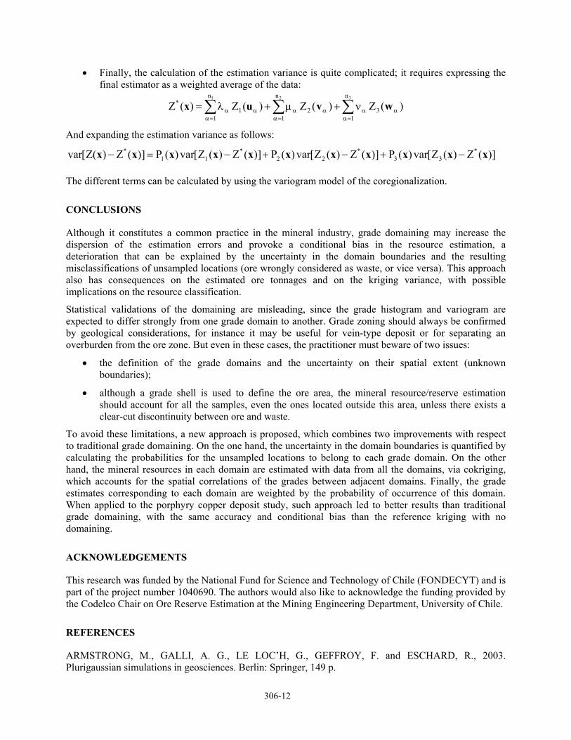
• Finally, the calculation of the estimation variance is quite complicated; it requires expressing the final estimator as a weighted average of the data:

∑∑∑=α

αα=α

αα=α

αα ν+µ+λ=321 n

13

n

12

n

11

* )(Z)(Z)(Z)(Z wvux

And expanding the estimation variance as follows:

])(Z)(Z[var)(P])(Z)(Z[var)(P])(Z)(Z[var)(P])(Z)(Z[var *33

*22

*11

* xxxxxxxxxxx −+−+−=−

The different terms can be calculated by using the variogram model of the coregionalization.

CONCLUSIONS

Although it constitutes a common practice in the mineral industry, grade domaining may increase the dispersion of the estimation errors and provoke a conditional bias in the resource estimation, a deterioration that can be explained by the uncertainty in the domain boundaries and the resulting misclassifications of unsampled locations (ore wrongly considered as waste, or vice versa). This approach also has consequences on the estimated ore tonnages and on the kriging variance, with possible implications on the resource classification.

Statistical validations of the domaining are misleading, since the grade histogram and variogram are expected to differ strongly from one grade domain to another. Grade zoning should always be confirmed by geological considerations, for instance it may be useful for vein-type deposit or for separating an overburden from the ore zone. But even in these cases, the practitioner must beware of two issues:

• the definition of the grade domains and the uncertainty on their spatial extent (unknown boundaries);

• although a grade shell is used to define the ore area, the mineral resource/reserve estimation should account for all the samples, even the ones located outside this area, unless there exists a clear-cut discontinuity between ore and waste.

To avoid these limitations, a new approach is proposed, which combines two improvements with respect to traditional grade domaining. On the one hand, the uncertainty in the domain boundaries is quantified by calculating the probabilities for the unsampled locations to belong to each grade domain. On the other hand, the mineral resources in each domain are estimated with data from all the domains, via cokriging, which accounts for the spatial correlations of the grades between adjacent domains. Finally, the grade estimates corresponding to each domain are weighted by the probability of occurrence of this domain. When applied to the porphyry copper deposit study, such approach led to better results than traditional grade domaining, with the same accuracy and conditional bias than the reference kriging with no domaining.

ACKNOWLEDGEMENTS

This research was funded by the National Fund for Science and Technology of Chile (FONDECYT) and is part of the project number 1040690. The authors would also like to acknowledge the funding provided by the Codelco Chair on Ore Reserve Estimation at the Mining Engineering Department, University of Chile.

REFERENCES

ARMSTRONG, M., GALLI, A. G., LE LOC’H, G., GEFFROY, F. and ESCHARD, R., 2003. Plurigaussian simulations in geosciences. Berlin: Springer, 149 p.

306-13

BLACKWELL, G. H., 1998. Relative kriging errors – a basis for mineral resource classification. Exploration and Mining Geology, Vol. 7, No. 1-2, p. 99-106.

CHILÈS, J. P. and DELFINER, P., 1999. Geostatistics: Modeling spatial uncertainty. New York: Wiley, 696 p.

DUKE, J. H. and HANNA, P. J., 2001. Geological Interpretation for Resource Modelling and Estimation, in Mineral Resource and Ore Reserve Estimation – The AusIMM Guide to Good Practice, A. C. Edwards, editor, pp. 147-156. The Australasian Institute of Mining and Metallurgy, Melbourne, Australia.

EFRON, B., 1982. The jackknife, the bootstrap, and other resampling plans. Society for Industrial and Applied Mathematics, Philadelphia.

FROIDEVAUX, R., ROSCOE, W. E. and VALIANT, R. I., 1986. Estimating and classifying gold reserves at Page-Williams C zone: a case study in nonparametric geostatistics. In: Ore reserve estimation: methods, models and reality, Montreal: Canadian Institute of Mining and Metallurgy, p. 280-300.

GOOVAERTS, P., 1997. Geostatistics for natural resources evaluation. New York: Oxford University Press, 480 p.

GUIBAL, D., 2001. Variography, a Tool for the Resource Geologist, in Mineral Resource and Ore Reserve Estimation – The AusIMM Guide to Good Practice, A. C. Edwards, editor, pp. 221-236. The Australasian Institute of Mining and Metallurgy, Melbourne, Australia.

JOURNEL, A. G. and HUIJBREGTS, C. J, 1978. Mining Geostatistics. London: Academic Press, 600 p.

LARRONDO, P., LEUANGTHONG, O. and DEUTSCH, C. V., 2004, Grade estimation in multiple rock types using a linear model of coregionalization for soft boundaries, In: International Conference Mining Innovation Minin 2004, Magri, E., et al. (eds.), in press.

MATHERON, G., 1982. La déstructuration des hautes teneurs et le krigeage des indicatrices. Internal report N-761, Centre de Géostatistique, Ecole Nationale Supérieure des Mines de Paris, Fontainebleau, 33 p.

ROYLE, A. G., 1977. How to use geostatistics for ore reserve classification. Eng. Min. Journal, February, p. 52-55.

SABOURIN, R., 1984. Application of a geostatistical method to quantitatively define various categories of resources. In: Geostatistics for Natural Resource Characterization, Verly, G., M. David, A. G. Journel, and A. Maréchal (eds.), Dordrecht: Reidel, vol. 1, p. 201-215.

SINCLAIR, A. J., and BLACKWELL, G. H., 2002. Applied mineral inventory estimation. Cambridge: Cambridge University Press, 381 p.

STEGMAN, C. L., 2001. How Domain Envelopes Impact on the Resource Estimate – Case Studies from the Cobar Gold Field, NSW, Australia, in Mineral Resource and Ore Reserve Estimation – The AusIMM Guide to Good Practice, A. C. Edwards, editor, pp. 221-236. The Australasian Institute of Mining and Metallurgy, Melbourne, Australia.

WACKERNAGEL, H., 2003. Multivariate geostatistics: an introduction with applications. Berlin: Springer, 387 p.