Defining apartment neighbourhoods with Thiessen polygons and fuzzy equality clustering

Paper submitted for presentation at the

18th Annual Conference of the European Real Estate Society,

Eindhoven, the Netherlands, 15-18 June 2011

Marko Kryvobokov PhD, researcher

Laboratory of Transport Economics (LET), Lyon, France

Address: LET-ISH, 14 Avenue Berthelot, F-69363, Lyon Cedex 07, France

E-mail: mark.kryvobokov@let.ish-lyon.cnrs.fr

Abstract Purpose – The purpose of the paper is to verify whether the version of neighbourhoods created from the lowest geographical level improve a predictive accuracy of hedonic model in comparison with those based on upper geographical levels. Methodology/approach – The paper proposes a method for defining neighbourhoods from Thiessen polygons created around the points of apartments. These polygons occupy the whole analysed area and are used as the spatial units for clustering. The clustering technique is based on contiguity of polygons and fuzzy equality of the principal components of their attributes. Clustering is started at different geographical levels: municipalities, smaller traffic analysis zones, and apartments’ Thiessen polygons. The ordinary least squares (OLS) and spatial error techniques are applied in hedonic price models with different versions of neighbourhoods. Originality/value – Neighbourhoods can be defined using the Thiessen polygons of individual observations. This very “bottom up” approach can minimise dependency from existing political, administrative and other boundaries. The clustering technique is based on fuzzy equality and does not need the a priori determination of a number of clusters, while contiguity and hierarchical nature of neighbourhoods are considered. Findings – With OLS regression, the superiority of Thiessen polygons is evident in both in-sample analysis and ex-sample prediction. When we control for spatial effect with a spatial error technique, the clusters of Thiessen polygons do not always provide the best outcome, and their superiority is contested by the highest geographical level of municipalities. Keywords: apartment, neighbourhood, Thiessen polygon, clustering, hedonic model. Paper type: research paper

1. Introduction Since the appearance of the seminal paper of Rosen (1974)1, a hedonic price model is widely exploited by public administration, business and academia to estimate the willingness to pay for different attributes. In the real estate domain, the popularity of this methodology used for mass valuation can be explained by its applicability in urban planning, property tax assessment, mortgage loan support and price indices calculation to name just several applications. In a hedonic price model, the dependent variable is usually a sale price of real estate and the explanatory variables are sale date, structure description and location data. In this study we place emphasis on location. Heterogeneity of space and complexity of its perception exemplify the fact that the analyses of “location, location, location” in the hedonic context are very rich and many-sided. The influence of different positive and negative externalities on property value can be measured with distance or travel time variables. However, Ross et al. (2009) have highlighted the common inability to fit more than two distance variables in hedonic model arguing that two points in space triangulate the optimal position by fundamental geometry. This study addresses the issue of location in a hedonic price model focusing on the detection of neighbourhoods, within which identical properties can be seen as reasonably close substitutes. Differently from the concept of geographical submarkets, where separate hedonic models are calibrated, neighbourhoods are included in an overall regression model either as binary (dummy) variables or as the variables of interaction of neighbourhood dummies with some neighbourhood attributes, as e.g. average living area and age in Fletcher et al. (2000). There are, among others, two kinds of problems with submarkets and neighbourhoods identification. First, formal clustering methods are not always applied, and even if they are used, they need a number of clusters to be specified a priori, which leads to multiple experiments to find an optimal number. Second, very few studies start at the lowest possible geographical level, i.e. at the level of individual properties; more often such existing territorial units as administrative districts or census tracks are used as a geographical base. To increase the degree of objectivity in a neighbourhood delineation process and its independence from existing territorial units, in this study we propose a formal clustering method based on fuzzy equality and started at the level of individual observations. We admit however that it is hardly possible to be completely independent from the existing fixed boundaries, first and foremost because statistical data are collected within them.

1 Though there were several predecessors, e.g. Pendleton (1965), the impact of their works was not as resounded as of the theoretically solid paper of Rosen, which is a standard reference in the hedonic price literature.

In the proposed method, Thiessen polygons are created around the points of observations. This transformation from points to polygons has two advantages: it allows, first, occupying the whole analysed territory, and second, applying the concept of contiguity. When a sample is divided into one part for estimation (the in-sample) and the other part for prediction evaluation (the ex-sample), the former issue is important, because all the ex-sample points can geographically belong to clusters already established by the in-sample observations. The later issue can be exploited for pure geographical clustering taking into account polygonal boundaries. The clustering technique is based on fuzzy equality of polygon attributes and contiguity of polygons. The procedure itself determines a number of clusters. The hierarchical nature of neighbourhoods is mirrored in the iterative process of clustering. In hedonic regression modelling, ordinary least squares (OLS) and spatial error methodologies are applied with an in-sample analysis and ex-sample prediction. While model performance is important for understanding the impact of different attributes on sale price, in the academic literature the emphasis has been shifted to out-of-sampling predictive accuracy (e.g. Bourassa et al., 2003; Case et al., 2004; Wilhelmsson, 2004), which is particularly important in tax assessment and other cases when good prediction is necessary. The purpose of the paper is to verify whether the version of neighbourhoods based on the lowest geographical level improve a predictive accuracy of hedonic model in comparison with those based on upper geographical levels. Thus, bigger territorial units of municipalities and traffic analysis zones are exploited as base spatial units for clustering to detect the alternative versions of neighbourhoods. We admit that the analysed area, which is the adjacent cities of Lyon and Villeurbanne, is large enough to be an object of market segmentation. Nevertheless, in this study, we limit ourselves by the delineation of neighbourhoods and do not deal with submarkets. It is related to the peculiarities of the proposed method, which is often unable to unite more than a few observations. Moreover, in contrast to most of studies of market segmentation and neighbourhoods exploring individual housing markets, we analyse apartment market. Apartments in the same apartment block can be very different not only by their surface or number of rooms, but also by the level of street noise around the different sides of a block, apartment state due to individual approaches to maintenance, etc. The rest of the paper is organised as follows. The next section is literature review, mainly focused on geographical market segmentation and neighbourhood delineation. The third section describes in detail the proposed clustering method. The fourth section is about the study area and data used. Sections five and six are devoted to the application of the proposed method: clustering of Thiessen polygons and other territorial units, and incorporation of neighbourhoods in hedonic models respectively. The final section concludes.

2. Literature review A comprehensive overview of the literature on location influence patterns in mass valuation can be found in the doctoral dissertation of Borst (2007). According to him, the most straightforward approach is to divide the universe of properties into subgroups for which the effects of location is similar. The two widely applied techniques are market segmentation and neighbourhood delineation. Because a sort of confusion exists in the literature in respect to the notions of submarkets and neighbourhoods, it is important to note that in this study we use the following definitions. In each geographical segment (submarket) detected with spatially-based or characteristics-based methods, a separate hedonic model is estimated; and these models might provide better results than one overall model. Neighbourhood is a smaller area within a market segment where market influences are relatively constant (Borst, 2007). The general assumption is that identical properties located in the same submarket and neighbourhood, are substitutes. In hedonic price literature, market segmentation has been understood since 1970s (e.g. Morton, 1976) as a technique capable to add significant variables and improve prediction accuracy. At the same time, it can lead to problems with model explainability. As Watkins (2001) notes in his comprehensive study of submarkets, the term “submarket” is subject to a range of definitions, and empirical analyses have employed differing tests. Des Rosier (1991) admits that in the analysed literature there is neither the consensus on the optimal level of market segmentation nor the criteria to define submarkets. While different measures are applied, e.g. standard error, F-test or prediction accuracy, the general principle is that hedonic results with segmentation should be better than without it. Many studies discuss prediction accuracy, but few provide results of ex-sample estimation, which is a true test of predictive capacity. Among them are Goodman and Thiebodeau (2003), Bourassa et al. (2003) and Bourassa et al. (2010). Segmentation can be aspatial, spatial and nested. The first usually considers structural property attributes. A specific example of aspatial market segmentation is the application of a Kohonen self organising map, which is an artificial neuron network, for obtaining the relative positions of nodes in a low-dimensional attribute space (Jenkins et al., 1998; Lewis et al., 2001, Kauko, 2003). In studies with spatial market segmentation, cluster analysis is applied quite often (e.g. Des Rosiers, 1991; Fuller and Huang, 2003; Case et al., 2004). An example of nested spatial/structural submarkets delineation is Watkins (2001), whose result show that submarkets should be based on both structural and spatial characteristics. Goodman and Thibodeau (1998) define housing submarkets as geographical areas where the price of housing (per unit of service) is constant and individual housing characteristics are available for purchase. They introduce the concept of hierarchical linear modelling, in which structural attributes, location variables and submarkets interact to influence house price. Goodman and Thibodeau (2003) emphasise the importance of contiguity and hierarchical nature of submarkets.

The approach to market segmentation proposed by Borst and McCluskey (2007) has been started at an individual property level. Geographically weighted regression (GWR) creates a hedonic equation for each property. The market basket value is calculated for each observation by the estimated GWR model at the mean value of the attributes across the study area. The groups of properties with similar market basket values are the candidates for submarkets. Market segments are identified by dividing the range of market basket values with Jenks optimisation, or goodness of variance fit, see Smith (1986). Each submarket can consist of one or more spatial parts. Though Borst and McCluskey illustrate the process with a three-dimensional surface of market basket values, spatial proximity or contiguity of sample properties is not actually taken into account. A relatively often used technique is a combination of factor analysis or principal component analysis (PCA) and cluster analysis. The extracted factors or principal components are used as data for clustering to determine submarkets and include them in a hedonic price equation. For this purpose, Dale-Johnson (1982) apply Q-factor analysis, whereas Maclennan and Tu (1996), Bourassa et al. (1999) and Bourassa et al. (2003) exploit PCA. For example, Bourassa et al. (2003) find out that the best results are obtained when cluster analysis is based on the two most important components. The other application of PCA in hedonic modelling of real estate prices is proposed by Des Rosiers et al. (2000). The mentioned study as well as Des Rosiers and Thériault (2008) and Des Rosiers et al. (2010) use PCA-derived scores of travel times to regional and local services in a regression model as substitutes for initial variables. This approach has been followed in the previous hedonic price model of our study area (Bonnafous and Kryvobokov, 2011); nevertheless, the global OLS and GWR models with principal components of location attributes does not demonstrate superiority over the specifications with a few location variables. Des Rosiers et al. (2010) account for endogenous interactions (peer) effects and exogenous (neighbourhood) effects, as well as for spatial autocorrelation. The peer effect is analysed in their OLS and spatial error models for each observation as a mean housing price in any given submarket in previous quarter, while a sale price of the observation is excluded from the computation. Submarkets are derived with a discriminant analysis. Their approach has some similarity with a spatial lag model with autoregressed dependent variable, but also includes a temporal lag. This is conceptually similar to a spatio-temporal measure of spatial dependence proposed by Dubé and Legros (2010). Gonzáles and Formoso (2006) and Gonzáles (2008) argue that in many cases submarkets are not clearly divided into crisp and homogenous parts; as an alternative, fuzzy rule-based systems with neural network and genetic algorithms are applied. In their applications, X and Y coordinates of centroids of each property are exploited. As Borst (2007) notes, in comparison with the definition of submarket, less attention is paid to the definition of neighbourhood. Nevertheless, neighbourhoods are commonly used in hedonic models, mainly as dummy variables. Some recent examples are Clapp

and Wang (2006) and Gouriéroux and Laferrère (2009). Ideally, neighbourhood delineation should be independent from the existing boundaries of administrative units, census tracks and other established areas; however, available data are usually by definition collected for the mentioned types of units, so it is hardly possible to avoid their influence. Dubin (1992), Goodman and Thibodeau (1998) and Borst (2007) discuss the problem of subjectivity in neighbourhood delineation and the lack of formal approach. In property assessment literature, the use of existing fixed boundaries is criticised as well (e.g. Figueroa, 1999; Ward et al., 2002). Bourassa et al. (2003) obtain the best prediction accuracy with a citywide equation with dummies for spatial submarkets (which we can understand rather as neighbourhoods) and adjustment by neighbouring residuals. Similarly, Fletcher et al. (2000) find that dummies for submarkets (in fact neighbourhoods) provide slightly superior predictions than separate equations. Bourassa et al. (2007) conclude that a hedonic model with submarket dummy variables (i.e. neighbourhoods) is substantially easier to implement than geostatistical or lattice methods. Clapp and Wang (2006) propose to group individual properties into neighbourhoods applying the classification and regression trees. In their study the purpose is not to find the optimal division of area into neighbourhoods in order to improve a hedonic model, but rather to use hedonic regression as one of the stages to define the optimal number of neighbourhoods. Wilhelmsson (2004) proposes to define neighbourhoods (naming them submarkets) with cluster analysis of the OLS positive and negative residuals. Using the Ward approximation technique, the author claims that this method does not need to specify a number of clusters a priori. In fact this technique starts with each observation as initial cluster and at each step unites two clusters, so the number of steps should be pre-specified, as he is actually doing by creating 10, 20, 30 clusters, etc. The clusters, which can be overlapping, are then incorporated into OLS regression as dummies. The advantage of this approach is that it is formal and based on individual observations. The important finding of Wilhelmsson, different from the conclusion of Goodman and Thiebodeau (2003) in respect to submarkets that “smaller is better”, is that a predictive performance is not always increasing when neighbourhoods are added to the model, but it is reduced if the neighbourhoods are too small and too numerous, e.g. 100 neighbourhoods provide better result than 110 neighbourhoods. Thus, Wilhelmsson discusses a trade-off between reducing spatial dependency and increasing predictive power. The other interesting point is the illustration of high correlation between distance to the CBD and neighbourhoods’ dummies: if the number of neighbourhoods exceeds 90, the distance variable becomes insignificant.

3. Clustering method

In this section, the principles of the proposed clustering method are described. The logic behind it is to start at the lowest possible geographical level and to minimise the dependency from existing territorial units.

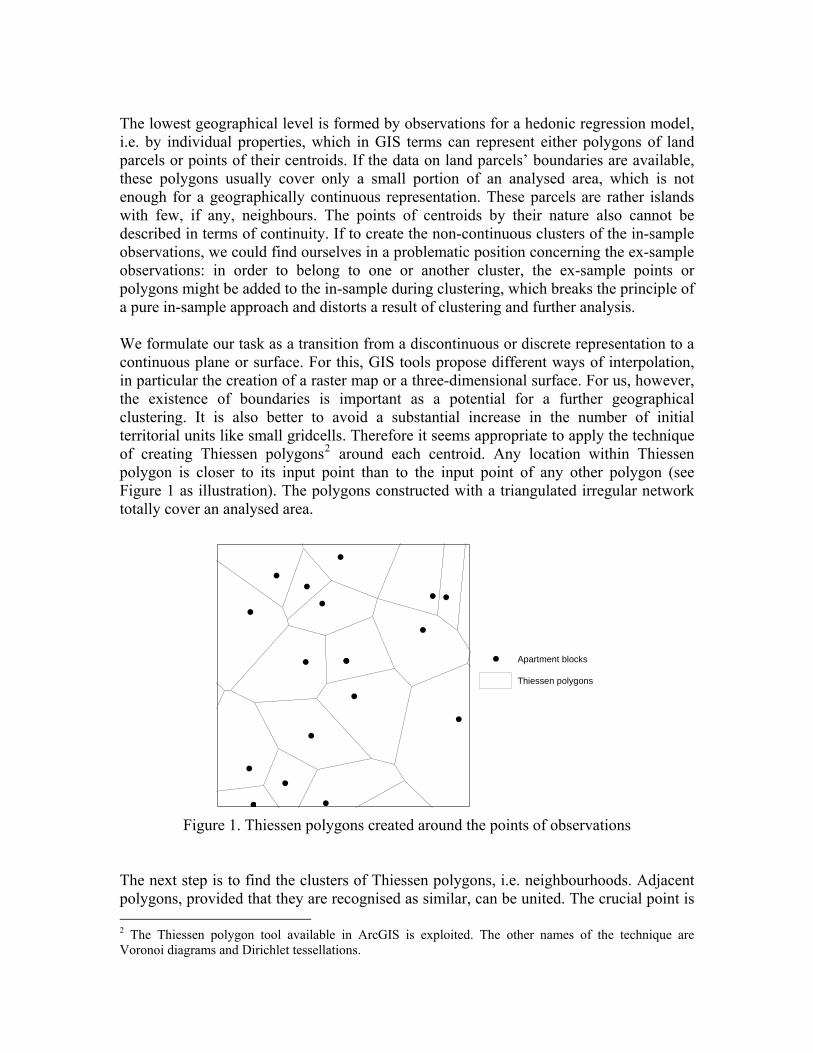
The lowest geographical level is formed by observations for a hedonic regression model, i.e. by individual properties, which in GIS terms can represent either polygons of land parcels or points of their centroids. If the data on land parcels’ boundaries are available, these polygons usually cover only a small portion of an analysed area, which is not enough for a geographically continuous representation. These parcels are rather islands with few, if any, neighbours. The points of centroids by their nature also cannot be described in terms of continuity. If to create the non-continuous clusters of the in-sample observations, we could find ourselves in a problematic position concerning the ex-sample observations: in order to belong to one or another cluster, the ex-sample points or polygons might be added to the in-sample during clustering, which breaks the principle of a pure in-sample approach and distorts a result of clustering and further analysis. We formulate our task as a transition from a discontinuous or discrete representation to a continuous plane or surface. For this, GIS tools propose different ways of interpolation, in particular the creation of a raster map or a three-dimensional surface. For us, however, the existence of boundaries is important as a potential for a further geographical clustering. It is also better to avoid a substantial increase in the number of initial territorial units like small gridcells. Therefore it seems appropriate to apply the technique of creating Thiessen polygons2 around each centroid. Any location within Thiessen polygon is closer to its input point than to the input point of any other polygon (see Figure 1 as illustration). The polygons constructed with a triangulated irregular network totally cover an analysed area.

!

!

!

!

!

!

!

!

!

!

!

!

!

!

!

!!

!

!

! Apartment blocks

Thiessen polygons

Figure 1. Thiessen polygons created around the points of observations

The next step is to find the clusters of Thiessen polygons, i.e. neighbourhoods. Adjacent polygons, provided that they are recognised as similar, can be united. The crucial point is 2 The Thiessen polygon tool available in ArcGIS is exploited. The other names of the technique are Voronoi diagrams and Dirichlet tessellations.

a measure of similarity. For this, we propose to apply a fuzzy sets theory and calculate a fuzzy equality of the attributes of polygons. In fuzzy sets, a membership function is specified as a continuous range [0,1], not (0,1) as for crisp sets. With normalizing, crisp inputs for attributes are converted to the values of a fuzzy membership function. For example, the attribute “population” ranging from 10 to 100 inhabitants for different polygons can be converted into the fuzzy membership function “highly populated” with the minimum of 0 (for polygon with 10 inhabitants) and the maximum of 1 (for polygon with 100 inhabitants). After this simple fuzzyfication the polygons are represented as fuzzy sets. The formal view of a fuzzy set A~ is the following:

{ }xxA A /)(~ μ= , where x – attribute,

)(xAμ – membership function, [ ]1,0)( ∈xAμ .

Fuzzy set can consist of multiple attributes x characterising polygons. Melikhov et al. (1990) describe the following measure of fuzzy equality of two fuzzy sets A~ and B~ :

))()(&()~,~( xxBA BA μμμ ↔= , where – equivalence, ↔ )),1max(),,1min(max( cddcdc −−=↔ ; & – conjunction, . ),min(& dcdc = If then the sets 5.0)~,~( ≥BAμ A~ and B~ are fuzzy equal3. The property of transitivity allows finding more than two fuzzy equal sets that in our case means uniting into clusters more than two polygons. Our additional condition of uniting two polygons is their adjacency, i.e. existence of a common boundary. Thus, if adjacent polygons are fuzzy equal, they are united. The algorithm starts with the highest fuzzy equality among all the adjacent cases. A number of clusters is determined by the technique itself. This can be regarded as an advantage in comparison with the widely applied Ward’s and K-means algorithms (see e.g. Bourassa et al., 1999 or Wilhelmsson, 2004). On the other hand, the proposed technique is completely based on the fuzzy equality measure and does not account for statistical verification. Using this algorithm, a GIS script for clustering has been created. The algorithm can be applied iteratively, with creating bigger neighbourhoods from smaller ones, which corresponds to their hierarchical nature. The process stops when no more fuzzy equal sets are found among adjacent polygons.

3 In this application, we do not consider the case of equality to 0.5, i.e. fuzzy indifference, as fuzzy equality.

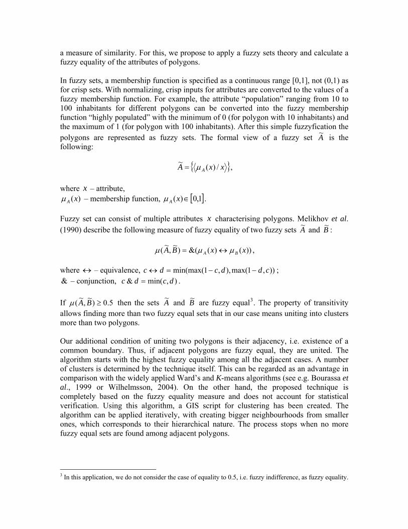
4. Data This study analyses the apartment market in Lyon and Villeurbanne. These adjacent cities with overall population of over 600 thousand inhabitants have a common planning structure and transportation network and make up the core of the Lyon Urban Area, which is the second largest agglomeration by population in France. More detailed description of the apartment market can be found in Bonnafous and Kryvobokov (2011). Administratively, Lyon is divided into nine arrondissements, whose numbers are presented in Figure 2, while Villeurbanne does not have such division. Villeurbanne as a whole and arrondissements of Lyon are hereafter referred to as municipalities. At the lower level, in the study area there are 230 IRISes4 – statistical units, used also as traffic analysis zones; for short, they are referred to as zones.

7

9

3

8

5

64

2

1 Villeurbanne

0 1 20.5 Kilometers

Boundary of Lyon and Villeurbanne

Arrondissements

Centroids of apartment blocks

15 centres

±

Figure 2. Location of the in-sample apartments

The Perval dataset is used, which contains the data on apartment sales in Lyon and Villeurbanne in 1997-2008. The observations with missing data, with prices lower than 20,000 euros and higher than 500,000 euros, with area less than 20 square metres and more than 200 square metres were deleted. The sample consists of 3,159 apartments. This

4 Les îlots regroupés pour l’information statistique.

sample is randomly divided into two parts: the in-sample (80%, 2,527 observations) (Figure 2) and the ex-sample (20%, 632 observations). We use years of transaction as dummies, structural variables and location attributes. The definitions of apartment variables and their description for the in-sample are presented in Table 1. Distribution of sales by years varies from 2% for 1997 to 14% for 2002. Structure is described with the attributes of building age, apartment area, dummies for floor, number of bathrooms, number of parking places, state of apartment, quality of view, number of cellars, and existence of garden and terrace. Number of rooms is not described, because their dummies are highly correlated with apartment area and are insignificant if included in the hedonic model. Building age is estimated as follows. There are seven construction periods available: before 1850; 1850-1913; 1914-1947; 1948-1969; 1970-1980; 1981-1991; and 1992 and later. We assume that a mean for the first construction period is 1800 and for the last period is 2000 and calculate the variable Building_Age as a difference between the year 2000 and the means of the earlier periods. For example, Building_Age for the second period is equal to 2000-1882=118. In the in-sample, 93% of the apartments have one bathroom, while three bathrooms exist in less than 1% of apartments. As much as 82% of apartments are described in the Perval database as having good state. For half of apartments, the existence of one parking pace is reported. Many observations contain no data about the number of parking places and quality of view; therefore, the specific dummy variables are created. The location attributes (Table 2) include the socio-geographical attributes of the percentages of low- and high-income households in zones and travel times to urban centres in minutes. The income groups are composed each of the 20% households in the income range with the lowest and the highest income respectively. Travel times for the travel by car between zones in the morning peak were obtained from the MOSART5 transportation model for the Lyon Urban Area. Travel times to fifteen service employment centres of Lyon and Villeurbanne (Figure 2) are used. These centres have been formally identified in Kryvobokov (2010).

5 Modélisation et Simulation de l’Accessibilité aux Réseaux et aux Territoires (Modelling and Simulation of Accessibility to Networks and Territories).

Table 1. Definitions of apartment variables and descriptive statistics Variable Description Mean Minimum Maximum Std. dev.

Price Transaction price, euro 127,243 20,000 500,000 72,374 Year97 - Year08 Dummies for year of

transaction 0.02-0.14 0 1 0.13 - 0.35

Building_Age Building age, years 36.01 0 200 47.41 Area Apartment area, square

metres 68.44 20 196 26.98

FloorGround Dummy for ground floor

0.12 0 1 0.32

Floor1 Dummy for storey 1 0.18 0 1 0.38 Floor2_8 Dummy for storey 2 to

8 0.68 0 1 0.47

Floor9+ Dummy for storey 9 and more

0.02 0 1 0.14

Bath1 - Bath3 Dummies for number of bathrooms

<0.01 - 0.93 0 1 0.04 - 0.26

Park_Unknown Dummy for cases with no data about parking places

0.33 0 1 0.47

Park0 - Park3 Dummies for number of parking places

<0.01 - 0.50

0 1 0.06 - 0.50

Cond_Good Dummy for good state 0.82 0 1 0.39 Cond_Med Dummy for state when

some maintenance is needed

0.15 0 1 0.36

Cond_Bad Dummy for state when renovation is needed

0.03 0 1 0.18

View_Unknown Dummy for cases with no data about view

0.61 0 1 0.49

View_Good Dummy for view increasing value

0.37 0 1 0.48

View_Bad Dummy for vies decreasing value

0.02 0 1 0.14

Cellar0 – Cellar2

Dummies for number of cellars

0.02 - 0.34 0 1 0.14 - 0.48

Garden Dummy for garden 0.05 0 1 0.21 Terrace Dummy for terrace 0.09 0 1 0.28

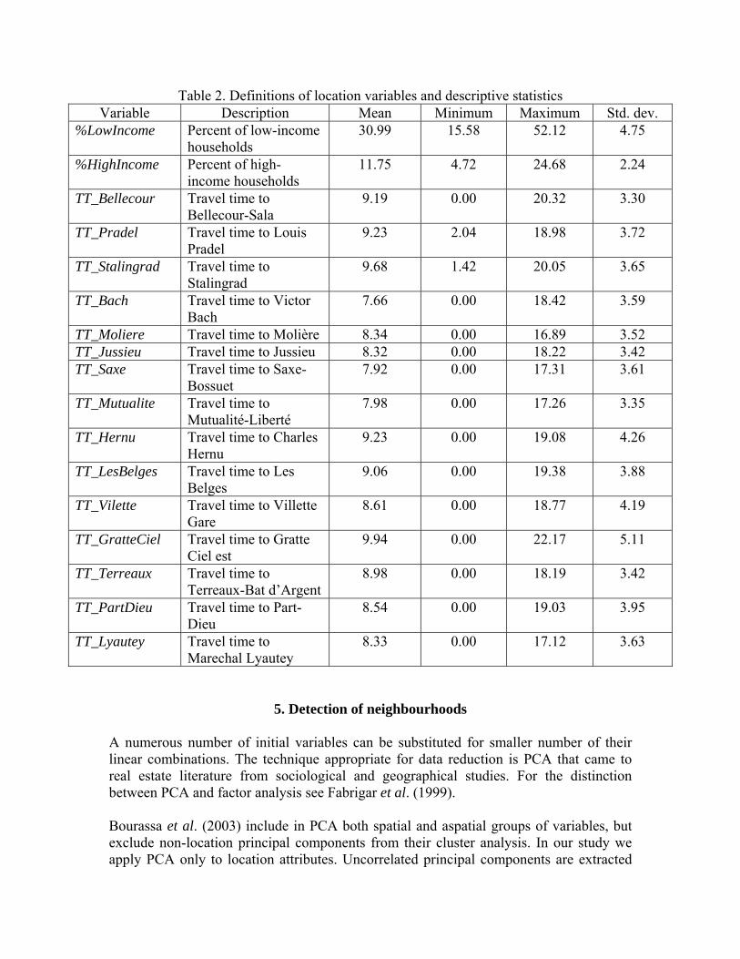
Table 2. Definitions of location variables and descriptive statistics Variable Description Mean Minimum Maximum Std. dev.

%LowIncome Percent of low-income households

30.99 15.58 52.12 4.75

%HighIncome Percent of high-income households

11.75 4.72 24.68 2.24

TT_Bellecour Travel time to Bellecour-Sala

9.19 0.00 20.32 3.30

TT_Pradel Travel time to Louis Pradel

9.23 2.04 18.98 3.72

TT_Stalingrad Travel time to Stalingrad

9.68 1.42 20.05 3.65

TT_Bach Travel time to Victor Bach

7.66 0.00 18.42 3.59

TT_Moliere Travel time to Molière 8.34 0.00 16.89 3.52 TT_Jussieu Travel time to Jussieu 8.32 0.00 18.22 3.42 TT_Saxe Travel time to Saxe-

Bossuet 7.92 0.00 17.31 3.61

TT_Mutualite Travel time to Mutualité-Liberté

7.98 0.00 17.26 3.35

TT_Hernu Travel time to Charles Hernu

9.23 0.00 19.08 4.26

TT_LesBelges Travel time to Les Belges

9.06 0.00 19.38 3.88

TT_Vilette Travel time to Villette Gare

8.61 0.00 18.77 4.19

TT_GratteCiel Travel time to Gratte Ciel est

9.94 0.00 22.17 5.11

TT_Terreaux Travel time to Terreaux-Bat d’Argent

8.98 0.00 18.19 3.42

TT_PartDieu Travel time to Part-Dieu

8.54 0.00 19.03 3.95

TT_Lyautey Travel time to Marechal Lyautey

8.33 0.00 17.12 3.63

5. Detection of neighbourhoods A numerous number of initial variables can be substituted for smaller number of their linear combinations. The technique appropriate for data reduction is PCA that came to real estate literature from sociological and geographical studies. For the distinction between PCA and factor analysis see Fabrigar et al. (1999). Bourassa et al. (2003) include in PCA both spatial and aspatial groups of variables, but exclude non-location principal components from their cluster analysis. In our study we apply PCA only to location attributes. Uncorrelated principal components are extracted

with Varimax orthogonal rotation. The non-collinear components with eigenvalues higher than unity are applied in cluster analysis. PCA is applied at the three geographical levels: individual apartments, zones, and municipalities. For apartments, eighteen initial variables are analysed: travel times to the fifteen centres, %LowIncome, %HighIncome, and Building_Age. While building age refers to an apartment block, the data on other attributes were collected at the level of zones. Thus, dependency from the existing boundaries still exists. The extracted principal components are described in Table 36. Four principal components with eigenvalues higher than unity are extracted, which account for more than 80% of the variance. Added to the OLS regression instead of the location variables (see Section 6), components 1, 3 and 4 demonstrate significance. These three components are used in clustering. At higher geographical levels, building age is excluded as an attribute of apartment block. Average building age in zones and municipalities is not calculated due to the lack of comprehensive data. At the level of zones, seventeen location variables are analysed: travel times to fifteen centres, %LowIncome, and %HighIncome. We extracted four principal components (Table 3), of which the first two account for more than 80% of the variance. Components 1, 3 and 4 demonstrating significance in OLS regression are exploited in formation of clusters. For municipalities, seven location variables are analysed by PCA: travel times to five municipalities, where the service employment centres are located (the Lyon arrondissements 1, 2, 3 and 6, and Villeurbanne), and two income groups. Three principal components are extracted (Table 3), which account for more than 80% of the variance. All three components are significant and used in clustering. In the clustering process, we use polygons and take into account the principal components of location variables. This allows forming continuous clusters covering the whole analysed area and characterised by geographical attributes. Thus, each ex-sample observation unambiguously belongs to one or another geographical cluster and shares its attributes. The clustering process is iterative, i.e. the clusters formed in the initial step are considered in the next clustering step as polygons with average weighted values of attributes (principal components’ scores) with areas of initial polygons used as weights.

6 The scores of principal components are interpolated to raster to see their spatial distribution; the maps are not presented in the paper. For similar maps, see Bonnafous and Kryvobokov (2011).

Table 3. Description of principal components Principal

components Apartments Zones Municipalities

Principal component

1

New accommodation located farther from centres, but not obviously very far from the centres of Villeurbanne, positively correlated with high-income households and negatively correlated with low-income variable, both correlations are 21.5%.

Located farther from centres (with one exception for Villeurbanne), weakly positively correlated with high-income households.

Located farther from centres (with the exception for Villeurbanne), weakly negatively correlated with both income groups.

Principal component

2

Rather older accommodation, though correlation with building age is only 17.5%, located farther from the centres of Villeurbanne and eastern Lyon, weakly positively correlated with high-income households and weakly negatively correlated with low-income variable.

Located mainly in the western part of Lyon closer to arrondissement 2 than to other centres, insignificant correlation with income groups.

Rich population (as opposed to poor households), for whom travel times to centres are in general not very important. They are located rather closer to arrondissement 6 and farther from the other centres of Lyon.

Principal component

3

Rather older buildings, though correlation with building age is only 10%, located farther from the centres of Lyon, but not obviously very far from the centres of Villeurbanne, positively correlated with high-income households (20%) and negatively correlated with low-income variable (26%).

Located farther from the majority of centres of Lyon, but insignificantly or negatively correlated with travel times to the centres of Villeurbanne, weakly positively correlated with high-income households. The minimum of its score is located in Guillotière7, which forms the core of its spatial distribution.

Positively correlated with both income groups, though the coefficient is higher for high-income households (26.2%), located closer to Villeurbanne and farther from arrondissements 1 and 2.

Principal component

4

Rich population (as opposed to poor households) in newer accommodation (correlation 25.6%), for whom travel times to centres are not very important. They are located rather farther from the main centres of Lyon.

Rich population (as opposed to poor households), for whom travel times to centres are not important. They are located rather farther from the main centres of Lyon, mainly in the northern and western directions.

7 A problematic low-income area located remarkably close to the centre of Lyon, populated by immigrants and being the object of the specific attention of the police.

Geographically, each apartment is represented as a point of centroid of an apartment block, where it is located. Around 2,527 apartments we construct 1,689 Thiessen polygons. There are two reasons of the smaller number of polygons. First, many apartments are located in the same apartment blocks and therefore share the same centroids. Second, some apartments might be sold more than once, but this information is not available. All the apartments within a particular block are characterised by the same location variables used to construct their principal components. The clustering process is reported in Table 4, which contains the number of initial territorial unit, clusters and iterations. From 10 municipalities, 6 clusters are formed after the first iteration, and no more clusters are found. Zones are united into 9 clusters after 9 iterations, when the process is finished. We also use the intermediate version of 44 zone clusters formed after 3 iterations (see Figure 3) to have a number of neighbourhoods similar to that created with apartments’ Thiessen polygons.

Table 4. Clustering Thiessen polygons

Number Lyon West

Lyon Peninsula

Lyon East Villeurbanne Zones Municipa-

lities

Initial units 255 310 871 253 230 10

25 27 71 12 Clusters of principal

components 43 44 9 6

8 10 14 12 Iterations 10

3 9 1

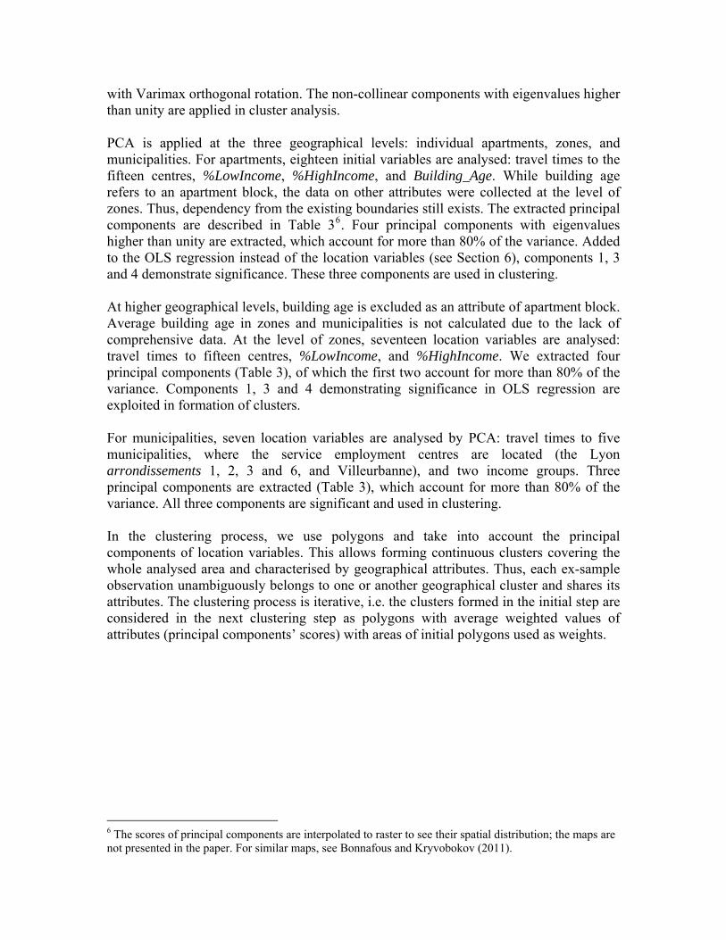
Because the number of Thiessen polygons exceeds limitation existing in our clustering script, these polygons are divided into four geographical parts. In terms of Clapp and Wang (2006), who distinguish between hard and soft boundaries, we use the former type: geographical barriers and administrative limits. Thus, Villeurbanne is analysed separately as a whole, while Lyon is divided into three parts by two rivers: Lyon West is composed by arrondissements 5 and 9 on the right bank of the Saône, Lyon East consists of arrondissements 6, 3, 7 and 8 on the left bank of the Rhône, and Lyon Peninsula is arrndissements 4, 1 and 2 between the rivers. Clustering takes place independently in each part. For example, in Lyon West after 8 iterations, 25 clusters are found. Afterwards all the formed 135 clusters are analysed together and after 10 iterations they form 66 clusters. Small enclaves containing less than 5 apartments are merged with surrounding clusters decreasing the number of neighbourhoods to 43 (Figure 3).

0 1 20.5 Kilometers

Spatial error estimate:

Negative

Insignificant

Positive

Reference

No observations

43 clusters of Thiessen polygons 44 clusters of zones

Figure 3. Neighbourhoods: clusters of Thiessen polygons and zones

6. Hedonic price model

Theory provides no guide concerning the functional form of a hedonic regression model. We apply the log-log specification with dummies. The dependent variable is the log of Price. The log transformations of Area, Building_Age, %LowIncome and travel times are used. The variable %HighIncome is found insignificant probably due to small percentage of population belonging to the high-income group. The dummies Year97, FloorGround, Bath1, Park0, Cond_Good, View_Good and Cellar0 are default values. The OLS methodology is exploited in the beginning. However, when observations are spatially dependent, which is always the case for real estate prices, OLS estimates are inefficient and inconsistent (Dubin, 1998), while the estimate of the variance is biased (Anselin, 1988). The importance of these issues should be considered, even though in this study we do not focus on individual coefficients. The GWR technique (Brunsdon et al., 1996) has a powerful potential able to solve regression equations individually in each observation. In this paper, however, GWR is not applied due to a trivial reason that the number of variables in our model (with too many dummies for neighbourhoods) exceeds limitation in the available software.

In Clapp’s local regression and Case’s model with submarkets in Case et al. (2004), nearest neighbour residuals are under special attention. Their conclusion is that the nearest neighbour residuals containing the information on the value of unobserved property and neighbourhood attributes should be included in the model if the purpose is to predict ex-sample. The spatial error methodology, where the error term is a function of the errors in nearby areas, explicitly accounts for this issue. We apply this technique, which, unlike the methodology of dependent variable’s spatial lag, provides a straightforward interpretation of coefficients as partial derivatives of a dependent variable. Eight model specifications are examined with the OLS and spatial error techniques. The baseline model does not contain any location attributes; construction period is not included either due to high correlation with location. The “trend surface analysis” variables of coordinates X and Y of apartment blocks’ centoids as well as %LowIncome and Building_Age are included in the next model; we cannot add X-squared and Y-squared to this specification due to enormous multicollinearity. The other alternative without neighbourhoods contains four additional variables (hereafter referred to as “four location variables”): travel times to two service employment centres TT_Bellecour and TT_Pradel (with whom the model fit reaches its maximum), percentage of low-income households, and building age. In line with the argument of Ross et al. (2009), we are unable to include more than travel time variables. There are five models with different versions of neighbourhoods: municipalities, clusters of Thiessen polygons, two versions of clusters of zones, and clusters of municipalities (see Table 4). The two alternatives of zone clusters are included to examine their influence at both lower and upper geographical levels: the number of clusters of the former level (44) is comparable with the number of Thiessen polygons’ clusters (43), whereas the number of clusters of the latter (9) is similar to the number of municipalities (10). Thus, with approximately the same number of neighbourhoods created from points or zones in one case and from zones and municipalities in the other we can verify if it is worth starting clustering from lower geographical level. In all the cases, the default neighbourhood is that, where the Lyon city hall is located. The specifications with neighbourhoods include the variables from the baseline model and building age. The other location variables are excluded to decrease multicollinearity and allow spatial effects to be better captured by the spatial error technique8. For all the models, a Jarque-Bera test (OLS) and a Breusch-Pagan test (OLS and spatial error) indicate no rejection of the assumptions of normality and heteroskedasticity. Table 5 exhibits the estimates9 of the baseline model without location variables and of the three models with dummies for neighbourhoods: municipalities, 43 clusters of Thiessen polygons, and 44 clusters of zones. Neighbourhood variables are not presented because of their large number; instead, we report their number (except the default

8 Spatial error specifications with neighbourhoods, two travel times and percentage of low-income households demonstrate the tendency of prediction similar to the reported one. 9 Table 5 contains the estimates significant at the 5% level in at least one model; t-values for OLS and asymptotic t-values for spatial error models are in parentheses.

dummy) and the percentages significant at the 5% level or better. In case of zones, there are less neighbourhood dummies than clusters, because some clusters do not contain sales. When municipalities and building age are added to the OLS baseline model, three structural attributes (Bath3, Park_Unknown and Garden) become insignificant, the rest behave in the same manner as before. The clusters of Thiessen polygons and zones applied instead of municipalities do not substantially change other significant estimates except Cellar1, which becomes insignificant in the latter case. In comparison with the OLS, in the spatial error specification of the baseline model, the coefficients for dummies for years of sales are slightly increased, while the estimates for structural attributes are mainly decreased, some of them become insignificant. The specifications with neighbourhoods in this respect, in general, behave similarly, but the tendency of increasing the dummies for years and decreasing the structural variables is not always observed, especially for the clusters of Thiessen polygons and zones. Among the OLS models, the highest percentage of significant neighbourhood dummies, 84, belongs for the clusters of zones. This percentage is similar to 86 from Case et al. (2004). With spatial error technique, the number of significant dummies for municipality decreases from seven to five in comparison with the OLS; for clusters of Thiessen polygons this number decreases in almost two times, but the most visible fall, in 3.5 times, is observed for the significant clusters of zones. The maps of clusters created from Thiessen polygons and zones, presented in Figure 3, distinguish between neighbourhoods, positively and negatively influencing prices in the spatial error equations. The main difference between the two versions is that the clusters of Thiessen polygons located to the north from the reference cluster positively influence sale prices, while the clusters of zones to the north-west from their reference have negative influence. This can be explained by a large size of the reference cluster of Thiessen polygons, which includes not only the very central part of Lyon, but also some surrounding areas; in the case of zone clusters, on the contrary, the reference neighbourhood is relatively small, moreover, the prestigious areas to the north from the reference are united with some less desirable areas of neighbouring arrondissements.

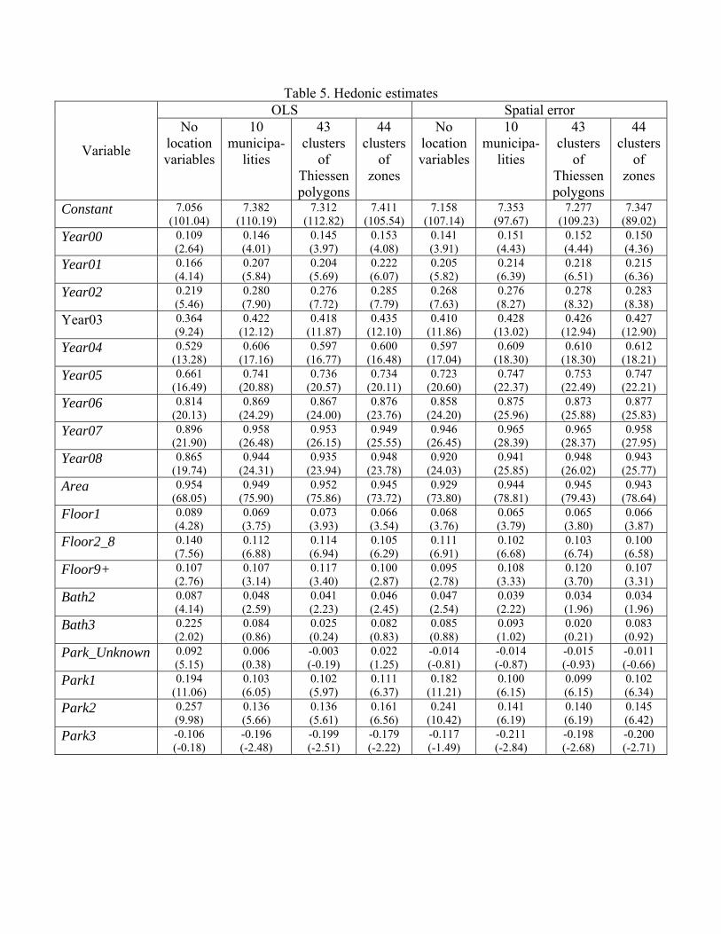
Table 5. Hedonic estimates OLS Spatial error

Variable

No location variables

10 municipa-

lities

43 clusters

of Thiessen polygons

44 clusters

of zones

No location variables

10 municipa-

lities

43 clusters

of Thiessen polygons

44 clusters

of zones

Constant 7.056 (101.04)

7.382 (110.19)

7.312 (112.82)

7.411 (105.54)

7.158 (107.14)

7.353 (97.67)

7.277 (109.23)

7.347 (89.02)

Year00 0.109 (2.64)

0.146 (4.01)

0.145 (3.97)

0.153 (4.08)

0.141 (3.91)

0.151 (4.43)

0.152 (4.44)

0.150 (4.36)

Year01 0.166 (4.14)

0.207 (5.84)

0.204 (5.69)

0.222 (6.07)

0.205 (5.82)

0.214 (6.39)

0.218 (6.51)

0.215 (6.36)

Year02 0.219 (5.46)

0.280 (7.90)

0.276 (7.72)

0.285 (7.79)

0.268 (7.63)

0.276 (8.27)

0.278 (8.32)

0.283 (8.38)

Year03 0.364 (9.24)

0.422 (12.12)

0.418 (11.87)

0.435 (12.10)

0.410 (11.86)

0.428 (13.02)

0.426 (12.94)

0.427 (12.90)

Year04 0.529 (13.28)

0.606 (17.16)

0.597 (16.77)

0.600 (16.48)

0.597 (17.04)

0.609 (18.30)

0.610 (18.30)

0.612 (18.21)

Year05 0.661 (16.49)

0.741 (20.88)

0.736 (20.57)

0.734 (20.11)

0.723 (20.60)

0.747 (22.37)

0.753 (22.49)

0.747 (22.21)

Year06 0.814 (20.13)

0.869 (24.29)

0.867 (24.00)

0.876 (23.76)

0.858 (24.20)

0.875 (25.96)

0.873 (25.88)

0.877 (25.83)

Year07 0.896 (21.90)

0.958 (26.48)

0.953 (26.15)

0.949 (25.55)

0.946 (26.45)

0.965 (28.39)

0.965 (28.37)

0.958 (27.95)

Year08 0.865 (19.74)

0.944 (24.31)

0.935 (23.94)

0.948 (23.78)

0.920 (24.03)

0.941 (25.85)

0.948 (26.02)

0.943 (25.77)

Area 0.954 (68.05)

0.949 (75.90)

0.952 (75.86)

0.945 (73.72)

0.929 (73.80)

0.944 (78.81)

0.945 (79.43)

0.943 (78.64)

Floor1 0.089 (4.28)

0.069 (3.75)

0.073 (3.93)

0.066 (3.54)

0.068 (3.76)

0.065 (3.79)

0.065 (3.80)

0.066 (3.87)

Floor2_8 0.140 (7.56)

0.112 (6.88)

0.114 (6.94)

0.105 (6.29)

0.111 (6.91)

0.102 (6.68)

0.103 (6.74)

0.100 (6.58)

Floor9+ 0.107 (2.76)

0.107 (3.14)

0.117 (3.40)

0.100 (2.87)

0.095 (2.78)

0.108 (3.33)

0.120 (3.70)

0.107 (3.31)

Bath2 0.087 (4.14)

0.048 (2.59)

0.041 (2.23)

0.046 (2.45)

0.047 (2.54)

0.039 (2.22)

0.034 (1.96)

0.034 (1.96)

Bath3 0.225 (2.02)

0.084 (0.86)

0.025 (0.24)

0.082 (0.83)

0.085 (0.88)

0.093 (1.02)

0.020 (0.21)

0.083 (0.92)

Park_Unknown 0.092 (5.15)

0.006 (0.38)

-0.003 (-0.19)

0.022 (1.25)

-0.014 (-0.81)

-0.014 (-0.87)

-0.015 (-0.93)

-0.011 (-0.66)

Park1 0.194 (11.06)

0.103 (6.05)

0.102 (5.97)

0.111 (6.37)

0.182 (11.21)

0.100 (6.15)

0.099 (6.15)

0.102 (6.34)

Park2 0.257 (9.98)

0.136 (5.66)

0.136 (5.61)

0.161 (6.56)

0.241 (10.42)

0.141 (6.19)

0.140 (6.19)

0.145 (6.42)

Park3 -0.106 (-0.18)

-0.196 (-2.48)

-0.199 (-2.51)

-0.179 (-2.22)

-0.117 (-1.49)

-0.211 (-2.84)

-0.198 (-2.68)

-0.200 (-2.71)

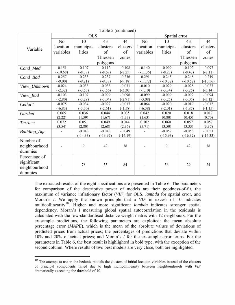
Table 5 (continued) OLS Spatial error

Variable

No location variables

10 municipa-

lities

43 clusters

of Thiessen polygons

44 clusters

of zones

No location variables

10 municipa-

lities

43 clusters

of Thiessen polygons

44 clusters

of zones

Cond_Med -0.151 (-10.68)

-0.107 (-8.37)

-0.112 (-8.67)

-0.108 (-8.25)

-0.140 (-11.36)

-0.099 (-8.27)

-0.102 (-8.47)

-0.097 (-8.11)

Cond_Bad -0.257 (-9.00)

-0.233 (-9.21)

-0.237 (-9.37)

-0.236 (-9.18)

-0.291 (-11.72)

-0.245 (-10.32)

-0.248 (-10.52)

-0.249 (-10.56)

View_Unknown -0.024 (-2.32)

-0.033 (-3.53)

-0.033 (-3.56)

-0.031 (-3.30)

-0.010 (-1.10)

-0.029 (-3.34)

-0.028 (-3.25)

-0.027 (-3.14)

View_Bad -0.103 (-2.80)

-0.107 (-3.29)

-0.099 (-3.04)

-0.096 (-2.91)

-0.099 (-3.08)

-0.099 (-3.25)

-0.092 (-3.05)

-0.094 (-3.12)

Cellar1 -0.075 (-6.83)

-0.034 (-3.30)

-0.027 (-2.61)

-0.017 (-1.58)

-0.064 (-6.38)

-0.020 (-2.01)

-0.019 (-1.87)

-0.012 (-1.15)

Garden 0.065 (2.22)

0.036 (1.39)

0.044 (1.67)

0.035 (1.33)

0.042 (1.63)

0.020 (0.80)

0.018 (0.45)

0.017 (0.70)

Terrace 0.072 (3.54)

0.051 (2.80)

0.049 (2.68)

0.044 (2.36)

0.102 (5.71)

0.060 (3.50)

0.057 (3.33)

0.057 (3.37)

Building_Age - -0.048 (-14.33)

-0.048 (-13.97)

-0.049 (-14.19)

- -0.052 (-15.93)

-0.053 (-16.32)

-0.053 (-16.33)

Number of neighbourhood dummies

- 9 42 38 - 9 42 38

Percentage of significant neighbourhood dummies

- 78 55 84 - 56 29 24

The extracted results of the eight specifications are presented in Table 6. The parameters for comparison of the descriptive power of models are their goodness-of-fit, the maximum of variance inflationary factor (VIF) for OLS, lambda for spatial error, and Moran’s I. We apply the known principle that a VIF in excess of 10 indicates multicollinearity10. Higher and more significant lambda indicates stronger spatial dependency. Moran’s I measuring global spatial autocorrelation in the residuals is calculated with the row-standardised distance weight matrix with 12 neighbours. For the ex-sample predictions, the following parameters are exploited: the mean absolute percentage error (MAPE), which is the mean of the absolute values of deviations of predicted prices from actual prices; the percentages of predictions that deviate within 10% and 20% of actual prices; and Moran’s I for the ex-sample error terms. For the parameters in Table 6, the best result is highlighted in bold type, with the exception of the second column. Where results of two best models are very close, both are highlighted.

10 The attempt to use in the hedonic models the clusters of initial location variables instead of the clusters of principal components failed due to high multicollinearity between neighbourhoods with VIF dramatically exceeding the threshold of 10.

Table 6. Extracted hedonic results Ex-sample prediction

Model

Adjusted R2 (OLS) /

Pseudo R2 (spatial error)

Maximum VIF (OLS) / Lambda

(spatial error)

Moran’s I MAPE

Within 10%

of sale price

Within 20%

of sale price

Moran’s I

OLS models No location variables

0.819 7.933 0.258** 0.1950 35.3 64.2 0.197**

X and Y, no neighbourhoods

0.834 7.966 0.254** 0.1856 36.7 67.4 0.224**

Four location variables, no neighbourhoods

0.859 7.999 0.152** 0.1686 42.4 69.9 0.089**

10 municipalities

0.860 8.027 0.149** 0.1655 42.7 71.8 0.101**

43 clusters of Thiessen polygons

0.861 8.287 0.143** 0.1584 45.3 73.1 0.082**

44 clusters of zones

0.857

8.332 0.156** 0.1635 43.8 71.0 0.080**

9 clusters of zones

0.843 8.010 0.228** 0.1756 39.4 68.5 0.151**

6 clusters of municipalities

0.851 8.007 0.185** 0.1726 42.4 70.3 0.157**

Spatial error models No location variables

0.860 0.833 (31.807)

0.072** 0.1876 34.3 65.7 0.193**

X and Y, no neighbourhoods

0.874 0.847 (34.567)

0.056** 0.1794 37.5 68.4 0.242**

Four location variables, no neighbourhoods

0.874 0.785 (24.823)

0.059** 0.1668 40.0 69.8 0.135**

10 municipalities

0.875 0.765 (22.548)

0.058** 0.1642 40.7 72.0 0.124**

43 clusters of Thiessen polygons

0.878 0.798 (26.414)

0.052* 0.1648 41.1 71.2 0.154**

44 clusters of zones

0.877 0.837 (32.538)

0.046* 0.1711 38.9 67.4 0.197**

9 clusters of zones

0.875 0.867 (39.223)

0.057** 0.1829 35.6 63.6 0.278**

6 clusters of municipalities

0.874 0.815 (28.815)

0.058** 0.1721 38.4 69.1 0.187**

Pseudo-significance for Moran’s I: *p<0.01; **p≤0.001

According to the descriptive power, the best OLS model is that with the clusters of Thiessen polygons, while the second best is that with municipalities. By its performance and spatial autocorrelation of residuals, the OLS model with four location variables and without neighbourhoods is better than the models with zone and municipal clusters. The percentages of prediction of the OLS model with the clusters of Thiessen polygons are the highest. The lowest ex-sample Moran’s I is for 44 zone clusters, but it is almost the same as for the Thiessen polygons’ clusters. Spatial autocorrelation in the OLS residuals is significant, and the application of a spatial technique seems adequate. In the spatial error models, the threshold weight matrix is used, where the threshold is determined such that there is at least one neighbour for each observation11. After accounting for spatial effect, the descriptive power of the model with location variables is no better than that of any model with neighbourhoods. Though the model with the clusters of Thiessen polygons has the highest pseudo R2, it is practically equal to the performance of the model with 44 zone clusters. The letter model also provides the minimum of the spatial autocorrelation in the in-sample residuals; the former model is the second best by this parameter. These are the only two cases where Moran’s I is pseudo-insignificant at the 1% level. The ex-sample predictions for the spatial error models are calculated with an average in-sample residual in each zone. The same zone level is used to calculate average residual by all the models irrespective of whether any neighbourhoods are included and of the geographical level of neighbourhoods. According to predictive power, the situation is different from the OLS. The superiority of the clusters of Thiessen polygons in MAPE and deviations within the 10% prediction interval is contested by the model with municipalities, especially within the 20% interval and by the ex-sample Moran’s I – according to these parameters municipalities provide the best prediction. We should admit that the prediction results of the spatial error models are in most cases worse than those of the OLS. It may reflect the inappropriateness of the selected zone level for calculation of average in-sample residuals. Note that even the spatial models with the clusters of zones do not benefit from the selection of their levels for residuals if to compare their prediction parameters with their OLS counterparts. At the same time, it would be incorrectly to apply for the ex-sample prediction our in-sample weighting scheme with its threshold. In the context of this difficulty of the ex-sample calculation we can mention Wilhelmsson (2004), who notes that spatial regression models are not fully transparent, and therefore it may be problematic to use their results in, for example, property tax assessment. Comparing the models with similar number of neighbourhoods, the following findings can be highlighted. The models with 43 clusters of Thiessen polygons and with 44 zone clusters can be quite similar, especially when the spatial error technique is applied. However, if the neighbourhoods are created from individual observations with Thiessen polygons, the predictive power of this model is stronger according to all the examined parameters. The comparison of the models with 10 municipalities and with 9 clusters of 11 The weighting scheme with a pre-specified number of nearest neighbours does not work for this dataset.

zones differs from the previous finding. The OLS model with municipalities is superior by all the parameters of estimation and prediction. When the spatial errors of both models are accounted for, their estimation results are similar, but the predictive power of the model with municipalities is much higher.

Conclusion This paper proposes a method for defining neighbourhoods applying Thiessen polygons and fuzzy equality clustering. The advantages of the method are that it starts from the lowest level of individual observations, takes into account adjacency, does not need the a priori determination of a number of clusters and can be completely formalised. On the other hand, there is no statistical control in the clustering process. Principal components extracted from location attributes are analysed in the clustering. For the purpose of the study, the influence of the proposed clusters of Thiessen polygons on apartment price is compared with that of other versions of neighbourhoods, which are the clusters of zones and municipalities as well as municipalities themselves. The dummies for neighbourhoods are included in a hedonic regression model. With the OLS technique, the clusters of Thiessen polygons provide the best model in both estimation and prediction aspects. When a model is controlled for spatial error effect, spatial autocorrelation of in-sample residuals is the lowest and pseudo-insignificant at the 1% level at the lowest geographical level: more than forty neighbourhoods are better than ten or less. However, the superiority in the predictive power of the models with the highest geographical resolution is contested by simple municipal division. The difficulty with the ex-sample prediction applying the spatial error methodology complicates the generalisation of our results and implies caution in their interpretation. But if to analyse the spatial error predictions as they are, smaller is not always better. Similarly to Wilhelmsson (2004), we found a limitation in the predictive power when there are too many neighbourhoods, but our finding is different: large administrative units can be better than clusters created at lower geographical levels. The hypothesis that municipalities can be treated as submarkets might be checked in a future study. Thus, the proposed method of neighbourhood delineation could be applied in combination with market segmentation.

Acknowledgements

The study is part of project PLAINSUDD sponsored though French ANR (number ANR-08-VD-00). Provision of data on apartment prices and attributes by Perval and Pierre-Yves Péguy is acknowledged. The author is grateful to Nicolas Ovtracht for calculation of travel times and the coordinates of apartment blocks.

References

Anselin, L. (1988). Spatial econometrics: Methods and models. Dordrecht: Kluwer Academic.

Bonnafous, A. and Kryvobokov, M. (2011). Insight into apartment attributes and location with factors and principal components. International Journal of Housing Markets and Analysis, forthcoming. Borst, R. A. (2007). Discovering and Applying Location Influence Patterns in the Mass Valuation of Domestic Real Property. Doctor of Technology thesis, University of Ulster. Borst, R. A.and McCluskey, W. J. (2008). The Modified Comparable Sales Method as the Basis for a Property Tax Valuation System and its Relationship and Comparison to Spatially Autoregressive Valuation Models, In T. Kauko and M. d’Amato (Eds.), Mass appraisal methods: An international perspective for property valuers. Chichester, UK: Blackwell Publishing. Bourassa, S. C., Cantoni, E., and Hoesli, M. (2007). Spatial Dependence, Housing Submarkets, and House Price Prediction, Journal of Real Estate Finance and Economics, Vol. 35, No 2, pp. 143-160. Bourassa, S. C., Cantoni, E., and Hoesli, M. (2010). Predicting House Prices with Spatial Dependence: A Comparison of Alternative Methods, Journal of Real Estate Research, Vol. 32, No 2, pp. 139-159. Bourassa, S. C., Hamelink, F., Hoesli, M. and MacGregor, B. D. (1999). Defining Housing Submarkets, Journal of Housing Economics, Vol. 8, No. 2, pp. 160-183. Bourassa, S. C., Hoesli, M. and Peng, V. S. (2003). Do housing submarkets really matter?, Journal of Housing Economics, Vol. 12, No 1, pp. 12-28. Brunsdon, C. F., Fotheringham, A. S., and Charlton, M. E. (1996). Geographically Weighted Regression: A Method for Exploring Spatial Nonstationarity, Geographical Analysis, Vol. 28, No 4, pp. 281-298. Case, B., Clapp, J., Dubin, R., and Rodrigues, M. (2004). Modeling Spatial and Temporal House Price Patterns: A Comparison of Four Models, Journal of Real estate Finance and Economics, Vol. 29, No 2, pp. 167-191. Clapp, J. M. and Wang, Y. (2006). Defining neighborhood boundaries: Are census tracts obsolete? Journal of Urban Economics, Vol. 59, No 2, pp. 259-284. Dale-Johnson, D. (1982). An Alternative Approach to Housing Market Segmentation Using Hedonic Price Data, Journal of Urban Economics, Vol. 11, No. 3, pp. 311-332. Des Rosier, F. (1991). RESIVALU: A Hedonic Residential Price Model for the Quebec Region 1986-87, Property Tax Journal, Vol. 10, No 2, pp. 227-255.

Des Rosiers, F., Dubé, J, and Thériault, M. (2010). Do Peer Effects Shape Residential Values? Reconciling the Sales Comparison Approach with Hedonic Price Modelling, 17th Annual European Real Estate Society conference paper, Milan, 23-26 June. Dubé, J. and Legros, D. (2010). A Spatio-Temporal Measure of Spatial Dependence: An Example Using real Estate Data, 57th Annual North American Meetings of the Regional Science Association International, Denver, 10-13 November. Dubin, R. A. (1992). Spatial autocorrelation and neighbourhood quality, Regional Science and Urban Economics, Vol. 22, No 3, pp. 433-452. Dubin, R. A. (1998). Spatial autocorrelation: A primer, Journal of Housing Economics, Vol. 7, No 4, pp. 304-327. Dubin, R. (2003). Robustness of Spatial Autocorrelation Specifications: Some Monte Carlo Evidence, Journal of Regional Science, Vol. 43, No 2, pp. 221-248. Fabrigar, L. R., Wegener, D. T., MacCallum, R. C., and Strahan, E. J. (1999). Evaluating the Use of Exploratory Factor Analysis in Psychological Research, Psychological Methods, Vol. 4, No 3, pp. 272-299. Figueroa, R. A. (1999). Modeling the Value of Location in Regina Using GIS and Spatial Autocorrelation Statistics, Assessment Journal, Vol. 6, No 6, pp. 32-36. Fletcher, M., Gallimore, P., and Mangan, J. (2000). The modeling of housing submarkets, Journal of Property Investment and Finance, Vol. 18, No 42, pp. 473-487. Fuller, L. and Huang, C.-Y. (2003). Determining Market Areas for Multiple Regression Analysis Modeling in the City of Saskatoon, Assessment Journal, Vol. 10, No 3, pp. 41-46. González, M. A. S. (2008). Developing mass appraisal models with fuzzy systems, In T. Kauko and M. d’Amato (Eds.), Mass appraisal methods: An international perspective for property valuers. Chichester, UK: Blackwell Publishing. González, M. A. S. and Formoso, C. T. (2006). Mass appraisal with genetic fuzzy rule-based systems, Property Management, Vol. 24, No 1, pp. 20-30. Goodman, A. C. and Thibodeau, T. G. (1998). Housing Market Segmentation, Journal of Housing Economics, Vol. 7, No 2, pp. 121-143. Goodman, A. C. and Thibodeau, T. G. (2003). Housing market segmentation and hedonic prediction accuracy, Journal of Housing Economics, Vol. 12, No 3, pp. 181-201. Gouriéroux, C. and Laferrère, A. (2009). Managing hedonic housing price indexes: The French experience, Journal of Housing Economics, Vol. 18, No 3, pp. 206-213.

Jenkins, D. H., Lewis, O. M., Almond, N., Gronow, S. A., and Ware, J. A. (1998). Towards an Intelligent Residential Appraisal Model, Journal of Property Research, Vol. 16, No 1, pp. 67-90. Kauko, T. (2003). On Current Neural Network Applications Involving Spatial Modelling of Property Prices, Journal of Housing and the Built Environment, Vol. 18, No 2, pp. 159-181. Kryvobokov, M. (2010). Is it worth identifying service employment (sub)centres when modelling apartment prices? Journal of Property Research, Vol. 27, No 4, pp. 337-356. Lewis, O. M., Ware, J. A., and Jenkins, D. H. (2001). Identification of Residential Property Sub-Markets using Evolutionary and Neural Computing Techniques, Neural Computing & Applications, Vol. 10, No 2, pp. 108-119. Maclennan, D. and Tu, Y. (1996). Economic perspectives on the structure of local housing systems, Housing Studies, Vol. 11, No. 3, pp. 387-406. Melikhov, A. N., Bernshtein, L. S., and Korovin, S. J. (1990). Situation advice systems with fuzzy logic (in Russian). Moscow: Nauka. Pendleton, W. C. (1965). Statistical Inference in Appraisal and Assessment Processes, Appraisal Journal, Vol. 33, No 1, pp. 73-82. Rosen, S. (1974). Hedonic Prices and Implicit Markets: Product Differentiation in Pure Competition, Journal of Political Economy, Vol. 82, No 1, pp. 34-55. Ross, J. M., Farmer, M. C., and Lipscomb, C. A. (2009). Inconsistency in Welfare Inferences from Distance Variables in Hedonic Regressions, Journal of Real Estate Finance and Economics, manuscript published online, 16 p. Smith, R. M. (1986). Comparing Traditional Methods for Selecting Class Intervals on Choropleth Maps, Professional Geographer, Vol. 38, No 1, pp. 62-67. Ward, R. D., Guilford, J., Jones, B., Pratt, D., and German, J. C. (2002). Piecing together location: three studies by the Lucas county research and development staff, Assessment Journal, Vol. 9, No 5, pp. 15-48. Watkins, C. A. (2001). The definition and identification of housing submarkets, Environment and Planning A, Vol. 33, No 12, pp. 2235-2253. Wilhelmsson, M. (2004). A method to derive housing sub-markets and reduce spatial dependency, Property Management, Vol. 22, No 4, pp. 276-288.