Defining and Controlling the Heterogeneity of a … · Defining and Controlling the Heterogeneity...

HAL Id: inria-00438616https://hal.inria.fr/inria-00438616

Submitted on 4 Dec 2009

HAL is a multi-disciplinary open accessarchive for the deposit and dissemination of sci-entific research documents, whether they are pub-lished or not. The documents may come fromteaching and research institutions in France orabroad, or from public or private research centers.

L’archive ouverte pluridisciplinaire HAL, estdestinée au dépôt et à la diffusion de documentsscientifiques de niveau recherche, publiés ou non,émanant des établissements d’enseignement et derecherche français ou étrangers, des laboratoirespublics ou privés.

Defining and Controlling the Heterogeneity of a Cluster:the Wrekavoc Tool

Louis-Claude Canon, Olivier Dubuisson, Jens Gustedt, Emmanuel Jeannot

To cite this version:Louis-Claude Canon, Olivier Dubuisson, Jens Gustedt, Emmanuel Jeannot. Defining and Controllingthe Heterogeneity of a Cluster: the Wrekavoc Tool. Journal of Systems and Software, Elsevier, 2010,83 (5), pp.786-802. <10.1016/j.jss.2009.11.734>. <inria-00438616>

https://hal.inria.fr/inria-00438616

https://hal.archives-ouvertes.fr

appor t

de r ech er ch e

ISS

N0

24

9-6

39

9IS

RN

INR

IA/R

R--

71

35

--F

R+

EN

G

Domaine 3

INSTITUT NATIONAL DE RECHERCHE EN INFORMATIQUE ET EN AUTOMATIQUE

Defining and Controlling the Heterogeneity of a

Cluster: the Wrekavoc Tool

Louis-Claude Canon — Olivier Dubuisson — Jens Gustedt — Emmanuel Jeannot

N° 7135

December 2009

Centre de recherche INRIA Nancy – Grand EstLORIA, Technopôle de Nancy-Brabois, Campus scientifique,

615, rue du Jardin Botanique, BP 101, 54602 Villers-Lès-NancyTéléphone : +33 3 83 59 30 00 — Télécopie : +33 3 83 27 83 19

Defining and Controlling the Heterogeneity of a

Cluster: the Wrekavoc Tool

Louis-Claude Canon∗† ‡ , Olivier Dubuisson§† , Jens Gustedt† ,Emmanuel Jeannot†‡

Domaine : Reseaux, systemes et services, calcul distribueEquipes-Projets AlGorille and Runtime

Rapport de recherche n° 7135 — December 2009 — 38 pages

Abstract: The experimental validation and the testing of solutions that are designedfor heterogeneous environments is challenging. We introduce Wrekavoc as an accuratetool for this purpose: it runs unmodified applications on emulated multisite heteroge-neous platforms. Its principal technique consists in downgrading the performance ofthe platform characteristics in a prescribed way. The platform characteristics includethe compute nodes themselves (CPU and memory) and the interconnection network forwhich a controlled overlay network above the homogeneous cluster is built. In this arti-cle we describe the tool, its performance, its accuracy and its scalability. Results showthat Wrekavoc is a very versatile tool that is useful to perform high-quality experiments(in terms of reproducibility, realism, control, etc.)

Key-words: Tool for experimentation, performance modeling, emulation, heteroge-neous systems

This paper has been accepted for publication Journal of Systems and Software.

∗ Nancy University† AlGorille Team, INRIA Nancy – Grand Est‡ Runtime Team, INRIA Bordeaux – Sud-Ouest§ Felix Informatique

Definir et controler l’heterogeneıte d’une grappe :

l’outil Wrekavoc

Resume : La validation experimentale et le test de solutions qui ont ete concuespour des environnements heterogenes est un veritable defi. A cette fin, nous intro-duisons Wrekavoc, dont l’objectif est de repondre a ce probleme de maniere precise, enexecutant des applications non modifiees sur des plates-formes multi-sites heterogenesemulees. La principale technique employee consiste a degrader de maniere predefinieles caracteristiques de la plate-forme utilisee. Les caracteristiques concernees sont :les nœuds de calcul eux-memes (CPU et memoire) et le reseau d’interconnexion pourlequel un overlay est definit et construit au dessus de la grappe homogene consideree.Dans cet article nous decrivons l’outil, sa performance, sa precision et son extensi-bilite. Les resultats montrent que Wrekavoc est un outil tres versatile qui est utilepour effectuer des experiences de haute qualite en termes de reproductibilite, realisme,controle, etc.

Mots-cles : outil pour l’experience, modelisation de la performance, emulation, sys-temes heterogenes

Defining and Controlling the Heterogeneity of a Cluster: the Wrekavoc Tool 3

1 Introduction

Distributed computing and distributed systems is a branch of computer science that hasrecently gained very large attention. Grids [1], clusters of clusters [2], peer-to-peersystems [3, 4], desktop environments [5, 6], are examples of successful environmentson which applications (scientific, data managements, etc.) are executed routinely.

However, such environments are composed of a multitude of different elementsthat make them more and more complex. The hardware (from CPU cores to inter-connected clusters) is hierarchical and heterogeneous. Programs that are executed onthese infrastructures can be composite and extremely elaborate. Huge amounts of data,possibly scattered on different sites, are processed. Numerous protocols are used tointer-operate the different parts of these environments. Networks that interconnect thedifferent hardware are also heterogeneous and multi-protocol.

As a consequence, applications (and the algorithms implemented by them) areequally complex and become very hard to validate. However, validation is of keyimportance for application software: it assesses the correctness and the efficiency ofthe proposed solution, and allows for the comparison of a given solution to other al-ready existing ones. Analytic validation consists in modeling the problem space, theenvironment and the solution. Its goal is then to gather knowledge about the modeledbehavior using mathematics. For the domain that we are investigating here, analyticvalidation is often infeasible due to the complexity and partial unpredictability of thestudied objects.

It is therefore mandatory to switch to experimental validation. This consists inexecuting the application (or a model of it), observing its behavior on different casesand comparing it with other solutions. This necessity for experiments truly makes thisfield of computer science an experimental science.

As in every experimental science, experiments are made through the means of toolsand instruments. In computer science one can distinguish different methodologiesfor performing experiments, namely, benchmarking, real-scale, simulation and emu-lation [7].

Here, we describe a new emulator called Wrekavoc. The goal of Wrekavoc is totransform a homogeneous cluster into a multi-site distributed heterogeneous environ-ment. This is achieved by degrading the perceived performance of the hardware bymeans of software that is run at user level. Then, using this emulated environment areal unmodified program can be executed to test and compare it with other solutions.Building such a tool is a scientific challenge: it requires to establish links between re-ality and models. Such models need to be validated in order to understand their limitsand to assess their realism. However, a brief look at the literature shows that concern-ing simulators [8, 9] or emulators [10, 11], the validation of the proposed tools (endhence the models used in them) as a whole is seldom addressed.

The contributions of this paper are as follows. First, we present Wrekavoc, our tool.We describe its features, the model of configuration and some implementation details.Then, in an intensive experimental campaign, we demonstrate the realism of Wrekavoc.In order to do that, we first run a suite of micro-benchmarks to evaluate each proposedfeatures independently. Second, we compare the execution of different applications ona heterogeneous platform with the execution on a homogeneous cluster and Wrekavoc.

RR n° 7135

4 L.-C. Canon, O. Dubuisson, J. Gustedt, E. Jeannot

This is done by using many different parallel programming paradigms and by executingexactly the same applications on the real platform and in the emulator. Last, we assessthe scalability of Wrekavoc by using a large number of nodes (up to 200). Based onthese experiments, we then conclude that our emulation tool called Wrekavoc is ableto help in experimentally validating a solution designed for a distributed environment.

2 Related work

Here, we review some tools described in the literature that allow to perform large scalegrid experiments. None of these tools allows the execution of an unrestricted andunmodified application under precise and reproducible experimental conditions thatwould correspond to a given heterogeneous environment. For a more complete surveyof large-scale experiment environment the reader is referred to [7].

2.1 Real-scale Experimental Testbeds

Grid’5000 [2] is a national French initiative to acquire and interconnect clusters on 9different sites into a large testbed. It allows for experiments to run at all levels fromthe network protocols to the applications. This testbed includes Grid Explorer [12], adesignated scientific instrument with more than 500 processors.

Das-3 [13], the Distributed ASCI Supercomputer 3, is a Dutch testbed that linkstogether 5 clusters at 5 different sites. Its goal is to provide infrastructure for researchin distributed and grid computing.

Grid’5000 and Das 3 have very similar goals and collaborate closely. They areconnected by a dedicated network link.

Planet-lab [14] is a globally distributed platform of about 500 nodes, all completelyvirtualized. It allows the deployment of services on a planetary scale. Unfortunately,its dynamic architecture makes the controlled reproduction of experiments difficult.

These platforms allow the benchmarking of any type of application. Nevertheless,each platform by itself is quite homogeneous and thus the control and the extrapolationof experimental observations to real distributed production environments is often quitelimited. In addition, the management of experimental campaigns is still a tedious andtime-consuming task.

2.2 Simulators

Bricks [15], SimGrid [8] and GridSim [9] are simulators that allow the experimentationof distributed algorithms and the study of the impact of platforms and their topology. Inparticular, these simulators target the study of scheduling algorithms. Generally theyuse interfaces that are specific to the simulator to specify an algorithm that is to beinvestigated.

GridNet [16, 17] is specialized on data replication strategies. Others, focused onnetwork simulations are NS2 [18], OPNetModeler [19] and OMNet++ [20].

A general disadvantage of these simulators is that there are only few studies con-cerning their realism. Moreover, contrary to emulation, simulation requires to model

INRIA


the environment and the application. This is convenient when the starting point is infact a model of an application, namely an algorithm. It is not appropriate if the objectunder investigation is the implemented application itself.

2.3 Emulators

Microgrid [10] allows an execution of unmodified applications that are written forthe Globus toolkit. Its main technique is to intercept major system calls such asgethostbyname, bind, send, receive of the application. Thereby the perfor-mance can be degraded to emulate a heterogeneous platform. This technique is invasiveand limited to applications that are integrated into Globus. Because of the used round-robin scheduler, the measured resource utilization seems to be relatively inaccurate.Moreover and unfortunately, Microgrid is not maintained anymore.

eWAN [21] is a tool that is designed for the accurate emulation of high speed net-works. It does not take CPU and memory capacities of the hosts into account and thusdoes not permit to perform benchmarks for an application as a whole.

ModelNet [11] is a tool principally designed to emulate the network component. Itdoes not provide emulation of the CPU or memory capacities as we do in Wrekavoc.Moreover, it requires network emulator to be run on a FreeBSD machine where ours isa plain Linux solution.

Virtual machine (VM) technology is another approach that allows several guest tobe executed on the same physical architecture. Moreover, CPU throttling implementedin VMs allows downgrading the performance of a node. However, as we will seebelow our solution is lighter and does not rely on such technology. Moreover, as faras we know there does not exists any environment based on VM that provides all theWrekavoc features in a integrated way.

The RAMP (Research Accelerator for Multiple Processors) project [22] aims atemulating low level characteristics of an architecture (cache, memory bus, etc.) usingfield-programmable gate array (FPGA). Even if we show in this paper that we are al-ready able to correctly emulate these features at the application level, such a project iscomplementary to this one and could be used to further improve the realism of Wrek-avoc.

3 Wrekavoc

Wrekavoc addresses the problem of increasing the heterogeneity of a cluster in a con-trolled way. Our objective is to have a configurable environment that allows for re-producible experiments of real applications on large sets of configurations. This isachieved without emulating any of the code of the application but by degrading hard-ware characteristics. Four characteristics of a node are degraded: CPU speed, networkbandwidth, network latency and memory size. Contrary to all other existing solutionsdescribed above, Wrekavoc allows for the simultaneous control of all these character-istics with an integrated and very simple mechanism.

Wrekavoc provides methodological support to scientists that need to perform ex-periments in the field of large-scale/heterogeneous computing. For instance, a typical

RR n° 7135


use case for Wrekavoc would be the study of a newly invented distributed algorithmfor solving a computational problem on distributed environments. A test of the imple-mentation of such an algorithm should not only run the designated program itself butalso compare it with other existing solutions. A comparative benchmark should intro-duce as little experimental bias as possible and therefore simulation is generally notan option. However, large scale heterogeneous distributed environments that allow forwell defined experimental conditions are not very common. Furthermore, they have afixed topology and hardware setting, hence they do not cover a sufficiently large rangeof cases.

In such a situation, Wrekavoc enables us to take a homogeneous cluster (runningunder Linux) and to transform it into a multi-site heterogeneous environment by defin-ing the topology, the interconnections characteristic, the CPU speed and the memorycapacity. While only one homogeneous cluster is required, the possible configurationsare numerous. Our only restriction is that every emulated node must correspond to areal node of the cluster. This then provides the desired platform to test and comparethe designed program under a large range of different environment specifications.

3.1 Design goals

Wrekavoc was designed with the following goals in mind.

Transform a homogeneous cluster into a heterogeneous multi-site environ-

ment. This means that we want to be able to define and control the heterogeneityat a very low level (CPU, network, memory) as well as the topology of the intercon-nected nodes.

Ensure reproducibility. Reproducibility is a principal requirement for any sci-entific experiment. The same configuration with the same input must have the samebehavior. Therefore, external disturbance must be reduced to the minimum or must bemonitored so as to be incorporated into the experiment.

Provide simple commands and interfaces to control the heterogeneity.

Use software to degrade the performance of hardware Another possibilitywould consist in partially upgrading (or downgrading) the hardware (CPU, network,memory). By this, however, the heterogeneity is fixed and the possible control is verylow. Hence, our approach consists in degrading the performance of the hardware bymeans of software as it ensures a higher flexibility and control of the heterogeneity.

Make the degradation of the features independent of each other. As we aregoing to degrade the different characteristics of a given node (CPU, network, memory),we want these degradations to be independent. For instance, we want to be able todegrade the CPU without degrading the bandwidth and vice versa.

Be realistic. We want Wrekavoc to provide a behavior as close as possible to thereality. Ensuring realism is necessary to assess the quality of the experiments and theconfidence in the results.

INRIA


3.2 Configuring and Controlling Nodes and Links

Wrekavoc uses a homogeneous physical network and builds an overlay network thathas its proper characteristics in terms of topology, connectivity and performance. Wrek-avoc’s main notion to transform a homogeneous into an heterogeneous cluster is calledan islet. An islet is a set of nodes that share similar limitations. Two islets can be linkedtogether by a virtual network which can also be restricted as needed, see Fig. 1(b).Packets for islets that are not directly connected are routed through intermediate islets.If the islets are not connected, no communication is possible.

All islet configurations are stored in the first part of the configuration file, seeFig 1(a). In a second part of this file the network connection (bandwidth and latency)between each pair of islets is specified.

3.2.1 Specifying an Islet

Being a set of nodes that share similar characteristics, an islet is defined by severalparameters. First we specify the number of nodes that are within this islet. Then, foreach of these nodes we define the limitation parameters of each node (CPU, network,memory).

Theses parameters are randomized and can be specified in two ways. The value canfollow a Gaussian distribution1 of the form [mean;std.dev.] or it can follow a uniformdistribution of the form [min-max]. For each islet, we define several parameters. SEEDis an integer that is used for drawing distributed value according to the chosen randomdistributions. The special value of -1 indicates that the seed itself is drawn randomlyfor each run. CPU is a distributed value of the CPU frequency in MHz of the nodes ofthe islet. BPOUT (resp., BPIN) is a distributed value of the outgoing (resp., incoming)bandwidth in Mb/s. LAT is the distributed value of network latency in ms. USER is thethe POSIX user ID for which the limitations are made. MEM is the distributed value ofthe usable memory in MiB.

Optionally, a gateway can be attached to an islet. A gateway is specified by itsID and by its input and output bandwidth. The role of a gateway is to emulate thecontention between islets. The sum of the outgoing (resp., incoming) flow cannotexceed the OUT (resp., IN) capacity. If the sum of the flows requests more than theavailable bandwidth, then the gateway emulates a bottleneck and allocates a fair shareof the available bandwidth to these flows.

3.2.2 Linking Islets Together

All islet configurations are stored in a configuration file. The network links betweenpairs of islets are described at the end of this file using the !INTER keyword (see Fig.1(a) for an example). This keyword is followed by the two islets that are linked, thenby the bandwidth distribution in each direction, then by the description of the latencybetween the two islets. The last number is the seed used for the random distribution.

Note that if there is no gateway, Wrekavoc considers that there are as many linksas pairs of machines between the islets, and hence, no congestion is emulated.

1each node has exactly the same value if we set 0 for the standard deviation.

RR n° 7135


3.2.3 Example

islet1 : [20] {SEED: 1

CPU : [1000;0]

BPOUT : [100;0]

BPIN : [100;0]

LAT : [0;0]

USER : user1

MEM : [1024;0]

GATEWAY : GW1

ISLET FORWARDING CAPACITY IN : 1000

ISLET FORWARDING CAPACITY OUT : 1000

}islet2 : [10] {

SEED : -1

CPU :[100-2000]

BPOUT : [200;0]

BPIN : [200;0]

LAT : [10;0]

USER : user1

MEM :[512;0]

GATEWAY : GW2



}islet3 : [10] {

SEED : -1

CPU :[500;100]

BPOUT : [200;0]

BPIN : [200;0]

LAT : [0.05;0]

USER : user1

MEM :[512;0]

GATEWAY : GW3



}!INTER : [islet1;islet2] [1000;0] [1000;0] [10;0] 1

!INTER : [islet1;islet3] [200;0] [200;0] [100;0] 1

(a) Configuration file

Islet 2 Islet 3

Islet 1

200 Mbit/s1 Gbit/s

(b) Logical view of islets

Figure 1: A configuration file and the corresponding logical view

Fig. 1(a) shows how to emulate 3 islets as shown in Fig. 1(b). Of course, this con-figuration has to be executed on a cluster having at least the required performance andthe number of nodes (i.e., 43: 40 for the islets and 3 for the gateways). In this example,islet1, is made of 20 nodes at 1 GHz with a 100 Mb/s interconnect with the minimumpossible latency and 1 GiB of memory. Islet2 comprises 10 heterogeneous nodes withfrequency between 100 MHz and 2 GHz and a fast Ethernet network (bandwidth: 200Mb/s, latency: 10 ms). The third islet is made of 10 nodes following a Gaussian distri-bution for the frequency with 500 MHz on average and a standard deviation 100 MHz.

INRIA


The bandwidth is 200 Mb/s and the latency is 50 µs. Nodes of islet 2 and 3 have 512MiB of memory.

Islet 1 and islet 2 are linked by a 1 Gb/s link with 10 ms latency. The backboneinterconnecting islet 1 and islet 3 is asymmetric (200 Mb/s bandwidth from 1 to 3 and100 Mb/s bandwidth from 3 to 1, with 100 ms of latency in both directions).

Islet 2 and islet 3 are not directly connected. This means that packets will be routedthrough islet 1.

Finally, gateways on each islet are identified by an alias. The inward and outwardforwarding capacities are the input and output bandwidth of the gateways. For instance,the fact that the forwarding capacity is 1Gb/s for islet 1 means that if all the 20 nodesof islet 1 communicate with islet 2 and islet 3, then the aggregated bandwidth will notexceed 1Gb/s even if the sum of the 2 backbones is 1.2Gb/s (1 Gb/s bewteen islet 1 andislet 2 and 200 Mb/s bewteen islet 1 and islet 3).

Remark that using the value of -1 as seed for islet2 and islet3 means that each timewe configure the nodes we will get a different configuration of the nodes. This allowsthe investigation of statistical properties over a large variety of configurations. Exactreproducibility of the node configuration is ensured by using positive seeds.

3.3 Implementation details

The implementation follows the client-server model. On each node for which we wantto degrade the performance, a daemon runs and waits for orders from the client. Theclient is a controlling process that performs a specific experiment. It reads the con-figuration file and the list of available nodes we want to configure (the one where thedaemons are running). Then, it sends configuration information that describes the het-erogeneity settings to this daemon. When a server receives a configuration order, itdegrades the node characteristics accordingly. The client can also order to recover thenon-degraded state.

The layered architecture of our tool is depicted in Fig. 2. At the bottom level,we have the infrastructure we want to degrade and control. At the top level, we haveeach of the features of Wrekavoc: bandwidth and latency regulation, topology con-trol through gateways, CPU degradation and memory limitation. The middle layerdescribes the technologies, tools and algorithms actually implemented in Wrekavoc toaccomplish each features. We now detail each of these implementation.

3.3.1 CPU Degradation

We have implemented three different methods for degrading CPU performance. Theyhave their particular advantages and drawbacks which we discuss in the sequel.

The first approach consists in managing the frequency of the CPU through theCPU-Freq interface of the Linux kernel. This interface was designed to limit the CPUfrequency in order to save electrical power on laptops. It is based on proprietary CPUtechnologies such as AMD’s PowerNow! or Intel’s SpeedStep which are not alwaysavailable on cluster nodes. Also, at most 10 different discrete frequency values areavailable through this interface.

RR n° 7135


Infrastructure

Traffic Controller CPU-Freq

BW and Latency

regulation Gateways

CPU-Burn CPU-Lim

CPU

degradation

Memory

lock

Memory

limitation

Figure 2: Wrekavoc layered architecture

The second approach is based on burning CPU cycles. A program that runs underreal-time scheduling policy burns a constant portion of the CPU, whatever the num-ber of currently running processes. More precisely, a CPU-burn sets the schedulerto a FIFO policy and gives itself the maximum priority. It then estimates the time itneeds to make a small computation. This computation is blocking and therefore noother program can use the CPU. After the computation, the CPU burner sleeps for thecorresponding amount of time and then iterates the whole process. A small tuningtime is needed to make sure sleeping and calculation times are long enough in orderto minimize time spent in system calls. The system call used to set the scheduler issched setscheduler. By means of the POSIX sched setaffinity systemcall, each CPU burner is tied to a given processor on a multi-processor node. The maindrawback of this approach is that the CPU limitation equally occurs for kernel and usermode processes. Therefore, as a result the network bandwidth may be limited by thesame fraction as the CPU.

When an independent limitation of the CPU and the network is required, we pro-pose a third alternative based on user-level process scheduling called CPU-Lim. ACPU limiter is a program that supervises processes of a given user. Using the /procpseudo-filesystem, it accesses all relevant information about the processes that it has tolimit (wall clock time, time passed in user or kernel mode, etc.). Based on that infor-mation, it suspends the processes when they have used more than the required fractionof the CPU using the SIGSTOP and SIGCONT signals, see Algorithm 1 for a formaldescription. This is the default method.

CPU-Burn and CPU-Lim have the side effect of keeping the CPU time of the pro-cess to be limited unchanged whatever the limitation imposed by Wrekavoc. Therefore,monitoring an application controlled by one of these methods should rely only on thewall clock time.

INRIA


Algorithm 1: The CPU-Lim algorithm

Input: pid // The ID of the process to be limited

Input: percent // The percentage of limitation (between 0

and 100)

sleeping=false // Is the process we monitor already

sleeping?

sleep time=1 // How long we sleep after each loop

while process alive do

// start time: date of the start of the process

// utime: time passed in user mode

// stime: time passed in kernel mode

(start time, utime, stime) = read proc stat(pid)// Compute wall time, cpu time and percentage of

activity

since boot = read proc uptime()walltime = since boot-start timecpu time = utime+stimecur percent = cpu time/wall time// Based on the current activity of the process,

sent it to sleep or awaken it

if cur percent > percent then

if sleeping ≡ false thenkill(pid,SIGSTOP)sleeping=true

else

if sleeping ≡ true thenkill(pid,SIGCONT)sleeping=false

// Sleep some time in order not to use too much CPU

usleep (sleep time)// As time passes, sleep longer as reactivity is no

longer an issue

if sleep time < 100 thensleep time++

RR n° 7135


3.3.2 Network regulation

Limiting latency and bandwidth is done using tc (traffic controller) [23]. The tool tc

is based on iproute2, a program that allows advanced IP routing. With these tools,it is possible to control both incoming and outgoing traffic of a node. Furthermore,versions above 2.6.8 also allow for the control of the latency of the network interface.An important aspect of tc is that it can alter the traffic using numerous and complicatedrules based on IP addresses, ports, etc. We use tc to define a network policy betweeneach pair of nodes. This raises scalability issues as in a configuration with n nodes,each node has to implement n − 1 different rules. This issue will be discussed in theexperimental section, see Sec. 4.1. Degradation of network latency and bandwidth isimplemented using Class Based Queueing (CBQ): incoming or outgoing packets arestored into a queue according to the given quality of service before being transmittedto the TCP/IP stack. In order to function properly, a Linux kernel version above 2.6.8.1is required and needs to be compiled with the CONFIG NET SCH NETEM=m option.

To correctly emulate the bottleneck that can appear over a backbone link betweentwo islets, we can dedicate a node that acts as a gateway for each islet. This gatewayis responsible for forwarding TCP packets from one islet to another by sending thesepackets to the corresponding gateway. Gateways regulate bandwidth and latency usingtc in the same way as regular nodes. This allows complex topologies between isletswhere some islets are directly connected and some are not. This is implemented bychanging the local routing table of each node through the ip tool (of iproute2 as well).Finally, for the case where an islet is not directly connected to another one, we haveimplemented a standard routing protocol2 for forwarding packets between islets.

However, the use of gateways is not mandatory. Without specifying a gateway be-tween two given islets, each pair of nodes communicates without an awareness of othercommunications that take place between different pairs. Up to the limits of the under-lying physical network, the emulation works as if there were as many point-to-pointlinks than there are pairs of processors between the islets. This allows for the modelingof platforms for which communication within islets is regulated while communicationbetween islets is limited but does not suffer from contention. This covers the casewhere a cluster is able to communicate to another cluster without congestion.

Memory Limitation

In order to limit the total size of physical memory to a given target size, Wrekavoc usesthe POSIX system calls mlock and munlock to pin physical pages to memory. Thesepages are then inaccessible to all applications and thus constrain the physical memorythat is available to them.

Requirements

Based on the above description, we see that the requirements to install Wrekavoc on acluster can be summarized as:

• Linux kernel 2.6.8.1 or newer.2We use the RIP (Routing Information Protocol) that sets up routes by minimizing the number of hops

INRIA


• iproute2 with tc utility to control net traffic and ip utility to enable gateways.

• The Gnu Scientific Library to draw random numbers.

• The XML 2 library to build and parse configuration files.

4 Standalone validation

We have performed several experiments to assess the quality of Wrekavoc. The firstseries of experiments gives a look at features of Wrekavoc itself, in particular the con-figuration time for the startup of the daemons on the nodes and microbenchmarks forthe particular characteristics of the architecture that Wrekavoc restricts.

4.1 Configuration time

The client reads the configuration file, parses the file and builds an XML file for eachnode. This XML file contains the necessary information to set up the nodes (e.g. CPU,Network and memory degradation, user ID of the processes to be limited, connectionsbetween islets, gateway, etc.). Then, this sub-configuration is sent to each node. Whena node receives a configuration file, it configures its own characteristics according tothis file.

Fig. 3 shows the configuration time against the number of nodes, i.e. the time ittakes to configure all the nodes. 4 curves are shown as the number of nodes increasesfrom 2 to 130: (1) all the nodes are in one islet, (2) half of the nodes are in one isletthe rest in an other islet, (3) two nodes per islet and (4) one node per islet. The resultsshow that the configuration time increases with the number of nodes. The worst caseoccurs when we have one node per islet (the same number of islets as nodes). Even inthis case configuring 130 nodes takes only 22 seconds, while with two nodes per isletsit takes less than 10 seconds. The configuration time increases quadratically with thenumber of islets. This must be so, because the XML file (sent over the network andparsed locally) contains all the connection between every islets, which are quadratic innumber, and the configuration runs linearly in the size of the specification.

4.2 Micro-benchmarks.

Using micro-benchmarks, we have benchmarked each kind of degradation separately(CPU, latency and bandwidth).

4.2.1 CPU Benchmarks

To measure how performance degradation impacts the execution of a computation,we use the ratio between the expected and the actual duration times of a matrix mul-tiplication benchmark. The expected time is computed by multiplying the the timewithout degradation with the specified degradation. A ratio of 1 means that the ob-served execution time matches the expected time. To perform this benchmark, wehave run a sequential dense matrix multiplication found in GotoBlas 1.12 (http:

RR n° 7135

http://www.tacc.utexas.edu/tacc-projects



0

5

10

15

20

25

0 20 40 60 80 100 120 140

Configura

tion t

ime (

in s

econds)

Number of nodes

One isletTwo islets

Two nodes per isletsOne node per islets

Figure 3: Configuration time for different islet sizes.

//www.tacc.utexas.edu/tacc-projects) 10 times. We chose this bench-mark as it is a highly intensive computational kernel that directly measures the CPUpower. On Fig. 4 we see that this ratio is never below 0.98, i.e. less than 2% of dif-ference. Moreover we see that the normalized standard deviation is also very small. Inconclusion, the CPU limitation behaves as expected with a small tendency to over-do

the CPU downgrade: the ratio is lower than 1.

4.2.2 Network Bandwidth Benchmarks

Fig. 5 shows the observed bandwidth versus the desired bandwidth when one nodesends a single message to an other node and while the rest of the network of idle.The size of the message varies between 10 kB 15 MiB. The physical network withoutdegradation was a 1 Gb/s Ethernet network. Hence, points at 1000 Mb/s on the x-axis are real data, (i.e., measured without regulating the network with Wrekavoc). The“ideal” line shows what one should obtain theoretically. The results shows that theobtained bandwidth is always very close to the desired one and hence we concludethat Wrekavoc is able to regulate the network at the desired value. We see that for10 kB, we obtain a slightly greater bandwidth than the limited bandwidth. This is

INRIA




0.97

0.975

0.98

0.985

0.99

0.995

1

1.005

1.01

0 20 40 60 80 100

Err

or

ratio

Percentage of degradation

dgemm 3000

Figure 4: CPU micro-benchmark. Normalized average and standard deviation of 10dgemm runs

RR n° 7135


1

10

100

1000

1 10 100 1000

Measure

bandw

idth

(M

b/s

)

Limited bandwidth(Mb/s)

Ideal15 MB

2 MB500 kB

10 kB

Figure 5: Bandwidth micro-benchmark.

INRIA


due to the fact that tc uses some bucket to limit the bandwidth. Here, a bucket is a datastructure of limited capacity that receives packets. The limitation starts when the bucketis completely filled. The amount of packets to fill the bucket being fixed, we see, forsmall messages that the real bandwidth is a little bit higher than the desired one. For thissame size of data, we see that it is not possible to achieve the peak bandwidth. Thisphenomenon also shows in real network. Indeed, further investigations have shownthat we obtain exactly the same bandwidth (320 Mb/s) for 1 Gb/s network card withoutnetwork degradation for 10 kB messages by using two old PCs (PII at 400 MHz andPIII at 550 MHz) with a Gb PCI ethernet card under linux kernel 2.6.12 at runlevel 1.

4.2.3 Network Latency Benchmarks

Table 1 shows the average round-trip-time (RTT) obtained by the ping command withdifferent degraded latencies. Results show that the RTT is very close to twice the valueof the desired latency which is what one should expect as the latency is paid twicewhen doing a round trip.

set latency 1 5 10 50 100 500 1000RTT 2.12 10.05 20.12 100.058 200.20 1000.05 1999.75

Table 1: Round-trip-time against desired latency in ms.

5 Validation through realistic applications

An experimental tool such as a simulator, an emulator or even a large-scale environ-ment always provides an abstraction of reality: to some extent, experimental conditionsare always synthetic. Therefore, the question of realism of the tools and the accuracyof the measurements is of extreme importance. Indeed, the confidence in the con-clusions drawn from the experiments greatly depends on this realism. Hence, a goodprecision of the tools is mandatory to perform high quality experiments, to be able tocompare with other results, for reproducibility, for calibration to a given environment,for possible extrapolation to larger settings than the given testbed, etc. However, a brieflook at the literature shows that concerning simulators [8, 9] or emulators [10, 11], thevalidation of the proposed tools as a whole is seldom addressed.

Here, we validate the realism of Wrekavoc by comparing the behavior of the exe-cution of a real application on a real heterogeneous environments and the same appli-cation using Wrekavoc. Such validation uses all the features of Wrekavoc (Network,CPU and memory degradation).

For each experiment, we build a set of configurations that match the real behavior.Due to the specificity of each type of the experiments (granularity, CPU usage, networkusage, etc), these configurations vary slightly from one experiment to another. Beingable to have a single Wrekavoc configuration for all the experiments is beyond whatis currently achievable as we do not yet emulate low-level features such as cache ormemory bandwidth.

RR n° 7135


ID Proc RAM System Freq HDD HDD Network card MIPS(MiB) (Debian version) (MHz) type (GiB) (Mb/s)

1 P. IV 256 2.6.18-4-686 1695 IDE 20 100 33932 P. IV 512 2.6.18-4-686 2794 IDE 40 1000 55903 P. IV 512 2.6.18-4-686 2794 IDE 40 1000 55904 P. III 512 2.6.18-4-686 864 IDE 12 100 17295 P. III 128 2.6.18-4-686 996 IDE 20 100 19956 P. III 1024 2.6.18-4-686 498 SCSI 8 1000 9977 P. II 128 2.6.18-4-686 299 SCSI 4 1000 5998 P. II 128 2.6.18-4-686 299 SCSI 4 100 5999 P. II 128 2.6.18-4-686 298 SCSI 4 100 59610 P. II 64 2.6.18-4-686 398 IDE 20 100 79811 P. IV 512 2.6.18-4-686 2593 IDE 40 1000 5191Front Dual 2048 2.6.18-4-amd64 1604 IDE 22 1000 3209end Opt. 240

Table 2: Description of the heterogeneous reference environment

5.1 The heterogeneous reference platform

The heterogeneous platform we used as a reference was composed of 12 PC linked bya Gb switch. The characteristics of the nodes are described in Table 2. We have hugeheterogeneity in terms of RAM, MIPS, clock frequency, network card, type and archi-tecture of processors. All nodes have the same Linux distribution and kernel versionand the same version of MPI, OpenMPI 1.2.2. MPI is necessary for executing some ofthe benchmark programs that used in the next sections.

Unfortunately, it has not been possible to perform experiments on a larger hetero-geneous cluster. To the best of our knowledge, a heterogeneous environment with thedesired characteristics (heterogeneity, scale, reproducible experimental conditions) thatcould be used to calibrate Wrekavoc against it is not available. For instance, experi-ments on Planet-lab are usually not reproducible and Grid’5000 is not heterogeneousenough.

The validation methodology employed here is the following. We have comparedthe execution of different applications on the heterogeneous cluster described aboveand on Grid’5000 clusters heterogeneized with Wrekavoc: an homogeneous cluster istransformed into an heterogeneous environment that closely reproduces the behaviorof the reference cluster. The applications were chosen such that they cover a largevariation of behavior: in particular the absence or the presence of different sorts ofload balacing algorithms (static and dynamic with different schemes and paradigms).Moreover, to ensure reproducibility of our benchmarks we did not have any varianceon the values in the configuration file. Last, to mimic the above platform, we havealways used only one islet.

The benchmark programs that have been chosen are not themselves object of study,here, nor are they part of the Wrekavoc environment. Our goal is not to optimize or

INRIA


0

10

20

30

40

50

60

1 2 3 4 5 6 7 8

Wall

tim

e(in s

econds)

Node ID

Heter. ClusterWrekavoc cfg. 1Wrekavoc cfg. 2

(a) Times of each node of the heterogeneous clusterwith 20,000,000 doubles.

0

10

20

30

40

50

60

70

500000 5e+06 1e+07 1.5e+07 2e+07 2.6e+07

Wall

tim

e(in s

econds)

Problem size

Heter. ClusterWrekavoc cfg. 1Wrekavoc cfg. 2

(b) Times of machine “ID 2” with varying problemsize.

Figure 6: Execution wall time for the sort application on the real and emulated hetero-geneous cluster. Averages over 10 runs.

improve the behavior of these applications, but to show that Wrekavoc is well suitedto predict this behavior. To be a valuable tool, Wrekavoc should be able predict prob-lematic behavior, such as imbalance during an application run, and thus we must alsobenchmark programs that show such a behavior.

5.2 A fine-grain application without load-balancing

The first set of experiments we performed on the heterogeneous cluster aims at demon-strating the impact of a load imbalance. In this case, on the real environment, fasternodes will finish their computation earlier and will be idle during some part of thecomputation. We wanted to see how Wrekavoc is able to reproduce this behavior.

The application we used is a parallel sort algorithm implemented within the parXXLlibrary [24]. The algorithm used is based on Gerbessiotis’ and Valiant’s sample sort al-gorithm [25].

We used 8 of the 11 nodes of the reference platform shown Table 2 (2,4,5,6,7,8,9,11):the processor type of node 1 was not supported by ParXXL, we chose only one of theidentical nodes 2 and 3, and node 10 did not have enough memory.

Fig. 6(a) shows the average wall time, for 10 executions, of each node for theheterogeneous cluster and two wrekavoc configurations.

In order to see the difference, we performed 5 sorts of 20,000,000 doubles (64bits) in a row. Results show that Wrekavoc is able to reproduce the reality with agood accuracy as both configurations are close upper (or under) approximations. In theworst case, the Wrekavoc configuration results have a difference of 8% from the realplatform.

In Fig. 6(b), we show the average wall time of 10 runs for the first node whenvarying the problem size from 500,000 to 20,000,000 doubles. We see that Wrekavochas some difficulties in correctly emulating the reality for small size problem. However,

RR n° 7135


0

2

4

6

8

10

12

1 2 3 4 5 6 7 8

Tim

e (

s)

Proc id

Beaumont et al. algo (N=1000), Heter. Cluster vs Wrekavoc

Wrekavoc CPU timeWrekavoc Comm. time

Wrekavoc Sync time

0

2

4

6

8

10

12

1 2 3 4 5 6 7 8

Tim

e (

s)

Proc id

Beaumont et al. algo (N=1000), Heter. Cluster vs Wrekavoc

Heter. Cluster CPU timeHeter. Cluster Comm. time

Heter Cluster Sync time

(a) Beaumont et al. algorithm, N = 1000

0

10

20

30

40

50

60

1000 1200 1400 1500 1600 1800

Tim

e (

s)

Matrix Size

Beaumont et al. algo (One Proc P. III), Heter. Cluster vs Wrekavoc


Wrekavoc Sync time

0

10

20

30

40

50

60

1000 1200 1400 1500 1600 1800

Tim

e (

s)

Matrix Size

Beaumont et al. algo (One Proc P. III), Heter. Cluster vs Wrekavoc



(b) Beaumont et al. algorithm for the same processor

Figure 7: Comparison of node runtime (CPU, communication and synchronization)for the static load balancing application (matrix multiplication – Beaumont et al. algo-rithm). On each figure, the bars on the right are for Wrekavoc and the bars on the leftare for the heterogeneous cluster.

INRIA


0

10

20

30

40

50

60

1 2 3 4 5 6 7 8

Tim

e (

s)

Proc id

Lastovetsky et al. algo (N=2400), Heter. Cluster vs Wrekavoc


Wrekavoc Sync time

0

10

20

30

40

50

60

1 2 3 4 5 6 7 8

Tim

e (

s)

Proc id

Lastovetsky et al. algo (N=2400), Heter. Cluster vs Wrekavoc



(a) Lastovetsky et al. algorithm, N=2400

0

100

200

300

400

500

600

2400 3000 3600 4000 5000

Tim

e (

s)

Matrix Size

Lastovetsky et al. algo (One Proc P. III), Heter. Cluster vs Wrekavoc


Wrekavoc Sync time

0

100

200

300

400

500

600

2400 3000 3600 4000 5000

Tim

e (

s)

Matrix Size

Lastovetsky et al. algo (One Proc P. III), Heter. Cluster vs Wrekavoc



(b) Lastovetsky et al. algorithm for the same processor

Figure 8: Comparison of node runtime (CPU, communication and synchronization)for the static load balancing application (matrix multiplication – Lastovetsky et al/

algorithm). On each figure, the bars on the right are for Wrekavoc and the bars on theleft are for the heterogeneous cluster.

RR n° 7135


0

2

4

6

8

10

1 2 3 4 5 6 7 8

Perc

enta

ge

Proc id

Beaumont et al. algo (N=1000). Relative error.

CPU timeComm. time

Sync time

(a) Between the graphs of Figure 7(a)

0

2

4

6

8

10

1000 1200 1400 1500 1600 1800

Perc

enta

ge

Matrix size

Beaumont et al. algo (One proc. P. III). Relative error.

CPU timeComm. time

Sync time

(b) Between the graphs of Figure 7(b)

0

2

4

6

8

10

1 2 3 4 5 6 7 8

Perc

enta

ge

Proc id

Lastovetsky et al. algo (N=2400). Relative error.

CPU timeComm. time

Sync time

(c) Between the graphs of Figure 8(a)

0

2

4

6

8

10

2400 3000 3600 4000 5000

Perc

enta

ge

Matrix size

Lastovetsky et al. algo (One proc. P. III). Relative error.

CPU timeComm. time

Sync time

(d) Between the graphs of Figure 8(b)

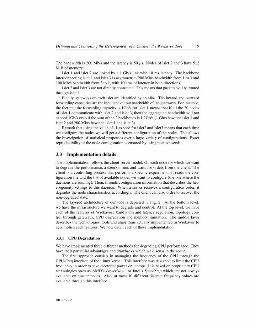
Figure 9: Relative errors. Contribution of each of the timings (CPU, communicationand synchronization.)

for large sizes, when the running time is above 20 seconds, the estimation is veryrealistic with an error margin below 10%.

5.3 Static load balancing

Here, we have benchmarked applications that perform a static load balancing at thebeginning of the application according to the speed of the processors and the amountof work to perform. We have implemented two algorithms that perform parallel matrixmultiplication on heterogeneous environments. The first algorithm from Beaumont et

al. [26] is based on a geometric partition of the columns on the processors. The secondfrom Lastovetsky et al. [27] uses a data partitioning based on a performance model ofthe environment.

We monitored both programs at the MPI level to measure CPU, synchronizationand communication time. We use synchronous send and receive call and timed these

INRIA


calls to measure the communication time. Hence, the communication time is not over-lapped by computation. Moreover, we have added an MPI barrier to synchronize pro-cesses and measure the time each of them spend in the barrier, i.e. neither communi-cating nor computing.

We used 8 of the 11 nodes of the reference platform shown Table 2 (1,4,5,6,7,8,9,10):The other nodes were more powerful than the homogeneous Grid’5000 cluster used forthis experiment and hence it was not possible to emulate them.

Experiments performed on the heterogeneous cluster where highly reproducibleand hence the plot are the average of 3 measures. Concerning the homogeneous clusterwith Wrekavoc plots are the average of 10 measures.

In Fig. 7(a), we show the comparison between the CPU, communication and syn-chronization times for the Beaumont et al. algorithm for matrix sizes of 1000. Nodesare sorted by CPU time. We see that the Wrekavoc behavior is very close to the behav-ior when using the heterogeneous cluster. Also, the proportions of the timings (CPU,communication and synchronization) are preserved. In order to discuss the differencesbetween the two graphs of Fig. 7(a) quantitatively, we plot the relative error in Fig. 9(a).More precisely, in this graph we show the sum of the relative errors of all the timings(CPU, communication and synchronization) of the graphs of Fig. 7(a): for each x valuei and each timing (CPU, communication and synchronization), we compute the rela-tive error 100× abs(ch(i)− cw(i))/Ch(i) where ch(i) (resp., cw(i)) is the value of thetiming for the heterogeneous (resp., Wrekavoc) case for node i and Ch(i) is the sumof the value of the timings on the heterogeneous cluster for node i. In the figure, thedifferent colors then represent the contributions of the three resources.

We see that the overall relative error is always below 10%. The worst case is forprocessor 5 for which the error is mainly due to the synchronization time. In absolutevalues, this timing is very small (less than 0.6 seconds).

In Fig. 7(b), we show the comparison between the CPU, communication and syn-chronization time for the Beaumont et al. algorithm for varying matrix size on a fixednode. We see that the Wrekavoc behavior is very close to the behavior when using theheterogeneous cluster. The only problem concerns an increasing shift of the timingswhen matrix size increases. Indeed, in Fig 9(b), we stack the contribution of the rel-ative error between Wrekavoc and the heterogeneous cluster of all the timings (CPU,communication and synchronization) of the graphs of Fig. 7(b). We see that the overallrelative error is always lower than 10%. Moreover, we see that the contribution of com-munication to the error is marginal (less than 0.6 %). This means that, here, Wrekavocwas able to emulate communication with a great precision.

In Fig. 8(a) and 8(b), we present the same measurements as in Fig. 7(a) and 7(b)but for the Lastovetsky et al. algorithm. Here again, we see that Wrekavoc is veryrealistic with, again, a small shift in execution time when the matrix size increases.In Fig 9(c), we stack the contribution of the relative error between Wrekavoc and theheterogeneous cluster of all the timings (CPU, communication and synchronization) ofthe graphs of Fig. 8(a). From this figure, we can see that the relative error is very lowin general (lower than 6%). There is one exception for processor 5 where the error isa little bit larger than 10%. The relative error of the graphs of Fig. 8(b) are shown inFig. 9(d). Results show that these errors are always lower than 8% and that the CPU

RR n° 7135


20

40

60

80

100

120

0 5 10 15 20 25 30 35 40

Num

ber

of

lines

Interations

load balancing (300*400) Wrekavoc

Proc 1Proc 2Proc 3Proc 4Proc 5Proc 6Proc 7Proc 8

(a) emulation with Wrekavoc

20

40

60

80

100

120

0 5 10 15 20 25 30 35 40

Num

ber

of

lines

Interations

load balancing (300*400) heter. cluster

Proc 1Proc 2Proc 3Proc 4Proc 5Proc 6Proc 7Proc 8

(b) heterogeneous cluster

Figure 10: Comparison of the evolution of the load-balancing for executing the advec-tion diffusion application

and communication times do not contribute a lot to these errors showing that Wrekavocis doing a good job for emulating the heterogeneous hardware.

In conclusion to this section, we see that Wrekavoc precisely emulates the hetero-geneous cluster (within 10%) in the general case. Moreover, most of the relative error iscaused by synchronization. Last, while both algorithms are different and hence providedifferent raw performance, Wrekavoc is able, in both cases, to match their behavior.

5.4 Dynamic load balancing for iterative computation

Here, the dynamic load balancing strategy consists in exchanging some workload atexecution time in function of the progress in the previous iteration. The program wehave used solves an advection-diffusion problem (kinetic chemistry) described in [28].Here, the load corresponds to the number of matrix lines held by each process. At eachiteration to balance the load the nodes send or receive some rows to their neighbours.

As for the previous experiments, we used 8 of the 11 nodes of the reference plat-form shown Table 2 (1,4,5,6,7,8,9,10): The other nodes were more powerful than thehomogeneous cluster we used here and hence it was not possible to emulate them.

In Fig. 10, we show the evolution of the load balancing of this application. At eachiteration, we have monitored the number of matrix rows held by each processor. Weplot the average number of 5 executions during the whole execution of the applicationfor a problem on a surface of 300 columns and 400 matrix rows. There are 40 iterations.The results show that the evolution of the load balancing using Wrekavoc (right) or theheterogeneous cluster (left) are extremely similar. Processor 1 (the fastest), holds anincreasing amount of load in both situation. More interestingly, processor 2 starts offwith a very low load and then its load increases. Moreover, processor 5, the slowestone, is the least loaded at the end.

INRIA


0

2

4

6

8

10

12

14

0 5 10 15 20 25 30 35 40

Rela

tive e

rror

in p

erc

ent

Iterations

Load balancing (300*400). Relative difference between Wrekavoc and Heter. Cluster.

AvgMinMax

Figure 11: Relative error in percent between graphs of Figure 10

In Fig. 11, we show the relative error between the two graphs of Fig. 10. More pre-cisely, for the eight processors involved in these experiments we computed the relativeerror as:

100 × abs(nw(i) − nh(i))/nh(i) for i ∈ [1, 40]

(where nh(i) (resp., nw(i)) is the number of lines treated by a processor of the hetero-geneous cluster (resp., Wrekavoc case) at iteration i. Then, for each iteration, we plotthe maximum, minimum and average value. We see that the error never exceeds 15%on maximum and 7% on average. Moreover the average error relatively stable after30 iterations.

In summary, the predictability of the behavior of the emulated application is veryhigh.

5.5 The master-worker paradigm

The next set of experiments concerns the master-worker paradigm. We have a masterthat holds some data and a set of workers that are able to process the data. When aworker is idle, it asks the master for some data to process, performs the computationand sends the results back. Such paradigm allows for a dynamic load balancing. Asan application of this paradigm, we have chosen parallel image rendering with the

RR n° 7135


0

5

10

15

20

25

30

1200 * 1200 1200 * 1000 1000 * 1000 1000 * 800 800 * 800 800 * 600 600 * 600 600 * 400

Execution t

ime (

in s

econds)

Image size

constant 100*100 block size

Heter. ClusterWrekavoc

(a) block size of 100 × 100 and different image sizes

0

10

20

30

40

50

50 * 50 100 * 50 100 * 100 200 * 100 200 * 200 400 * 200 400 * 400

Execution t

ime (

in s

econds)

Block size

Fixed image size: 1000 * 800


(b) image size 1000 × 800 with different block sizes

Figure 12: Parallel rendering times of the master-worker application

INRIA


Povray [29] ray-tracer. Here, the master holds a synthetic description of a scene. Thisscene is decomposed into blocks such that each part can be processed by a worker.

We used 6 of the 11 nodes of the reference platform shown Table 2 (1,2,4,5,6,7):node 3 is equivalent to node 2 and hence was not used, node 8 and 9 had performancetoo close to node 7, node 10 was not powerful enough fort Povray and node 11 was toopowerful to be emulated on the homogeneous Grid’5000 cluster.

In Fig. 12(a) (resp., 12(b)), we present the comparison between the running timeof the application when the block size is fixed (resp., the image size is fixed) and theimage size varies (resp., the block size varies). Each plot is the average of 5 runs.

We see that, most of the time, Wrekavoc is able to match reality, at least quantita-tively. Indeed, if we order the block-size by running time the Wrekavoc order is thesame than the heterogeneous cluster order.

5.6 The work stealing paradigm

Here, we benchmark the behavior of different work-stealing algorithms. Within thisparadigm, an underloaded node chooses another node to ask for some work. Our cho-sen application for this methodology is the N -queen problem. This problem consistsin placing N queens on a check board of size N × N , such that no queen is blockedby any other one. The goal of the application is to find all the possible solutions for agiven N . To solve this problem, we place M queens on the top M rows and generate,for each possible placement (there exists NM such placement), a sub-problem that hasto be processed sequentially. This problem is irregular: two sub-problem restricted tothe same number of rows can have very different number of solutions and may requirevery different running times.

When a node is underloaded, different strategies can be applied to choose the nodewhere work is stolen.

Algo1: c1 d1 g1 (random load stealing,load evenly distributed, granularity 14)Algo2: c2 d1 g2 Algo3: c1 d2 g2Algo4: c1 d3 g2 Algo5: c1 d4 g2Algo6: c1 d5 g2 Algo7: c1 d1 g5Algo8: c1 d1 g3 Algo9: c1 d1 g1

Strategy c1: choose node at random; c2: chose one of two designated neighbors (nodesare arranged according to a virtual ring). The way the load is distributed initially mayalso have an impact. Here, we use 5 different strategies. Distribution d1: The loadis evenly distributed; d2: Place all the load on the fastest node; d3: Place all the loadon the slowest node; d4: Place all the load on an average speed node; d5: Place allthe load on the second slowest node. When solving the N -queen problem, the load iscomposed of tasks that have a given granularity (i.e., M , the number queens alreadyplaced). We fixed N = 17 and studied different granularities. Granularity g1: 2 rows;g2: 3 rows; g3: 4 rows; g4: 5 rows.

RR n° 7135


With these different characteristics, we have chosen 9 different algorithms out ofthe 50 possible combinations.3 These 9 algorithms are depicted in the above table.

0

500

1000

1500

2000

2500

3000

3500

Algo 1 Algo 2 Algo 3 Algo 4 Algo 5 Algo 6 Algo 7 Algo 8 Algo 9

Execution t

ime (

in s

econds)

Algorithm

N-queen 17 mono-threaded


Figure 13: Computation time of the different algorithms for the N -queen problem ofsize 17, using the heterogeneous cluster or Wrekavoc, kernel 2.6.18

We used 8 of the 11 nodes of the reference platform shown Table 2 (1,4,5,6,7,8,9,10):The other nodes were more powerful than the homogeneous Grid’5000 cluster used forthis experiment and hence it was not possible to emulate them.

The results are average timing of 6 runs. In Fig. 13, we present the results for thesingle-threaded implementation of the 9 algorithms. We see that Wrekavoc is able toreproduce the behavior of the heterogeneous cluster precisely. Timings are almost thesame in both situations.

We have implemented a multi-threaded version of the algorithm; one thread for thecomputation and one thread for the communication. We have benchmarked Wrekavocwith two kernel versions 2.6.18 and 2.6.23. The difference between these two versionsis a change in the process scheduler. The 2.6.18 version uses the O(1) scheduler, whilethe 2.6.23 version of the kernel implements the so-called Completely Fair Scheduling

(CFS), based on fair queuing [31]. Both schedulers are kernel developments of IngoMolnar from Redhat Corp.

We present the results for both kernel versions in Fig. 14. We first see that the multi-threaded version is faster than the single-threaded (especially when the load is initiallyplaced on slow processors (Algorithms 4, 5 and 6)). We see that Wrekavoc is ableto reproduce this acceleration from the single threaded version to the multi-threaded.Moreover, we see that using kernel 2.6.23 improves the accuracy of Wrekavoc whenexperimenting a multi-threaded program. This holds especially for algorithms usingthe g2 granularity (algorithms 1 to 6). A higher granularity reduces the realism because

3We favored Strategy c1 since it is known to be the best for this application [30]

INRIA


0

500

1000

1500

2000

2500

3000


Execution t

ime (

in s

econds)

Algorithm

N-queen 17 multi-threaded (2.6.18)


(a) With kernel 2.6.18

0

500

1000

1500

2000

2500

3000


Execution t

ime (

in s

econds)

Algorithm

N-queen 17 multi-threaded (2.6.23)


(b) With kernel 2.6.23

Figure 14: Computation time of the different algorithms for the N -queen problem ofsize 17, using the heterogeneous cluster or Wrekavoc, multi-threaded version, kernel2.6.18 and 2.6.23

RR n° 7135


the number of tasks to execute lowers when the granularity increases and hence makesit difficult to reproduce the behavior.

We explain the fact that the realism of Wrekavoc is better with kernel 2.6.23 thanwith kernel 2.6.18 by the difference of the process scheduler implemented in this twoversions. In Unix processes are scheduled according to their priority. This prioritychanges with the behavior of the process. The problem for the O(1) scheduling algo-rithm of kernel 2.6.18 is that Wrekavoc adds a bias in the way the process priority iscomputed by stopping and continuing process on for its own purpose. Indeed, the O(1)scheduler tends to favor I/O restricted processes. When Wrekavoc suspends a processfor controlling the CPU speed and wakes it up later, the scheduler increases the processpriority (taking it for a I/O bound process). Therefore, both threads (communicationand CPU) of the process have acquired the same priority whereas the communicationthread should have a higher priority: the process does not spend enough time in com-munication. Therefore, the behavior is extremely unrealistic when all the load is ona slow processor at the beginning. The CFS scheduling algorithm (of kernel 2.6.23)solves this problem giving extra priority to suspended processes similar to those thathad been scheduled off when waiting for I/O. In conclusion, this shows that emulationof multi-threaded programs is realistic if running Wrekavoc on a recent Linux kernelversion (at least 2.6.23).

6 Scalability

In the previous section, we could not use more than 12 processors because it was notpossible to have a larger heterogeneous reference cluster under satisfying experimentalconditions. Nevertheless, we want to evaluate the scalability of Wrekavoc on a largesetting using hundreds of nodes. Since there is no real execution to compare it with,we will only be able to analyze the behavior on the environment heterogeneized byWrekavoc.

6.1 CPU intensive benchmarks

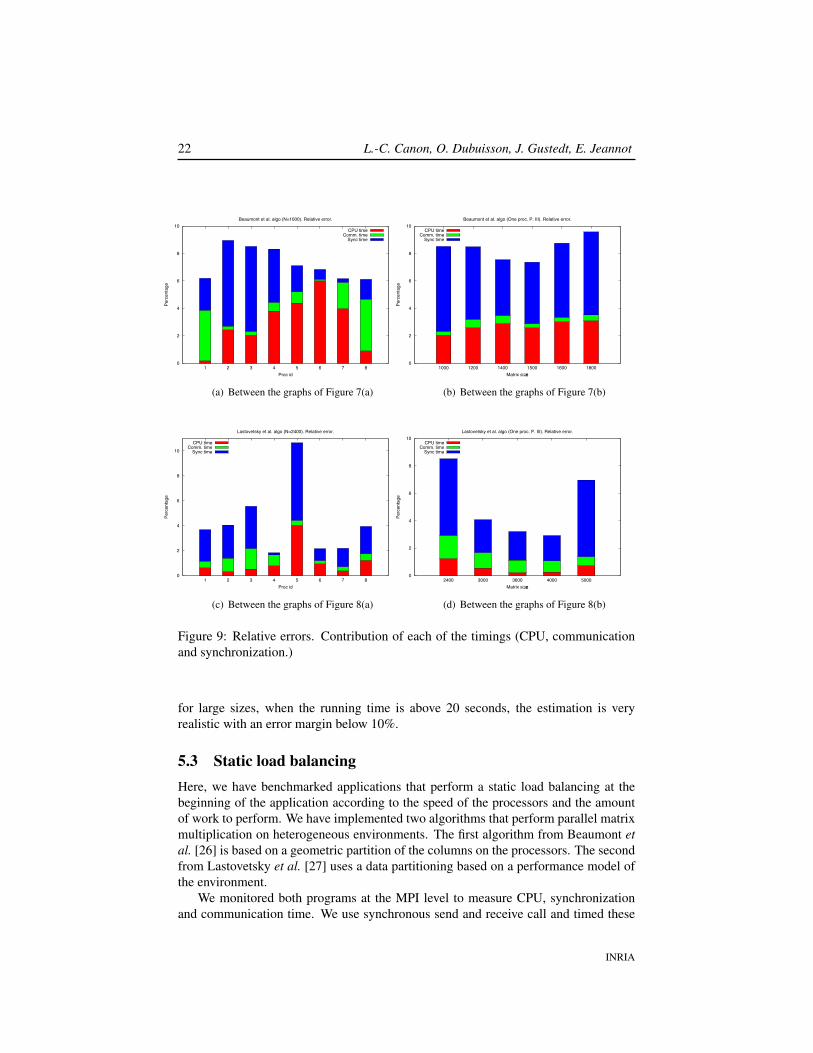
Here, we use the Lastovetsky et al. matrix multiplication algorithm for heterogeneousenvironment. As in the previous experiment, we used the Grelon Cluster of the NancyGrid’5000 site.

We have used different configurations. Each configuration is made of 8 islets. Eachislet has one gateway to communicate with the other 7 islets. We have two settings ofCPU speeds and two settings of network regulation. Concerning CPU speeds we have:

• Fast CPU speeds: all nodes of islet 1: 1550 MHz, islet 2: 1400 MHz, . . . islet 8:500 MHz.

• Slow CPU speeds: all nodes of islet 1: 775 MHz, islet 2: 700 MHz, . . . islet 8:250 MHz.

Concerning Network speed, we have:

INRIA


• Fast Net speeds A clique at 1Gb/s and min latency (the latency of the underlyingcluster without degradation).

• Slow Net speeds A clique at 100 Mb/s and 0.05 ms latency.

By combining network and CPU speeds, we obtain 4 different settings. For eachsetting, we use a different number of nodes per islet (from 1 to 13) leading to configu-ration having between 8 to 104 nodes.

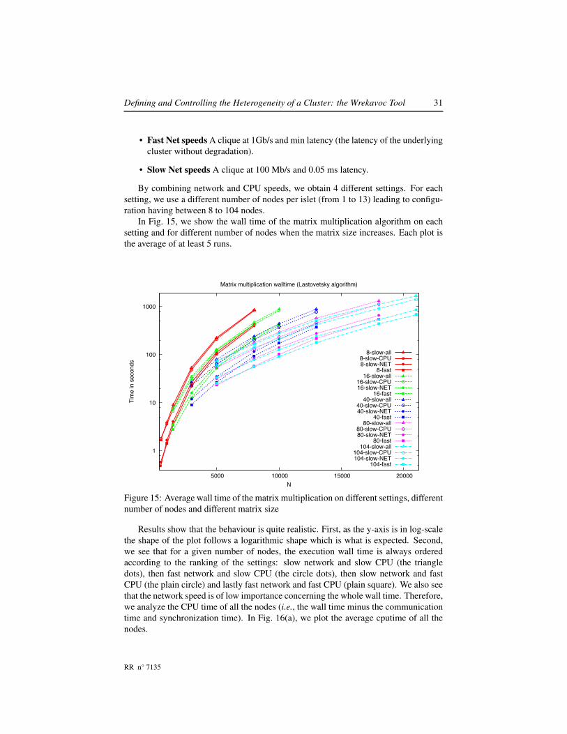
In Fig. 15, we show the wall time of the matrix multiplication algorithm on eachsetting and for different number of nodes when the matrix size increases. Each plot isthe average of at least 5 runs.

1

10

100

1000

5000 10000 15000 20000

Tim

e in s

econds

N

Matrix multiplication walltime (Lastovetsky algorithm)

8-slow-all8-slow-CPU8-slow-NET

8-fast16-slow-all

16-slow-CPU16-slow-NET

16-fast40-slow-all


40-fast80-slow-all


80-fast104-slow-all


104-fast

Figure 15: Average wall time of the matrix multiplication on different settings, differentnumber of nodes and different matrix size

Results show that the behaviour is quite realistic. First, as the y-axis is in log-scalethe shape of the plot follows a logarithmic shape which is what is expected. Second,we see that for a given number of nodes, the execution wall time is always orderedaccording to the ranking of the settings: slow network and slow CPU (the triangledots), then fast network and slow CPU (the circle dots), then slow network and fastCPU (the plain circle) and lastly fast network and fast CPU (plain square). We also seethat the network speed is of low importance concerning the whole wall time. Therefore,we analyze the CPU time of all the nodes (i.e., the wall time minus the communicationtime and synchronization time). In Fig. 16(a), we plot the average cputime of all thenodes.

RR n° 7135


0.1

1

10

100

1000

5000 10000 15000 20000

Tim

e in s

econds

N

Matrix multiplication average CPU time (Lastovetsky algorithm)

8-fast8-slow16-fast

16-slow40-fast

40-slow80-fast

80-slow104-fast

104-slow32-slow

(a) CPU time

0.85

0.9

0.95

1

1.05

1.1

2000 4000 6000 8000 10000 12000 14000 16000 18000

Norm

aliz

ed t

ime (

t*p/N

3)

N

Matrix multiplication normalized CPU time (Lastovetsky algorithm)

8-fast8-slow16-fast

16-slow40-fast

40-slow80-fast

80-slow104-fast

104-slow

(b) Normalized CPU time

Figure 16: Average cputime and normalized of the matrix multiplication on differentsettings different number of nodes and different matrix size

INRIA


N Receivers

GW1 GW2

X Mb/s

Y Mb/s

X Mb/s

N Senders(a) Redistribution pattern

1 Receiver

GW1 GW2Y Mb/s

N Senders

X1 Mb/s

X2 Mb/s

(b) Gather pattern

Figure 17: Communication pattern for benchmarking gateway scalability. X is thebandwidth of the intra-islet communication and Y of the bandwidth of the inter-isletcommunication

We observe another very interesting property. When we use a fast setting (cross)with a given number of nodes, the emulated CPU time is exactly the same with twiceas much processors but for a slow setting (circle dots). This is exactly what we wouldexpect with a perfect load balancing: islets in the fast setting are made of nodes thatare twice as fast than in the slow setting. This shows that the Lastovetsky algorithm isable to perform a very good load balancing and that Wrekavoc emulates the CPU speedwith a great precision. This also indicates that it is possible to normalize all the CPUtime according to the number of nodes, the CPU setting, and a given reference point.Actually, based on the fact that the number of operations of a matrix multiplication isN3 where N is the order of the matrix, we have the following normalizing formula:

t × p × f

N3

where t is the running time, p is the number of used processors and f equals 1 slowCPU setting and 2 for fast CPU setting.

In Fig. 16(b), we plot the normalized cputime according to the above formula. Wehave further normalized the plot such that the slow setting with 16 nodes and N =2000 point has a value of 1. Based on that figure we see that all the points are within10 percent of the expected value. The only exception is for slow setting, 8 nodes,N = 5000 for which the error is 13%. This is due to the fact that for that particularsetting, the process durations are very small (in the order of 10 ms).

6.2 Scalability of gateways

In order to benchmark the gateways and their scalability, we have set two configura-tions. Such configurations lead to an overlay network whose topology is depicted inFig. 17(a) for a redistribution pattern and Fig. 17(b) for a gather pattern.

To perform the benchmark we used the GDX Cluster of the Orsay Grid’5000 site.These benchmarks consists in measuring the bandwidth that is observed for networkstreams between two nodes of different islets. The expected behavior is that the aggre-gated bandwidth should increase linearly until it reaches the bandwidth of the inter-isletlink. Beyond that point, the inter-islet bandwidth is shared between the different com-

RR n° 7135


4

6

10

20

50

100

200

500

1 2 5 10 20 50 100

4

6

10

20

50

100

200

500

Bandw

idth

(M

bit/s

)

Number of streams

Backbone 500 - node 10

cumulated BWMin BWAvg BW

(a) Backbone: 500 Mb/s; inter-islet: 10 Mb/s

1

4

6

10

20

50

100

1 2 5 10 20 50 100

1

4

6

10

20

50

100

Bandw

idth

(M

bit/s

)

Number of streams

Backbone 100 - node 20


(b) Backbone: 100 Mb/s; inter-islet: 20 Mb/s

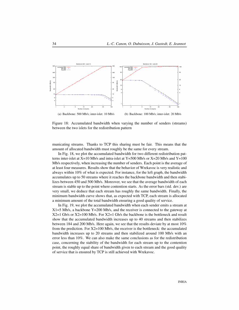
Figure 18: Accumulated bandwidth when varying the number of senders (streams)between the two islets for the redistribution pattern

municating streams. Thanks to TCP this sharing must be fair. This means that theamount of allocated bandwidth must roughly be the same for every stream.

In Fig. 18, we plot the accumulated bandwidth for two different redistribution pat-terns inter-islet at X=10 Mb/s and intra-islet at Y=500 Mb/s or X=20 Mb/s and Y=100Mb/s respectively, when increasing the number of senders. Each point is the average ofat least four measures. Results show that the behavior of Wrekavoc is very realistic andalways within 10% of what is expected. For instance, for the left graph, the bandwidthaccumulates up to 50 streams where it reaches the backbone bandwidth and then stabi-lizes between 450 and 500 Mb/s. Moreover, we see that the average bandwidth of eachstream is stable up to the point where contention starts. As the error bars (std. dev.) arevery small, we deduce that each stream has roughly the same bandwidth. Finally, theminimum bandwidth curve shows that, as expected with TCP, each stream is allocateda minimum amount of the total bandwidth ensuring a good quality of service.

In Fig. 19, we plot the accumulated bandwidth when each sender emits a stream atX1=5 Mb/s, a backbone Y=200 Mb/s, and the receiver is connected to the gateway atX2=1 Gb/s or X2=100 Mb/s. For X2=1 Gb/s the backbone is the bottleneck and resultshow that the accumulated bandwidth increases up to 40 streams and then stabilizesbetween 184 and 200 Mb/s. Here again, we see that the results deviate by at most 10%from the prediction. For X2=100 Mb/s, the receiver is the bottleneck: the accumulatedbandwidth increases up to 20 streams and then stabilized around 100 Mb/s with anerror less than 10%. We can also make the same conclusions as for the redistributioncase, concerning the stability of the bandwidth for each stream up to the contentionpoint, the roughly equal share of bandwidth given to each stream and the good qualityof service that is ensured by TCP is still achieved with Wrekavoc.

INRIA


1

2

5

10

20

50

100

200

1 2 4 10 20 40 100 200

1

2

5

10

20

50

100

200

Bandw

idth

(M

bit/s

)

Number of streams

Gather n to 1. Backbone 200, links n*5, link 1000


(a) X1=5 Mb/s, Y=200 Mb/s and X2=1 Gb/s

1

2

5

10

20

50

100

1 2 4 10 20 40 100

1

2

5

10

20

50

100

Bandw

idth

(M

bit/s

)

Number of streams

Gather n to 1. Backbone 200, links n*5, link 100


(b) X1=5 Mb/s, Y=200 Mb/s and X2=100 Mb/s

Figure 19: Accumulated bandwidth when varying the number of senders (streams)between the two islets for the gather pattern

7 Conclusion and Future Work

Nowadays computing environments are more and more complex. Analytic validationof solutions for these environments are not always possible or not always sufficient.

In this work, we propose a new approach called Wrekavoc for emulating heteroge-neous distributed computing platforms that are based upon the Linux kernel. Wrekavocdefines and controls the heterogeneity of a given platform by degrading CPU, by reg-ulating the network or by limiting the memory of each node and by composing theemulated platform as a static overlay. The overall goal is to provide an environment onwhich reproducible experiments on heterogeneous settings are eased.

Our current implementation of Wrekavoc has been tested, benchmarked and evalu-ated in several ways. First, we have shown that configuring a set of nodes is very fast.Micro-benchmarks show that we are able to independently degrade CPU, bandwidthand latency to the desired values.

Second, we have validated Wrekavoc by comparing the execution of several real ap-plications on a real environments to a reference cluster running Wrekavoc. The resultsobtained in the experiments concern all the features of Wrekavoc (network regulation,memory limitation and CPU degradation). Wrekavoc is realistic and has a very goodreproducibility. Moreover, the tool provides emulations that are not tied to the real hostplatform: at the application/user level, different architectural features (e.g., processorarchitecture, memory bandwidth, cache, instruction sets, etc.) are correctly emulated.

Last, we have performed a set of experiments to assess the scalability of Wrekavoc.Concerning scalability at the CPU level we have performed benchmarks using morethan 100 nodes and for those concerning the network up to 200 nodes. In both cases,we see that the behaviour is very close to what is expected.

All these results show that Wrekavoc is a suitable tool for developing, studying andcomparing algorithms in heterogeneous environments: in almost all cases results are

RR n° 7135


within 10% of what is expected (from theory or other real benchmarks). The realism iseven better when the runtime of the program under investigation or the communicationtime is long enough (1s or more).

Future work are directed to the improvement of the realism of Wrekavoc for low-level features such as cache, memory bandwidth or disk IO. Moreover, it seemed im-portant to us to first be able to emulate static heterogeneous platforms accurately. In asecond step, we now hope to be able to emulate dynamic features. Hence, future workwill be directed towards the ease of the calibration of the environment, a better emula-tion of multi-threaded programs and to new modeling features such as node volatilityand dynamic load.

Acknowledgment

This work was supported by a one year internship grant for the second author byFONGECIF to INRIA Nancy – Grand Est.

Experiments presented in this paper were carried out using the Grid’5000 experi-mental testbed, being developed under the INRIA ALADDIN development action withsupport from CNRS, RENATER and several Universities as well as other funding bod-ies (see https://www.grid5000.fr).

References

[1] I. Foster, C. Kesselman, The Grid: Blueprint for a New Computing Infrastructure,Morgan-Kaufmann, 1998.

[2] The Grid’5000 experimental testbed.URL https://www.grid5000.fr

[3] I. Stoica, R. Morris, D. Karger, M. F. Kaashoek, H. Balakrishnan, Chord: Ascalable peer-to-peer lookup service for internet applications, in: SIGCOMM ’01:Proceedings of the 2001 conference on Applications, technologies, architectures,and protocols for computer communications, ACM, New York, NY, USA, 2001,pp. 149–160. doi:http://doi.acm.org/10.1145/383059.383071.

[4] A. Oram (Ed.), Peer-to-Peer: Harnessing the Power of Disruptive Technologies,O’Reilly & Associates, Inc., Sebastopol, CA, USA, 2001.

[5] D. P. Anderson, Boinc: A system for public-resource computing and storage, in:GRID ’04: Proceedings of the 5th IEEE/ACM International Workshop on GridComputing, IEEE Computer Society, Washington, DC, USA, 2004, pp. 4–10.doi:http://dx.doi.org/10.1109/GRID.2004.14.

[6] G. Fedak, C. Germain, V. Neri, F. Cappello, Xtremweb: A generic global com-puting system, in: CCGRID, IEEE Computer Society, Los Alamitos, CA, USA,2001, pp. 582–587.

INRIA

https://www.grid5000.fr



http://dx.doi.org/http://doi.acm.org/10.1145/383059.383071

http://dx.doi.org/http://dx.doi.org/10.1109/GRID.2004.14


[7] J. Gustedt, E. Jeannot, M. Quinson, Experimental Methodologies for Large-ScaleSystems: a Survey, Parallel Processing Letters 19 (3) (2009) 399–418.

[8] H. Casanova, A. Legrand, M. Quinson, SimGrid: a Generic Framework for Large-Scale Distributed Experiments, in: 10th IEEE International Conference on Com-puter Modeling and Simulation, 2008.

[9] R. Buyya, M. M. Murshed, GridSim: A toolkit for the modeling and simulationof distributed resource management and scheduling for grid computing, Journalof Concurrency and Computation: Practice and Experience 14 (13–15).

[10] H. Xia, H. Dail, H. Casanova, A. A. Chien, The microgrid: Using online simula-tion to predict application performance in diverse grid network environments, in:Challenges of Large Applications in Distributed Environments (CLADE), Hon-olulu, HI, USA, 2004, p. 52.

[11] A. Vahdat, K. Yocum, K. Walsh, P. Mahadevan, D. Kostic, J. Chase, D. Becker,Scalability and accuracy in a large-scale network emulator, SIGOPS Oper. Syst.Rev. 36 (SI) (2002) 271–284. doi:http://doi.acm.org/10.1145/

844128.844154.

[12] Grid explorer (GdX).URL http://www.lri.fr/˜fci/GdX/

[13] The DAS-3 project.URL http://www.cs.vu.nl/das3/

[14] Planet lab.URL http://www.planet-lab.org/

[15] A. Takefusa, S. Matsuoka, H. Nakada, K. Aida, U. Nagashima, Overview of a per-formance evaluation system for global computing scheduling algorithms, in: the8th IEEE International Symposium on High Performance Distributed Computing(HPDC’99), Redondo Beach, California, USA, 1999.

[16] H. Lamehamedi, Z. Shentu, B. Szymanskia, E. Deelman, Simulation of dynamicdata replication strategies in data grids, in: the 17th International Symposium onParallel and Distributed Processing, Nice, France, 2003, pp. 10pp+.

[17] H. Lamehamedi, B. Szymanski, Z. Shentu, , E. Deelman, Data replication strate-gies in grid environments, in: Proc. Of the Fifth International Conference onAlgorithms and Architectures for Parallel Processing, 2002, pp. 378–383.

[18] The network simulator NS2.URL http://www.isi.edu/nsnam/ns

[19] J. Prokkola, Opnet - network simulator (2007).URL http://www.telecomlab.oulu.fi/kurssit/521365A_

tietoliikennetekniikan_simuloinnit_ja_tyokalut/Opnet_

esittely_07.pdf

RR n° 7135



http://www.lri.fr/~fci/GdX/

http://www.lri.fr/~fci/GdX/

http://www.cs.vu.nl/das3/

http://www.cs.vu.nl/das3/

http://www.planet-lab.org/

http://www.planet-lab.org/

http://www.isi.edu/nsnam/ns

http://www.isi.edu/nsnam/ns

http://www.telecomlab.oulu.fi/kurssit/521365A_tietoliikennetekniikan_simuloinnit_ja_tyokalut/Opnet_esittely_07.pdf





[20] A. Varga, The omnet++ discrete event simulation system (2001).URL http://www.omnetpp.org/download/docs/papers/

esm2001-meth48.pdf

[21] P. Vicat-Blanc Primet, O. Gluck, C. Otal, F. Echantillac, Emulation d’un nuagereseau de grilles de calcul: eWAN, Tech. Rep. RR 2004-59, LIP ENS, Lyon,France (2004).

[22] The RAMP project: Research Accelerator for Multiple Processors.URL http://ramp.eecs.berkeley.edu/

[23] iproute2+tc notes: http://snafu.freedom.org/linux2.2/

iproute-notes.html.

[24] parXXL: A fine grained development environment on coarse grained architec-tures.URL http://parxxl.gforge.inria.fr/

[25] A. V. Gerbessiotis, L. G. Valiant, Direct bulk-synchronous parallel algorithms,Journal of Parallel and Distributed Computing 22 (1994) 251–267.

[26] O. Beaumont, V. Boudet, F. Rastello, Y. Robert, Matrix multiplication on het-erogeneous platforms, IEEE Trans. Parallel Distributed Systems 12 (10) (2001)1033–1051.

[27] A. Lastovetsky, R. Reddy, Data partitioning with a realistic performance modelof networks of heterogeneous computers with task size limits, in: Proceedings ofthe Third International Symposium on Parallel and Distributed Computing / ThirdInternational Workshop on Algorithms, Models and Tools for Parallel Comput-ing on Heterogeneous Networks (ISPDC/HeteroPar‘04), IEEE Computer SocietyPress, 2004, pp. 133–140.

[28] F. Vernier, Algorithmique iterative pour l’equilibrage de charge dans les reseauxdynamiques, Ph.D. thesis, Univ. de Franche-Comte (2004).

[29] The persistence of vision raytracer.URL http://www.povray.org/

[30] R. D. Blumofe, C. E. Leiserson, Scheduling multithreaded computations by workstealing, J. ACM 46 (5) (1999) 720–748. doi:http://doi.acm.org/10.1145/324133.324234.

[31] J. Nagle, On packet switches with infinite storage, IETF RFC 970 (1985).URL http://www.rfc-archive.org/getrfc.php?rfc=970

INRIA

http://www.omnetpp.org/download/docs/papers/esm2001-meth48.pdf



http://ramp.eecs.berkeley.edu/

http://ramp.eecs.berkeley.edu/

http://snafu.freedom.org/linux2.2/iproute-notes.html

http://snafu.freedom.org/linux2.2/iproute-notes.html

http://parxxl.gforge.inria.fr/



http://www.povray.org/

http://www.povray.org/



http://www.rfc-archive.org/getrfc.php?rfc=970

http://www.rfc-archive.org/getrfc.php?rfc=970

Centre de recherche INRIA Nancy – Grand EstLORIA, Technopôle de Nancy-Brabois - Campus scientifique

615, rue du Jardin Botanique - BP 101 - 54602 Villers-lès-Nancy Cedex (France)

Centre de recherche INRIA Bordeaux – Sud Ouest : Domaine Universitaire - 351, cours de la Libération - 33405 Talence CedexCentre de recherche INRIA Grenoble – Rhône-Alpes : 655, avenue de l’Europe - 38334 Montbonnot Saint-Ismier

Centre de recherche INRIA Lille – Nord Europe : Parc Scientifique de la Haute Borne - 40, avenue Halley - 59650 Villeneuve d’AscqCentre de recherche INRIA Paris – Rocquencourt : Domaine de Voluceau - Rocquencourt - BP 105 - 78153 Le Chesnay CedexCentre de recherche INRIA Rennes – Bretagne Atlantique : IRISA, Campus universitaire de Beaulieu - 35042 Rennes Cedex

Centre de recherche INRIA Saclay – Île-de-France : Parc Orsay Université - ZAC des Vignes : 4, rue Jacques Monod - 91893 Orsay CedexCentre de recherche INRIA Sophia Antipolis – Méditerranée : 2004, route des Lucioles - BP 93 - 06902 Sophia Antipolis Cedex

ÉditeurINRIA - Domaine de Voluceau - Rocquencourt, BP 105 - 78153 Le Chesnay Cedex (France)

http://www.inria.fr

ISSN 0249-6399

Defining and Controlling the Heterogeneity of a … · Defining and Controlling the Heterogeneity...

Documents

Transcript of Defining and Controlling the Heterogeneity of a … · Defining and Controlling the Heterogeneity...