
Defense Talk Slides
141
Estimating phylogenetic trees from discrete morphological data Thesis Defense April M. Wright April 14, 2015 Supervising Professor: David M. Hillis 1
-
Upload
april-wright -
Category
Science
-
view
435 -
download
0
Transcript of Defense Talk Slides
Estimating phylogenetic trees from discrete morphological data
Thesis DefenseApril M. WrightApril 14, 2015
Supervising Professor: David M. Hillis1
2
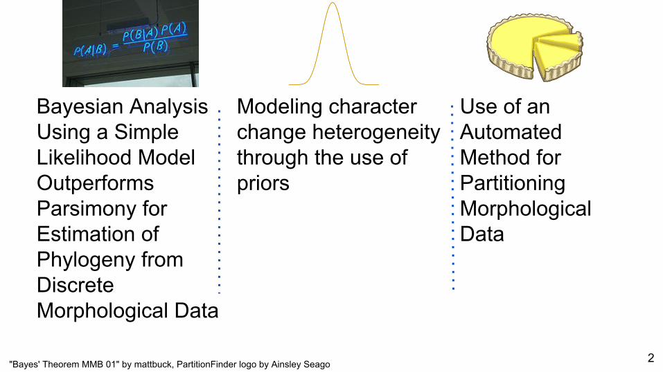
Bayesian Analysis Using a Simple Likelihood Model Outperforms Parsimony for Estimation of Phylogeny from Discrete Morphological Data
Modeling character change heterogeneity through the use of priors
Use of an Automated Method for Partitioning Morphological Data
"Bayes' Theorem MMB 01" by mattbuck, PartitionFinder logo by Ainsley Seago

Why Morphology?
3
Why Morphology?● Estimates put > 99% of biota that has ever existed as extinct
4
Why Morphology?● Estimates put > 99% of biota that has ever existed as extinct● Probably, we won’t wring DNA from a stone
5
Why Morphology?● Estimates put > 99% of biota that has ever existed as extinct● Probably, we won’t wring DNA from a stone● Inclusion of fossils acknowledged to improve phylogenetic trees
(Huelsenbeck 1991, Wiens 2001 & 2004), divergence dating (Heath, Stadler and Huelsenbeck
2012) and comparative method estimates (Slater and Harmon 2012)
6
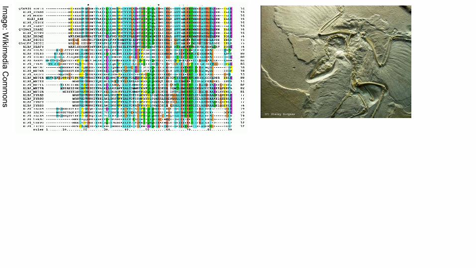
Image: W
ikimedia C
omm
ons
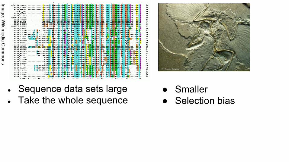
Image: W
ikimedia C
omm
ons
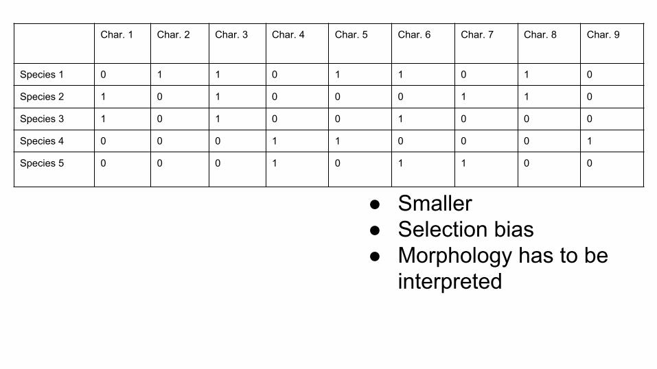
● Smaller● Selection bias
● Sequence data sets large● Take the whole sequence
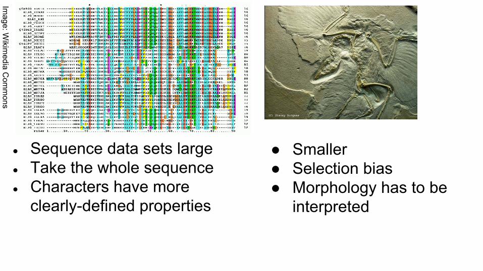
Image: W
ikimedia C
omm
ons
● Smaller● Selection bias● Morphology has to be
interpreted
● Sequence data sets large● Take the whole sequence● Characters have more
clearly-defined properties
● Smaller● Selection bias● Morphology has to be
interpreted
Char. 1 Char. 2 Char. 3 Char. 4 Char. 5 Char. 6 Char. 7 Char. 8 Char. 9
Species 1 0 1 1 0 1 1 0 1 0
Species 2 1 0 1 0 0 0 1 1 0
Species 3 1 0 1 0 0 1 0 0 0
Species 4 0 0 0 1 1 0 0 0 1
Species 5 0 0 0 1 0 1 1 0 0
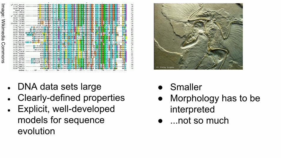
Image: W
ikimedia C
omm
ons
● Smaller● Morphology has to be
interpreted ● ...not so much
● DNA data sets large● Clearly-defined properties● Explicit, well-developed
models for sequence evolution
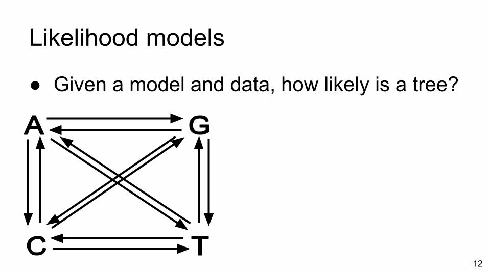
Likelihood models
● Given a model and data, how likely is a tree?
12
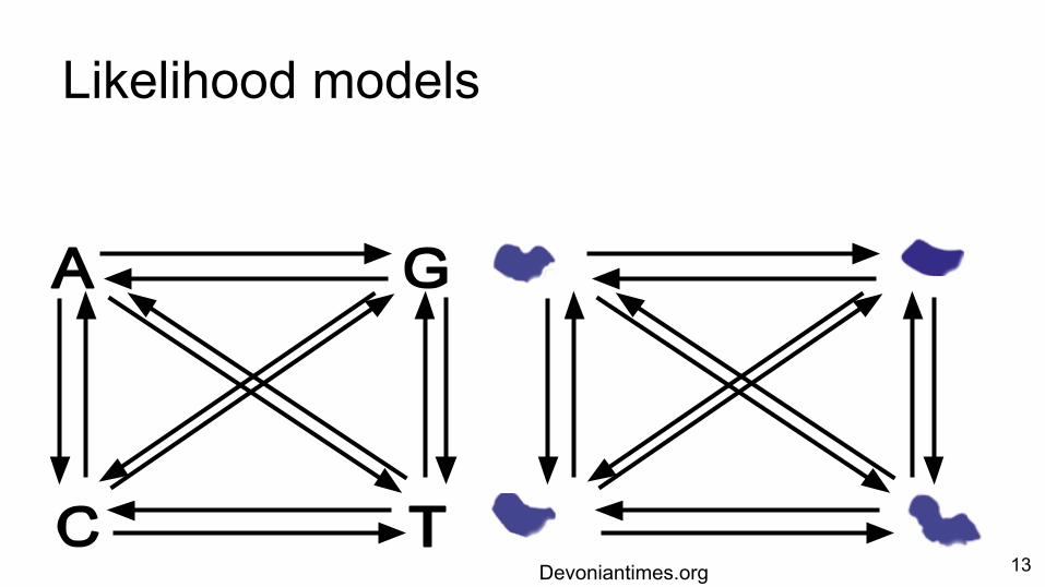
Likelihood models
● Given a model and data, how likely is a tree?
Devoniantimes.org 13
Chapter One: Bayesian Analysis Using a Simple Likelihood Model Outperforms Parsimony for Estimation of Phylogeny from Discrete Morphological Data
14
Likelihood models
● There is one practical published model for phylogenetic estimation from discrete morphological data, Mk
15
Likelihood models
● There is one practical published model for phylogenetic estimation from discrete morphological data, Mk○ Like all methods, Mk has assumptions
16
Likelihood models
● There is one practical published model for phylogenetic estimation from discrete morphological data, Mk○ Like all methods, Mk has assumptions
■ Change can occur at any instant along a branch■ Change is symmetrical between states
17
Likelihood models
● There is one practical published model for phylogenetic estimation from discrete morphological data, Mk○ Like all methods, Mk has assumptions
■ Change can occur at any instant along a branch■ Change is symmetrical between states
● This model is statistically consistent
18
Likelihood models
● There is one practical published model for phylogenetic estimation from discrete morphological data, Mk○ Like all methods, Mk has assumptions
■ Change can occur at any instant along a branch■ Change is symmetrical between states
● This model is statistically consistent○ Caveat: As long as the assumptions hold○ Also, we don't have infinite data 19
Does a parametric approach (Mk) outperform non-parametric approach
(parsimony) when model assumptions are violated?
20
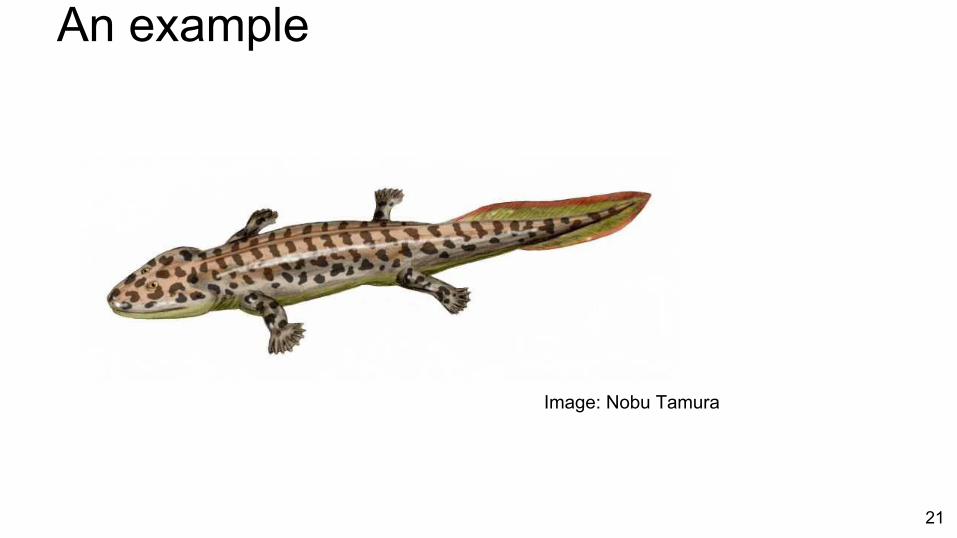
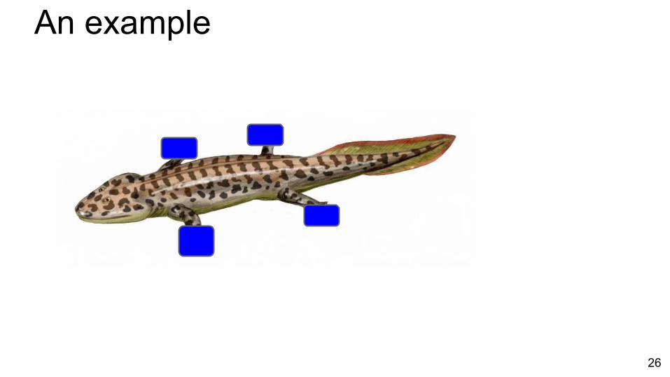
An example
Image: Nobu Tamura
21
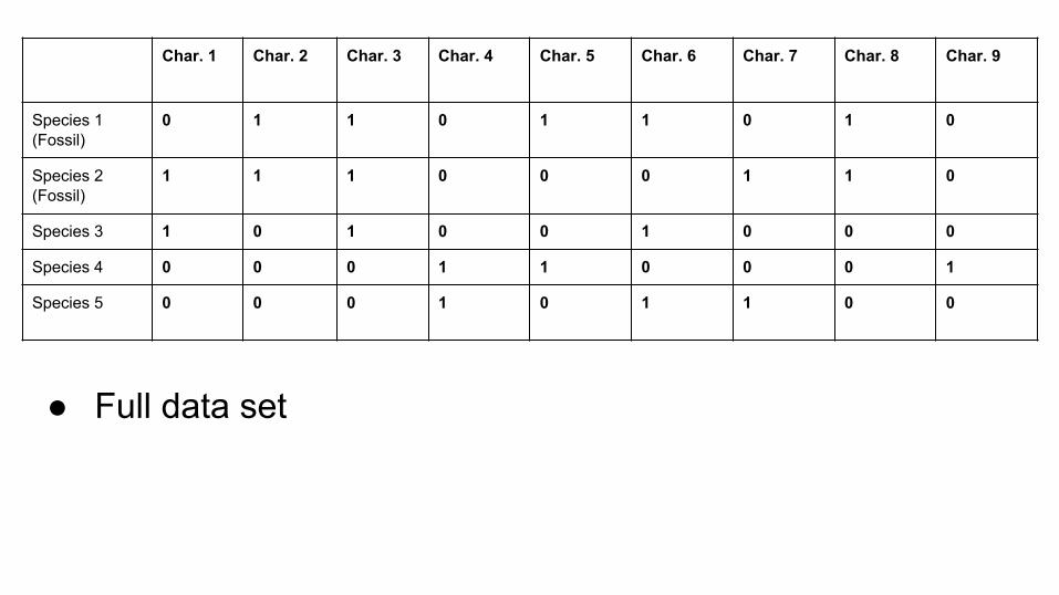
● Full data set
Char. 1 Char. 2 Char. 3 Char. 4 Char. 5 Char. 6 Char. 7 Char. 8 Char. 9
Species 1(Fossil)
0 1 1 0 1 1 0 1 0
Species 2(Fossil)
1 1 1 0 0 0 1 1 0
Species 3 1 0 1 0 0 1 0 0 0
Species 4 0 0 0 1 1 0 0 0 1
Species 5 0 0 0 1 0 1 1 0 0
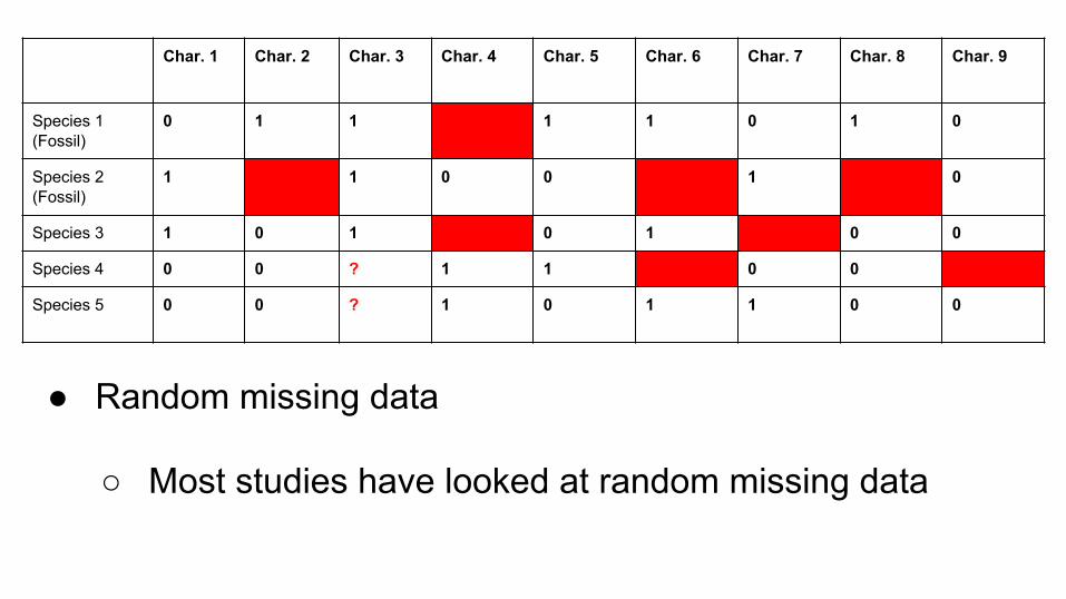
● Random missing data
○ Most studies have looked at random missing data
Char. 1 Char. 2 Char. 3 Char. 4 Char. 5 Char. 6 Char. 7 Char. 8 Char. 9
Species 1(Fossil)
0 1 1 ? 1 1 0 1 0
Species 2(Fossil)
1 ? 1 0 0 ? 1 ? 0
Species 3 1 0 1 ? 0 1 ? 0 0
Species 4 0 0 ? 1 1 ? 0 0 ?
Species 5 0 0 ? 1 0 1 1 0 0
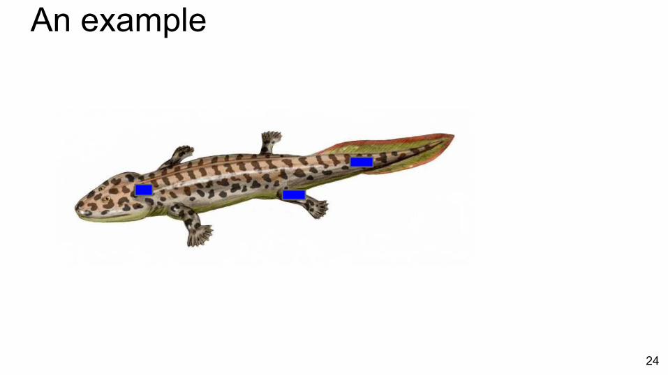
An example
Image: Nobu Tamura
24
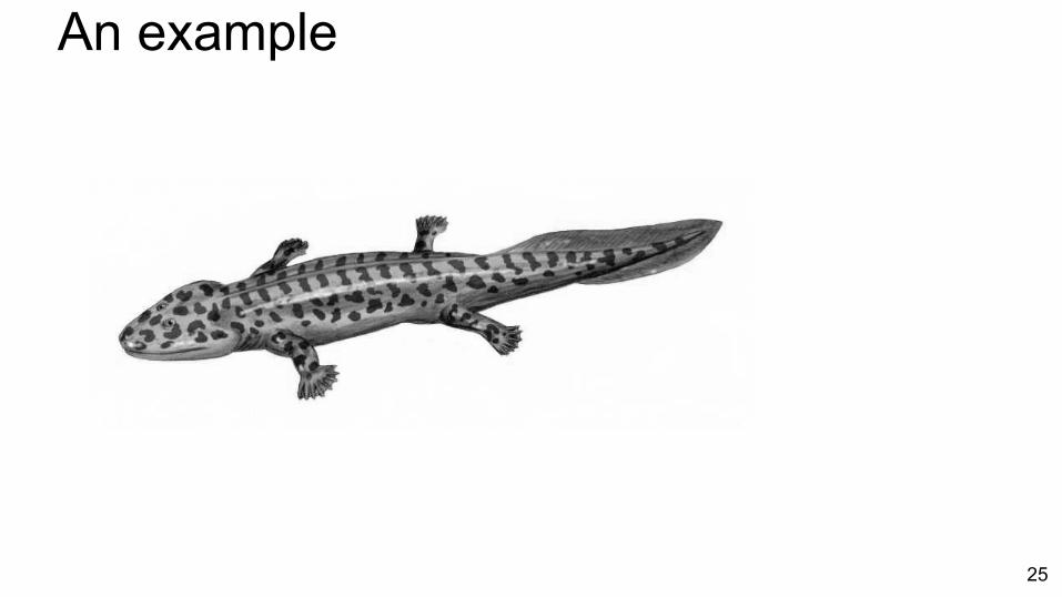
An example
Image: Nobu Tamura
25
An example
Image: Nobu Tamura
26
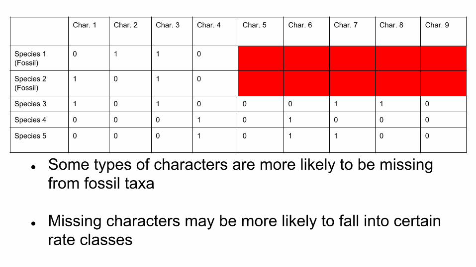
● Some types of characters are more likely to be missing from fossil taxa
● Missing characters may be more likely to fall into certain rate classes
Char. 1 Char. 2 Char. 3 Char. 4 Char. 5 Char. 6 Char. 7 Char. 8 Char. 9
Species 1(Fossil)
0 1 1 0 ? ? ? ? ?
Species 2(Fossil)
1 0 1 0 ? ? ? ? ?
Species 3 1 0 1 0 0 0 1 1 0
Species 4 0 0 0 1 0 1 0 0 0
Species 5 0 0 0 1 0 1 1 0 0
Missing data
● In these conditions, some model assumptions have been violated
● Given these model violations, is it preferable to use parsimony?
28
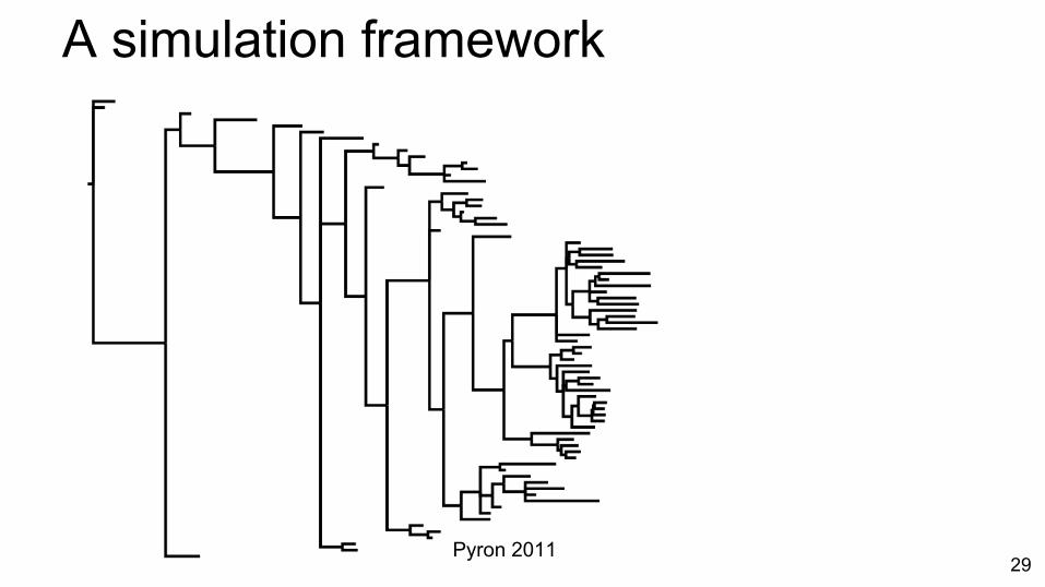
A simulation framework
Pyron 201129
A simulation framework
● Simulate characters along the tree from the previous slide
30
A simulation framework
● Simulate characters
○ 350 & 1000 character data sets
31
A simulation framework
● Simulate characters
○ 350 & 1000 character data sets
● Estimate topology using the Mk model and parsimony
32
Rate heterogeneity
● Different rates of character evolution
○ Low rates of change mean each character is likely to have changed rarely, if at all
○ High rates mean there are likely reversals and parallel evolution in the data
33
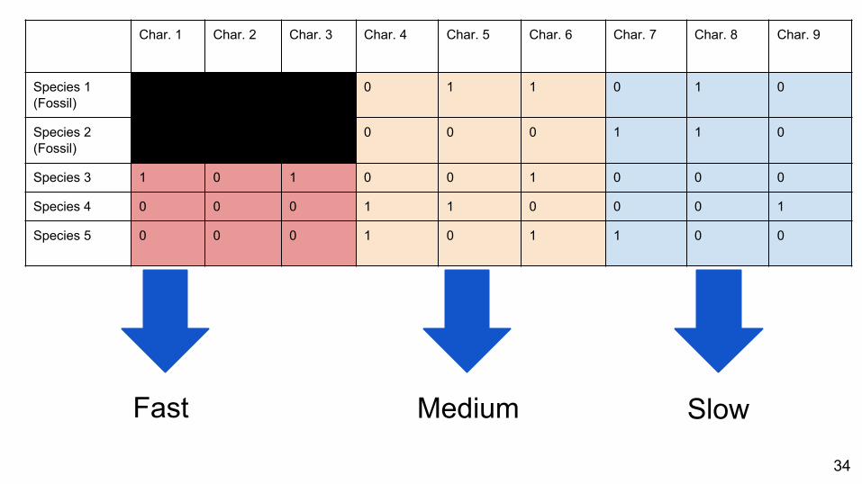
Fast Medium Slow
Char. 1 Char. 2 Char. 3 Char. 4 Char. 5 Char. 6 Char. 7 Char. 8 Char. 9
Species 1(Fossil)
? ? ? 0 1 1 0 1 0
Species 2(Fossil)
? ? ? 0 0 0 1 1 0
Species 3 1 0 1 0 0 1 0 0 0
Species 4 0 0 0 1 1 0 0 0 1
Species 5 0 0 0 1 0 1 1 0 0
34
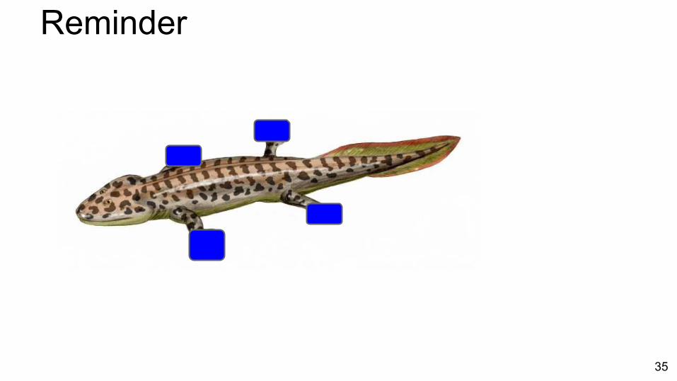
Reminder
Image: Nobu Tamura
35
Rate heterogeneity
● Diversity of rate classes can be helpful for resolving different regions of phylogenetic trees
○ Likelihood models account for superimposed changes
36
Rate heterogeneity
● Diversity of rate classes can be helpful for resolving different regions of phylogenetic trees○ Likelihood models account for superimposed
changes○ In analysis, rate heterogeneity is often modeled as
gamma-distributed
37
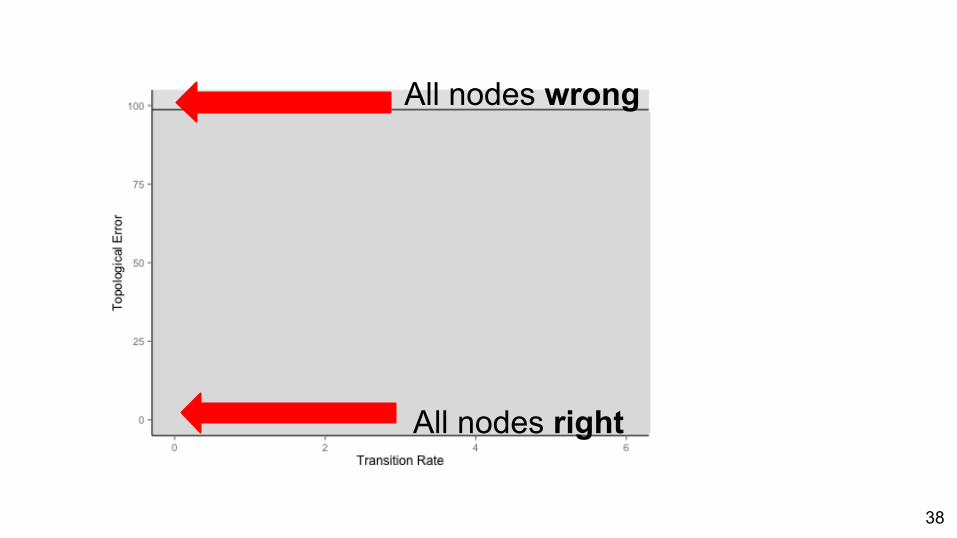
ResultsAll nodes wrong
All nodes right
38
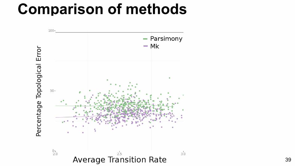
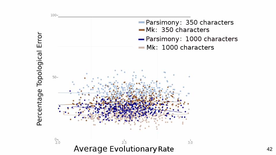
Comparison of methods
39
Per
cent
age
Topo
logi
cal E
rror
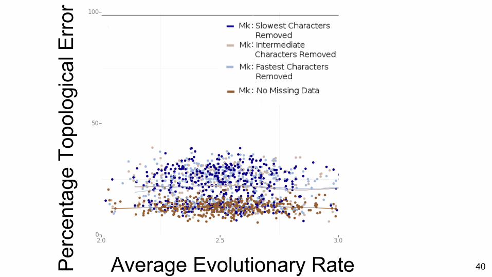
Average Evolutionary Rate 40
Per
cent
age
Topo
logi
cal E
rror
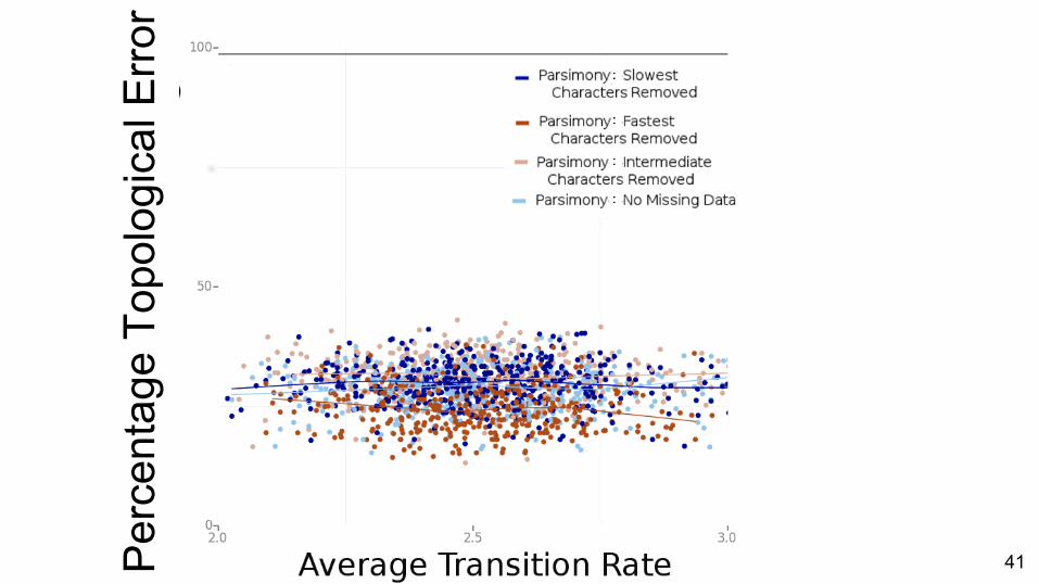
41
42
Summary - Chapter One
Does a parametric approach (Mk) outperform non-parametric approach
(parsimony) when model assumptions are violated?
43
Summary - Chapter One
Does a parametric approach (Mk) outperform non-parametric approach (parsimony) when
model assumptions are violated?Yes
44
Summary - Chapter One
Caveats: We’ve really only looked at one type of model violation here
There are other reasons you might use parsimony, or might think the contrast of
likelihood and parsimony methods is telling you something interesting
45
Chapter Two: Modeling character change heterogeneity through the use of priors
46
Model Assumptions
● Change is symmetrical between states
47
Model Assumptions
● Change is symmetrical between states○ We know this is not always true
48
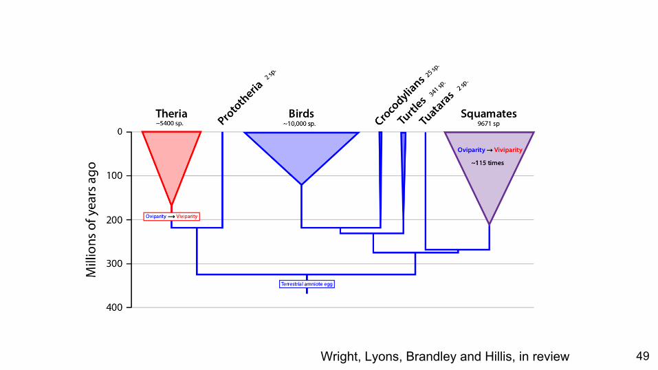
Wright, Lyons, Brandley and Hillis, in review 49
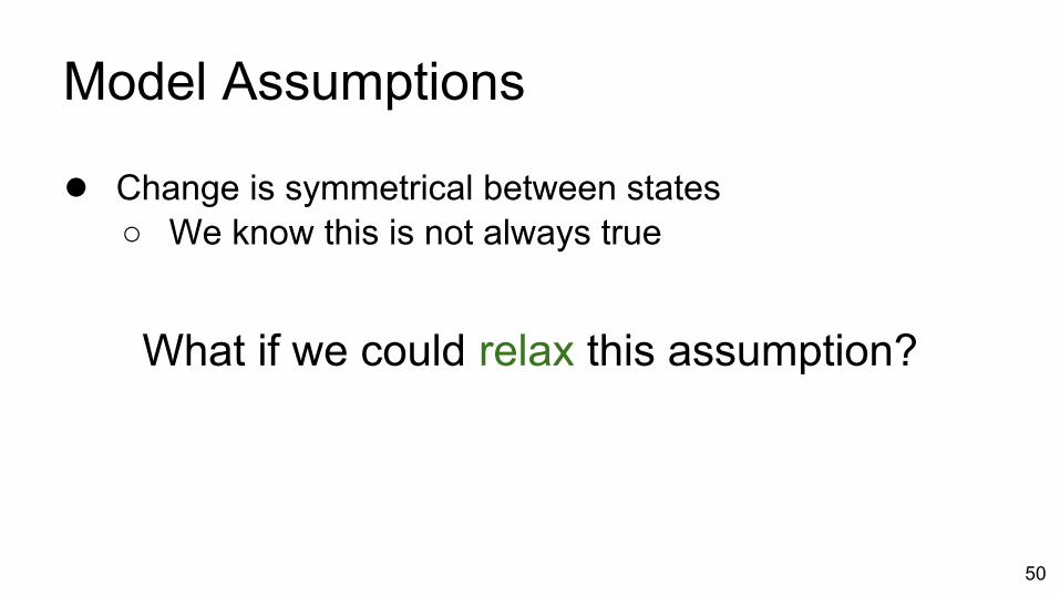
Model Assumptions
● Change is symmetrical between states○ We know this is not always true
What if we could relax this assumption?
50
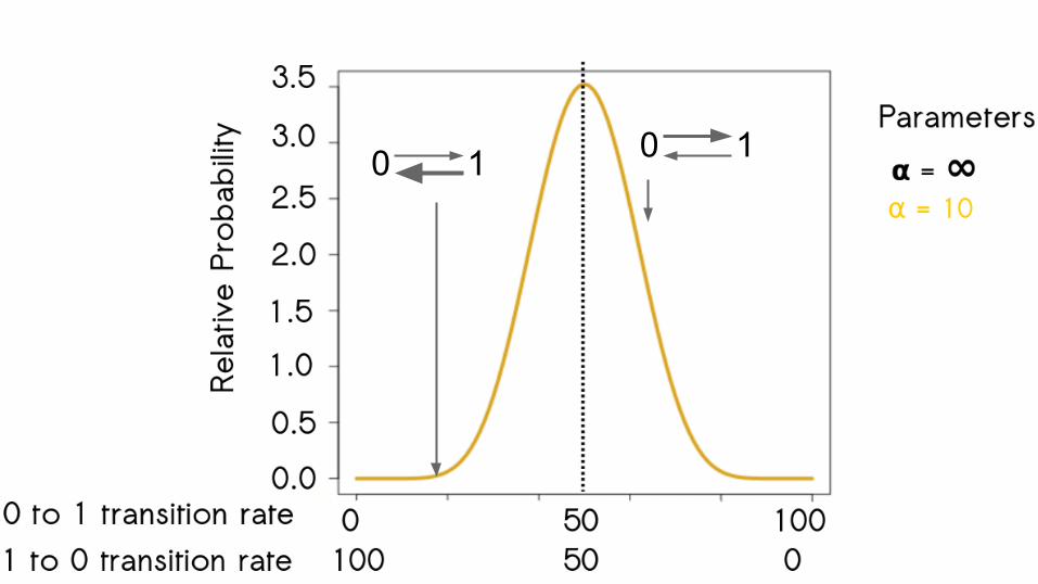
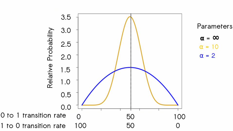
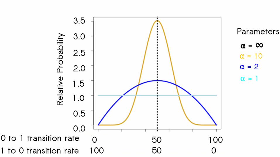
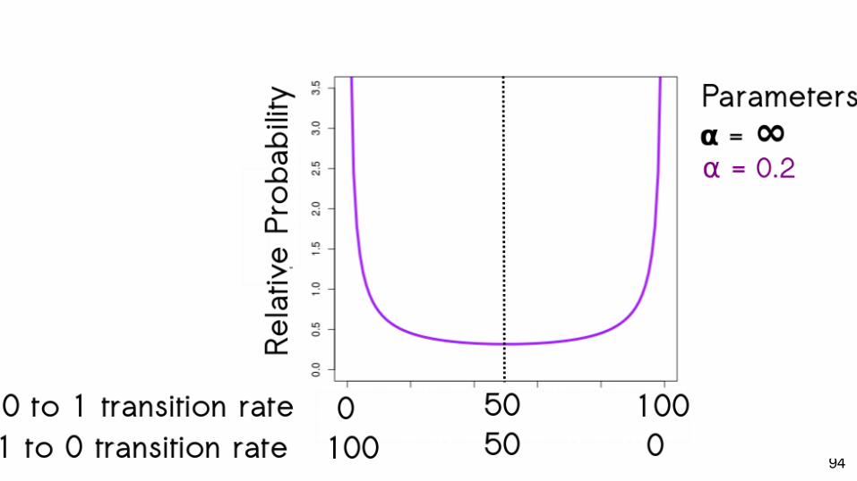
Relaxing this assumption
● In Bayesian estimation, we can put priors on the parameters in our analyses
51
Relaxing this assumption
● In Bayesian estimation, we can put priors on the parameters in our analyses
● Transition probabilities are the product of exchangeabilities and frequencies
52

Relaxing this assumption
53
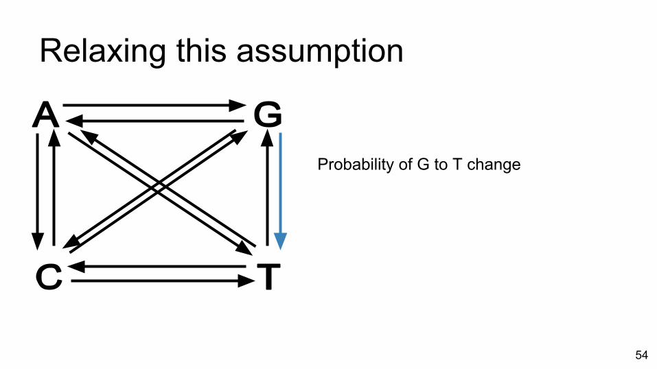
Relaxing this assumption
Probability of G to T change
54
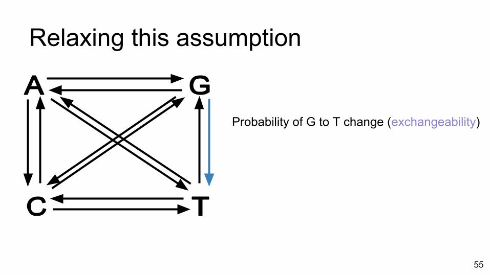
Relaxing this assumption
Probability of G to T change (exchangeability)
55
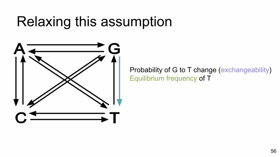
Relaxing this assumption
Probability of G to T change (exchangeability)Equilibrium frequency of T
56
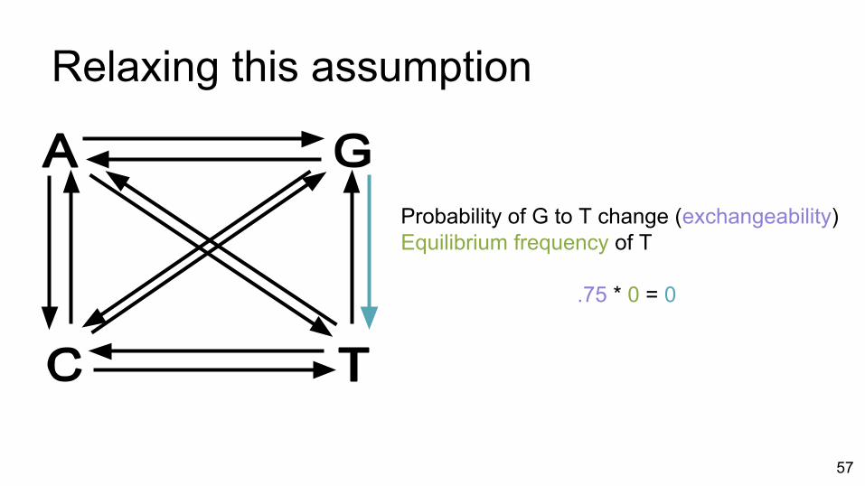
Relaxing this assumption
Probability of G to T change (exchangeability)Equilibrium frequency of T
.75 * 0 = 0
57
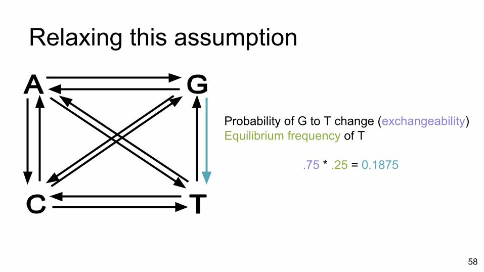
Relaxing this assumption
Probability of G to T change (exchangeability)Equilibrium frequency of T
.75 * .25 = 0.1875
58
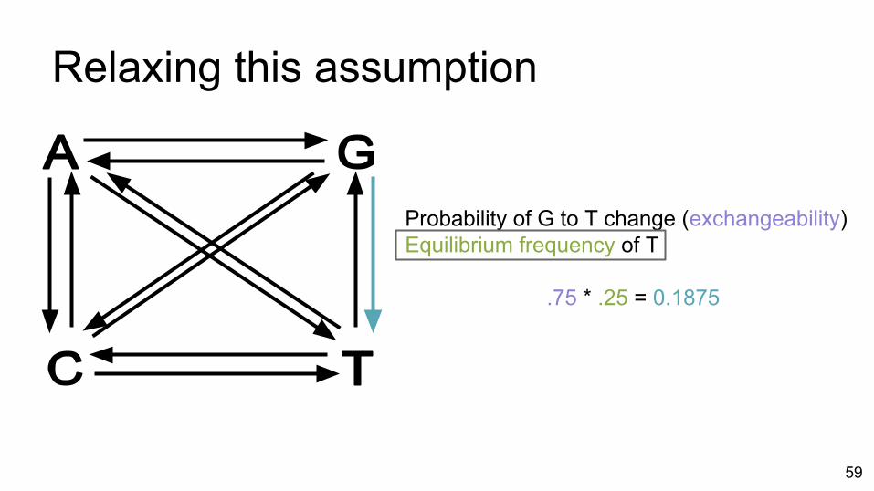
Relaxing this assumption
Probability of G to T change (exchangeability)Equilibrium frequency of T
.75 * .25 = 0.1875
59
60
61
62
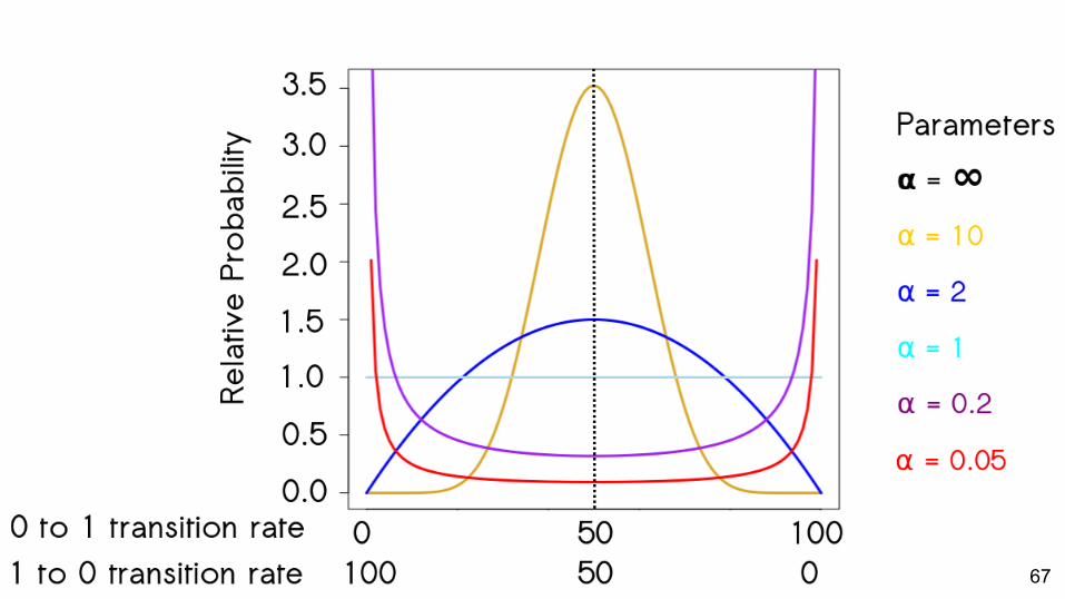
0 1
63
0 1 0 1
64
65
66
67
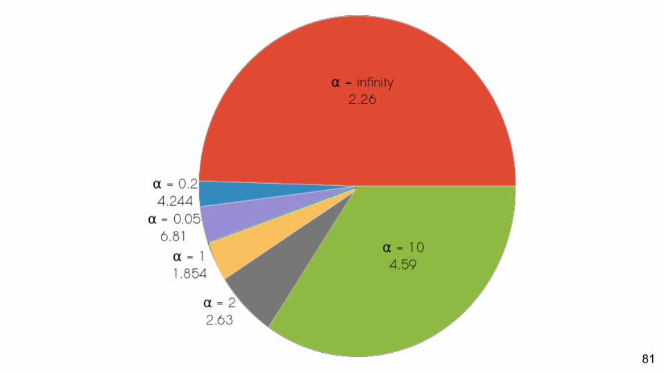
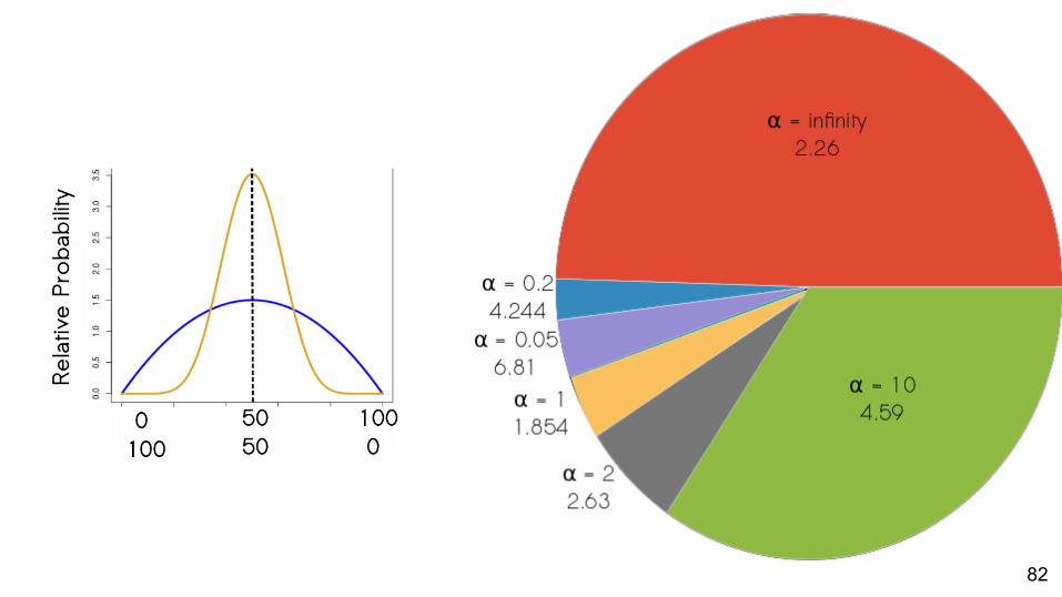
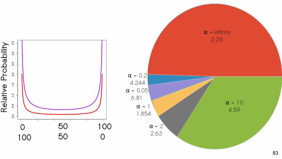
Empirical Datasets
● 206 datasets○ 5 to 279 taxa○ 11 to 364 characters○ Biased towards vertebrates
68
Empirical Datasets
● 206 datasets○ 5 to 279 taxa○ 11 to 364 characters○ Biased towards vertebrates
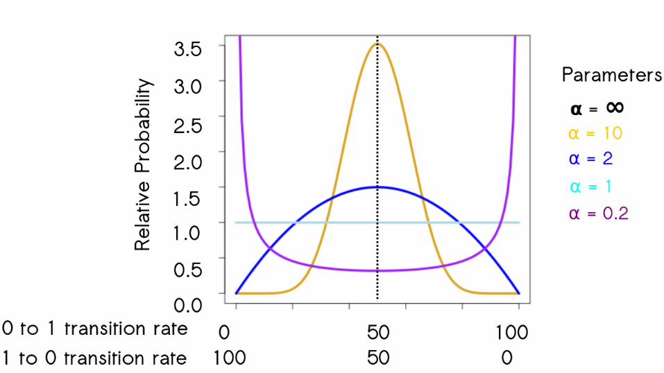
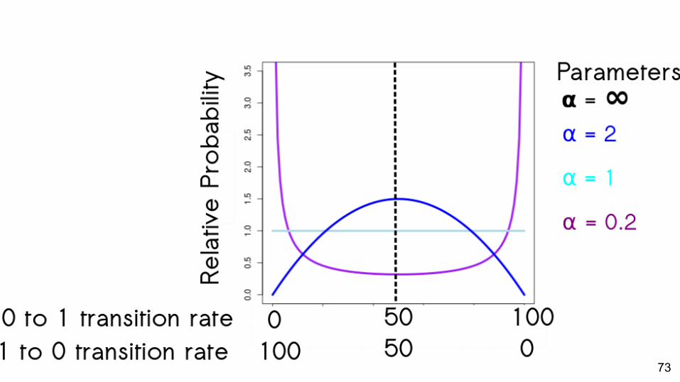
● Modeled character change asymmetry according to the 6 distributions
69

70

Empirical Datasets
Which priors best match empirical data?Does using the best-fit prior matter to
phylogenetic inference?
71
Simulations
● Simulated data according to 4 distributions○ Modeled the data according to each of the four
distributions
72
73
Simulations
● Simulated data according to 4 distributions○ Modeled the data according to each of the four
distributions○ One generating model, 3 misspecified models
74
75
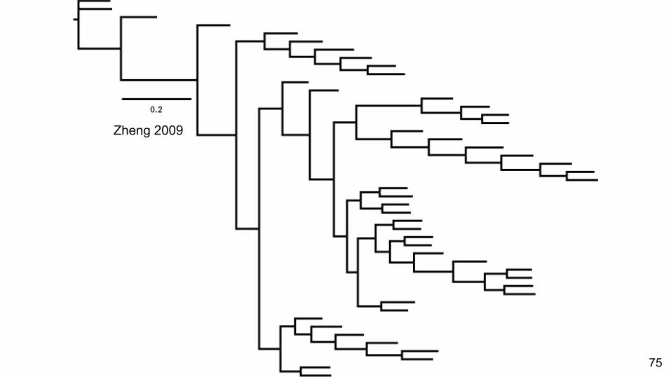
Zheng 2009
76
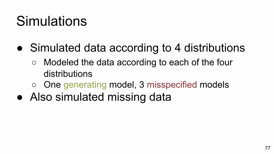
Simulations
● Simulated data according to 4 distributions○ Modeled the data according to each of the four
distributions○ One generating model, 3 misspecified models
● Also simulated missing data
77
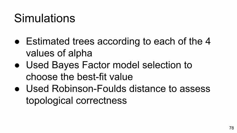
Simulations
● Estimated trees according to each of the 4 values of alpha
● Used Bayes Factor model selection to choose the best-fit value
● Used Robinson-Foulds distance to assess topological correctness
78
Simulations
Can we detect the generating value of alpha among misspecified values of alpha?
Does using the correct alpha result in a more correct tree?
79
Empirical - Results
80
81
82
83
Empirical Datasets
Which priors best match empirical data?About half: best fit is the α = ∞ prior
Strength of support for different values of α varies
84
Empirical Datasets
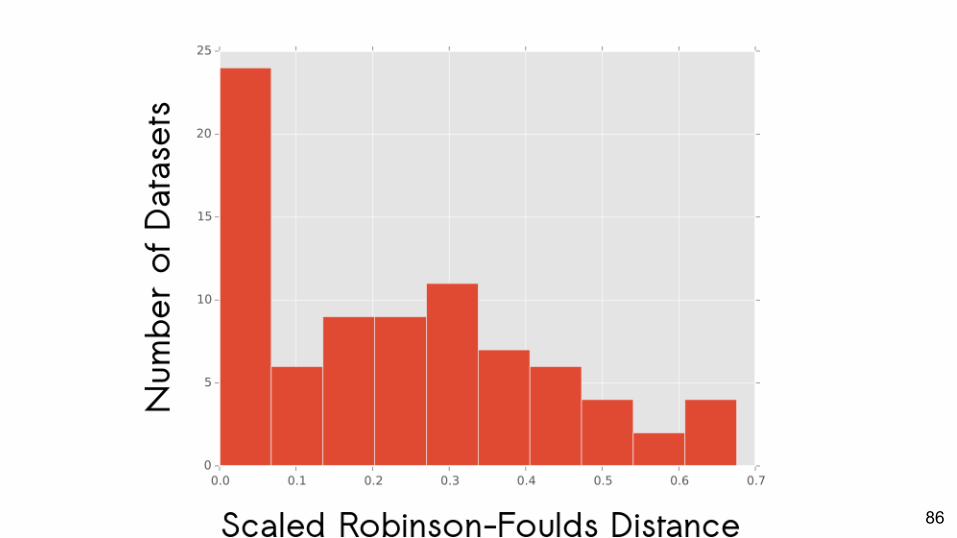
Does using the best-fit prior matter to phylogenetic inference?
85
86
Empirical Datasets
Does using the best-fit prior matter to phylogenetic inference?
Variable.
87
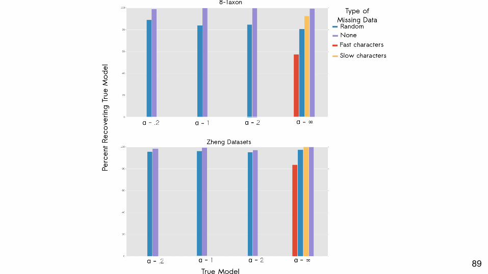
Simulated Datasets
Can we detect the generating value of α among misspecified values of α?
88
89
Simulated Data
Can we detect the generating value of α among misspecified values of α?
Yes.
90
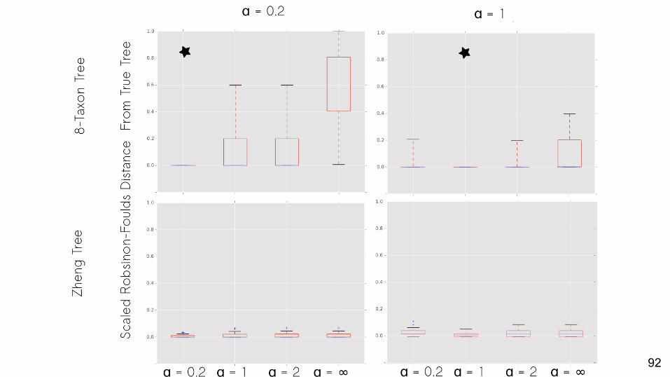
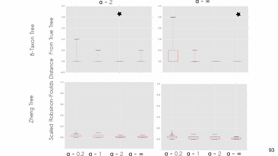
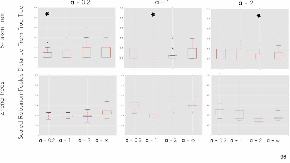
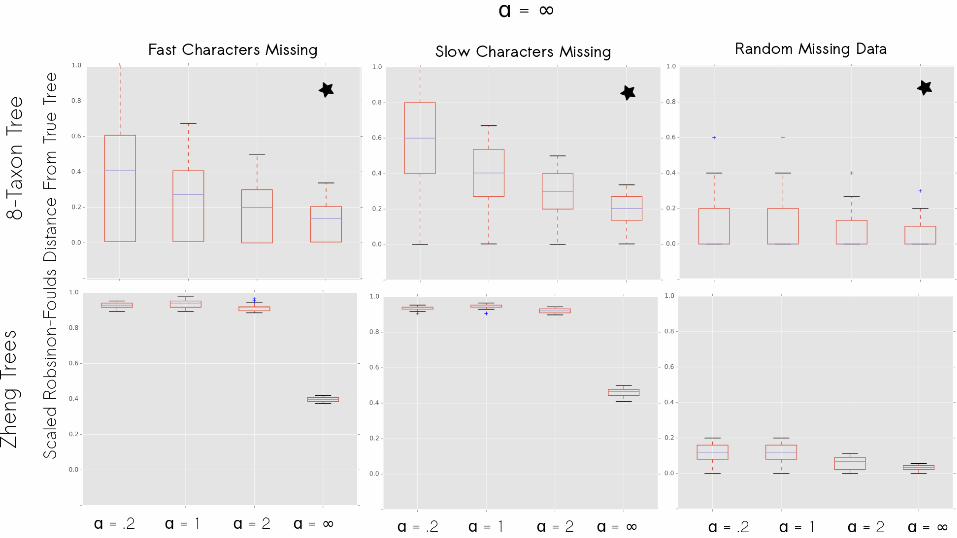
Simulated Data
Does using the best-fit α result in a more correct tree?
91
Sca
led
Rob
inso
n-Fo
ulds
Dis
tanc
e to
Tru
e Tr
ee
Zheng Trees8-Taxon
92
93
94
Simulations
Does using the best-fit alpha result in a more correct tree?
No missing data: Yes.
95
96
Analytical Model97
Simulations
Does using the best-fit α result in a more correct tree?
Yes, and the importance of doing so is greater when the problem is harder
98
Chapter Two: Conclusions
● Appropriate fit of α parameter improves phylogenetic estimation
● Bayes Factor model selection performs well at choosing the best-fit value of α among a set of α values
99

Chapter Three: Use of an Automated Method for Partitioning Morphological Data
100
Partitioning
● Refers to breaking a dataset into smaller subsets that can be analyzed under different phylogenetic models
101
Partitioning
● Refers to breaking a dataset into smaller subsets that can be analyzed under different phylogenetic models○ Well-explored in a molecular context
102
Partitioning
● Refers to breaking a dataset into smaller subsets that can be analyzed under different phylogenetic models○ Well-explored in a molecular context (Brown and Lemmon
2007)
○ Often, partition schemes are tested as a stage in model-fitting
103
Partitioning
● Less well-explored in morphology
104
Partitioning
● Less well-explored in morphology○ Clarke and Middleton (2008) is one of the few
explorations of partitioning in a likelihood context for morphology
105
Partitioning
● Less well-explored in morphology○ Clarke and Middleton (2008) is one of the few
explorations of partitioning in a likelihood context for morphology
○ Used anatomical subregion partitioning
106
Partitioning
● Less well-explored in morphology○ Clarke and Middleton (2008) is one of the few
explorations of partitioning in a likelihood context for morphology
○ Used anatomical subregion partitioning○ Found improved model fit and different topology with
partitioned data
107
Partitioning
● Less well-explored in morphology○ Clarke and Middleton (2008) is one of the few
explorations of partitioning in a likelihood context for morphology
○ Used anatomical subregion partitioning○ Found improved model fit and different topology with
partitioned data
108
PartitionFinder Morphology
● Adaptation of technology for partitioning of genome-scale information
109
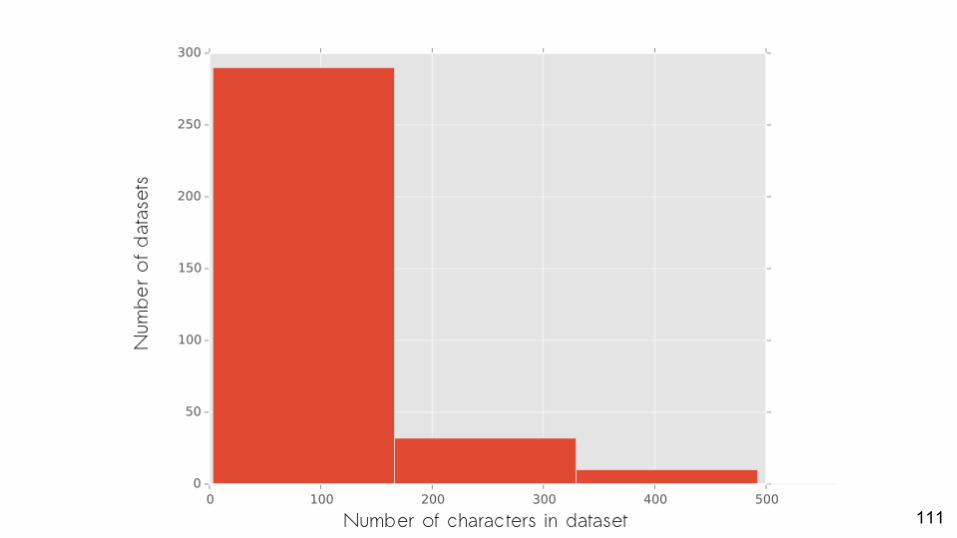
PartitionFinder Morphology
● Adaptation of technology for partitioning of genome-scale information○ But we don’t have genome-scale information
110
111
PartitionFinder Morphology
● Estimate a phylogenetic tree from the unpartitioned data matrix
112
PartitionFinder Morphology
● Estimate a phylogenetic tree from the unpartitioned data matrix
● Fit parameters of the evolutionary model to the whole dataset as a single set of sites
113
PartitionFinder Morphology
● Estimate a phylogenetic tree from the unpartitioned data matrix
● Fit parameters of the evolutionary model to the whole dataset as a single set of sites
● Calculate the score of the data given this model according to an information theoretic criterion (AIC, BIC or AICc)
114
PartitionFinder Morphology
● Generate rates of evolution for each site in the dataset
115
PartitionFinder Morphology
● Generate rates of evolution for each site in the dataset
● Use k-means clustering to split the subset in two based on these rates
116
PartitionFinder Morphology
● Generate rates of evolution for each site in the dataset
● Use k-means clustering to split the subset in two based on these rates
● Fit parameters of the model for these new subsets
117
PartitionFinder Morphology
● Calculate the score of this new partitioned data matrix according to the same information theoretic criterion used in step 3.
118
PartitionFinder Morphology
● Calculate the score of this new partitioned data matrix according to the same information theoretic criterion used in step 3.
● If smaller subsets are supported by this criterion, continue to divide them, repeating steps 5-7. If not, terminate the search.
119
PartitionFinder Morphology
Are partitioned models often the best-fit model for empirical datasets?
120
PartitionFinder Morphology
Are partitioned models often the best-fit model for empirical datasets?
When they are, does this make a difference to the tree estimated?
121
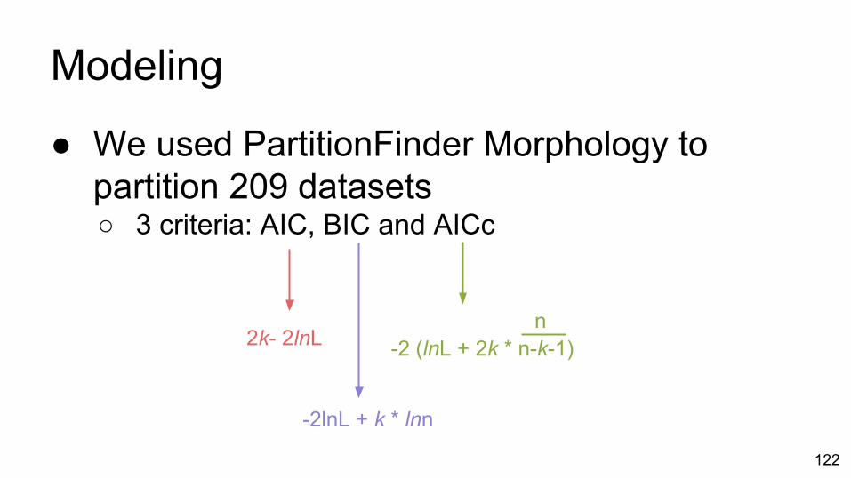
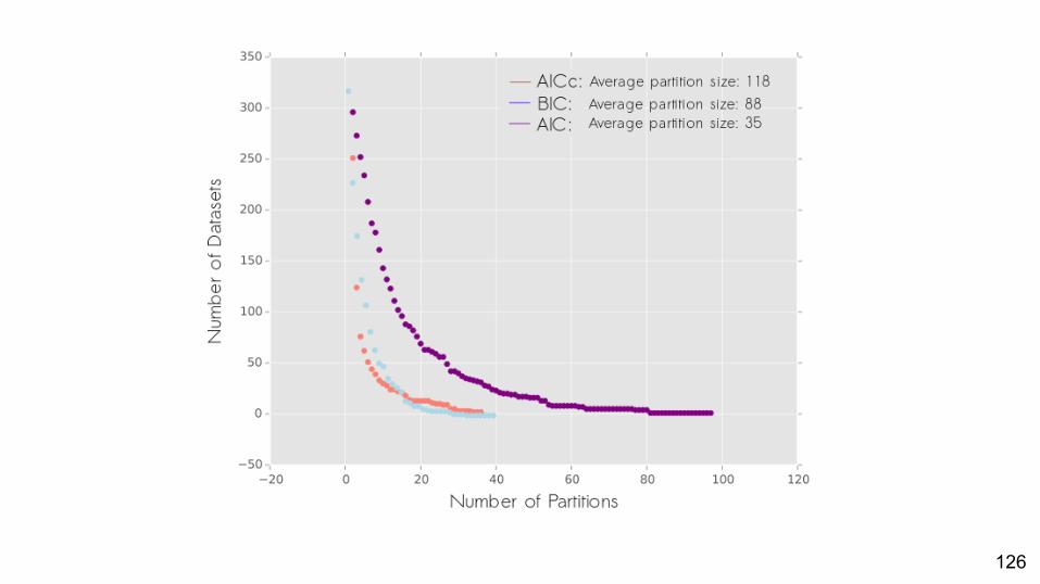
Modeling
● We used PartitionFinder Morphology to partition 209 datasets○ 3 criteria: AIC, BIC and AICc
2k- 2lnL -2 (lnL + 2k * n-k-1)
-2lnL + k * lnn
n
122
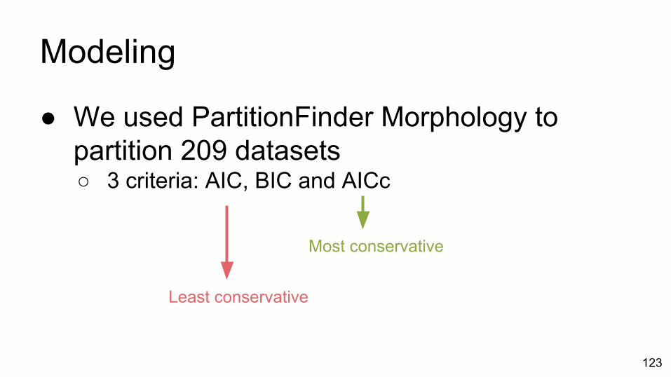
Modeling
● We used PartitionFinder Morphology to partition 209 datasets○ 3 criteria: AIC, BIC and AICc
Least conservative
Most conservative
123
Estimation
● Estimate trees under likelihood and Bayesian implementations of the Mk model using the partitioned data and unpartitioned data
124
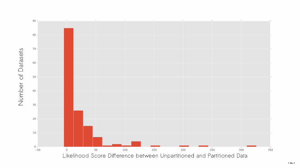
PartitionFinder Morphology
Are partitioned models often the best-fit model for empirical datasets?
125
126
127
128
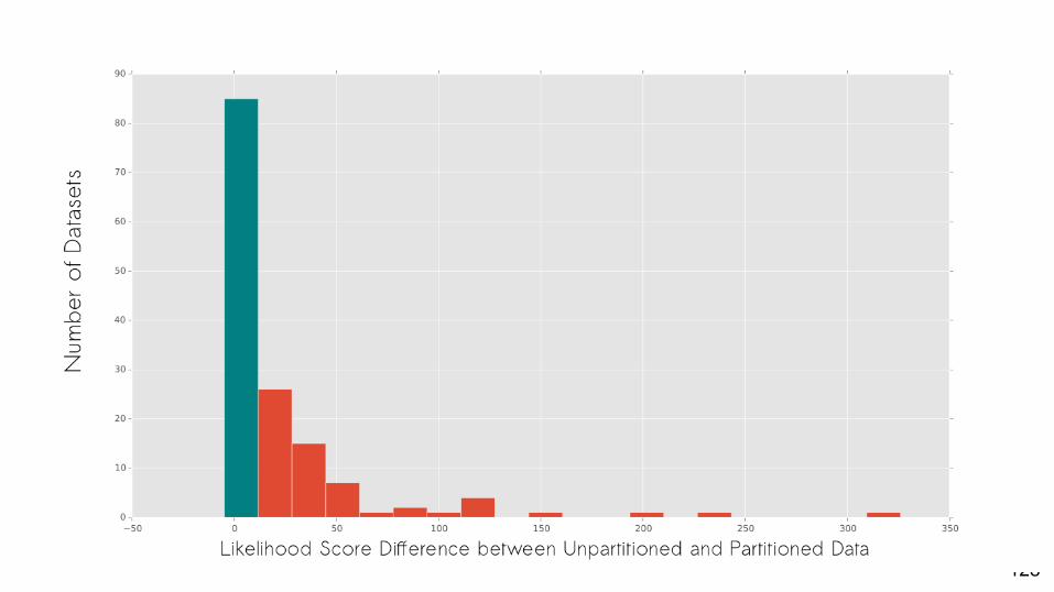
PartitionFinder Morphology
Are partitioned models often the best-fit model for empirical datasets?
Yes.
129
PartitionFinder Morphology
When a partitioned model is the best fit, does this make a difference to the tree estimated?
130
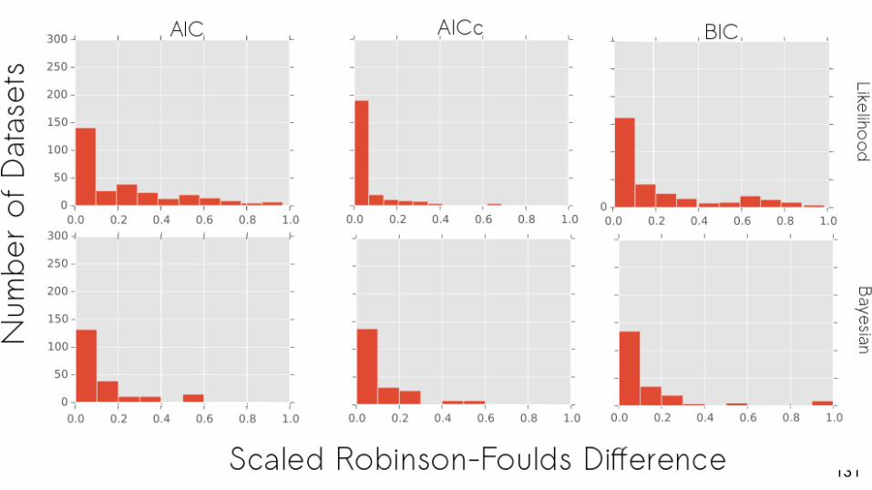
LikelihoodB
ayesian
Scaled Robinson-Foulds Distance
131
When a partitioned model is the best fit, does this make a difference to the tree estimated?
Yes, in empirical datasets we often estimate different trees.
132

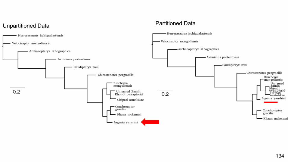
Specific Example
133
134
Unpartitioned Data Partitioned Data
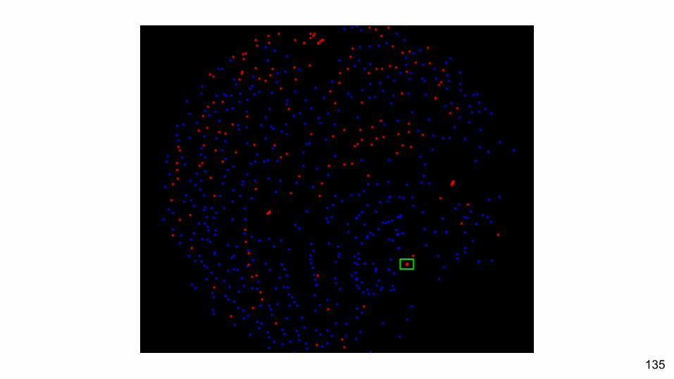
135
When a partitioned model is the best fit, does this make a difference to the tree estimated?
Yes, and the likelihood surface is more peaked.
136

Conclusions
137
Conclusions
● Chapter One: Likelihood-based methods are effective for estimating phylogeny for morphological data, even in the presence of biased missing data
138
Conclusions
● Chapter Two: Use of a prior on equilibrium state frequencies can improve the performance of Bayesian estimation using morphological data
139
Conclusions
● Chapter Three: PartitionFinder Morphology is a promising lead for evaluation of partitioning schemes
140

Thank you!CommitteeDavid HillisMartha SmithDavid CannatellaRandy LinderBob Jansen
LabmatesBen, Emily Jane, Thomas, Patricia, Becca, Mariana, Shannon, Patrick, Chris, J9, Matt, Sandi, Carlos, Taylor, Katie, Devon, Anne, Jim, Jeremy, Tracy
OtherUT vert paleo, especially Julia, Robert, Zach
And the people who make this worth doing:You know who you are.And Jason and unnamed baby girl Wright Stinnett.
Collaborators:Graeme Lloyd, Paul Fransden, David Bapst, Nick Matzke, Matt Brandley, Rob Lanfear
141