DeepStack: Expert-Level Artificial Intelligence inNo-Limit Poker

Matej Moravcık♠,♥,†, Martin Schmid♠,♥,†, Neil Burch♠, Viliam Lisy♠,♣,Dustin Morrill♠, Nolan Bard♠, Trevor Davis♠,

Kevin Waugh♠, Michael Johanson♠, Michael Bowling♠,∗♠Department of Computing Science, University of Alberta,

Edmonton, Alberta, T6G2E8, Canada♥Department of Applied Mathematics, Charles University,

Prague, Czech Republic♣Department of Computer Science, FEE, Czech Technical University,

Prague, Czech Republic

†These authors contributed equally to this work and are listed in alphabetical order.∗To whom correspondence should be addressed; E-mail: bowling@cs.ualberta.ca

Artificial intelligence has seen a number of breakthroughs in recent years, withgames often serving as significant milestones. A common feature of games withthese successes is that they involve information symmetry among the players,where all players have identical information. This property of perfect infor-mation, though, is far more common in games than in real-world problems.Poker is the quintessential game of imperfect information, and it has been alongstanding challenge problem in artificial intelligence. In this paper we in-troduce DeepStack, a new algorithm for imperfect information settings such aspoker. It combines recursive reasoning to handle information asymmetry, de-composition to focus computation on the relevant decision, and a form of intu-ition about arbitrary poker situations that is automatically learned from self-play games using deep learning. In a study involving dozens of participantsand 44,000 hands of poker, DeepStack becomes the first computer program tobeat professional poker players in heads-up no-limit Texas hold’em. Further-more, we show this approach dramatically reduces worst-case exploitabilitycompared to the abstraction paradigm that has been favored for over a decade.

Games have long served as a benchmark and set of milestones for progress in artificial

1

arX

iv:1

701.

0172

4v1

[cs

.AI]

6 J

an 2

017

intelligence. In the last two decades, we have seen computer programs reach a performance thatexceeds expert human players in many games, e.g., backgammon (1), checkers (2), chess (3),Jeopardy! (4), Atari video games (5), and go (6). These successes all involve games withinformation symmetry, where all players have identical information about the current state ofthe game. This property of perfect information is also at the heart of the algorithms that enabledthese successes, e.g., local search during play (7, 8).

The founder of modern game theory and computing pioneer, von Neumann, envisionedreasoning in games without perfect information. “Real life is not like that. Real life consists ofbluffing, of little tactics of deception, of asking yourself what is the other man going to thinkI mean to do. And that is what games are about in my theory.” (9) One game that fascinatedvon Neumann was poker, where players are dealt private cards and take turns making bets orbluffing on holding the strongest hand, calling opponents’ bets, or folding and giving up on thehand and the bets already added to the pot. Poker is a game of imperfect information, whereplayers’ private cards give them asymmetric information about the state of game.

There has been some AI success in heads-up (i.e., two-player) limit Texas hold’em, thesmallest variant of poker played by humans.1 However, heads-up limit Texas hold’em hasfewer than 1014 decision points. By comparison, computers have exceeded expert human per-formance in go (6), a perfect information game with approximately 10170 decision points (12).The comparable variant of poker is heads-up no-limit Texas hold’em (HUNL). In HUNL, thetwo players can bet any number of chips, resulting in over 10160 decision points (13).

Imperfect information games require more complex reasoning than their perfect informa-tion counterparts. The correct decision at a particular moment depends upon the probabilitydistribution over private information that the opponent holds, which is revealed through theirpast actions. However, how the opponent’s actions reveal that information depends upon theirknowledge of our private information and how our actions reveal it. This kind of recursive rea-soning is why one cannot easily reason about game situations in isolation, which is at the heartof local search methods for perfect information games. Competitive AI approaches in imper-fect information games typically reason about the entire game and produce a complete strategyprior to play (14, 15).2 Counterfactual regret minimization (CFR) (11, 14, 17) is one such tech-nique that uses self-play to do recursive reasoning through adapting its strategy against itselfover successive iterations. If the game is too large to be solved directly, the common solutionis to solve a smaller, abstracted game. To play the original game, one translates situations andactions from the original game in to the abstract game.

While this approach makes it feasible for programs to reason in a game like HUNL, it doesso by squeezing HUNL’s 10160 situations into the order of 1014 abstract situations. Likely

1In 2008, Polaris defeated a team of professional poker players in heads-up limit Texas hold’em (10). In 2015,Cepheus essentially solved the game (11).

2End-game solving (16–18) is one exception to computation occurring prior to play. When the game nears theend, a new computation is invoked over the remainder of the game. Thus, the program need not store this partof the strategy or can use a finer-grained abstraction aimed to improve the solution quality. We discuss this asre-solving when we introduce DeepStack’s new technique of continuous re-solving.

2

as a result of this loss of information, such programs are well behind expert human play. In2015, the computer program Claudico lost to a team of professional poker players by a marginof 91 mbb/g,3 which is a “huge margin of victory” (19) and significant at a 90% confidencelevel. Furthermore, it has been recently shown that abstraction-based programs from the AnnualComputer Poker Competition have massive flaws (20). Four such programs (including topprograms from the 2016 competition) were evaluated using a local best-response technique thatproduces an approximate lower-bound on how much a strategy can lose. All four abstraction-based programs are beatable by over 3,000 mbb/g, which is four times as large as simply foldingeach game.

DeepStack takes a fundamentally different approach. It continues to use the recursive rea-soning of CFR to handle information asymmetry. However, it does not compute and store acomplete strategy prior to play and so has no need for explicit abstraction. Instead it considerseach particular situation as it arises during play, but not in isolation. It avoids reasoning aboutthe entire remainder of the game by substituting the computation beyond a certain depth with afast approximate estimate. This estimate can be thought of as DeepStack’s intuition: a gut feel-ing of the value of holding any possible private cards in any possible poker situation. Finally,DeepStack’s intuition, much like human intuition, needs to be trained. We train it with deeplearning using examples generated from random poker situations. We show that DeepStackis theoretically sound, produces substantially less exploitable strategies than abstraction-basedtechniques, and is the first program to beat professional poker players at HUNL with a remark-able average win rate of over 450 mbb/g.

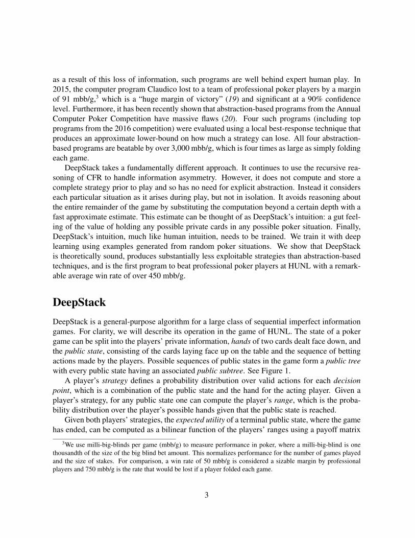
DeepStackDeepStack is a general-purpose algorithm for a large class of sequential imperfect informationgames. For clarity, we will describe its operation in the game of HUNL. The state of a pokergame can be split into the players’ private information, hands of two cards dealt face down, andthe public state, consisting of the cards laying face up on the table and the sequence of bettingactions made by the players. Possible sequences of public states in the game form a public treewith every public state having an associated public subtree. See Figure 1.

A player’s strategy defines a probability distribution over valid actions for each decisionpoint, which is a combination of the public state and the hand for the acting player. Given aplayer’s strategy, for any public state one can compute the player’s range, which is the proba-bility distribution over the player’s possible hands given that the public state is reached.

Given both players’ strategies, the expected utility of a terminal public state, where the gamehas ended, can be computed as a bilinear function of the players’ ranges using a payoff matrix

3We use milli-big-blinds per game (mbb/g) to measure performance in poker, where a milli-big-blind is onethousandth of the size of the big blind bet amount. This normalizes performance for the number of games playedand the size of stakes. For comparison, a win rate of 50 mbb/g is considered a sizable margin by professionalplayers and 750 mbb/g is the rate that would be lost if a player folded each game.

3

P R E - F L O P

F L O P

Raise

RaiseFoldCall

Call

Fold

Call

FoldCall

CallFold

BetCheck

Check

RaiseCheck

T U R N

-50

-100

100

100

-200

Fold

1

22

1

1

2 2

1

Figure 1: A portion of the public tree in HUNL. Red and turquoise edges represent playeractions. Green edges represent revealed public cards. Leaf nodes with chips represent theend of the game, where the payoff may be fixed if a player folded or determined by the jointdistribution of player hands given the preceding actions.

determined by the rules of the game. The expected utility of any other public state s, includingthe initial state, is the expected utility over terminal states reached given the players’ strate-gies. A best response strategy is one which maximizes a player’s expected utility against anopponent strategy. In two-player, zero-sum games like HUNL, a solution or Nash equilibriumstrategy (21) maximizes the expected utility when playing against a best response opponentstrategy. The exploitability of a strategy is the difference in expected utility against its bestresponse opponent and the expected utility under a Nash equilibrium.

The DeepStack algorithm seeks to compute and play a low-exploitability strategy for thegame, i.e., solve for an approximate Nash equilibrium. DeepStack computes this strategy dur-ing play4 and only for the states of the public tree that actually arise during play as illustratedin Figure 2. This local computation lets DeepStack reason in games that are too big for existingalgorithms without having to abstract the game’s 10160 decision points down to 1014 to makesolving tractable. The DeepStack algorithm is composed of three ingredients: a sound localstrategy computation for the current public state, depth-limited lookahead using a learned valuefunction over arbitrary poker situations, and a restricted set of lookahead actions. We explaineach ingredient in turn, starting with the local lookahead procedure that by itself is computa-tionally infeasible, before discussing the ingredients that make DeepStack tractable.

4While DeepStack’s strategy is computed during play, its strategy is static, albeit stochastic, since it is the resultof a deterministic computation that produces a probability distribution over the available actions.

4

(c)

Sampled poker situations

(b)(a)

Agent's possible actions

Lookahead tree

Current public state

Neural net [see (b)]

Action history

Game tree

Subtree

ValuesRanges

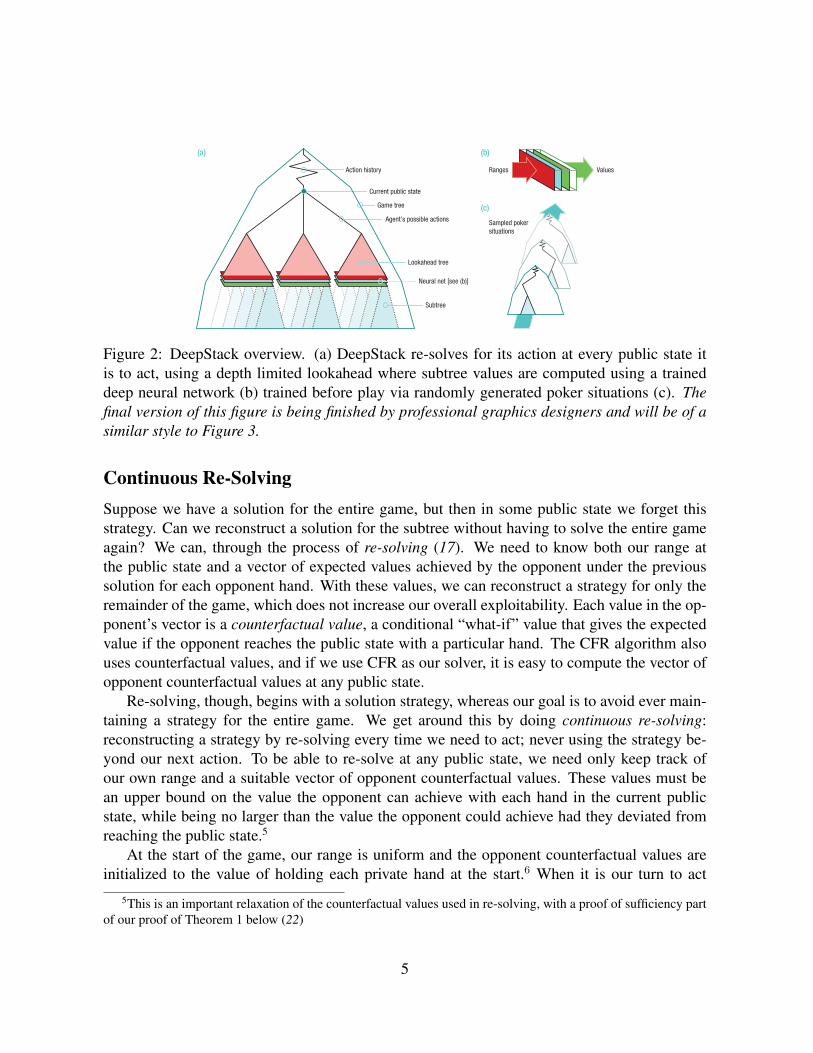
Figure 2: DeepStack overview. (a) DeepStack re-solves for its action at every public state itis to act, using a depth limited lookahead where subtree values are computed using a traineddeep neural network (b) trained before play via randomly generated poker situations (c). Thefinal version of this figure is being finished by professional graphics designers and will be of asimilar style to Figure 3.

Continuous Re-SolvingSuppose we have a solution for the entire game, but then in some public state we forget thisstrategy. Can we reconstruct a solution for the subtree without having to solve the entire gameagain? We can, through the process of re-solving (17). We need to know both our range atthe public state and a vector of expected values achieved by the opponent under the previoussolution for each opponent hand. With these values, we can reconstruct a strategy for only theremainder of the game, which does not increase our overall exploitability. Each value in the op-ponent’s vector is a counterfactual value, a conditional “what-if” value that gives the expectedvalue if the opponent reaches the public state with a particular hand. The CFR algorithm alsouses counterfactual values, and if we use CFR as our solver, it is easy to compute the vector ofopponent counterfactual values at any public state.

Re-solving, though, begins with a solution strategy, whereas our goal is to avoid ever main-taining a strategy for the entire game. We get around this by doing continuous re-solving:reconstructing a strategy by re-solving every time we need to act; never using the strategy be-yond our next action. To be able to re-solve at any public state, we need only keep track ofour own range and a suitable vector of opponent counterfactual values. These values must bean upper bound on the value the opponent can achieve with each hand in the current publicstate, while being no larger than the value the opponent could achieve had they deviated fromreaching the public state.5

At the start of the game, our range is uniform and the opponent counterfactual values areinitialized to the value of holding each private hand at the start.6 When it is our turn to act

5This is an important relaxation of the counterfactual values used in re-solving, with a proof of sufficiency partof our proof of Theorem 1 below (22)

5

we re-solve the subtree at the current public state using the stored range and opponent values,and act according to the computed strategy, discarding the strategy before we act again. Aftereach action — our own, our opponent’s, and chance — we update our range and opponentcounterfactual values according to the following rules:

• Own Action. Replace the opponent counterfactual values with those computed in the re-solved strategy for our chosen action. Update our own range using the computed strategyand Bayes’ rule.

• Chance Action. Replace the opponent counterfactual values with those computed forthis chance action from the last re-solve. Update our own range by zeroing hands in therange that are impossible given any new public cards.

• Opponent Action. Do nothing.

These updates ensure the opponent counterfactual values satisfy our sufficient conditions, andthe whole procedure produces arbitrarily close approximations of a Nash equilibrium (see The-orem 1). Notice that continuous re-solving never keeps track of the opponent’s range, insteadonly keeping track of counterfactual values. Furthermore, it never requires knowledge of theopponent’s action to update these values, which is an important difference from traditional re-solving. Both will prove key to making this algorithm efficient and avoiding any need for thetranslation step required with action abstraction methods (23, 24).

Limited Lookahead and Sparse TreesContinuous re-solving is theoretically sound, but also impractical. While it does not ever main-tain a complete strategy, re-solving itself is intractable except near the end of the game. Forexample, re-solving for the first action would require temporarily computing an approximatesolution for the whole game. In order to make continuous re-solving practical, we need thesecond and third ingredients of DeepStack.

Limited Depth Lookahead via Intuition. When using CFR to solve or re-solve games, eachplayer’s strategy is improved locally on each iteration to smoothly approach a best-response. Inany public subtree(s), we could replace the iterative improvement with an explicit best-response.Using explicit best-responses for both players means computing a Nash equilibrium strategy forthese subtrees on each iteration. This results in CFR-D (17), a game solving algorithm that savesspace by not requiring subtree strategies (for example, in public states exceeding a fixed depth)to be stored. However, it increases computation time by requiring the subtree strategies berecomputed on each iteration when only the vector of counterfactual values are needed.

Instead of solving subtrees to get the counterfactual values, DeepStack uses a learned valuefunction intended to return an approximation of the values that would have been returned bysolving. The inputs to this function are the ranges for both players, the current pot size, and the

6

public cards. The outputs are a vector for each player containing the counterfactual values ofholding each hand in that situation. In other words, the input is itself a description of a pokergame: the probability distribution of being dealt individual private hands, the stakes of thegame, and any public cards revealed; the output is an estimate of how valuable holding certaincards would be in such a game. The value function is a sort of intuition, a fast estimate of thevalue of finding oneself in an arbitrary poker situation. Limiting the lookahead to depth four,and using a value function for all public states exceeding that depth, reduces the size of gamefor re-solving from 10160 decision points down to no more than 1017 decision points. DeepStackuses a deep neural network to approximate this function, which is described later.

A simpler form of using value functions to limit lookahead is at the heart of algorithms forperfect information games. Deep Blue searched to a minimum depth of 12 moves on average,with some lines searching much deeper, before applying an evaluation function at positionsbeyond that depth (3). AlphaGo at shallow depths combined Monte Carlo rollout evaluationswith the results of a trained evaluation function (6). In both cases the evaluation function neededto only return a single value given a single position in the game. DeepStack’s value functionmust be able to provide a vector of values given a probability distribution over positions in thegame.

Sound Reasoning. DeepStack’s depth-limited continuous re-solving is sound. If DeepStack’sintuition is “good” and “enough” computation is used in each re-solving step, then DeepStackplays an arbitrarily close approximation to a Nash equilibrium.

Theorem 1 If the values returned by the value function used when the depth limit is reachedhas error less than ε, and T iterations of CFR is used to re-solve, then the resulting strategy’sexploitability is less than k1ε+ k2/

√T , where k1 and k2 are game-specific constants. (22)

Sparse Lookahead Trees. The final ingredient in DeepStack is the reduction in the number ofactions considered so as to construct a sparse lookahead tree. DeepStack builds the lookaheadtree using only the actions fold (if valid), call, 2 or 3 bet/raise actions, and all-in. While thisstep loses the soundness property of Theorem 1 it moves DeepStack’s re-solving time into therange of conventional human play. With sparse and depth limited lookahead trees, the re-solvedgames have approximately 107 decision points, and can be solved in under five seconds.6

While this ingredient looks very similar to action abstraction (23,24), which often results inhighly exploitable strategies (20), there are important distinctions. Each re-solve in DeepStackstarts from the actual public state and so always knows the exact size of the pot. Second, thealgorithm never uses the opponent’s actual action to update its range or the opponent counter-factual values, and so no translation of opponent bets are ever needed.

6We also use our sparse and depth limited lookahead computation to solve for the opponent’s counterfactualvalues at the start of the game, which are used to initialize DeepStack’s continuous re-solving.

7

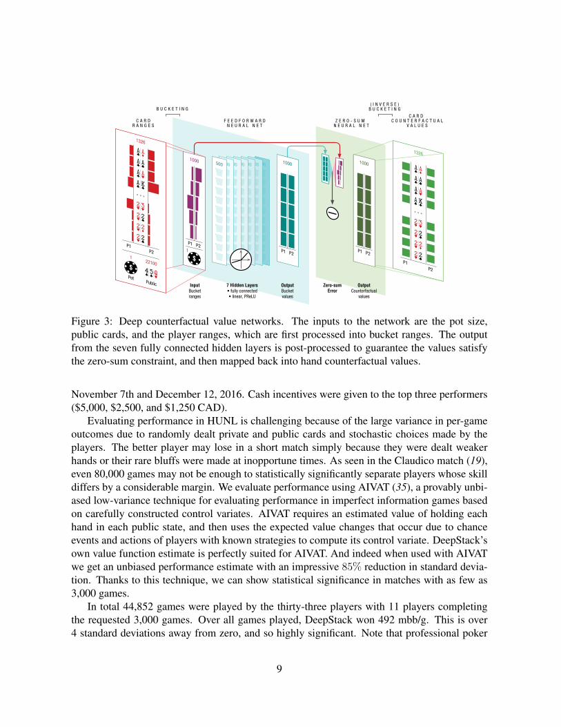
Deep Counterfactual Value NetworksDeep neural networks (DNNs) have proven to be powerful models and are responsible for ma-jor advances in image and speech recognition (25, 26), automated generation of music (27),and game-playing (5, 6). DeepStack uses DNNs, with a tailor-made architecture, as the valuefunction for its depth-limited lookahead. See Figure 3. Two separate networks are trained: oneestimates the counterfactual values after the first three public cards are dealt (flop network), theother after dealing the fourth public card (turn network). An auxiliary network for values beforeany public cards are dealt is used to speed up the re-solving for early actions (22).

Architecture. DeepStack uses a standard feed-forward network with seven fully connectedhidden layers each with 500 nodes and parametric rectified linear units (28) for the output. Thisbasic architecture is embedded in an outer network that guarantees the counterfactual valuessatisfy the zero-sum property. The outer computation takes the estimated counterfactual values,and computes a weighted sum using the two players’ input ranges resulting in separate estimatesof the game value. These two values should sum to zero, but may not. Half the actual sum isthen subtracted from the two players’ estimated counterfactual values. This entire computationis differentiable and can be trained with gradient descent. The network’s inputs are the pot-sizeas a fraction of the players’ total stacks and an encoding of the players’ ranges as a functionof the public cards. The ranges are encoded by bucketing hands, as in traditional abstractionmethods (29–31), and input as a vector of probabilities over the buckets. Note that while thisbucketing results in some loss of information, it is only used to estimate counterfactual valuesat the end of a lookahead tree rather than limiting what information the player has about theircards when acting. The output of the network are vectors of counterfactual values for eachplayer and hand, interpreted as fractions of the pot size.

Training. The turn network was trained by solving 10 million randomly generated poker turngames. These turn games used randomly generated ranges (22), public cards, and a randompot size. The target counterfactual values for each training game were generated by solvingthe game with players’ actions restricted to fold, call, a pot-sized bet, and an all-in bet, but nocard abstraction. The flop network was trained similarly with 1 million randomly generatedflop games. However, the target counterfactual values were computed using our limited-depthsolving procedure and our trained turn network. The networks were trained using the Adamgradient descent optimization procedure (32) with a Huber loss (33).

Evaluating DeepStackWe evaluated DeepStack by playing it against a pool of professional poker players recruitedby the International Federation of Poker (34). Thirty-three players from 17 countries wererecruited. Each was asked to complete a 3,000 game match over a period of four weeks between

8

InputBucketranges

7 Hidden Layers• fully connected• linear, PReLU

OutputBucketvalues

F E E D F O R W A R DN E U R A L N E T

Z E R O - S U M N E U R A L N E T

OutputCounterfactual

values

C A R D C O U N T E R F A C T U A L

V A L U E S

Zero-sumError

B U C K E T I N G( I N V E R S E )

B U C K E T I N G

C A R D R A N G E S

5005005005005005005001000

1P2P1

P1P2

1326

P1P2

PotPublic

1326

221001

1000

P2P1

1000

P2P1

Figure 3: Deep counterfactual value networks. The inputs to the network are the pot size,public cards, and the player ranges, which are first processed into bucket ranges. The outputfrom the seven fully connected hidden layers is post-processed to guarantee the values satisfythe zero-sum constraint, and then mapped back into hand counterfactual values.

November 7th and December 12, 2016. Cash incentives were given to the top three performers($5,000, $2,500, and $1,250 CAD).

Evaluating performance in HUNL is challenging because of the large variance in per-gameoutcomes due to randomly dealt private and public cards and stochastic choices made by theplayers. The better player may lose in a short match simply because they were dealt weakerhands or their rare bluffs were made at inopportune times. As seen in the Claudico match (19),even 80,000 games may not be enough to statistically significantly separate players whose skilldiffers by a considerable margin. We evaluate performance using AIVAT (35), a provably unbi-ased low-variance technique for evaluating performance in imperfect information games basedon carefully constructed control variates. AIVAT requires an estimated value of holding eachhand in each public state, and then uses the expected value changes that occur due to chanceevents and actions of players with known strategies to compute its control variate. DeepStack’sown value function estimate is perfectly suited for AIVAT. And indeed when used with AIVATwe get an unbiased performance estimate with an impressive 85% reduction in standard devia-tion. Thanks to this technique, we can show statistical significance in matches with as few as3,000 games.

In total 44,852 games were played by the thirty-three players with 11 players completingthe requested 3,000 games. Over all games played, DeepStack won 492 mbb/g. This is over4 standard deviations away from zero, and so highly significant. Note that professional poker

9

5 10 15 20 25 30

Participant

500

250

050

250

500

750

1000

1250

DeepSta

ck w

in r

ate

(m

bb/g

)

0

1000

2000

3000

Hands

pla

yed

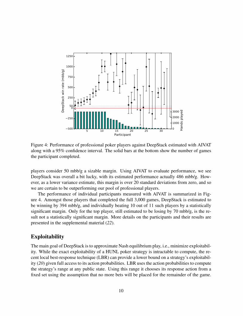
Figure 4: Performance of professional poker players against DeepStack estimated with AIVATalong with a 95% confidence interval. The solid bars at the bottom show the number of gamesthe participant completed.

players consider 50 mbb/g a sizable margin. Using AIVAT to evaluate performance, we seeDeepStack was overall a bit lucky, with its estimated performance actually 486 mbb/g. How-ever, as a lower variance estimate, this margin is over 20 standard deviations from zero, and sowe are certain to be outperforming our pool of professional players.

The performance of individual participants measured with AIVAT is summarized in Fig-ure 4. Amongst those players that completed the full 3,000 games, DeepStack is estimated tobe winning by 394 mbb/g, and individually beating 10 out of 11 such players by a statisticallysignificant margin. Only for the top player, still estimated to be losing by 70 mbb/g, is the re-sult not a statistically significant margin. More details on the participants and their results arepresented in the supplemental material (22).

ExploitabilityThe main goal of DeepStack is to approximate Nash equilibrium play, i.e., minimize exploitabil-ity. While the exact exploitability of a HUNL poker strategy is intractable to compute, the re-cent local best-response technique (LBR) can provide a lower bound on a strategy’s exploitabil-ity (20) given full access to its action probabilities. LBR uses the action probabilities to computethe strategy’s range at any public state. Using this range it chooses its response action from afixed set using the assumption that no more bets will be placed for the remainder of the game.

10

Thus it best-responds locally to the opponent’s actions, providing a lower-bound on their overallexploitability. As already noted, abstraction-based programs from the Annual Computer PokerCompetition are highly exploitable by LBR: four times more exploitable than folding everygame. However, even under a variety of settings, LBR fails to exploit DeepStack at all — itselflosing by over 350 mbb/g to DeepStack (22). Either a more sophisticated lookahead is requiredto identify its weaknesses or DeepStack is substantially less exploitable.

DiscussionDeepStack is the first computer program to defeat professional poker players at heads-up no-limit Texas Hold’em, an imperfect information game with 10160 decision points. Notably itachieves this goal with almost no domain knowledge or training from expert human games. Theimplications go beyond just being a significant milestone for artificial intelligence. DeepStackis a paradigmatic shift in approximating solutions to large, sequential imperfect informationgames. Abstraction and offline computation of complete strategies has been the dominant ap-proach for almost 20 years (29,36,37). DeepStack allows computation to be focused on specificsituations that arise when making decisions and the use of automatically trained value functions.These are two of the core principles that have powered successes in perfect information games,albeit conceptually simpler to implement in those settings. As a result, for the first time the gapbetween the largest perfect and imperfect information games to have been mastered is mostlyclosed.

As “real life consists of bluffing... deception... asking yourself what is the other man goingto think” (9), DeepStack also has implications for seeing powerful AI applied more in settingsthat do not fit the perfect information assumption. The old paradigm for handling imperfect in-formation has shown promise in applications like defending strategic resources (38) and robustdecision making as needed for medical treatment recommendations (39). The new paradigmwill hopefully open up many more possibilities.

References1. G. Tesauro, Communications of the ACM 38, 58 (1995).

2. J. Schaeffer, R. Lake, P. Lu, M. Bryant, AI Magazine 17, 21 (1996).

3. M. Campbell, A. J. Hoane Jr., F. Hsu, Artificial Intelligence 134, 57 (2002).

4. D. Ferrucci, IBM Journal of Research and Development 56, 1:1 (2012).

5. V. Mnih, et al., Nature 518, 529 (2015).

6. D. Silver, et al., Nature 529, 484 (2016).

11

7. A. L. Samuel, IBM Journal of Research and Development 3, 210 (1959).

8. L. Kocsis, C. Szepesvari, Proceedings of the Seventeenth European Conference on MachineLearning (2006), pp. 282–293.

9. J. Bronowski, The ascent of man, Documentary (1973). Episode 13.

10. J. Rehmeyer, N. Fox, R. Rico, Wired 16.12, 186 (2008).

11. M. Bowling, N. Burch, M. Johanson, O. Tammelin, Science 347, 145 (2015).

12. V. L. Allis, Searching for solutions in games and artificial intelligence, Ph.D. thesis, Uni-versity of Limburg (1994).

13. M. Johanson, Measuring the size of large no-limit poker games, Technical Report TR13-01,Department of Computing Science, University of Alberta (2013).

14. M. Zinkevich, M. Johanson, M. Bowling, C. Piccione, Advances in Neural InformationProcessing Systems 20 (2008), pp. 905–912.

15. A. Gilpin, S. Hoda, J. Pena, T. Sandholm, Proceedings of the Third International WorkshopOn Internet And Network Economics (2007), pp. 57–69.

16. S. Ganzfried, T. Sandholm, Proceedings of the Fourteenth International Conference onAutonomous Agents and Multi-Agent Systems (2015), pp. 37–45.

17. N. Burch, M. Johanson, M. Bowling, Proceedings of the Twenty-Eighth Conference onArtificial Intelligence (2014), pp. 602–608.

18. M. Moravcik, M. Schmid, K. Ha, M. Hladık, S. J. Gaukrodger, Proceedings of the ThirtiethConference on Artificial Intelligence (2016), pp. 572–578.

19. J. Wood, Doug Polk and team beat Claudico to win $100,000 from Microsoft & The RiversCasino, Pokerfuse, http://pokerfuse.com/news/media-and-software/26854-doug-polk-and-team-beat-claudico-win-100000-microsoft/ (2015).

20. V. Lisy, M. Bowling, CoRR abs/1612.07547 (2016).

21. J. F. Nash, Proceedings of the National Academy of Sciences 36, 48 (1950).

22. See Supplementary Materials.

23. A. Gilpin, T. Sandholm, T. B. Sørensen, Proceedings of the Seventh International Confer-ence on Autonomous Agents and Multi-Agent Systems (2008), pp. 911–918.

24. D. Schnizlein, M. Bowling, D. Szafron, Proceedings of the Twenty-First International JointConference on Artificial Intelligence (2009), pp. 278–284.

12

25. A. Krizhevsky, I. Sutskever, G. E. Hinton, Advances in Neural Information ProcessingSystems 25 (2012), pp. 1106–1114.

26. G. Hinton, et al., IEEE Signal Processing Magazine 29, 82 (2012).

27. A. van den Oord, et al., CoRR abs/1609.03499 (2016).

28. K. He, X. Zhang, S. Ren, J. Sun, CoRR abs/1502.01852 (2015).

29. J. Shi, M. L. Littman, Proceedings of the Second International Conference on Computersand Games (2000), pp. 333–345.

30. A. Gilpin, T. Sandholm, T. B. Sørensen, Proceedings of the Twenty-Second Conference onArtificial Intelligence (2007), pp. 50–57.

31. M. Johanson, N. Burch, R. Valenzano, M. Bowling, Proceedings of the Twelfth Interna-tional Conference on Autonomous Agents and Multi-Agent Systems (2013), pp. 271–278.

32. D. P. Kingma, J. Ba, Proceedings of the Third International Conference on Learning Rep-resentations (2014).

33. P. J. Huber, Annals of Mathematical Statistics 35, 73 (1964).

34. International Federation of Poker. http://pokerfed.org/about/ (Accessed January 1, 2017).

35. N. Burch, M. Schmid, M. Moravcik, M. Bowling, CoRR abs/1612.06915 (2016).

36. D. Billings, et al., Proceedings of the Eighteenth International Joint Conference on Artifi-cial Intelligence (2003), pp. 661–668.

37. T. Sandholm, AI Magazine 31, 13 (2010).

38. V. Lisy, T. Davis, M. Bowling, Proceedings of the Thirtieth Conference on Artificial Intel-ligence (2016), pp. 544–550.

39. K. Chen, M. Bowling, Advances in Neural Information Processing Systems 25 (2012), pp.2078–2086.

40. M. Zinkevich, M. Littman, Journal of the International Computer Games Association 29,166 (2006). News item.

41. D. Morrill, Annual computer poker competition poker GUI client,https://github.com/dmorrill10/acpc poker gui client/tree/v1.2 (2012).

42. O. Tammelin, N. Burch, M. Johanson, M. Bowling, Proceedings of the Twenty-Fourth In-ternational Joint Conference on Artificial Intelligence (2015), pp. 645–652.

13

43. R. Collobert, K. Kavukcuoglu, C. Farabet, BigLearn, NIPS Workshop (2011).

44. S. Ganzfried, T. Sandholm, Proceedings of the Twenty-Eighth Conference on Artificial In-telligence (2014), pp. 682–690.

Acknowledgements. We would like to thank IFP, all of the professional players who com-mitted valuable time to play against DeepStack, and R. Holte, A. Brown, and K. Blazkova forcomments on early drafts of this article. We especially would like to thank IBM, from which thetwo first authors are on leave (IBM Prague), for their support of this research through an IBMfaculty grant. The research was also supported by Alberta Innovates through the Alberta Ma-chine Intelligence Institute, the Natural Sciences and Engineering Research Council of Canada,and Charles University (GAUK) Grant no. 391715. This work was only possible thanks tocomputing resources provided by Compute Canada and Calcul Quebec.

14

Supplementary Materials forDeepStack: Expert-Level AI in No-Limit Poker

Game of Heads-Up No-Limit Texas Hold’emHeads-up no-limit Texas hold’em (HUNL) is a two-player poker game. It is a repeated game, inwhich the two players play a match of individual games, usually called hands, while alternatingwho is the dealer. In each of the individual games, one player will win some number of chipsfrom the other player, and the goal is to win as many chips as possible over the course of thematch.

Each individual game begins with both players placing a number of chips in the pot: theplayer in the dealer position puts in the small blind, and the other player puts in the big blind,which is twice the small blind amount. During a game, a player can only wager and win upto a fixed amount known as their stack. In the particular format of HUNL used in the AnnualComputer Poker Competition (40) and this article, the big blind is 100 chips and the stack is20,000 chips or 200 big blinds. Resetting the stacks after each game is called “Doyle’s Game”,named for the professional poker player Doyle Brunson who publicized this variant (23). Itis used in the Annual Computer Poker Competitions because it allows for each game to be anindependent sample of the same game.

A game of HUNL progresses through four rounds: the pre-flop, flop, turn, and river. Eachround consists of cards being dealt followed by player actions in the form of wagers as to whowill hold the strongest hand at the end of the game. In the pre-flop, each player is given twoprivate cards, unobserved by their opponent. In the later rounds, cards are dealt face-up in thecenter of the table, called public cards. A total of five public cards are revealed over the fourrounds: three on the flop, one on the turn, and one on the river.

After the cards for the round are dealt, players alternate taking actions of three types: fold,call, or raise. A player folds by declining to match the last opponent wager, thus forfeiting tothe opponent all chips in the pot and ending the game with no player revealing their privatecards. A player calls by adding chips into the pot to match the last opponent wager, whichcauses the next round to begin. A player raises by adding chips into the pot to match the lastwager followed by adding additional chips to make a wager of their own. At the beginning ofa round when there is no opponent wager yet to match, the raise action is called bet, and thecall action is called check, which only ends the round if both players check. An all-in wager isone involving all of the chips remaining the player’s stack. If the wager is called, there is nofurther wagering in later rounds. The size of any other wager can be any whole number of chipsremaining in the player’s stack, as long as it is not smaller than the last wager in the currentround or the big blind.

15

The dealer acts first in the pre-flop round and must decide whether to fold, call, or raisethe opponent’s big blind bet. In all subsequent rounds, the non-dealer acts first. If the riverround ends with no player previously folding to end the game, the outcome is determined by ashowdown. Each player reveals their two private cards and the player that can form the strongestfive-card poker hand (see “List of poker hand categories” on Wikipedia; accessed January 1,2017) wins all the chips in the pot. To form their hand each player may use any cards from theirtwo private cards and the five public cards. At the end of the game, whether ended by fold orshowdown, the players will swap who is the dealer and begin the next game.

Since the game can be played for different stakes, such as a big blind being worth $0.01or $1 or $1000, players commonly measure their performance over a match as their averagenumber of big blinds won per game. Researchers have standardized on the unit milli-big-blindsper game, or mbb/g, where one milli-big-blind is one thousandth of one big blind. A playerthat always folds will lose 750 mbb/g (by losing 1000 mbb as the big blind and 500 as thesmall blind). A human rule-of-thumb is that a professional should aim to win at least 50 mbb/gfrom their opponents. Milli-big-blinds per game is also used as a unit of exploitability, when it iscomputed as the expected loss per game against a worst-case opponent. In the poker community,it is common to use big blinds per one hundred games (bb/100) to measure win rates, where 10mbb/g equals 1 bb/100.

Poker Glossaryall-in A wager of the remainder of a player’s stack. The opponent’s only response can be call

or fold.

bet The first wager in a round; putting more chips into the pot.

big blind Initial wager made by the non-dealer before any cards are dealt. The big blind istwice the size of the small blind.

call Putting enough chips into the pot to match the current wager; ends the round.

check Declining to wager any chips when not facing a bet.

chip Marker representing value used for wagers; all wagers must be a whole numbers of chips.

dealer The player who puts the small blind into the pot. Acts first on round 1, and second onthe later rounds. Traditionally, they would distribute public and private cards from thedeck.

flop The second round; can refer to either the 3 revealed public cards, or the betting round afterthese cards are revealed.

16

fold Give up on the current game, forfeiting all wagers placed in the pot. Ends a player’sparticipation in the game.

hand Many different meanings: the combination of the best 5 cards from the public cards andprivate cards, just the private cards themselves, or a single game of poker (for clarity, weavoid this final meaning).

milli-big-blinds per game (mbb/g) Average winning rate over a number of games, measuredin thousandths of big blinds.

pot The collected chips from all wagers.

pre-flop The first round; can refer to either the hole cards, or the betting round after these cardsare distributed.

private cards Cards dealt face down, visible only to one player. Used in combination withpublic cards to create a hand. Also called hole cards.

public cards Cards dealt face up, visible to all players. Used in combination with private cardsto create a hand. Also called community cards.

raise Increasing the size of a wager in a round, putting more chips into the pot than is requiredto call the current bet.

river The fourth and final round; can refer to either the 1 revealed public card, or the bettinground after this card is revealed.

showdown After the river, players who have not folded show their private cards to determinethe player with the best hand. The player with the best hand takes all of the chips in thepot.

small blind Initial wager made by the dealer before any cards are dealt. The small blind is halfthe size of the big blind.

stack The maximum amount of chips a player can wager or win in a single game.

turn The third round; can refer to either the 1 revealed public card, or the betting round afterthis card is revealed.

Performance Against Professional PlayersTo assess DeepStack relative to expert humans, professional poker players were recruited byreferral from the International Federation of Poker (34). Players were given four weeks tocomplete a 3,000 game match. To incentivize players, monetary prizes of $5,000, $2,500, and

17

$1,250 (CAD) were awarded to the top three players (measured by AIVAT) that completed theirmatch. Matches were played between November 7th and December 12th, 2016, and run usingan online user interface (41) where players had the option to play up to four games simulta-neously as is common in online poker sites. A total of 33 players from 17 countries playedagainst DeepStack. DeepStack’s performance against each individual is presented in Table 1,with complete game histories to be made available with the supplemental online materials.

DeepStack Implementation DetailsHere we describe the specifics for how DeepStack employs continuous re-solving and its deepcounterfactual value networks were trained.

Continuous Re-SolvingAs with traditional re-solving (17, 18), the re-solving step of the DeepStack algorithm solvesan augmented game. The augmented game is designed to produce a strategy for the playersuch that the bounds for the opponent’s counterfactual values are satisfied. DeepStack uses amodification of the original CFR-D gadget (17) for its augmented game, as discussed below.While the max-margin gadget (18) is designed to improve the performance of poor strategiesfor abstracted agents near the end of the game, the CFR-D gadget performed better in earlytesting.

The algorithm DeepStack uses to solve the augmented game is a hybrid of vanilla CFR(14) and CFR+ (42), which uses regret matching+ like CFR+, but does uniform weighting andsimultaneous updates like vanilla CFR. When computing the final average strategy and averagecounterfactual values, we omit the early iterations of CFR in the averages. In order to makeDeepStack take actions in a consistently reasonable timeframe, we used different lookaheadtrees and number of re-solving iterations on each round. The lookahead trees varied in theactions available to the player acting, the actions available for the opponent’s response, and theactions available to either player for the remainder of the round. Finally, we used the end ofthe round as our depth limit, using the trained counterfactual value networks for values after theflop or turn card(s) were revealed. Table 2 gives the lookahead tree specifics for each round.

The pre-flop round is particularly expensive as it requires enumerating all 22,100 possiblepublic cards on the flop and evaluating each with the flop network. To speed up pre-flop play, wetrained an additional auxiliary neural network to estimate the expected value of the flop networkover all possible flops. However, we only used this network during the initial omitted iterationsof CFR. During the final iterations used to compute the average strategy and counterfactualvalues, we did the expensive enumeration and flop network evaluations. Additionally, we cachethe re-solving result for every observed pre-flop situation. When the same betting sequenceoccurs again, we simply reuse the cached results rather than recomputing. For the turn round,we did not use a neural network after the final river card, but instead solved to the end of the

18

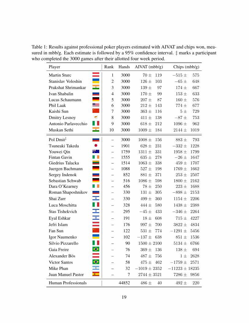
Table 1: Results against professional poker players estimated with AIVAT and chips won, mea-sured in mbb/g. Each estimate is followed by a 95% confidence interval. ‡ marks a participantwho completed the 3000 games after their allotted four week period.

Player Rank Hands AIVAT (mbb/g) Chips (mbb/g)

Martin Sturc 1 3000 70 ± 119 −515 ± 575

Stanislav Voloshin 2 3000 126 ± 103 −65 ± 648

Prakshat Shrimankar 3 3000 139 ± 97 174 ± 667

Ivan Shabalin 4 3000 170 ± 99 153 ± 633

Lucas Schaumann 5 3000 207 ± 87 160 ± 576

Phil Laak 6 3000 212 ± 143 774 ± 677

Kaishi Sun 7 3000 363 ± 116 5 ± 729

Dmitry Lesnoy 8 3000 411 ± 138 −87 ± 753

Antonio Parlavecchio 9 3000 618 ± 212 1096 ± 962

Muskan Sethi 10 3000 1009 ± 184 2144 ± 1019

Pol Dmit‡ – 3000 1008 ± 156 883 ± 793

Tsuneaki Takeda – 1901 628 ± 231 −332 ± 1228

Youwei Qin – 1759 1311 ± 331 1958 ± 1799Fintan Gavin – 1555 635 ± 278 −26 ± 1647

Giedrius Talacka – 1514 1063 ± 338 459 ± 1707

Juergen Bachmann – 1088 527 ± 198 1769 ± 1662

Sergey Indenok – 852 881 ± 371 253 ± 2507

Sebastian Schwab – 516 1086 ± 598 1800 ± 2162

Dara O’Kearney – 456 78 ± 250 223 ± 1688

Roman Shaposhnikov – 330 131 ± 305 −898 ± 2153

Shai Zurr – 330 499 ± 360 1154 ± 2206

Luca Moschitta – 328 444 ± 580 1438 ± 2388

Stas Tishekvich – 295 −45 ± 433 −346 ± 2264

Eyal Eshkar – 191 18 ± 608 715 ± 4227

Jefri Islam – 176 997 ± 700 3822 ± 4834

Fan Sun – 122 531 ± 774 −1291 ± 5456

Igor Naumenko – 102 −137 ± 638 851 ± 1536

Silvio Pizzarello – 90 1500 ± 2100 5134 ± 6766

Gaia Freire – 76 369 ± 136 138 ± 694

Alexander Bos – 74 487 ± 756 1 ± 2628

Victor Santos – 58 475 ± 462 −1759 ± 2571

Mike Phan – 32 −1019 ± 2352 −11223 ± 18235

Juan Manuel Pastor – 7 2744 ± 3521 7286 ± 9856

Human Professionals 44852 486 ± 40 492 ± 220

19

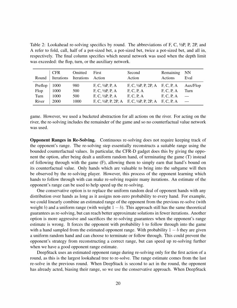
Table 2: Lookahead re-solving specifics by round. The abbreviations of F, C, ½P, P, 2P, andA refer to fold, call, half of a pot-sized bet, a pot-sized bet, twice a pot-sized bet, and all in,respectively. The final column specifies which neural network was used when the depth limitwas exceeded: the flop, turn, or the auxiliary network.

CFR Omitted First Second Remaining NNRound Iterations Iterations Action Action Actions Eval

Preflop 1000 980 F, C, ½P, P, A F, C, ½P, P, 2P, A F, C, P, A Aux/FlopFlop 1000 500 F, C, ½P, P, A F, C, P, A F, C, P, A TurnTurn 1000 500 F, C, ½P, P, A F, C, P, A F, C, P, A —River 2000 1000 F, C, ½P, P, 2P, A F, C, ½P, P, 2P, A F, C, P, A —

game. However, we used a bucketed abstraction for all actions on the river. For acting on theriver, the re-solving includes the remainder of the game and so no counterfactual value networkwas used.

Opponent Ranges in Re-Solving. Continuous re-solving does not require keeping track ofthe opponent’s range. The re-solving step essentially reconstructs a suitable range using thebounded counterfactual values. In particular, the CFR-D gadget does this by giving the oppo-nent the option, after being dealt a uniform random hand, of terminating the game (T) insteadof following through with the game (F), allowing them to simply earn that hand’s bound onits counterfactual value. Only hands which are valuable to bring into the subgame will thenbe observed by the re-solving player. However, this process of the opponent learning whichhands to follow through with can make re-solving require many iterations. An estimate of theopponent’s range can be used to help speed up the re-solving.

One conservative option is to replace the uniform random deal of opponent hands with anydistribution over hands as long as it assigns non-zero probability to every hand. For example,we could linearly combine an estimated range of the opponent from the previous re-solve (withweight b) and a uniform range (with weight 1− b). This approach still has the same theoreticalguarantees as re-solving, but can reach better approximate solutions in fewer iterations. Anotheroption is more aggressive and sacrifices the re-solving guarantees when the opponent’s rangeestimate is wrong. It forces the opponent with probability b to follow through into the gamewith a hand sampled from the estimated opponent range. With probability 1− b they are givena uniform random hand and can choose to terminate or follow through. This could prevent theopponent’s strategy from reconstructing a correct range, but can speed up re-solving furtherwhen we have a good opponent range estimate.

DeepStack uses an estimated opponent range during re-solving only for the first action of around, as this is the largest lookahead tree to re-solve. The range estimate comes from the lastre-solve in the previous round. When DeepStack is second to act in the round, the opponenthas already acted, biasing their range, so we use the conservative approach. When DeepStack

20

is first to act, though, the opponent could only have checked or called since our last re-solve.Thus, the lookahead has an estimated range following their action. So in this case, we use theaggressive approach. In both cases, we set b = 0.9.

Speed of Play. The re-solving computation and neural network evaluations are implementedon a GPU. This makes it possible to do fast batched calls to the counterfactual value networksfor multiple public subtrees at once, which is key to making DeepStack fast. It was implementedin Torch7 (43) and run on a single NVIDIA GeForce GTX 1080 graphics card.

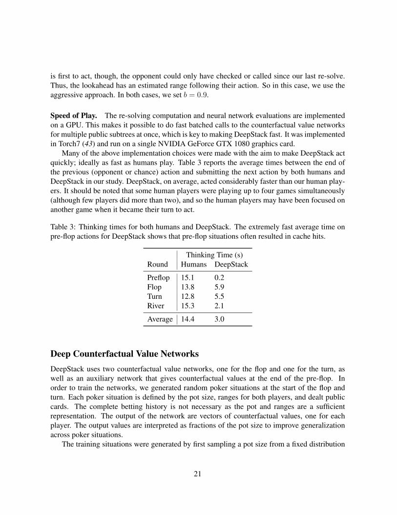
Many of the above implementation choices were made with the aim to make DeepStack actquickly; ideally as fast as humans play. Table 3 reports the average times between the end ofthe previous (opponent or chance) action and submitting the next action by both humans andDeepStack in our study. DeepStack, on average, acted considerably faster than our human play-ers. It should be noted that some human players were playing up to four games simultaneously(although few players did more than two), and so the human players may have been focused onanother game when it became their turn to act.

Table 3: Thinking times for both humans and DeepStack. The extremely fast average time onpre-flop actions for DeepStack shows that pre-flop situations often resulted in cache hits.

Thinking Time (s)Round Humans DeepStack

Preflop 15.1 0.2Flop 13.8 5.9Turn 12.8 5.5River 15.3 2.1

Average 14.4 3.0

Deep Counterfactual Value NetworksDeepStack uses two counterfactual value networks, one for the flop and one for the turn, aswell as an auxiliary network that gives counterfactual values at the end of the pre-flop. Inorder to train the networks, we generated random poker situations at the start of the flop andturn. Each poker situation is defined by the pot size, ranges for both players, and dealt publiccards. The complete betting history is not necessary as the pot and ranges are a sufficientrepresentation. The output of the network are vectors of counterfactual values, one for eachplayer. The output values are interpreted as fractions of the pot size to improve generalizationacross poker situations.

The training situations were generated by first sampling a pot size from a fixed distribution

21

which was designed to approximate observed pot sizes from older HUNL programs.7 Theplayer ranges for the training situations need to cover the space of possible ranges that CFRmight encounter during re-solving, not just ranges that are likely part of a solution. So wegenerated pseudo-random ranges that attempt to cover the space of possible ranges. We useda recursive procedure R(S, p), that assigns probabilities to the hands in the set S that sum toprobability p, according to the following procedure.

1. If |S| = 1, then Pr(s) = p.

2. Otherwise,

(a) Choose p1 uniformly at random from the interval (0, p), and let p2 = p− p1.(b) Let S1 ⊂ S and S2 = S \ S1 such that |S1| = b|S|/2c and all of the hands in S1

have a lower hand strength than hands in S2. Hand strength is the probability of ahand beating a uniformly selected random hand from the current public state.

(c) Use R(S1, p1) and R(S2, p2) to assign probabilities to hands in S = S1

⋃S2.

Generating a range involves invokingR(all hands, 1). To obtain the target counterfactual valuesfor the generated poker situations for the main networks, the situations were approximatelysolved using 1,000 iterations of CFR+ with only betting actions fold, call, a pot-sized bet, andall-in. For the turn network, ten million poker turn situations (from after the turn card is dealt)were generated and solved with 6,144 CPU cores of the Calcul Quebec MP2 research cluster,using over 175 core years of computation time. For the flop network, one million poker flopsituations (from after the flop cards are dealt) were generated and solved. These situations weresolved using DeepStack’s depth limited solver with the turn network used for the counterfactualvalues at public states immediately after the turn card. We used a cluster of 20 GPUS andone-half of a GPU year of computation time. For the auxiliary network, ten million situationswere generated and the target values were obtained by enumerating all 22,100 possible flopsand averaging the counterfactual values from the flop network’s output.

Neural Network Training. All networks were trained using the Adam stochastic gradientdescent procedure (32) using the average of the Huber losses over the counterfactual valueerrors. Training used a mini-batch size of 1000, and a learning rate 0.001, which was decreasedto 0.0001 after the first 200 epochs. Networks were trained for approximately 350 epochs overtwo days on a single GPU, and the epoch with the lowest validation loss was chosen.

Neural Network Range Representation. In order to improve generalization over input playerranges, we map the distribution of individual hands (combinations of public and private cards)

7The fixed distribution selects an interval from the set of intervals {[100, 100), [200, 400), [400, 2000),[2000, 6000), [6000, 19950]} with uniform probability, followed by uniformly selecting an integer from withinthe chosen interval.

22

into distributions of buckets. The buckets were generated using a clustering-based abstractiontechnique, which cluster strategically similar hands using k-means clustering with earth mover’sdistance over hand-strength-like features (31, 44). For both the turn and flop networks we used1,000 clusters and map the original ranges into distributions over these clusters as the first layerof the neural network (see Figure 3 of the main article). This bucketing step was not used on theauxiliary network as there are only 169 strategically distinct hands pre-flop, making it feasibleto input the distribution over distinct hands directly.

Neural Network Accuracies. The turn network achieved an average Huber loss of 0.016 ofthe pot size on the training set and 0.026 of the pot size on the validation set. The flop network,with a much smaller training set, achieved an average Huber loss of 0.008 of the pot size on thetraining set, but 0.034 of the pot size on the validation set. Finally, the auxiliary network hadaverage Huber losses of 0.000053 and 0.000055 on the training and validation set, respectively.Note that there are, in fact, multiple Nash equilibrium solutions to these poker situations, witheach giving rise to different counterfactual value vectors. So, these losses may overestimate thetrue loss as the network may accurately model a different equilibrium strategy.

Local Best Response of DeepStackLocal best-response (LBR) is a simple, yet powerful technique to produce a lower bound on astrategy’s exploitability (20). It explores a fixed set of options to find a “locally” good actionagainst the strategy. While it seems natural that more options would be better, this is not alwaystrue. More options may cause it to find a locally good action that misses out on a future op-portunity to exploit an even larger flaw in the opponent. In fact, LBR sometimes results in thelargest lower bounds when not considering any bets in the early rounds, so as to increase thesize of pot and thus the magnitude of a strategy’s future mistakes. As noted in the main text ofthe article, LBR was recently used to show that abstraction-based agents are significantly ex-ploitable. In all tested cases, the strategies were found to be even more exploitable than simplyfolding every game. As shown in Table 4, this is not true for DeepStack. Under all settingsof the LBR’s available actions, it fails to find any exploitable flaw in DeepStack. In fact, it islosing over 350 mbb/g to DeepStack. While this does not prove that DeepStack is flawless,it does suggest its flaws require a more sophisticated search procedure than what is needed toexploit abstraction-based programs.

Proof of Theorem 1The formal proof of Theorem 1, which establishes the soundness of DeepStack’s depth-limitedcontinuous re-solving, is conceptually easy to follow. It requires three parts. First, we estab-lish that the exploitability introduced in a re-solving step has two linear components; one due

23

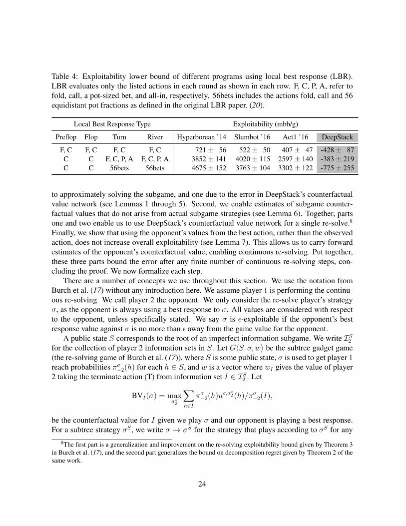
Table 4: Exploitability lower bound of different programs using local best response (LBR).LBR evaluates only the listed actions in each round as shown in each row. F, C, P, A, refer tofold, call, a pot-sized bet, and all-in, respectively. 56bets includes the actions fold, call and 56equidistant pot fractions as defined in the original LBR paper. (20).

Local Best Response Type Exploitability (mbb/g)

Preflop Flop Turn River Hyperborean ’14 Slumbot ’16 Act1 ’16 DeepStack

F, C F, C F, C F, C 721 ± 56 522 ± 50 407 ± 47 -428 ± 87C C F, C, P, A F, C, P, A 3852 ± 141 4020 ± 115 2597 ± 140 -383 ± 219C C 56bets 56bets 4675 ± 152 3763 ± 104 3302 ± 122 -775 ± 255

to approximately solving the subgame, and one due to the error in DeepStack’s counterfactualvalue network (see Lemmas 1 through 5). Second, we enable estimates of subgame counter-factual values that do not arise from actual subgame strategies (see Lemma 6). Together, partsone and two enable us to use DeepStack’s counterfactual value network for a single re-solve.8

Finally, we show that using the opponent’s values from the best action, rather than the observedaction, does not increase overall exploitability (see Lemma 7). This allows us to carry forwardestimates of the opponent’s counterfactual value, enabling continuous re-solving. Put together,these three parts bound the error after any finite number of continuous re-solving steps, con-cluding the proof. We now formalize each step.

There are a number of concepts we use throughout this section. We use the notation fromBurch et al. (17) without any introduction here. We assume player 1 is performing the continu-ous re-solving. We call player 2 the opponent. We only consider the re-solve player’s strategyσ, as the opponent is always using a best response to σ. All values are considered with respectto the opponent, unless specifically stated. We say σ is ε-exploitable if the opponent’s bestresponse value against σ is no more than ε away from the game value for the opponent.

A public state S corresponds to the root of an imperfect information subgame. We write IS2for the collection of player 2 information sets in S. Let G〈S, σ, w〉 be the subtree gadget game(the re-solving game of Burch et al. (17)), where S is some public state, σ is used to get player 1reach probabilities πσ−2(h) for each h ∈ S, and w is a vector where wI gives the value of player2 taking the terminate action (T) from information set I ∈ IS2 . Let

BVI(σ) = maxσ∗2

∑h∈I

πσ−2(h)uσ,σ∗2 (h)/πσ−2(I),

be the counterfactual value for I given we play σ and our opponent is playing a best response.For a subtree strategy σS , we write σ → σS for the strategy that plays according to σS for any

8The first part is a generalization and improvement on the re-solving exploitability bound given by Theorem 3in Burch et al. (17), and the second part generalizes the bound on decomposition regret given by Theorem 2 of thesame work.

24

state in the subtree and according to σ otherwise. For the gadget game G〈S, σ, w〉, the gadgetvalue of a subtree strategy σS is defined to be:

GVSw,σ(σS) =

∑I∈IS2

max(wI ,BVI(σ → σS)),

and the underestimation error is defined to be:

USw,σ = min

σSGVS

w,σ(σS)−∑I∈IS2

wI .

Lemma 1 The game value of a gadget game G〈S, σ, w〉 is∑I∈IS2

wI + USw,σ. (1)

Proof. Let σS2 be a gadget game strategy for player 2 which must choose from the F and Tactions at starting information set I . Let u be the utility function for the gadget game.

minσS1

maxσS2

u(σS1 , σS2 ) = min

σS1

maxσS2

∑I∈IS2

πσ−2(I)∑I′∈IS2

πσ−2(I′)

maxa∈{F,T}

uσS

(I, a)

= minσS1

maxσS2

∑I∈IS2

max(wI ,∑h∈I

πσ−2(h)uσS

(h))

A best response can maximize utility at each information set independently:

= minσS1

∑I∈IS2

max(wI ,maxσS2

∑h∈I

πσ−2(h)uσS

(h))

= minσS1

∑I∈IS2

max(wI ,BVI(σ → σS1 ))

= USw,σ +

∑I∈IS2

wI

Lemma 2 If our strategy σS is ε-exploitable in the gadget game G〈S, σ, w〉, then GVSw,σ(σS) ≤∑I∈IS2

wI + USw,σ + ε

Proof. This follows from Lemma 1 and the definitions of ε-Nash, USw,σ, and GVS

w,σ(σS).

25

Lemma 3 Given an εO-exploitable σ in the original game, if we replace a subgame with astrategy σS such that BVI(σ → σS) ≤ wI for all I ∈ IS2 , then the new combined strategy hasan exploitability no more than εO + EXPSw,σ where

EXPSw,σ =∑I∈IS2

max(BVI(σ), wI)−∑I∈IS2

BVI(σ)

Proof. We only care about the information sets where the opponent’s counterfactual valueincreases, and a worst case upper bound occurs when the opponent best response would reachevery such information set with probability 1, and never reach information sets where the valuedecreased.

Let Z[S] ⊆ Z be the set of terminal states reachable from some h ∈ S and let v2 be thegame value of the full game for player 2. Let σ2 be a best response to σ and let σS2 be the partof σ2 that plays in the subtree rooted at S. Then necessarily σS2 achieves counterfactual valueBVI(σ) at each I ∈ IS2 .

maxσ∗2

(u(σ → σS, σ∗2))

= maxσ∗2

[ ∑z∈Z[S]

πσ→σS

−2 (z)πσ∗22 (z)u(z) +

∑z∈Z\Z[S]

πσ→σS

−2 (z)πσ∗22 (z)u(z)

]

= maxσ∗2

[ ∑z∈Z[S]

πσ→σS

−2 (z)πσ∗22 (z)u(z)−

∑z∈Z[S]

πσ−2(z)πσ∗2→σS

22 (z)u(z)

+∑z∈Z[S]

πσ−2(z)πσ∗2→σS

22 (z)u(z) +

∑z∈Z\Z[S]

πσ−2(z)πσ∗22 (z)u(z)

]

≤ maxσ∗2

[ ∑z∈Z[S]

πσ→σS

−2 (z)πσ∗22 (z)u(z)−

∑z∈Z[S]

πσ−2(z)πσ∗2→σS

22 (z)u(z)

]

+ maxσ∗2

[ ∑z∈Z[S]

πσ−2(z)πσ∗2→σS

22 (z)u(z) +

∑z∈Z\Z[S]

πσ−2(z)πσ∗22 (z)u(z)

]

≤ maxσ∗2

[∑I∈IS2

∑h∈I

πσ−2(h)πσ∗22 (h)uσ

S ,σ∗2 (h)

−∑I∈IS2

∑h∈I

πσ−2(h)πσ∗22 (h)uσ,σ

S2 (h)

]+ max

σ∗2(u(σ, σ∗2))

26

By perfect recall π2(h) = π2(I) for each h ∈ I:

≤ maxσ∗2

[∑I∈IS2

πσ∗22 (I)

(∑h∈I

πσ−2(h)uσS ,σ∗2 (h)−

∑h∈I

πσ−2(h)uσ,σS2 (h)

)]+ v2 + εO

= maxσ∗2

[∑I∈IS2

πσ∗22 (I)πσ−2(I)

(BVI(σ → σS)− BVI(σ)

)]+ v2 + εO

≤[∑I∈IS2

max(BVI(σ → σS)− BVI(σ), 0)

]+ v2 + εO

≤[∑I∈IS2

max(wI − BVI(σ),BVI(σ)− BVI(σ))

]+ v2 + εO

=

[∑I∈IS2

max(BVI(σ), wI)−∑I∈IS2

BVI(σ)

]+ v2 + εO

Lemma 4 Given an εO-exploitable σ in the original game, if we replace the strategy in a sub-game with a strategy σS that is εS-exploitable in the gadget game G〈S, σ, w〉, then the newcombined strategy has an exploitability no more than εO + EXPSw,σ + US

w,σ + εS .

Proof. We use that max(a, b) = a+ b−min(a, b). From applying Lemma 3 withwI = BVI(σ → σS) and expanding EXPSBV(σ→σS),σ we get exploitability no more than

27

εO −∑

I∈IS2BVI(σ) plus∑

I∈IS2

max(BVI(σ → σS),BVI(σ))

≤∑I∈IS2

max(BVI(σ → σS),max(wI ,BVI(σ))

=∑I∈IS2

(BVI(σ → σS) + max(wI ,BVI(σ))

−min(BVI(σ → σS),max(wI ,BVI(σ))))

≤∑I∈IS2

(BVI(σ → σS) + max(wI ,BVI(σ))

−min(BVI(σ → σS), wI))

=∑I∈IS2

(max(wI ,BVI(σ)) + max(wI ,BVI(σ → σS))− wI

)=∑I∈IS2

max(wI ,BVI(σ)) +∑I∈IS2

max(wI ,BVI(σ → σS))−∑I∈IS2

wI

From Lemma 2 we get

≤∑I∈IS2

max(wI ,BVI(σ)) + USw,σ + εS

Adding εO −∑

I BVI(σ) we get the upper bound εO + EXPSw,σ + USw,σ + εS .

Lemma 5 Assume we are performing one step of re-solving on subtree S, with constraint val-ues w approximating opponent best-response values to the previous strategy σ, with an approx-imation error bound

∑I |wI − BVI(σ)| ≤ εE . Then we have EXPSw,σ + US

w,σ ≤ εE .

Proof. EXPSw,σ measures the amount that the wI exceed BVI(σ), while USw,σ bounds the amount

that the wI underestimate BVI(σ → σS) for any σS , including the original σ. Thus, together

28

they are bounded by |wI − BVI(σ)|:

EXPSw,σ + USw,σ =

∑I∈IS2

max(BVI(σ), wI)−∑I∈IS2

BVI(σ)

+ minσS

∑I∈IS2

max(wI ,BVI(σ → σS))−∑I∈IS2

wI

≤∑I∈IS2

max(BVI(σ), wI)−∑I∈IS2

BVI(σ)

+∑I∈IS2

max(wI ,BVI(σ))−∑I∈IS2

wI

=∑I∈IS2

[max(wI − BVI(σ), 0) + max(BVI(σ)− wI , 0)]

=∑I∈IS2

|wI − BVI(σ)| ≤ εE

Lemma 6 Assume we are solving a game G with T iterations of CFR-D where for both play-ers p, subtrees S, and times t, we use subtree values vI for all information sets I at the rootof S from some suboptimal black box estimator. If the estimation error is bounded, so thatminσ∗S∈NES

∑I∈IS2|vσ∗S(I)−vI | ≤ εE , then the trunk exploitability is bounded by kG/

√T+jGεE

for some game specific constant kG, jG ≥ 1 which depend on how the game is split into a trunkand subgames.

Proof. This follows from a modified version the proof of Theorem 2 of Burch et al. (17), whichuses a fixed error ε and argues by induction on information sets. Instead, we argue by inductionon entire public states.

For every public state s, let Ns be the number of subgames reachable from s, including anysubgame rooted at s. Let Succ(s) be the set of our public states which are reachable from swithout going through another of our public states on the way. Note that if s is in the trunk,then every s′ ∈ Succ(s) is in the trunk or is the root of a subgame. Let DTR(s) be the set ofour trunk public states reachable from s, including s if s is in the trunk. We argue that for anypublic state s where we act in the trunk or at the root of a subgame∑

I∈s

RT,+full(I) ≤

∑s′∈DTR(s)

∑I∈s′

RT,+(I) + TNsεE (2)

First note that if no subgame is reachable from s, then Ns = 0 and the statement follows fromLemma 7 of (14). For public states from which a subgame is reachable, we argue by inductionon |DTR(s)|.

29

For the base case, if |DTR(s)| = 0 then s is the root of a subgame S, and by assumption thereis a Nash Equilibrium subgame strategy σ∗S that has regret no more than εE . If we implicitlyplay σ∗S on each iteration of CFR-D, we thus accrue

∑I∈sR

T,+full(I) ≤ TεE .

For the inductive hypothesis, we assume that (2) holds for all s such that |DTR(s)| < k.Consider a public state s where |DTR(s)| = k. By Lemma 5 of (14) we have

∑I∈s

RT,+full(I) ≤

∑I∈s

RT (I) +∑

I′∈Succ(I)

RT,+full(I)

=∑I∈s

RT (I) +∑

s′∈Succ(s)

∑I′∈s′

RT,+full(I

′)

For each s′ ∈ Succ(s), D(s′) ⊂ D(s) and s 6∈ D(s′), so |D(s′)| < |D(s)| and we can applythe inductive hypothesis to show

∑I∈s

RT,+full(I) ≤

∑I∈s

RT (I) +∑

s′∈Succ(s)

∑s′′∈D(s′)

∑I∈s′′

RT,+(I) + TNs′εE

≤

∑s′∈D(s)

∑I∈s′

RT,+(I) + TεE∑

s′∈Succ(s)

Ns′

=∑

s′∈D(s)

∑I∈s′

RT,+(I) + TεENs

This completes the inductive argument. By using regret matching in the trunk, we ensureRT (I) ≤ ∆

√AT , proving the lemma for kG = ∆|IT R|

√A and jG = Nroot.

Lemma 7 Given our strategy σ, if the opponent is acting at the root of a public subtree Sfrom a set of actions A, with opponent best response values BVI·a(σ) after each action a ∈ A,then replacing our subtree strategy with any strategy that satisfies the opponent constraintswI = maxa∈A BVI·a(σ) does not increase our exploitability.

Proof. If the opponent is playing a best response, every counterfactual value wI before theaction must either satisfy wI = BVI(σ) = maxa∈A BVI·a(σ), or not reach state s with privateinformation I . If we replace our strategy in S with a strategy σ′S such that BVI·a(σ

′S) ≤ BVI(σ)

we preserve the property that BVI(σ′) = BVI(σ).

Theorem 2 Assume we have some initial opponent constraint values w from a solution gener-ated using at least T iterations of CFR-D, we use at least T iterations of CFR-D to solve each re-solving game, and we use a subtree value estimator such that minσ∗S∈NES

∑I∈IS2|vσ∗S(I)−vI | ≤

εE , then after d re-solving steps the exploitability of the resulting strategy is no more than(d+ 1)k/

√T + (2d+ 1)jεE for some constants k, j specific to both the game and how it is split

into subgames.

30

Proof. Continuous re-solving begins by solving from the root of the entire game, which welabel as subtree S0. We use CFR-D with the value estimator in place of subgame solving inorder to generate an initial strategy σ0 for playing in S0. By Lemma 6, the exploitability of σ0is no more than k0/

√T + j0εE .

For each step of continuous re-solving i = 1, ..., d, we are re-solving some subtree Si. Fromthe previous step of re-solving, we have approximate opponent best-response counterfactual val-ues BVI(σi−1) for each I ∈ ISi−1

2 , which by the estimator bound satisfy |∑

I∈ISi−12

BVI(σi−1)−

BVI(σi−1)| ≤ εE . Updating these values at each public state between Si−1 and Si as describedin the paper yields approximate values BVI(σi−1) for each I ∈ ISi

2 which by Lemma 7 canbe used as constraints wI,i in re-solving. Lemma 5 with these constraints gives us the boundEXPSi

wi,σi−1+ USi

wi,σi−1≤ εE . Thus by Lemma 4 and Lemma 6 we can say that the increase in

exploitability from σi−1 to σi is no more than εE + εSi≤ εE +ki/

√T + jiεE ≤ ki/

√T + 2jiεE .

Let k = maxi ki and j = maxi ji. Then after d re-solving steps, the exploitability is boundedby (d+ 1)k/

√T + (2d+ 1)jεE .

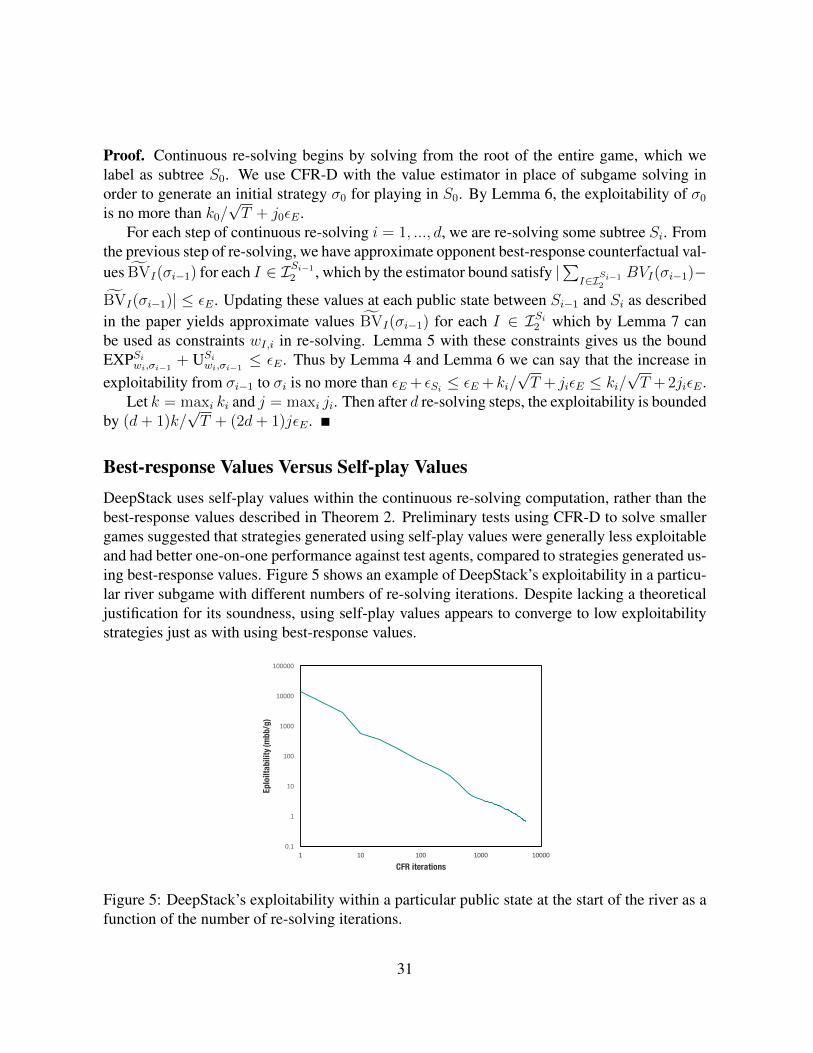
Best-response Values Versus Self-play ValuesDeepStack uses self-play values within the continuous re-solving computation, rather than thebest-response values described in Theorem 2. Preliminary tests using CFR-D to solve smallergames suggested that strategies generated using self-play values were generally less exploitableand had better one-on-one performance against test agents, compared to strategies generated us-ing best-response values. Figure 5 shows an example of DeepStack’s exploitability in a particu-lar river subgame with different numbers of re-solving iterations. Despite lacking a theoreticaljustification for its soundness, using self-play values appears to converge to low exploitabilitystrategies just as with using best-response values.

0.1

1

10

100

1000

10000

100000

1 10 100 1000 10000

Eplo

iltab

ility

(mbb

/g)

CFR iterations

Figure 5: DeepStack’s exploitability within a particular public state at the start of the river as afunction of the number of re-solving iterations.

31

One possible explanation for why self-play values work well with continuous re-solving isthat at every re-solving step, we give away a little more value to our best-response opponentbecause we are not solving the subtrees exactly. If we use the self-play values for the opponent,the opponent’s strategy is slightly worse than a best response, making the opponent valuessmaller and counteracting the inflationary effect of an inexact solution. While this optimismcould hurt us by setting unachievable goals for the next re-solving step (an increased US

w,σ

term), in poker-like games we find that the more positive expectation is generally correct (adecreased EXPSw,σ term.)

32